


![Deflation and augmentation techniques in Krylov …introduction to Krylov subspace methods and to [74] for a recent overview on Krylov subspace methods; see also [20, 21] for an advanced](https://static.fdocuments.in/doc/165x107/5edc1784ad6a402d66669cc6/deiation-and-augmentation-techniques-in-krylov-introduction-to-krylov-subspace.jpg)

Languages
Pages
Legal


The Extended Krylov Subspace for Matrix
Function Approximations:
Analysis and Applications
V. Simoncini
Dipartimento di Matematica, Universita di Bologna
Partially joint work with Leonid Knizhnerman, Moscow
1

The Problem
Given A ∈ Rn×n, v ∈ R
n and f sufficiently smooth function,
approximate
x = f(A)v
⋆ A large dimensions, ‖v‖ = 1
Applications:
• Numerical solution of evolution PDEs (e.g. exp(λ),√
λ−1, cos(λ), ...)
• Inverse Problems (exp(λ), cosh(λ), ...)
• Fluxes on manifolds
• Problems in Scientific Computing (e.g. QCD, sign(λ))
• (Analysis of) reduced Dynamical System Models (via Gramians)
2

The Problem
Given A ∈ Rn×n, v ∈ R
n and f sufficiently smooth function,
approximate
x = f(A)v
⋆ A large dimensions, ‖v‖ = 1
Projection-type methods
K approximation space, m = dim(K)
V ∈ Rn×m s.t. K = range(V )
x = f(A)v ≈ xm = V f(V ⊤AV )(V ⊤v)
Question: Which K ?
3

The Problem
Given A ∈ Rn×n, v ∈ R
n and f sufficiently smooth function,
approximate
x = f(A)v
⋆ A large dimensions, ‖v‖ = 1
Projection-type methods
K approximation space, m = dim(K)
V ∈ Rn×m s.t. K = range(V )
x = f(A)v ≈ xm = V f(V ⊤AV )(V ⊤v)
Question: Which K ?
4

Some explored alternatives for K
• Krylov subspace, K = Km(A, v)
• Shift-Invert Krylov subspace, K = Km((I + γA)−1, v) for some γ
• Rational Krylov subspace, for some ω1, ω2, . . .
K = span{v, (A − ω1I)−1v, (A − ω2I)−1v, . . .}
• Extended Krylov subspace, K = Km(A, v) + Km(A−1, A−1v)
• Restarted Krylov subspace
Note: In all cases, A nonsymmetric.
Theory mostly for field of values of A in C+
Field of values: W (A) = {x∗Ax, x ∈ Cn, ‖x‖ = 1}
5

Krylov subspace approximation
“Classical” approach:
K = Km(A, v) = span{v, Av, . . . , Am−1v}
For Hm = V ⊤m AVm, v = Vme1 and V ⊤
m Vm = Im:
xm = Vmf(Hm)e1
Polynomial approximation: xm = pm−1(A)v
(pm−1 interpolates f at eigenvalues of Hm)
⋆ Numerical and theoretical results since mid ’80s (Saad ’92)
6

Acceleration Procedures: Shift-Invert Krylov
Choose γ s.t. (I + γA) is invertible, and construct
K = Km((I + γA)−1, v), Moret-Novati ’04, van den Eshof-Hochbruck ’06
with Tm = V ⊤m (I + γA)−1Vm, v = Vme1 and V ⊤
m Vm = Im
xm = Vmf(1
γ(T−1
m − Im))e1
Rational approximation: xm = pm−1((I + γA)−1)v
Choice of γ: A spd, γ = 1√λminλmax
(Moret, 2009)
A nonsym, (Beckermann-Reichel tr2008)
7

Acceleration Procedures: Restarted Krylov
AV(1)m = V
(1)m H
(1)m + v
(1)m+1h
(1)m+1,me⊤m (V
(1)m )⊤V
(1)m = I
AV(2)m = V
(2)m H
(2)m + v
(2)m+1h
(2)m+1,me⊤m (V
(2)m )⊤V
(2)m = I
with V(2)m e1 = v
(1)m+1. Then
A[V (1)m , V (2)
m ] = [V (1)m , V (2)
m ]H2m + v(2)m+1h
(2)m+1,me⊤2m,
with
H2m =
H(1)m 0
e1h(1)m+1,me⊤m H
(2)m
.
Therefore (Eiermann-Ernst, ’06)
f(A)v ≈ x(1)m = V (1)
m f(H(1)m )
≈ x(2)m = V (1)
m f(H(1)m )e1 + V (2)
m f(H2m)e1|(2)x(2)
m = x(1)m + V (2)
m f(H2m)e1|(2)
8

Acceleration Procedures: Extended Krylov
For A nonsingular,
K = Km1(A, v) + Km2
(A−1, A−1v), Druskin-Knizhnerman 1998, A sym.
Note: K = A−m2Km1+m2(A, v)
Algorithm (augmentation-style)
- Fix m2 ≪ m1
- Run m2 steps of Inverted Lanczos
- Run m1 steps of Standard Lanczos + orth.
9

Extended Krylov: an effective implementation
m1 = m2 = m not fixed a priori
K = Km(A, v) + Km(A−1, A−1v)
= span{v, A−1v, Av, A−2v, A2v, . . .}
⋆ Block Arnoldi-type recurrence:
- U1 ← orth([v, A−1v])
- Uj+1 ← [AUj(:, 1), A−1Uj(:, 2)] + orth j = 1, 2, . . .
⋆ Recurrence to cheaply compute Tm = U⊤mAUm, Um = [U1, . . . , Um]
⋆ Compute xm = Umf(Tm)e1
Simoncini, 2007
10

Extended Krylov: Convergence theory I
f satisfying f(z) =
∫ 0
−∞
1
z − ζdµ(ζ), z ∈ C\] −∞, 0]
(with convenient measure dµ(ζ))
11

Extended Krylov: Convergence theory II
Nonsingular A, with 0 /∈ W (A).
Let Φ1, Φ2 be the conformal maps for W (A) and W (A)−1
There exists a > 0 s.t. |Φ1(−a)| = |Φ2(− 1a )| so that
‖f(A)v − Umf(Tm)e1 ‖ ≤ c
|Φ1(−a)|m
e.g. for A spd (Φ1, Φ2 known, a =√
λminλmax) :
‖x − xm‖ = O(exp(−2m 4
√λmin
λmax))
12
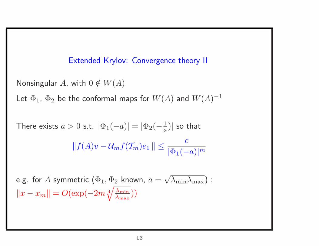
Extended Krylov: Convergence theory II
Nonsingular A, with 0 /∈ W (A)
Let Φ1, Φ2 be the conformal maps for W (A) and W (A)−1
There exists a > 0 s.t. |Φ1(−a)| = |Φ2(− 1a )| so that
‖f(A)v − Umf(Tm)e1 ‖ ≤ c
|Φ1(−a)|m
e.g. for A symmetric (Φ1, Φ2 known, a =√
λminλmax) :
‖x − xm‖ = O(exp(−2m 4
√λmin
λmax))
13

Convergence rate. A ∈ R400×400 normal. f(λ) = λ−1/2
0 5 10 15 20 25 30 35 4010
−12
10−10
10−8
10−6
10−4
10−2
100
102
dimension of approximation space
no
rm o
f e
rro
r
σ(A) on an elliptic curve in C+ with center on real axis
14

Rate. A ∈ R200×200 Jordan block, σ(A) = {4}. f(λ) = λ1/2
0 2 4 6 8 10 12 14 16 18 2010
−15
10−10
10−5
100
dimension of approximation space
norm of error
W (A) disk centered at 4 and unit radius
15

Large-scale numerical experiments
A from FD discretization of
L1(u) = −100ux1x1− ux2x2
+ 10x1ux1,
L2(u) = −100ux1x1− ux2x2
− ux3x3+ 10x1ux1
,
L3(u) = −e−x1x2ux1x1− ex1x2ux2x2
+1
x1 + x2ux1
,
L4(u) = −div(e3x1x2gradu) +1
x1 + x2ux1
on unit square/cube, Dirichlet hom. bc.
Inner system solves:
• Extended Krylov: systems with A solved with GMRES/AMG
• SI-Arnoldi: systems with I + γA solved with IDR(s)/ILU
16

An intermezzo
SI-Arnoldi requires getting the parameter γ:
10−8
10−7
10−6
10−5
10−4
10−3
10−2
10−1
100
101
55
65
155
205
255
305
355
405
450
value of parameter
nu
mb
er
of
ite
ratio
ns
SI−Arnoldi method
oper L1, n=10,000
oper L3, n=40,000
Number of SI-Arnoldi iterations as a function of the parameter for f(λ) = λ1/2
17

Comparisons: CPU Time in Matlab (space dim.)
f Oper. n SI-Arnoldi EKSM Std Krylov
λ1/2 L1 2500 0.9 (59) 0.6 (48) 7 (193)
10000 4.0 (66) 3.6 (68) *46 (300)
160000 642.9(246) 219.7(122) *458(300)
L2 27000 10.8 (55) 7.4 (40) 6.7(119)
125000 86.7 (60) 65.3 (52) 138.7(196)
L3 40000 26.3 (75) 21.1 (72) *87 (300)
160000 318.5(144) 173.3 (96) *442(300)
L4 40000 41.1(117) 25.4(106) *89 (300)
160000 580.2(442) 231.2(144) *461 (300)
18

Comparisons: CPU Time in Matlab (space dim.)
f Oper. n SI-Arnoldi EKSM Std Krylov
λ−1/3 L1 2500 0.6 (43) 0.4 (30) 2.2(131)
10000 2.6 (46) 1.8 (38) 26.2(252)
160000 79.3 (48) 99.7 (64) *460(300)
L2 27000 7.8 (41) 4.8 (26) 3.1 (82)
125000 64.8 (45) 38.9 (32) 67.5(138)
L3 40000 20.7 (61) 13.7 (48) *88 (300)
160000 116.5 (62) 105.2 (62) *460 (300)
L4 40000 35.8(104) 14.2 (66) *88 (300)
160000 208.1(104) 112.2 (84) *461 (300)
19

Stopping criterion
Unlike linear systems: no equation ⇒ no residual
Estimate of the error:
(first suggested for f(λ) = e−λ by van den Eshof-Hochbruck ’06)
‖x − xm‖‖xm‖ ≈ δm+j
1 − δm+j, δm+j =
‖xm+j − xm‖‖xm‖
Stopping criterion:
ifδm+j
1−δm+j≤ tol then stop
20

Computational costs awareness: inexact solves in EKSM
systems with A: GMRES with relaxed inner tolerance
ǫ(inner)m =
tolin
‖x − xm−1‖.
Final outer error (# outer its / # inner its)
tolin fixed inner tol relaxed inner tol
1e-10 6.97e-11 (24/901) 6.58e-11 (24/559)
1e-12 6.48e-11 (24/1052) 6.48e-11 (24/716)
L(u) = −uxx − uyy − uzz + 50(x + y)ux
f(λ) = λ−1/3 ǫ(outer) = 10−10
21

A special case: f(λ) = (λ − σ)−1. x = (A − σI)−1v ≡ fσ(A)v
All as before - and new perspective:
• Many shifts in a wide range (e.g., Structural dynamics, electromagn.)
(A − σjI)x = v, σj ∈ [α, β], large interval
j = 1, . . . , k, k = O(100)
• Few shifts (e.g., quadrature formulas)
z =
k∑
j=1
ωj(A − σjI)−1v
• Transfer function
h(σ) = c∗(A − iσI)−1b, σ ∈ [α, β]
22

Shifted systems (joint work with A. Frommer)
Extended Krylov subspace method:
x ≈ Umfσ(Tm)e1 = Um(Tm − σI)−1e1
standard Galerkin-type approximation for shifted systems
(cf. FOM, CG, ...)
Key fact: A single K for all shifted systems.
Shift invariance:
Km(A, v) = Km(A − σI, v)
Note: Solve systems with A to approximate (A − σI)−1v
23

Added feature: restarting made easy
AUm = UmTm + Um+1τττE⊤m
Proportionality of the residuals:
For xm(σ) = Um(Tm − σI)−1e1, the residual
rm(σ) := b − (A − σI)xm(σ), rm(σ) ∝ Um+1e2m+1 ∀σ
(typical of Galerkin-type procedures)
Restarting with a single approximation space:
K(2) = Km(A, v(2)) + Km(A−1, A−1v(2)), v(2) = Um+1e2m+1
x(2)m (σ) = x(1)
m (σ) + zm, zm ∈ K(2)
24

Added feature: restarting made easy
AUm = UmTm + Um+1τττE⊤m
Proportionality of the residuals:
For xm(σ) = Um(Tm − σI)−1e1, the residual
rm(σ) := b − (A − σI)xm(σ), rm(σ) ∝ Um+1e2m+1 ∀σ
(typical of Galerkin-type procedures)
Restarting with a single approximation space:
K(2) = Km(A, v(2)) + Km(A−1, A−1v(2)), v(2) = Um+1e2m+1
x(2)m (σ) = x(1)
m (σ) + zm, zm ∈ K(2)
25

An example from Structural Dynamics
(K⋆ − σ2M)x = b, ⇒ (K⋆M−1 − σ2I)x = b
K⋆ stiffness + hysteretic damping, M mass σ ∈ 2π[0.1, 60.1]
frequencies, n = 3627
number of restarts (subspace dimension)
restarted restarted
EKSM FOM
3 (20) - (20)
1 (34) 81(40)
21(80)
26

Transfer function approximation (cf. MOR)
h(σ) = c∗(A − iσI)−1b, σ ∈ [α, β]
Given space K and V s.t. K=range(V ),
h(σ) ≈ (V ∗c)∗(V ∗AV − σI)−1(V ∗b)
For K = Km(A, b) (standard Krylov):
hm(σ) = (V ∗mc)∗(Hm − σI)−1e1‖b‖
For K = Km(A, b) + Km(A−1, A−1b) (EKSM):
hm(σ) = (U∗mc)∗(Tm − σI)−1e1‖b‖
Alternative: Rational Krylov (Grimme-Gallivan-VanDooren etc. )
choosing the poles unresolved issue
27

An example: CD Player, |h(σ)| = |C∗:,i(A − iσI)−1B:,j |
10−1
100
101
102
103
104
105
106
10−8
10−6
10−4
10−2
100
102
104
106
108
CDplayer, m=20, (1,1)
truearnoldiextended
10−1
100
101
102
103
104
105
106
10−8
10−6
10−4
10−2
100
102
104
CDplayer, m=20, (1,2)
truearnoldiextended
10−1
100
101
102
103
104
105
106
10−7
10−6
10−5
10−4
10−3
10−2
10−1
100
101
102
CDplayer, m=20, (2,1)
truearnoldiextended
10−1
100
101
102
103
104
105
106
10−5
10−4
10−3
10−2
10−1
100
101
102
103
104
CDplayer, m=20, (2,2)
truearnoldiextended
28

An example: CD Player, |h(σ)| = |C∗:,i(A − iσI)−1B:,j |
10−1
100
101
102
103
104
105
106
10−8
10−6
10−4
10−2
100
102
104
106
108
CDplayer, m=20, (1,1)
truearnoldiextended
10−1
100
101
102
103
104
105
106
10−8
10−7
10−6
10−5
10−4
10−3
10−2
10−1
100
101
102
CDplayer, m=50, (1,2)
truearnoldiextended
10−1
100
101
102
103
104
105
106
10−7
10−6
10−5
10−4
10−3
10−2
10−1
100
101
102
CDplayer, m=20, (2,1)
truearnoldiextended
10−1
100
101
102
103
104
105
106
10−5
10−4
10−3
10−2
10−1
100
101
102
103
104
CDplayer, m=20, (2,2)
truearnoldiextended
29

Two-parameter linear systems (with F. Perotti - K. Meerbergen)
(A + βjB + αiI)x = v, x = x(αi, βj)
Commonly: #α = O(100), #β = O(10)
Problem: Solve all systems at a cost sublinear in #α,#β
Currently, Shifted restarted EKSM most efficient strategy:
For each βj , solve (A + βjB + αiI)x = v, ∀αi But: linear in β...
..The expensive way:
A
A
. . .
A
+
β1B
β2B
. . .
βkB
+ αiI
z = f
30

Two-parameter linear systems (with F. Perotti - K. Meerbergen)
(A + βjB + αiI)x = v, x = x(αi, βj)
Commonly: #α = O(100), #β = O(10)
Problem: Solve all systems at a cost sublinear in #α,#β
Currently, Shifted restarted EKSM most efficient strategy:
For each βj , solve (A + βjB + αiI)x = v, ∀αi But: linear in β...
..The expensive way:
A
A
. . .
A
+
β1B
β2B
. . .
βkB
+ αiI
z = f
31

Two-parameter linear systems (with F. Perotti - K. Meerbergen)
(A + βjB + αiI)x = v, x = x(αi, βj)
Commonly: #α = O(100), #β = O(10)
Problem: Solve all systems at a cost sublinear in #α,#β
Currently, Shifted restarted EKSM most efficient strategy:
For each βj , solve (A + βjB + αiI)x = v, ∀αi But: linear in β...
..The expensive way:
A
A
. . .
A
+
β1B
β2B
. . .
βkB
+ αiI
z = f
32

Conclusions
• Efficient generation of the Extended Krylov subspace
• Complete theory for EKSM for a large class of functions
• Performance:
- Competitive with respect to available methods
(when solving with A can be made cheap)
- Does not depend on parameters
- Projection-type method: wide applicability (work in progress)
[email protected], http://www.dm.unibo.it/~ simoncin
33
Top Related