


Languages
Pages
Legal


V CAN WE PREDICT THRESHOLDS WITHOUT CROSSING THEM?
Introduction
Previous chapters discussed the retrospective analysis of regime shifts. By
retrospective, I mean the backward-looking process of examining data, fitting models,
and drawing inferences about which models are appropriate descriptions of the
ecosystem’s behavior. The retrospective study of regime shifts is difficult, primarily
because regime shifts are relatively uncommon events. Nevertheless, regime shifts can
be discerned in ecosystem data, particularly when long-term observations are
supplemented with ecosystem experiments, comparisons of many ecosystems, or
studies that provide properly-scaled measurements of key process rates.
This chapter turns to the prediction of regime shifts. To predict, additional
assumptions are needed. For example, it is necessary to assume that we have the
appropriate model for the regime shifts, that we can predict the trends of extrinsic
drivers, and that parameter values are stable (or at least have predictable trends).
These conditions are difficult to meet, and the additional uncertainties contributed by the
added assumptions are hard to evaluate. Nevertheless, prediction of regime shifts is a
necessary step in hypothesis testing. As the study of regime shifts becomes a more
rigorous part of ecology, ecologists will want to test hypotheses about regime shifts by
predicting where and when they should occur. Thus research on prediction will help to
DRAFT: DO NOT CITE OR QUOTE 1

advance the basic science of regime shifts. The consideration of uncertainties and how
they should be propagated over time is one of the most important research frontiers in
this area (Clark et al. 2001, Carpenter 2002).
Today’s Actions Affect Tomorrow’s Predictions
Ecosystem managers may also need to predict regime shifts, and this need raises
further complications because actions based on predictions can change the future. In
management, the backward-looking understanding of regime shifts merges with the
forward-looking capability to manipulate ecosystems. By choosing actions based on
predictions of future ecosystem conditions, managers affect how the ecosystem
changes and thereby affect learning, by influencing the new observations available for
fitting predictive models.
The cycle of retrospective model fitting and forward-looking manipulations could
either improve or inhibit our ability to predict regime shifts. In Chapter IV the deliberate
manipulations of the experimental lakes revealed a regime shift in plankton dynamics at
a certain critical level of the planktivory index. The experimental manipulations were
designed to produce large changes in ecosystem dynamics. Such manipulations could
be used by managers to improve understanding of ecosystem dynamics, with benefits
for future management (Walters 1986, Kitchell 1992). What if instead the manipulations
had been designed to maintain the ecosystem in a particular condition, as is often the
goal of ecosystem management? In this case, the range of ecosystem responses
DRAFT: DO NOT CITE OR QUOTE 2

would have been limited, and the ability to discern the regime shift would have been
compromised. This reveals a fundamental conflict between the scientific goal of
understanding regime shifts and management to avoid them.
The conflict might be sidstepped if it is possible to anticipate regime shifts without
actually changing regimes. The purpose of this chapter is to explore that possibility,
using a specific example for a lake. In order to address the possibility of anticipating
regime shifts, we must consider both the retrospective analysis of available data and the
capacity to look forward. Whole-lake experiments in which the manipulations are
chosen for purely scientific reasons, like those described in Chapter IV, are relatively
rare because few lakes are available for experimentation and few funding agencies are
willing to support such large interdisciplinary experiments. Instead, most ecosystem
experiments are undertaken by managers, or by collaborative teams of scientists and
managers. In these situations, the benefits of better information about regime shifts are
balanced against the costs of potential damage to ecosystem resources. This more
complicated, but also more realistic, situation is considered in this chapter.
Before turning to the lake case study, I will discuss a global problem of predicting
abrupt climate change. In this situation, costs of crossing a threshold are high, data to
estimate the threshold are sparse, the system of interest is large, unique, and cannot be
replicated, and experimental manipulations to cross the threshold would be unwise even
if they were possible. This global problem is analogous in many ways to the problem of
a clear-water lake subject to eutrophication. In the lake case, costs of crossing the
DRAFT: DO NOT CITE OR QUOTE 3

threshold are high, data are often sparse, and experimental manipulations to find the
threshold may be risky. Because of these similarities, study of the lake management
problem may build intuition about the global climate problem. The main difference
between the global problem and the lake problem is that many lakes are available for
comparison and experimentation. Thus, experimentation using a few lakes to learn
about thresholds may have significant benefits for managing the whole population of
lakes on a landscape. That idea will be developed further in the next chapter. The
present chapter focuses on the case of a unique resource for which little prior
information is available. Most of the information about the threshold must be obtained
from the ecosystem being managed, but experimentation could cause the ecosystem
change that we wish to avoid. Is it possible to learn enough about the threshold to
avoid crossing it?
Continent at risk of ice age
Global pollution of the atmosphere has created a risk of abrupt climate change (Alley et
al. 2003). One pattern of concern involves catastrophic cooling of Europe. Europe’s
climate is moderated by the North Atlantic thermohaline circulation, a current system
that carries warm water from the tropics to northern latitudes. On a handful of
occasions in the past, the northward extent of warm surface water has been pushed
southward by melting of arctic ice (Taylor 1999). The cold fresh water from the melted
ice floats above the warmer but more saline (and therefore more dense) tropical water,
pushing the warm water below the surface of the North Atlantic ocean. This change in
DRAFT: DO NOT CITE OR QUOTE 4

circulation reduces the flux of heat from the ocean to the atmosphere. The heat of the
eastward-flowing winds to Europe is diminished. Europe cools rapidly and then
becomes covered by glaciers. These cooling events can be triggered in less than 10
years, and the subsequent glaciations of Europe last hundreds of years (Rahmstorf
1997, Taylor 1999). The events are analogous to eutrophication: underlying causes
build slowly and gradually, the regime shift is rapid, and the consequences last a long
time.
Currently, warming of Earth, caused at least in part by human burning of fossil
fuels, is causing rapid melting of polar ice. This melting could cut off the heat pump to
Europe by the same mechanisms that have occurred in the past (Broecker 1987).
The problem is analogous to lake eutrophication, but larger in scale. Nearly a
billion people live in Europe. Glaciation of Europe would be a massive disaster. All of
humanity uses the atmosphere to dilute pollutants, including the gases that contribute
to global warming and melting of polar ice. How can these competing interests be
resolved? What is the threshold rate of climate warming to change thermohaline
circulation? How much fossil fuel burning is acceptable if we wish to avoid glaciation of
Europe (Broecker 1987)? As in the lake case, the management problem is to estimate
the threshold and construct policies to stay away from it (Deutsch et al. 2002, Heal and
Kriström 2002).
Lake at risk of eutrophication
DRAFT: DO NOT CITE OR QUOTE 5

A lake in an agricultural region is valued for water supply, fishing, and recreational use.
It is also used to assimilate polluted runoff from farms. People are aware that the lake
could become eutrophic due to phosphorus pollution (Chapter II). If this occurs, the
drinking water supply, fish populations and recreational opportunities would all be
impaired or lost. On the other hand, agriculturalists need the lake to dispose of
phosphorus pollution from excess manure and mineral fertilizers. Thus there are
competing uses for the lake water (Fig. 32). One interest group would like to decrease
phosphorus inputs to reduce risk of eutrophication and maintain clean water for
drinking, fishing and recreation. A different interest group would like to increase
agricultural output, which will increase phosphorus pollution. How should these
competing goals be balanced?
In practice, the tradeoffs are settled through political competitions (Fig. 32) with
varying degrees of scientific input (Scheffer et al. 2000a). The scientific questions
center around the location of the threshold for eutrophication, and the economic costs
and benefits of the various uses of the lake such as drinking water, pollution dilution,
fishing and recreation. Frequently the costs of eutrophying the lake far outweigh the
benefits of using the lake to dilute pollution, because the value of clean water is high
and reversing eutrophication is expensive or impossible (Wilson and Carpenter 1999,
Carpenter et al. 1999b). Thus, in most cases a rational manager will seek to avoid
crossing the threshold to eutrophication.
DRAFT: DO NOT CITE OR QUOTE 6

If the location of the threshold is known, then one can estimate how much
pollution is acceptable if eutrophication is to be avoided (Carpenter et al. 1999b,
Ludwig et al. 2003, Peterson et al. 2003). One sure way to find the threshold is to cross
it, but this is undesirable because of the long time lags involved in recovery from
eutrophication. Thus the manager faces the dilemma of avoiding an unknown
threshold. One interest group will favor very low phosphorus pollution to be sure to
avoid the threshold, while the other interest group will favor higher rates of phosphorus
pollution. The political tension could be resolved by economic arguments if the location
of the threshold could be predicted. Can this be done without crossing the threshold?
The remainder of this chapter uses a simulation model of a managed lake to
explore the possibility of anticipating regime shifts before they occur. The next two
sections of the chapter describe the motivation for the model and the details of its
construction. Then, model results are presented and discussed. The general
conclusion is that it is very difficult to anticipate a regime shift without causing it to
happen, even with rather bold experiments. Indeed, the most informative experiments
cause a regime shift. On the other hand, a few simple, precautionary management rules
make it possible for management to prevent unwanted regime shifts. Such
precautionary management is not always compatible with experimentation on a
particular ecosystem.
Motivation for the Model
DRAFT: DO NOT CITE OR QUOTE 7

A regime shift in lake water clarity, as introduced in the previous section “Lake at risk of
eutrophication”, provides a case study for this chapter. Eutrophication is a significant
societal problem that is a focus of applied ecology and ecosystem management in many
parts of the world (Carpenter et al. 1998a). The regime shifts involved in eutrophication
are reasonably well understood (Chapters II and III). Slowly-changing variables, such
as soil or sediment phosphorus, could provide “leading indicators” of future
eutrophication (Bennett et al. 2001), so there is a possibility of anticipating regime shifts
before they occur. Many case studies of eutrophication have been published, and this
rich literature can be used to improve estimates of parameters necessary to predict the
regime shift (see Chapter III). Eutrophication causes substantial economic losses
(Wilson and Carpenter 1999) and reversal of eutrophication is expensive (Cooke et al.
1993), so economically rational management should strive to avoid the regime shift to
eutrophication (Carpenter et al. 1999b, Ludwig et al. 2003). Thus eutrophication is a
situation in which experimentation to measure thresholds may come into conflict with
the need to avoid crossing the thresholds.
To focus discussion, consider a lake subject to possible eutrophication through
the phosphorus cycling mechanisms discussed in Chapter II (Fig. 33). The manager
attempts to balance competing political and economic pressures while avoiding
eutrophication of the lake. Phosphorus concentration in the water is the central
concern. The phosphorus concentration in the water can change rapidly in response to
more gradual changes in phosphorus in the lake sediments and the soils of the
watershed. Management often focuses on controlling the mean rate of phosphorus
DRAFT: DO NOT CITE OR QUOTE 8

input to the lake, although there may also be uncontrollable stochastic fluctuations due
to weather. Management can act at several scales, ranging from in-lake manipulations
of phosphorus concentrations, to manipulations of inputs from tributary streams and
riparian land, to manipulations of soil phosphorus in the watershed. To simplify the
model for this chapter, I assumed that management actions would control the mean
annual input at the point of entry to the lake (Cooke et al. 1993). In practice, this
corresponds to point source controls such as sewage treatment, direct manipulations of
tributary streams (e.g. diversion of tributaries), or installation of riparian buffers to
intercept phosphorus inputs (Osborne and Kovacik 1993).
The model (described below) assumes that the economically optimal
management would avoid the regime shift to eutrophication. However, the model does
not compute an optimal policy. Instead, the management algorithms attempt to avoid
crossing the threshold, implicitly assuming that this is close to the optimal strategy. This
simplifying assumption is appropriate for the case of a lake with good water quality
subject to P inputs that may increase in the future (Carpenter et al. 1999b, Ludwig et al.
2003). In the case of a lake which is already eutrophic, or a lake in which sediment
phosphorus has accumulated to the point where eutrophication is inevitable, it may be
economically optimal to use the lake as a dump for pollutants and abandon any uses for
drinking water, fishing or recreation (Ludwig et al. 2003). Such a conclusion is highly
sensitive to the choice of economic discount factor used in the computation of the
optimal strategy (Ludwig et al. 2003). The situation in which it is economically optimal
to pollute the lake is not considered in this chapter.
DRAFT: DO NOT CITE OR QUOTE 9

Management, in the model, operates by simple rules that seek to avoid the
threshold. In some cases, the rules also seek to improve parameter estimates. These
simple rules are a plausible representation of typical strategies of managers in the field.
Most lake managers are aware of the possibility of a regime shift, and act to avoid
eutrophication. Most managers do not perform an economic cost-benefit analysis at
each time step. They know that economic analyses generally show that the clear-water
state is far more valuable than the eutrophic one (Carpenter et al. 1999b, Wilson and
Carpenter 1999), and they assume that clear water is economically preferable.
However, managers are continually pressured by some interest groups to increase
phosphorus inputs to the lake, and to justify their targets for phosphorus inputs
(Scheffer et al. 2000a). This creates a tension between increasing the phosphorus
input while avoiding the threshold of eutrophication. This tension is addressed in
different ways by the management strategies described below.
I will assume that the manager invests in observations of the concentration of
phosphorus in the lake water and the amount of phosphorus in the sediment (Fig. 33).
Because I have assumed that phosphorus input control occurs immediately upstream of
the lake, this chapter will not address phosphorus content of soils. Although soil
phosphorus content is perhaps the best control variable for managing eutrophication
(Bennett et al. 2001), my points about anticipation of regime shifts can be made without
including the complications of soil phosphorus in the model. I assume that the manager
fits a predictive model for the ecosystem to available data at each time step. Based on
DRAFT: DO NOT CITE OR QUOTE 10

this predictive model and specified goals for phosphorus in the lake, the manager
chooses an input target for the next time step. The precision of the model predictions
depends on the data that are available to fit the model. This creates a tension between
experimentation to improve the data and the risk that the experiments might create a
regime shift. How much can the manager learn about the threshold without crossing it?
And how will different management strategies affect learning and risk?
DRAFT: DO NOT CITE OR QUOTE 11

Model
For the purposes of this chapter, I built a simple model of a lake ecosystem subject to
eutrophication, interacting with a management system that attempts to avoid
eutrophication (Fig. 34). The manager observes the lake, and fits a model which is
used to predict the future condition of the lake. Given these predictions, a phosphorus
input target is chosen using a specified management strategy.
In building this model, a number of specific assumptions were necessary and
these are detailed below. The rationale for these assumptions follows from the
overarching goal of the exercise, which is to explore the possibility of anticipating
thresholds before they occur. We shall see that this proves very difficult. The major
assumptions of the model were chosen to make it easier to anticipate thresholds. In
reality, it will be more difficult to anticipate thresholds than it is in this model. Because it
is difficult to anticipate regime shifts in the model, and the model is biased in favor of
anticipating regime shifts, the results strongly suggest that regime shifts will be difficult
to anticipate in actual management situations.
The model (Fig. 34) combines an ecosystem model of phosphorus dynamics in
lake water and sediment, a statistical model for dynamic learning of unknown
parameters, and a policy for choosing phosphorus inputs (Fig. 34). Each year, a mean
input target is set for the lake based on current information. The actual phosphorus
input is subject to random shocks around the mean, due to random effects such as
DRAFT: DO NOT CITE OR QUOTE 12

weather. Given the actual input, levels of phosphorus in sediments and water are
calculated using the ecosystem model. We assume that the managers of the
ecosystem do not know the parameters for the dynamics of the ecosystem, and must
estimate them from data. Based on observed time series, parameters for an estimated
model for ecosystem dynamics can be calculated at each time step. Managers choose
the mean input target for the next year using their estimated model and a management
strategy.
The remainder of this chapter presents details of the model in four subsections.
The first three subsections present the ecosystem model, the statistical model for
observing the ecosystem and predicting its future condition, and the management
strategies to be compared. Because the model is stochastic, it is difficult to draw
conclusions about the management strategies from a single run of the model.
Therefore Monte Carlo simulations were conducted to characterize the distribution of
outcomes under each management strategy. The methods for the Monte Carlo
simulations are described in the fourth subsection.
Ecosystem Model
Dynamics of phosphorus in sediment and water followed the model used by Dent et al.
(2002) and Ludwig et al. (2003). Dynamic equations are
Mt+1 = Mt + s Pt – b Mt – r Mt [ Ptq / (mq + Pt
q) ] (8)
DRAFT: DO NOT CITE OR QUOTE 13

Pt+1 = Pt + L exp[zt – (σ2 / 2)] - (s + h) Pt + r Mt [ Ptq / (mq + Pt
q) ] (9)
M is mass of phosphorus in the lake sediments and P is mass of phosphorus in the lake
water (both subscripted by time and with units g m-2). L is mean P input flux (g m-2 y-1)
and zt is the annual disturbance of P input which is assumed to be normally distributed
with mean zero and variance σ2. The quantity σ2 / 2 is subtracted from zt to cause the
mean value of exp[zt – (σ2 / 2)] to be unity (Hilborn and Mangel 1997). Thus realized P
input each year is a lognormally distributed random variate with mean L. Parameter
definitions and values used for simulations are presented in Table 3.
I assume that P mass in the water is directly proportional to phytoplankton
biomass. This assumption is corroborated by many limnological studies. In lakes
where primary production is controlled by phosphorus, most of the phosphorus is
contained in plant biomass during the growing season (Kalff 2002).
This model has three equilibria: a stable clear-water regime (low P or
oligotrophic), a stable turbid regime (high P or eutrophic), and an unstable point at
intermediate P (Chapter II; also see Dent et al. 2002, Ludwig et al. 2003). If the lake is
in the clear-water regime, a large random input event can shift P level above the
unstable point into the turbid regime. Once the lake has entered the turbid regime, the
excess P accumulates in sediments and is repeatedly recycled to the overlying water.
DRAFT: DO NOT CITE OR QUOTE 14

Therefore, several years of low P input are required to shift the lake from the turbid
regime to the clear-water regime.
The critical P input rate declines with the mass of phosphorus in the sediment
(Fig. 35). The critical P input rate is the threshold for transition from the clear-water
regime to the turbid regime, which was discussed in Chapter II. P input events larger
than the critical P input rate will shift the lake from the clear-water regime to the turbid
regime. The threshold for the opposite transition – from the turbid regime to the clear-
water regime – occurs at much lower P input rates (Carpenter et al. 1999b). This
chapter concerns the transition from clear water to the turbid regime.
Parameter values were chosen to place the ecosystem in the clear-water regime,
but near the threshold for transition to the eutrophic regime (Table 3). This is the region
where information about the critical P input rate is most useful for maintaining clear
water (Carpenter 2001). The critical P input rate can be calculated from the parameters
of the ecosystem model. The precision of the estimate of the critical P input rate is
directly related to the information available to estimate the parameters.
Statistical Estimation
The goal of the statistical component of the model is to simulate a plausible scheme for
monitoring the ecosystem, updating parameter estimates for an ecosystem model, and
drawing inferences to guide management decisions. These goals could be met in many
DRAFT: DO NOT CITE OR QUOTE 15

ways. The approach described below is arbitrary, but plausible. Where necessary
simplifications were likely to introduce bias, the model is biased in favor of correctly
predicting the threshold. Thus the analysis is likely to be overly optimistic about
prospects for predicting the threshold. As noted above, the chapter concludes that it is
difficult to predict the threshold. Because the analysis was designed to be overly
optimistic, this pessimistic conclusion is likely to be robust.
I assumed that the manager knows the correct structural model (Equations 8 and
9) and must estimate the parameters from time-series data. In an actual application,
the correct structural model would be unknown, and model selection would add
uncertainty to the analysis (Peterson et al. 2003). In the real world of lake
management, then, predicting the threshold is even more difficult than my model
suggests.
I assume that the manager measures P mass in the lake water and P input each
year, a common practice in lake management programs. Observation error is assumed
to be negligible for P mass in the water, as can occur in monitoring programs with
extensive replication. Errors in P input measurements, however, are likely to be
nontrivial because of the high temporal variability of input events. Log(P input) is
assumed to be observed with normally-distributed errors (mean zero, standard deviation
0.07). M is rarely measured in lake management programs, so there is little precedent
for designing a statistical approach. I assumed that managers invested in a spatially-
intensive sampling program which estimated M with a coefficient of variation of 12.5%.
DRAFT: DO NOT CITE OR QUOTE 16

This is perhaps overly optimistic, but if so it biases the model in favor of successful
predictions. In preliminary simulations, changes in M over time were too small to be
useful for updating parameter estimates. Therefore, dynamics of M were ignored in the
estimation.
Parameter estimates were updated each year using Bayesian nonlinear dynamic
regression (Appendix). This method is appropriate because slow changes in M could
be captured as slow drift in the parameters. The Bayesian scheme can be computed
rapidly (an advantage for Monte Carlo analyses, see below) and makes it easy to
experiment with the precision of prior information available to the manager. Estimates
of mean parameter values from Bayesian nonlinear dynamic regression had only trivial
differences from maximum likelihood estimates using 30 years of simulated data.
However, the Bayesian nonlinear dynamic regression does not adequately represent
the full posterior distribution of the parameters (because of the Taylor approximation
employed in the updating, see Appendix). This would be important if the lake was to be
managed by optimal control methods which require integrations over such a posterior
distribution (Carpenter et al. 1999b, Ludwig et al. 2003, Chapter VI). The model
presented here does not include optimal control, so a full analysis of the posterior
distribution is not essential.
Bayesian nonlinear dynamic regression was implemented with an observation
vector of two elements, log(P input) and P. Parameters to be estimated are log(λ)
(corresponds to log(L) ), θ (corresponds to 1 – (s+h) ), ρ (corresponds to r Mt), and η
DRAFT: DO NOT CITE OR QUOTE 17

(corresponds to m). For simulations presented here, the prior distributions of the
parameters were assumed to be Student-t distributions with one degree of freedom and
mean values as in Table 3. Scale factors were calculated assuming coefficients of
variation of 10% for log(λ), 20% for θ and ρ, and 30% for η. This prior distribution
represents an informative parameter distribution, as might be estimated from a multi-
lake data set. Initial parameter estimates were drawn randomly from the prior
distribution. Note that q is assumed to be known precisely. This is unrealistic, and
biases the analysis toward successful prediction of the threshold.
Management Strategies
Five management strategies were compared (Table 4). In the Trial-and-Error strategy,
the manager attempts to find a P load rate that balances the need to avoid regime shift
with the pressure from constituents who wish to increase P inputs to the lake. The
water quality is deemed acceptable if the P level in the lake remains below 1. The
manager attempts to find the P loading rate that will maintain this P level by making
small adjustments to the P load depending on the current level of P in the lake.
In the passive strategy, the manager simply holds the P load rate at a fixed target
value that is deemed acceptable. In practice, this would be a level that balanced the
interests of constituents who wish to increase P inputs to the lake with those who wish
to maintain the lake in the clear-water state.
DRAFT: DO NOT CITE OR QUOTE 18

In the passive precautionary strategy, the manager reduces the P load to the
lake if key indicator variables are too high. One indicator variable is last year’s P load to
the lake. If it exceeds the expected P load plus a standard deviation, the next year’s P
load is scaled back to compensate for the impact of the exceptionally high load in the
preceding year. A second indicator variable is the recycling rate estimated from the
model, which is directly related to the possibility of regime shift. If the estimated
recycling rate can account for more than 1% of the P in the lake water, then load is
scaled back to compensate for the impact of recycling.
In the passive precautionary strategy, the decisions of the manager depend on
the predictions of P loading and the estimates of recycling. Both of these indicators will
be more accurate if the estimates of model parameters are more precise. The precision
of the parameter estimates could potentially be improved by experimentation.
In the experimental strategy, P input rates are selected from an experimental
design. Using exploratory simulations, I investigated alternative experimental designs.
The one used here is relatively simple, and yields data that can provide relatively
precise parameter estimates in 20 or 30 years. It is not feasible to obtain accurate
parameter estimates with less than about 20 years of data.
In the actively adaptive precautionary strategy, the precautionary rules are
combined with the experimental design. If the key indicators (P load rate and recycling
rate) are too high, the precautionary rule is applied and P load is decreased to 25% of
DRAFT: DO NOT CITE OR QUOTE 19
the nominal value. If the key indicators are acceptably low, then P load is selected
randomly from the experimental design. Thus experiments are performed only when
conditions are thought to be safe.
Monte Carlo Analyses
This model includes stochastic shocks at each time step. To understand the behavior
of the model, it is useful to study the frequency distribution of a large number of
simulations. These distributions were obtained by running the model 1000 times from
the same initial conditions for a given management strategy. The outcome represents
the frequency distribution obtained from randomly-chosen sequences of stochastic
shocks under a particular management strategy.
Results
Management Strategies and Regime Shifts
Choice of management strategy had strong effects on the probability of regime shift to
the eutrophic state (Table 5). Under the trial-and-error and experimental strategies, the
probability of eutrophication was high, roughly 70%. Under the actively adaptive
precautionary strategy, the probability of eutrophication was somewhat reduced. Under
the passive strategy, the probability of eutrophication was lower still. The passive
precautionary strategy had the lowest probability of eutrophication, about 5%.
DRAFT: DO NOT CITE OR QUOTE 20

Management Strategies, Regime Shifts and Learning
Parameter estimates were improved by experimentation. Time series presented in
Figs. 36 and 37 are from a model run in which management was experimental, but no
regime shift occurred. P and L exhibit variability due to the experimental treatments
(Fig. 36A,B). One-step-ahead predictions of P and log(L) were reasonably accurate.
Although recycling was high in a few years, it was not sufficient to trigger a regime shift
(Fig. 37C). The time series of P load treatments is presented in Fig. 37A. Experimental
treatments have some effect on parameter estimates (Fig. 37B-D). The most notable
improvement is seen in η (estimator of m), where the estimate draws closer to the
nominal value and the standard deviation declines. The mean value of ρ (estimator of r
M) changes slightly in the direction of the nominal value, but the standard deviation
grows. Changes in the estimate of θ (estimator of 1 – (s+h) ) are negligible.
Parameter estimates improved sharply if a regime shift occurred (Figs. 38 and
39). The regime shift was triggered by a larger-than-expected input event in year 10,
coincident with a jump in recycling the same year. The estimates of recycling
parameters ρ (estimator of r M) and η (estimator of m) improved immediately (Fig. 39).
Mean parameter estimates moved closer to the nominal values, and standard
deviations shrank. The estimate of θ (estimator of 1 – (s+h) ) deteriorated after the
regime shift, moving slightly away from the nominal value with slightly larger standard
DRAFT: DO NOT CITE OR QUOTE 21
deviation. After the regime shift, the estimate of recycling (which depends only on ρ
and η) and the estimate of the threshold for regime shift are markedly more accurate.
The improvement of parameter estimates after a regime shift makes sense. After
the regime shift has occurred, we have some basis for evaluating where the regime shift
occurs. We also have measurements across a wide range of P levels, which leads to
more precise parameter estimates.
Recycling rate typically increased one or two time steps prior to the regime shift
(Fig. 38). Any indicator that depends on the second derivative of observed P in the
water will jump prior to a regime shift. Sometimes the signal is helpful in preventing a
regime shift (e.g. Fig. 36 at Time steps 6 and 15). In other cases, the reduction in P
inputs following the signal is insufficient to prevent a regime shift (e.g. Fig. 38).
Active adaptive management consistently improved the estimates of recycling
rate (Fig. 40A). Bias is the difference between the recycling rate estimated by the
manager and the true recycling rate. Under active adaptive management, bias clusters
more tightly around zero than under passive management. However, most of the power
of active adaptive management derives from the regime shifts that it creates (Fig. 40B).
When we compare simulations in which a regime shift occurred, the bias of recycling
rate is about the same for the passive strategy and the active adaptive strategy.
Simulations in which no regime shift occurred have much higher frequency of large bias
(whether positive or negative) than simulations in which a regime shift occurred. There
DRAFT: DO NOT CITE OR QUOTE 22
are some minor differences between the passive strategy and the active adaptive
strategy, but the least-biased estimates of recycling occur in simulations with regime
shifts.
Discussion
The management strategies were chosen to explore two tensions. The tension
between those who wish to increase inputs to the lake and those who wish to avoid the
regime shift is illustrated by the trial-and-error strategy. This strategy has a high
probability of shifting the lake to the eutrophic state. Trial-and-error is a poor way to
manage a system subject to regime shifts. This leads to the second tension, that
between the need for precaution and the desire to learn about the regime shift.
Knowledge of the regime shift should assist the manager in setting limits or targets on P
loading, but gaining this knowledge runs the risk of regime shift. The experimental
management strategy was as risky as trial-and-error. The actively adaptive strategy
was better, but still had a high risk of regime shift.
The model used in this chapter was deliberately biased in favor of successfully
measuring model parameters and the threshold, while avoiding crossing the threshold.
The model assumes that the correct dynamic equations for the ecosystem are known,
prior parameter distributions are informative, regular monitoring programs are in place,
and the manager can rapidly (within one time step) change P inputs to desired levels.
All of these assumptions are optimistic. The assumption of rapid controllability of P
DRAFT: DO NOT CITE OR QUOTE 23

inputs is not realistic. Even under these favorable conditions, it was not possible to
improve estimates of parameters without crossing the threshold. In a more realistic
situation, prediction of thresholds will be far more difficult.
Experimental or actively adaptive management improved parameter estimates,
but the improvement is due almost entirely to the regime shifts caused by the
manipulations. For the ecosystem model analyzed here, it is very difficult to improve
parameter estimates without causing a regime shift. Similar conclusions were reached
by Walters (1986) and are evident in the statement that “To find out what happens to a
system when you interfere with it, you have to interfere with it (not just passively
observe it).” (Box 1966).
Implications for lake management
Certain indicators can help to prevent regime shifts if rapid, extreme management
responses are possible. Indicators related to the second derivative of P in the water,
such as recycling rate, were useful leading indicators in this model. However, the lead
time of the advance warning is short, only one time step. By the time the indicator
changes, the slow variable of sediment phosphorus is taking effect and eutrophication
may not be avoidable. Also, an unlucky stochastic shock could tip the system toward
eutrophication even if appropriate management action is taken. By the time the
indicator changes, there is a chance, but not a certainty, that swift, massive reductions
in P input can prevent the regime shift. In the case of real lakes subject to
DRAFT: DO NOT CITE OR QUOTE 24
eutrophication, such swift and massive responses are not likely because of the
difficulties of controlling nonpoint P inputs (Carpenter et al. 1998a). If it were actually
implemented for lakes at risk of eutrophication, the management system described in
this chapter would have a high failure rate.
Precautionary management can prevent most regime shifts in this model. The
simulations employ simple rules that were effective for reducing the probability of a
regime shift. These rules, however, assume that draconian steps can be taken within a
year to reduce P inputs. In real management situations, such rigorous year-by-year
management of P inputs is not possible. Instead, policies to avoid regime shifts should
maintain low levels of P in watershed soils and lake sediments, and thereby create a
large domain of attraction for the clear-water regime (Carpenter et al. 1999b, Bennett et
al. 2001, Dent et al. 2002). Such policies would also reduce P loads. For
eutrophication, precautionary policies maintain the resilience of the clear-water regime:
minimize point source inputs of P, reduce levels of P in watershed soils, and maintain
riparian buffers (Carpenter 1998).
Implications for actively adaptive management
In these simulations, I have not attempted to find the experimental design that is
optimal, in the sense of maximizing the probability of detecting the threshold. Such
experimental designs are discussed by Walters (1986) and Wieland (2000). Optimal
experimental designs may lead to better parameter estimates than the designs
DRAFT: DO NOT CITE OR QUOTE 25

employed here. However, such designs are unlikely to alter the conclusion that the best
way to determine the threshold for a regime shift is to cause a regime shift.
If the only way to learn about a regime shift is to observe one, then experimental
management as practiced in this chapter is unsafe for any specific ecosystem.
However, there are other approaches to actively adaptive management. Even for
singular ecosystems it may be possible to assess the processes that maintain the
stability of the regime that the manager prefers. This assessment could involve safe
experiments that do not create regime shifts but do explore aspects of the system that
may improve management. For example, in a model of eutrophication that included
agricultural practices and soil P, as well as sediment and water P, the threshold for
regime shift was a moving target (Carpenter et al. 1999a). In simulations with this
model, frequent experimentation with agricultural practices provided information about
the sensitivity of the lake which could be used to adjust the risk of regime shift. In this
more realistically complex model, active adaptive management proved useful for
assessing options that could avoid an undesirable regime shift. Active adaptive
management has other important advantages that are not addressed in this chapter.
For example, it fosters flexible and open institutions and multi-level decision systems
that allow for learning and tend to increase the likelihood of successful management
(Gunderson et al. 1995, Ostrom et al. 1999, Berkes et al. 2002, Folke et al. 2002a, b).
While certain types of experiments are dangerous for individual ecosystems, the
situation may be quite different for a set of modular ecosystems such as landscapes
DRAFT: DO NOT CITE OR QUOTE 26

with a large number of lakes (Levin 1999). Multi-lake comparative data sets have
proven extremely useful for understanding the P cycle and eutrophication in lakes
(Schindler et al. 1978, Reckhow and Chapra 1983, Rigler and Peters 1995). In the
context of this model, the multi-lake data would provide prior distributions for the
parameters. Simulations presented in this chapter suggest that informative prior
distributions are extremely useful for estimating recycling rates or the threshold for
regime shift. Prior distributions of parameters changed little over time in these
simulations unless a regime shift occurred.
The value of comparable data sets from multiple ecosystems adds another
dimension to adaptive ecosystem management. In cases where a large number of
similar ecosystems are available, it may be possible to experiment on a few ecosystems
to obtain data that are informative about thresholds in other ecosystems. While
comparative analysis is one of the pillars of ecosystem ecology (Cole et al. 1991),
comparative ecosystem studies have rarely been used to estimate thresholds and this
appears to be an important research frontier. The method of Bayesian inverse
modeling (Appendix) is a natural method for combining comparative ecosystem data
with local time-series observations to estimate parameters for thresholds or other
ecosystem properties.
Summary
DRAFT: DO NOT CITE OR QUOTE 27

This chapter considers the problem of managing a single ecosystem subject to regime
shift, given limited prior information about the threshold for change to an undesirable
regime. Is it possible to learn the location of the threshold without crossing it? What are
the tradeoffs between precaution to avoid the regime shift and experimentation to learn
the location of the threshold? This is a generic problem in ecosystem management. In
this chapter it was explored using the example of a clear-water lake subject to
eutrophication.
Trial and error is a risky strategy for managing systems subject to regime shift. It
combines high probability of regime shift with slow rates of learning about the
ecosystem.
There is a conflict between precautionary management and experimental
management. Precautionary management can prevent regime shifts, but provides little
information about the location of thresholds. Experimental management can reveal the
location of thresholds, at the cost of crossing them. Experiments that manipulate P
input prove risky. Other types of experiments, such as those to measure the rate of P
recycling or other key parameters, may provide useful information with less risk. The
appropriate design for such studies will differ among ecosystems and management
circumstances.
When managing a single ecosystem, the parameters for predicting a regime shift
can be learned, but this learning seems to require observing a regime shift. If the new
DRAFT: DO NOT CITE OR QUOTE 28

regime is highly undesirable, then precautionary management to minimize risk of regime
shift is preferable to experimentation. In the simulations presented in this chapter,
precaution and learning are incompatible. One can either create a regime shift and
thereby learn the location of the threshold, or attempt to avoid the threshold and thereby
leave its location shrouded in uncertainty. In a world with growing demand for
ecosystem resources, it will be difficult to justify precautionary policies without better
knowledge of thresholds. Such knowledge comes hard. The precautionary manager
will have difficulty building information about the threshold necessary to rationalize the
precautionary policies. Thus there is great risk that precautionary policies will give way
to trial-and-error.
The situation is different when a large number of similar ecosystems are to be
managed, as is the case for most lakes. The example of Lake Mendota (Chapter III)
showed that information from other lakes was extremely helpful in predicting recycling, a
key parameter for predicting regime shifts. Information from other lakes can narrow the
probability distribution of parameter estimates, and would in fact dominate the analysis
unless a regime shift occurred. Thus information from multiple lakes will improve the
performance of management strategies that depend on accurate predictions of
ecosystem thresholds.
For modular ecosystems with many separate replicates on the landscape, active
adaptive management may offer significant advantages. Information useful for
managing all the ecosystems on the landscape could be gained by subjecting only a
DRAFT: DO NOT CITE OR QUOTE 29

few of the ecosystems to experiments. The most powerful experiments will cause
regime shifts. Such experiments yield the greatest amount of information about
ecosystem behavior. Even though they may cause costly damage to the manipulated
ecosystems, the information can be used to improve the management of a much larger
number of ecosystems on the landscape. Such risky experiments may be warranted,
particularly if the damage can be contained, would not spread to other ecosystems, and
could be reversed. Prospects for managing a large number of modular ecosystems
subject to regime shifts will be explored further in the next chapter.
DRAFT: DO NOT CITE OR QUOTE 30

Tables
Table 3. Parameters for the lake phosphorus model: symbols, definitions, units and values used in simulations. Symbol Definition Units Value b Burial rate y-1 0.001 h Outflow rate y-1 0.15 L Mean P input flux kg m-2 y-1 0.7 m Half-saturation for kg m-2 2.4 recycling q Exponent dimensionless 8 r Recycling rate y-1 0.019 s Sedimentation rate y-1 0.7 σ2 Variance of annual dimensionless 0.1225 disturbance to P input flux
DRAFT: DO NOT CITE OR QUOTE 31

Table 4. Algorithms used to choose P input rates under the five management strategies. “Nominal value” refers to parameter values in Table 3. The vector of experimental P load levels contains 10 P load levels evenly spaced between 0.1 and 2. Strategy Algorithm Trial-and-Error If the observed P is less than 1, increase P load by 10%; otherwise
decrease P load by 10% Passive Hold the P load at the nominal value Passive adaptive, with precaution
If the observed P load is greater than one standard deviation above the prediction, OR estimated recycling accounts for more than 1% of the P in the lake water, reduce P load to 25% of the nominal value; otherwise hold the P load at the nominal value
Experimental Draw the P load level randomly from the vector of experimental P load levels
Active adaptive If the observed P load is greater than one standard deviation above the prediction, OR estimated recycling accounts for more than 1% of the P in the lake water, reduce P load to 25% of the nominal value; otherwise draw the P load level randomly from the vector of experimental P load levels
DRAFT: DO NOT CITE OR QUOTE 32

Table 5. Probability of regime shift to eutrophication under the five management strategies. Strategy ProbabilityTrial-and-Error 0.69 Passive 0.23 Passive adaptive, with precaution 0.05 Experimental 0.70 Active adaptive, with precaution 0.56
DRAFT: DO NOT CITE OR QUOTE 33

Figures
Figure 3
political
and oth
recreati
2. Societal decisions about phosphorus inputs to lakes are often decided by
competition between agricultural interests who use water for pollution dilution
er interest groups concerned with use of water for drinking, fishing, and
on. (Original)
DRAFT: DO NOT CITE OR QUOTE 34

Figure 33. Schematic diagram for the interaction of a manager (left) with an ecosystem
(right). The ecosystem is the same as in Figure 5. (Original)
DRAFT: DO NOT CITE OR QUOTE 35

Figure 34. Flow chart for simulations of lake phosphorus system with parameter
updating and decisions. (Original)
DRAFT: DO NOT CITE OR QUOTE 36

Figure 35. Critical P input rate versus phosphorus mass in sediment (g m-2). P input
rates above the critical value shift the lake from the clear-water regime to the turbid
regime. (Original)
DRAFT: DO NOT CITE OR QUOTE 37
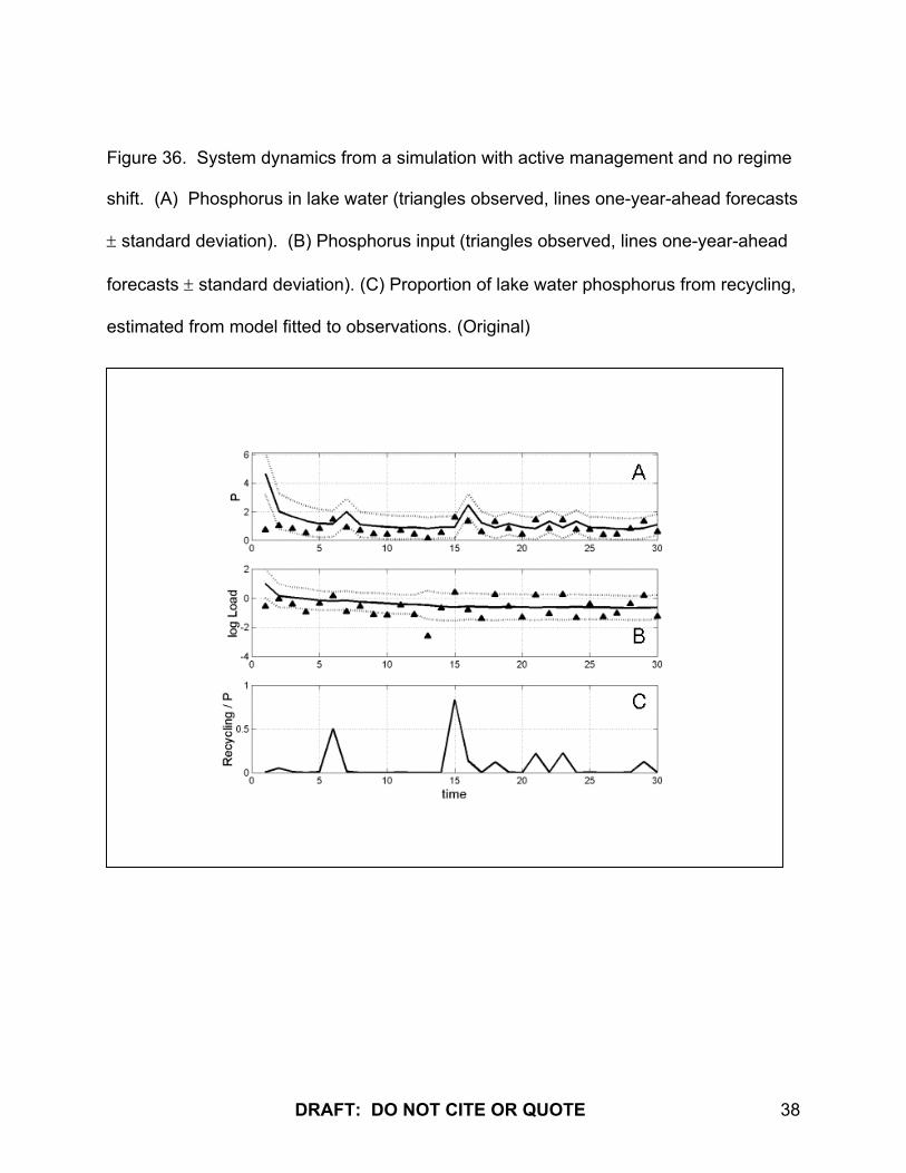
Figure 36. System dynamics from a simulation with active management and no regime
shift. (A) Phosphorus in lake water (triangles observed, lines one-year-ahead forecasts
± standard deviation). (B) Phosphorus input (triangles observed, lines one-year-ahead
forecasts ± standard deviation). (C) Proportion of lake water phosphorus from recycling,
estimated from model fitted to observations. (Original)
DRAFT: DO NOT CITE OR QUOTE 38

Figure 37. Interventions and parameter estimates from a simulation with active
management and no regime shift. (A) Management intervention as a proportion of
baseline phosphorus input. (B) – (D) show parameter estimates (crosses true but
unknown value, lines estimate ± standard deviation. (B) θ = 1 – (s+h) (C) ρ (D) η.
(Original)
DRAFT: DO NOT CITE OR QUOTE 39

Figure 38. System dynamics from a simulation with active management and a regime
shift. (A) Phosphorus in lake water (triangles observed, lines one-year-ahead forecasts
± standard deviation). (B) Phosphorus input (triangles observed, lines one-year-ahead
forecasts ± standard deviation). (C) Proportion of lake water phosphorus from recycling,
estimated from model fitted to observations. (Original)
DRAFT: DO NOT CITE OR QUOTE 40
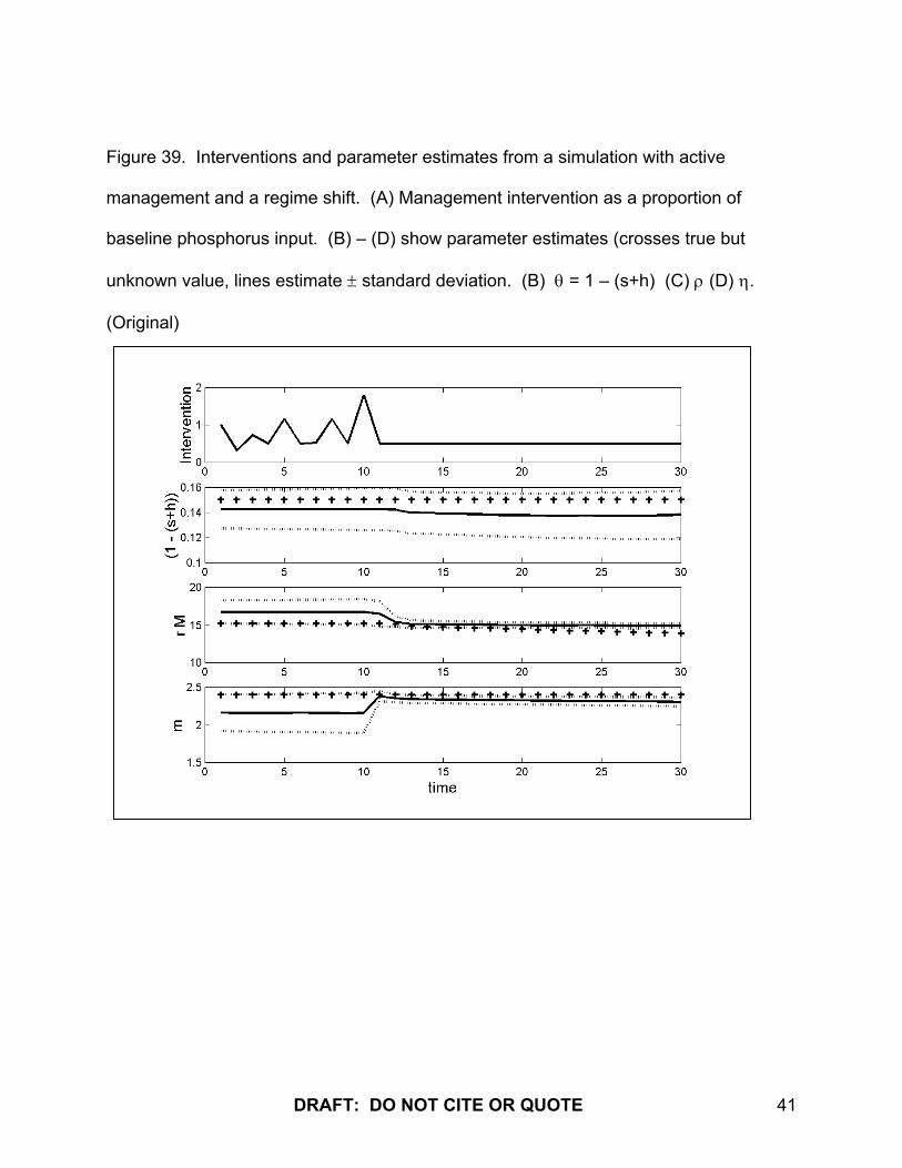
Figure 39. Interventions and parameter estimates from a simulation with active
management and a regime shift. (A) Management intervention as a proportion of
baseline phosphorus input. (B) – (D) show parameter estimates (crosses true but
unknown value, lines estimate ± standard deviation. (B) θ = 1 – (s+h) (C) ρ (D) η.
(Original)
DRAFT: DO NOT CITE OR QUOTE 41

Figure 40. (A) Bias in estimating maximum recycling rate r M (Estimated r M – true re
M) versus rank for simulations with passive management versus active management.
(B) Bias in estimating r M versus rank for simulations with or without a regime shift, and
with passive or active adaptive management. (Original)
DRAFT: DO NOT CITE OR QUOTE 42
Top Related