


Languages
Pages
Legal

USING ECONOMETRIC MODELS TO ANALYSE THE
SPATIAL DISTRIBUTION OF OIL PUMPKIN CULTIVATION IN
AUSTRIA
Andreas Niedermayr, Martin Kapfer and Jochen Kantelhardt
Andreas Niedermayr: [email protected]
Department of Economics and Social Sciences, University of Natural
Resources and Life Sciences, Vienna, Austria
2016
Copyright 2016 by authors. All rights reserved. Readers may make verbatim copies
of this document for non-commercial purposes by any means, provided that this
copyright notice appears on all such copies.
Paper prepared for presentation at the 56th annual conference of the
GEWISOLA (German Association of Agricultural Economists)
„Agricultural and Food Economy: Regionally Connected and Globally
Successful“
Bonn, Germany, September 28 – 30, 2016

2
USING ECONOMETRIC MODELS TO ANALYSE THE SPATIAL DISTRIBUTION OF OIL
PUMPKIN CULTIVATION IN AUSTRIA
Abstract
The liberalisation and globalisation of agricultural markets, has led to a shift of the EU
common agricultural policy from quantity based to quality based policies and is accompanied
by diversification of agricultural production in the European Union. For policy makers it is
therefore relevant to better understand the drivers that influence the adoption and spatial
distribution of emerging alternative practices and commodities in agriculture. Taking the
Styrian Oil Pumpkin as an example, the aim of this study is to quantify the drivers of spatial
variations in the cultivation of an emerging alternative crop. We estimate different
econometric models, drawing on cross sectional data of the year 2010 of 549 municipalities in
the Styrian Oil Pumpkin PGI area. Our findings indicate that (i) crop-specific factors,
(ii) region-specific factors and (iii) spatial interdependencies influence spatial variations in oil
pumpkin cultivated area and conclude that these factors also need to be considered for the
promotion of other emerging alternative practices and commodities in agriculture.
Keywords
Styrian Pumpkin Seed Oil, PGI, Austria, spatial econometrics, SLX model
1 Introduction
In recent decades the ongoing liberalisation and globalisation of agricultural markets has led
to an increasing exposure of agriculture in the European Union (EU) to competition on the
world market (THOMPSON et al., 2000; MCNAMARA and WEISS, 2005). One strategy to
confront this development is the diversification of agricultural production (MCNAMARA and
WEISS, 2005), which has led to a growing interest in alternative practices like organic farming
(DARNHOFER et al., 2005) or emerging alternative commodities like regional food products
(TREGEAR et al., 2007) and marks a shift of the EU common agricultural policy (CAP) from
quantity based to quality based policies (BECKER, 2009).
In the literature a wide range of factors has been identified that influence the adoption and
spatial distribution of alternative practices/commodities in agriculture. However, it is often
not considered that the relevant factors depend to a great extent on the specific crop/practice
as well as the regional context of the analysis (KNOWLER and BRADSHAW, 2007). For
example, adopting a crop is less complicated than adopting a practice like organic farming
that is not divisible and it takes longer until results of the adoption can be observed (PANNELL
et al., 2006). The regional context is relevant, because factors that facilitate the adoption of
the same practice or commodity may differ among regions due to region-specific potentials
(KNOWLER and BRADSHAW, 2007). Another important factor that is recognized in the
theoretical literature (PANNELL et al., 2006), but mostly not controlled for in empirical studies,
is spatial interdependence, meaning any form of strategic interaction, indirect effect or spatial
correlation among neighbouring observations. If spatial interdependence is not considered in
an empirical analysis, this can lead to biased results (STORM et al., 2015).
The aim of our study is therefore to analyse the drivers of spatial variations in the cultivation
of an emerging alternative crop, considering (i) crop-specific factors, (ii) region-specific
factors and (iii) spatial interdependence. For our analysis the cultivation of Styrian Oil
3
Pumpkin in Austria serves as an applied example. This has several reasons. Firstly, it is an
alternative crop that has experienced a very dynamic development in recent years. Secondly,
since 1996 the name “Styrian Pumpkin Seed Oil” is a protected geographical indication
(PGI), which limits the production of Styrian Pumpkin Seed Oil to a defined area (CRETNIK,
2014). Within this PGI area the cultivation of Styrian Oil Pumpkin is very unevenly
distributed and local agglomerations can be identified that may be related to spatial
interdependencies. Thirdly, the PGI area consists of two separated regions (northern and
southern part), which differ in terms of production and marketing structure and are therefore
likely to have developed in a different manner. Finally, to the best of our knowledge, no
previous study has analysed region-specific drivers of spatial variations of an alternative crop
with an empirical model.
As methodology we apply an econometric approach. This decision is based on the fact that we
have previously gained valuable information on possible drivers of oil pumpkin cultivation by
interviews with experts and now have access to a unique cross sectional dataset of the year
2010 for the 563 municipalities in the PGI area. To consider regional differences, we estimate
separate Tobit models for the northern and southern part of the PGI area. As a final step, we
control our results for the presence of spatial interdependencies by additionally estimating a
Spatial Lag of X (SLX) model, introduced by LESAGE (2009) and recently also advocated by
HALLECK VEGA and ELHORST (2015).
2 Background
2.1 Literature review of the adoption and spatial distribution of emerging practices
and commodities in agriculture
Having developed from the analysis of technology adoption (LINDNER, 1987), literature on
the adoption and spatial distribution of emerging practices and commodities in agriculture
comprises practices like organic farming (PADEL, 2001) or conservation agriculture
(RODRÍGUEZ-ENTRENA and ARRIAZA, 2013; ARSLAN et al., 2014) and commodities such as
switchgrass (JENSEN et al., 2007) or soy (GARRETT et al., 2013). In such studies data from
quantitative surveys or a farm census is analysed with either binary response (Probit/Logit) or
censored (Tobit/double-hurdle) regression models that quantify the influence of determinants
on the rate and/or intensity of adoption and spatial distribution of an emerging practice or
commodity. Frequently identified factors are for example farm size, farm profitability, bio-
physical quality of land or age and education level of the farmer among many others
(RODRÍGUEZ-ENTRENA and ARRIAZA, 2013).
With regard to spatial interdependence, several studies use spatial regression models to
analyse the spatial distribution of hog and dairy production (ROE et al., 2002; ISIK, 2004),
maize and soy cultivation (ODGAARD et al., 2011; GARRETT et al., 2013) or alternative
practices like organic farming (SCHMIDTNER et al., 2012; LÄPPLE and KELLEY, 2015;
SCHMIDTNER et al., 2015). For example GARRETT et al. (2013) analyse the determinants of
soybean cultivation in Brazil with a cross sectional spatial autoregressive (SAR) model on the
county level. Their main findings are that beneficial biophysical conditions that lead to higher
yields and certain supply chain configurations (cooperative membership and access to credit)
promote soybean cultivation. SCHMIDTNER et al. (2015) analyse spatial variations of organic
farming in the German federal states of Bavaria and Baden Württemberg on the municipality
and county level with a cross sectional SAR model. They find that less favourable climatic
conditions and a favourable social and political environment have a positive influence on
organic farming and conclude that the share of organic farms in a municipality/county also
depends on the share of organic farms in neighbouring municipalities or counties, which
implies the presence of spatial interdependence.
4
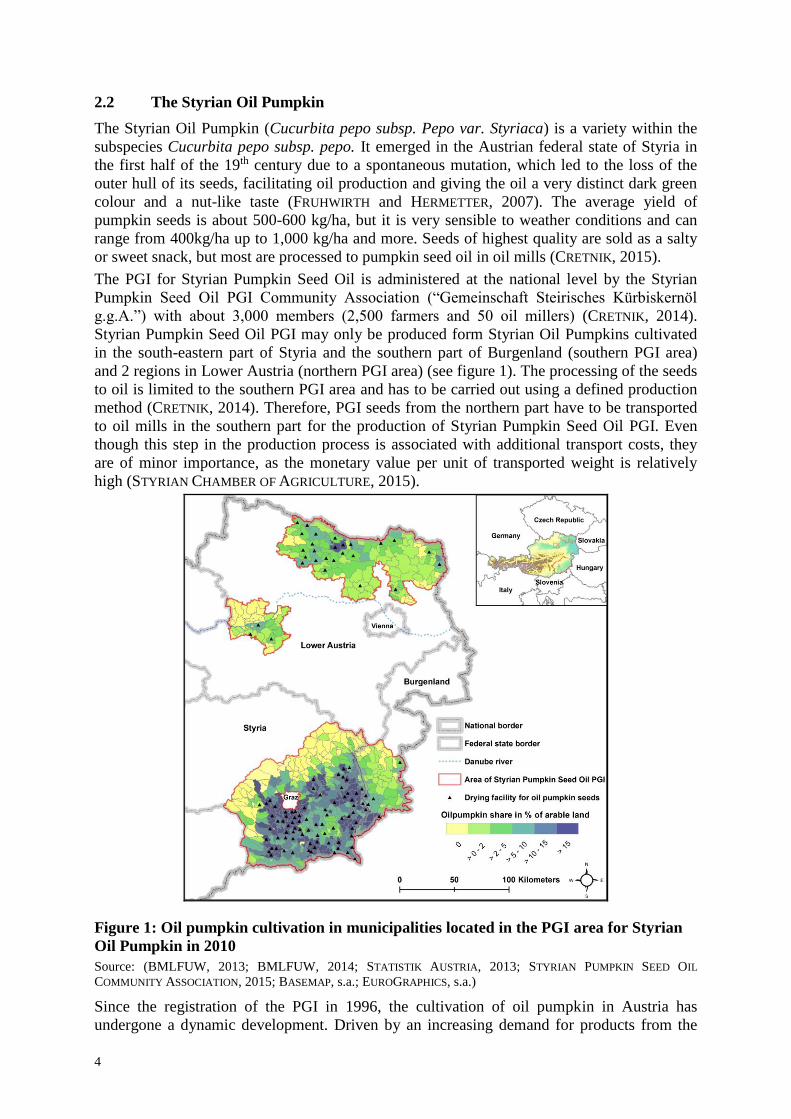
2.2 The Styrian Oil Pumpkin
The Styrian Oil Pumpkin (Cucurbita pepo subsp. Pepo var. Styriaca) is a variety within the
subspecies Cucurbita pepo subsp. pepo. It emerged in the Austrian federal state of Styria in
the first half of the 19th century due to a spontaneous mutation, which led to the loss of the
outer hull of its seeds, facilitating oil production and giving the oil a very distinct dark green
colour and a nut-like taste (FRUHWIRTH and HERMETTER, 2007). The average yield of
pumpkin seeds is about 500-600 kg/ha, but it is very sensible to weather conditions and can
range from 400kg/ha up to 1,000 kg/ha and more. Seeds of highest quality are sold as a salty
or sweet snack, but most are processed to pumpkin seed oil in oil mills (CRETNIK, 2015).
The PGI for Styrian Pumpkin Seed Oil is administered at the national level by the Styrian
Pumpkin Seed Oil PGI Community Association (“Gemeinschaft Steirisches Kürbiskernöl
g.g.A.”) with about 3,000 members (2,500 farmers and 50 oil millers) (CRETNIK, 2014).
Styrian Pumpkin Seed Oil PGI may only be produced form Styrian Oil Pumpkins cultivated
in the south-eastern part of Styria and the southern part of Burgenland (southern PGI area)
and 2 regions in Lower Austria (northern PGI area) (see figure 1). The processing of the seeds
to oil is limited to the southern PGI area and has to be carried out using a defined production
method (CRETNIK, 2014). Therefore, PGI seeds from the northern part have to be transported
to oil mills in the southern part for the production of Styrian Pumpkin Seed Oil PGI. Even
though this step in the production process is associated with additional transport costs, they
are of minor importance, as the monetary value per unit of transported weight is relatively
high (STYRIAN CHAMBER OF AGRICULTURE, 2015).
Figure 1: Oil pumpkin cultivation in municipalities located in the PGI area for Styrian
Oil Pumpkin in 2010
Source: (BMLFUW, 2013; BMLFUW, 2014; STATISTIK AUSTRIA, 2013; STYRIAN PUMPKIN SEED OIL
COMMUNITY ASSOCIATION, 2015; BASEMAP, s.a.; EUROGRAPHICS, s.a.)
Since the registration of the PGI in 1996, the cultivation of oil pumpkin in Austria has
undergone a dynamic development. Driven by an increasing demand for products from the

5
Styrian Oil Pumpkin, the arable land cultivated with oil pumpkin increased from about
9.000 ha in 1995 to approximately 32.000 ha in 2015. Farmers receive a higher price for
products that are produced according to the regulations of the PGI. Therefore, the vast
majority of oil pumpkin (roughly 90 percent) is cultivated in the PGI area (AMA, 2015).
Between 2000 and 2014 oil pumpkin cultivation within the PGI area increased in the northern
part from 1.700 to 8.200 ha and in the southern part from 8.500 to 13.700 ha (STATISTIK
AUSTRIA, 2015). The potential for oil pumpkin cultivation in these areas, considering crop
rotation limitations1, are 65.000 ha and 16.000 ha, respectively (CRETNIK, 2014).
3 Data basis and derivation of model variables
For our empirical model we draw on data from the municipality database (GEDABA)
(BMLFUW, 2013), the Integrated Administration and Control System (IACS) database
(BMLFUW, 2014), the Agricultural Structure Survey (STATISTIK AUSTRIA, 2013) and the
STYRIAN PUMPKIN SEED OIL COMMUNITY ASSOCIATION (2015). The analysis is carried out at
the municipality level, using cross sectional data from the year 2010 of the 563 municipalities
located in the Styrian Pumpkin Seed Oil PGI area. Before estimation of the models, several
observations are removed from the dataset, to reduce the effect of outliers and very small
municipalities in terms of arable land (less than 5 ha). After this step 549 municipalities
remain and represent the basis for our further analysis.
We now develop an overview of factors that may influence the spatial variations of oil
pumpkin cultivated area in the PGI area for Styrian Pumpkin Seed Oil. First, we define the
share of arable land cultivated with oil pumpkin as our dependent variable. In crop
production, different crops compete for a finite amount of arable land. The share of arable
land cultivated with a specific crop should therefore reflect its relative profitability, compared
to other crops (GARRETT et al., 2013) and to a certain extent also to livestock production
(depending on the amount of arable land that is required for the production of fodder). We
hypothesize that the relative profitability of oil pumpkin production in a cross sectional
setting with fixed price differences between competing crops depends on the natural quality
of arable land, access to special machinery required for oil pumpkin production, as well as
production- and marketing-related, political, social, spatial, temporal and regional factors,
which we describe subsequently in more detail. To limit the discussion on the broad range of
possible factors, we focus on variables that are available for our analysis.
The natural quality of arable land influences the yield potential. Moreover, pumpkins are not
frost tolerant and therefore require favourable climatic conditions during their vegetative
period from April to September, (DIEPENBROCK et al., 1999). We therefore introduce the soil
quality index of arable land (soilqual) as our first independent variable. It is an index number
that ranges from 0 to 100 and describes the quality of arable land, considering soil quality,
climatic conditions and topography.
While cultivation of oil pumpkins can be carried out with a precision drill, which is also used
for e.g. maize, other steps of the production process require special machinery. Pumpkin seed
harvesters pick up and crush the pumpkins and collect the seeds (HEYLAND et al., 2006). After
harvest, the seeds have to be washed and dried within a relatively short time frame
(approximately 6 hours) in stationary washing and drying facilities, to prevent them from
decay and prepare them for further processing (CRETNIK, 2015). Proximity to a washing and
drying facility for pumpkin seeds is therefore another prerequisite for oil pumpkin cultivation
and is introduced in our analysis with the variable distdry which measures the distance to the
next washing and drying facility in kilometres. As the machinery required for the harvest as
1 According to HEYLAND et al. (2006) due to phytopathological aspects, the share of oil pumpkin within crop
rotation should not exceed 25 percent.
6
well as for washing and drying is relatively expensive, these steps of the production process
are often carried out by agricultural service companies or organised collaboratively via
agricultural communities (BRANDSTETTER, 2014). We therefore include the variable agriserv
that indicates the amount of agricultural service provided to farms in working days.
The northern and southern part of the PGI area differ in terms of production and marketing
structure. The southern part is characterized by a very long tradition in oil pumpkin
cultivation, small farms and a high proportion of direct marketing farms (CRETNIK, 2014). In
the northern part farms are larger, oil pumpkin cultivation also has a certain tradition, but it is
not so important for regional identity and therefore direct marketing of pumpkin seed
products is also less prevalent. Still, in the northern PGI area the oil pumpkin is an interesting
crop for organic farms (BRANDSTETTER, 2014). Oil pumpkins are well suited to organic
farming, since after harvesting of the pumpkin seeds, the pulp mostly remains on the field and
provides nutrients for subsequent crops (Heyland et al., 2006). Moreover, a special product
line, “Organic Styrian Pumpkin Seed Oil PGI”, guarantees organic farms an additional price
premium. The farm size may have a positive or negative effect on oil pumpkin cultivation. It
can either facilitate investment into machinery or limit oil pumpkin production, as it is rather
labour intensive. To control for the effect of farm size in our model, we include the variable
farmsize, measured as utilized agricultural area (UAA) in ha per farm. The next variable,
share of organic farms per municipality (organic), should reflect the differing production and
marketing conditions of organic farms. To consider the different marketing possibilities of
direct marketing farms, we include the share of direct marketing farms (dirmark). The
competition with livestock production is considered by adding the variable livestock,
measured in livestock units per ha UAA.
Subsidies may be a political factor that influences spatial variations in oil pumpkin
cultivation. The UBAG-subsidy2 for example was granted for extensive land use practices on
arable land and grassland within the previous Austrian agri-environmental program. For
arable land, these practices included for example a wider crop rotation (less than 75% cereals
and maize) and low fertilizer input (BMLFUW, 2015). Therefore, this subsidy may have been
an incentive for farmers to cultivate oil pumpkin in order to widen their crop rotation. We
control for an effect of this subsidy with the variable (ubagarable) that measures the sum of
UBAG-subsidy in € granted for arable land per municipality.
In terms of social factors, the responsiveness of farmers to the dynamic development of oil
pumpkin cultivation in recent years may be relevant for explaining spatial variations in oil
pumpkin planted area. Literature shows that farmer characteristics like education or age and
the social environment often play a role in this context (e.g. LÄPPLE et al., 2015). For our
analysis we only have data on the education level of farmers, which we consider with the
variable education that describes the share of farmers with a higher agricultural education.
Within the agricultural structure survey this is defined as an agricultural education that
comprises at least 3 years (STATISTIK AUSTRIA, 2013).
Finally, temporal and regional aspects also play a crucial role. For example, historical factors
like a longer tradition in oil pumpkin cultivation may also influence current differences in oil
pumpkin shares. To consider such unobserved heterogeneity among municipalities in a cross
sectional analysis with aggregated data, a temporal lag of the dependent variable (mean of the
oil pumpkin share of 2000 and 2001) is included as a control (oilplag), a procedure proposed
by WOOLDRIDGE (2012). Another control variable is the arable land per municipality (arable),
which allows us to estimate the share of oil pumpkin cultivated area of arable land, while
holding arable land constant. A simple way to consider regional differences in a regression
model is to include regional dummy variables. However, if the effects of the independent
variables differ among regions, which is what we hypothesise in this analysis, this can be
2 UBAG is an abbreviation for environmentally friendly management of arable land and grassland.

7
addressed by estimating separate regression models for the regions (northern and southern
PGI area). For the analysis the variables farmsize, ubagarable and arable were logarithmized
to approximate a normal distribution and reduce the effect of outliers (WOOLDRIDGE, 2012).
An overview of the variables used in our regression models is given in Table 1. A major
pattern that can be observed is that means of most variables differ considerably between the
two regions. Next to the description of the independent variables, we include the hypothesized
sign of the independent variables.
Table 1: Descriptive statistics
Category Variable
(Hypothesized sign) Code Unit
Northern
PGI area
(n = 143)
Southern
PGI area
(n = 406)
Dependent
variable
Share of oil pumpkin in percent of arable
land (dependent variable) oilp % 2.3 10.7
Natural Soil quality index of arable land (+) soilqual index 51.5 42.5
Machinery Distance to next washing/drying facility
(-) distdry km 4.0 4.2
Machinery Agricultural service per farm (+) agriserv days/farm 1.0 0.8
Production Farm size (+/-) farmsize ha UAA 36.2 12.7
Production Share of organic farms (+) organic % 11.8 9.0
Production Livestock density (-) livestock LU/ha 0.4 1.0
Political UBAG-subsidy for arable land (+) ubagarable € 120,150.3 13,671.8
Marketing Share of farms with direct marketing (+) dirmark % 4.5 7.5
Social Share of farmers with higher agricultural
education (+) education % 33.9 17.1
Control Arable land (+) arable ha 1.928.6 413.1
Control Temporal lag of oil pumpkin share
(mean of 2000 and 2001) (+) oilplag % 0.6 5.4
Note: Values are means; UAA = utilized agricultural area; LU = livestock unit
Source: Various sources given in the text.
4 Econometric model
As the share of oil pumpkin cultivated area is zero in roughly 20% of the observed
municipalities, estimation of a linear model, estimated by ordinary least squares would lead to
biased results due to censoring (WOOLDRIDGE, 2012). We address this issue by estimating a
Tobit model that takes censoring into account and is often applied in similar studies (e.g.
CONSMÜLLER et al., 2010; JENSEN et al., 2007; LANGYINTUO and MEKURIA, 2008). The Tobit
model expresses the dependent variable Y of a linear regression model in combination with an
underlying latent variable Y* (WOOLDRIDGE, 2012)
(1)
, where Y* equals Y if it takes on a value greater than 0, but it takes on a negative value if Y
is zero. is a constant term, is a vector of k regression coefficients, X is a matrix with the n
values of the k independent variables and U is a vector of n normally distributed errors. In
contrast to an ordinary least squares regression, the partial effect of an independent variable
(X) on the dependent variable (Y) in a Tobit model varies with the values of X. We therefore
use the partial effect at the average (PEA) which expresses the effect of X on Y when all X
are evaluated at their mean values. The PEA can be interpreted in the same way as the
regression coefficients from an OLS regression and is calculated by multiplying Tobit
coefficients with the following adjustment factor (WOOLDRIDGE, 2012):
(2)

8
In a second step, we control our results for the existence of spatial interdependence. Basically,
spatial interdependence can be introduced into a regression model either through global or
local spillover effects. Local spillover effects are present, if a change in a characteristic of an
observation affects the outcome of neighbouring observations. Global spillover effects on the
other hand imply that a change in a characteristic/outcome of one observation influences the
outcome of all observations in the sample, ultimately leading to endogenous feedback effects
(LESAGE, 2014). In the literature, in most empirical applications statistical tests are used to
choose between competing model specifications, which are very often the spatial
autoregressive (SAR) model that produces global spillover effects and the spatial error (SEM)
model, which filters spatial correlation out of the error term to provide unbiased standard
errors of estimates, but does not produce spillover effects.
This procedure is common in applied econometrics (see e.g. ANSELIN, 2010) and has also
found broader acceptance in an agricultural context (e.g. ROE et al., 2002; SCHMIDTNER et al.,
2012; or HOLLOWAY et al., 2007 for a broader review), but has recently also been object to
growing criticism. Specifically, GIBBONS and OVERMAN (2012) argue that most applied
spatial econometric research is bedevilled by identification problems of the causal
relationships at work and has too much focus on statistical tests when determining the
appropriate model specification. Instead of the mainly used SAR and SEM models, they
advocate the use of the simpler Spatial Lag of X (SLX) model, first introduced by LESAGE
(2009), which produces local spillover effects and call for more focus on theoretical
considerations and precisely defined research questions, when analysing spatial
interdependence. In response to this criticism HALLECK VEGA and ELHORST (2015) also
propose the SLX model as a point of departure, when controlling for spatial interdependence.
Simply put, local spillovers offer a more flexible way to model spillovers, impose less
restrictions in terms of model assumptions and are also more likely in the majority of cases
(LESAGE, 2014; HALLECK VEGA and ELHORST, 2015). For example, in the SLX model
spillover effects may differ for every independent variable to an extent that they can even take
on different signs, whereas in the SAR model the ratio between direct and spillover effects is
by definition constant for all variables and the spillover effects have the same sign as direct
effects, which is a rather restrictive and undesirable property (Pace and Zhu, 2012). We
therefore consider local spillover effects to be more flexible and also more credible, when
considering their possible influence on spatial variations in the cultivation of alternative crops
like the oil pumpkin.
(3)
, where W is a N x N neighbourhood matrix, often based on continuous neighbourhood for
administrative units. In a continuous neighbourhood matrix, observations which share a
border are neighbours and receive the value 1, all other observations receive the value 0.
Additionally, the diagonal elements of the matrix are also 0, as an observation cannot be a
neighbour of itself. Before estimation of the model, the neighbourhood matrix has to be row
standardized, so that all rows sum up to 1. The result of the multiplication of X with W is a
spatial lag variable that represents the average X value of neighbouring observations. In the
SLX model, the PEA of β measures the direct effects of X on Y, while the PEA of γ measures
local spillover effects of WX on Y. If the PEA of γ is statistically significant, local spatial
interdependence is present.
To test the robustness of our model specification, we estimate all models with 2 different
neighbourhood matrices, one based on continuous neighbourhood and one based on a cut-off
distance of 10 kilometres (euclidean distance between geographic centroid points of
municipalities), where neighbours are additionally weighted according to their inverse
distance. The decision for the cut-off distance is based on expert knowledge regarding the
structure of the oil pumpkin market in Austria and on comparison with other work that
analysed spatial interdependencies in agriculture (SCHMIDTNER et al., 2015). However, as the

9
results of both specifications do not differ substantially, we only present the results based on
the continuous neighbourhood matrix.
5 Results
The results of the estimated regression models are provided in Table 2. To enable direct
interpretation of the effects of the independent variables on the share of arable land cultivated
with oil pumpkin, the PEAs are presented instead of the estimated coefficients. Overall, most
signs of the PEAs are in line with their hypothesized effect on the share of arable land
cultivated with oil pumpkin. In regard to the spatial models, the results do not differ
substantially from the non-spatial models. We therefore focus mainly on the PEAs of the
Tobit model for interpretation of the results and only refer to the PEAs of the SLX Tobit
model, when differences arise. In the SLX Tobit models, we only include spatial lags of the
variables dirmark, organic, agriserv and education. The two variables arable and oilplag are
not included as spatial lags, because they primarily serve as controls and therefore it is of no
interest to interpret their marginal effects. The other independent variables are not included as
spatial lags, because the high correlation with their spatial lags (WX) does not allow us to
identify their marginal effects3.
In the model for the northern PGI area, soilqual, organic, education and oilplag have a
positive and statistically significant effect, even though for education it is only significant in
the SLX Tobit model. With regard to the variable oilplag it has to be considered that the
primary purpose of this variable is not to interpret its partial effect, but rather to control for
unobservable heterogeneity that influences oil pumpkin shares. Next, the variables distdry,
farmsize and dirmark show a statistically significant and negative effect. For example, one
additional kilometre to the next washing and drying facility, is on average associated with a
decrease of oil pumpkin cultivation by 0.25 percentage points. Finally, none of the spatial lag
variables in the SLX Tobit model is statistically significant in the northern PGI area, which
means that no local spatial interdependencies are present in the northern PGI area.
Moving on to the southern PGI area, the variables soilqual, ubagarable, dirmark and oilplag
show a positive and statistically significant influence on oil pumpkin shares, while the effect
of distdry, farmsize and livestock is negative and statistically significant. Note that livestock
was multiplied by 10 to facilitate interpretation of its PEA. An increase of 0.1 livestock units
per ha UAA is therefore associated with a decrease of oil pumpkin share by 0.24 percentage
points. In comparison to the northern PGI area the effects of soilqual farmsize, organic,
livestock, ubagarable, dirmark and oilplag differ. The effects of soilqual and farmsize are
bigger and shows a higher significance level. Organic farming has no significant effect on oil
pumpkin shares and the negative effect of livestock is higher and significant (1%-level). Next,
UBAG payments for arable land have a positive and statistically significant effect on oil
pumpkin shares in the southern PGI area, even though it is only significant at the 5% level in
the Tobit model. Another region specific aspect is the positive effect (0.17) of direct
marketing on oil pumpkin shares in the southern PGI area (significant at the 1% level). As in
the northern PGI area, the control variable arable has no statistically significant effect on oil
pumpkin shares. This means that oil pumpkin shares are independent from the size of the
municipality in terms of arable land. Finally, the spatial lag variable W.dirmark has a positive
and statistically significant effect (1% level) on oil pumpkin shares. An increase of the
average direct marketing share of neighbouring municipalities by 1 percentage point, is
therefore associated with an increase of the oil pumpkin share in a municipality by 0.26
percentage points.
3 A similar problem occurred in the work of STORM et al. (2015), which also led them to exclude certain spatial
lag variables from their analysis.

10
Table 2: PEAs of Tobit and SLX Tobit models for northern and southern PGI area
PEA Northern PGI area (n =143) Southern PGI area (n = 406)
Tobit SLX Tobit Tobit SLX Tobit
Direct effects:
soilqual 0.04* 0.05* 0.32*** 0.32***
distdry -0.25*** -0.26*** -0.52*** -0.48***
agriserv 0.10 n.s. 0.09 n.s. -0.02 n.s. -0.03 n.s.
log(farmsize) -0.01* -0.01** -0.03*** -0.03***
organic 0.09*** 0.09*** 0.02 n.s. 0.02 n.s.
livestock -0.08 n.s. -0.07 n.s. -0.24*** -0.26***
log(ubagarable 0.002 n.s. 0.003 n.s. 0.003** 0.002 n.s.
dirmark -0.07* -0.07* 0.17*** 0.13***
education 0.02 n.s. 0.03* -0.01 n.s. -0.01 n.s.
log(arable) 0.0006 n.s. 0.0001 n.s. -0.002 n.s. -0.001 n.s.
oilplag 1.05*** 1.04*** 0.82*** 0.78***
Local spillover effects:
W.agriserv 0.10 n.s. -0.11 n.s.
W.organic -0.01 n.s. 0.02 n.s.
W.dirmark -0.10 n.s. 0.26***
W.education -0.02 n.s. -0.01 n.s.
Note: the PEAs of the 3 log-transformed independent variables have been divided by 100 so that a change of x
by 1% can be interpreted as a percentage point change of y. Spatial lag variables are denoted by the prefix “W.”
***, ** and * and denote significance at the 1%, 5% and 10% levels, respectively; n.s. = not significant.
6 Discussion and conclusions
In our study we estimate different regression models to analyse the potential drivers of spatial
variations in oil pumpkin cultivation within the Styrian Oil Pumpkin PGI area. To allow for
region-specific effects in the northern and southern part of the PGI area, we separately
estimate one regression model for each region, using the same set of variables for both
models. Additionally, we control our results for the presence of possible local spatial
interdependence, by estimating a SLX model, leading to a total of 4 regression models.
Starting with overall aspects, the positive effect of natural conditions is plausible and in line
with the results of other studies that carried out such analysis for crops with similar climatic
requirements, namely maize and soybean (ODGAARD et al., 2011; GARRETT et al., 2013). Also
not surprising is the great extent by which historical factors explain spatial variations in oil
pumpkin cultivated area. However, including this variable in the analysis allows us to
measure the effects of the other independent variables, while holding historical factors, like a
longer tradition or more experience with oil pumpkin cultivation and other unobservable
factors constant (WOOLDRIDGE, 2012). Proximity to a washing and drying facility is also
important for oil pumpkin cultivation. Even though we are able to quantify a negative effect
of distance to the next washing and drying facility, a remaining shortcoming of our analysis is
that we could not include the actual capacity of the washing and drying facilities in our model
due to lack of data. Somewhat surprising is the negative effect of farm size on oil pumpkin
shares. In the southern PGI area this may be explained in combination with the high share of
direct marketing farms, whereas in the northern PGI area, organic farms, which are generally
smaller in terms of UAA, are more likely to cultivate oil pumpkin.
Additionally, we are also able to identify region-specific factors that influence spatial
variations in oil pumpkin cultivation. In the northern PGI area, the drier climate results in a
lower yield potential, making organic farming more attractive. Thus, the positive effect of
11
organic farming on oil pumpkin cultivation may reflect the good suitability of oil pumpkins
for organic farming in this region.
In the southern PGI area the positive effect of direct marketing confirms the hypothesis of
direct marketing as an important regional sales channel for oil pumpkin products. This
regional importance may be explained by the smaller farm structure in combination with the
long tradition with and therefore also strong contribution to regional identity by the Styrian
Oil Pumpkin. The negative relationship between livestock production and oil pumpkin
cultivation in the southern PGI area is likely to be based on a different orientation of
agricultural production. While farmers in the northern PGI area mainly focus on cash crops,
livestock production plays an important role for farmers in the southern PGI area. However, it
cannot be clearly confirmed, whether the negative effect of livestock density arises due to
competition (e.g. with hog production) or less suitability of oil pumpkin cultivation (negative
correlation of oil pumpkin shares with grassland shares). A reason for the positive effect of
UBAG payments could be that farmers in the southern PGI have a more cereal and maize
dominated crop rotation and mostly extended their production to soybean or oil pumpkin,
when they participated in the UBAG subsidy. On the contrary, farmers in the northern PGI
area have a broader crop rotation, including for example sugar beet, sun flower or rape, which
also explains the higher UBAG payments received in the northern PGI area, despite the lower
oil pumpkin shares.
Finally, higher shares of direct marketing farms in neighbouring municipalities are associated
with a higher share of oil pumpkin cultivated area. This local spatial interdependence may
have different meanings. Firstly, more direct marketing in a neighbourhood could attract more
potential customers, as it bundles supply and therefore leads to an increase of oil pumpkin
cultivation. Secondly, like for the other independent variables, it is possible that the PEA of
the variable W.dirmark simply describes correlation of neighbouring direct marketing shares
with oil pumpkin shares and no marginal effect. As also stated in STORM et al. (2015), it is not
possible to empirically assess, through which of the above described channels spatial
interdependence arises.
Another shortcoming due to lack of data is that we were only able to carry out the analysis at
the municipality level. This aggregated data may lead to the ecological fallacy problem
(ANSELIN, 2002) and the modifiable areal unit problem (OPENSHAW, 1984), meaning that
results from (artificially) aggregated data may be different or even reverse compared to the
level on which economic agents (farmers) act. In a spatial econometric context, the
aggregation of data may also lead to artificial spatial interdependence. Even though
SCHMIDTNER et al. (2015) show that previously found evidence for spatial interdependence in
organic farming in Germany on the county level, also holds at the municipality level, these
aspects have to be considered, when interpreting our results. Another issue is that our results
are only valid for a given point in time (the year 2010). Even though we control for historical
unobservable factors by introducing a temporal lag variable into our model, an analysis with
panel data would enable us to consider the temporal dynamics of spatial variations in oil
pumpkin cultivated area in the PGI area and is therefore considered as a promising venue for
future research, given data availability.
The conclusions that can be drawn from our results apply on a more general level also to
other emerging practices or commodities in agriculture, as they point out that (i) practice- or
commodity-specific, (ii) region-specific and (iii) spatial aspects need to be considered by
policy makers, for the promotion of alternatives in agriculture. Like KNOWLER and
BRADSHAW (2007) argue, researchers in this area should therefore pay increased attention to
the thematic and regional context of their analysis instead of focussing on “universal” factors.
Additionally, we recommend to control for spatial interdependence, as otherwise results may
be biased.
12
Literature
AMA, (Agrarmarkt Austria) (2015): Getreideanbauflächen in Österreich 2005-2015.
ANSELIN, L. (2002): Under the hood: issues in the specification and interpretation of spatial regression
models. Agricultural economics 27 (3): 247-267.
ANSELIN, L. (2010): Thirty years of spatial econometrics. Papers in Regional Science 89 (1): 3-25.
ARSLAN, A., MCCARTHY, N., LIPPER, L., ASFAW, S. and CATTANEO, A. (2014): Adoption and
intensity of adoption of conservation farming practices in Zambia. Agriculture, Ecosystems &
Environment 187: 72-86.
BASEMAP (s.a.): Topographic map of Austria. www.basemap.at [02.2016].
BECKER, T. C. (2009): European Food Quality Policy: The Importance of Geographical Indications,
Organic Certification and Food Quality Assurance Schemes in European Countries. Estey
Centre Journal of International Law and Trade Policy 10 (1).
BMLFUW, (Federal Ministry of Agriculture, Forestry, Environment and Water Management) (2013):
Municipality Database. Unpublished.
BMLFUW, (Federal Ministry of Agriculture, Forestry, Environment and Water Management) (2014):
Integrated Administration and Control System Database. Unpublished.
BMLFUW, (Federal Ministry of Agriculture, Forestry, Environment and Water Management) (2015):
ÖPUL 2007 Übersicht. https://www.bmlfuw.gv.at/land/laendl_entwicklung/le-07-13/agrar-
programm/OEPUL-Uebersicht.html [12.2015].
BRANDSTETTER, A. (2014): Interview about the cultivation of Styrian Oil Pumpkin and the production
of Styrian Pumpkin Seed Oil PGI.
CONSMÜLLER, N., BECKMANN, V. and PETRICK, M. (2010): An econometric analysis of regional
adoption patterns of Bt maize in Germany. Agricultural economics 41 (3-4): 275-284.
CRETNIK, A. (2014): Interview about the cultivation of Styrian Oil Pumpkin and the production of
Styrian Pumpkin Seed Oil PGI.
CRETNIK, A. (2015): Personal comunication regarding harvest, processing and use of oil pumpkin
seeds.
DARNHOFER, I., SCHNEEBERGER, W. and FREYER, B. (2005): Converting or not converting to organic
farming in Austria: Farmer types and their rationale. Agriculture and Human Values 22 (1):
39-52.
DIEPENBROCK, W., FISCHBECK, G. and HEYLAND, K. U. (1999): Spezieller Pflanzenbau. Stuttgart,
UTB Ulmer.
EUROGRAPHICS (s.a.): Worldwide national borders of 2014.
http://ec.europa.eu/eurostat/cache/GISCO/geodatafiles/CNTR_2014_03M.zip [02.2016].
FRUHWIRTH, G. O. and HERMETTER, A. (2007): Seeds and oil of the Styrian oil pumpkin: Components
and biological activities. European Journal of Lipid Science and Technology 109 (11): 1128-
1140.
GARRETT, R. D., LAMBIN, E. F. and NAYLOR, R. L. (2013): Land institutions and supply chain
configurations as determinants of soybean planted area and yields in Brazil. Land Use Policy
31: 385-396.
GIBBONS, S. and OVERMAN, H. G. (2012): Mostly pointless spatial econometrics? Journal of Regional
Science 52 (2): 172-191.
HALLECK VEGA, S. and ELHORST, J. P. (2015): The SLX model. Journal of Regional Science 55 (3):
339-363.
HEYLAND, K. U., HANUS, H. and KELLER, E. R. (2006): Ölfrüchte, Faserpflanzen, Arzneipflanzen und
Sonderkulturen. Ulmer.
HOLLOWAY, G., LACOMBE, D. and LESAGE, J. P. (2007): Spatial Econometric Issues for Bio-
Economic and Land-Use Modelling. Journal of Agricultural Economics 58 (3): 549-588.
ISIK, M. (2004): Environmental Regulation and the Spatial Structure of the U.S. Dairy Sector.
American Journal of Agricultural Economics 86 (4): 949-962.
JENSEN, K., CLARK, C. D., ELLIS, P., ENGLISH, B., MENARD, J., WALSH, M. and DE LA TORRE
UGARTE, D. (2007): Farmer willingness to grow switchgrass for energy production. Biomass
and Bioenergy 31 (11–12): 773-781.
KNOWLER, D. and BRADSHAW, B. (2007): Farmers’ adoption of conservation agriculture: A review
and synthesis of recent research. Food Policy 32 (1): 25-48.
13
LANGYINTUO, A. S. and MEKURIA, M. (2008): Assessing the influence of neighborhood effects on the
adoption of improved agricultural technologies in developing agriculture. African Journal of
Agricultural and Resource Economics 2 (2): 151-169.
LÄPPLE, D. and KELLEY, H. (2015): Spatial dependence in the adoption of organic drystock farming in
Ireland. European Review of Agricultural Economics 42 (2): 315-337.
LÄPPLE, D., RENWICK, A. and THORNE, F. (2015): Measuring and understanding the drivers of
agricultural innovation: Evidence from Ireland. Food Policy 51: 1-8.
LESAGE, J. P. (2009): Introduction to Spatial Econometrics. Boca Raton, CRC Press.
LESAGE, J. P. (2014): What Regional Scientists Need to Know about Spatial Econometrics. The
Review of Regional Studies 44 (1): 13-32.
LINDNER, R. K. (1987): Adoption and diffusion of technology: an overview. In B. R. Champ, E.
Highly, J. V. Remenyi (eds), Technological Change in Postharvest Handling and
Transportation of Grains in the Humid Tropics. Canberra, Australian Centre for International
Agricultural Research.
MCNAMARA, K. and WEISS, C. (2005): Farm Household Income and On- and Off-Farm
Diversification. Journal of agricultural and applied economics 37 (1): 37-48.
ODGAARD, M. V., BØCHER, P. K., DALGAARD, T. and SVENNING, J.-C. (2011): Climatic and non-
climatic drivers of spatiotemporal maize-area dynamics across the northern limit for maize
production: A case study from Denmark. Agriculture, Ecosystems & Environment 142 (3–4):
291-302.
OPENSHAW, S. (1984): The modifiable areal unit problem. Norwich, Geo Books.
PADEL, S. (2001): Conversion to Organic Farming: A Typical Example of the Diffusion of an
Innovation? Sociologia Ruralis 41 (1): 40-61.
PANNELL, D. J., MARSHALL, G. R., BARR, N., CURTIS, A., VANCLAY, F. and WILKINSON, R. (2006):
Understanding and promoting adoption of conservation practices by rural landholders.
Australian Journal of Experimental Agriculture 46 (11): 1407-1424.
RODRÍGUEZ-ENTRENA, M. and ARRIAZA, M. (2013): Adoption of conservation agriculture in olive
groves: Evidences from southern Spain. Land Use Policy 34: 294-300.
ROE, B., IRWIN, E. G. and SHARP, J. S. (2002): Pigs in space: modeling the spatial structure of hog
production in traditional and nontraditional production regions. American Journal of
Agricultural Economics 84 (2): 259-278.
SCHMIDTNER, E., LIPPERT, C. and DABBERT, S. (2015): Does Spatial Dependence Depend on Spatial
Resolution? – An Empirical Analysis of Organic Farming in Southern Germany. German
Journal of Agricultural Economics 64 (3): 175-191.
SCHMIDTNER, E., LIPPERT, C., ENGLER, B., HÄRING, A. M., AURBACHER, J. and DABBERT, S. (2012):
Spatial distribution of organic farming in Germany: does neighbourhood matter? European
Review of Agricultural Economics 39 (4): 661-683.
STATISTIK AUSTRIA (2013): Farm census 2010.
STATISTIK AUSTRIA (2015): Feldfrucht- und Dauerwiesenproduktion, endgültiges Ergebnis 2014.
https://www.statistik.at/web_de/statistiken/wirtschaft/land_und_forstwirtschaft/agrarstruktur_f
laechen_ertraege/feldfruechte/080350.html [09.2015].
STORM, H., MITTENZWEI, K. and HECKELEI, T. (2015): Direct Payments, Spatial Competition, and
Farm Survival in Norway. American Journal of Agricultural Economics 97 (4): 1192-1205.
STYRIAN CHAMBER OF AGRICULTURE (2015): Steirischer Marktbericht Nr. 38 zum 17. September
2015.
STYRIAN PUMPKIN SEED OIL COMMUNITY ASSOCIATION (2015): Data of locations of washing and
drying facilities and oil mills. Unpublished.
THOMPSON, S. R., ROLAND, H. and GOHOUT, W. (2000): Agricultural Market Liberalization and
Instability of Domestic Agricultural Markets: The Case of the CAP. American Journal of
Agricultural Economics 82 (3): 718-726.
TREGEAR, A., ARFINI, F., BELLETTI, G. and MARESCOTTI, A. (2007): Regional foods and rural
development: The role of product qualification. Journal of Rural Studies 23 (1): 12-22.
WOOLDRIDGE, J. (2012): Introductory econometrics: A modern approach. Cengage Learning.
Top Related