


Languages
Pages
Legal

USER’S GUIDE TO GALOPER - A PROGRAM FOR
SIMULATING THE SHAPES OF CRYSTAL SIZE
DISTRIBUTIONS - AND ASSOCIATED PROGRAMS
_________________________________________________________
U.S. Geological Survey
Open-File Report: OF 00-505___________________________________________________________
_

2
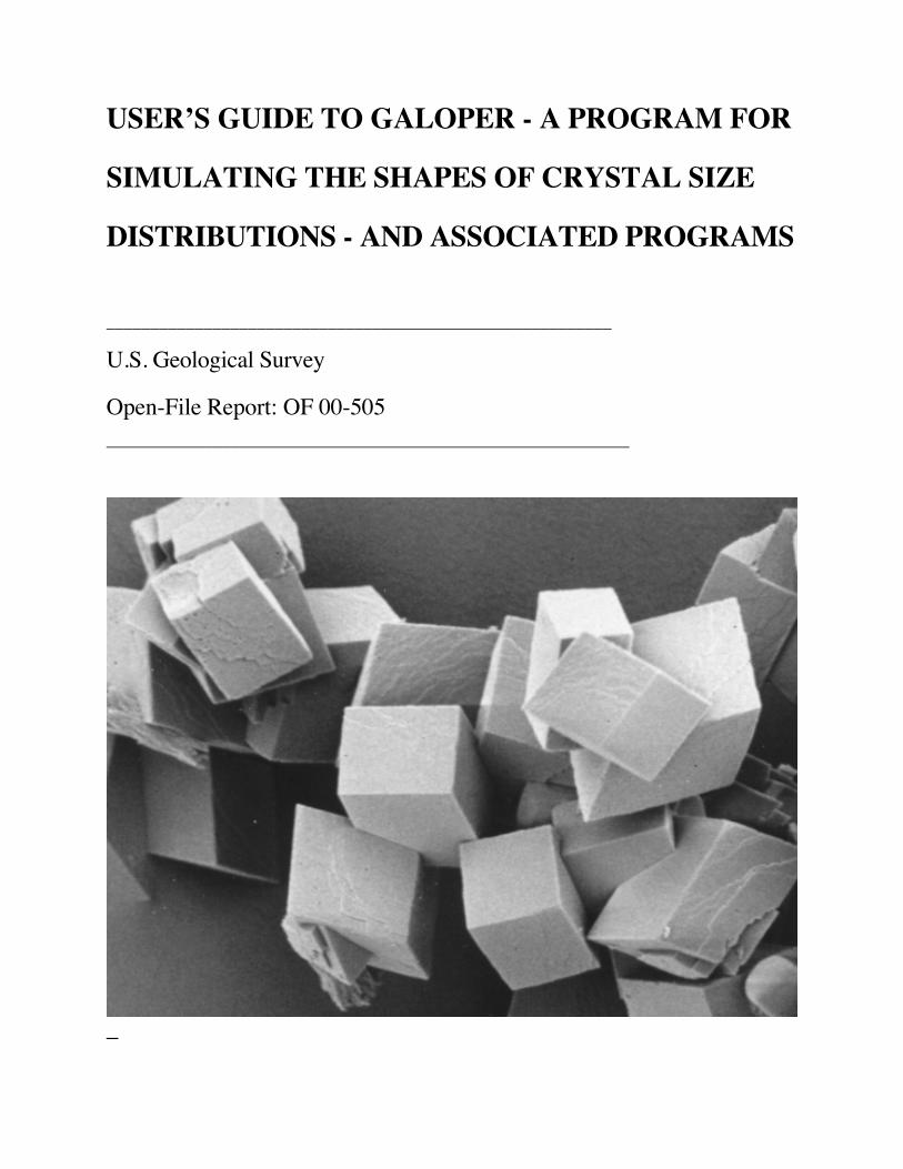
Cover photo: Scanning electron micrograph (SEM) of synthetic calcite crystals that haveundergone Ostwald ripening, followed by supply-controlled growth. The mean crystaldiameter is 6.2 micrometers. Photo by Dan Kile, US Geological Survey.
3
U.S. DEPARTMENT OF THE INTERIORBRUCE BABBITT, SecretaryU.S. GEOLOGICAL SURVEYCharles G. Groat, Director
The use of trade, product or firm names is for descriptive purposes only and does not implyendorsement by the U.S. Government.
RTS-ID Number R2-0589
Boulder, Colorado
12/18/2000
For additional information, to:
Chief, Branch of Regional ResearchU.S. Geological SurveyBox 25046, MS 418Denver Federal CenterDenver, CO 80225
4
CONTENTS
Page
Poems by Wallace Stevens……………………………………………………………………. 5
Abstract…………………………………………………………………………………………6
Introduction…………………………………………………………………………………… 6
Computer requirements……………………………………………………………….. 7
How to obtain programs………………………………………………………………. 8
Installation of programs………………………………………………………………. 9
Use of GALOPER……………………………………………………………………………. 9
Crystal growth in open systems………………………………………………………. 10
Crystal growth in closed systems …………………………………………………….. 16
Iteration during simulation of Ostwald ripening………………………………………. 21
Use of Associated Programs…………………….……………………………………………. 22
Simulation Examples………………………………………………………………………….. 24
References…………………………………………………………………………………….. 33
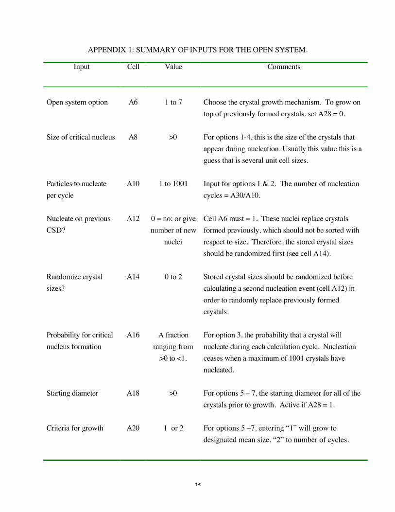
Appendix 1: Summary of Inputs for Open System……………………………………………. 35
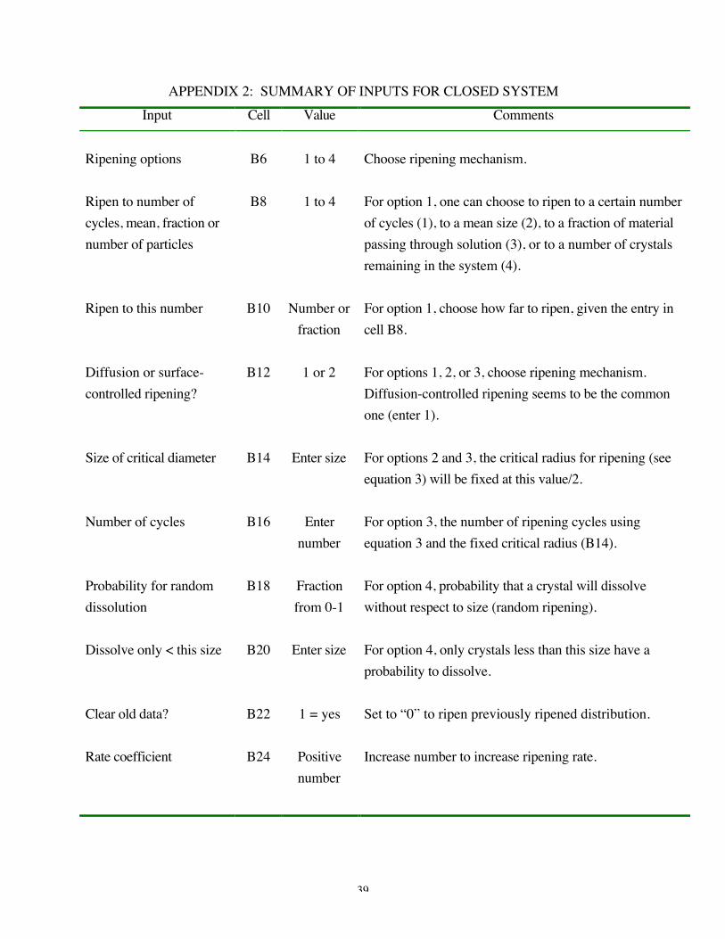
Appendix 2: Summary of Inputs for Closed System …………………………………………. 39
Appendix 3: Summary of Results for Open System………………………………………….. 42
Appendix 4: Summary of Results for Closed System ………………………………………… 43
Figures: 1. Sample inputs for open system………………………………………………… 19
2. Sample inputs for closed system………………………………………………. 20
3. Graphs showing three basic shapes for crystal size distributions……………… 26
4. Graphs showing an α−β2 diagram of the reaction path for an illite sample……. 31
5. Graph showing simulated and measured crystallite thickness distribution for an illite
Sample………………………………………………………………………… 32
Table 1. How subsequent crystal growth mechanisms may change the initial shapes of crystal size
distributions (CSDs)………………………………………………………………….. 28

5
POEMS BY WALLACE STEVENS
From “CONNOISSEURS OF CHAOS”
A. A violent order is disorder; and
B. A great disorder is an order. These
Two things are one. (Pages of illustrations.)
From “THE PLEASURES OF MERELY CIRCULATING”
The garden flew round with the angel,
The angel flew round with the clouds,
And the clouds flew round and the clouds flew round
And the clouds flew round with the clouds.
6
USER’S GUIDE TO GALOPER - A PROGRAM FOR SIMULATING THE SHAPES OF
CRYSTAL SIZE DISTRIBUTIONS - AND ASSOCIATED PROGRAMS
By D. D. Eberl1, V. A. Drits2, and J. Írodo~3
1U.S. Geological Survey, 3215 Marine St., Boulder, CO 80303-1066 USA;2Institute of Geology RAN. Pyzevskij 7, 109017 Moscow, Russia;
3Institute of Geological Sciences PAN, Senacka 1, 31002 Krakow, Poland.
ABSTRACT
GALOPER is a computer program that simulates the shapes of crystal size distributions
(CSDs) from crystal growth mechanisms. This manual describes how to use the program. The
theory for the program’s operation has been described previously (Eberl, Drits, and Írodo~, 1998).
CSDs that can be simulated using GALOPER include those that result from growth mechanisms
operating in the open system, such as constant-rate nucleation and growth, nucleation with a
decaying nucleation rate and growth, surface-controlled growth, supply-controlled growth, and
constant-rate and random growth; and those that result from mechanisms operating in the closed
system such as Ostwald ripening, random ripening, and crystal coalescence. In addition, CSDs for
two types weathering reactions can be simulated. The operation of associated programs also is
described, including two statistical programs used for comparing calculated with measured CSDs, a
program used for calculating lognormal CSDs, and a program for arranging measured crystal sizes
into size groupings (bins).
INTRODUCTION
GALOPER is an acronym for “Growth According to the Law of Proportionate Effect and
by Ripening.” The GALOPER computer program, written in Microsoft Macro language,
calculates shapes for crystal size distributions (CSDs) formed by theoretical crystal growth
mechanisms described in Eberl, Drits, and Írodo~, 1998. Assuming that the theory is correct,

7
crystal growth mechanisms can be determined by comparing GALOPER calculated CSDs to those
measured for natural samples.
This report describes how to obtain, install, and use GALOPER and associated programs.
The section on the use of GALOPER provides descriptions and examples of calculations of
various crystal-growth mechanisms in both open and closed systems. The use of associated
programs is then described, followed by three simulation examples. Appendices provide
summaries of inputs and results. The authors thank Alex Blum, Dana Bove, and Dan Kile for
reviewing this report and the program.
An analysis starts with measurement of a sample’s crystal size distribution. Such size
distributions are measured by methods appropriate to the size of the crystals, methods which, for
example, may include light microscopy (Kile and others, 2000), atomic force microscopy (Blum
and Eberl, 1992), X-ray diffraction analysis (Eberl and others, 1996), transmission electron
microscopy (Írodo~ and others, 2000), or use of a simple ruler (Kile and Eberl, 1999). Generally,
several hundred measurements, made in a systematic manner and by choosing the same
crystallographic direction for all crystals, then are entered into the CrystalCounter computer
program (CrysCntr.xls), which organizes data into group sizes (bin sizes), and calculates a size-
frequency plot (CSD). The next step in the analysis is to use GALOPER to simulate the measured
CSD by calculating one or more theoretical CSDs from crystal growth mechanisms that the sample
may have experienced during its reaction history. The success of the simulation is determined by
statistical test, either by the Kolmogorov-Smirnov test (KSTest.xls program) or by chi-square
analysis (ChiSq.xls program). The measured CSD shape can reveal information about crystal
growth history because the shapes of CSDs are reaction path dependent.
���������������������Computer Requirements
GALOPER will run under either IBM or Macintosh systems. Use of GALOPER requires
Microsoft Excel, and an elementary knowledge of how to use the Excel program (pasting data,
changing the axis on a chart, and so on). GALOPER works best on a computer having 16
megabytes or more of RAM. Ten or more megabytes should be assigned to run the Excel program
8
if the system offers an option to assign memory to a program. The program occupies about 4
megabytes of disk space.
Although this program has been used by the US Geological Survey (USGS), no warranty,
expressed or implied, is made by the USGS or the United States Government as to the accuracy
and functioning of the program and related program material nor shall the fact of distribution
constitute any such warranty, and no responsibility is assumed by the USGS in connection
herewith.
How to Obtain Programs
The latest Windows and Macintosh versions of the software described in this report can be
obtained by anonymous ftp from the Internet address:
ftp://brrcrftp.cr.usgs.gov/pub/ddeberl/mac_version (or .../pc_version)/GALOPER, from
[email protected], or by writing D. D. Eberl, U.S. Geological Survey, 3215 Marine Street, Suite E-
127, Boulder, Colorado, USA, 80303-1066.
A typical ftp session follows. Push return after each of these steps:
1. Log into your server
2. Type "ftp:// brrcrftp.cr.usgs.gov" . Do not type the quotation marks.
3. For the requested name, type "anonymous" .
4. For the password, type your e-mail address.
5. To find the PC version of GALOPER and associated materials, type "cd
/pub/ddeberl/pc_version/GALOPER". To find the MAC version, type "cd
/pub/ddeberl/mac_version/GALOPER". There is a space between cd and /pub...
6. Type "ls" to see the exact file names (the first character of "ls" is lower case L).
7. Type "bin" .
8. Type "get GALOPER.exe" or what ever file you choose to copy after the get command. The
file name is case sensitive. The programs described in this manual are GALOPER, CrysCntr,
ChiSq, KSTest, and Lognor, plus a file named Examp, and this instruction manual named
GalopMan.
9
9. Type “quit”.
Alternatively, one can use, for example, Netscape to open one of the following sites:
ftp://brrcrftp.cr.usgs.gov/pub/ddeberl/pc_version/ or
ftp://brrcrftp.cr.usgs.gov/pub/ddeberl/mac_version/ . The GALOPER folder can be opened by
double clicking on the program’s name, and the files downloaded by dragging them on to your
hard disk.
Installation of Programs
To install the programs, copy GALOPER, KSTest, CrysCntr, ChiSq, Lognor, GalopMan,
and Examp onto your hard disk, and then open them by double clicking. The copies must retain the
name of the original (i.e. GALOPER.xls) to run properly. If the files are compressed, both the Mac
versions of the programs (compressed with the “.sea” extension) and the IBM versions
(compressed with the “.exe” extension) should decompress automatically. If one has trouble
expanding the programs, the latest version of the expander software can be downloaded free from
the web at: www.aladdinsys.com/expander . The programs are run using Microsoft Excel. After
opening the programs, more of the program can be viewed on the screen at one time by reducing the
zoom size under the View menu.
USE OF GALOPER
The GALOPER program is capable of simulating nucleation and growth for 1001 crystals.
Crystal growth mechanisms are divided into two systems, Open and Closed. The open system is
defined as a system in which matter is supplied to the growing crystals by a source other than the
phase under study. In other words, material is being added to the crystalline phase. As an example,
the growth in a sealed capsule of a crystalline phase from an amorphous phase would be considered
to be an open system with respect to the crystalline phase until the amorphous phase is consumed.
In the closed system, some of the crystalline phase itself dissolves to supply material to other
crystals of the same phase that are growing during a ripening process; therefore, the mass of the
10
mineral is conserved (see Eberl, Drits, and Írodo~, 1998). Closed system growth is calculated
using crystals formed previously in the open system.
Each of these systems has an Input section and a Results section. To begin a calculation,
the crystal growth mechanism is chosen by entering a number for the mechanism either in cell A6
for the open system, or in cell B6 for the closed system. (The open system must be run first to give
the closed system a distribution of crystals to ripen.) Then, the parameters for the chosen
mechanism are entered into the cells below, the program is started by pushing the appropriate start
button, and the results of the calculation appear in column C for the open system and in columns D
and E for the closed system. The CSDs are displayed in graphs, and the number of crystals for
each group (bin) size (for use in a statistical test) appear in columns W and BP for the open system
and closed systems, respectively. By making further adjustments to input parameters, one then can
grow on top of previously formed crystals using, for example, other crystal growth mechanisms. In
this manner, a theoretical CSD for a sample that may have experienced several crystal growth
mechanisms can be simulated.
Crystal Growth in Open Systems
Seven crystal growth mechanisms can be designated in the open system by entering the
numbers below in cell A6. After the growth mechanism has been chosen, one looks down the left
side of column A to find the input cells required for that mechanism. For example, if option 1 is
chosen, cells A8 through A14 must be adjusted for calculation by this option, as well as cells A28
through A53, which must be adjusted for all options. The mechanisms described below are
explained more fully in Eberl, Drits, and Írodo~ (1998):
1. Constant-rate nucleation accompanied by surface-controlled growth. During this
mechanism, crystals are continually entering the system by nucleation at the same time previously
nucleated crystals are growing according to the Law of Proportionate Effect (LPE):
XJ+1 = XJ + εJXJ, (1)
where XJ is the linear crystal dimension after J calculation cycles, and εJ is a random number that
generally varies between 0 and 1. The slow step in the process is how fast the crystal can grow
11
given an εJ that varies between 0 and 1 and an unlimited supply of reactants. Growth is not limited
by the supply of reactants to the crystal surface. Therefore, the growth that accompanies the
nucleation is termed surface-controlled.
The input section for the open system should be set up as is shown in Figure 1. To run
option 1, set the indicated cells to the following values:
Set cell A6 = 1. This chooses constant-rate nucleation and growth as the crystal growth
mechanism.
Set cell A8 = 1. This is the size of the critical nucleus, which is the size of crystals that
come in to existence during nucleation. The units normally are nanometers, which are the units
generally used throughout the calculations. The size of the critical nucleus could be calculated for a
given mineral from a knowledge of surface energies and mineral solubilities (see Kile and others,
2000), but, generally, this input is an educated guess, variations in which do not greatly affect the
calculations.
Set cell A10 = 200. This input means that 200 1-nanometer (nm) crystals will nucleate
during each calculation cycle while previously nucleated crystals grow by LPE. Because there are
1001 possible crystals, there will be 1001/200 = 5 nucleation cycles.
Push the “Start” button in Column A, near cell A70. The results appear in column C,
which could show for this example a mean of 2.68 nm, an alpha of 0.772, and so on. Results may
differ slightly from these results because there is an essential randomness to the calculation (see
equation 1). The open system graph in column C in the program shows that the CSD has the
asymptotic shape (the blue curve with square symbols) typical for this growth mechanism. The
solid, red curve in the chart is the theoretical lognormal curve calculated from the data. The scale for
the graph can be changed by double clicking on the x-axis.
To try another calculation using Option 1, set cell A10 = 90. Push the “start” button. The
mean size in cell C3 will be approximately 14, but cell C11 will indicate that not all of the crystals
have been included in the calculation because the group (bin) size was not large enough (due to
space limitations in the program) to collect the largest crystals into groups. With a group size of 1,

12
only crystal sizes <101 will be counted. It is not necessary to redo the calculation. One simply can
replot the data using a larger group size. This is done by setting cell A45 = 2 to replot the data, and
cell A47 = 5 to choose a group size of 5. The program now will count all crystals with sizes <505.
Start the calculation: now cell C11 indicates that all of the crystals have been counted, with a mean
close to 17 in cell C3. Then, reset cell A45 = 1, cell A47 = 1, and cell A10 = 200, and repeat the
first calculation.
2. Constant-rate nucleation accompanied by supply-controlled growth. This
mechanism is the same as number 1, except that the rate of LPE crystal growth is limited by the
supply of reactants to the crystal surface. The εJXJ term in equation (1) becomes vJεJXJ, where vJ is a
fraction that is a function of the volume available during each growth cycle for the growth of each
crystal (see in Eberl, Drits, and Írodo~, 1998). The inclusion of a small fraction, vJ, in the
calculation has the mathematical effect of decreasing the range of values for εJ.
It may be unusual to have a system that is nucleating while crystals are growing by supply-
controlled rather than by surface-controlled growth. Nevertheless, this option is included in the
program to complete the framework.
Set the open system input to that of figure 1. Then, for this mechanism:
Set cell A6 = 2 to choose this option;
Set cell A8 = 1 for the size of the critical nucleus;
Set cell A10 = 200; and
Set cell A24 = 5000. This cell controls how much volume is available for crystal growth
during each calculation cycle, in this case 5 x 10³ nm3. The total volume for all of the crystals
during the previous calculation during which 200 crystals were nucleated per cycle was, from cell
C19, approximately 5.3 x 10⁴ nm3. Generally, cell A24 should be set to 10 times less than the total
system volume. The result of the calculation gives a mean of about 1.8, smaller than that found for
the similar calculation done previously using option 1.
3. Decaying-rate nucleation accompanied by surface-controlled growth. Here new
nuclei enter the system at a decreasing rate, and then grow by surface-controlled, LPE growth.

13
Setup the open system input section as is shown in figure 1. Then set:
Cell A6 = 3 to choose this mechanism;
Cell A8 = 1 to set the size of the critical nucleus;
Cell A16 = 0.90 to set the probability for nucleation. This input means that approximately
90% of the possible 1001 crystals, or approximately 900 crystals, will nucleate during the first
calculation cycle. During the second cycle, 90% of the remaining 101 crystals, or about 90 crystals,
will nucleate, while the initial 900 crystals grow one step by LPE, and so on.
Start the calculation. The calculated mean will be about 3.2 if the program went through
four calculation cycles (see cell C15). However, the mean may differ from this value if, due to the
probabilistic nature of the calculation, fewer or more calculation cycles were involved. The shape of
the CSD is lognormal, rather than the asymptotic shape realized by the previous constant-rate
nucleation and growth options.
4. Decaying-rate nucleation accompanied by supply-controlled growth. This
mechanism is the same as number 3, except that the rate of crystal growth is limited by the supply
of reactants to the crystal surface.
To run this option, set the inputs as shown in Figure 1. Then set:
Cell A6 = 4 to choose this option;
Cell A16 = 0.90 to give the probability for nucleation; and
Cell A24 = 5,000 to give the growth volume allowed per cycle.
Start the calculation, and if the program runs for four calculation cycles, the mean will be
about 2.2, with a lognormal shape for the CSD.
5. Surface-controlled growth. Surface-controlled growth occurs according to equation
1, but without simultaneous nucleation.
To run this option, set the inputs as in figure 1. Then set:
Cell A6 = 5 to choose this option;
Cell A18 = 1 to choose the starting size for all 1001 crystals;
14
Cell A20 = 2 to indicate that the calculation should continue to a specified mean size, rather
than to a certain number of calculation cycles; and
Cell A22 = 10, which is the mean size that is specified.
Push the “start” button. The lognormal CSD that results has a mean of about 11.6.
6. Supply-controlled growth. Supply-controlled growth occurs according to the
modified form of the LPE discussed in number 2 above, without simultaneous nucleation.
To run this option, set the inputs as in figure 1. Then set:
Cell A6 = 6 to choose this option;
Cell A20 = 2 to calculate to an approximate mean size;
Cell A22 = 15 to specify a mean size of 15;
Cell A24 = 30,000, which is a volume available for each growth cycle that is approximately
10 times less than the total volume of the system given by the previous calculation in cell C19; and
Cell A28 = 0. Option 6 does not have a shape of its own, but rather adopts the shape of a
previously formed CSD. Therefore, the crystals formed during the previous calculation for option
5 are preserved by entering a zero in this cell, and crystal growth by option 6 proceeds on top of the
previously formed crystals.

15
Push the “start” button. The resulting mean will be about 15. Notice that growth was
considerably slower than in the previous calculation (Option 5) because the volume available during
each growth cycle is limited. Furthermore, the growth rate slows as the mean advances due to the
cubic relation between crystal radius and volume (that is, more material is required to advance the
diameter as mean size increases). If one needs to calculate a large change in mean size by this
mechanism, then a minus number (for example, -10) can be entered in cell A24. The program then
makes a volume available for growth during each calculation cycle that is always 10 times less than
the total volume of all the crystals during the previous growth cycle. Use of a minus number
speeds the calculation. If minus 100 (-100) is entered in cell A24, then the volume available is 100
times less than the total system volume.
7. Random growth. Crystal growth occurs by the addition of random amounts of
material to crystal surfaces, according to the formula:
XJ+1 = XJ + εJ. (2)
If option 7 is chosen starting with crystals that are all the same size, then, according to the
Central Limits Theorem, a Gaussian distribution will result (equation 2). However, option 7 is used
here to grow on top of the previous distribution formed by option 6 (and 5) in the example above.
Set the open system input to that of figure 1; and
Cell A6 = 7;
Cell A20 = 2 to calculate to a certain mean size;
Cell A22 = 20, which is the mean size;
Cell A28 = 0 to preserve the previous distribution of crystals upon which the currently
chosen mechanism will grow. The mean size that results is about 20, but the big change is in the
variance (β2), which has decreased by one-half.
LPE weathering. This option runs the LPE (equation 1) in reverse, subtracting εJXJ
from the previous crystal size rather than adding it. To run this option, first calculate a distribution
that is to be weathered. Then set cell A6 = 5 and cell A65 = 1. The character of the weathering can
be changed by decreasing system variability by setting cell A33 to 0.1, for example, rather than to

16
1.0. This setting has the same effect as changing the dissolution mechanism from surface-
controlled to supply-controlled. One can weather the CSD calculated above by setting cell A28 = 0,
cell A20 = 1 to weather for a specified number of cycles, and cell A22 = the total number of cycles
(see cell C15 for the number of cycles already completed, and enter a larger number into cell A22).
McCabe’s Law growth. This mechanism simply adds a constant linear amount to the
diameter of each crystal from a previously calculated CSD. First calculate a CSD. Then set A6 =
5, A28 = 0, and enter the desired increase in mean size in cell A67.
Proportionate growth. This mechanism multiplies the linear dimension of each crystal
by a constant. First calculate a CSD. Then set A6 = 5, A28 = 0, and enter the desired constant in
cell A69.
Crystal Growth in Closed Systems
The closed system works on the results of the open system calculation. First calculate a
CSD in the open system by using the settings in figure 1, and pushing the start button for the open
system. This calculation results in a mean size of about 2.6. This is the CSD that will be ripened
by closed-system calculations. Four crystal growth mechanisms can be designated by entering the
following numbers in cell B6:
1. Ostwald ripening with automatic advance of critical diameter. During this mechanism,
crystals having sizes smaller than that of the critical diameter dissolve, supplying material for the
growth of crystals having sizes greater than that of the critical diameter. Crystals having the size of
the critical diameter neither dissolve nor grow, but are in equilibrium with the solution. As the mean
size of the sample increases, the size of the critical diameter also increases. The equation used for
the change in radius (r) with number of calculation cycles (t, or time) for diffusion-controlled
Ostwald ripening is:
drdt
=Kr
1r *
−1r
, (3)
where K is the rate coefficient and r* is the critical radius.

17
The input section for the open system should be set up as is shown in figure 2. To run
option 1, set the indicated cells to the following values:
Cell B6 = 1 to choose this option;
Cell B8 = 2 to ripen to a certain mean size, rather than to a certain number of calculations
cycles, or to a fraction of material passing through solution, or to a certain number of crystals
remaining in the system;
Cell B10 = 5, which is the desired mean; and
Cell B12 = 1 for Ostwald ripening by diffusion control, which seems to be the prevalent
mechanism, rather than by surface control.
The other important parameter is K, the rate coefficient, which needs to be set to larger
values if larger crystals are ripened. If K is too large, a noisy distribution may result. In this
example, since the crystals are small, set B24 = 1. The results of the calculation will show a mean
of about 5.1, with about 250 crystals remaining in the system. The variance (β2) has decreased
from the starting value; the mode of the distribution has moved to the right of the theoretical
lognormal curve; and about 15% of the original material has passed through solution once (see cell
E5 for fraction of core volume dissolved). Some material passes through solution more than once,
and cell E7 gives the fraction of the total mass that has passed through solution.
2. Ostwald ripening to completion with a constant critical diameter. This mechanism is
the same as number 1, except that the size of the critical diameter is fixed, rather than increasing in
size as the mean size increases, and all crystals having sizes smaller than this diameter eventually
dissolve completely.
3. Ostwald ripening for a fixed number of cycles at a constant critical diameter. This
mechanism is the same as number 2, except that ripening proceeds at a fixed critical diameter for a
specified number of cycles. To run this options, enter 3 in cell B6, the type of ripening in cell B12,
the size of the critical diameter in cell B14, and the number of calculation cycles in cell B16.

18
4. Random ripening. During this mechanism, crystals dissolve randomly with respect to
size, supplying material for the growth of other crystals. The crystals that dissolve do so
completely.
If the user wants to ripen the previously formed distribution (number 1 above) by random
(non-Ostwald) ripening, set cell B22 = 0 to preserve the previously Ostwald ripened distribution,
and then subject it to random ripening. Alternatively, the user could randomly ripen the same
distribution that was Ostwald ripened, letting the same fraction of material (15%) pass through
solution. To do this, set:
Cell B6 = 4 to choose random ripening;
Cell B22 = 1 to clear the old distribution and start fresh with the previously calculated open
system CSD; and
Cell B18 = 0.15 to set the probability for particle dissolution. The distribution calculated
previously in the open system is ripened randomly, and the results show that whereas 15% of the
mass passing through solution leads to a mean of about 5 for Ostwald ripening, it leads to a mean
of about 2.7 for random ripening.
Crystal coalescence option. During this mechanism crystals simply are cemented together
without dissolution. Starting with the randomly ripened distribution calculated above,
Set cell B6 = 3; and
Set cell B14 = .01. A small number is entered as the critical diameter so that Ostwald
ripening does not occur during the calculation. The critical diameter is fixed at a value less than that
of any of the crystals, so there is no dissolution.
Set cell B16 = 2 which is the number of coalescence cycles to be calculated.
Set cell B44 = 0.5, which is the probability for coalescence.
Set cells B47 and B50 = 0. Various rules can be applied to the coalescence.
This calculation gives a mean of 5.8, with 444 particles remaining in the system.
Surface area-controlled weathering option. This option is actually an open-system
process, because material leaves the system. It is included under the closed system heading for

19
convenience, because it is similar to Ostwald ripening. During this type of weathering, the rate of
dissolution of crystals is controlled by how far the crystal's radius differs from that of the critical
radius (see equation 3). The option is chosen by setting cell B6 = 3, B55 = 1, and B57 = 1.
Starting the program causes crystals calculated previously in the open system to be “ripened”
using a critical radius that is larger than the radius of any of the crystals, so that all of the crystals

20
Figure 1. Sample inputs for open system.
INPUT OPEN SYSTEM:OPEN SYSTEM OPTIONS:
(1 = CONST-RATE NUC., SUR-CONTROLLED GROWTH; 2 = CONST-RATE NUC., SUPPLY-CONT. GROWTH;3 = DECAYING RATE NUC., SUR-CONTROLLED GROWTH; 4 = DECAYING RATE NUC., SUPPLY-CONTROL; 5 = SURFACE-CONTROLLED GROWTH; 6 = SUPPLY-CONTROLLED GROWTH; 7 = RANDOM GROWTH)
1OPTION 1, 2, 3 & 4: SIZE OF CRITICAL NUCLEUS:
1OPTION 1 & 2: CRYSTALS TO NUCLEATE PER CYCLE (1 TO 1001):
2 0 0NUC. ON PREV CSD? (0 = NO, OR GIVE NUMBER OF NUCLEI; 1ST RANDOMIZE USING CELL A14)
0RANDOMIZE CRYSTAL SIZES? (0 = NO; 1 = NOW; 2 = AFTER EACH CALCULATION )
0OPTION 3 & 4: PROBABILITY FOR CRITICAL NUCLEUS FORMATION (0 TO 1):
0 . 9OPTION 5, 6 & 7: STARTING DIAMETER (ACTIVE IF A28 = 1)
1CRITERIA (1 = TO NUMBER OF CYCLES; 2 = TO MEAN)
2ENTER TOTAL NUMBER OF CYCLES OR MEAN:
1 0OPTION 2, 4 & 6: VOL TO BE ADDED/CYC (ENTER VALUE, OR -10 FOR AUTO ADVANCE)
- 1 0REDUCE VOL AVAILABLE BY GROWTH VOL? (0 = NO; 1 = INCLUDING NUC.; 2 = AFTER NUC.)
0ALL OPTIONS: CLEAR OLD DATA? (1=YES):
1TOTAL NUMBER OF CRYSTALS (1001 MAX)
1001EPSILON VARIATION (0 TO 1):
01
CRYSTAL SHAPE (1 = SPHERE; 2 = CUBE; 3 = ILLITE LAYER)2
MINERAL DENSITY (G/CM^3; FOR CALC. OF SPEC. SUR. AREA)2.71
RATE COEFICIENT (Set at 1): 1
COLLECT OPEN FREQ? (0 = NO; OR GIVE NUMBER OF ITERATIONS; OPTIONS 1,3,5,7 ONLY)0
UPDATE SCREEN? (1=YES):0
PLOTTING: GIVE PLOT? (0 = NO; 1 = YES; 2 = NOW):1
GROUP SIZE (CANNOT CHANGE FOR ITERATED CALC.):1
CLEAR CHART? (1=YES): 1
DO NOT COUNT CRYSTALS LESS THAN: (usually 0.5)0.5
HOW TO COLLECT DATA (0 = AT CENTER OF GROUP; 1 = AT TOP; -1 = AT BOTTOM): (use 0)0
ITERATION OF OPEN & CLOSED SYSTEMS:CONT. WITH CLOSED SYSTEM? (1=YES):
0ITERATE CLOSED SYSTEM? (0 = NO; OR GIVE NUMBER OF ITERATIONS):
0COLLECT RIPENED CRYSTALS (1 = YES):
0PASTE RIPENED CRYSTALS INTO OPEN SYSTEM? (1=YES)
0OTHER OPTIONS:
LPE WEATHERING? (USE OPTION 5; 1 = YES):0
ADD CONSTANT TO DIST = MCCABE'S LAW GROWTH (0 = NO; OR GIVE CONSTANT; USE OPTION 5)0
MULT DIST BY CONSTANT = PROPORTIONATE GROWTH (0 = NO; OR GIVE CONSTANT; USE OPTION 5)0

21
Figure 2. Sample inputs for closed system.
INPUT CLOSED SYSTEM:RIPENING OPTIONS:
(1 = OSTWALD RIPENING WITH AUTO ADVANCE OF CRITICAL DIAMETER; 2 = RIPEN TO COMPLETION AT CONSTANT CRITICAL DIAMETER; 3 = FIXED NO. CYC. AT CONSTANT CRIT. DIAM.; 4 = RANDOM RIPENING)
1OPTION 1: RIPEN TO # OF CYC. (1), MEAN (2), FRAC (3), OR # OF CRYSTALS (4):
2RIPEN TO THIS # OF CYCLES, MEAN, CORE FRAC. OR # CRYSTALS:
5OPTIONS 1,2,3: DIFFUSION (1) OR SUR. (2) CONTROLLED RIPENING? (Use 1)
1OPTIONS 2,3: SIZE CRITICAL DIAMETER:
0OPTION 3: NUMBER OF CYCLES.:
0OPTION 4: PROBABILITY FOR RANDOM DISSOLUTION
0 . 5DISSOLVE ONLY < THIS SIZE (0 = DISSOLVE ANY SIZE)
0ALL OPTIONS: CLEAR OLD DATA? (1=YES):
1RATE COEFICIENT:
1CRYSTAL SHAPE (1 = SPHERE; 2 = CUBE; 3 = LAYER)
2FRACTION DISSOLVED PREVIOUSLY:
0UPDATE SCREEN? (1 = YES):
0PLOTTING: GIVE PLOT? (1 = YES; 2 = NOW)
1GROUP SIZE (CAN NOT CHANGE FOR ITERATED CALC.)
1CLEAR CHART? (1=YES):
1DO NOT COUNT CRYSTALS LESS THAN: (usually 0.5)
0.5PASTE COLLECTED CRYSTALS INTO OPEN SYSTEM?:
(O = NO, OR GIVE 1001 DATA SET = 1, 2, 3...)0
CRYSTAL COALESCENCE: (USE OPTION 3; SET A14 TO SMALL NO.)CRYSTAL COALESCENCE? (0 = NO; OR GIVE PROBABILITY)
0WHAT SIZE IS INITIAL COALESCED CRYSTAL?
(0 = ANY DIAM; OR ONLY GREATER THAN ENTRY)0
WHAT SIZE IS SECOND COALESCED CRYSTAL?(0 = ANY DIAM; OR ONLY GREATER THAN ENTRY)
0CRITERION FOR VOLUME MATCH (usually 10)
10OTHER OPTIONS:
SURFACE-AREA CONTROLLED WEATHERING (1 = YES; USE OPTION 3):0
DEGREE OF UNDERSATURATION (0<VALUE<10^6; use 1)1

22
dissolve according to equation 3. The critical radius is calculated automatically as the maximum
crystal size in the distribution times the degree of undersaturation, which is the value entered into
cell B57. During this type of weathering, the mean size increases because the finest particles
dissolve the fastest.
Iteration during Simulation of Ostwald Ripening
It was stated in the discussion of Closed System Option 1 (Ostwald ripening with automatic
advance of critical diameter) that only 250 crystals remained from an initial number of 1001 crystals
if 15% of the volume of the sample passed through solution once. For longer ripenings, so few
crystals remain in the system that it may not be possible to calculate accurate CSDs. For these
situations, the ripening calculation is iterated, starting with the open system.
As an example, set up the open system input as is shown in figure 1, and calculate the open
system CSD. This calculation will produce an asymptotic CSD having a mean of about 2.6. Next,
ripen this distribution by setting up the closed system input as is shown in figure 2. Make the
following changes to this input: ripen to a mean size of 10 by setting cell B8 = 2 and B10 = 10. Set
the rate coefficient in cell B24 = 10 to speed the calculation. The calculation will yield a mean size
of about 10.4, with a very “noisy” CSD shape shown in the chart. The CSD is noisy because
there are only about 40 crystals left in the system.
The CSD can be made less noisy by repeating the same calculation many times. Even
though the program settings for each calculation are exactly the same, the calculation is not exactly
the same each time due to the randomness built into (and essential to) the open system. This
randomness permits the iterative approach, during which frequencies are collected at the end of each
iteration, are added together for each group size, and then are divided by the number of iterations at
the end of the calculation to determine the final CSD.
To iterate the calculation:
Set cell A58 = 10 to iterate the calculation 10 times. Start the calculation. The result gives a
smoother CSD that is now calculated from about 400 rather than from 40 crystals. When using
23
this option, the data can not be replotted using a different group size. The iterated frequencies will
be plotted as long as cell A58 > 0; otherwise, the CSD for the last iteration will be plotted.
Rather than collecting only frequencies, the crystals themselves also can be collected from
each iteration by setting cell A60 = 1. These collected crystals can then be pasted into the open
system for plotting and/or for further growth by setting cell B41 > 1. Entering a “1” in this cell
will paste the first thousand collected crystals into the open system, a “2” will paste the second
thousand, and so on. In addition, the ripened crystals from the last iteration can be pasted into the
open system by setting cell A62 = 1. As was discussed above, the results of the open system
automatically are pasted into the closed system at the start of each closed system calculation unless
the former closed system data are saved by setting cell B22 = 0.
USE OF ASSOCIATED PROGRAMS: CrysCntr, ChiSq, KSTest, Lognor, and MudMaster
The program CrystalCounter (CrysCntr.xls) organizes size measurements into groups, and
calculates CSD parameters. These parameters include:
1. The mean of the sizes = Xf X( )∑ , where f(X) is the frequency of group size X;
2. The mean of the natural logarithms of the sizes = α = ln X( )∑ f X( ) ; and
3. The variance of the natural logarithms of the sizes = β2 = lnX − α( )∑ 2f X( ) .
The program is run first by clearing column B in CrysCntr.xls, then by entering the raw size
measurements in column B (the sample name in cell B1 and the data starting in cell B2), the group
size in cell A8, and then by pushing the “start” button. Generally, a group size is chosen that just
barely mitigates the noise in the data. The program will not accept measurements that are <1.
Generally, all sizes should be converted to nanometers (1 nm = 10-9 meters) before being entered
into the program. The program can accommodate up to 2000 measurements, but can be amended
easily to accept more data.
The program Chi-Square Analysis (ChiSq.xls) compares GALOPER calculated
distributions with measured distributions to see if they are statistically similar. First clear columns
24
C and D in ChiSq.xls. Then, the measured number of crystals (column E from CrystalCounter) are
pasted into column C in ChiSq.xls, and the GALOPER results, either column W from the open
system or column BP from the closed system, are pasted into column D in ChiSq.xls (paste with
the “Paste Special”, “Values” options under the “Edit” menu). Only the number of crystals, and
not summation cells at the bottoms of the columns, should be included in the paste. A “0” should
be entered into cell A8 if the two columns were determined independently (that is, if column D was
not calculated from column C). A “1” would be entered into cell A8 if, for example, column D
was a theoretical lognormal frequency distribution calculated from the numbers of crystals in
column C in a test for lognormality. One can enter the starting group size and the group interval
into cells A10 and A12, respectively. Cells A19 through A31 give recommendations for the
analysis. In fact, it is difficult to satisfy all of these recommendations. However, it is often useful
to end-sum the data if the group sizes at the end of the distribution contain less than 5
measurements each [Np(i) < 5)]. To end-sum the data, enter the group size at which the summing
is to begin into cell A18. The level of significance in cell B9 should be >1% to indicate that the
distributions being compared could be the same, that is, that they may differ only by statistical
fluctuations. Due to the partially random nature of the GALOPER calculation, sometimes the same
calculation can give different significance levels. The chi-square table can be found in columns U
through Z.
A second statistical program, the Kologorov-Smirnov test (KSTest.xls), is included for
analyses in which there are less than the 10 group size categories recommended for chi-square
analysis. Also, the KS-test seems to be more lenient. First, clear columns C and D in KSTest.xls.
The measured number of crystals (column E from CrystalCounter) are pasted into column C in
KSTest.xls, and the GALOPER results, either column W from the open system or column BP from
the closed system, are pasted into column D in KSTest.xls. Only the numbers of crystals, and not
summation cells at the bottoms of the columns, should be included in the paste, and the “Paste
Special”, and “Values” options should be used. If one of the input columns (always column D) is
in terms of frequencies rather than actual numbers of crystals, then set cell A10 = 1 for a one-
25
sample test. If both columns C and D are actual numbers of crystals, then set cell A10 = 2 for a
two-sample test. As an alternative, frequencies can be entered into both columns C and D, but then
the total number of crystals needs to be entered into cell A15 for a one-sample test, and also into
cell A17 for a two-sample test. The significance level is given in cells B6 and B8.
GALOPER and associated programs can be linked together to save time. For example,
column W in GALOPER can be pasted automatically into column D in KSTest.xls by entering an
equals sign (=) in cell D2 in KSTest.xls, and then by clicking cell W2 in the GALOPER program
and hitting the “enter” key. The entry in cell D2 now reads: =[GALOPER.xls]GALOPE!$W$2.
Remove the $ in front of the 2, so that the entry now reads: =[GALOPER.xls]GALOPE!$W2; then
copy this cell, and paste it throughout column D.
The Lognor.xls program is discussed in Example 2 below.
MudMaster.xls is a program for calculating crystal size distributions (having mean sizes
less than about 40 nm, unless there is correction for instrumental broadening, in which case larger
crystal sizes can be measured) from the shapes of X-ray diffraction peaks. The theory behind the
operation of this program is described in Drits and others (1998), and both the program and its
instruction manual (Eberl and others, 1996) are available from the same ftp site as is the GALOPER
program (see previous section on how to obtain the programs). The frequency distribution, given in
column J in Sheet 2 in the MudMaster program, can be used for comparison with GALOPER
simulations.
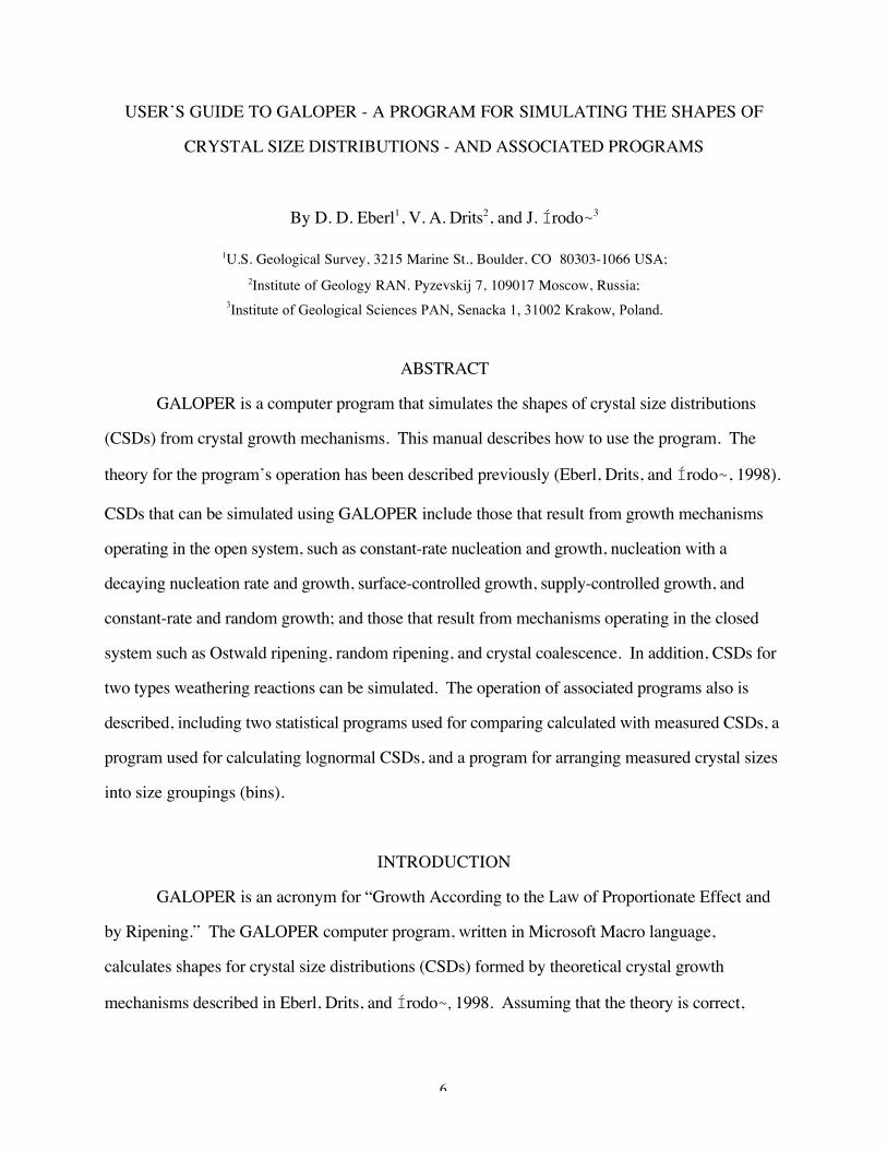
SIMULATION EXAMPLES
The first step in simulating the crystal growth mechanisms that may have produced a
measured CSD is to recognize the basic shape of the CSD. There are three basic shapes:
asymptotic (figure 3A), lognormal (figure 3B), and Ostwald ripened (figure 3C). These shapes are
produced by the crystal growth mechanism of constant-rate nucleation and growth (option 1 in the
open system), surface-controlled growth (or nucleation with a decaying nucleation rate; options 3
and 5 in the open system), and Ostwald ripening (option 1 in the closed system), respectively.

26
Next, it is necessary to recognize how the basic shape was modified by subsequent crystal growth
mechanisms. Some of these modifications, discovered through GALOPER calculations, are
presented in table 1.
A second aid in simulation is an α−β2 diagram, which is a plot of the mean of the natural
logarithms of the sizes (α) versus the variance of the natural logarithms of the sizes (β2). This
diagram will be discussed in more detail in Example 3 below. By plotting these parameters for a
CSD on this diagram, a likely reaction path for a sample can be inferred, and the CSD simulated.
Finally, chemical, geologic, isotopic and other such information about the samples can be
used as an aid. For example (Folger and others, 1997), the Ar 40/Ar 39 radiometric age of an illite
changed significantly (became younger) in a hydrothermal zone compared with a sample taken
from the same rock that was not in the reactive zone. The chemistries of the two rocks were
identical, indicating a closed system with respect to the major elements, including potassium. The
illite mean crystal thicknesses and CSD shapes also were the same in the two zones, and the rock
was not heated hot enough to lose Ar by bulk diffusion. In this case, one may suspect illite reaction
by random ripening, during which some illite crystals dissolved and then recrystallized on other
illite crystals, thereby losing Ar and becoming apparently younger. During this reaction
mechanism, a significant fraction of the illite in the hydrothermal zone could have recrystallized
without changing CSD shape or increasing the mean crystal thickness.
Below are some examples of CSD simulations for minerals from a variety of sources. The
data are in the file Examp.xls that accompanies GALOPER.
Figure 3: Three basic shapes for crystal size distributions (Kile et al., 2000).
12000960072004800240000.0
0.2
0.3
0.5
Diameter (nm)
Freq
uenc
y
ASYMPTOTICA.
432100.0
0.2
0.4
0.6
0.8
1.0
LOGNORMAL
Diameter (micrometers)
Freq
uenc
y/m
axim
um
freq
uenc
y
B.
2.01.51.00.50.00.0
0.2
0.4
0.6
0.8
1.0
Diameter/mean diameter
Freq
uenc
y/m
axim
um fr
eque
ncy
OSTWALD RIPENEDC.
27
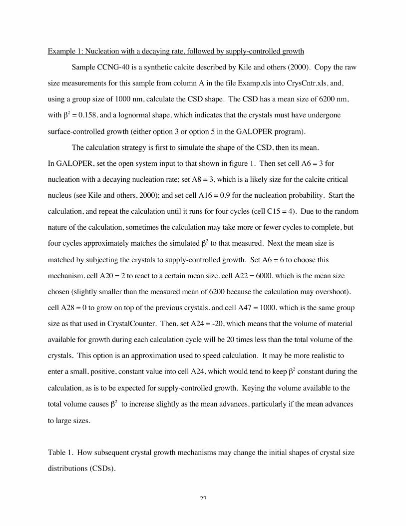
Example 1: Nucleation with a decaying rate, followed by supply-controlled growth
Sample CCNG-40 is a synthetic calcite described by Kile and others (2000). Copy the raw
size measurements for this sample from column A in the file Examp.xls into CrysCntr.xls, and,
using a group size of 1000 nm, calculate the CSD shape. The CSD has a mean size of 6200 nm,
with β2 = 0.158, and a lognormal shape, which indicates that the crystals must have undergone
surface-controlled growth (either option 3 or option 5 in the GALOPER program).
The calculation strategy is first to simulate the shape of the CSD, then its mean.
In GALOPER, set the open system input to that shown in figure 1. Then set cell A6 = 3 for
nucleation with a decaying nucleation rate; set A8 = 3, which is a likely size for the calcite critical
nucleus (see Kile and others, 2000); and set cell A16 = 0.9 for the nucleation probability. Start the
calculation, and repeat the calculation until it runs for four cycles (cell C15 = 4). Due to the random
nature of the calculation, sometimes the calculation may take more or fewer cycles to complete, but
four cycles approximately matches the simulated β2 to that measured. Next the mean size is
matched by subjecting the crystals to supply-controlled growth. Set A6 = 6 to choose this
mechanism, cell A20 = 2 to react to a certain mean size, cell A22 = 6000, which is the mean size
chosen (slightly smaller than the measured mean of 6200 because the calculation may overshoot),
cell A28 = 0 to grow on top of the previous crystals, and cell A47 = 1000, which is the same group
size as that used in CrystalCounter. Then, set A24 = -20, which means that the volume of material
available for growth during each calculation cycle will be 20 times less than the total volume of the
crystals. This option is an approximation used to speed calculation. It may be more realistic to
enter a small, positive, constant value into cell A24, which would tend to keep β2 constant during the
calculation, as is to be expected for supply-controlled growth. Keying the volume available to the
total volume causes β2 to increase slightly as the mean advances, particularly if the mean advances
to large sizes.
Table 1. How subsequent crystal growth mechanisms may change the initial shapes of crystal size
distributions (CSDs).

28
ScenarioNo.
Initial shape Subsequentgrowth
Mechanism
Final result
1 Any shape Supply-controlled or
random ripening
Preserves the initial relative shape of the CSD. β2
remains constant.
2 Asymptotic Surface-controlled
Transforms the asymptotic CSD shape into alognormal shape, sometimes leaving a pointed hat(circumflex) above the mode of the theoreticallognormal distribution.
3 Lognormal Ostwaldripening
Moves the mode of the CSD to the right of thetheoretical lognormal curve, makes the CSD moresymmetrical (β2 decreases), and finally skews theCSD to the left.
4 Lognormal McCabe’s Lawor random
growth
Shifts the mode to the left of that of the theoreticallognormal curve. Decreases β2 as the mean increases.
5 Ostwald McCabe’s Lawor random
growth
Decreases β2 as the CSD becomes narrower than theuniversal steady-state curve, and the mode shifts to theleft of the universal steady-state curve for Ostwaldripening.
29
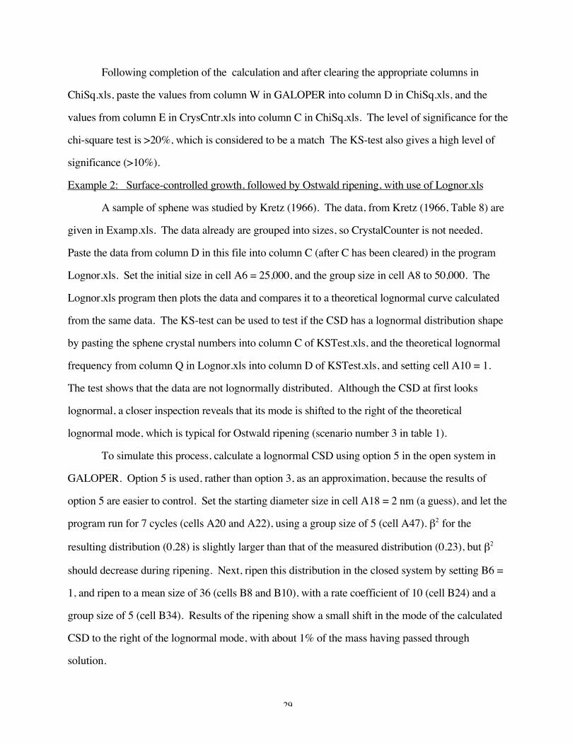
Following completion of the calculation and after clearing the appropriate columns in
ChiSq.xls, paste the values from column W in GALOPER into column D in ChiSq.xls, and the
values from column E in CrysCntr.xls into column C in ChiSq.xls. The level of significance for the
chi-square test is >20%, which is considered to be a match The KS-test also gives a high level of
significance (>10%).
Example 2: Surface-controlled growth, followed by Ostwald ripening, with use of Lognor.xls
A sample of sphene was studied by Kretz (1966). The data, from Kretz (1966, Table 8) are
given in Examp.xls. The data already are grouped into sizes, so CrystalCounter is not needed.
Paste the data from column D in this file into column C (after C has been cleared) in the program
Lognor.xls. Set the initial size in cell A6 = 25,000, and the group size in cell A8 to 50,000. The
Lognor.xls program then plots the data and compares it to a theoretical lognormal curve calculated
from the same data. The KS-test can be used to test if the CSD has a lognormal distribution shape
by pasting the sphene crystal numbers into column C of KSTest.xls, and the theoretical lognormal
frequency from column Q in Lognor.xls into column D of KSTest.xls, and setting cell A10 = 1.
The test shows that the data are not lognormally distributed. Although the CSD at first looks
lognormal, a closer inspection reveals that its mode is shifted to the right of the theoretical
lognormal mode, which is typical for Ostwald ripening (scenario number 3 in table 1).
To simulate this process, calculate a lognormal CSD using option 5 in the open system in
GALOPER. Option 5 is used, rather than option 3, as an approximation, because the results of
option 5 are easier to control. Set the starting diameter size in cell A18 = 2 nm (a guess), and let the
program run for 7 cycles (cells A20 and A22), using a group size of 5 (cell A47). β2 for the
resulting distribution (0.28) is slightly larger than that of the measured distribution (0.23), but β2
should decrease during ripening. Next, ripen this distribution in the closed system by setting B6 =
1, and ripen to a mean size of 36 (cells B8 and B10), with a rate coefficient of 10 (cell B24) and a
group size of 5 (cell B34). Results of the ripening show a small shift in the mode of the calculated
CSD to the right of the lognormal mode, with about 1% of the mass having passed through
solution.

30
The calculation can be continued by using supply-controlled growth to preserve the shape
and β2 of the CSD as the mean size increases. This can be done by pasting the ripened CSD into
the open system (set cell A62 = 1 and start the calculation); then start supply-controlled growth to a
mean of 212,000 nm. However, because it is known that β2 will remain constant during this
simulation, it is easier to model this last mechanism rather than to simulate it. The last mechanism
can be modeled by multiplying the distribution by a constant (proportionate growth option in cell
A69). The constant to be used is the sample mean divided by the ripened mean, or 21,2487 ÷ 36 =
5,902. To carry out this procedure, first paste the ripened system into the open system (set cell A62
= 1 and start). Next set cells A6 = 5, A28 = 0, A47 = 25,000, A62 = 0, and A69 = 5,902. Run the
calculation for one cycle (done automatically if cells A20 and A22 were not changed from the
previous calculation). By combining groups in the GALOPER calculation using a separate
worksheet, so that the GALOPER size categories match those given by Kretz (1966), the KS-test
indicates that the calculated and measured distributions are the same at the 5-10 % level of
significance. The calculation shows that even a very small amount of ripening can be detected in the
CSD shape.
Example 3: A second nucleation, and use of an α−β2 diagram
An an α−β2 diagram is shown in figure 4, on which have been plotted parameters for a
hydrothermal illite collected from a bore hole in Red Mountain, Lake County, Colorado. This
diagram was constructed using GALOPER calculations; the crystal thickness distribution for the
sample was measured by X-ray diffraction (XRD) using the MudMaster computer program (Eberl
and others, 1996) and the PVP-10 intercalation technique to remove the effects of swelling from
XRD peak broadening (Eberl, Nüesch, and others, 1998). Curve A-B is calculated for the evolution
of β2 with α for constant-rate nucleation and growth (option 1 in the open system), starting with a
2-nm thick critical nucleus (the thickness of an elementary illite particle). The numbered pluses on
this curve are the number of nucleation cycles. The shapes of the CSDs formed along this curve
are expected to be asymptotic. Curve A-C was calculated for surface-controlled growth (option 5)
with a 2-nm thick starting diameter. The ticks on this curve also refer to the number of calculation
31
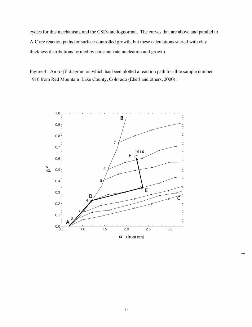
cycles for this mechanism, and the CSDs are lognormal. The curves that are above and parallel to
A-C are reaction paths for surface-controlled growth, but these calculations started with clay
thickness distributions formed by constant-rate nucleation and growth.
Figure 4. An α−β2 diagram on which has been plotted a reaction path for illite sample number1916 from Red Mountain, Lake County, Colorado (Eberl and others, 2000).
3.02.52.01.51.00.50.50.0
0.1
0.2
0.3
0.4
0.5
0.6
0.7
0.8
0.9
1.0
α
β
2
3
4
5
6
7
E
F1916
A
D
B
C
(from nm)
2

32
Figure 5. Simulated and measured crystallite thickness distribution for illite sample number 1916(Eberl and others, 2000).
The α and β2 values for sample 1916 are plotted in figure 4, and the sample’s measured
CSD is given in figure 5 (open circles). The CSD would appear to be lognormal, except that it is
bimodal and has a second peak at 2 nm, as though there was a second nucleation event. The
thickness distribution, which is given in the file Examp.xls, was modeled by trial and error. The
reaction path through the α - β2 diagram that best simulates the CSD shape is: (1) path A-D (figure
4) with nucleation and growth for 4 cycles (option 1 with 250 nuclei per cycle), followed by (2)
path D-E with surface-controlled growth without nucleation for 3 cycles (option 5), followed by (3)
path E-F with a second nucleation event that nucleated 125 additional 2-nm thick crystals. When
this exact path is followed, the simulated and measured distributions are significantly correlated
(>10% by the KS-test).
504030201000.00
0.05
0.10
0.15
SimulatedMeasured
Thickness (nm)
Freq
uenc
y
33
The last stage in the simulation, during which new nuclei were added to the lognormal-like
CSD formed along path A-D-E, was accomplished by setting cell A6 = 1, cell A14 = 1, and cell
A28 = 0, then starting the program. This calculation randomizes crystal sizes in the column in
which they are stored to insure that they are not sorted with respect to size. Next, by setting cell
A12 = 125 and cell A14 = 0, 125 new 2-nm thick crystals are added to the distribution, resulting in
the calculated CSD shown in figure 5. In the simulation, the secondary nuclei replace crystals
already stored in the program, which is a calculation trick. Of course, the additional nuclei in nature
would be added to crystals already present, without replacing them. But this trick was used
because the program has room for only 1001 crystals. The results are nearly equivalent if the
preexisting crystals are replaced randomly with respect to size.
REFERENCES
Blum, A. E., and Eberl, D. D., 1992, Determination of clay particle thickness and morphology using
Scanning Force Microscopy, in Kharaka, Y. K., and Maest, A. S., eds., Water-rock
interaction, volume 1, Low temperature environments: Amsterdam, A. A. Balkema, p. 133-
136.
Drits, V., Eberl, D. D., and Srodon, J., 1998, XRD measurement of mean thickness, thickness
distribution and strain for illite and illite/smectite crystallites by the Bertaut-Warren-
Averbach technique: Clays & Clay Minerals, v. 46, p. 38-50.
Eberl, D. D., Kile, D. E., and Bove, D. J., 2000, The shapes of crystal size distributions for minerals
are reaction path dependent: calcite and illite examples: Geological Society of America 2000
Annual Meeting, Abstracts with Programs, v. 32, p. A-320.
Eberl, D. D., Drits, V., Írodo~, J., and Nüesch, R., 1996, MudMaster: A program for calculating
crystallite size distributions and strain from the shapes of X-ray diffraction peaks: U.S.
Geological Survey Open-File Report 96-171, 46 p.
Eberl, D. D., Drits, V. A., and Írodo~, J., 1998, Deducing growth mechanisms for minerals from
the shapes of crystal size distributions: American Journal of Science, v. 298, p. 499-533.

34
Eberl, D. D., Nüesch, R., Sucha, V., and Tsipursky, S., 1998, Measurement of fundamental illite
particle thicknesses by X-ray diffraction using PVP-10 intercalation: Clays & Clay
Minerals, v. 46, p. 89-97.
Folger, H. A., Eberl, D. D., Hofstra. A. H., and Snee, L. W., 1997, Illite crystallinity – a key to
understanding 40Ar/39Ar dates from gold deposits in the Jerritt Canyon district, Nevada:
Geological Society of America 1997 Annual Meeting, Abstracts with Programs, v. 29, p.
A207.
Kile, D. E., and Eberl, D. D., 1999, Crystal-growth in miarolitic cavities in the Lake George ring
complex and vicinity, Colorado: American Mineralogist, v. 84, p. 718-724.
Kile, D. E., Eberl, D. D., Hoch, A. R., and Reddy, M. M., 2000, An assessment of calcite crystal
growth mechanisms based on crystal size distributions: Geochimica et Cosmochimica Acta,
v. 64, p. 2937-2950.
Kretz, R., 1966, Grain-size distribution for certain metamorphic minerals in relation to nucleation
and growth: Journal of Geology, v. 74, p. 147-173.
Írodo~, J., Eberl, D. D., and Drits, V. A., 2000, Evolution of fundamental-particle size during
illitization of smectite and implications for reaction mechanism: Clays & Clay Minerals, v.
48, p. 446-458.
35
APPENDIX 1: SUMMARY OF INPUTS FOR THE OPEN SYSTEM.
Input Cell Value Comments
Open system option A6 1 to 7 Choose the crystal growth mechanism. To grow ontop of previously formed crystals, set A28 = 0.
Size of critical nucleus A8 >0 For options 1-4, this is the size of the crystals thatappear during nucleation. Usually this value this is aguess that is several unit cell sizes.
Particles to nucleateper cycle
A10 1 to 1001 Input for options 1 & 2. The number of nucleationcycles = A30/A10.
Nucleate on previousCSD?
A12 0 = no; or givenumber of new
nuclei
Cell A6 must = 1. These nuclei replace crystalsformed previously, which should not be sorted withrespect to size. Therefore, the stored crystal sizesshould be randomized first (see cell A14).
Randomize crystalsizes?
A14 0 to 2 Stored crystal sizes should be randomized beforecalculating a second nucleation event (cell A12) inorder to randomly replace previously formedcrystals.
Probability for criticalnucleus formation
A16 A fractionranging from
>0 to <1.
For option 3, the probability that a crystal willnucleate during each calculation cycle. Nucleationceases when a maximum of 1001 crystals havenucleated.
Starting diameter A18 >0 For options 5 – 7, the starting diameter for all of thecrystals prior to growth. Active if A28 = 1.
Criteria for growth A20 1 or 2 For options 5 –7, entering “1” will grow todesignated mean size, “2” to number of cycles.

36
Appendix 1 (continued)
Total number of cyclesor mean
A22 >0 For options 5-7, enter number of calculations cycles(A20 = 1) or mean size (A20 = 2) to be attainedduring calculation.
Volume to be addedper cycle
A24 Positive ornegativenumber
For options 2, 4 and 6, the volume that is added tothe crystals during each growth cycle. A negativenumber adds a fraction of the current total volume(e.g. –10 adds 0.1 x total volume for each calculationcycle; -100 adds .01 x total volume, etc.).
Reduce volumeavailable by growthvolume
A26 0, 1, or 2 For options 2, 4 and 6, entering “1” or “2”reduces the volume in cell A24 by the volume usedduring growth cycles.
Clear old data? A28 0 = no;1 = yes
If A28 = 1, crystal growth starts fresh; if = 0, growthis on top of previously formed crystals. Set to 0 forsupply-controlled growth (options 2,4, and 6).
Total number ofcrystals
A30 1 to 1001 Number of crystals that nucleate and/or grow duringthe calculation.
Epsilon variation A32&
A33
Range ofvalues, usually0 to 1.
The range allowed for the random number used inthe Law of Proportionate Effect (equation 1).
Crystal shape A35 1 or 2 Calculates either spheres (1) or cubes (2). Relativeanswers will not change; only absolute volumeschange.
Mineral density A37 Give density, ing/cm3
Used for calculating the specific surface area of amineral.
Appendix 1 (continued)Rate coefficient A39 Generally use 1 Input can be used to tweak the calculation so that it
approaches a desired mean. Best to leave at 1, orchange very slightly.

37
approaches a desired mean. Best to leave at 1, orchange very slightly.
Collect openfrequency?
A41 0 = no; or giveiterations
Open system can be iterated several times so that thefrequency distribution can be plotted moreaccurately, using more than 1001 crystals. Thesefrequencies are stored in column AK. For use onlywith options 1, 3, 5, and 7. Data can not be re-plotted.
Update screen A43 1 = yes Set at “1” to watch the calculation happen.Otherwise, screen updates automatically at end ofcalculation.
Give plot? A45 0, 1, or 2 Calculation can be terminated by pressing escapekey, and the results plotted by setting this cell to 2.
Group size A47 integer Bin size for the calculation. Results can be replottedwith different size by changing A45 and this cell.
Clear chart? A49 1 = yes Keep former chart to compare calculations.
Do not count particlesless than:
A51 Positivenumber or zero
Plotting and results will ignore crystals smaller thanthis value.
How to collect data A53 0, -1, 1 Should data be collected into bins starting fromcenter, beginning, or end of group size? Always use0.
Continue with closedsystem?
A56 1 = yes Calculation will continue with closed-systemcalculation after open-system calculation iscomplete.

38
Appendix 1 (continued)Iterate closed system? A58 0 = no; or enter
number ofiterations
Open and closed systems are iterated to create lessnoisy CSDs for long ripenings.
Collect ripenedparticles?
A60 1 = yes Crystals that remain from each ripening iteration arecollected in column DB. They can be pasted intoopen system using cell B41.
Paste ripened intoopen system?
A62 1 = yes Crystals from closed system are pasted into opensystem. Use cell B41 to paste crystals collectedduring ripening iterations into open system.
LPE weathering? A65 1 = yes Use option 5; set epsilon to a smaller variation (A33)to induce supply-controlled weathering.
McCabe’s Law growth A67 0 = no; or givesize increase
Constant linear amount added to each crystal. Useoption 5 (cell A6) and save old data (set A28 = 0).
Proportionate growth A69 0 = no; or givemultiplier
Each crystal size is multiplied by a constant. Useoption 5 (cell A6) and save old data (set A28 = 0).
39
APPENDIX 2: SUMMARY OF INPUTS FOR CLOSED SYSTEMInput Cell Value Comments
Ripening options B6 1 to 4 Choose ripening mechanism.
Ripen to number ofcycles, mean, fraction ornumber of particles
B8 1 to 4 For option 1, one can choose to ripen to a certain numberof cycles (1), to a mean size (2), to a fraction of materialpassing through solution (3), or to a number of crystalsremaining in the system (4).
Ripen to this number B10 Number orfraction
For option 1, choose how far to ripen, given the entry incell B8.
Diffusion or surface-controlled ripening?
B12 1 or 2 For options 1, 2, or 3, choose ripening mechanism.Diffusion-controlled ripening seems to be the commonone (enter 1).
Size of critical diameter B14 Enter size For options 2 and 3, the critical radius for ripening (seeequation 3) will be fixed at this value/2.
Number of cycles B16 Enternumber
For option 3, the number of ripening cycles usingequation 3 and the fixed critical radius (B14).
Probability for randomdissolution
B18 Fractionfrom 0-1
For option 4, probability that a crystal will dissolvewithout respect to size (random ripening).
Dissolve only < this size B20 Enter size For option 4, only crystals less than this size have aprobability to dissolve.
Clear old data? B22 1 = yes Set to “0” to ripen previously ripened distribution.
Rate coefficient B24 Positivenumber
Increase number to increase ripening rate.
40
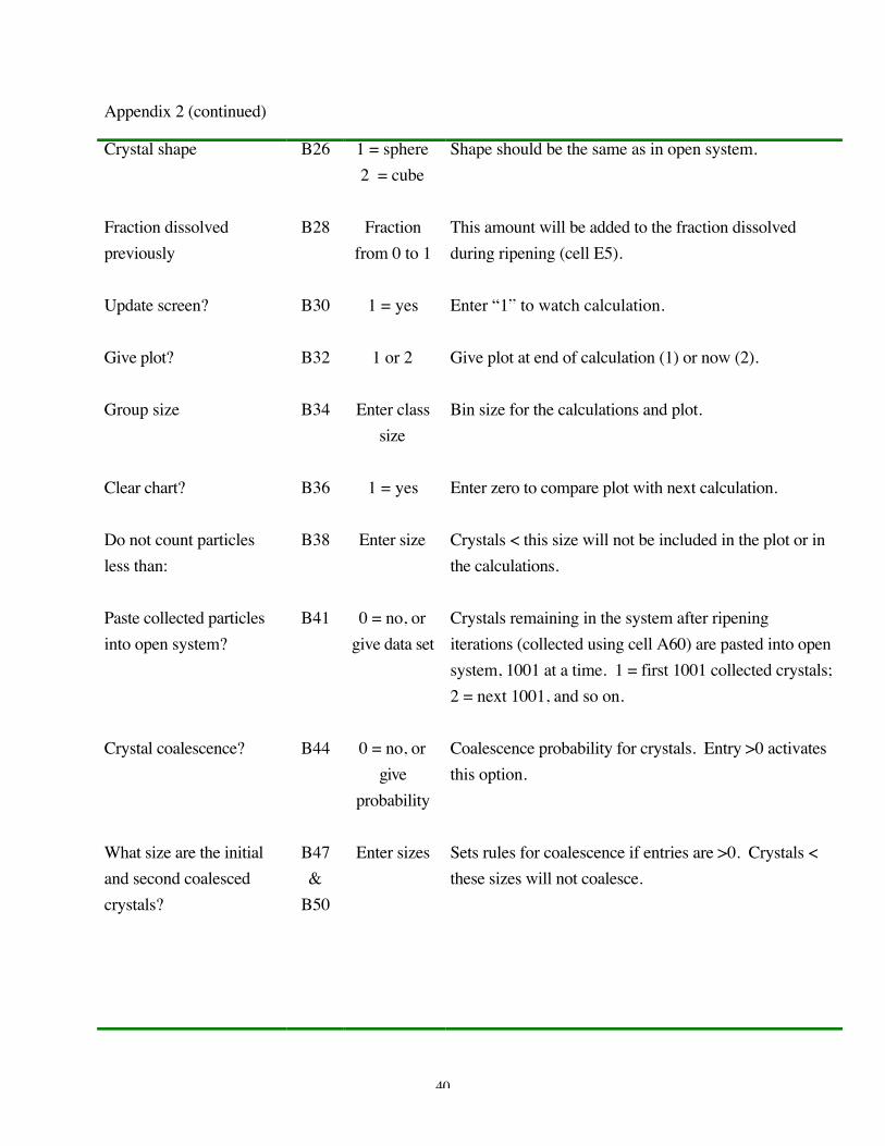
Appendix 2 (continued)
Crystal shape B26 1 = sphere2 = cube
Shape should be the same as in open system.
Fraction dissolvedpreviously
B28 Fractionfrom 0 to 1
This amount will be added to the fraction dissolvedduring ripening (cell E5).
Update screen? B30 1 = yes Enter “1” to watch calculation.
Give plot? B32 1 or 2 Give plot at end of calculation (1) or now (2).
Group size B34 Enter classsize
Bin size for the calculations and plot.
Clear chart? B36 1 = yes Enter zero to compare plot with next calculation.
Do not count particlesless than:
B38 Enter size Crystals < this size will not be included in the plot or inthe calculations.
Paste collected particlesinto open system?
B41 0 = no, orgive data set
Crystals remaining in the system after ripeningiterations (collected using cell A60) are pasted into opensystem, 1001 at a time. 1 = first 1001 collected crystals;2 = next 1001, and so on.
Crystal coalescence? B44 0 = no, orgive
probability
Coalescence probability for crystals. Entry >0 activatesthis option.
What size are the initialand second coalescedcrystals?
B47&
B50
Enter sizes Sets rules for coalescence if entries are >0. Crystals <these sizes will not coalesce.
41
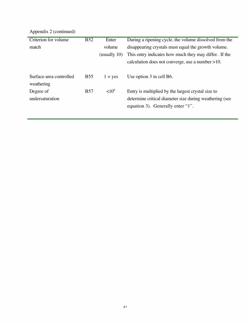
Appendix 2 (continued)Criterion for volumematch
B52 Entervolume
(usually 10)
During a ripening cycle, the volume dissolved from thedisappearing crystals must equal the growth volume.This entry indicates how much they may differ. If thecalculation does not converge, use a number >10.
Surface-area controlledweathering
B55 1 = yes Use option 3 in cell B6.
Degree ofundersaturation
B57 <106 Entry is multiplied by the largest crystal size todetermine critical diameter size during weathering (seeequation 3). Generally enter “1”.

42
APPENDIX 3: SUMMARY OF RESULTS FOR OPEN SYSTEMResult Cell Comments
Mean diameter C3 X = Xf X( )∑ , where f(X) is the frequency of diameter X.
Alpha C5 α = ln X( )∑ f X( ) .
Beta2 C7β2 = lnX − α( )∑ 2f X( ) .
Number of particles C9 Number of crystals in the system.
Number of particlesnot counted
C11 Crystal sizes that fall outside of the end of the calculateddistribution. To include these crystals, replot (set cell A45 = 2)with larger group size (A47).
Diameter of largestparticle
C13 Size of largest crystal in distribution.
Total number ofcycles
C15 Total number of cycles in the calculation.
Total surface area C17 Total surface area for spherical or cubic crystals (set shape in cellA35).
Total volume C19 Total volume for spherical or cubic crystals (set shape in cell A35).
Specific surface area C21 Uses density in cell A37 to calculate specific surface area in squaremeters per gram.

43
APPENDIX 4: SUMMARY OF RESULTS FOR CLOSED SYSTEMResult Cell Comments
Mean diameter D3 X = Xf X( )∑ , where f(X) is the frequency of diameter X.
Alpha D5 α = ln X( )∑ f X( ) .
Beta2 D7β2 = lnX − α( )∑ 2f X( ) .
Number of particles D9 Number of crystals in the system.
Number of particlesnot counted
D11 Crystals that fall outside of the end of the calculateddistribution. To include these crystals, replot (set cell B32 = 2)with larger group size (B34).
Diameter of largestparticle
D13 Size of largest crystal in distribution.
Diameter of smallestparticle
D15 Size of smallest crystal in distribution.
Number of cycles D17 Number of cycles in the calculation.
Number of iterations D19 Number of times ripening calculation was repeated starting withopen system (see cell A58).
Units of diameterdissolved
E3 Sum of the length of crystals dissolved during previouscalculation cycle.
Fraction of corevolume dissolved
E5 Fraction of original material that has passed through solutiononce during the ripening process.
44
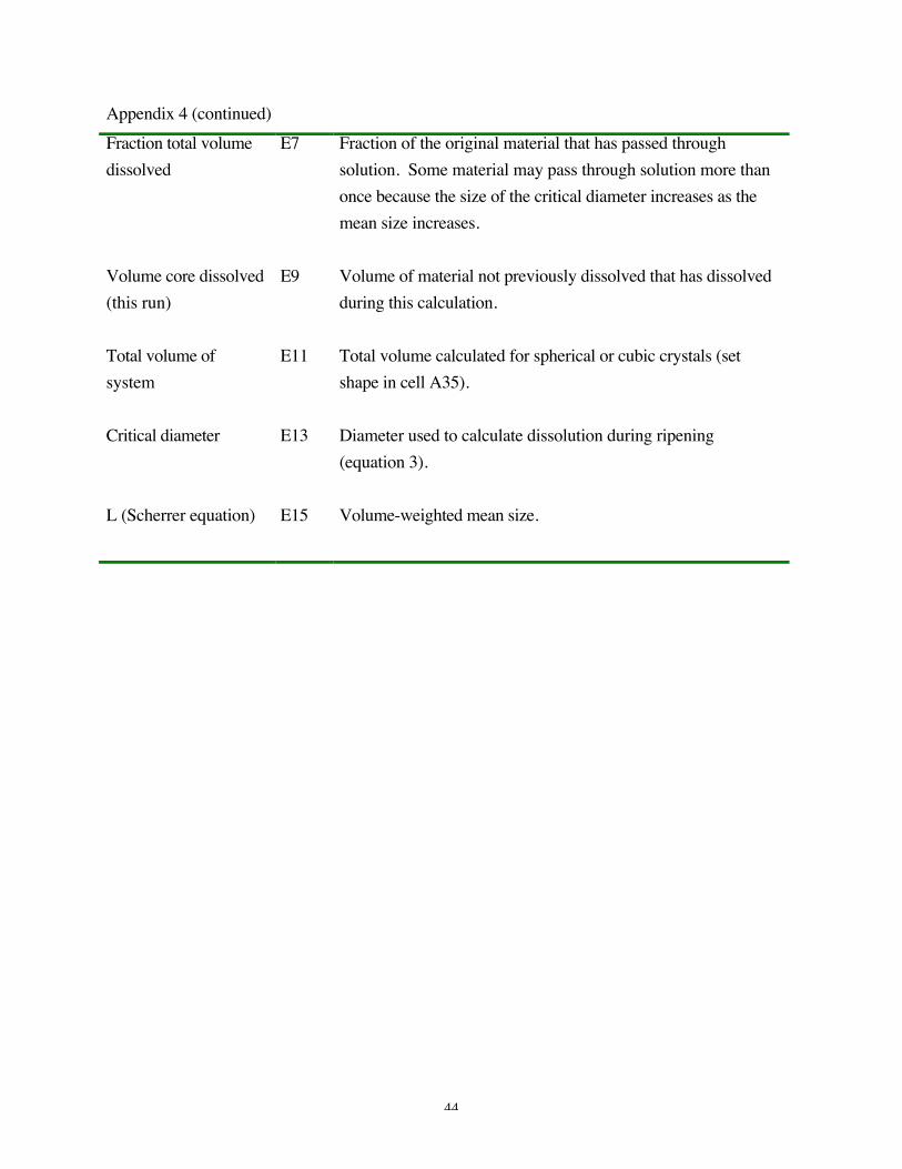
Appendix 4 (continued)Fraction total volumedissolved
E7 Fraction of the original material that has passed throughsolution. Some material may pass through solution more thanonce because the size of the critical diameter increases as themean size increases.
Volume core dissolved(this run)
E9 Volume of material not previously dissolved that has dissolvedduring this calculation.
Total volume ofsystem
E11 Total volume calculated for spherical or cubic crystals (setshape in cell A35).
Critical diameter E13 Diameter used to calculate dissolution during ripening(equation 3).
L (Scherrer equation) E15 Volume-weighted mean size.
Top Related