


Languages
Pages
Legal

USE OF PRECISION AGRICULTURAL-LANDSCAPE MODELING SYSTEM (PALMS) FOR ESTIMATING
THE EFFECTS OF CULTURAL PRACTICES ON INFILTRATION, RUNOFF AND EROSION
MSc Thesis by Carlos Álvarez Acosta
December 2009
1


Use of Precision Agricultural-Landscape Modeling System (PALMS) for estimating the effects of cultural practices on
infiltration, runoff and erosion
By
Carlos Álvarez Acosta
Master thesis Land Degradation and Development Group submitted in partial fulfillment of the
degree of Master of Science in International Land and Water Management at Wageningen
University, the Netherlands
Study program:
MSc International Land and Water Management (MIL)
Student registration number:
830503‐013‐080
LDD 80336
Supervisor(s):
Dr. Ir. Leo Stroosnijder
Dr. Robert J. Lascano
Examinator:
Dr.ir. Leo Stroosnijder
Date: December 2009
Wageningen University, Land Degradation and Development Group.
United States Department of Agriculture. Agriculture Research Service. Cropping System Research
Laboratory. Lubbock, Texas.

PREFACE
All the good things come to an end, and definitely this experience has been something very positive for me. I have learned many things not only related to the thesis itself, but also about agriculture and about the culture in the USA, which is not far from the European, but still is not the same. This experience has enriched me as a person and as a professional, and helped to open my mind and see different ways of thinking which I am sure was also part of the intended outcomes of doing a thesis abroad.
This research wouldn’t have been possible without the help of many people that has supported me all this time, so I want to thank them all for their help.
Now that I know that I’m not forgetting anyone, I would like to thank the people in the Cropping system research Laboratory, in Lubbock, Texas, that were always willing to answer my questions (Randall, Vinicius, Wade and a long etc). Christine from the University of Wisconsin‐Madison was amazingly helpful and I really appreciate her speed at answering my doubts about PALMS.
Special thanks must be given to Robert as he always treated me very kindly, he had always time for me and worked hard so I could finish it on time. Robert and Leo directed me wisely and I have never had better supervisors, thank you very much. .Jill and JD deserve a special mention as they hosted me at their home. I can’t think of a better place to stay, nor anyone better to show me the “surroundings”. I had a great time with them and their funny Shasha and Baylea.
Last and therefore, the most important, Esther. Being so far away from you have been tough, but every time I needed help you were and will always be there.
Carlos Álvarez Acosta
Lubbock, 16 November 2009

ABSTRACT Agriculture worldwide and particularly in the United States, is under increasing pressure to reduce the negative environmental consequences of its management and cultural practices, but at the same time, enhance its production. This research was conducted in a 63.8‐ha field near Lamesa, Texas, USA. Our objective was to evaluate water harvested from rain and the reduction of soil loss under semiarid conditions, by comparing planting dryland crops in a circular pattern instead of the traditional linear rows. Further, we also evaluated the effect of tillage operations in circular versus linear rows. The Precision Agricultural‐Landscape Modeling System (PALMS) was used to calculate infiltration, runoff and erosion in the field comparing linear versus circular rows at a landscape scale. Textural analysis and soil hydraulic parameters (Ksat, water retention curve) were measured across the field and used as input and also to calibrate the model for the study area. The study field has an average slope of 0.33 % and thus erosion calculations showed that soil erosion was minimal with only a slight redistribution of soil within the field boundary conditions. PALMS calculations also showed that planting a dryland crop, such as sorghum (Shorgum bicolor L.) in a circular pattern and not in the traditional linear row, did not modify the annual infiltration (254 mm yr‐1), runoff (22,000 m3 ha‐1 yr‐1) and erosion (1.2 Mg ha‐1 yr‐1). Although PALMS yielded reasonable estimates, further calibration is needed in order to further verify calculations of all model outputs.

TABLE OF CONTENT
1. INTRODUCTION 8
1.1 NEED OF A MORE EFFICIENT CROP MANAGEMENT 8 1.2 OBJECTIVES 9
2. MATERIALS AND METHODS 10
2.1 STUDY AREA 10 2.2 PALMSMODEL DESCRIPTION
GRICULTURAL‐LANDSCAPE MODELING SYSTEM (PALMS) 11
CISIO A
14
11 2.2.1 PRE N
2.2.2 I PUT DATA 16
N
2.2.3 OUTPUT DATA 2.2.4 MAIN EROSION PROCESSES IN PALMS 16 2.3 L TORY WORK 19 ABORA
XTURAL ANALYSIS
SAT) 21 2.3.1 TE2.3.2 LABORATORY PERMEAMETER PROCEDURE (K2.3.3 WATER RETENTION CURVE DETERMINATION 25
19
2.4 MODEL PERFORMANCE EVALUATION 27
3. RESULTS AND DISCUSSION 29
3.1 29 L TORY RESULTS 29
ABORA
3.1.1 EXTURES (PIPPETE METHOD) CONDUCTIVITY (KSAT) 32
T3.1.2 SATURATED HYDRAULIC 3.1.3 SOIL WATER RETENTION 33 3.2 ROSETTA SIMULATION 35 3.3 MODEL CALIBRATION 36 3.4 MODEL VALIDATION 38 3.4.1 INFILTRATION 38 3.4.2 RUNOFF 40 3.4.3 EROSION 42
4. CONCLUSIONS AND RECOMMENDATION 45
5. REFERENCES 46
6. APPENDIX I

8
1. Introduction
1.1 Need of a more efficient crop management
Worldwide agriculture and in particular the United States, is under increasing pressure to enhance agricultural production and, at the same time, reduce the negative environmental consequences from its practices (Morgan, 2003). Water supply represents the greatest limitation to production under rain‐fed conditions (Morrow and Krieg, 1990); therefore, it is necessary to “harvest” the maximum amount of rain possible, in order to obtain maximum crop yield under dryland conditions.
Soil‐erosion problems were noted in the United States during Colonial times. In the years that followed, advancements in agricultural practices frequently resulted in high erosion rates (Toy, 2002). Due to the erosion problems and the scarcity of water in the North‐West Texas (USA), crop yields are being reduced. The 'rule of thumb' is that about 50% of rainfall is lost due the effect of water runoff (R.J. Lascano, personal communication). These problems highlight the need to find solutions that can reduce the effect of the weathering process and help water infiltrate as much as possible to increase water availability for the crop. Further, in the Texas High Plains the decrease of irrigation water from the Ogallala aquifer, highlights the importance of dryland production (Lascano, 2000). Every year close to one million ha are planted with cotton and the current ratio of irrigated versus dryland production is 1 to 1, i.e., 50% of the area is at the mercy of rain received during the growing season and the amount of dryland production will continue to increase. To sustain economic stability due to the reduction of agricultural production, we need methods to increase water from rainfall, i.e., reduce water runoff.
To achieve a higher production of crop yield and reduce negative environmental impacts, there is a need to identify where the problem is and its importance in terms of how it affects crop production. According to (Toy, 2002) there are five reasons for erosion measurements, but this project is mainly focusing on one of them, i.e., the evaluation of technology to calculate erosion using a simulation model. For this purpose we selected and used the Precision Agricultural‐Landscape Modeling System (PALMS).
There is a need to understand the processes involved in the management of agricultural fields in production, to achieve an increase in crop yield without damaging the environment. The main objective is to increase rain‐water infiltration and minimize a crop yield reduction in areas where there is a transition from irrigation to dryland production. This is the likely scenario in the Texas High Plains where the decline of irrigation water is forcing producers to abandon irrigation‐wells and adopt practices of dryland production.
According to (Stroosnijder, 2005), erosion‐prediction technologies will always be related to measurements and the other way around. Measurements alone would provide data difficult to extrapolate in time and space, meaning that erosion in large fields would not be known without prediction technologies, but also that predictions need measurements to work.

9
1.2 Objectives
The aim of this study was to evaluate the effects of planting a dryland crop, Sorghum (Sorghum Bicolor L.), in circular instead of linear rows. Our hypothesis was that planting dryland crops under semiarid conditions in a circular pattern would increase the amount of water available for the plant and thus yield by increasing water infiltration of rain and reducing soil erosion.
The following sub‐objectives were taken into account:
1. The modification of the processes of infiltration, runoff, and erosion when the planting pattern was changed from the traditional linear to circular rows.
2. Test the use of the Precision Agricultural‐Landscape Modeling System (PALMS) to calculate the water balance, runoff and erosion algorithms for the semiarid climate conditions in the study area.
2. Materials and Methods
2.1 Study Area
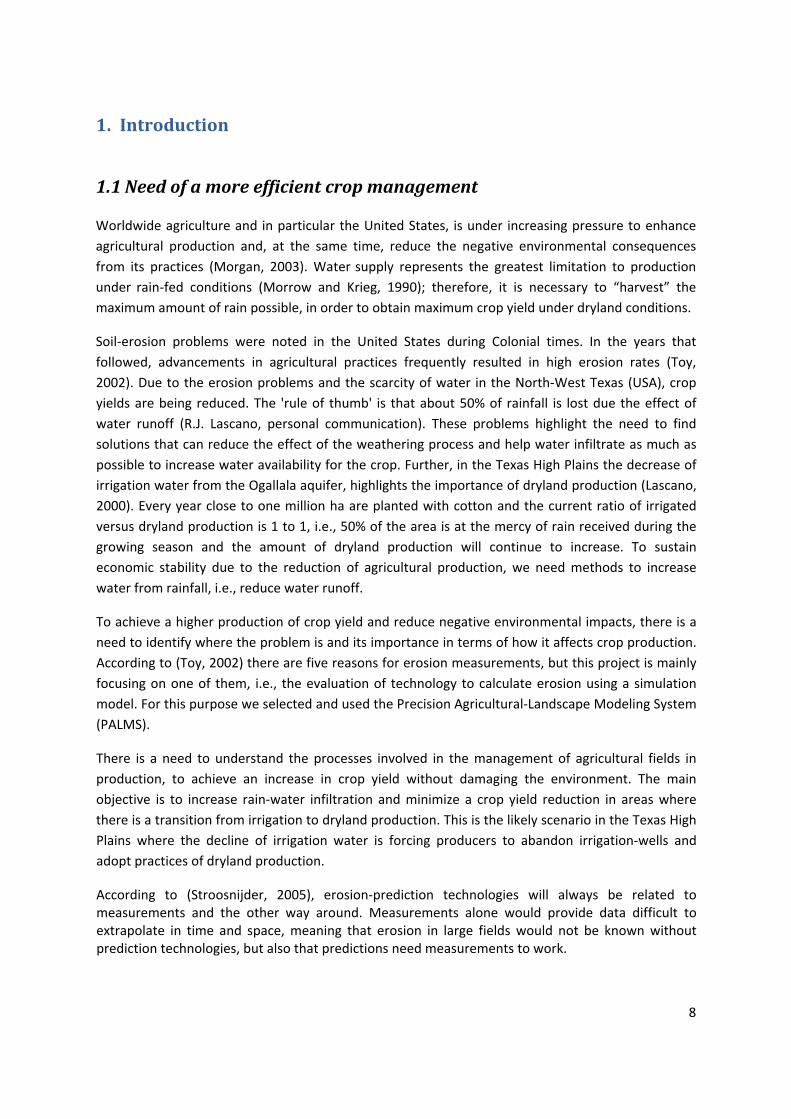
The study field is situated in the region known as Llano Estacado, near Lamesa, which is a small town, population of close to 104, located in Dawson County, North West Texas, USA (see Fig. 1). Its coordinates are 32° 32’ 7.4’’ N; 101° 46’ 8.24’’ W; and, elevation of 833 m above sea level. The study field has an area of 63.8 ha and an average slope of 0.33 %. In 2008, the field was planted with dryland sorghum (Sorghum Bicolor L.). The field is owned and operated by a farmer that has a cooperative agreement with the Texas AgriLife Research (R.J. Lascano, personal communication). In this region, about half the cultivated land is irrigated from an underground aquifer, called the Ogallala, which is classified, as non‐rechargeable. Therefore it is important to use the scarce resource of water as efficiently as possible by “harvesting” more rain. This research attempts to identify a pattern of planting dryland crops in circles and not using the traditional linear rows, to reduce water erosion and increase rainfall water harvesting. The idea is that by planting crops in circles will minimize soil erosion, with the long‐term benefit of increasing the amount of water available for plants, and the reduction of sorghum yield due to the effect of the weathering processes will also be minimized.
10
Figure 1. Location of study field in Texas, USA.
Lamesa
800 m
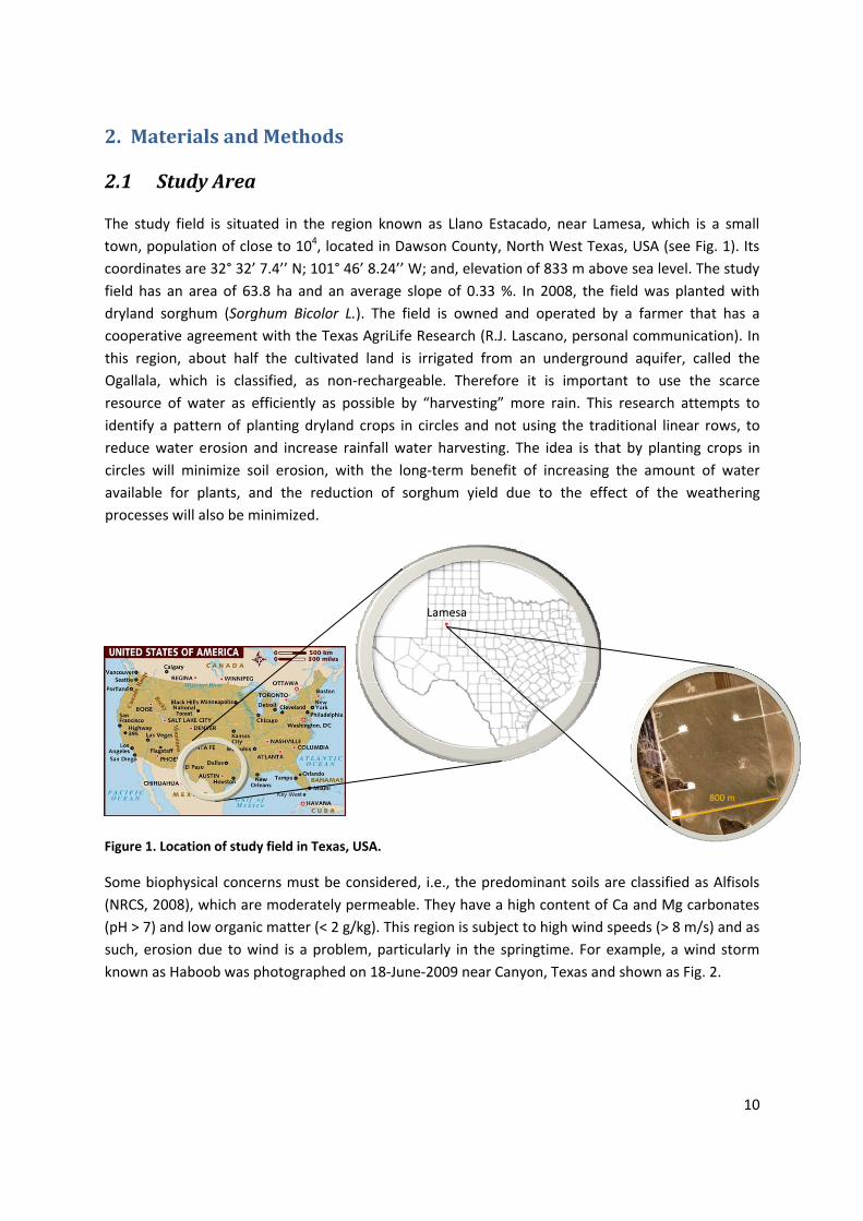
Some biophysical concerns must be considered, i.e., the predominant soils are classified as Alfisols (NRCS, 2008), which are moderately permeable. They have a high content of Ca and Mg carbonates (pH > 7) and low organic matter (< 2 g/kg). This region is subject to high wind speeds (> 8 m/s) and as such, erosion due to wind is a problem, particularly in the springtime. For example, a wind storm known as Haboob was photographed on 18‐June‐2009 near Canyon, Texas and shown as Fig. 2.
Figure 2. A windstorm known as Haboob on 18‐June‐2009 near Canyon, Texas (John Stout, personal communication).
Rainfall events in this region are categorized as of short duration but high intensity, e.g., 20 mm of rain in 15 min, and as such water runoff is high (R. J. Lascano, personal communication). The mean annual precipitation in the study area is 483 mm with a mean annual air temperature of 16 °C (NRCS, 2008).
According to (NRCS, 2008) the following horizons are typical for the soils of the study area:
Ap = Darker surface horizon or topsoil, which has been plowed and disturbed. Sometimes there are two colors in this horizon named Ap1 and Ap2.
Bt = Subsoil with illuvial clay. Some difference in color and/or structure can be found in this horizon so that in some cases three sub‐horizons (Bt1, Bt2 and Bt3) can be identified.
Btk = Subsoil with translocation of clay but also presence of calcium carbonates (CaCO3, < 50 %). This can be divided into Btk1 and Btk2 if any differences in structure and/or color are present.
Bkk = Subsoil with abundant blocks of calcium carbonates (CaCO3, maximum of 60 %).
2.2 PALMS model description
2.2.1 Precision agriculturalLandscape Modeling System (PALMS)
The Precision Agricultural‐Landscape Modeling System (PALMS) is a computer simulation model used in farm management that works in a quasi‐three‐dimensional system that was developed by Dr. John Norman and co‐workers at the University of Wisconsin, Madison. It is still under
11
12
development, but was first developed as a primary component of a precision agriculture decision support system under NASA’s Regional Earth Science Applications Center (RESAC) program. The Precision Agricultural‐Landscape modeling system simulates physical and biophysical processes at the level of physical realism and spatio‐temporal detail, that works as a support in the decision‐making to manage not only the cropping, tillage and fertilizer but also the economics of a farm enterprise (Morgan, 2003).
Some models used by farmers are designed to maximize crop yield, but ignore the long‐term impact of several processes, such as maintenance of soil organic matter, non‐point source pollution, nutrient replenishment, etc. (Molling, 2005). The model PALMS is capable of simulating different management scenarios while taking into account the long‐term impact of environmental factors. The model PALMS has been shown to be a good erosion predictor model compared with the WEPP (Water Erosion Prediction Project), and is capable of quantifying spatial and temporal distributions of evapotranspiration, photosynthesis, infiltration, drainage, crop growth and yield, etc. in topographically complex landscapes (Bonilla et al., 2007). Further verifications have been done and according to (Bonilla et al., 2008), PALMS calculations are more accurate in large events, which is desirable, as the model is intended to be used for farm‐management environmental decisions at a landscape scale.
Simulations with the PALMS model require minimal input information to be executed. These inputs include the spatial distribution of key soil properties, such as depth of the A horizon, texture of the A and B horizons, and depth to the root‐limiting horizons (Zhu, 2004). It is structured on a three‐dimensional grid in such a way that soil‐water interactions are linked on the meso‐ and micro‐scale. It requires a three‐dimensional soil map, on a 5 to 20‐m grid, with the topography.
There are several models capable of calculating erosion, but according to (Molling, 2005) no single existing model or modeling approach, other than PALMS, is capable of representing all of the following characteristics: physically based representation of important hydrological and biophysical processes, i.e., infiltration, runoff, soil water redistribution, evapotranspiration, photosynthesis, phenology and biomass production; continuous simulation of a single cropping season, but also year‐round; representation of topography, crops, tillage practices, and measurable heterogeneity of soils in three dimensions; incorporation of the dynamics of, precipitation dependent, processes such as soil surface roughness and sealing; adaptability to remote sensing, geographical information systems (GIS); adaptability to new processes but also usable in different regions and by the educated agricultural consultant community. Most of the hydrologic models of runoff and infiltration do not accommodate closed depressions and ponding.
Conversely, (Molling, 2008) has also noted a number of drawbacks for the PALMS model. For instance, it should not be expected to do reliable calculations in deserts, or when there is permanent surface water, neither when there is permafrost in tundra. Further, Molling (2008) explained that PALMS does not have the capability to simulate the presence of rocks and thus could lead to inaccurate calculations under these conditions. Conversely, the PALMS model was developed to work in small fields, or small watersheds, and it is not designed to simulate hydrologic processes of large watersheds.

13
Nowadays, the evapotranspiration (ET) is separated into soil water evaporation (E) also known as gray water, and crop transpiration (Tr) or green water. The separation of ET into E and Tr avoids the confounding effect of the non‐productive consumptive use of water (Raes et al., 2009). In this sense, PALMS does calculate E and vegetation Tr separately and individually, and the E is dependent on the vapor pressure inside the canopy (J. Norman, personal communication).
The model PALMS combine two models: 1) a two‐dimensional, diffusive wave, runoff model, with ponding and the influence of surface sealing (Julien et al., 1995; cited by (Morgan, 2003), and 2) a one‐dimensional point‐column, land‐process or biophysical model called the Integrated Biosphere Simulator (IBIS) (Kucharik et al., 2000). This model is structured on a three‐dimensional grid, a horizontal dimension (easting and northing) and a third dimension consisting of a vertical soil layer. It needs a digital elevation map (DEM) and a grid cell size of 5‐20 m, which is set up on the field of interest and in each cell of this grid the IBIS model is executed. PALMS assigns variable hydrological properties to each grid location. Other input of the model is hourly weather data that drives the model’s physical system. When the infiltration rate and detention storage is lower that the precipitation rate, the diffusive‐wave model is activated and rainfall is then routed over the landscape and infiltrated in the soil. One of the advantages of PALMS is that it includes ponding and re‐infiltration, which are aspects missing in most runoff models. It simulates runoff patterns based on anisotropic surface roughness (caused by row tillage), till‐angle interactions with topography and the change of random roughness with accumulated precipitation.
The IBIS model of PALMS, is capable of calculating a relatively complete hierarchy of ecosystem phenomena, including:
a) Land surface physics (energy, water and momentum exchange within the soil‐vegetation‐atmosphere system).
b) Canopy gas exchange (photosynthesis, respiration, and stomatal behavior). c) Vegetation phenology (seasonal cycles of leaf development, reproductive development, leaf
senescence). d) Whole‐plant physiology (allocation of carbon and nitrogen, plant growth tissue turnover,
and age‐dependent changes). e) Carbon and nitrogen cycling and phosphorus (currently under development) (flow of carbon
and nitrogen between atmosphere, vegetation, litter, and soil including mineralization and decomposition).
With the IBIS component, PALMS is capable of calculating both crop yield and harvest index.
As a physical‐based model, the parameters used by PALMS are measurable and thus known, but in practice the large number of parameters involved and the heterogeneity of important characteristics, particularly in catchments, means that these parameters must be calibrated against measured data (Beck et al., 1995 cited by (Merritt et al., 2003).
As (Vigiak et al., 2006) pointed out, by calibrating the model against measurements effective parameters are obtained, and this plays a role in the scale of the simulations and compensates for the conceptual and structural limitations of the model. Thus, the calculations of PALMS will not fit measured data unless the model is calibrated for the corresponding study area. As the purpose of

14
the model is to operate at the farm level in the decision‐making process, the calibration of the model has to be relatively easy and reasonably accurate. For this reason, PALMS contains crop models that may contain biases and thus the need to compare calculated with the measured values of crop yield. However, this bias can be modified by considering a measured crop yield map, and the calculations of PALMS, combining both, the calculation can be refined and thus the model calibrated (Morgan, 2003). PALMS can also be calibrated by changing key hydraulic input parameters such as saturated hydraulic conductivity (Ksat), and the volumetric water content at field capacity and permanent wilting point for the field of interest.
According to (Savenije, 2009), good models do not exist. Instead of being a tool, models are hypotheses, abstractions of reality. He further claims that we should create better models and that the process of modeling should be top‐down, learning from measurements and, at the same time, establish connections with the underlying physical theory (bottom‐up). On the other hand, PALMS can help choose the “scientific best choice” for the management of a dryland crop.
Other researchers such as (Bonilla et al., 2007) and (Morgan, 2003), have studied the PALMS model and have verified PALMS calculations. However, our current research addresses planting dryland crops in a circular pattern in a semiarid climate, and many of the simulated processes need further experimental verification. Our aim is to provide information that will assist managers in the decision‐making regarding a linear vs. circular planting pattern under dryland conditions. Further, this study will provide verification of the PALMS model by comparing measured and calculated values of volumetric water content.
2.2.2 Input Data
The model PALMS requires three types of data to execute the model (Molling, 2008):
1. Landscape data (gridded). 2. Weather data (hourly). 3. Settings.txt (simulation settings and management information).
1. Landscape Data
This type of input data is used to create the biophysical setting for the simulation, not in the case of vegetation maps. This data is expected to vary over space, but not in time, as they are conservative variables, and include the following.
• Topography elevation in m (grid from 5 × 5 m to 20 × 20 m), including Universal Transverse Mercator (UTM) coordinate system in m.
• Surface type or land mask, (1 ‐ 9999’s) indicates which parts of the topography/soil grid are in the area to be simulated (1) or left out (‐9999).
• Textural class on a 3‐D grid (in % of silt, sand and clay). This input is used in PALMS to assign soil hydraulic properties across the field, down to a depth of 2.5 m in the soil profile. Texture can vary with depth, and the model can recognize up to 23 different layers, or 3 larger horizons. Soil hydraulic properties can be assigned according to the 11 textural classes that the model has incorporated.

15
• Vegetation type on a grid, indicating which crop grows where. There is the possibility of having more than one crop on the same field, but it is not possible to simulate different planting dates, tillage type, etc. in the same field. The vegetation type is an index that can correspond either to a natural biome (mixture of plant functional types) or to a crop. The model PALMS incorporates a database of 11 different Biome/Crop combinations. Related to this, some outputs of the model are organized by plant functional type, according to four different Plant Functional Type Indices.
• Depth of the drain‐tile in m below the surface (optional). If there is no drain‐tile in that cell, then 0 is assigned.
• Flow information (optional) to override the default permitted flow direction determined by the topography.
• Topographical information can be relatively easy to find but is not inexpensive, as PALMS require an accuracy of 0.01 m. On the other hand, 3‐D soil map is the input data with the information that is difficult to collect as it is not widely available, and needs to be of high quality, e.g., the soil’s electrical conductivity, coring, etc. In our research this is the kind of information that was measured both, under field and laboratory conditions.
2. Weather Data
These input files contain hourly weather data that is either measured or forecasted, i.e., to calculate future crop yield values. Here it is assumed in the model PALMS that the weather data file, represents a point data source that is valid for the entire field, which could be true in most cases except when the field has different microclimates or is shaded throughout the day, and never true for precipitation data. The input data required include: year, month, day, time (hour), precipitation, accumulated precipitation in mm during the previous hour, but also the accumulated in the first, second, third and last 15 minutes of the previous hour, short‐wave irradiance (average in W/m2
during the previous hour), air temperature (average in °C during the previous hour), relative humidity (average in % during the previous hour), wind (average in m/s during the previous hour), source flag (indicates if any of the data is corrected, manufactured, etc.). Weather data collection has the advantage of being available in areas where weather networks are in place as part of decision‐support systems.
3. Setting File
This input file contains data including directory names, start and end dates, and management events such as tillage practice, planting and harvest date, crop parameters, soil surface organic matter, depth of the non‐erodible layer, fertilizer events information, manure information, macropore information, etc. If the macropore option is “off”, the model uses the Green and Ampt infiltration and Richard’s solution to calculate water redistribution in the soil. However, it is possible to turn it “on” if there is soil‐specific information on macropore properties.
I
nformation about the crop and management is easy to find and inexpensive to obtain.
16
2.2.3 Output Data
The model PALMS as other erosion models, gives erosion related outputs such as runoff, ponding, infiltration, etc. PALMS was designed for agricultural management purposes; however, outputs such as crop yield and nitrate leaching, which are the most important from a farmer’s point of view are also available. The different model outputs are classified into two categories: 1) production and 2) environmental, and a brief mention of each follows:
1. Production Outputs
These include crop yield maps, trafficability, soil water distribution vertically and horizontally, soil temperature, surface crusting, infiltration, drainage, ponding, ground water levels, optimal harvest date, ice content, crop water use, plant stress effects, and aeration.
2. Environmental Outputs
These include nitrate‐leaching, drainage, and runoff. The developer’s of PALMS are also considering the to include erosion and phosphorus loss in runoff.
2.2.4 Main Erosion Processes in PALMS
Runoff Generator and Transport
The model PALMS make two differentiations on the water that moves above the soil surface, i.e., puddle and pond. This consideration depends on tillage and slope, and the difference is that puddle water cannot runoff the grid cell; whereas, ponded water can. Runoff is routed on a smaller time‐step, which allows water to move across the landscape at a physically realistic rate and allows water to infiltrate while it moves across the landscape. This runoff water is routed according to the diffusive wave equation, and depends on the surface roughness, slope and water depth. PALMS, also considers runon, i.e., water moving onto the cell under study from a neighborhood cell. The diffusive wave equation has been slightly modified to allow ponding situations.
Sediment Generation and Transport
The model PALMS uses an adapted equation from the Water Erosion Prediction Project (WEPP) model to compute detachment and deposition of sediment. Without runoff no sediment transport occurs. This sediment is generated in interrill areas and is delivered into rills where it can stay suspended in the runoff or be deposited. Once the rill width reaches the rill spacing, the rill is considered then a gulley. The PALMS erosion and deposition will vary across the landscape, both across the slope as well as down the slope. Five different classes of sediment are taken into account: clay, silt, sand, and small and large aggregates.
The current version of PALMS does not change the surface elevation or surface texture in response to erosion/deposition processes (Molling, 2008).
Other considerations
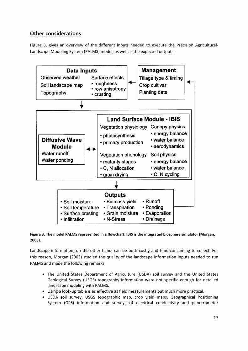
Figure 3, gives an overview of the different inputs needed to execute the Precision Agricultural‐Landscape Modeling System (PALMS) model, as well as the expected outputs.
Figure 3: The model PALMS represented in a flowchart. IBIS is the integrated biosphere simulator (Morgan, 2003).
Landscape information, on the other hand, can be both costly and time‐consuming to collect. For this reason, Morgan (2003) studied the quality of the landscape information inputs needed to run PALMS and made the following remarks.
• The United States Department of Agriculture (USDA) soil survey and the United States Geological Survey (USGS) topography information were not specific enough for detailed landscape modeling with PALMS.
• Using a look‐up table is as effective as field measurements but much more practical. • USDA soil survey, USGS topographic map, crop yield maps, Geographical Positioning
System (GPS) information and surveys of electrical conductivity and penetrometer
17
18
measurements are good enough to use as information inputs instead of costly laboratory measurements.
• The use of a multi‐scale spatial model is accurate and flexible enough to create the precision soil map needed by PALMS.
Specifically, in our research we did not use USGS topography information, as our aim was to have the most accurate information possible to make the required calculations. Field and laboratory measurements were done to obtain required inputs to the PALMS model. These include, but were not limited, to soil samples to do soil textural analysis (hydrometer method), pF (soil‐water retention), and saturated hydraulic conductivity.
An underlying assumption is that PALMS has the sensitivity to calculate differences in the water balance of a field planted in circular compared to a field planted in a linear row pattern. Our purpose was to have a management system that minimizes erosion and therefore also minimizes crop yield reduction.
Inputs measured in the laboratory were used to quantify the surface hydrology of a field planted with sorghum, in terms of infiltration, runoff and the potential reduction in soil erosion. The soil volumetric water content values obtained in the laboratory (pF curves) were used to compare calculations to measurements. In order to calibrate PALMS to our study area, some parameters were changed from the default lookup tables used by PALMS. These parameters were soil volumetric water content at field capacity (FC) and at permanent wilting point (PWP), porosity and saturated hydraulic conductivity. Topographic and textural samples were taken in the field and used as input to the model.
Calculations obtained with PALMS provided us with information regarding suitable ways of planting dryland crops in the research area. The general concept being explored is that under dryland conditions planting crops in circles will reduce soil erosion and increase infiltration of rain.
Using a model, to emulate reality, and be captured by a single model with a cause‐effect approach, can lead to erroneous conclusions. This means that the model could correctly calculate some variables, and although the model PALMS (or any other model) cannot calculate “reality” with a 100 % accuracy, it can help select the “scientific best choice” with the expectation that some of the calculated results will be close to measured values. According to (Moriasi, 2007), in general, model simulation can be judged as satisfactory if the Nash‐Sutcliffe efficiency (NSE) > 0.50 and ratio of the root mean square error to the standard deviation of measured data (RSR) is < 0.70.
Molling (2005) presented PALMS as a tool to improve both, farmer’s income and long‐term conservation. This is a model that was developed both for scientific purposes and to improve the life of farmers, and to assist in long‐term environmental management of cropping systems using a mechanistic and integrated approach.

2.3 Laboratory work
2.3.1 Textural analysis
Soil samples in the study‐field were taken with a tractor‐mounted hydraulic system using a Giddings soil core sampler (http://www.soilsample.com/). This system pushed into the soil a tube sampler with a plastic sleeve inside. Once the sampler was removed from the soil the sleeve inside the core was extracted and the soil sample obtained. This plastic sleeve was 1.2 m long and 0.05 m diameter. The soil samples were thereafter stored in a cold‐room at a temperature of 5 °C. A total of 72 samples were taken all over the field on the 15 July 2009 (see Fig. 4).
Figure 4. Textures at 0.15 m., across the study field, in Lamesa, Texas.
After the sampling process, the soil in the cores was used to identify the different soil horizons at the study‐field in Lamesa, Texas. The horizons (Table 1) were separated using a power saw to dissect the core, and the corresponding soil for each horizon was placed in bags. Thereafter the soil was oven‐dried at 105 °C for 24 hours. Once the soil samples were dry, they were ground with a mill and sieved to 2 mm, this way we made sure that only sand, silt and clay were in the sample.
Table 1. Upper and lower absolute depth limits of each soil horizon at the study‐field in Lamesa, Texas.
Horizon Upper limit (m)
Lower limit (m)
Ap1 0.0 0.3 Ap2 0.1 0.3 Bt1 0.2 0.5 Bt2 0.3 2.6 Bt3 0.4 2.6 Btk 0.5 2.6 Btkk 0.5 2.6
Once the soil samples were prepared, their particle‐size distribution, i.e., texture was measured. For this purpose, the hydrometer method (Bouyoucos, 1962) was selected and used. This method uses the Navier‐Stokes equation to calculate soil particles in suspension in an infinite soil column.
19

According to (Klute, 1986) this method is adequate for textural class identification, but cannot be used to accurately define the particle size; however, it serves the purpose of providing the textural class, which is what is needed as input to PALMS. The procedure used follows:
• Weighed 50 g of each soil sample and added 2 g of sodium hexametaphosphate, which is used as a dispersing agent to break up the soil aggregates.
• Mechanically stirred the soil and sodium hexametaphosphate, with added distilled water for 30 minutes.
• After mixing, put in a graduated cylinder and bring the solution up to a 1 L volume.
• Put a rubber stopper and shaked the cylinder end‐over‐end until all soil particles were in suspension.
• Placed cylinder on a flat surface and time for 40 seconds with the hydrometer inside (make the reading at 40 seconds). Do this twice.
• Recorded the temperature of the solution.
• Then shaked again and placed cylinder down for 2 hours.
• Took final hydrometer reading.
• Recorded temperature of the solution.
Once the readings were finished, a temperature correction was done as follows:
If the temperature was > 20 °C;
36.0)20( ⋅−+= arcr THH
Equation 1. Hydrometer reading correction with temperature (1).
If the temperature was < 20 °C,
36.0)20( ⋅−+= arcr THH
Equation 2. Hydrometer reading correction with temperature (2).
Where:
Hcr = Corrected hydrometer reading in g/L
Hr = Hydrometer reading in g/L
Ta = Temperature measured in the soil solution at 40 seconds and 2 hours, respectively, in °C.
Two samples were taken at each location (A and B). The horizons identified were Ap, Bt, Btk and Bkk.
20

2.3.2 Laboratory Permeameter Procedure (Ksat)
A sensitive parameter in hydrological models is the saturated hydraulic conductivity (Ksat), which is also one of the most problematic measurements at field‐scale in regard to variability and uncertainty (Muñoz‐Carpena et al., 2002).
The laboratory permeameter method was used to measure the saturated permeability of undisturbed soil samples in sample rings. The saturated hydraulic conductivity (Ksat) refers to the capacity of the soil to drain water and gives accurate information about the presence of disruptive soil strata, the correlation between the permeability and other soil characteristics.
The geometry of the complex pores that depend on texture, structure, viscosity and density, determine the Ksat. Saturated soil is referred to as saturated permeability. The compaction, expansion, contraction and the occupation of the absorption complex in soils, affect its permeability (anisotropy).
The laboratory permeameter operates on the basis of the principle outlined below (see Fig. 5) by creating a difference in water pressure (h) on both ends of a saturated soil sample, the water will flow through the sample and the permeability can then be calculated.
1. Storage cistern 2. Circulation pump 3. Filter 4. Adjustable water level regulator 5. Plastic container 6. Saturated ring sample inside the ringholder 7. Plastic siphon 8. Burette 9. Plastic cage (recover water)
21
Figure 5. Laboratory permeameter. Source (Eijkelkamp, 2008).
With the help of a gouge auger, a ring of undisturbed soil was taken. Two soil samples were taken at each location at 0.15 and 0.5 m depth, to sample the A and Bt horizons. The sampler ring was 0.05 m in diameter by 0.051 m long.
To avoid the possible disaggregation of soil particles in each sample, which would cause the silting of the pores and a reduction of the flow and Ksat, we prepared and used a de‐aerated solution (Klute, 1986). Ultrahigh pure water was used for this purpose. To reduce the air dissolved in the water it was autoclaved at 120 °C for 30 minutes. After that it was saturated with calcium sulphate (CaSO4

∙2H2O). The solubility of the CaSO4 is 0.0024 kg/ L at 20 °C, so to prepare 48 L, 0.15 kg were used to make sure it was completely saturated. Toluene was added to the solution (0.00021 L/L) in order to get rid of all the microorganisms that could grow in the water during the procedure.
Samples were gradually saturated to avoid the possible reduction of permeability due to encapsulation of air in the pores. The saturation was done from surface to bottom of the sample due to the fact that water would flow in that way in the permeameter. In the surface of the sample (upper part of the soil) a piece of cloth was placed to avoid the sample falling from the ring, but at the same time, allow the water to enter and saturate the sample. The sample was then placed in a ring‐holder, with a strainer cup that allowed water to flow, and taken to the plastic container (see Fig. 5). The next step was to raise the water level to create a flux of water through the sample.
In some soil samples, water flowed in the range of operation for the permeameter method, while in other samples the water flowed in the range of the constant head method. For this reason, both methods were used and matched to the values of permeability of each soil sample. Our first approach was to use the constant head method and if water flow was slow (< 1.16∙10‐7 m/s) the falling head method was selected and used.
2.3.2.1 Permeability determination: Constant head method The constant head method keeps a constant water head above the level of the water inside the ring‐holder. To avoid the water from being level with the water table and thus stop the flow, a siphon is used to connect the sample cylinders with a pipe that takes the water to a burette. With this method, the difference in volume of water drained off in time is measured (see Fig. 6). The constant head used for this purpose was from 0.017 – 0.027 m (depending on the position of the siphon in each sample, related with the water level height).
h
Burette
Siphon
Sample
A
L
Figure 6. Constant head permeameter.
Calculation
To determine permeability, Darcy’s flow equation was used to calculate the Ksat.
22

htALVKsat ⋅⋅⋅
=
Equation 3. Ksat constant head method
Where :
Ksat = Saturated Hydraulic conductivity (m/s),
A = Surface of a cross‐section of the sample (m2),
L = length of the soil sample (m),
V = Volume measured in the burette (m3), and
t = time between volume readings (s).
Water temperature affects its viscosity, and thus the Ksat. Therefore a correction for the temperature is needed. The temperature of the water in the experiments was constant 20.8 °C, and the temperature used in PALMS model for the values of Ksat was 20 °C.
2020 / hhkk TT ⋅=
Equation 4. Ksat correction with temperature
Where:
k20 = corrected Ksat at 20 °C (m/s),
kT = calculated Ksat in the experiment (m/s),
h20 = Dynamic viscosity of water at 20 °C (1.01∙10‐3 Pa.s) and
hT = Dynamic viscosity of water in the experiment 20.8 °C (0.99∙10‐3 Pa.s).
2.3.2.2 Permeability determination: Falling head method
This method consists in calculating the difference in head between the water table and the water inside the ring‐holder as a function of time. The first step is to even the water table inside the ring‐holder and outside. Once this is done, water from the ring‐holder is lowered with the siphon or a syringe. By doing this a pressure head is created that will make the water flow through the sample to even the level with the water table in the container. With the help of a measuring bridge, the difference in head can be measured, inside and outside the ring‐holder, as a function of time. In Fig. 7 the change on water level in an interval of time (t1 to t2) with the difference in head (h1 and h2 respectively) is shown. By measuring the difference in time between the two points and the
23

difference in hydraulic head (h), it is possible to calculate the Ksat. This method considers the evaporation of water inside the ring‐holder.
h1
a
A
L
Moment t1
h2
a
A
L
Moment t2
Figure 7. Water movement through soil sample. (Source: Dr. Axel Ritter, University of La Laguna, Canary Islands, Spain. Personal communication)
Calculation (Eijkelkamp, 2008)
The equation derived taking into account that the variation in h with time, which corresponds with the Darcian flow is given by:
aA
LhK
dtdh
sat ⋅−=
0≠dtdh
Equation 5. K falling head method.
Where:
Ksat = Saturated hydraulic conductivity (m/s),
a = cross‐section surface of a ring‐holder or sample cylinder (m2),
A = Surface of a cross‐section of the sample (m2), and
L= length of the soil sample (m).
Solving them for Ksat yields:
2
1
12
ln)( h
httA
LaKsat −⋅
= for h1≠h2
Equation 6. Ksat falling head method
Where:
t2 = time of second measurement (s),
t1 = time of first measurement (s),
24

h1 = head (water level difference) inside the core and the water table (outside the core) at time 1 (t1) (m), and
h2 = head (water level difference) inside the core and the water table (outside the core) at time 2 (t2) (m).
Once the Ksat is known it has to be corrected with the evaporation in the interval time (t1 ‐ t2) as follows:
)(ln
)( 212
1
12 hhALax
hh
ttALaKsat ⋅⋅
⋅⋅+⋅
−⋅⋅
=
Equation 7. Ksat falling head method.
Where:
x = evaporation factor (1∙10‐8 m/s) (Eijkelkamp, 2008),
2.3.3 Water retention curve determination
To determine the water retention curve, the Mualem‐van Genuchten equation was used:
( )[ ] pnn
ps hh θαθθθ +⋅+⋅= −11
)1)()(
Equation 8. Van Genuchten Equation according to Mualem’s theory (van Genuchten, 1980).
Where:
Θ = Volumetric water content (m3/m3),
Θs= Saturated water content (m3/m3),
Θp = Residual water content (m3/m3).
h = Suction (cm), and
α and “m” = Curve‐shape parameters.
2.3.3.1 Sand/Kaolin box, 0 – 50 kPa (Eijkelkamp, 2005b)
The soil samples that were first used to measure Ksat, were kept moist close to saturation and then taken to the sand/kaolin box to determine the water retention curves. Samples were placed with the bottom side down in the sand/kaolin box for 1 h. After that, more water (de‐mineralized) was poured onto the kaolin surface to reach ~ 3/4 of the sample’s height. In this moment samples were
25

at saturation, so they were weighted with a balance to an accuracy of ± 0.00001 kg, to obtain water content at pF = 0. It was noted that this measurements at pF = 0 were inaccurate, as drops were falling from the sample when weighing them. Also, the middle of the sample was used as the reference level for zero pressure, but the free water level (h = 0) was in fact 1 cm below the top of the sample ring. The moisture tension thus is different at the bottom (+ 4 cm) than at the top of the sample (‐ 1 cm). After 2‐3 days, the water level reached the surface of the kaolin. Then suctions of 0.25 kPa (pF = 0.4), 6 kPa (pF = 1.78), 10 kPa (pF = 2), 33 kPa (pF = 2.52) and 50 kPa (pF = 2.7) were set. For every step, 3 days were needed to pass to reach a steady state (this happened when we had about the same weight in 2 different weighings with the same suction), after that point, the next suction was set.
Once we had the weights of the soil samples the following calculations were done:
w
sw
SWW %100⋅
=
Equation 9. Gravimetric water content.
Where:
W = Gravimetric water content (kg of water in the soil /kg of soil),
Wsw= Weight of soil water (kg) = weight of wet sample – weight of dry sample, and
Sw= Soil weight (kg) = weight of dry sample (without the ring, cloth and elastic).
The dry bulk density (ρd) of the soil is an important site‐specific property, since it changes for a given soil. It varies with structural condition of the soil, particularly that related to packing. A very important parameter to calculate is the ρd, which is defined as the ratio of the mass of dry solids in kg (Wds) to the bulk volume of the soil occupied by those dry solids in m3 (V).
VWds
d =ρ
Equation 10, Dry bulk density.
The volumetric water content (θ) was calculated as follows (assuming water density as 1000 kg/m3):
dw ρθ ⋅=
Equation 11. Volumetric water content.
Where:
θ = Volumetric water content (m3 of water / m3 of soil),
W = Gravimetric water content (kg/kg), and
ρd = Soil dry bulk density (kg/m3).
26

2.3.3.2 Pressure membrane apparatus, 1500 kPa (Eijkelkamp, 2005a)
For a pF = 4.18 (1500 kPa ≈ 15 bar) the water in the soil is retained in very small pores, meaning that the soil water retention is dominantly influenced by soil texture. For this reason, disturbed soil samples can be used for this determination.
Disturbed soil samples were wetted with enough water to saturate the samples for 2‐3 days. After that, three rings (0.0355 m in diameter and 0.0101 m height) for an ~ volume of 1∙10‐5 m3, were filled with soil and placed in the pressure‐plate apparatus. Then a pressure of 1500 kPa was applied for three days to the three replicates that were used for each sample. Afterwards soil samples were weighed (wet weight), oven‐dried at 105 °C and weighed again (dry weight). With these values the
soil’s volumetric water content, was calculated for a pF = 4.18, using the ρd of the undisturbed samples used in the sand/kaolin box.
2.4 Model performance evaluation
To evaluate calculated values obtained with PALMS model and compare them to corresponding measured values, we selected the following three statistical parameters, RMSD, NSE, and RSR, which are described as follows.
• The root mean squared deviation (RMSD) (Kobayashi and Salam, 2000). It gives the mean difference between measured and calculated values
( )∑=
−=n
iii yx
nRMSD
1
21
Equation 12. Root mean squared deviation (RMSD) equation.
Where:
Xi = measured value and the corresponding calculated value is Yi.
• The Nash Sutcliffe efficiency (NSE) was also used (Moriasi, 2007) to compared measured and calculated values.
( )( ) ⎥⎥
⎥⎥
⎦
⎤
⎢⎢⎢⎢
⎣
⎡
−
−−=
∑
∑
=
=n
i
meani
obsi
n
i
simi
obsi
YY
YYNSE
1
2
1
2
1
Equation 13. Nash Sutcliffe efficiency (NSE) equation.
Where:
27

Yiobs= Measurement for the constituent being evaluated,
Yisim= Calculated value for the constituent being evaluated,
Yimean= Mean measured data for the constituent being evaluated, and
n = total number of observations.
The Nash–Sutcliffe efficiencies may range from −∞ to 1. An efficiency of 1 (NSE = 1) corresponds to a
perfect match of modeled compared to the measured values. An efficiency of 0 (NSE = 0) indicates
that the model calculations are as accurate as the mean of the measured data, whereas an efficiency
< 0 (NSE < 0) occurs when the measured mean is a better predictor than the model or, in other
words, when the residual variance (described by the nominator in the expression above), is larger
than the data variance (described by the denominator).
• Ratio of the mean squared error to the standard deviation of measured data (RSR).
( )
( )⎥⎥⎦
⎤
⎢⎢⎣
⎡−
⎥⎥⎦
⎤
⎢⎢⎣
⎡−
=
∑
∑
=
=
n
i
meani
obsi
n
i
simi
obsi
YY
YYRSR
1
2
1
2
Equation 14. Ratio of the mean squared error to the standard deviation of measured data (RSR) equation
The RSR incorporates the benefit of error index statistics and has an optimal value of 0.
28
29
3. Results and Discussion
3.1 Laboratory Results
3.1.1 Textures (hydrometer method)
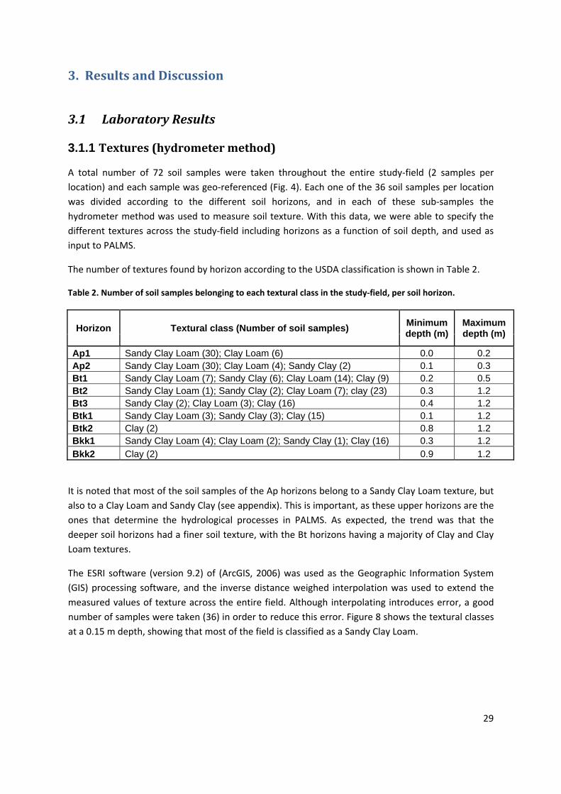
A total number of 72 soil samples were taken throughout the entire study‐field (2 samples per location) and each sample was geo‐referenced (Fig. 4). Each one of the 36 soil samples per location was divided according to the different soil horizons, and in each of these sub‐samples the hydrometer method was used to measure soil texture. With this data, we were able to specify the different textures across the study‐field including horizons as a function of soil depth, and used as input to PALMS.
The number of textures found by horizon according to the USDA classification is shown in Table 2.
Table 2. Number of soil samples belonging to each textural class in the study‐field, per soil horizon.
Horizon Textural class (Number of soil samples) Minimum depth (m)
Maximum depth (m)
Ap1 Sandy Clay Loam (30); Clay Loam (6) 0.0 0.2 Ap2 Sandy Clay Loam (30); Clay Loam (4); Sandy Clay (2) 0.1 0.3 Bt1 Sandy Clay Loam (7); Sandy Clay (6); Clay Loam (14); Clay (9) 0.2 0.5 Bt2 Sandy Clay Loam (1); Sandy Clay (2); Clay Loam (7); clay (23) 0.3 1.2 Bt3 Sandy Clay (2); Clay Loam (3); Clay (16) 0.4 1.2 Btk1 Sandy Clay Loam (3); Sandy Clay (3); Clay (15) 0.1 1.2 Btk2 Clay (2) 0.8 1.2 Bkk1 Sandy Clay Loam (4); Clay Loam (2); Sandy Clay (1); Clay (16) 0.3 1.2 Bkk2 Clay (2) 0.9 1.2
It is noted that most of the soil samples of the Ap horizons belong to a Sandy Clay Loam texture, but also to a Clay Loam and Sandy Clay (see appendix). This is important, as these upper horizons are the ones that determine the hydrological processes in PALMS. As expected, the trend was that the deeper soil horizons had a finer soil texture, with the Bt horizons having a majority of Clay and Clay Loam textures.
The ESRI software (version 9.2) of (ArcGIS, 2006) was used as the Geographic Information System (GIS) processing software, and the inverse distance weighed interpolation was used to extend the measured values of texture across the entire field. Although interpolating introduces error, a good number of samples were taken (36) in order to reduce this error. Figure 8 shows the textural classes at a 0.15 m depth, showing that most of the field is classified as a Sandy Clay Loam.

Figure 8. Textures at 0.15 m depth across the study‐field, in Lamesa, Texas.
The field has five distinct areas (see Fig. 4) with oil wells and access roads that are not cultivated. However, these areas were included in our analysis as they contribute to the hydrological processes of the entire field, and thus we assigned a textural class of Sandy Clay to the soil profile at these locations. The end result is that these areas play an important role in the runoff processes, which is probably closer to reality.
In Fig. 9 the textural classes presented at a 0.5 m depth is shown. Please note the abundance of clay texture at this depth.
Clay LoamSandy Clay
Figure 9. Textures at 0.5 m depth across the study‐field, in Lamesa, Texas.
30

The topographic map was done from data obtained by j. Randall Nelson on March 2009. A total number of 4754 spots with coordinates and altitudes were taken and afterwards interpolated using ArcGIS to create the topographic map (see Fig. 10).
31
figure 9).
831.9 - 832.5
832.5 - 833
833 - 833.5
833.5 - 834
834 - 834.5
834.5 - 835
835 - 835.5
µ835.5 - 836
Figure 10. The 3D Topographic map (m.a.s.l.), the vertical scale is exaggerated 20X to enable differenting the sloppier locations. Data from j. Randall Nelson (March, 2009).
As it can be seen in Fig. 10, the field is relatively level. The maximum slope is 5 % but the average slope is 0.33 % (see Fig. 11), which directly affects the surface hydraulic processes, such as runoff and infiltration.
Slope (%
)
0.001 - 0.2
0.2 - 1
1 - 2
2 - 3
3 - 4
4 - 5
Figure 11. Slope map of the study‐field in Lamesa, Texas.
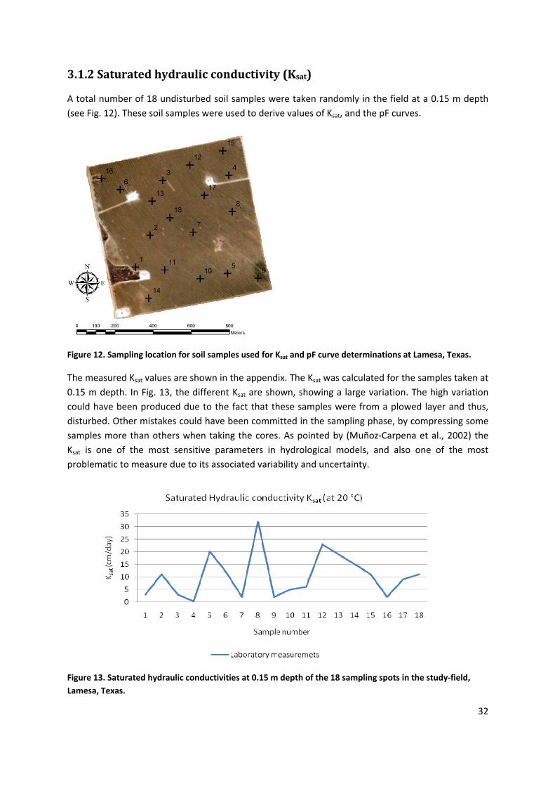
3.1.2 Saturated hydraulic conductivity (Ksat)
A total number of 18 undisturbed soil samples were taken randomly in the field at a 0.15 m depth (see Fig. 12). These soil samples were used to derive values of Ksat, and the pF curves.
Figure 12. Sampling location for soil samples used for Ksat and pF curve determinations at Lamesa, Texas.
The measured Ksat values are shown in the appendix. The Ksat was calculated for the samples taken at 0.15 m depth. In Fig. 13, the different Ksat are shown, showing a large variation. The high variation could have been produced due to the fact that these samples were from a plowed layer and thus, disturbed. Other mistakes could have been committed in the sampling phase, by compressing some samples more than others when taking the cores. As pointed by (Muñoz‐Carpena et al., 2002) the Ksat is one of the most sensitive parameters in hydrological models, and also one of the most problematic to measure due to its associated variability and uncertainty.
Figure 13. Saturated hydraulic conductivities at 0.15 m depth of the 18 sampling spots in the study‐field, Lamesa, Texas.
32

33
3.1.3 Soil water retention
There were 3 textures represented in the 18 undisturbed soil samples, used to determine the pF water retention curves. i.e., Clay loam (CL), Sandy Clay Loam (SCL) and Sandy Clay (SC). There were 13 samples of SCL, 4 of CL and 1 SC. According to the most frequent values presented for each sample of each textural class, Table 3 shows the soil volumetric water content (VWC) as a function of pressure applied.
Table 3. Soil volumetric water content (m3/m3) per texture and suction value for soils from the study‐field, Lamesa, Texas.
Texture Suction (kPa)
0 0.25 6 10 33 (FC) 50 1500 (PWP)
Clay Loam 0.45 0.47 0.40 0.36 0.30 0.28 0.17
Sandy Clay 0.49 0.49 0.41 0.37 0.27 0.25 0.14
Sandy Clay Loam 0.45 0.46 0.42 0.40 0.29 0.28 0.15
The SC is capable of retaining more water at saturation and this is probably related to the porosity, which is also the highest (45.5 %) among the soil samples taken, and also its Ksat was the fastest (see appendix). The soil volumetric water content at Field capacity (FC) and Permanent wilting point (PWP) were used in the calibration of the model.
Following the same procedure used to determine the better choice for the soil VWC of each texture,
the most frequent bulk densities (ρb) were selected for each textural class and its porosity was calculated (assuming particle density of 2650 kg/m3). These results are shown in Table 4.
Table 4. Bulk densities and porosity of the textural classes in the study‐field, Lamesa, Texas.
Textural Class ρb
Bulk density (kg/m3) Porosity (%)
Clay Loam 1600 39.6
Sandy Clay 1400 45.5
Sandy Clay Loam 1700 35.8
The SC had the lowest ρb and thus the highest porosity. The high values of ρb in the SCL samples lowered the calculated porosity affecting the hydraulic properties of the corresponding horizon.
With the data given in Table 3 the Mualem‐Van Genuchten equation was adjusted for every soil textural class found in the study‐field in Lamesa, Texas.
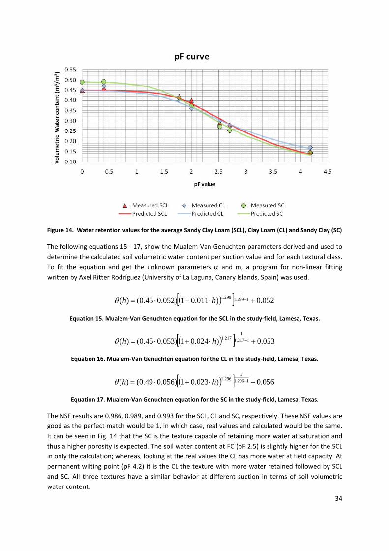
Figure 14. Water retention values for the average Sandy Clay Loam (SCL), Clay Loam (CL) and Sandy Clay (SC)
The following equations 15 ‐ 17, show the Mualem‐Van Genuchten parameters derived and used to determine the calculated soil volumetric water content per suction value and for each textural class.
To fit the equation and get the unknown parameters α and m, a program for non‐linear fitting written by Axel Ritter Rodríguez (University of La Laguna, Canary Islands, Spain) was used.
( )[ ] 052.0)011.01)052.045.0()( 1299.11
299.1 +⋅+⋅= −hhθ
Equation 15. Mualem‐Van Genuchten equation for the SCL in the study‐field, Lamesa, Texas.
( )[ ] 053.0)024.01)053.045.0()( 1217.11
217.1 +⋅+⋅= −hhθ
Equation 16. Mualem‐Van Genuchten equation for the CL in the study‐field, Lamesa, Texas.
( )[ ] 056.0)023.01)056.049.0()( 1296.11
296.1 +⋅+⋅= −hhθ
Equation 17. Mualem‐Van Genuchten equation for the SC in the study‐field, Lamesa, Texas.
The NSE results are 0.986, 0.989, and 0.993 for the SCL, CL and SC, respectively. These NSE values are good as the perfect match would be 1, in which case, real values and calculated would be the same. It can be seen in Fig. 14 that the SC is the texture capable of retaining more water at saturation and thus a higher porosity is expected. The soil water content at FC (pF 2.5) is slightly higher for the SCL in only the calculation; whereas, looking at the real values the CL has more water at field capacity. At permanent wilting point (pF 4.2) it is the CL the texture with more water retained followed by SCL and SC. All three textures have a similar behavior at different suction in terms of soil volumetric water content.
34

3.2 Rosetta simulation
Due to the high variability obtained for the measured Ksat values and to evaluate how well a pedotransfer function worked in the study‐field, we decided to use the model Rosetta (Schaap et al., 2001) to calculate soil hydraulic properties from surrogate soil data. The values of percentage of clay, silt and sand, bulk density, and water retention at field capacity (33 kPa), and permanent wilting point (1500 kPa) measured on each of the 18 soil samples used to measure Ksat were used as input to Rosetta.
Soil sample number 8 corresponded to SC; whereas, 2, 7, 9 and 13 belonged to a CL. The rest of the soil samples (1, 3, 4, 5, 6, 10, 11, 12, 14, 15, 16, 17 and 18) were SCL.
Figure 15. Saturated hydraulic conductivity (Ksat) measured compared to Rosetta calculations.
From Fig. 15, it is clear that the SC sample (8) has the higher Ksat, whereas the CL (2, 7, 9, 13) are as random as the SCL. It can be seen that Rosetta tends to overestimate the values of Ksat, but in general it follows the same pattern of the measured data.
The RMSD for the Ksat is 6.7, which is the mean difference between measured and calculated values obtained with Rosetta. This is a relatively high value; however,if the large variability of the measured values is considered and we compare the measured Ksat values for the same texture, the difference among them (from 2 to 23 cm/day for SCL) is higher that the RMSD. This finding and the fact that the pattern calculated by Rosetta was similar to the one obtained from measured values on all soil samples of the study‐field, suggests that Rosetta could be used in the abscense of measured values.
35
36
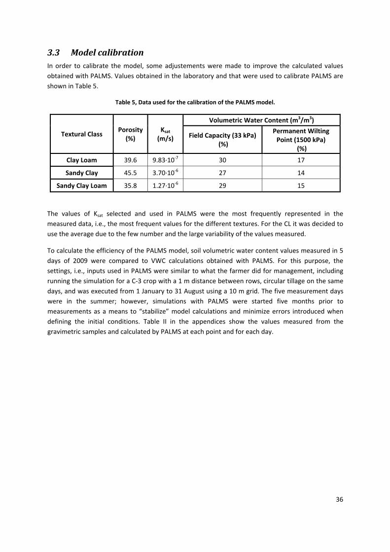
3.3 Model calibration In order to calibrate the model, some adjustements were made to improve the calculated values obtained with PALMS. Values obtained in the laboratory and that were used to calibrate PALMS are shown in Table 5.
Table 5, Data used for the calibration of the PALMS model.
Textural Class Porosity
(%) Ksat (m/s)
Volumetric Water Content (m3/m3)
Field Capacity (33 kPa) (%)
Permanent Wilting Point (1500 kPa)
(%)
Clay Loam 39.6 9.83∙10‐7 30 17
Sandy Clay 45.5 3.70∙10‐6 27 14
Sandy Clay Loam 35.8 1.27∙10‐6 29 15
The values of Ksat selected and used in PALMS were the most frequently represented in the measured data, i.e., the most frequent values for the different textures. For the CL it was decided to use the average due to the few number and the large variability of the values measured.
To calculate the efficiency of the PALMS model, soil volumetric water content values measured in 5 days of 2009 were compared to VWC calculations obtained with PALMS. For this purpose, the settings, i.e., inputs used in PALMS were similar to what the farmer did for management, including running the simulation for a C‐3 crop with a 1 m distance between rows, circular tillage on the same days, and was executed from 1 January to 31 August using a 10 m grid. The five measurement days were in the summer; however, simulations with PALMS were started five months prior to measurements as a means to “stabilize” model calculations and minimize errors introduced when defining the initial conditions. Table II in the appendices show the values measured from the gravimetric samples and calculated by PALMS at each point and for each day.
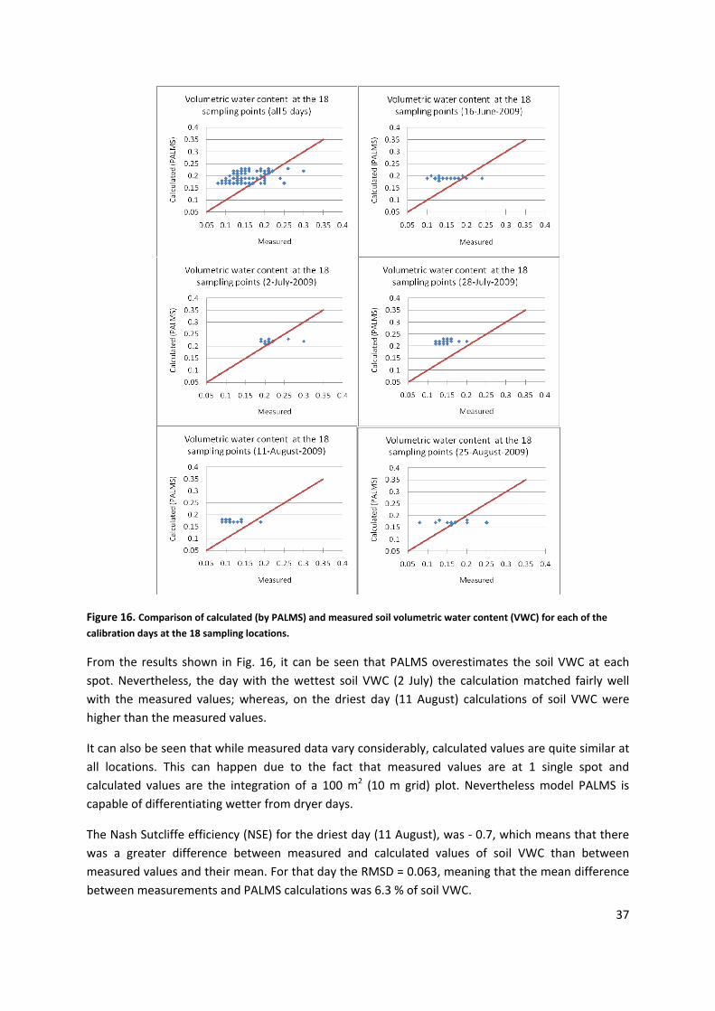
Figure 16. Comparison of calculated (by PALMS) and measured soil volumetric water content (VWC) for each of the
calibration days at the 18 sampling locations.
From the results shown in Fig. 16, it can be seen that PALMS overestimates the soil VWC at each spot. Nevertheless, the day with the wettest soil VWC (2 July) the calculation matched fairly well with the measured values; whereas, on the driest day (11 August) calculations of soil VWC were higher than the measured values.
It can also be seen that while measured data vary considerably, calculated values are quite similar at all locations. This can happen due to the fact that measured values are at 1 single spot and calculated values are the integration of a 100 m2 (10 m grid) plot. Nevertheless model PALMS is capable of differentiating wetter from dryer days.
The Nash Sutcliffe efficiency (NSE) for the driest day (11 August), was ‐ 0.7, which means that there was a greater difference between measured and calculated values of soil VWC than between measured values and their mean. For that day the RMSD = 0.063, meaning that the mean difference between measurements and PALMS calculations was 6.3 % of soil VWC.
37
38
Conversely, in the day with the wettest soil VWC (2 July), NSE = 0.81, which means that the model calculations are better that the average of the measured values. The RMSD = 0.025, so the mean difference between the measured data and the calculated values is 2.5 % of the soil VWC. The ratio of the root mean square error to the standard deviation of measured data (RSR) in this case was 0.43, and according to (Moriasi, 2007) the calculated values obtained with PALMS can be classified as satisfactory, i.e., NSE > 0.50 and RSR < 0.70.
The overall NSE = ‐0.53 and the overall RMSD = 0.054 (5.4% soil VWC). These results suggest that PALMS performed better under conditions where the soil VWC is not close to the permanent wilting point. Out of the five days we compared measured and calculated values, in three of them (16 June,
11 and 28 August) most of the measured values were ≤ the PWP and thus the overall performance of PALMS tended to be lower. Furthermore, this comparison is for a point measurement, i.e., single depth and time, in the profile and perhaps is not indicative of the overall performance of PALMS to calculate the total amount of water in the soil profile. This comparison also suggests that a more dense measurement of soil VWC is required to further test the model and that given the spatial variability of soil VWC the measurement of choice for this type of field application is the neutron attenuation method to measure soil VWC (Evett et al., 2006). Further, the PALMS model does not take into account differences of organic matter across field, and thus this could be adding error to the calculations. However, this effect might be minimal given the low organic matter of this field.
The accuracy of any soil VWC measurement is ± 3 to 5%, depending on the measurement method (C. Molling, personal communication), so overall results obtained with PALMS, given the range of soil VWC measurements, is encouraging. Furthermore, these results suggest that PALMS calculations are subject to “less” error under wet soil conditions so we can infer that algorithms used to calculate soil erosion would also follow the same trend. Nevertheless, further experimental verification for different soil types and conditions are needed to properly evaluate PALMS.
3.4 Model validation Once PALMS was calibrated, it was then used to simulate the year 2008, in which the study‐field Lamesa, Texas was planted with a Sorghum crop in a circular pattern. Although calculations obtained with the PALMS model are subject to errors, the results obtained may nevertheless provide a “relative” estimate of erosion, runoff and infiltration when comparing circular vs. straight planting pattern. Furthermore, the calculated values obtained with PALMS can guide further research and provides us with a valuable tool to target specific field measurements that can be used in validation of the model.
3.4.1 Infiltration
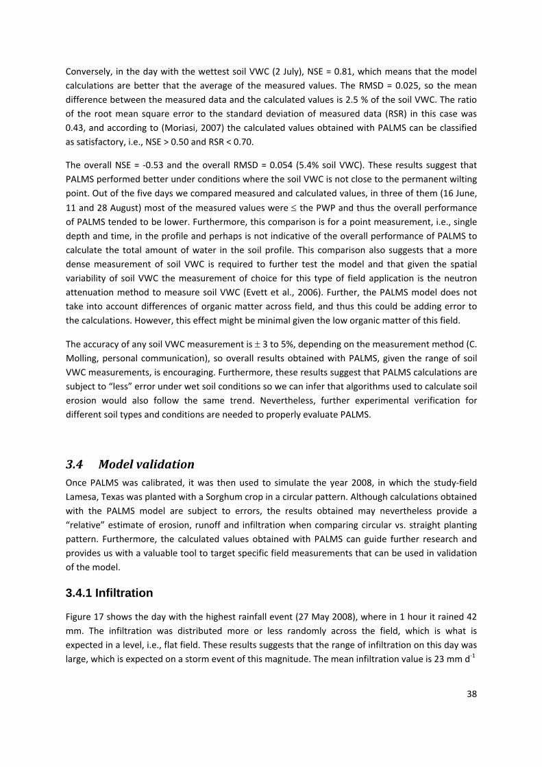
Figure 17 shows the day with the highest rainfall event (27 May 2008), where in 1 hour it rained 42 mm. The infiltration was distributed more or less randomly across the field, which is what is expected in a level, i.e., flat field. These results suggests that the range of infiltration on this day was large, which is expected on a storm event of this magnitude. The mean infiltration value is 23 mm d‐1
In order to quantify the differences between straight vs. circular rows operations across the study‐field, the infiltration amount from the circular rows were subtracted from the corresponding straight rows (straight – circular) and this result is shown in Fig. 18.
39
55.2 mm d‐1
14.6 mm d‐1
Figure 17. Infiltration simulated with a circular row pattern on the 27 May 2008 at the study‐field, Lamesa, Texas.
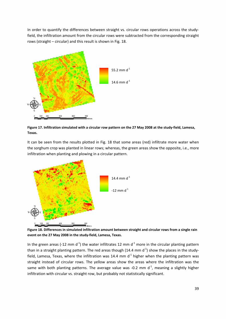
It can be seen from the results plotted in Fig. 18 that some areas (red) infiltrate more water when the sorghum crop was planted in linear rows; whereas, the green areas show the opposite, i.e., more infiltration when planting and plowing in a circular pattern.
Figure 18. Differences in simulated infiltration amount between straight and circular rows from a single rain event on the 27 May 2008 in the study‐field, Lamesa, Texas.
14.4 mm d‐1
‐12 mm d‐1
In the green areas (‐12 mm d‐1) the water infiltrates 12 mm d‐1 more in the circular planting pattern than in a straight planting pattern. The red areas though (14.4 mm d‐1) show the places in the study‐field, Lamesa, Texas, where the infiltration was 14.4 mm d‐1 higher when the planting pattern was straight instead of circular rows. The yellow areas show the areas where the infiltration was the same with both planting patterns. The average value was ‐0.2 mm d‐1, meaning a slightly higher infiltration with circular vs. straight row, but probably not statistically significant.
The infiltration of water into the soil was compared based on the average infiltration per day of the highest infiltration events (in the whole field). Adding all the events, the straight planting pattern added 250 mm yr‐1 (for all the precipitation events > 4 mm h‐1); whereas, the circular planting pattern added essentially the same amount, 254 mm yr‐1. In general, there were no differences in the amount of infiltration between the linear and circular rows. However, the spatial differences indicate that parts of the field, those at a lower elevation, tended to have larger infiltration amounts. In the context of dryland farming this result is of importance as it suggests that perhaps when rain events are integrated over the growing season the benefit of additional stored soil water would translate to higher crop yields as shown by (Li et al., 2001). However, at this time this conclusion is speculative and requires experimental verification.
3.4.2 Runoff
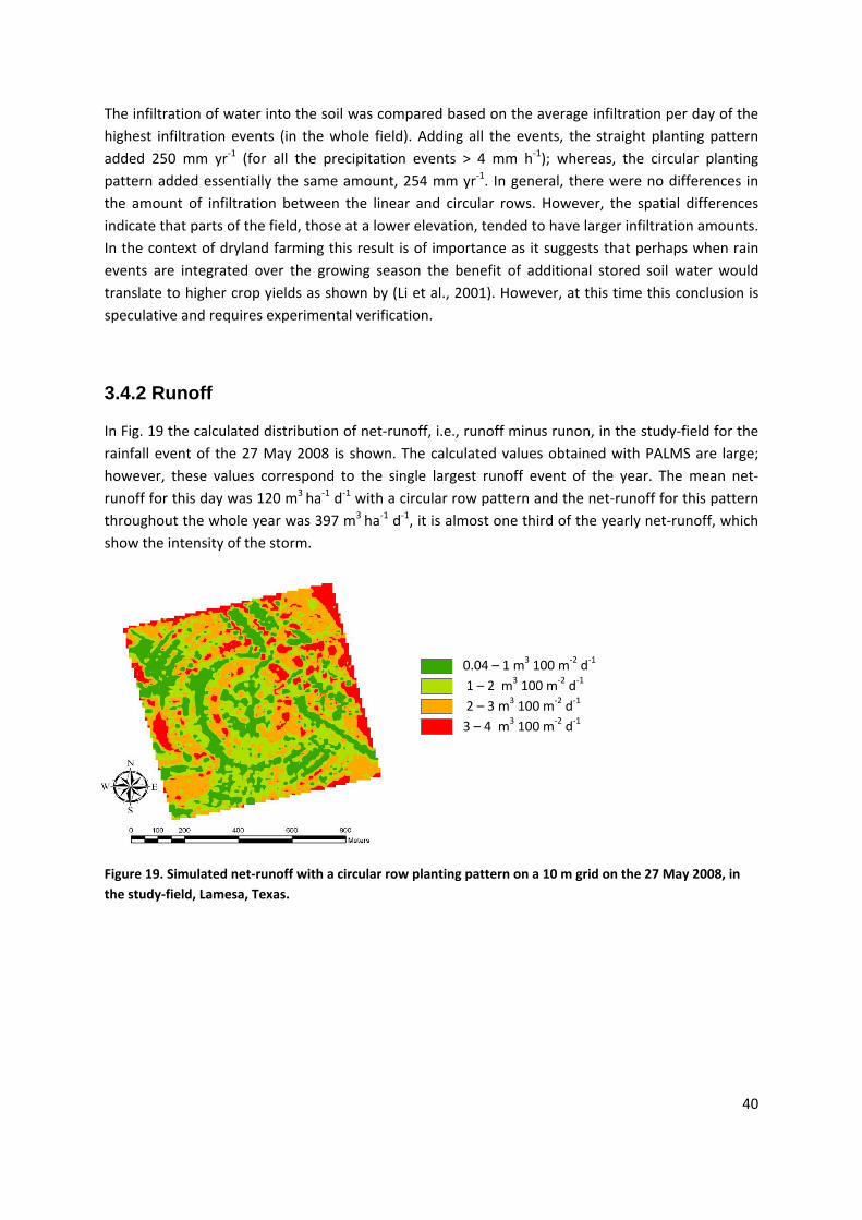
In Fig. 19 the calculated distribution of net‐runoff, i.e., runoff minus runon, in the study‐field for the rainfall event of the 27 May 2008 is shown. The calculated values obtained with PALMS are large; however, these values correspond to the single largest runoff event of the year. The mean net‐runoff for this day was 120 m3 ha‐1 d‐1 with a circular row pattern and the net‐runoff for this pattern throughout the whole year was 397 m3 ha‐1 d‐1, it is almost one third of the yearly net‐runoff, which show the intensity of the storm.
0.04 – 1 m3 100 m‐2 d‐1
1 – 2 m3 100 m‐2 d‐1
2 – 3 m3 100 m‐2 d‐1
3 – 4 m3 100 m‐2 d‐1
Figure 19. Simulated net‐runoff with a circular row planting pattern on a 10 m grid on the 27 May 2008, in the study‐field, Lamesa, Texas.
40
‐1.6 ‐ ‐0.2 m 100 m d‐0.2 ‐ 0.06 m3 100 m‐2 d‐1
0.06 – 0.3 m3 100 m‐2 d‐1
0.3 – 1.6 m3 100 m‐2 d‐1
3 ‐2 ‐1
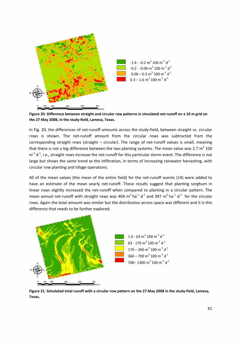
Figure 20. Difference between straight and circular row patterns in simulated net‐runoff on a 10 m grid on the 27 May 2008, in the study‐field, Lamesa, Texas.
In Fig. 20, the differences of net‐runoff amounts across the study‐field, between straight vs. circular rows is shown. The net‐runoff amount from the circular rows was subtracted from the corresponding straight rows (straight – circular). The range of net‐runoff values is small, meaning that there is not a big difference between the two planting systems. The mean value was 2.7 m3 100 m‐2 d‐1, i.e., straight rows increase the net‐runoff for this particular storm event. The difference is not large but shows the same trend as the infiltration, in terms of increasing rainwater harvesting, with circular row planting and tillage operations.
All of the mean values (the mean of the entire field) for the net‐runoff events (14) were added to have an estimate of the mean yearly net‐runoff. These results suggest that planting sorghum in linear rows slightly increased the net‐runoff when compared to planting in a circular pattern. The mean annual net‐runoff with straight rows was 404 m3 ha‐1 d‐1 and 397 m3 ha‐1 d‐1 for the circular rows. Again the total amount was similar but the distribution across space was different and it is this difference that needs to be further explored.
1.6 ‐ 63 m3 100 m‐2 d‐1
63 ‐ 170 m3 100 m‐2 d‐1
170 – 360 m3 100 m‐2 d‐1
360 – 700 m3 100 m‐2 d‐1
700– 1300 m3 100 m‐2 d‐1
Figure 21. Simulated total runoff with a circular row pattern on the 27 May 2008 in the study‐field, Lamesa, Texas.
41
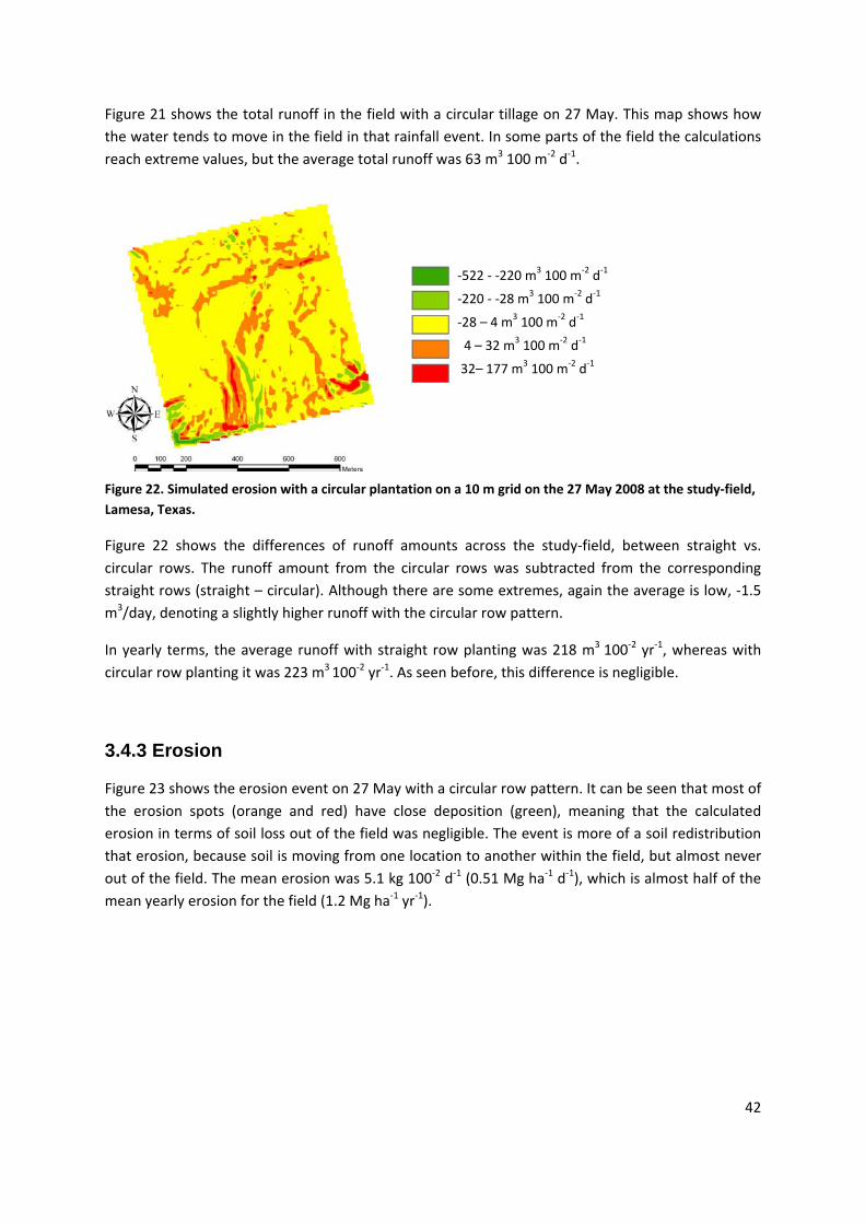
Figure 21 shows the total runoff in the field with a circular tillage on 27 May. This map shows how the water tends to move in the field in that rainfall event. In some parts of the field the calculations reach extreme values, but the average total runoff was 63 m3 100 m‐2 d‐1.
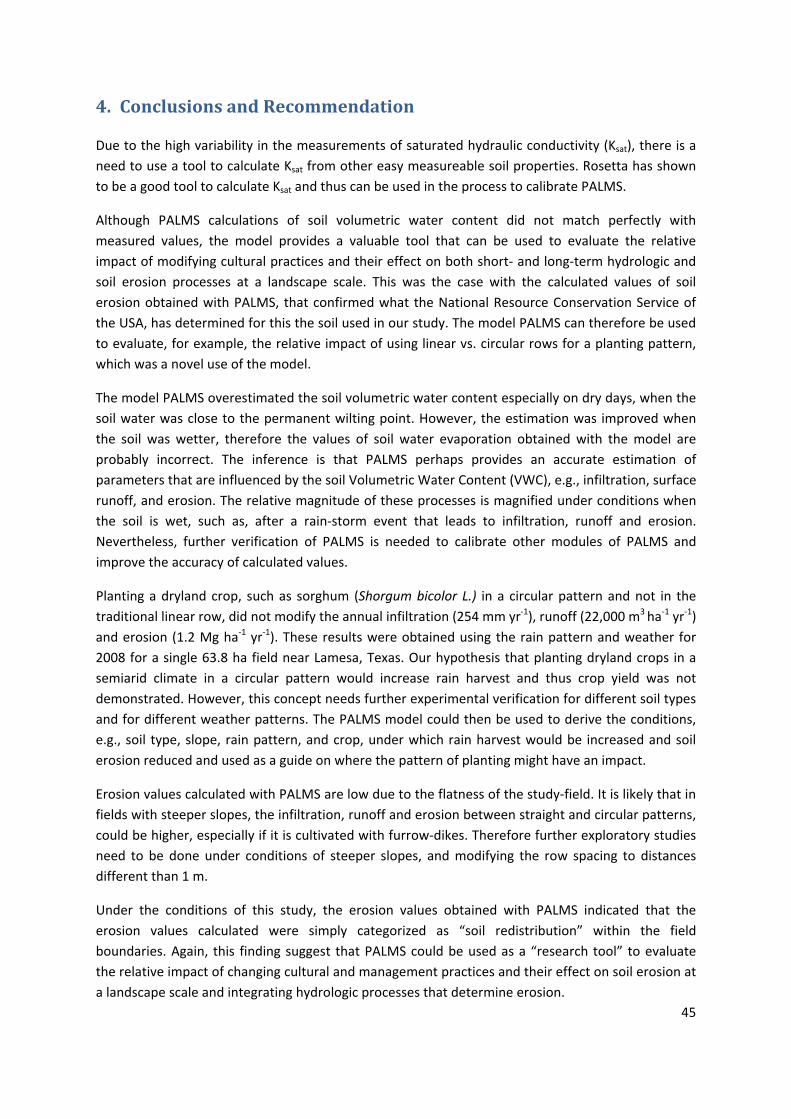
‐522 ‐ ‐220 m3 100 m‐2 d‐1
‐220 ‐ ‐28 m3 100 m‐2 d‐1
‐28 – 4 m3 100 m‐2 d‐1
4 – 32 m3 100 m‐2 d‐1
32– 177 m3 100 m‐2 d‐1
Figure 22. Simulated erosion with a circular plantation on a 10 m grid on the 27 May 2008 at the study‐field, Lamesa, Texas.
Figure 22 shows the differences of runoff amounts across the study‐field, between straight vs. circular rows. The runoff amount from the circular rows was subtracted from the corresponding straight rows (straight – circular). Although there are some extremes, again the average is low, ‐1.5 m3/day, denoting a slightly higher runoff with the circular row pattern.
In yearly terms, the average runoff with straight row planting was 218 m3 100‐2 yr‐1, whereas with circular row planting it was 223 m3 100‐2 yr‐1. As seen before, this difference is negligible.
3.4.3 Erosion
Figure 23 shows the erosion event on 27 May with a circular row pattern. It can be seen that most of the erosion spots (orange and red) have close deposition (green), meaning that the calculated erosion in terms of soil loss out of the field was negligible. The event is more of a soil redistribution that erosion, because soil is moving from one location to another within the field, but almost never out of the field. The mean erosion was 5.1 kg 100‐2 d‐1 (0.51 Mg ha‐1 d‐1), which is almost half of the mean yearly erosion for the field (1.2 Mg ha‐1 yr‐1).
42

1,000 – 3,830 kg 100 m‐2 d‐1
‐3,909 ‐ ‐1,600 kg 100 m‐2 d‐1
‐1600 ‐ ‐300 kg 100 m‐2 d‐1
‐300 – 200 kg 100 m‐2 d‐1
200 – 1,000 kg 100 m‐2 d‐1
Figure 23. Simulated erosion with a circular plantation on a 10 m grid on the 27 May 2008 at the study‐field, Lamesa, Texas.
The range of erosion values comparing the difference between straight minus circular rows (Fig. 24) seem large, especially in the southern part of the field where the slope is larger. The average value nevertheless is 0.42 kg/day (0.042 Mg/ha and day), confirming the small difference between the two planting patterns.
Figure 24. Difference between straight and circular plantation in simulated erosion on a 10 m grid on the 27 May 2008, in the study‐field, Lamesa, Texas.
‐987‐ 360 kg 100 m‐2 d‐1
‐360 ‐ ‐75 kg 100 m‐2 d‐1
‐75 – 75 kg 100 m‐2 d‐1
75 – 360 kg 100 m‐2 d‐1
360 – 1,072 kg 100 m‐2 d‐1
The erosion was also compared for the two planting patterns, i.e., straight vs. circular and tillage operation, to evaluate the process for one year. All the erosion event days (14) were added. The result shows that straight rows and tillage operations have an annual average of 1.3 Mg ha‐1 yr‐1; whereas, the circular system had a similar value of 1.2 Mg ha‐1 yr‐1. As expected and as with infiltration and runoff, the erosion is slightly reduced with a circular pattern, but these differences are not statistically different. The calculated values of erosion obtained with PALMS are small, which are probably close to reality due to the slope of the field. Furthermore, and according to (NRCS,
43

44
2008) the erosion for this soil type is negligible on 0 to 1 % slopes and low on 1 to 5 % slopes, which is in accordance to the values calculated with PALMS.
45
4. Conclusions and Recommendation
Due to the high variability in the measurements of saturated hydraulic conductivity (Ksat), there is a need to use a tool to calculate Ksat from other easy measureable soil properties. Rosetta has shown to be a good tool to calculate Ksat and thus can be used in the process to calibrate PALMS.
Although PALMS calculations of soil volumetric water content did not match perfectly with measured values, the model provides a valuable tool that can be used to evaluate the relative impact of modifying cultural practices and their effect on both short‐ and long‐term hydrologic and soil erosion processes at a landscape scale. This was the case with the calculated values of soil erosion obtained with PALMS, that confirmed what the National Resource Conservation Service of the USA, has determined for this the soil used in our study. The model PALMS can therefore be used to evaluate, for example, the relative impact of using linear vs. circular rows for a planting pattern, which was a novel use of the model.
The model PALMS overestimated the soil volumetric water content especially on dry days, when the soil water was close to the permanent wilting point. However, the estimation was improved when the soil was wetter, therefore the values of soil water evaporation obtained with the model are probably incorrect. The inference is that PALMS perhaps provides an accurate estimation of parameters that are influenced by the soil Volumetric Water Content (VWC), e.g., infiltration, surface runoff, and erosion. The relative magnitude of these processes is magnified under conditions when the soil is wet, such as, after a rain‐storm event that leads to infiltration, runoff and erosion. Nevertheless, further verification of PALMS is needed to calibrate other modules of PALMS and improve the accuracy of calculated values.
Planting a dryland crop, such as sorghum (Shorgum bicolor L.) in a circular pattern and not in the traditional linear row, did not modify the annual infiltration (254 mm yr‐1), runoff (22,000 m3 ha‐1 yr‐1) and erosion (1.2 Mg ha‐1 yr‐1). These results were obtained using the rain pattern and weather for 2008 for a single 63.8 ha field near Lamesa, Texas. Our hypothesis that planting dryland crops in a semiarid climate in a circular pattern would increase rain harvest and thus crop yield was not demonstrated. However, this concept needs further experimental verification for different soil types and for different weather patterns. The PALMS model could then be used to derive the conditions, e.g., soil type, slope, rain pattern, and crop, under which rain harvest would be increased and soil erosion reduced and used as a guide on where the pattern of planting might have an impact.
Erosion values calculated with PALMS are low due to the flatness of the study‐field. It is likely that in fields with steeper slopes, the infiltration, runoff and erosion between straight and circular patterns, could be higher, especially if it is cultivated with furrow‐dikes. Therefore further exploratory studies need to be done under conditions of steeper slopes, and modifying the row spacing to distances different than 1 m.
Under the conditions of this study, the erosion values obtained with PALMS indicated that the erosion values calculated were simply categorized as “soil redistribution” within the field boundaries. Again, this finding suggest that PALMS could be used as a “research tool” to evaluate the relative impact of changing cultural and management practices and their effect on soil erosion at a landscape scale and integrating hydrologic processes that determine erosion.
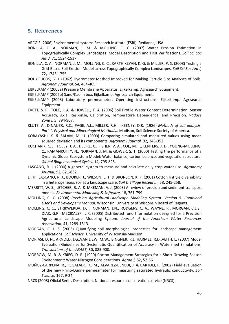
46
5. References ARCGIS (2006) Environmental systems Research Institute (ESRI). Redlands, USA. BONILLA, C. A., NORMAN, J. M. & MOLLING, C. C. (2007) Water Erosion Estimation in
Topographically Complex Landscapes: Model Description and First Verifications. Soil Sci Soc Am J, 71, 1524‐1537.
BONILLA, C. A., NORMAN, J. M., MOLLING, C. C., KARTHIKEYAN, K. G. & MILLER, P. S. (2008) Testing a Grid‐Based Soil Erosion Model across Topographically Complex Landscapes. Soil Sci Soc Am J, 72, 1745‐1755.
BOUYOUCOS, G. J. (1962) Hydrometer Method Improved for Making Particle Size Analyses of Soils. Agronomy Journal, 54, 464‐465.
EIJKELKAMP (2005a) Pressure Membrane Apparatus. Eijkelkamp. Agrisearch Equipment. EIJKELKAMP (2005b) Sand/Kaolin box. Eijkelkamp. Agrisearch Equipment. EIJKELKAMP (2008) Laboratory permeameter. Operating instructions. Eijkelkamp. Agrisearch
Equipment. EVETT, S. R., TOLK, J. A. & HOWELL, T. A. (2006) Soil Profile Water Content Determination: Sensor
Accuracy, Axial Response, Calibration, Temperature Dependence, and Precision. Vadose Zone J, 5, 894‐907.
KLUTE, A., DINAUER, R.C., PAGE, A.L., MILLER, R.H., KEENEY, D.R. (1986) Methods of soil analysis. Part 1. Physical and Mineralogical Methods., Madison, Soil Science Society of America.
KOBAYASHI, K. & SALAM, M. U. (2000) Comparing simulated and measured values using mean squared deviation and its components. Agronomy Journal, 92, 345‐352.
KUCHARIK, C. J., FOLEY, J. A., DELIRE, C., FISHER, V. A., COE, M. T., LENTERS, J. D., YOUNG‐MOLLING, C., RAMANKUTTY, N., NORMAN, J. M. & GOWER, S. T. (2000) Testing the performance of a Dynamic Global Ecosystem Model: Water balance, carbon balance, and vegetation structure. Global Biogeochemical Cycles, 14, 795‐825.
LASCANO, R. J. (2000) A general system to measure and calculate daily crop water use. Agronomy Journal, 92, 821‐832.
LI, H., LASCANO, R. J., BOOKER, J., WILSON, L. T. & BRONSON, K. F. (2001) Cotton lint yield variability in a heterogeneous soil at a landscape scale. Soil & Tillage Research, 58, 245‐258.
MERRITT, W. S., LETCHER, R. A. & JAKEMAN, A. J. (2003) A review of erosion and sediment transport models. Environmental Modelling & Software, 18, 761‐799.
MOLLING, C. C. (2008) Precision Agricultural‐Landscape Modeling System. Version 5. Combined User’s and Developer’s Manual, Wisconsin, University of Wisconsin Board of Regents.
MOLLING, C. C., STRIKWERDA, J.C., NORMAN, J.N., RODGERS, C. A., WAYNE, R., MORGAN, C.L.S., DIAK, G.R., MECIKALSKI, J.R. (2005) Distributed runoff formulation designed for a Precision Agricultural Landscape Modeling System. Journal of the American Water Resources Association, 41, 1289‐1313.
MORGAN, C. L. S. (2003) Quantifying soil morphological properties for landscape management applications. Soil science. University of Wisconsin‐Madison.
MORIASI, D. N., ARNOLD, J.G.,VAN LIEW, M.W., BINGNER, R.L.,HARMEL, R.D.,VEITH, L. (2007) Model Evaluation Guidelines for Systematic Quantification of Accuracy in Watershed Simulations. Transactions of the ASABE, 50, 885‐900.
MORROW, M. R. & KRIEG, D. R. (1990) Cotton Management Strategies for a Short Growing Season Environment: Water‐Nitrogen Considerations. Agron J, 82, 52‐56.
MUÑOZ‐CARPENA, R., REGALADO, C. M., ALVAREZ‐BENEDI, J. & BARTOLI, F. (2002) Field evaluation of the new Philip‐Dunne permeameter for measuring saturated hydraulic conductivity. Soil Science, 167, 9‐24.
NRCS (2008) Oficial Series Description. National resource conservation service (NRCS).

47
RAES, D., STEDUTO, P., HSIAO, T. C. & FERERES, E. (2009) AquaCrop‐‐The FAO Crop Model to Simulate Yield Response to Water: II. Main Algorithms and Software Description. Agron J, 101, 438‐447.
SAVENIJE, H. H. G. (2009) HESS Opinions "The art of hydrology". Hydrology and Earth System Sciences, 13, 157‐161.
SCHAAP, M. G., LEIJ, F. J. & VAN GENUCHTEN, M. T. (2001) Rosetta: a computer program for estimating soil hydraulic parameters with hierarchical pedotransfer functions. Journal of Hydrology, 251, 163‐176.
STROOSNIJDER, L. (2005) Measurement of erosion: Is it possible? CATENA, 64, 162‐173. TOY, T. J., FOSTER, G. R., RENARD, K. G. (2002) Soil erosion: processes, predicition, measurement, and
control, New York, Wiley. VAN GENUCHTEN, M. T. (1980) A Closed‐form Equation for Predicting the Hydraulic Conductivity of
Unsaturated Soils. Soil Sci Soc Am J, 44, 892‐898. VIGIAK, O., DIJCK, S. J. E. V., LOON, E. E. V. & STROOSNIJDER, L. (2006) Matching hydrologic response
to measured effective hydraulic conductivity. Hydrological Processes, 20, 487‐504. ZHU, J., MORGAN, C. L. S., NORMAN, J. M., YUE, W., LOWERY, B. (2004) Combined mapping of soil
properties using a multi‐scale tree‐structured spatial model. Geoderma, 118, 321‐334.

6. Appendix
Table I. Saturated hydraulic conductivity (Ksat) at 0.15 m depth measured and calculated by Rosetta (Schaap et al., 2001)
Location Texture Ksat (cm/day) 20 °C
Ksat (m/s) 20 °C
Ksat (cm/day) Rosetta
Ksat (m/s) Rosetta
1 Sandy Clay Loam 3 3.5·10-7 5.5 6.4·10-7 2 Clay Loam 11 1.3·10-6 7.8 9.0·10-7 3 Sandy Clay Loam 3 3.5·10-7 4.6 5.3·10-7 4 Sandy Clay Loam 0.3 3.5·10-8 3.2 3.7·10-7 5 Sandy Clay Loam 20 2.3·10-6 17.7 2.0·10-6 6 Sandy Clay Loam 12 1.4·10-6 19.6 2.3·10-6 7 Clay Loam 2 2.3·10-7 3.1 3.6·10-7 8 Sandy Clay 32 3.7·10-6 35.3 4.1·10-6 9 Clay Loam 2 2.3·10-7 6.1 7.1·10-7 10 Sandy Clay Loam 5 5.8·10-7 8.8 1.0·10-6 11 Sandy Clay Loam 6 6.9·10-7 7.7 8.9·10-7 12 Sandy Clay Loam 23 2.7·10-6 2.5 2.9·10-7 13 Clay Loam 19 2.2·10-6 15.8 1.8·10-6 14 Sandy Clay Loam 15 1.7·10-6 26.1 3.0·10-6 15 Sandy Clay Loam 11 1.3·10-6 20.4 2.4·10-6 16 Sandy Clay Loam 2 2.3·10-7 5.1 5.9·10-7 17 Sandy Clay Loam 9 1.04·10-6 13.7 1.6·10-6 18 Sandy Clay Loam 11 1.3·10-6 13.8 1.6·10-6
48
I
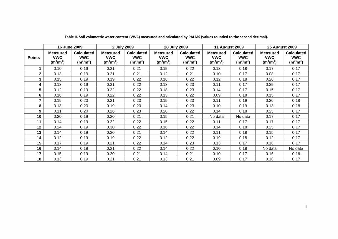
Table II. Soil volumetric water content (VWC) measured and calculated by PALMS (values rounded to the second decimal).
16 June 2009 2 July 2009 28 July 2009 11 August 2009 25 August 2009
Points Measured
VWC (m3/m3)
Calculated VWC
(m3/m3)
Measured VWC
(m3/m3)
Calculated VWC
(m3/m3)
Measured VWC
(m3/m3)
Calculated VWC
(m3/m3)
Measured VWC
(m3/m3)
Calculated VWC
(m3/m3)
Measured VWC
(m3/m3)
Calculated VWC
(m3/m3) 1 0.10 0.19 0.21 0.21 0.15 0.22 0.13 0.18 0.17 0.17 2 0.13 0.19 0.21 0.21 0.12 0.21 0.10 0.17 0.08 0.17 3 0.15 0.19 0.19 0.22 0.16 0.22 0.12 0.18 0.20 0.17 4 0.18 0.19 0.21 0.22 0.18 0.23 0.11 0.17 0.25 0.17 5 0.12 0.19 0.22 0.22 0.18 0.23 0.14 0.17 0.15 0.17 6 0.16 0.19 0.22 0.22 0.13 0.22 0.09 0.18 0.15 0.17 7 0.19 0.20 0.21 0.23 0.15 0.23 0.11 0.19 0.20 0.18 8 0.13 0.20 0.19 0.23 0.14 0.23 0.10 0.19 0.13 0.18 9 0.11 0.20 0.26 0.23 0.20 0.22 0.14 0.18 0.25 0.17
10 0.20 0.19 0.20 0.21 0.15 0.21 No data No data 0.17 0.17 11 0.14 0.19 0.22 0.22 0.15 0.22 0.11 0.17 0.17 0.17 12 0.24 0.19 0.30 0.22 0.16 0.22 0.14 0.18 0.25 0.17 13 0.14 0.19 0.20 0.21 0.14 0.22 0.11 0.18 0.15 0.17 14 0.12 0.19 0.19 0.22 0.12 0.22 0.19 0.18 0.12 0.17 15 0.17 0.19 0.21 0.22 0.14 0.23 0.13 0.17 0.16 0.17 16 0.14 0.19 0.21 0.22 0.14 0.22 0.10 0.18 No data No data 17 0.15 0.19 0.20 0.21 0.14 0.21 0.10 0.17 0.16 0.16 18 0.13 0.19 0.21 0.21 0.13 0.21 0.09 0.17 0.16 0.17
49
II
Top Related