


Languages
Pages
Legal


Universiteit Leiden
Opleiding Informatica
Integrating, Structuring and
Visualising Cancer Data
Name: Wilco Draijer
Date: 17/11/2016
1st supervisor: Katy Wolstencroft2nd supervisor: Fons Verbeek
BACHELOR THESIS
Leiden Institute of Advanced Computer Science (LIACS)
Leiden University
Niels Bohrweg 1
2333 CA Leiden
The Netherlands

Integrating, Structuring andVisualising Cancer Data
Wilco Draijer


Abstract
The primary purpose of this project is to determine what type of database functions better for integration of
cancer data and investigate the added value of visualising cancer data. Data for this research were mostly
collected from COSMIC and the Gene Ontology Consortium. This thesis first describes the set up of a
relational database using MonetDB, followed by the set up of an RDF database, using D2RQ. Secondly the
way of evaluating these databases and the visualisation is described. The visualisation was made using
Gephi. It was concluded that the RDF database is more suitable for the integration of cancer data and the
visualisation did give additional insight. In the future these databases and visualisation can help the mapping
from genes to hallmarks.
i

ii

Acknowledgements
Firstly, I am grateful to God for the insight and wellbeing He has given me during this project. I want
to sincerely thank Katy Wolstencroft, my supervisor, for her continuous expertise and guidance during the
project. I also want to thank Fons Verbeek, my second supervisor, for his additional guidance and the
arrangements he made with regards to a workplace. Lastly, I want to thank Teddy Etoeharnowo, my partner
during the first part of the project, for the pleasant collaboration and his sagacity.
iii

iv

Contents
Abstract i
Acknowledgements iii
1 Introduction 3
1.1 Cancer Data and the Hallmarks of Cancer . . . . . . . . . . . . . . . . . . . . . . . . . . . . . . . . 4
2 Definitions 5
3 Related Work 7
3.1 The Hallmarks of Cancer . . . . . . . . . . . . . . . . . . . . . . . . . . . . . . . . . . . . . . . . . 7
3.2 Bio2RDF . . . . . . . . . . . . . . . . . . . . . . . . . . . . . . . . . . . . . . . . . . . . . . . . . . . 7
3.3 Relational database vs RDF . . . . . . . . . . . . . . . . . . . . . . . . . . . . . . . . . . . . . . . . 8
4 Methods and Development 10
4.1 The Relational Database . . . . . . . . . . . . . . . . . . . . . . . . . . . . . . . . . . . . . . . . . . 10
4.1.1 Data Cleaning . . . . . . . . . . . . . . . . . . . . . . . . . . . . . . . . . . . . . . . . . . . . 12
4.1.2 Provenance . . . . . . . . . . . . . . . . . . . . . . . . . . . . . . . . . . . . . . . . . . . . . 12
4.1.3 Evaluation . . . . . . . . . . . . . . . . . . . . . . . . . . . . . . . . . . . . . . . . . . . . . . 12
4.2 The RDF Database . . . . . . . . . . . . . . . . . . . . . . . . . . . . . . . . . . . . . . . . . . . . . 12
4.2.1 URI’s . . . . . . . . . . . . . . . . . . . . . . . . . . . . . . . . . . . . . . . . . . . . . . . . . 13
4.2.2 Evaluation . . . . . . . . . . . . . . . . . . . . . . . . . . . . . . . . . . . . . . . . . . . . . . 13
4.3 The Visualisation . . . . . . . . . . . . . . . . . . . . . . . . . . . . . . . . . . . . . . . . . . . . . . 13
4.3.1 Gephi . . . . . . . . . . . . . . . . . . . . . . . . . . . . . . . . . . . . . . . . . . . . . . . . . 15
5 Results and Evaluation 18
5.1 Relational Database . . . . . . . . . . . . . . . . . . . . . . . . . . . . . . . . . . . . . . . . . . . . . 18
5.2 RDF . . . . . . . . . . . . . . . . . . . . . . . . . . . . . . . . . . . . . . . . . . . . . . . . . . . . . . 18
5.3 Visualisation . . . . . . . . . . . . . . . . . . . . . . . . . . . . . . . . . . . . . . . . . . . . . . . . . 19
v

5.3.1 Cellular Component . . . . . . . . . . . . . . . . . . . . . . . . . . . . . . . . . . . . . . . . 19
5.3.2 Molecular Function . . . . . . . . . . . . . . . . . . . . . . . . . . . . . . . . . . . . . . . . . 20
5.3.3 Biological Process . . . . . . . . . . . . . . . . . . . . . . . . . . . . . . . . . . . . . . . . . . 20
6 Conclusions 23
6.1 Future work . . . . . . . . . . . . . . . . . . . . . . . . . . . . . . . . . . . . . . . . . . . . . . . . . 23
6.1.1 Cellular Component . . . . . . . . . . . . . . . . . . . . . . . . . . . . . . . . . . . . . . . . 24
6.1.2 Molecular Function . . . . . . . . . . . . . . . . . . . . . . . . . . . . . . . . . . . . . . . . . 24
6.1.3 Biological Process . . . . . . . . . . . . . . . . . . . . . . . . . . . . . . . . . . . . . . . . . . 25
Bibliography 25
vi

List of Tables
5.1 Evaluation questions . . . . . . . . . . . . . . . . . . . . . . . . . . . . . . . . . . . . . . . . . . . . 19
1
List of Figures
3.1 Hallmarks of cancer . . . . . . . . . . . . . . . . . . . . . . . . . . . . . . . . . . . . . . . . . . . . 8
4.1 ER-diagram for the relational database . . . . . . . . . . . . . . . . . . . . . . . . . . . . . . . . . 11
4.2 Heatmap of Biological Process . . . . . . . . . . . . . . . . . . . . . . . . . . . . . . . . . . . . . . 15
4.3 Before executing the Force Atlas 2 algorithm . . . . . . . . . . . . . . . . . . . . . . . . . . . . . . 16
4.4 After executing the Force Atlas 2 algorithm . . . . . . . . . . . . . . . . . . . . . . . . . . . . . . . 16
4.5 Screenshot of Gephi . . . . . . . . . . . . . . . . . . . . . . . . . . . . . . . . . . . . . . . . . . . . 17
5.1 All genes and GO terms classified under Cellular Component (out–degree) . . . . . . . . . . . . 20
5.2 All genes and GO terms classified under Molecular Function (out–degree) . . . . . . . . . . . . 21
5.3 All genes and GO terms classified under Biological Process (out–degree) . . . . . . . . . . . . . 22
6.1 All genes and GO terms classified under Cellular Component (in–degree) . . . . . . . . . . . . . 24
6.2 All genes and GO terms classified under Molecular Function (in–degree) . . . . . . . . . . . . . 25
6.3 All genes and GO terms classified under Biological Process (in–degree) . . . . . . . . . . . . . . 26
2

Chapter 1
Introduction
Cancer is a leading cause of death with 8.2 million cancer-related deaths in 2012 [1] and is therefore a focus
for large-scale research efforts. A lot of the data from all this research is publicly available. Databases about
cancer, like COSMIC (a curated set of gene mutations) [2], and general biology databases, like Reactome (a
curated and peer reviewed pathway database) [3], KEGG (a pathway database focussing on molecular inter-
actions, reactions and relations) [4] and Gene Ontology Consortium (gene product description database) [5],
are a few examples of the databases storing this data used for this research. This data is not only interesting
from a biological point of view, but also from a data science point. Cancer data can have many different
forms. Functional descriptors, pathways and mutations are only a few examples. This heterogeneous data is
also dynamic, since it is continuously updated. Integrating and cataloguing this data can lead to new insights
into cancer genes. It can expose implicit relationships between the data from all the different sources. This is
why it is important to create a system which can integrate new data and merge it with the data the system
contains. The traditional way of doing this is to create a relational database. This is not always a suitable way,
since an SQL Database schema can’t be easily changed when new data arrives and an SQL database can’t
query other datasources without integrating that data or postprocessing. A Resource Description Framework
(RDF) [6] database on the other hand is more dynamic since it can change a schema relatively easily and it
is possible to query other datasources without integrating the data. We will compare these two databases
to see which of the two is more suitable. The Gene Ontology terms are concepts or classes to describe gene
functions. All these terms are organised in a hierarchical structure, since they have super– and subclass terms
that are respectively less or more specific concepts or classes. When this hierarchy is visualised, it is easier
understood and can also give more or new insights. Whereas the hierarchical structure can be hidden when
it is shown in a relational representation.
3
4 Chapter 1. Introduction
1.1 Cancer Data and the Hallmarks of Cancer
Cancer hallmarks are underlying principles covering all aspects and functions of cancer. The overall goal
is to create a more concrete mapping from genes to these hallmarks using gene ontology term annotation.
The hallmarks framework is a useful conceptual framework, but it is interpreted in different ways in different
studies. When a more systematic mapping is created between data and hallmarks, there will be less ambiguity
in the interpretation. To reach this goal we created a subgoal for this project, namely finding out what type
of database is better in connecting the different datasources, relational or RDF, and visualising cancer genes
with the related gene ontology terms in the gene hierarchy. This is done following the research question:
How does semantic modelling contribute to the data model and clustering of cancer data?
This thesis describes two parts. The first part describes the creation of a relational database containing data
from different sources. This is done in collaboration with Teddy Etoeharnowo, student at Leiden University.
The second part describes creating an RDF database, linking it to other databases and visualising the data,
which I did on my own. The clustering of the data mentioned in the research question is done by Teddy
and described in his thesis. First we will take a look at the databases used in this project and how RDF
works. Next we explain the hallmarks of cancer, the differences between RDF and relational databases and
how the differences with RDF could be exploited when studying the hallmarks of cancer. Then we discuss
the platform we set up to connect all the different sources. We evaluate our contributions and lastly we will
draw our conclusion.

Chapter 2
Definitions
In this chapter we will elucidate the different sources and the Research Description Framework.
We retrieved data for our project from the following sources:
• The ’Catalogue of somatic mutations in cancer’ (COSMIC) [2] contains a curated set of gene mutations
involved in cancer and is used as a gold standard data set for this project.
• Reactome ”is a free, open-source, curated and peer reviewed pathway database.” [3]
• Kyoto Encyclopedia of Genes and Genomes (KEGG) Pathways wires ”diagrams of molecular interac-
tions, reactions, and relations.” [4]
• Gene Ontology (GO) [5] contains descriptions for gene products across databases in terms of three
different aspects.
The GO database classifies functions along three aspects:
• Molecular Function
• Cellular Component
• Biological Process
These three aspects mark the top of the GO hierarchy. An ontology is a definition of an entity and their
properties and relations in a certain domain [7]. A gene ontology does this for genes in an hierarchical
structure.
A Relational Database [8] holds a lot of data organised in tables. This data can be accessed, defined, con-
trolled and manipulated using Structured Query Language (SQL) [9]. A relational database is the standard
database to store a lot of data.
5

6 Chapter 2. Definitions
MonetDB is a database management system used to set up relational databases [10].
Resource Description Framework (RDF) [6] is the W3C standard for the semantic web to interchange data
on the web. RDF uses Uniform Resource Identifiers (URI’s), these are strings of characters to identify sources
or relations, to denote a resource and uses them in triples (RDF statements) to link two URI’s together. A
triple exists of a subject (a URI), a predicate (a relation/link/URI) and a object (a URI or a literal). When
all this data is linked together it forms a graph, where the nodes are the URI’s and the edges the relations
between them. When data is structured in this way, either on the web or on a local database, it can be queried
using SPARQL [11]. SPARQL stands for SPARQL Protocol and RDF Query Language and it works similar to
SQL. To query a data on the web, that database should have a SPARQL endpoint. This is the link used in a
federated query.
Provenance [12], in the data science field, means where the data comes from and when it was retrieved.
This allows more verification when checking the data, since it could have multiple sources or be verified at
multiple times. It can also help with conflicting data to find the source of the conflict.
Chapter 3
Related Work
In this section we will describe the hallmarks of cancer and list the advantages RDF has over a relational
database.
3.1 The Hallmarks of Cancer
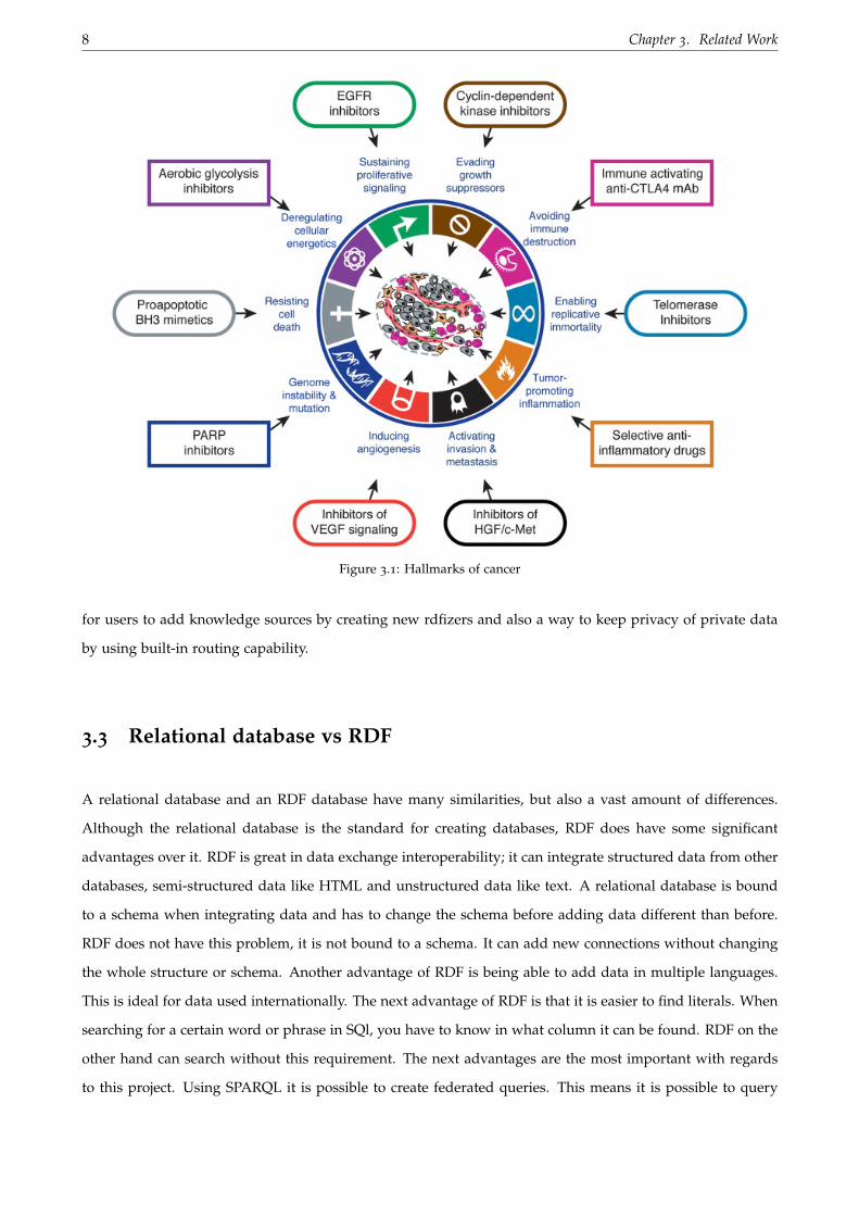
The hallmarks of cancer are conceptual descriptions of the disruptive cellular processes that occur in the
development of cancer. Cancer has eight hallmarks and two enabling characteristics as shown in figure 3.1.
These hallmarks include sustaining proliferative signalling, evading growth suppressors, avoiding immune
destruction, enabling replicative immortality, activating invasion and metastasis, inducing angiogenesis and
resisting cell death. The enabling characteristics are genome instability and mutation, and tumor-promoting
inflammation. Besides the cancer cells, tumours contain normal cells that also contribute to the hallmarks.
Understanding and recognising these hallmarks will significantly help treat human cancer [13]. There have
been many attempts to map cancer hallmarks to functional data, but no systematic method for identifying
hallmarks has been established. This means the mappings are heterogeneous and incomparable.
3.2 Bio2RDF
Bio2RDF [14] is a mashup system to help the process of bioinformatics knowledge integration. More than
twenty different public bioinformatics data sources are available in a normalised RDF format from the
Bio2RDF.org server. With the use of three different rdfizer (converters to RDF) Bio2RDF locally stored multi-
ple databases, related to specific topics, so these can be extracted in minutes rather than hours. The Bio2RDF
framework provides access to normalised RDF documents from many different sources, and offers a method
7
8 Chapter 3. Related Work
Figure 3.1: Hallmarks of cancer
for users to add knowledge sources by creating new rdfizers and also a way to keep privacy of private data
by using built-in routing capability.
3.3 Relational database vs RDF
A relational database and an RDF database have many similarities, but also a vast amount of differences.
Although the relational database is the standard for creating databases, RDF does have some significant
advantages over it. RDF is great in data exchange interoperability; it can integrate structured data from other
databases, semi-structured data like HTML and unstructured data like text. A relational database is bound
to a schema when integrating data and has to change the schema before adding data different than before.
RDF does not have this problem, it is not bound to a schema. It can add new connections without changing
the whole structure or schema. Another advantage of RDF is being able to add data in multiple languages.
This is ideal for data used internationally. The next advantage of RDF is that it is easier to find literals. When
searching for a certain word or phrase in SQl, you have to know in what column it can be found. RDF on the
other hand can search without this requirement. The next advantages are the most important with regards
to this project. Using SPARQL it is possible to create federated queries. This means it is possible to query

3.3. Relational database vs RDF 9
external databases with our data, without having to download all the data on your system or server. RDF is
also better at handling hierarchical structured data. This should make querying the GO database and other
ontology data easier than it would be using SQL. The last advantage RDF has is the fact that it is a graph.
This makes it easier to visualise the data. When visualising a relational database it will show tables, whereas
visualising RDF can create a big graph, not only showing all the relations between URI’s, but also hierarchical
structures using directed edges.
These last three advantages (federated querying, handling hierarchical structure and visualising the data)
create great expectations for our project, since we use a lot of different sources, query hierarchical data and
want to visualise it. To see if the results will live up to the expectations, we will test the RDF and relational
database both using Jim Gray’s ”20 questions” method [15]. The idea is to ask the 20 most important questions
(queries in this case) to test your system. We used this method to compare the relational database with the
RDF one.

Chapter 4
Methods and Development
In this chapter will be explained how the relational database was set up, what problems came up, the way
provenance was recorded, how the RDF database was set up and finally how the data was visualised.
4.1 The Relational Database
To set up the relational database we created an ER-diagram and database using MonetDB [10]. MonetDB was
the preferred choice since the some of the developers were present at Leiden University, so when encountering
problems we could ask them for help. Another advantage MonetDB has, is the embedded version for R. This
is very useful for the data mining the collected data. We started off with getting the data from the COSMIC
gene census [16]. This gene census is a curated list of all genes that have mutations proven to be associated
with cancer and is a gold standard set. It contained the following data for all genes, the datatype is shown in
parentheses:
• Gene Symbol (String)
• Name (String)
• Entrez ID (Integer)
• Genome Location (String)
• Chromosome band (String)
• Somatic Tumour Type (String)
• Germline Tumour type (String)
10

4.1. The Relational Database 11
• Tissue Type (Character)
• Molecular Genetics (String)
• Mutation Types (String)
• Synonyms (String)
All this data was formatted as a Comma-separated Values file (CSV). We split all these columns and linked
it all to the Entrez ID (a unique number bound to a single gene). This gave a lot of weak entities in the
ER-diagram, meaning this data could not be uniquely identified by the attributes (i.e. multiple rows could
have the same value), but only by its Entrez ID. This means all the data was split into multiple CSV files,
where Entrez ID was almost always the first column (and therefore the key). After creating the diagram and
adding all the data to the database, we did the same for KEGG, Gene Ontology and Reactome. Figure 4.1
shows the ER-diagram. It shows that the only attribute that did not need Entrez ID as a foreign key is the
KEGG Human ID. This is because this ID also uniquely identifies to a gene.
Figure 4.1: ER-diagram for the relational database
In figure 4.1 the blue relations come from COSMIC, the red from the Gene Ontology, all yellow from Kegg
and the green from Reactome. The purple relation is a combination between COSMIC and Gene Ontology
since we got synonyms from both of these sources.

12 Chapter 4. Methods and Development
4.1.1 Data Cleaning
To add all the data to the database we created csv-files containing all the data. This type of files split the data
into different columns depending on a chosen delimiter. This gave a minor setback when discovering that
the prefered delimiters, comma, semicolon and colon, were also used in the data. This meant that the data
would split into multiple columns when this was not supposed to. To solve this we replaced the semicolon
in the data with a comma and chose the semicolon as the delimiter.
4.1.2 Provenance
After adding all this data in the different tables and creating different entities in the diagram, we did the
same thing for the provenance of all the data. Provenance is important with dynamic data from multiple
sources. When data from different sources or timestamps conflicts with each other, it is important to know
which source and which update is the source of the conflict. It is furthermore good for the verification of
the data. If the same data comes from multiple sources, consensus may show and will therefore be more
reliable. We created a table specially for the provenance listing all the tables that got their data from a certain
database. The exception to this was the synonyms table. Since the synonyms came from COSMIC and KEGG
we added a column to this table listing whether it came from COSMIC or KEGG.
4.1.3 Evaluation
To evaluate the relational database, we queried the relational database using the top 18 questions identified by
potential database users (in this case, bioinformaticians researching cancer data), using the method mentioned
in section 3.3 [15]. We checked if not only we could create the queries and run them, but also if the answers
to the queries were correct by sampling.
4.2 The RDF Database
To query our relational database with existing databases there should either be a local copy of the database
or post-processing should be done. This takes up extra space and time for every new database we want to
query, but not integrate in the existing database. A Resource Description Framework (RDF) database has the
advantage of being able to query existing and online databases without having to get a local copy; the data
is queried at its source. The RDF database could be set up in two ways. The first is setting it up from scratch
like the relational database. The second one is converting the relational database. Since I had no knowledge
of RDF at the start of the project and it would take significantly less time, I decided to go with the second
4.3. The Visualisation 13
option. The D2RQ-tool was seemingly ideal for this since “the D2RQ Platform is a system for accessing
relational databases as virtual, read-only RDF graphs. It offers RDF-based access to the content of relational
databases without having to replicate it into an RDF store.” [17] Converting the database was relatively easy.
After downloading a JDBC driver from the MonetDB site, the relational database could be mapped to an
RDF one. We had to create a mapping using the generator D2RQ provided. This generator created the entire
RDF graph mapped from the relational database. There was one issue with the mapping with regards to the
level of the column names. The column names had the following format databasename.tablename.columnname.
Unfortunately third level column names (names that exist out of three parts) were not supported. The
solution to this was to create aliases for the database name and table name, so the format would change
into databasenametablename.columnname. With the renewed mapping we could run the RDF database. After
the set-up we found out federated querying was not supported in this version of D2RQ (though it was the
newest on their website). Since this is one of the main benefits from RDF over relational databases this was
important to be fixed. Luckily it was mentioned as an issue on GitHub, where the solution could be found,
namely a small change in the source code.
4.2.1 URI’s
One of the advantages of RDF was that it was possible to link the data from GO directly to URI’s from
Bio2RDF [14]. ”Bio2RDF is an open-source project that uses Semantic Web technologies to build and provide
the largest network of Linked Data for the Life Sciences.” [18] It has a SPARQL endpoint to query the entire
database. This was very useful, since the GO terms in our data were single terms, but did not have the
hierarchical structure and data Bio2RDF does have. This meant that when changing the single GO terms in
our database to the URI used by Bio2RDF, the data was part of the entire hierarchy and was automatically
updated. It also meant that querying the data sources is easier. It is still necessary to make the query
federated, but it needs one less sub-query this way. With the URI’s in place, it was possible to make efficient
queries using SPARQL [11].
4.2.2 Evaluation
To evaluate the RDF database we used the same 14 questions mentioned in subsection 4.1.3.
4.3 The Visualisation
When looking at data in a tabular or listed format it is very hard to uncover relationships between genes
and/or GO terms. When the data is visualised, it is easier to uncover implicit relationships. Since RDF could
14 Chapter 4. Methods and Development
query multiple sources, it was relatively easy to translate the data from these sources with our data to a visual
graph. Using directed edges it was also possible to visualise the hierarchical structure from the GO database.
For the visualisation Gephi was a good choice. Gephi is an ”interactive visualisation and exploration platform
for all kinds of networks and complex systems, dynamic and hierarchical graphs.” [19] Gephi has multiple
plug-ins, algorithms and functions to manipulate the graph available.
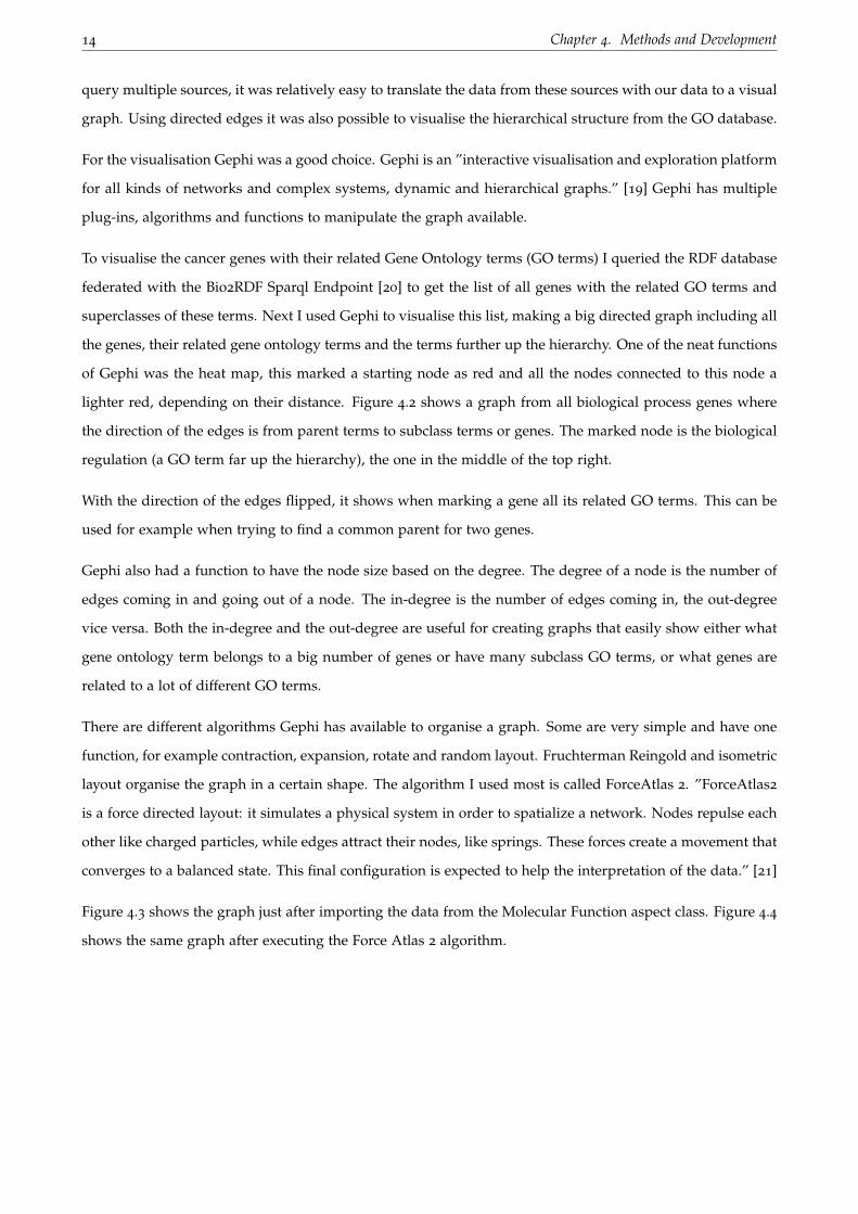
To visualise the cancer genes with their related Gene Ontology terms (GO terms) I queried the RDF database
federated with the Bio2RDF Sparql Endpoint [20] to get the list of all genes with the related GO terms and
superclasses of these terms. Next I used Gephi to visualise this list, making a big directed graph including all
the genes, their related gene ontology terms and the terms further up the hierarchy. One of the neat functions
of Gephi was the heat map, this marked a starting node as red and all the nodes connected to this node a
lighter red, depending on their distance. Figure 4.2 shows a graph from all biological process genes where
the direction of the edges is from parent terms to subclass terms or genes. The marked node is the biological
regulation (a GO term far up the hierarchy), the one in the middle of the top right.
With the direction of the edges flipped, it shows when marking a gene all its related GO terms. This can be
used for example when trying to find a common parent for two genes.
Gephi also had a function to have the node size based on the degree. The degree of a node is the number of
edges coming in and going out of a node. The in-degree is the number of edges coming in, the out-degree
vice versa. Both the in-degree and the out-degree are useful for creating graphs that easily show either what
gene ontology term belongs to a big number of genes or have many subclass GO terms, or what genes are
related to a lot of different GO terms.
There are different algorithms Gephi has available to organise a graph. Some are very simple and have one
function, for example contraction, expansion, rotate and random layout. Fruchterman Reingold and isometric
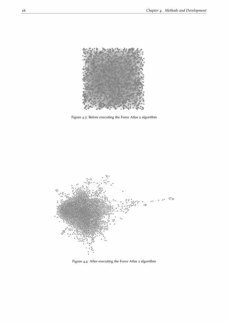
layout organise the graph in a certain shape. The algorithm I used most is called ForceAtlas 2. ”ForceAtlas2
is a force directed layout: it simulates a physical system in order to spatialize a network. Nodes repulse each
other like charged particles, while edges attract their nodes, like springs. These forces create a movement that
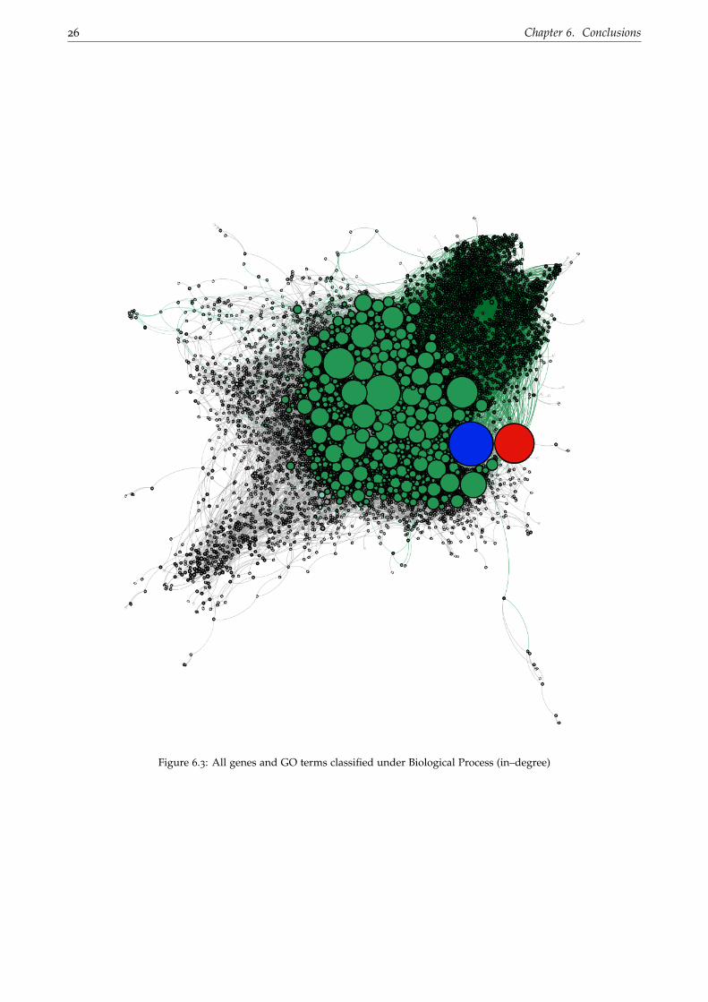
converges to a balanced state. This final configuration is expected to help the interpretation of the data.” [21]
Figure 4.3 shows the graph just after importing the data from the Molecular Function aspect class. Figure 4.4
shows the same graph after executing the Force Atlas 2 algorithm.

4.3. The Visualisation 15
Figure 4.2: Heatmap of Biological Process
4.3.1 Gephi
In figure 4.5 is a screenshot of the program shown. At the top left are three tabs shown, ”Overview” is for
editing the graph structure, ”Data Laboratory” is for editing the data and ”Preview” is for editing the graph
in a visual manner. Below the tabs is a part for the appearance, I used this mainly to base the node size on the
out-degree. Below the appearance is the algorithm part, where you can select, edit and run an algorithm to
edit the graph. Just left of the graph is a toolbar with multiple functions, the orange sun like symbol (selected
in the figure) is the heat map. On the right is a part for statistics, I used this mainly to calculate the degree
for every node. When the ”Average Degree” has run once, the Data Laboratory shows both the in-degree and
the out-degree for every node.
16 Chapter 4. Methods and Development
Figure 4.3: Before executing the Force Atlas 2 algorithm
Figure 4.4: After executing the Force Atlas 2 algorithm

4.3. The Visualisation 17
Figure 4.5: Screenshot of Gephi

Chapter 5
Results and Evaluation
In this chapter, we describe the evaluation of the relational and RDF database, and the visualisation.
5.1 Relational Database
As mentioned before, to evaluate the relational database the ”20 questions” method from Jim Gray was
used [15]. Instead of 20 questions we queried 18, because additional questions did not add value to the
evaluation. The 18 questions we tested were the following:
SQL does not support federated querying. This made questions 8, 10 and 18 unable to be answered. Ques-
tions 6, 14 to 17 could not be fully answered; it only gave the GO terms we had in our database. All these
questions could be answered with post-processing or downloading a local copy of the external database (GO
in this case).
5.2 RDF
To evaluate the RDF database the same questions were used as in section 5.1. Using federated querying
it was possible to also answer the questions using external data sources. These questions also showed a
new problem. D2RQ did not support the combination of the aggregates HAVING and COUNT. This made
5 questions left unanswered, since it did need the combination of the two, namely 5, and 7 to 11. Note that
these questions probably could be answered if the system was not made with D2RQ, but with another tool.
18

5.3. Visualisation 19
Table 5.1: Evaluation questions
Question Relational RDF1. Return all the pathways associated with gene X X X2. What other genes from COSMIC are involved in these path-
ways?X X
3. Return all the cancer genes with recessive mutations X X4. Which are oncogenes and which are tumour suppressor genes? X X5. Return all the cancer genes that are associated with more than
one cancer - which cancers, which tissue types?X 7
6. Which pathways and Gene Ontology terms are associated withbreast cancer?
~ X
7. Which Gene Ontology Biological Process terms are common toall melanomas - or are there none common to all?
X 7
8. Are there any shared GO terms further up the hierarchy? 7 7
9. Which GO Molecular function terms are common to allmelanomas?
X 7
10. Are there any shared GO terms further up the hierarchy? 7 7
11. Which GO Cellular Component terms are common to allmelanomas?
X 7
12. Return all the genes that are not assigned to any pathways X X13. Return all the genes that are only assigned to pathways from
Reactome, but not from KEGGX X
14. Which GO biological process terms are associated with thecytokine-cytokine receptor interaction pathway?
~ X
15. Which genes are associated with angiogenesis? ~ X16. Which genes are associated with apoptosis? ~ X17. Which genes are associated with signalling and binding? ~ X18. Which genes are in the same cellular components? 7 X
5.3 Visualisation
The visualisation was evaluated by creating graphs for all three aspect classes (Cellular Component, Molecu-
lar Function and Biological Process) and examined for nodes or connections that stood out. It allowed us to
map the flat gene mutation data onto the hierarchical structure of the gene ontology, revealing new ways of
exploring the functional relationships between gene mutations.
5.3.1 Cellular Component
Figure 5.1 shows the genes and related GO terms of cellular component. The node size is based on the
out-degree. The red node is the GO term furthest up the hierarchy, cellular component. The four biggest
nodes (and therefore the GO terms with the most connected genes) are nucleus, nucleoplasm, cytoplasm and
cytosol. These nodes and their neighbours are marked with pink, yellow, cyan and blue respectively. The
genes that relate to more than one of these GO terms have the colours of its parents mixed.

20 Chapter 5. Results and Evaluation
Figure 5.1: All genes and GO terms classified under Cellular Component (out–degree)
5.3.2 Molecular Function
Figure 5.2 shows the genes and related GO terms of molecular function. The node size is based on the
out-degree. The red node is the GO term furthest up the hierarchy, molecular function. The biggest node is
protein binding and is marked with cyan.
5.3.3 Biological Process
Figure 5.3 shows the genes and related GO terms of biological process. The node size is based on the out-
degree. The red node is the GO term furthest up the hierarchy, biological process. The biggest node is
biological regulation and is marked with cyan. As cancer is about disrupting existing regulatory processes
in the cell, this was not surprising. The graph additionally shows how clusters of genes were associated
with particular forms of disruption and therefore provides cancer specialists with a new way of examining
similarities and differences between these clusters.

5.3. Visualisation 21
Figure 5.2: All genes and GO terms classified under Molecular Function (out–degree)

22 Chapter 5. Results and Evaluation
Figure 5.3: All genes and GO terms classified under Biological Process (out–degree)

Chapter 6
Conclusions
The comparison between a relational database and an RDF one results in a reasonable preference for RDF.
The flexibility RDF brings is a big advantage when dealing with multiple sources. The fact that it is possible
to query different sparql endpoints and retrieving data that way costs less time and space as opposed to
making a local copy of every database or post-process the result of the queries. It also gives an advantage for
visualisation since it is easier to query hierarchical structures. The relational and RDF database do perform
similarly well, apart from the hierarchical data and for federating with other resources.
The visualisation of the three aspects revealed multiple things that could be overlooked watching only the
textual data. Gephi allows the visualisation of functional clusters in the data. The function to base the node
size on the out-degree is also ideal to quickly notice the important GO terms.
6.1 Future work
The overall goal of this project is to link genes to hallmarks. The database and visualisation made in this
project could help that research. The visualisations made in this project were focused on the Gene Ontology
terms, not on the genes. After linking a lot of genes to Hallmarks, the focus will shift towards which genes
play the most important role in cancer. When the node size in my visualisation is based on the in-degree it
is easy to see which genes are related to the most GO terms and could therefor be important in cancer. The
in-degree results can also be compared with the biological pathway data already in the database, to identify
which pathways are key and pivotal for different clusters of cancer types. I created three examples of these
visualisations, one for each aspect class.
23

24 Chapter 6. Conclusions
6.1.1 Cellular Component
In figure 6.1 is the colouring done the same as in 5.1 The two biggest nodes (the genes with the most amount
of related GO terms) are ”ezrin” and ”catenin (cadherin-associated protein), beta 1”, marked as red and green
respectively.
Figure 6.1: All genes and GO terms classified under Cellular Component (in–degree)
6.1.2 Molecular Function
In figure 6.2 is the heat mapped node ”protein binding”. The two biggest nodes are ”tumor protein p53” and
”retinoic acid receptor, alpha”, marked as blue and green respectively.

6.1. Future work 25
Figure 6.2: All genes and GO terms classified under Molecular Function (in–degree)
6.1.3 Biological Process
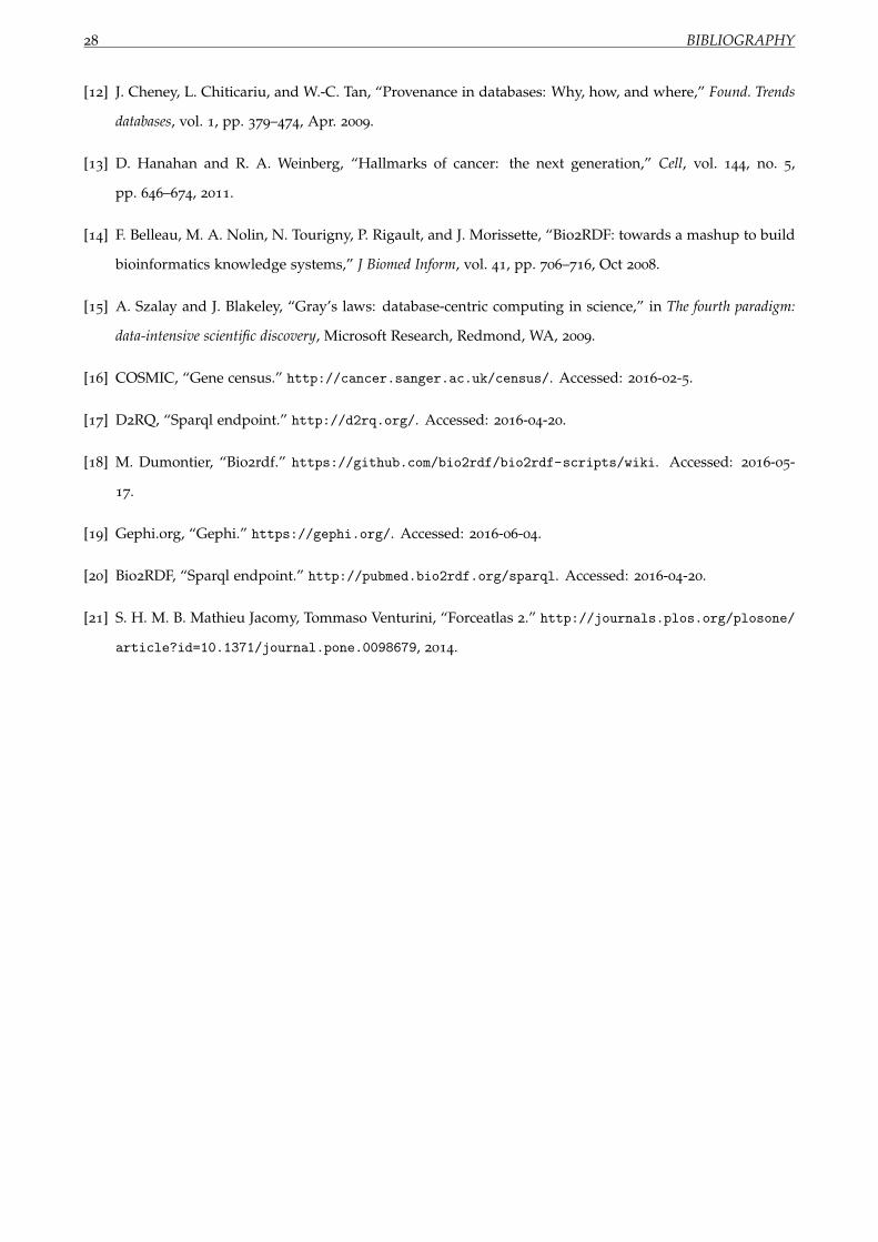
In figure 6.3 is the heat mapped node (with a green palette) ”biological regulation”. The two biggest nodes
are ”tumor protein p53” and ”Notch homolog 1, translocation-associated (Drosophila) (TAN1)”, marked as
blue and red respectively. p53 came our highest in both Biological Process and Molecular Function - this is
very significant. P53 plays a key role in binding and regulation and has already been shown to be associated
with many different cancers. This also suggests a role in multiple hallmark processes, which can be validated
by combining the results of this work with the results of a related project by Atagun Isiktas, an Erasmus
exchange student.
26 Chapter 6. Conclusions
Figure 6.3: All genes and GO terms classified under Biological Process (in–degree)
Bibliography
[1] I. A. for Research on Cancer, “Fact sheet on cancer.” http://globocan.iarc.fr/Pages/fact_sheets_
cancer.aspx. Accessed: 2016-05-20.
[2] S. A. Forbes, G. Bhamra, S. Bamford, E. Dawson, C. Kok, J. Clements, A. Menzies, J. W. Teague, P. A.
Futreal, and M. R. Stratton, “The Catalogue of Somatic Mutations in Cancer (COSMIC),” Curr Protoc
Hum Genet, vol. Chapter 10, p. Unit 10.11, Apr 2008.
[3] P. D’Eustachio, “Reactome knowledgebase of human biological pathways and processes,” Methods Mol.
Biol., vol. 694, pp. 49–61, 2011.
[4] M. Kanehisa and S. Goto, “KEGG: kyoto encyclopedia of genes and genomes,” Nucleic Acids Res., vol. 28,
pp. 27–30, Jan 2000.
[5] M. Ashburner, C. A. Ball, J. A. Blake, D. Botstein, H. Butler, J. M. Cherry, A. P. Davis, K. Dolinski, S. S.
Dwight, J. T. Eppig, M. A. Harris, D. P. Hill, L. Issel-Tarver, A. Kasarskis, S. Lewis, J. C. Matese, J. E.
Richardson, M. Ringwald, G. M. Rubin, and G. Sherlock, “Gene ontology: tool for the unification of
biology. The Gene Ontology Consortium,” Nat. Genet., vol. 25, pp. 25–29, May 2000.
[6] W3C, “Resource description framework.” https://www.w3.org/RDF/. Accessed: 2016-04-20.
[7] A. F.-E. F. Arvidsson, “Ontology.” http://www.ida.liu.se/~janma56/SemWeb/. Accessed: 2016-08-17.
[8] M. Rouse, “Relational database.” http://searchsqlserver.techtarget.com/definition/
relational-database. Accessed: 2016-08-17.
[9] W3C, “Structured query language.” http://www.w3schools.com/sql/. Accessed: 2016-08-17.
[10] MonetDB, “Monetdb.” https://www.monetdb.org/. Accessed: 2016-02-05.
[11] S. A. Prud’hommeaux E, “Sparql query language for rdf.” http://www.w3.org/TR/rdf-sparql-query/.
Accessed: 2016-04-15.
27
28 BIBLIOGRAPHY
[12] J. Cheney, L. Chiticariu, and W.-C. Tan, “Provenance in databases: Why, how, and where,” Found. Trends
databases, vol. 1, pp. 379–474, Apr. 2009.
[13] D. Hanahan and R. A. Weinberg, “Hallmarks of cancer: the next generation,” Cell, vol. 144, no. 5,
pp. 646–674, 2011.
[14] F. Belleau, M. A. Nolin, N. Tourigny, P. Rigault, and J. Morissette, “Bio2RDF: towards a mashup to build
bioinformatics knowledge systems,” J Biomed Inform, vol. 41, pp. 706–716, Oct 2008.
[15] A. Szalay and J. Blakeley, “Gray’s laws: database-centric computing in science,” in The fourth paradigm:
data-intensive scientific discovery, Microsoft Research, Redmond, WA, 2009.
[16] COSMIC, “Gene census.” http://cancer.sanger.ac.uk/census/. Accessed: 2016-02-5.
[17] D2RQ, “Sparql endpoint.” http://d2rq.org/. Accessed: 2016-04-20.
[18] M. Dumontier, “Bio2rdf.” https://github.com/bio2rdf/bio2rdf-scripts/wiki. Accessed: 2016-05-
17.
[19] Gephi.org, “Gephi.” https://gephi.org/. Accessed: 2016-06-04.
[20] Bio2RDF, “Sparql endpoint.” http://pubmed.bio2rdf.org/sparql. Accessed: 2016-04-20.
[21] S. H. M. B. Mathieu Jacomy, Tommaso Venturini, “Forceatlas 2.” http://journals.plos.org/plosone/
article?id=10.1371/journal.pone.0098679, 2014.
Top Related