


Languages
Pages
Legal


ECN-C--05-066
Uncertainties in Cup Anemometer Calibrations
Type A and Type B uncertainties P.J. Eecen
M. de Noord
JUNE 2005

Acknowledgement/Preface The work described in this report is carried out within the framework of the European ACCUWIND research project under contract with the European Commission. CE Contract Number: NNE5-2001-00831 ECN Project number: 7.4342 DEWI provided information on their wind tunnel for the type B uncertainty assessment. Frank Ormel and Erik Korterink have performed the measurements in the DNW wind tunnel in 2003 (Chapter 3.6). Abstract ECN Wind Energy is accredited according ISO 17025 to perform power performance measure-ments of wind turbines following IEC 61400-12 and Measnet. The typical results of these measurements are measured power curves of the wind turbines. These curves show the electrical power versus the wind speed. Part of the power performance analysis is the uncertainty analysis. In power performance measurements according IEC 61400-12 or Measnet, the wind speed is measured using cup anemometers. The uncertainty of the wind speed measurements depends among others on the calibration uncertainty. The cup-anemometer calibration uncertainty is divided in Type A and Type B uncertainty. The Type A uncertainty is the statistical uncertainty of the wind speed measurement and can be calculated from the wind speed measurements. The Type B uncertainty includes all uncertainties that do not have a statistical background. For example, these are uncertainties due to temperature changes, air pressure changes, transducer gain influences, and digital conversion influences, etcetera. This document presents an overview of the type B uncertainties of a cup anemometer calibration following the Measnet Cup Anemometer Calibration Procedure, Version 1, September 1997 and the proposal for the IEC 61400-12 that is currently under vote. For the calculations, the numbers applying to the DEWI wind tunnel are used throughout the report. It is shown that the cup anemometer in wind tunnels has unstable behaviour due to the turbulent wakes of the cups. An analysis of uncertainties due to regression in cup anemometer calibrations is presented and compared to the standard uncertainty.
2 ECN-C--05-066

Contents
List of tables 5 List of figures 5 1. Introduction 7 2. CUP ANEMOMETER CALIBRATION UNCERTAINTY 9
2.1 Introduction 9 2.1.1 Wind tunnel correction MEASNET 10 2.1.2 Wind tunnel correction DEWI 11 2.1.3 Wind tunnel calibration MEASNET 12 2.1.4 Wind tunnel calibration DEWI 13 2.1.5 Pressure transducer sensitivity MEASNET 14 2.1.6 Pressure transducer sensitivity DEWI 15 2.1.7 Pressure transducer signal conditioning gain MEASNET 16 2.1.8 Pressure transducer signal conditioning gain DEWI 17 2.1.9 Pressure transducer data sampling conversion MEASNET 18 2.1.10 Pressure transducer data sampling conversion DEWI 19 2.1.11 Ambient temperature transducer MEASNET 20 2.1.12 Ambient temperature transducer DEWI 21 2.1.13 Temperature signal conditioning gain MEASNET 22 2.1.14 Temperature signal conditioning gain DEWI 23 2.1.15 Temperature signal digital conversion MEASNET 24 2.1.16 Temperature signal digital conversion DEWI 25 2.1.17 Pitot tube head coefficient MEASNET 26 2.1.18 Pitot tube head coefficient DEWI 27 2.1.19 Sensitivity of barometer MEASNET 28 2.1.20 Sensitivity of barometer DEWI 29 2.1.21 Signal conditioning gain on barometer MEASNET 30 2.1.22 Signal conditioning gain on barometer DEWI 31 2.1.23 Digital conversion of barometer signal MAESNET 32 2.1.24 Digital conversion of barometer signal DEWI 33 2.1.25 Statistical uncertainty in the mean of the wind speed time
series MEASNET 34 2.1.26 sA statistical uncertainty in the mean of the wind speed time
series DEWI 35 2.1.27 Humidity correction to density MEASNET 36 2.1.28 Humidity correction to density DEWI 37
2.2 Total type B uncertainty MEASNET 38 2.3 Total type B uncertainty DEWI 39 2.4 Comparisons 40
3. Cup anemometer calibration uncertainty: TYPE A 41 3.1 Introduction 41 3.2 Standard MEASNET calibration 41 3.3 DNW wind tunnel measurements 41 3.4 Linear regression analysis 43
3.4.1 Estimate of the regression coefficients 43 3.4.2 Estimation of uncertainties 44 3.4.3 Uncertainty in the prediction of new observations 45
3.5 Methodology 45 3.5.1 Averaging 45 3.5.2 Prediction table and uncertainty calculation 45 3.5.3 Examples of uncertainty calculation 46
ECN-C--05-066 3

3.6 Uncertainty of the regression 48 3.7 Results of the analysis 49 3.8 Response of cup anemometer in wind tunnel 52 3.9 Discussion 54
4. Conclusions 55 5. References 56 Appendix A Calibration Report 279_3 from 27.03.2003 57
4 ECN-C--05-066

List of tables
Table 1-1. Calibration information on ten riso cup anemometers calibrated in the DEWI wind tunnel on 27-3-2003 at 10m/s. ......................................................................... 7
Table 3-1. Overview of the various combinations of the values for N and M......................... 42 Table 3-2. Regression data cycle 1 run 1 ................................................................................. 46 Table 3-3. Prediction table cycle 1 run 1 ................................................................................. 46 Table 3-4. Regression data cycle 2 run 1 ................................................................................. 47 Table 3-5. Prediction table cycle 2 run 1 ................................................................................. 47 Table 3-6. Calibration data and uncertainties of a Risø cup in the DEWI wind tunnel ........... 48 Table 3-7. Calibration data and uncertainties of a Risø cup in the DNW wind tunnel............ 48 Table 3-8. Overview of cup anemometers used in the analysis. .............................................. 52
List of figures
Figure 1-1. Reported uncertainty of 10 Risø cup anemometers calibrated at the same day. The extended uncertainty is presented here (2σ). ..................................................... 8
Figure 3-1 Calibration uncertainty versus the number of data points per wind speed for the Risø cup anemometer, cycle 1................................................................................ 49
Figure 3-2 Calibration uncertainty versus the number of data points per wind speed for the Mierij cup anemometer DEST0005, cycle 1 .......................................................... 49
Figure 3-3 Calibration uncertainty versus the time per data point for the Risø cup anemometer, cycle 4 ............................................................................................... 50
Figure 3-4 Calibration uncertainty versus the time per data point for the Mierij cup anemometer DEST0005, cycle 4 ............................................................................ 50
Figure 3-5 Fitting the relationship between the uncertainty and M using the square root law and a power function .............................................................................................. 51
Figure 3-6. Shown is the comparison of wind speed measurements with a cup anemometer and a propeller anemometer. A Mierij (DEST0005), a Risø and a Lambrecht cup anemometer are compared to the propeller...................................................... 53
Figure 3-7. Shown is the comparison of wind speed measurements with a cup anemometer and a propeller anemometer. An NRG, and two Mierij (DEWS0299 and DEWS0418) cup anemometers are compared to the propeller............................... 53
Figure 3-8. The total uncertainties and the derived type A uncertainties are shown for the ten Risø cup anemometers that are calibrated at the same day at DEWI. The type B uncertainty derived in Chapter 2 has been used (=0.03m/s). ...................... 54
ECN-C--05-066 5

6 ECN-C--05-066

1. Introduction
The objective of the ACCUWIND project is to provide accurate wind speed measurements us-ing cup and sonic anemometers. Part of the objective is to improve tools and methods to assess the accuracy of cup and sonic anemometers in wind energy measurements by development and implementation of procedures for calibration, field comparison, benchmark tests and classifica-tion. Another part of the objective is to define measured wind speed for power performance measurements in a consistent way, so that uncertainties of wind speed sensors can be reduced. The ECN power performance measurements are carried out using cup anemometers that are calibrated at DEWI (Deutsches Windenergie Institüt in Wilhelmshaven). The uncertainty analy-sis is an essential part of the power performance analysis. Part of the ACCUWIND project is the analysis of the accuracy of cup anemometer calibrations. In 2003 ECN calibrated ten Risø cup anemometers at DEWI (following the MEASNET procedure). DEWI reported the combined calibration uncertainty, the combined type A and type B uncertainty. Following the ISO guide [4], there are two types of uncertainties: category A, the magnitude of which can be deduced from measurements, and category B, which are estimated by other means. In both categories, uncertainties are expressed as standard deviations and are denoted standard uncertainties. For the ten Risø cup anemometers calibrated at DEWI the reported extended values (2σ) range from 0.08 m/s to 0.14 m/s at 10 m/s wind speed. The mean value of the uncertainties of the ten cali-brations is = 0.05 m/s at 10 m/s wind speed. combineduECN has performed an independent analysis of the type B uncertainty of the DEWI cup ane-mometer calibrations (see Chapter 2). The type B uncertainty (uncertainty with no statistical background) of a cup anemometer calibration is calculated following MEASNET Cup Ane-mometer Calibration Procedure, Version 1, September 1997 [1]. The calculations are based on information received from the calibration institute DEWI. The results of the type B analyses us-ing the example MEASNET data in [1] are compared to the type B analyses according MEASNET [1] using data provided by DEWI. The report includes recommendations to improve the present formulation of the IEC 61400-12 document. The value for the type B uncertainty that is found is approximately 0.03 m/s. Given the reported uncertainties in the calibration reports that range from 0.4 (1σ) to 0.7 (1σ) at 10 m/s wind speed and given the above type B uncertainty, the type A uncertainties range from 0.2% to 0.6%. A detailed overview of the calibrations is presented in Table 1-1. During the cali-brations, the air temperature ranges from 21ºC to 21.7ºC, air pressure ranges from 1016.9 hPa to 1018.3 hPa and relative humidity from 30.6% to 32.7%. Table 1-1. Calibration information on ten riso cup anemometers calibrated in the DEWI wind
tunnel on 27-3-2003 at 10m/s.
Cup AnemometerTunnel Wind Speed [m/s] Utot (1σ ) [m/s]
type B uncer-tainty [m/s]
Derived type A uncertainty [m/s]
Riso cup 279_03 10.219 0.045 0.03 0.03 Riso cup 278_03 10.219 0.04 0.03 0.03 Riso cup 277_03 10.217 0.05 0.03 0.04 Riso cup 276_03 10.213 0.05 0.03 0.04 Riso cup 275_03 10.213 0.07 0.03 0.06 Riso cup 274_03 10.211 0.05 0.03 0.04 Riso cup 273_03 10.221 0.04 0.03 0.03 Riso cup 272_03 10.221 0.055 0.03 0.05 Riso cup 271_03 10.230 0.045 0.03 0.03 Riso cup 270_03 10.221 0.05 0.03 0.04
ECN-C--05-066 7

Reported uncertainty of various Riso cup calibrations in the DEWI wind tunnel
0.00
0.02
0.04
0.06
0.08
0.10
0.12
0.14
0.16
0.000 2.000 4.000 6.000 8.000 10.000 12.000 14.000 16.000 18.000
Wind speed (m/s)
Rep
orte
d un
cert
aint
y (m
/s)
Riso cup 279_03Riso cup 278_03Riso cup 277_03Riso cup 276_03Riso cup 275_03Riso cup 274_03Riso cup 273_03Riso cup 272_03Riso cup 271_03Riso cup 270_03
Figure 1-1. Reported uncertainty of 10 Risø cup anemometers calibrated at the same day. The extended uncertainty is presented here (2σ).
The report is organised as follows: In Chapter 2 the analysis of the type B uncertainty of the DEWI wind tunnel is presented. Each correction factor is treated in a separate section. In order to get an overview on the cup ane-mometer calibration uncertainty analysis two analyses are presented. First the correction factor is shortly explained and the numbers of the example used in the Measnet guide Cup Anemome-ter Calibration Procedures [1] are applied. The same analysis is performed using the numbers provided by DEWI. Since the analyses are in some cases different, this will be explained in de-tail. The results in this report are the results of reviewed calculations and written information from DEWI. The report includes recommendations to the present version of the IEC 61400-12 document. Since DEWI does not specify the type A and type B uncertainty separately with its calibration certificates, ECN has made estimates of the type A uncertainties. In Chapter 3 the type A uncer-tainty is reviewed. Special attention is paid to averaging times in wind tunnels. A source of in-stabilities of cup anemometer calibrations is presented. In Chapter 4 it is shown that a large part of the fluctuations is due to the cup anemometer itself instead of the wind tunnel.
8 ECN-C--05-066

2. CUP ANEMOMETER CALIBRATION UNCERTAINTY
2.1 Introduction
The following sections are organised as follows, first the general example from Measnet [1] is presented, after which the same analysis is presented using the numbers provided by DEWI. MEASNET All uncertainties referred to in this Chapter are type B uncertainties. The order of the listed cali-bration uncertainties follows the example of [1] page 18/26. All numbers used refer to these ex-amples. The complete calibration is valid for a mean wind speed of 10 m/s. DEWI All uncertainties referred to in this Chapter are type B uncertainties. The order of the listed cali-bration uncertainties follows the example of [1] page 18/26. Note: Most calculations presented in the report are based on verbally (telephone) given informa-tion from DEWI. The numbers have been verified by e-mail. In these calculations data from the DEWI cup anemometer calibration No 279_3 from 27.03.2003 were used. This calibration document has been added to this report in Appendix A.
ECN-C--05-066 9

2.1.1 Wind tunnel correction MEASNET
Wind tunnel correction Error source uf 0.0025 Correction factor kf 1.005 Calibration wind speed v 10.000 m/s Sensitivity value cf cf = v/kf 9.95 m/s Contributory uncertainty ufcf 0.025 m/s From the discussion on the example in the Measnet Cup Anemometer Calibration procedure [1]: A comparison with a good tunnel (e.g. the NLR facility) might show a correction factor of 0.5% on wind speed is needed, i.e. kf=1.005. It is suggested that a standard uncertainty of half the dif-ference between the corrected and uncorrected value should be applied. The wind tunnel correction factor is kf = 1.005. The correction is 0.5%. The standard uncertainty is half the difference between the corrected and uncorrected value:
0025.02005.0
==fu .
The sensitivity of the wind tunnel correction factor is
m/s95.9==f
f kvc .
Now the contributory uncertainty of the wind tunnel correction can be calculated to: m/s025.0=⋅ ff cu .
10 ECN-C--05-066

2.1.2 Wind tunnel correction DEWI
Wind tunnel correction Error source uf 0 Correction factor kf 1 Calibration wind speed v 10.000 m/s Sensitivity value cf cf = v/kf m/s Contributory uncertainty ufcf 0.0001 m/s The uncertainty uf of the wind tunnel correction factor kf is given by DEWI and is uf = 0.00. The contributory uncertainty ufcf of the wind tunnel correction is estimated by DEWI of being smaller than 0.0001 m/s.
ECN-C--05-066 11

2.1.3 Wind tunnel calibration MEASNET
Wind tunnel calibration Error source
tu 0.01
Correction factor tk 1.02
Calibration wind speed v 10.000 m/s Sensitivity value
tc
tt k
vc2
= 4.90 m/s
Contributory uncertainty utct 0.049 m/s From the Measnet Cup Anemometer Calibration procedure [1]: Wind tunnel calibration can be carried out by using two Pitot tubes, one at the permanent refer-ence position and one at the location to be occupied by the test anemometer. By swapping the two Pitot systems, all type B errors can be eliminated, and standard regression analysis can be applied to yield a correction factor (the intercept being forced through the origin) and a related type A standard uncertainty. Assume the correction has a value of 1.02 and the standard uncertainty is 0.01 The wind tunnel calibration factor is kt = 1.02. The correction is 2%. The standard uncertainty is half the difference between the corrected and uncorrected value:
01.0202.0
==tu
The sensitivity of the wind tunnel calibration is
m/s90.42
==t
t kvc .
The contributory uncertainty of the wind tunnel correction is: m/s049.0=⋅ tt cu .
12 ECN-C--05-066

2.1.4 Wind tunnel calibration DEWI
Wind tunnel calibration Error source
tu 0.001
Correction factor tk 1.002
Calibration wind speed v 10.000 m/s Sensitivity value
tc
tt k
vc2
= 4.990 m/s
Contributory uncertainty utct 0.005 m/s The wind tunnel calibration factor kt = 1.002. The uncertainty ut of the wind tunnel calibration is half of the difference to the calibration factor kt = 1:
001.02002.11
21
=−
=−
= tt
ku
The sensitivity factor is m/s990.42
==t
t kvc
Therefore, the contributory uncertainty of the wind tunnel calibration is m/s005.0=⋅ tt cu
ECN-C--05-066 13

2.1.5 Pressure transducer sensitivity MEASNET
Pressure transducer sensitivity Error source up,t 34 N/m2 Transformation factor Kp,t 5000 N/m2 Calibration wind speed v 10.000 m/s Sensitivity value cp,t cp,t = 0.5 v/Kp,t 0.001 m3/N.s Contributory uncertainty up,t cp,t 0.034 m/s From the Measnet Cup Anemometer Calibration procedure [1]: Assume the pressure transducer is rated at 500N/m2. At 10m/s wind speed, the pressure will be about 60N/m2. Assuming the limits on error are quoted by the manufacturer to be 0.2% of full scale (1N/m2), and assuming this to relate to a triangular uncertainty distribution, then the equivalent standard deviation can be derived as 1*1/√6 or 0.40N/m2. Assuming also that the transducer sensitivity, Kp,t is 5000N/m2
per V (100mV max output), then the standard uncer-tainty at 60N/m2
up,t equates to 33N/m2 per V.
The correction factor (gain) is Kp,t = 5000 N/m2. The rated pressure of the transducer is pr = 500 N/m2. The output voltage at rated pressure is Ur = 0.1 V. The uncertainty of the pressure trans-ducer is up,t = 0.2% = 0.002. The error in pressure at full scale is:
2, N/m1=⋅= tprfullscale upu .
Assuming a triangular distribution the standard uncertainty of the pressure transducer is
2N/m41.06
== fullscalep
uu .
The pressure value at reference calibration point (here 10.000 m/s) is pcal = 60 N/m2. The output voltage at calibration point can be calculated to:
V012.0=⋅
=r
rcalcal p
UpU .
The standard uncertainty at 0.012V output signal is ca. 0.4 N/m2. Now the standard uncertainty of Uout = 1V output signal and therefore at calibration point up,t is searched:
2, N/m34=
⋅=
cal
pouttp U
uUu .
The sensitivity of the pressure transducer can be calculated to:
2,
, N/mm/s001.0
2==
tptp K
vc .
The contributory uncertainty of the pressure transducer is:
m/s034.0,, =⋅ tptp cu . NOTE: In the Measnet procedure [1], the numbers are slightly wrong, they find
. As a result, Measnet [1] finds 2, N/m33=tpu m/s033.0,, =⋅ tptp cu .
14 ECN-C--05-066

2.1.6 Pressure transducer sensitivity DEWI
Pressure transducer sensitivity Error source up,t 0.212 Pa Transformation factor Kp,t -- Calibration wind speed v 10.000 m/s Sensitivity value cp,t cp,t = 0.5 v/Kp,t 0.08163 m/s.Pa Contributory uncertainty up,t cp,t 0.017 m/s The pressure transducer has 3 possible uncertainty influences. These are • pressure transducer sensitivity • pressure transducer signal conditioning gain • pressure transducer data sampling conversion DEWI calculates only on the first and the third of these uncertainty influences. Because DEWI uses no amplifier to amplify the pressure signal, there is no uncertainty contribution. The pressure transducer sensitivity is not calculated as described in the Measnet example [1]. Instead, the wind speed uncertainty is calculated by the following: • The pressure at v = 10.000 m/s is pd = 61.25 Pa. • The uncertainty of one single pressure sensor is 0.3 Pa. The uncertainty by using two
pressure sensors is Pa212.02Pa3.0
==pu .
• The sensitivity factor is Pam/s08163.0
2, ==d
tp pvc .
The combined uncertainty is calculated using: m/s017.0,, =⋅ tptp cu .
ECN-C--05-066 15

2.1.7 Pressure transducer signal conditioning gain MEASNET
Pressure transducer signal conditioning gain Error source up,s 0.00002 Transformation factor Kp,s 0.01 Calibration wind speed v 10.000 m/s Sensitivity value cp,s cp,s= 0.5 v/Kp,s 500 m/s Contributory uncertainty up,scp,s 0.010 m/s From the Measnet Cup Anemometer Calibration procedure [1]: Assume that the signal conditioning is designed to raise the maximum transducer output voltage (100mV) to the full scale range of the data system (10V), then the required gain is 100. Thus Kp,s =0.01. Assuming a standard uncertainty of 0.2%, this gives a value of up,s of 0.00002 The maximum transducer output is Ut,max = 0.1 V. The full-scale range of the data system is Ud,max = 10 V.
This gives a gain respectively a correction factor of 01.0max,
max,, ==
d
tsp U
UK .
Assuming a standard uncertainty of ugain p,s = 0.2% = 0.002, this leads to a gain standard uncer-
tainty of 00002.0,
,, ==
spgain
spsp u
Ku .
The sensitivity value at the calibration point v = 10 m/s can be calculated to
sm5002 ,
, ==sp
sp Kvc .
The contributory uncertainty of the pressure gain is: m/s01.0,, =⋅ spsp cu .
16 ECN-C--05-066

2.1.8 Pressure transducer signal conditioning gain DEWI
Pressure transducer signal conditioning gain Error source up,s Transformation factor Kp,s Calibration wind speed v 10.000 m/s Sensitivity value cp,s cp,s= 0.5 v/Kp,s m/s Contributory uncertainty up,scp,s Here the uncertainty of the transducer gain is asked. The transducer is normally used to bring the output signal of the Pitot tube up to the nominal range of the data sampling system. DEWI has a nominal voltage input of 2.5 V for the data system. The Pitot tube delivers this voltage. Therefore, no transducer is needed and used. There is no combined contributory uncertainty of the signal conditioning gain.
ECN-C--05-066 17

2.1.9 Pressure transducer data sampling conversion MEASNET
Pressure transducer data sampling conversion Error source up,d 0.000002 V/bit Transformation factor Kp,d 0.00244 V/bit Calibration wind speed v 10.000 m/s Sensitivity value cp,d cp,d= 0.5 v/Kp,d 2048 m/s Contributory uncertainty up,dcp,d 0.0029 m/s From the Measnet Cup Anemometer Calibration procedure [1]: The resolution of the data system is defined by the full scale values, e.g. 4096 bits for 10 V or Kp,d of 0.00244 V per bit. The quantisation limits are half of this ie 0.00122 V per bit, and since a rectangular distribution is appropriate, the related standard uncertainty is 0.00122/√3 V or 0.00704 V. For 10m/s wind speed, the voltage seen by the d/a system will be in the region of 1.2 V, giving a nominal bit value of 490. The conversion uncertainty up,d is then no more than 0.000002 V/bit The output voltage at full scale of the data sampling conversion is Umax = 10 V. The bits for full scale are bitmax = 4096. The calibration wind speed is v = 10 m/s.
The correction factor can now be calculated to V/bit00244.0, ==max
maxdp bit
UK .
The quantisation limit lq is half of the correction factor: V/bit00122.02
, == dpq
Kl .
When a rectangular distribution is assumed the related standard uncertainty is1:
V/bit000705.03
== qmax
lu .
Voltage for the data acquisition system at calibration point v = 10 m/s is Ucal = 1.2 V. The bits for voltage at calibration point can be calculated to:
bit492≅⋅= maxmax
calcal bit
UUbit .
Now the conversion uncertainty at calibration point is:
V/bit0000014.01, ≅
⋅=
cal
maxdp bit
ubitu .
The sensitivity of the pressure transducer data sampling conversion is:
V/bitm/s2048
2.
2 max
max
,, ===
Ubitv
Kvc
dpdp .
The contributory uncertainty can be calculated to: m/s0029.0,, ≅⋅ dpdp cu .
NOTE: In the Measnet procedure [1], the numbers are slightly wrong, they find and . As a result, Measnet [1] finds
490=calbitV/bit000002.0, =dpu 2049, =dpc and . 004.0,, =dpdp cu
1 Note that in the example of the Measnet Cup Anemometer Calibration Procedure [1] a value of 0.00704V is men-tioned.
18 ECN-C--05-066

2.1.10 Pressure transducer data sampling conversion DEWI
Pressure transducer data sampling conversion Error source up,d 0.002 Transformation factor Kp,d 1 Calibration wind speed v 10.000 m/s Sensitivity value cp,d cp,d= 0.5 v/Kp,d 5 m/s Contributory uncertainty up,dcp,d 0.01 m/s DEWI applies the following coefficients for the uncertainty factors in the pressure transducer data sampling conversion: Kp,s, up,s and cp,s. To stay compatible with [1] it is assumed that Kp,d, up,d and cp,d are meant. The correction factor is Kp,d = 1. The uncertainty of the whole measuring system is up,d = 0.002. The sensitivity value cp,d = 5. Therefore the contributory uncertainty can be calculated to:
m/s01.0,, =⋅ dpdp cu
ECN-C--05-066 19

2.1.11 Ambient temperature transducer MEASNET
Ambient temperature transducer Error source uT,t n/a Transformation factor KT,t Calibration wind speed v 10.000 m/s Sensitivity value cT,t cT,t= 0.5 v/KT,t n/a Contributory uncertainty uT,tcT,t 0.0014 m/s From the Measnet Cup Anemometer Calibration procedure [1]: Temperature may appear to be somewhat difficult to handle, because whereas the foregoing theory assumed a zero offset in the relationship connecting temperature to transducer output, in reality a very high offset exists. Typically a temperature system might be quoted as giving a 4 to 20mA current range for a -20 to 30C temperature range. Rather than trying to restructure the mathematics, it is possible to take a lateral approach. Assume the transducer is quoted as being good to 0,2C. Assuming a triangular distribution, this relates to a standard uncertainty of 0,08C. We know this is the temperature error attributable to the transducer, rather than the complete temperature chain. Going back to the basic equation for wind speed in terms of the physical T, B and p parameters, it is easy by varying T (from say 15C, 288K up to 15,08C, 288,08K) to de-termine the corresponding change in wind speed. This comes out, for 10m/s, as 0,001m/s. This value can be inserted directly in the last column of the table without reference to the third and fourth columns, which were based on the more general analytical approach. Here we use the basic equation for wind speed in terms of the physical T, B and p parameters. The transducer uncertainty due to temperature is calculated by using formula (6) from [1] page 12. The mean flow wind speed v at anemometer position can be calculated with
∑∑== ⋅⋅
⋅⋅⋅⋅⋅⋅=⋅⋅=
n
k kh
kkcf
n
kkf kBC
TRpkn
kvn
kv11
211
ρ
For n = 1 follows:
TCTkBC
RpkkkBC
TRpkkvh
cf
h
cf ⋅=⋅
⋅⋅⋅⋅⋅
⋅=⋅⋅
⋅⋅⋅⋅⋅=
ρρ
22
The sensor in the example is considered to be good to 0.2 °C. Assume a triangular distribution, relating to a standard uncertainty of 0.08 °C (=0.2/√6). The temperature at calibration point is T1 = 288.00 K. Due to the temperature sensor uncertainty a second temperature value is
KKKT 08.28808.000.2882 =+= .
The wind speed difference due to this temperature uncertainty is 12 vvv −=∆ .
00013888.01111
2
1
2
1
2
1
=−=−⋅⋅
=−=∆
TT
TCTC
vv
vv
, hence m/s0014.0=∆v if v1 = v.
This is taken as the contributory uncertainty uT,tcT,t due to the temperature uncertainty of the temperature sensor.
20 ECN-C--05-066

2.1.12 Ambient temperature transducer DEWI
Ambient temperature transducer Error source uT,t n/a Transformation factor KT,t n/a Calibration wind speed v 10.000 m/s Sensitivity value cT,t cT,t= 0.5 v/KT,t n/a m/s Contributory uncertainty uT,tcT,t 0.0034 m/s The temperature transducer has 3 possible uncertainty influences. These are • ambient temperature transducer • temperature signal conditioning gain • temperature signal digital conversion DEWI calculates only on the first of these uncertainty influences. But for the uncertainty of the temperature transducer they use a accuracy of 0.5 degrees C while the real accuracy of the tem-perature transducer is much better. They neglect the uncertainties of signal conditioning gain and data sampling conversion, because they are small and the first uncertainty factor contains already some extra uncertainty. The ambient temperature transducer uncertainty is not calculated as described in the example [1]. Instead the transducer uncertainty due to temperature is calculated by using formula (6) from [1] page 12. The mean flow wind speed v at anemometer position can be calculated with:
∑∑== ⋅⋅
⋅⋅⋅⋅⋅⋅=⋅⋅=
n
k kh
kkcf
n
kkf kBC
TRpkn
kvn
kv11
211
ρ
For n = 1 follows:
TCTkBC
RpkkkBC
TRpkkvh
cf
h
cf ⋅=⋅
⋅⋅⋅⋅⋅
⋅=⋅⋅
⋅⋅⋅⋅⋅=
ρρ
22
The DEWI sensor is considered to be good to 0.5 ºC. Assuming a triangular distribution like the example in [1], the standard uncertainty will be 0.2 °C (=0.5/√6). Assume that the temperature at calibration point is K85.294C7.211 ≡°=T Due to the temperature sensor uncertainty a second temperature value is obtained of
K05.295C2.0C7.212 ≡°+°=T
The wind speed difference due to this temperature uncertainty is 12 vvv −=∆ .
00034.01111
2
1
2
1
2
1
=−=−⋅⋅
=−=∆
TT
TCTC
vv
vv
, hence m/s0034.0=∆v if v1 = v.
This is taken as the contributory uncertainty uT,tcT,t due to the temperature uncertainty of the temperature sensor.
ECN-C--05-066 21

2.1.13 Temperature signal conditioning gain MEASNET
Temperature signal conditioning gain Error source uT,s 0.0008 mA/V Transformation factor KT,s 2 mA/V Calibration wind speed v 10.000 m/s Sensitivity value cT,s cT,s= 0.5 v/KT,s 2.5 m.V/mA.s Contributory uncertainty uT,scT,s 0.002 m/s From the Measnet Cup Anemometer Calibration procedure [1]: Assume the current output from the temperature sender unit is fed to a 500Ω precision resistor, to give a 2V to 10V output for the temperature range. The gain KT,s is thus 2mA/V. Assuming the resistor has a standard uncertainty of 0,2Ω, then the gain will have a corresponding uncer-tainty of 0,0008mA/V. The current output from the temperature sensor is fed to a R = 500Ω precision resistor. To give a minimum output signal of Umin = 2V and a maximum output signal of Umax = 10V a currents are used of Imin = Umin / R = 4 mA and Imax = Umax / R = 20 mA. Herewith the gain KT,s of the temperature sensor is calculated:
mA/V2minmax
minmax, =
−−
=UUIIK sT .
The uncertainty of the resistor is uresistor = 0.2 Ω. The standard uncertainty of the resistor at 500 Ω is:
0004.0==R
uu resistor .
Now the uncertainity of the gain can be calculated to:
mA/V0008.0,, =⋅= uKu sTsT . The sensivity can be calculated to:
mA/Vm/s5.25.0
,, =⋅=
sTsT K
vc .
Now the contributory uncertainty can be calculated to:
m/s002.0,, =⋅ sTsT cu .
22 ECN-C--05-066

2.1.14 Temperature signal conditioning gain DEWI
Temperature signal conditioning gain Error source uT,s Transformation factor KT,s Calibration wind speed v 10.000 m/s Sensitivity value cT,s cT,s= 0.5 v/KT,s Contributory uncertainty uT,scT,s 0.001 m/s Because by the ambient temperature transducer the calculated uncertainty of 0.5ºC is used and the real uncertainty of the temperature sensor is much smaller (smaller than 0.1ºC), this standard uncertainty is estimated by DEWI of being smaller than 0.001 m/s.
ECN-C--05-066 23

2.1.15 Temperature signal digital conversion MEASNET
Temperature signal digital conversion Error source uT,d 0.00000023 V/bit Transformation factor KT,d 0.00244 V/bit Calibration wind speed v 10.000 m/s Sensitivity value cT,d cT,d= 0.5 v/KT,d 2049 m.bit/V.
s Contributory uncertainty uT,dcT,d 0.0046 m/s From the Measnet Cup Anemometer Calibration procedure [1]: As for the pressure transducer signal line in the case above, the standard uncertainty of the quantisation is 0,00704V. For 15C temperature, the voltage seen by the d/a system will be in the region of 7,6 V, giving a nominal bit value of 3113. The conversion uncertainty uT,d is then no more than 0,0000023 V/bit The output voltage at full scale of the data sampling conversion is Umax = 10 V. The bits for full scale are bitmax = 4096. The calibration wind speed is v = 10 m/s.
The correction factor can now be calculated to V/bit00244.0, ==max
maxdT bit
UK .
The quantisation limit lq is half of the correction factor:
V/bit00122.02
, == dTq
Kl .
When we assume a rectangular distribution the related standard uncertainty can be calculated to:
V/bit000705.03
== qmax
lu .
The voltage for the data acquisition system for a temperature of 15 °C during the calibration was Ucal = 7.6 V. Now the bits during the calibration can be calculated:
bit3113≅⋅= maxmax
calcal bit
UUbit .
Now the conversion uncertainty is:
V/bit00000023.01, ≅
⋅=
cal
maxdT bit
ubitu .
The sensitivity of the temperature digital conversion is:
V/bitm/s2048
2.
2 max
max
,, ===
Ubitv
Kvc
dTdT .
The contributory uncertainty can be calculated to: m/s00046.0,, =⋅ dTdT cu .
NOTE: In [1] the erroneous numbers V/bit00704.0max =u , V/bit0000023.0, ≅dTu ,
V/bitm/s2049, =dTc and are obtained. m/s0046.0,, =⋅ dTdT cu
24 ECN-C--05-066

2.1.16 Temperature signal digital conversion DEWI
Temperature signal digital conversion Error source uT,d Transformation factor KT,d Calibration wind speed v 10.000 m/s Sensitivity value cT,d cT,d= 0.5 v/KT,d Contributory uncertainty uT,dcT,d 0.01 m/s This standard uncertainty is estimated by DEWI of being smaller than 0.01 m/s.
ECN-C--05-066 25

2.1.17 Pitot tube head coefficient MEASNET
Pitot tube head coefficient Error source uh 0.000997 Transformation factor Ch 0.997 Calibration wind speed v 10.000 m/s Sensitivity value ch ch= - 0.5 v/Ch -5.015 m/s Contributory uncertainty uhch -0.005 m/s From the Measnet Cup Anemometer Calibration procedure [1]: The head coefficient of a pitot tube depends upon the angle of attack of the wind. Two error sources are possible, one related to the accuracy with which the pitot tube is set up in alignment with the mean flow direction, and the other due to turbulent variations in instantaneous flow di-rection. Assume the nominal head coefficient, Ch, is 0,997, and assume also that it is possible to deduce that the standard deviation on angle of attack is 2°. Relevant ISO standards suggest this will give rise to a 0,1% change in head coefficient. The pitot tube head coefficient and therefore the correction factor is Ch = 0.997. The standard deviation on the angle of attack is 2 degrees. ISO Guide 3996 gives a value of uncertainty = 0.1% = 0.001 for the change in head coefficient due to the angle of attack. The uncertainty of the pitot tube head coefficient can now be calculated to:
000997.0yuncertaint =⋅= hh Cu . The sensitivity of the pitot tube head coefficient is:
m/s015.52
−=−=h
h Cvc .
Now the contributory uncertainty can be calculated to:
m/s005.0−=⋅ hh cu .
26 ECN-C--05-066

2.1.18 Pitot tube head coefficient DEWI
Pitot tube head coefficient Error source uh 0.001 Transformation factor Ch 1 Calibration wind speed v 10.00 m/s Sensitivity value ch ch= - 0.5 v/Ch -5 m/s Contributory uncertainty uhch -0.005 m/s The DEWI Pitot tube head coefficient is 1=hC . Assume that the standard deviation on angle of attack is 2 degrees. Relevant ISO standards (ISO guide 3996) suggest this will give rise to a 0.1 % change in head coefficient ( ). 001.0=huThe sensitivity factor can now be calculated as
m/s52
−=−=h
h Cvc .
Then the contributory uncertainty can be calculated as
m/s005.0−=⋅ hh cu .
ECN-C--05-066 27

2.1.19 Sensitivity of barometer MEASNET
Sensitivity of barometer Error source uB,t n/a Transformation factor KB,t Calibration wind speed v 10.000 m/s Sensitivity value cB,t cB,t= - 0.5 v/KB,t Contributory uncertainty uB,tcB,t 0.0014 m/s From the Measnet Cup Anemometer Calibration procedure [1]: The barometer can be treated in much the same way as the temperature probe, since it to will have a large physical offset. Here no values are given. The barometer can be treated in the same way as the temperature probe is given. Therefore the uncertainty value of the temperature probe (see section 2.1.11) is copied.
28 ECN-C--05-066

2.1.20 Sensitivity of barometer DEWI
Sensitivity of barometer Error source uB,t 2 hPa Transformation factor KB,t 101300 Pa Calibration wind speed v 10.000 m/s Sensitivity value cB,t cB,t= - 0.5 v/KB,t -0.000049 m/s.Pa Contributory uncertainty uB,tcB,t -0.01 m/s The transformation factor of the barometer is Pa101300, =tBK . The sensor uncertainty according to the manufacturer is 0.3 hPa, but the sensor uncertainty is assumed to be by DEWI. hPa2, =tBu The sensitivity factor can be calculated to
Pasm000049.0
2 ,, ⋅
−=−=tB
tB Kvc .
Now the contributory uncertainty can be calculated to m/s01.0,, −=⋅ tBtB cu .
ECN-C--05-066 29

2.1.21 Signal conditioning gain on barometer MEASNET
Signal conditioning gain on barometer Error source uB,s Transformation factor KB,s Calibration wind speed v 10.000 m/s Sensitivity value cB,s cB,s= - 0.5 v/KB,s Contributory uncertainty uB,scB,s 0.002 m/s From the Measnet Cup Anemometer Calibration procedure [1]2: Similar approach as for other signal processing parameters Here no values are given. The barometer can be treated in the same way as the temperature probe is given (see 2.1.13). Therefore the uncertainty value of the temperature gain is copied.
2 Note that the minus sign for cB,s in the formula is missing in the MEASNET example.
30 ECN-C--05-066

2.1.22 Signal conditioning gain on barometer DEWI
Signal conditioning gain on barometer Error source uB,s Transformation factor KB,s Calibration wind speed v 10.000 m/s Sensitivity value cB,s cB,s= - 0.5 v/KB,s Contributory uncertainty uB,scB,s 0.01 m/s The uncertainty of the barometer according to the manufacturer is 0.3 hPa while DEWI assumes the uncertainty is 2 hPa (see also section 2.1.20). Since calculations are done with a higher un-certainty, no additional calculation concerning the contributory uncertainty of the signal condi-tioning gain on barometer is performed. The standard contributory uncertainty of the signal conditioning gain on barometer is estimated by DEWI of being smaller than 0.01 m/s.
ECN-C--05-066 31
2.1.23 Digital conversion of barometer signal MAESNET
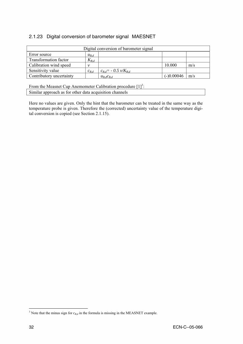
Digital conversion of barometer signal Error source uB,d Transformation factor KB,d Calibration wind speed v 10.000 m/s Sensitivity value cB,d cB,d= - 0.5 v/KB,d Contributory uncertainty uB,dcB,d (-)0.00046 m/s From the Measnet Cup Anemometer Calibration procedure [1]3: Similar approach as for other data acquisition channels Here no values are given. Only the hint that the barometer can be treated in the same way as the temperature probe is given. Therefore the (corrected) uncertainty value of the temperature digi-tal conversion is copied (see Section 2.1.15).
3 Note that the minus sign for cB,d in the formula is missing in the MEASNET example.
32 ECN-C--05-066

2.1.24 Digital conversion of barometer signal DEWI
Digital conversion of barometer signal Error source uB,d Transformation factor KB,d Calibration wind speed v 10.000 m/s Sensitivity value cB,d cB,d= - 0.5 v/KB,d Contributory uncertainty uB,dcB,d (-)0.01 m/s This standard uncertainty is estimated by DEWI of being smaller than 0.01 m/s.
ECN-C--05-066 33
2.1.25 Statistical uncertainty in the mean of the wind speed time series MEASNET
sA statistical uncertainty in the mean of the wind speed time series
Error source usA vT
samples I ⋅⋅1
0.026 m/s
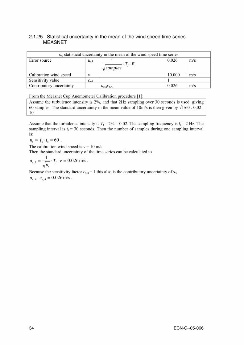
Calibration wind speed v 10.000 m/s Sensitivity value csA 1 Contributory uncertainty us,Acs,A 0.026 m/s From the Measnet Cup Anemometer Calibration procedure [1]: Assume the turbulence intensity is 2%, and that 2Hz sampling over 30 seconds is used, giving 60 samples. The standard uncertainty in the mean value of 10m/s is then given by √1/60 . 0,02 . 10 Assume that the turbulence intensity is TI = 2% = 0.02. The sampling frequency is fs = 2 Hz. The sampling interval is ts = 30 seconds. Then the number of samples during one sampling interval is:
60=⋅= sss tfn . The calibration wind speed is v = 10 m/s. Then the standard uncertainty of the time series can be calculated to
m/s026.01, =⋅⋅= vT
nu I
sAs .
Because the sensitivity factor cs,A = 1 this also is the contributory uncertainty of sA. m/s026.0,, =⋅ AsAs cu .
34 ECN-C--05-066

2.1.26 sA statistical uncertainty in the mean of the wind speed time series DEWI
sA statistical uncertainty in the mean of the wind speed time series
Error source usA vT
samples I ⋅⋅1
0.004 m/s
Calibration wind speed v 10.000 m/s Sensitivity value csA 1 Contributory uncertainty uAcA 0.004 m/s The DEWI turbulence intensity is 0.2 %. 1 Hz sampling over 30 seconds gives 30 samples. Then the standard uncertainty of the time se-ries can be calculated to
m/s004.01, =⋅⋅= vT
samplesu IAs .
Because the sensitivity factor cs,A = 1 this also is the contributory uncertainty of sA. m/s004.0, =⋅ AssA cu .
ECN-C--05-066 35

2.1.27 Humidity correction to density MEASNET
Humidity correction to density Error source uρ n/a m/s Correction factor kρ
k
wk
BPk ⋅
⋅−≈ϕ
ρ 378.01 0.997
Relative humidity ϕk 50 % Accuracy of relative humidity dϕ 5.0 % Barometric pressure Bk 101300 Pa Vapour pressure Pw Pw = 0.0000205 exp (0.0631846 T) 1655 Pa Temperature T 15 °C Calibration wind speed v 10 m/s Error source relative humidity uϕ uϕ = dϕ ϕk 0.025 m/s Sensitivity value relative hu-midity
cϕ
k
w
BP
kvc ⋅⋅⋅= 378.05.0ρ
ϕ 0.031 m/s
Contributory uncertainty in rela-tive humidity
uϕcϕ 0.00077 m/s
Assumption uρ2cρ
2 = uϕ2cϕ
2 Contributory uncertainty in hu-midity correction to density
uρcρ 0.00077 m/s
From the Measnet Cup Anemometer Calibration procedure [1]: It is possible to show that cρ
2uρ2 is equivalent to cϕ
2uϕ2 (where uρ is the uncertainty in relative
humidity and cρ is the sensitivity of derived wind speed to humidity) if cρ is dominated by cϕ rather than cB or cT. This is normally the case. Assume relative humidity, ϕ, is measured from a hand-held meter as 50% to an accuracy of 5% within 95% confidence. ϕ= 0,5 and uϕ = 0,025
BP
kvk
kvc w⋅⋅⋅=
∂∂
⋅∂∂
= 378.021
ρ
ρ
ρϕ ϕ
At 15°C, Pw = 1700 Pa and assuming B = 1013 mbar = 101300 Pa kρ is evaluated as 0,997 and cϕ (at 10m/s) is 0,032 To calculate the humidity correction to density kρ formula (7) from [1] page 13 is used:
k
wk
BPk ⋅
⋅−≈ϕ
ρ 378.01
During the calibration the value of the relative humidity was %50=kϕ . The barometric pres-sure Bk during the calibration was Bk = 101300 Pa. The temperature during the calibration was 15 °C ≡ 288.15 K. The vapour pressure for the prevailing temperature can be calculated by
Pa1655)0631846.0exp(0000205.0 ≅⋅⋅= TPw
Now kρ can be calculated to 997.0378.01 =⋅
⋅−≈k
wk
BPk ϕ
ρ .
To calculate cϕ the formula on page 21 from [1] is used:
m/s031.0378.02
=⋅⋅=∂
∂⋅
∂∂
=BP
kvk
kvc w
ρ
ρ
ρϕ ϕ
.
The accuracy of the relative humidity is given to 5% = 0.005. Therefore the standard uncertainty uϕ of the relative humidity is:
36 ECN-C--05-066

m/s025.005.0 =⋅= ku ϕϕ . The contributory uncertainty of the humidity correction to density than is
m/s00077.0=⋅ ϕϕ cu .
NOTE: In [1] erroneous numbers are used: Pa1700=wP , and
m/s032.0=ϕcm/s001.0=⋅ ϕϕ cu
2.1.28 Humidity correction to density DEWI Humidity correction to density
Error source uρ -- m/s Correction factor kρ
k
wk
BPk ⋅
⋅−≈ϕ
ρ 378.01 0.997
Relative humidity ϕk 31.7 % Accuracy of rel. humidity dϕ 5.0 % Barometric pressure Bk 101690 Pa Vapour pressure Pw Pw = 0.0000205 exp (0.0631846 T) 2527 Pa Temperature T 294.85 K Calibration wind speed v 10.000 m/s Error source rel. humidity uϕ uϕ = dϕ ϕk 0.016 m/s Sensitivity value relative hu-midity
cϕ
k
w
BP
kvc ⋅⋅⋅= 378.05.0ρ
ϕ 0.0471 m/s
Contributory uncertainty in relative humidity
uϕcϕ 0.00075 m/s
Assumption uρ2cρ
2 = uϕ2cϕ
2 Contributory uncertainty in humidity correction to density
uρcρ 0.00075 m/s
To calculate the humidity correction to density kρ formula (7) from [1] page 13 is used:
k
wk
BPk ⋅
⋅−≈ϕ
ρ 378.01
During the calibration the value of the relative humidity was %7.31=kϕ . [3] The barometric pressure Bk during the calibration was Bk = 101690 Pa. [3] The temperature during the calibration was T = 21.7 °C ≡ 294.85 K. [3] The vapour pressure for the prevailing temperature can be calculated by
Pa2527)0631846.0exp(0000205.0 =⋅⋅= TPw
Now kρ can be calculated to 997.0378.01 =⋅
⋅−≈k
wk
BPk ϕ
ρ .
To calculate cϕ the formula on page 21 from [1] is used:
m/s0471.0378.02
=⋅⋅=∂
∂⋅
∂∂
=BP
kvk
kvc w
ρ
ρ
ρϕ ϕ
.
The accuracy of the relative humidity is given to 5% = 0.005. Therefore the standard uncertainty uϕ of the relative humidity is:
m/s01585.005.0 =⋅= ku ϕϕ . The contributory uncertainty of the humidity correction to density is:
m/s00075.0=⋅ ϕϕ cu .
ECN-C--05-066 37

2.2 Total type B uncertainty MEASNET
Contributory type B uncertainty ui Value [m/s] 1. Wind tunnel correction 2. Wind tunnel calibration 3. Pressure transducer sensitivity 4. Pressure transducer signal conditioning gain 5. Pressure transducer data sampling conversion 6. Ambient temperature transducer 7. Temperature signal conditioning gain 8. Temperature signal digital conversion 9. Pitot tube head coefficient 10. Sensitivity of barometer 11. Signal conditioning gain on barometer 12. Digital conversion of barometer signal 13. sA statistical uncertainty in the mean of the wind speed time series 14. Humidity correction to density
0.025 0.049 0.034 0.01
0.0029 0.0014
0.002 0.00046
-0.005 0.0014
0.002 0.00046
0.026 0.00077
Total type B uncertainty ∑=i
iB uu 2 0.07
38 ECN-C--05-066

2.3 Total type B uncertainty DEWI
Contributory type B uncertainty ui Value [m/s] 1. Wind tunnel correction 2. Wind tunnel calibration 3. Pressure transducer sensitivity 4. Pressure transducer signal conditioning gain 5. Pressure transducer data sampling conversion 6. Ambient temperature transducer 7. Temperature signal conditioning gain 8. Temperature signal digital conversion 9. Pitot tube head coefficient 10. Sensitivity of barometer 11. Signal conditioning gain on barometer 12. Digital conversion of barometer signal 13. sA statistical uncertainty in the mean of the wind speed time series 14. Humidity correction to density
0.0001 0.005 0.017
0 0.01
0.0034 0.001 0.01
-0.005 -0.01 0.01 0.01
0.004 0.00075
Total type B uncertainty ∑=i
iB uu 2 0.03
ECN-C--05-066 39

2.4 Comparisons
In the table below the differences between Version 1 of the Measnet cup calibration procedure [1] and the power performance procedure under proposal [2] are summarised, together with dif-ferences found to the analysis presented in this report in Section 2.1. Error source, item Previous [1]
procedure Proposed [2] procedure
Derived
up,t , standard uncertainty calibr. point up,t , contributory uncertainty up,d , standard uncertainty quantisation limit up,d , no. of bits for voltage at cal. point up,d , conversion uncertainty up,d , sensitivity value cp,d up,d , contributory uncertainty uT,d , st. uncertainty quantisation limit uT,d , conversion uncertainty uT,d , sensitivity value cT,d uT,d , contributory uncertainty uB,s , sensitivity value cB,s= uB,d , sensitivity value cB,d= uρ , vapour pressure uρ , sensitivity value relative humidity uρ , contributory uncertainty
33 0.033
0.00704
490 0.000002 2049 0.004
0.00704 0.0000023 2049 0.004
0.5 v/KB,s 0.5 v/KB,d
1700 0.032 0.001
33 0.033
0.000704
490 0.000002 2049 0.004
0.000704 0.0000023 2049 0.004
0.5 v/KB,s 0.5 v/KB,d
1700 0.032 0.001
34 0.034
0.000705
492 0.0000014 2048 0.0029
0.000705 0.00000023 2048 0.00046
- 0.5 v/KB,s - 0.5 v/KB,d
1655 0.031 0.00077
This list summarises the (minor) mistakes in the MEASNET document for cup-anemometer calibrations [1] and the proposal for the IEC document on power performance measurements [2]. This list has been handed over to the IEC with the recommendation to correct these.
40 ECN-C--05-066

3. Cup anemometer calibration uncertainty: TYPE A
3.1 Introduction
The type A uncertainty is defined by ISO [4] as a method of evaluation of uncertainty by the statistical analysis of series of observations. Basically it is an uncertainty analysis based on sta-tistics. The MEASNET document [1] gives the formulas how to calculate these type A uncertainties on pages 34 to 36. This calculation was analysed in detail to understand the background. In this re-port it is assumed that all necessary requirements regarding the statistical model for linear cali-bration are valid and that therefore the general theory for linear calibration [8] can be used.
3.2 Standard MEASNET calibration
In the standard calibration for cup anemometers according to MEASNET the main steps of the calibration are: • 5 minute run in for the cup anemometer • Take calibration points at rising and falling wind speeds between 4 to 16 m/s (a suggested
sequence is 4, 6, 8, 10, 12, 14, 16, 15, 13, 11, 9, 7, 5 m/s) • Sampling frequency shall be at least 1 Hz and the sampling interval shall be at least 30 sec-
onds • Data collection can only start after stable flow conditions have established (this takes nor-
mally 1 minute at each wind speed) In the data analysis an inverse regression is done by regressing the wind speed on the anemome-ter output. The data is averaged to a 30 second average and then the regression analysis is done, together with the type A uncertainty analysis for the regression. However, an important point is that the regression is done over 30 second intervals, whereas for power performance measurements data are averaged over 10-minute intervals. Since a main characteristic of type A uncertainty is that it can be reduced by extra measurements (it is based on statistics of the data set), this raises the question if the calculated uncertainty for the regres-sion is the best estimate for the type A uncertainty for calibration, when data is taken with 10-minute intervals. When doing the regression analysis we can distinguish between the number of data points at each wind speed (N) and the time each data point represents (M). The standard calibration would have N=1 and M=30 seconds. In this Chapter we will investigate whether the calibration uncertainty depends on N or M.
3.3 DNW wind tunnel measurements
To answer this question data taken in a wind tunnel have been analysed. For the measurements the DNW-LST wind tunnel has been used, which is a very accurate, low turbulence wind tunnel in the Netherlands. Instead of taking an average over 30 seconds at each wind speed (with a sample frequency of at least 1 Hz) 1 second measurements are done at each wind speed, with 100 samples at each wind speed. This way various calibrations with various combinations of the values for N and M can be performed. An overview of the calibrations that have been performed is presented in Table 3-1.
ECN-C--05-066 41

Table 3-1. Overview of the various combinations of the values for N and M
Calibration cycle 1 4(2)16, 15(-2)5 13 wind speedsUncertainty interval α = 0.05
Run no. NNo. of points n in regression
n-2 used for tα/2 tα/2,n-2
0 1 * 1sec per WS 1 1 sec 13 11 2.2011 2 * 1sec per WS 2 1 sec 26 24 2.0642 5 * 1sec per WS 5 1 sec 65 60 2.0003 10 * 1sec per WS 10 1 sec 130 120 1.9804 20 * 1sec per WS 20 1 sec 260 infinite 1.9605 50 * 1sec per WS 50 1 sec 650 infinite 1.9606 100 * 1sec per WS 100 1 sec 1300 infinite 1.960
Calibration cycle 2 4(2)16, 15(-2)5 13 wind speedsUncertainty interval α = 0.05
Run no. NNo. of points n in regression
n-2 used for tα/2 tα/2,n-2
0 1 * 1 sec per WS 1 1 sec 13 11 2.2011 1 * 2 sec per WS 1 2 sec 13 11 2.2012 1 * 5 sec per WS 1 5 sec 13 11 2.2013 1 * 10 sec per WS 1 10 sec 13 11 2.2014 1 * 20 sec per WS 1 20 sec 13 11 2.2015 1 * 50 sec per WS 1 50 sec 13 11 2.2016 1 * 100 sec per WS 1 100 sec 13 11 2.201
Calibration cycle 3 4(2)16, 15(-2)5 13 wind speedsUncertainty interval α = 0.05
Run no. NNo. of points n in regression
n-2 used for tα/2 tα/2,n-2
0 1 * 10 sec per WS 1 10 sec 13 11 2.2011 2 * 10 sec per WS 2 10 sec 26 24 2.0642 5 * 10 sec per WS 5 10 sec 65 60 2.0003 10 * 10 sec per WS 10 10 sec 130 120 1.980
Calibration cycle 4 4(2)16, 15(-2)5 13 wind speedsUncertainty interval α = 0.05
Run no. NNo. of points n in regression
n-2 used for tα/2 tα/2,n-2
0 2 * 1 sec per WS 2 1 sec 26 24 2.0641 2 * 2 sec per WS 2 2 sec 26 24 2.0642 2 * 5 sec per WS 2 5 sec 26 24 2.0643 2 * 10 sec per WS 2 10 sec 26 24 2.0644 2 * 20 sec per WS 2 20 sec 26 24 2.0645 2 * 50 sec per WS 2 50 sec 26 24 2.064
Calibration cycle 5 4(2)16, 15(-2)5 13 wind speedsUncertainty interval α = 0.05
NNo. of points n in regression
n-2 used for tα/2 tα/2,n-2
IEA 2 * 30 sec per WS 2 30 sec 26 24 2.064MEASNET 1 * 30 sec per WS 1 30 sec 13 24 2.064
N.B. the notation 4(2)16, 15(-2)5 designates the wind tunnel speed cycle, from 4 to 16 withsteps of 2 m/s and then from 15 to 5 with steps of -2 m/s. The resulting cycle is 4, 6, 8, 10,12, 14, 16, 15, 13, 11, 9, 7, 5 m/s.
M
M
M
M
M
42 ECN-C--05-066

The uncertainty that is reported is calculated according to Montgomery [8] and it is the standard deviation of the Y-estimate. From Table 3-1 can be seen that calibrations series have been done where the number of data points per wind speed have been kept constant while the time per data point varied, as well as vice-versa.
3.4 Linear regression analysis
The data from the calibration measurements will be analysed using a simple linear regression model [8]:
εββ ++= xy 10 (1) with the intercept β0 and the slope β1 as unknown constants called regression coefficients and a random error component ε. The error components are assumed to have mean zero, E(ε)=0, and unknown variance σ2. Furthermore it is assumed that the errors are uncorrelated. Formula (1) is called the population regression model.
3.4.1 Estimate of the regression coefficients When n pairs of data (yi, xi) are available, formula (1) can be rewritten to a sample regression model:
iii xy εββ ++= 10 (2) The method of least squares is used to estimate β0 and β1 i.e. the sum of the squares of the dif-ferences between the observations yi and the straight regression line is a minimum. The estima-tors of β0 and β1 are denoted as and . The solution of the least squares minimisation of (2) is:
0β 1
β
xy 10
ββ += (3) with
∑=
=n
iiy
ny
1
1 ∑
=
=n
iix
nx
1
1 (4)
and
∑∑
∑∑∑
=
=
===
⎟⎠
⎞⎜⎝
⎛
−
⎟⎠
⎞⎜⎝
⎛⎟⎠
⎞⎜⎝
⎛−
=
n
i
n
ii
i
n
ii
n
ii
n
iii
n
xx
xyn
xy
1
2
12
1111
1
β (5)
The estimator of the slope can be rewritten to 1
β
xx
xyn
ii
n
iii
SS
xx
xxy=
−
−=
∑
∑
=
=
1
2
11
)(
)(β (6)
The residual is defined as the difference between the observed value yi and and the corre-
sponding fitted value , ie
iy ( )iiiiie = xyyy 10 ββ +−=− .
ECN-C--05-066 43

3.4.2 Estimation of uncertainties First an estimation of σ2 is determined following [8]. The estimate of σ2 is obtained using the residual, or error sum of squares:
∑ ∑=
−==n
iiiis yyeSS
1
22Re )( (7)
where yi are the observed values and the fitted values. Using equation (7) can be rewritten to
iy ii xy 10 ββ +=
xy
n
iis SynySS 1
2
1
2Re
β−−=∑=
or to
xyTs SSSSS 1Reβ−=
with
∑∑==
−=−=n
ii
n
iiT yyynySS
1
22
1
2 )(
The expected value of SSRes is
2Re )2()( σ−= nSSE s (8)
since the residual sum of squares has (n-2) degrees of freedom, because two degrees of freedom are associated with the estimates and . Hence an unbiased estimator of is 0
β 1β 2σ
ss MS
nSS
ReRe2
)2( =
−=σ (9)
The quantity MSRes is called the residual mean square. The quantity 2σ is also called the standard error of regression. Any violation of the model assumptions or misspecification of the model form may however affect the usefulness of as an estimate of , therefore it is a model-dependent estimate of .
2σ 2σ2σ
Next an estimation of the uncertainty in the regression parameters is determined. The variance in the parameters and is given by [8]: 1
β 0β
xxSVar
2
1)( σβ = (10)
and, since the covariance between y and is zero, 1β
⎟⎟⎠
⎞⎜⎜⎝
⎛+=+=
xxSx
nVarxyVarVar
22
12
01)()()( σββ (11)
with
nyVar
2
)( σ= (12)
44 ECN-C--05-066

The covariance between the regression parameters and is given by: 0β 1
β
xxSxCov
2
10 ),( σββ −= (13)
The variance of a single data point yi given the n measurements (xi, yi) is given by [8]:
),(2)()()( 10012 ββββ CovxVarVarxyVar iii ++= (14)
3.4.3 Uncertainty in the prediction of new observations With the analysis shown in section 3.4.1 it is possible to predict new observations using the re-gression coefficients. Therefore the following regression equation can be used:
0100 xy ββ += (15)
with x0 the value of the regressor variable of interest and the point estimate of the new value of response y0. For the prediction of the value of new observations, a prediction interval must be determined from the distribution.
0y
A (1-α) prediction interval on a future observation y0 is now [8]:
⎟⎟⎠
⎞⎜⎜⎝
⎛ −++±= −
xxsn S
xxn
MStyy2
0Re2,2/00
)(11 α (16)
with tα/2, n-2 the percentage point of the t-Distribution with n-2 degrees of freedom. The predic-tion interval (16) widens as xx −0 increases.
3.5 Methodology
3.5.1 Averaging To perform the regression analysis with the calibration data as shown in Table 3-1 in case M > 1 seconds the following additions to section 3.4 can be made:
∑=
=M
jjki s
My
1,
1 ∑
=
=M
jjki f
Mx
1,
1 (17)
with sk,j the wind tunnel speed and fk,j the cup anemometer frequency at sample j (seconds) and wind speed k (m/s). The range of k is listed in Table 3-1 and is from 4 to 16 m/s in steps of 2 m/s and from 15 to 5 m/s in steps of -2 m/s, these are 13 wind speeds in total. The range of i therefore is [13N], this equals [n]. The range of M is also listed in Table 3-1 and is [1, 2, 5, 10, 20, 30, 50, 100] seconds. Note that N is the number of data points at each wind speed in the lin-ear regression analysis and M the time each data point represents (see section 3.2).
3.5.2 Prediction table and uncertainty calculation After the regression analysis and the determination of the regression coefficients (equations 3 & 6) a prediction table is made using these coefficients and the uncertainty calculation in the pre-diction of new observations (equation 10). The prediction for new observations is done using
ECN-C--05-066 45

frequencies belonging to 13 wind speeds of = 4 to 16 m/s in steps of 1 m/s. The resulting un-certainties are averaged per run in a cycle (see Table 3-1):
0y
⎟⎟⎠
⎞⎜⎜⎝
⎛ −−++== ∑∑
=−
= xxs
yna
yyrcrc S
xyn
MStuU 21
2100
Re
16
42,2/
16
4,,,
)(11131
131
00
0 βββ
(18)
with Uc,r the averaged uncertainty for cycle c and run r.
3.5.3 Examples of uncertainty calculation Two examples will be given here of the uncertainty analysis using inverse regression for the Risø cup, for N=2 and M=1 and for N=1 and M=2. Example with N=2 and M=1 This example is equivalent to cycle 1 run 1, with 2 regression data points per wind speed over 1 second per regression point. Note that cycle 1 run 0 and cycle 2 run 0 are actually equivalent. Table 3-2. Regression data cycle 1 run 1
s [m/s] f [Hz] yi xi 4.01366 6.11 4.01366 6.11
4.02924 6.11 4.02924 6.11
5.00103 7.72 5.00103 7.72
5.00125 7.72 5.00125 7.72
6.04819 9.42 6.04819 9.42
6.04819 9.34 6.04819 9.34
7.02091 11.07 7.02091 11.07
7.02091 11.07 7.02091 11.07
8.05948 12.68 8.05948 12.68
8.06205 12.68 8.06205 12.68
8.99809 14.11 8.99809 14.11
9.00096 14.11 9.00096 14.11
10.07100 15.91 10.07100 15.91
10.07330 15.85 10.07330 15.85
11.00340 17.41 11.00340 17.41
11.00340 17.41 11.00340 17.41
12.03890 19.11 12.03890 19.11
12.03890 19.08 12.03890 19.08
12.98760 20.72 12.98760 20.72
12.98810 20.47 12.98810 20.47
14.01550 22.32 14.01550 22.32
14.01410 22.12 14.01410 22.12
15.01870 23.84 15.01870 23.84
15.02280 23.70 15.02280 23.70
15.94700 25.25 15.94700 25.25
15.94830 25.25 15.94830 25.25
Table 3-3. Prediction table cycle 1 run 1
0x [Hz] 0y [m/s]0,1,1 yu [m/s]
6.13 4 0.0991
7.74 5 0.0978
9.34 6 0.0967
10.95 7 0.0958
12.55 8 0.0951
14.16 9 0.0948
15.76 10 0.0946
17.37 11 0.0948
18.97 12 0.0951
20.58 13 0.0958
22.18 14 0.0966
23.79 15 0.0977
25.39 16 0.0990 The average uncertainty is: U1,1 = 0.0964 m/s
In this case tα/2,n-2 = 2.064 (see Table 3-1) with a confidence interval of (1-α) = 95%. The regres-sion coefficients are: slope = 0.62288 m and intercept = 0.18200 m/s. The prediction ta-ble is shown in Table 3-3.
1β 0
β
46 ECN-C--05-066

Example with N=1 and M=2 This example is equivalent to Cycle 2 run 1, with 1 regression data point per wind speed over 2 seconds averaged per regression point. In this case tα/2,n-2 = 2.201 (see Table 3-1) with a confi-dence interval of (1-α) = 95%. The regression coefficients are: slope = 0.62293 m and inter-
cept = 0.18129 m/s. The prediction table is presented in Table 3-5. 1
β
0β
Table 3-4. Regression data cycle 2 run 1
s [m/s] f [Hz] yi xi
4.01366 6.11 4.02145 6.11
4.02924 6.11
5.00103 7.72 5.00114 7.72
5.00125 7.72
6.04819 9.42 6.04819 9.38
6.04819 9.34
7.02091 11.07 7.02091 11.07
7.02091 11.07
8.05948 12.68 8.06077 12.68
8.06205 12.68
8.99809 14.11 8.99953 14.11
9.00096 14.11
10.07100 15.91 10.07215 15.88
10.07330 15.85
11.00340 17.41 11.00340 17.41
11.00340 17.41
12.03890 19.11 12.03890 19.10
12.03890 19.08
12.98760 20.72 12.98785 20.60
12.98810 20.47
14.01550 22.32 14.01480 22.22
14.01410 22.12
15.01870 23.84 15.02075 23.77
15.02280 23.70
15.94700 25.25 15.94765 25.25
15.94830 25.25
Table 3-5. Prediction table cycle 2 run 1
0x [Hz] 0y [m/s]0,1,1 yu [m/s]
6.13 4 0.0792
7.74 5 0.0773
9.34 6 0.0757
10.95 7 0.0744
12.55 8 0.0735
14.16 9 0.0729
15.76 10 0.0727
17.37 11 0.0729
18.97 12 0.0734
20.58 13 0.0744
22.18 14 0.0756
23.79 15 0.0772
25.39 16 0.0791 The average uncertainty is U2,1 = 0.0753 m/s
ECN-C--05-066 47

3.6 Uncertainty of the regression
In this Section, the uncertainty of the regression applied to the cup anemometer calibration data is investigated for the same cup anemometer calibrated in the DEWI wind tunnel and the DNW wind tunnel. The uncertainties of the regression for the Risø cup anemometer in the DEWI wind tunnel are presented in Table 3-6, those of the DNW wind tunnel are presented in Table 3-7. Sya is the standard deviation for y according to the MEASNET document (eq. 14), Ua is the re-sulting type A standard uncertainty, with a confidence interval of 95% (k = 2). The resulting un-certainty of the applied regression is quite similar for the DNW and the DEWI wind tunnel. The type A uncertainties according [1] are larger than these uncertainties attached to the regression (See also Appendix A).
Table 3-6. Calibration data and uncertainties of a Risø cup in the DEWI wind tunnel
Tunnel speed Cup freq Sya Ua [m/s] [Hz] [m/s] [m/s] 4.301 6.515 0.0091 0.0181 5.351 8.188 0.0079 0.0159 6.343 9.750 0.0070 0.0139 7.448 11.500 0.0060 0.0120 8.372 13.063 0.0053 0.0106 9.425 14.719 0.0049 0.0097
10.219 16.032 0.0047 0.0095 11.230 17.656 0.0049 0.0098 12.322 19.355 0.0054 0.0108 13.298 20.909 0.0061 0.0122 14.382 22.688 0.0071 0.0142 15.167 23.938 0.0079 0.0158 15.762 24.903 0.0085 0.0171
Table 3-7. Calibration data and uncertainties of a Risø cup in the DNW wind tunnel
Tunnel speed Cup freq Sya Ua [m/s] [Hz] [m/s] [m/s]
4.0152627 6.1807 0.00911 0.01823 4.9973663 7.7497 0.00807 0.01613 6.0331980 9.4390 0.00702 0.01404 7.0183713 10.9727 0.00618 0.01236 8.0561847 12.6767 0.00542 0.01085 9.0007093 14.1047 0.00500 0.01000
10.0748600 15.8923 0.00481 0.00963 11.0041933 17.3157 0.00497 0.00994 12.0367333 18.9813 0.00546 0.01093 12.9926767 20.5317 0.00615 0.01231 14.0130000 22.1910 0.00707 0.01413 15.0214667 23.7813 0.00805 0.01611 15.9471967 25.2830 0.00905 0.01811
48 ECN-C--05-066

3.7 Results of the analysis
These calibrations have been done for six different cup anemometers: three different Mierij cup anemometers, a Risø cup anemometer, a Lambrecht cup anemometer and an NRG cup anemometer. The results from the Risø cup anemometer and the Mierij cup anemometer (ECN identification DEST0005) for cycle 1 and 4 can be seen in Figure 3-1 and Figure 3-2. In these figures no clear dependency can be observed of the number of points per wind speed and the calibration uncertainty.
Calibration uncertainty RisoNumber of points per wind speed varies
Time per data point = 1 sec
0
0.02
0.04
0.06
0.08
0.1
0.12
0.14
0 20 40 60 80 100
Number of points per wind speed
Unc
erta
inty
(m/s
)
120
Figure 3-1 Calibration uncertainty versus the number of data points per wind speed for the Risø
cup anemometer, cycle 1
Calibration uncertainty DEST0005Number of points per wind speed varies
Time per data point = 1 sec
0
0.05
0.1
0.15
0.2
0.25
0 20 40 60 80 100
Number of points per wind speed
Unc
erta
inty
(m/s
)
120
Figure 3-2 Calibration uncertainty versus the number of data points per wind speed for the
Mierij cup anemometer DEST0005, cycle 1
ECN-C--05-066 49

Calibration uncertainty Riso,Number of data points per wind speed = 2
Time per data point varies
0
0.02
0.04
0.06
0.08
0.1
0.12
0 10 20 30 40 50 6
Averaging time
Unc
erta
inty
(m/s
)
0
Figure 3-3 Calibration uncertainty versus the time per data point for the Risø cup anemometer,
cycle 4
Calibration uncertainty DEST0005Number of points per wind speed = 2
Time per data point varies
0
0.02
0.04
0.06
0.08
0.1
0.12
0.14
0.16
0.18
0 10 20 30 40 50 6
Averaging time
Unc
erta
inty
(m/s
)
0
Figure 3-4 Calibration uncertainty versus the time per data point for the Mierij cup anemometer
DEST0005, cycle 4 From Figure 3-3 and Figure 3-4, a dependency is observed of the time per data point on the calibration uncertainty. From these results the conclusion is drawn that the number of data points per wind speed does not have a noticeable influence on the calibration uncertainty of these two cups. For the time per data point the picture is completely different. It is observed that the uncertainty decreases with increasing averaging time.
50 ECN-C--05-066

Calibration uncertainty RisoNumber of points per wind speed = 2
Time per data point varies
y = 0.1064x-0.3015
R2 = 0.9239
0
0.02
0.04
0.06
0.08
0.1
0.12
0 10 20 30 40 50 60
Averaging time
Unc
erta
inty
(m/s
)
Wind tunnel dataSquare root lawPower function
Figure 3-5 Fitting the relationship between the uncertainty and M using the square root law and
a power function For the Risø cup anemometer a relationship has been tried to find between M and the uncer-tainty, see Figure 3-5. A fit of the data with a power function leads to an empirical relationship between the uncertainty (y) and the time per data point (M):
(19) 3015.0*1064.0 −= My This is an empirical relationship that is not intuitive. The Guide to the expression of uncertainty in measurement [4] (GUM) gives the following relationship:
nqs
qs k )()(
22 = (20)
This gives the relationship between the best estimate of the variance (s) of a quantity q that has been measured n times. In line with the previous equation a good fit is found when using:
41,
,
^
^
MMy
My
=∝σ
σ (21)
This gives the relationship between the standard deviation of the Yestimate and the time per data point (M). This function (21) fits as well as the power function and intuitively agrees to the GUM.
ECN-C--05-066 51

3.8 Response of cup anemometer in wind tunnel
The requirements of cup anemometer calibrations state a minimum sample frequency of 1Hz. Experiments using cup anemometers in wind tunnels have shown unstable behaviour of the cup anemometers themselves. In this section, we summarise some of the results of measurements in wind tunnels as performed by Frank Ormel in 2003. The measurements have been done in the German-Dutch DNW wind tunnel. The applied cup anemometers are summarised in Table 3-8. The cup anemometers are compared to measurements using a propeller anemometer. It is shown in Figure 3-6 and Figure 3-7 that the propeller anemometer has a very stable response, although it is able to measure fast fluctuations in wind speed. This shows that the wind speed of the tun-nel is very stable. The fluctuating cup anemometer response is therefore the result of the cup anemometers themselves. This typical behaviour has been confirmed by measurements of FOI [9] in the FOI LT5 wind tunnel and the KTH-MTL tunnel that has turbulence levels lower than 0.025%. Table 3-8. Overview of cup anemometers used in the analysis. Brand Type ECN identification number Reference Mierij 018 DEST0005 Mierij 1 Mierij 019 DEWS0299 Mierij 2 Mierij 020 DEWS0418 Mierij 3 Lambrecht DEWS0230 Lambrecht NRG Max40 dynamo DEWS0366 NRG Riso P2546 DEWS0600 Riso Gill R3A sonic DEWS0583 Gill
The measurements using the propeller anemometer have been confirmed in a separate meas-urement campaign. In these measurements, the propeller anemometer is compared to measure-ments with a Gill sonic anemometer. The responses of these anemometers are quite similar and show the same standard deviation around the mean. Compared to cup anemometers, the propel-ler and Gill sonic anemometer measure the relatively stable wind speed of the tunnel more accu-rate and it has been confirmed that the fluctuating response of cup anemometers is due to the cup anemometer itself. The findings of these experiments support the findings in the previous section. The averaging time of wind speed measurements by cup anemometers in wind tunnels should be increased to reduce the cup anemometer calibration uncertainty. When the averaging time is increased, the fast fluctuations are averaged out and the standard deviation of the points in the regression of the cup anemometer calibration are reduced.
52 ECN-C--05-066

Figure 3-6. Shown is the comparison of wind speed measurements with a cup anemometer and a
propeller anemometer. A Mierij (DEST0005), a Risø and a Lambrecht cup anemometer are compared to the propeller.
Figure 3-7. Shown is the comparison of wind speed measurements with a cup anemometer and a
propeller anemometer. An NRG, and two Mierij (DEWS0299 and DEWS0418) cup anemometers are compared to the propeller.
ECN-C--05-066 53

3.9 Discussion
The variability of cup anemometers in wind tunnels leads to fluctuations in the wind speed measurements that originate from the unstable wakes behind the cups. Since the requirements on cup anemometer calibration require sample frequencies larger than 1Hz, these fluctuations are captured in the calibration procedure. Given the remarkable linearity of cup anemometers against wind speed, the regression through the averaged measurements of the calibration proce-dure leads to much smaller uncertainties. One could argue whether a minimum sample fre-quency of 1 sec would lead to higher type A uncertainties than longer averaging periods. The averaged values of the measurements using cup anemometers are much better than one would suspect from the variation in wind speed measurements during the 30-second period. This report will be followed by a request for information at MEASNET accredited wind tunnels, focussing on typical values for the type A and type B uncertainties of Risø cup anemometers and spread in measurements using the so-called golden reference cup anemometers. For the ten Risø cup anemometers that are calibrated at the same day at DEWI, the type A un-certainty at 10m/s is determined using the derived type B uncertainty (see Chapter 2). In Figure 3-8 the total uncertainties (1σ) and the derived type A uncertainties are shown using the type B uncertainty of 0.03 m/s, as derived in Chapter 2. In the case of the DEWI wind tunnel, the type A uncertainty is of the order of the type B uncertainty or larger and has a large spread.
Uncertainties cup anemometer calibration @10m/s
0.00
0.01
0.02
0.03
0.04
0.05
0.06
0.07
0.08
Riso cup279_03
Riso cup278_03
Riso cup277_03
Riso cup276_03
Riso cup275_03
Riso cup274_03
Riso cup273_03
Riso cup272_03
Riso cup271_03
Riso cup270_03
Unc
erta
inty
[m/s
]
Total uncertainty @10m/s
Derived type A uncertainty @10m/s
Figure 3-8. The total uncertainties and the derived type A uncertainties are shown for the ten
Risø cup anemometers that are calibrated at the same day at DEWI. The type B uncertainty derived in Chapter 2 has been used (=0.03m/s).
54 ECN-C--05-066

4. Conclusions
ECN calibrates its cup-anemometers in the DEWI wind tunnel. For power performance meas-urements under MEASNET and IEC regulations uncertainty analyses are important. Since the calibration uncertainty is a large contribution to the uncertainty analysis in power performance measurements, ECN started the analyses of the reported uncertainties in the DEWI wind tunnel. Since DEWI does not report the type A and type B uncertainties separately, this poses a prob-lem for the analysis. Both types of uncertainties are investigated separately. A detailed analysis of the type B uncertainty has been performed. The analyses showed (minor) mistakes in the MEASNET document for cup-anemometer calibrations [1] and the proposal for the IEC document on power performance measurements [2]. This led to recommendations to the IEC, see section 2.4. The type A uncertainty of the cup anemometer calibration can be derived from the combined calibration uncertainty of the DEWI calibrations now the value for the type B uncertainty has been determined. ECN has calibrated ten anemometers at a single day and the spread in type A uncertainty is rather large, ranging from 0.026m/s to 0.063m/s. The analysis of type A uncertainties starts with a description of the uncertainty of the regression. It has been shown that the measurements of cup anemometers include variations that originate from the cup itself. The resulting type A uncertainty, determined by these fluctuations, is larger than would be necessary based on the regression analysis. Although the cup anemometer fluctu-ates on small time scales, the averaged values show very good linearity against wind speed. It should be investigated whether other averaging schemes during cup anemometer calibrations could reduce the associated uncertainties.
ECN-C--05-066 55

5. References
[1] Measnet Cup Anemometer Calibration Uncertainty, Version 1 September 1997 [2] IEC 61400-121, Wind turbine generator systems- Part 12: Wind Turbine Power Per-
formance testing [3] Calibration Certificate 279-03, DEWI Wilhelmshaven, 27 March 2003 [4] Guide to the expression of uncertainty in measurement, corrected and reprinted 1995,
International Organisation for Standardization, Geneva 91995). [5] D. C. Montgomery, E. A. Peck, G. G. Vining, Introduction to linear regression analy-
sis, third edition, John Wiley & sons, inc New York (2001). [6] MEASNET Power performance measurement procedure, version 3, November 2000,
Network of European Measuring Institutes, (2000). [7] J. P. Molly et al, Implementation of the Network of European Measuring Institutes,
MEASNET, subproject VI of project European Wind turbine Standards II, DEWI, Wil-helmshaven (1998).
[8] Jan-Åke Dahlberg, 'Some aspects of cup anemometer behaviour and its effect on cali-
bration', presentation at IMTS 2003, FOI/FFA
56 ECN-C--05-066

Appendix A Calibration Report 279_3 from 27.03.2003
ECN-C--05-066 57

58 ECN-C--05-066
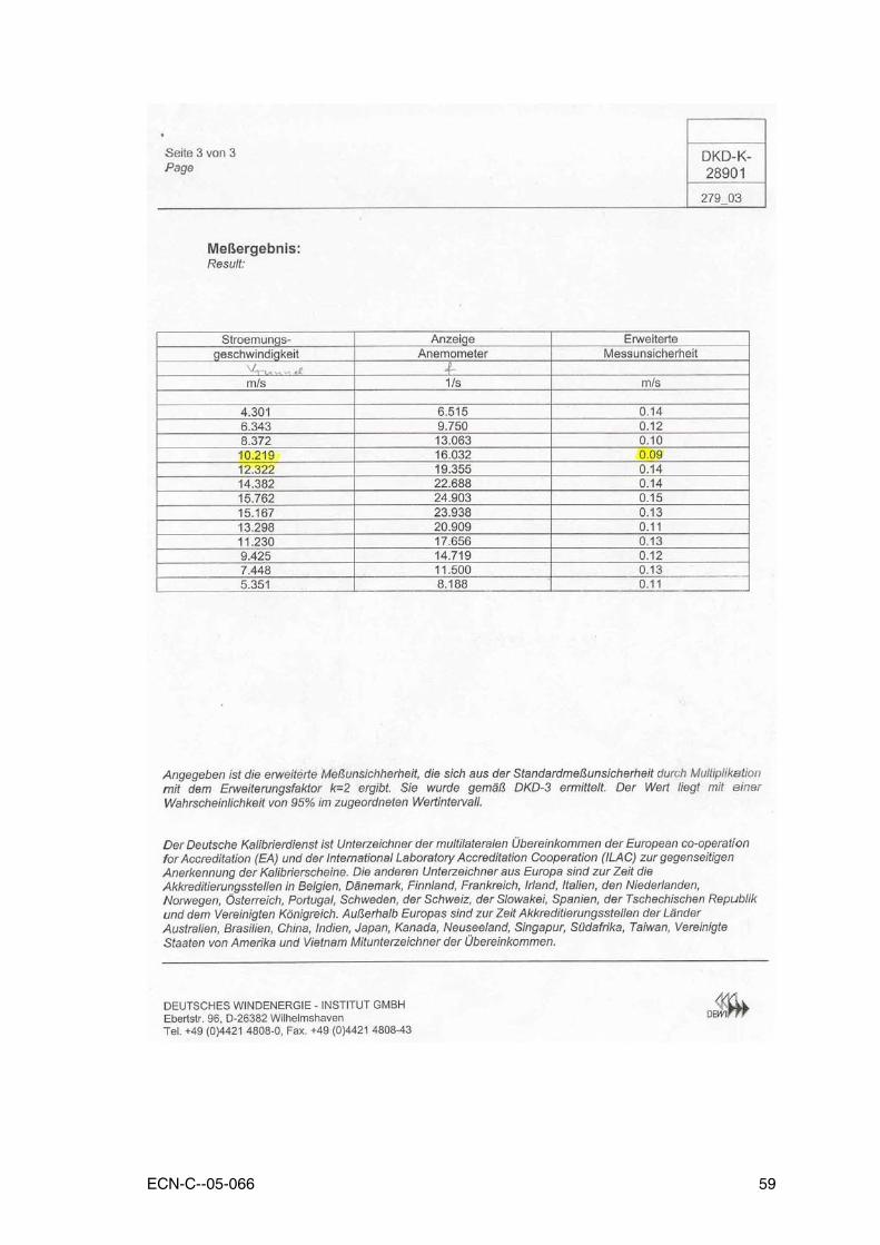
ECN-C--05-066 59

60 ECN-C--05-066

ECN-C--05-066 61

62 ECN-C--05-066