


Languages
Pages
Legal


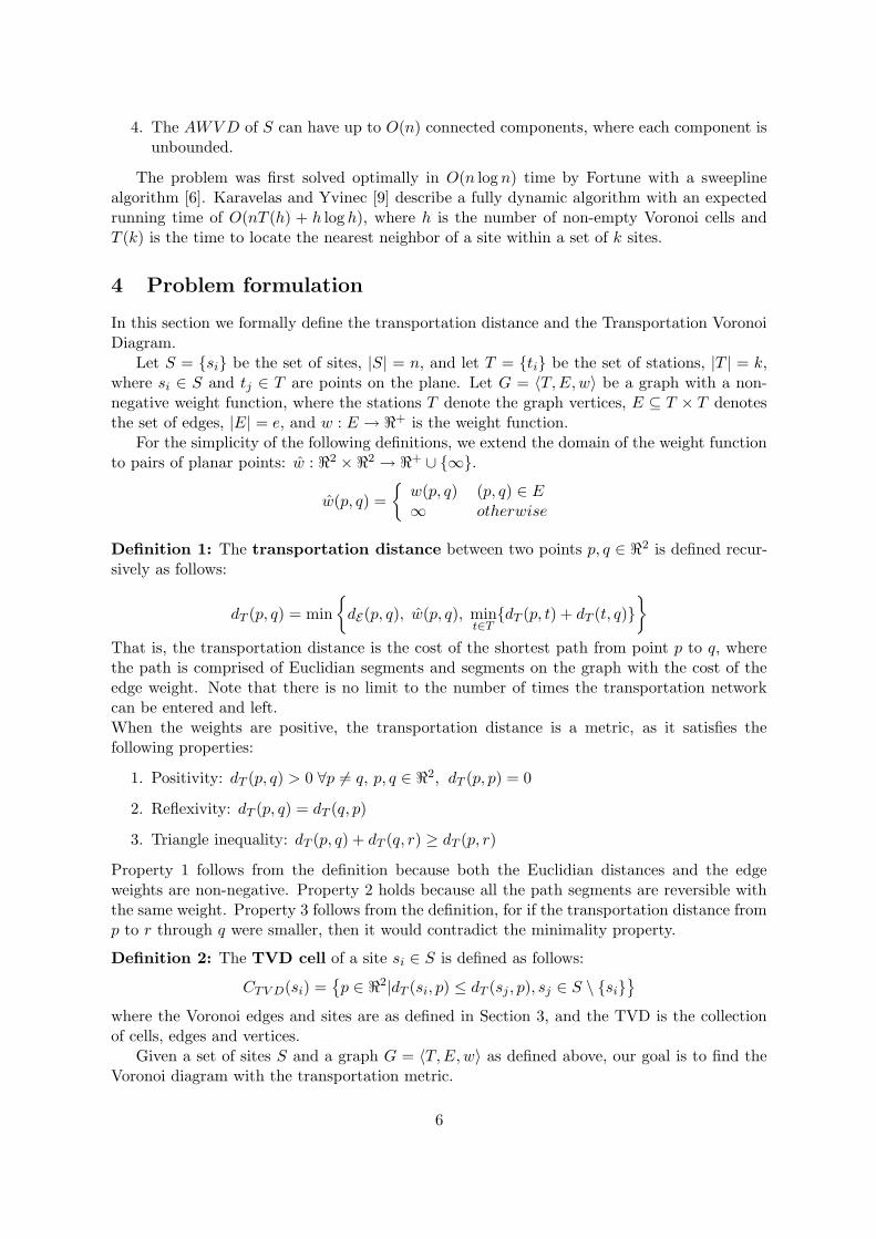
Transportation Voronoi Diagrams
Yaron Ostrovksy-Berman
School of Computer Science and Engineering
The Hebrew University of Jerusalem, Jerusalem 91904, Israel
Email: [email protected]
March 23, 2003
Abstract
The standard Voronoi diagram partitions the plane into cells with a common closestsite in Euclidian distance. We extend this model by adding a transportation network thatprovides fixed, time-saving routes. In the transportation metric, the distance betweentwo points is measured by the shortest path consisting of Euclidian segments travelledin a straight line by foot, and segments travelled on transportation lines. We model thetransportation network as an undirected graph with non-negative weights and describethe Voronoi diagram in the transportation metric. We show how to reduce it to theAdditively Weighted Voronoi Diagram (AWVD) problem. Given n sites, k stations with etransportation lines, we describe an input sensitive reduction algorithm with a worst-casecomplexity of O(k2 + (n + k) log n), or O(k log k + (n + k) log n + e) for more realistictransportation models. We present two heuristics that further reduce the running time.This paper is the first detailed analysis of the problem and its properties. The algorithmis a practical improvement over a previously published non-input sensitive algorithm withthe the same worst-case complexity. Our experiments show that our algorithm is practical,and runs asymptotically faster than the worst-case prediction.
Keywords: Voronoi diagrams, Additively Weighted Voronoi Diagrams, shortest paths
1

14
25
14
10
14
13
23
11
16
13 12
11
17
11
8
15
11
11
14
9
17
13
9
9
17
13
11
12
8
10
12
13
9
10
11
8
7
11
9
7
10
17
15
21
17
38
11
16
15
12
25
21
7
12
15
18
1012
19
813
13
6
9
7
14
20
17
12
14
12
8
13
10
13
12
24
10
6
12
12
10
8
13
18
719
21
23
32
10
14
14
13
8
9
7
6
14
13
8
12
14
9
17
15
23
16
12
13
10
10
26 30
11
1518
14
11
12
13
16
14
13
8
8
16
16
10
9
9
6
10
12
12
13
515
18
23
20
16
8
13
27
10
9
18
10
8
10
10
19
14
8
15 15
14
19
17
18
15
15
14
20
10
16 12
19
18
17
14
13
14
13
16
10
7
13
11
1513
14
19
19
8
36
9
18
9
26
18
8
13
12
19
13
13
15
11 16
16
11
10
15
8
8
14
20
19
8
14
41
32
23
9
12
11
12
8
12
24
9
9
14
19
14
22
29
11
13
13
7
11
9
7
1210
16
10
10
13
13
16
19
76
14
13
10
2619
14
13
14
13
11
9
17
10
27
7
16
18
31
10
10
29
17
13
17
19
24
28
11
10
17
16
15
17
139
12
10
1411
1814
8
7
10
16
14
12
8
8
26
16
10
17
11
11
7
13
13
22
23
18
16
16
10 10
12
15
11
141110
21
35 13
15
15
11
29
10
11
13
16
13
18
14
18
12
11
11
13
912
7
10
32
16
45
14
12
20
1316
1310
18
24
97
87
76
86
96
79
92
109
95
84
74
56 46 59 71 84
103
103
134
115
118
122
109
118
125
147
129
105
120
112
99
111
125
127 108 88 73 91 98
119
106
93
107
105
89
78
92
105
118
127
120
113
106
108
115
120
107
90
74
64
78
78 86 67
91
84
76
108
100 105 93 105
133
125
114
106
111
95
109
90
55
48
63
76
6867
77
90
89
88
77
87
99
112
125
58
75
85
95
115
119
110
87
76
111
121
107
112 127 141
152
162
176
133
114
103
114
121
117
99
84714861
72
80
70
879699
114
113
93
103
117
133
117
101
118
103
91
80
68
79
112
104
91
87
64 79 99
85
79
90
114
127
101
123
113
102
89
102
102
92
100
106
113
120
96
88
81
72
80
87
101
118
128
124
134
97
100887376
91
100
110
108
127135
152
141
131
115
111
101
110
121
130
139
58
135
122
110
96
101
101
109
96
88
132121107
78
97
96
47
29 53 71
97
104
75
86
98
86
71
71
79
90
98
106
115
92 105 104
93
86
110
86
73
76
655946
53
64
76
90
111
121
130
142127
102
97
107
118
129
67
89
94
93
79 63 50 37
47
61
56
70
79
96
97
108
115105
96
103
11798
114
91
77
65
64
80
104
95
81
67
81
94
108
148
137
125
111
124
132
121
106
94
106
113
108
114
137
142
130
144
146
141
165
191
205
145
133
113
130
80
79
155
132
140
Figure 1: The Paris Metro network and tourist sites. Square nodes denote tourist sites andround nodes denote transportation stations. The full lines denote transportation lines, andthe dotted lines connect each station to the closest tourist site in transportation distance.
1 Introduction
Closest site problems have received a wealth of attention in Computational Geometry becauseof their usefulness in real life situations. The so called post office problem is described asfollows: given a location in the city, find the closest post office to this location. The mostelegant solution to this problem is the construction of a Voronoi diagram that divides the cityinto cells, each cell corresponding to the control zone of a single post office. In the standardVoronoi diagram, the distance between any two points on the plane is determined by theEuclidian metric. Thus, the physical interpretation is that one can travel at constant speed inany direction in a straight line.
The urban environment provides a wealth of transportation options, ranging from bicycleroutes to subway lines, multi-lane highways and domestic flights. Finding the shortest pathbetween two locations often involves taking several transportation options and walking betweenthem. We extend the standard Voronoi model by adding a transportation network that satisfiesthe following properties:
2

1. Discrete entry and exit points. Public transportation such as buses, trams, trolleys,subway trains and airplanes have fixed entry and exit points. This also applies to majorroutes and highways, where the vehicle is not allowed to enter or exit midway.
2. Various transit times. Some means of transportation are faster than others. The transittime depends on the speed of the transportation.
We model the transportation network with a weighted graph. The graph nodes represententry/exit points to the network (stations), and the edges represent a transportation linebetween the stations. The weight of an edge corresponds to the transit time, thus it dependson the transportation speed and the Euclidian distance between the endpoints.
The transportation distance between two points is the total weight of the shortestpath between the points. In general, the shortest path consists of any number of segmentstravelled by foot and segments of transportation on the network. The weight of a foot pathis the Euclidian distance and the weight of a transportation line is the weight of the graphedge. Figure 1 shows the Paris Metro network and tourist sites, where each Metro station isconnected by a dotted line to its closest tourist site. Given the transportation network anda set of locations in the city (the sites), the Transportation Voronoi Diagram (TVD)partitions the plane into cells according to the transportation distance. Each cell is a region(not necessarily connected) that is closest to one or more of the sites.
The standard Voronoi diagram has been generalized in many ways. One such generalizationis the Additively Weighted Voronoi Diagram (AWVD), in which the sites are discs with differentradii and the distance between them is the distance between disc centers minus the radii ofthe discs. The algorithm we present for the TVD problem reduces the input to the AWVDproblem by assigning weights to the sites and stations. For an input with n sites, k stationsand e transportation lines, the worst-case complexity of the reduction is O(k2 + (n + k) log n).We show that when the input resembles realistic city transportation networks the complexitybecomes O(k log k + (n + k) log n + e). The reduction produces O(n + k) weighted sites (thesites and stations from the TVD input) as input to the AWVD algorithm, which computesthe AWVD in optimal O((n + k) log(n + k)) time. The TVD is obtained from the computedAWVD in O(n + k) time.
This paper is the first detailed analysis of the properties of TVDs, and the algorithm wepresent is an improvement over the algorithm of Aichholzer et al [3], which has the same worstcase complexity on all inputs. Our experiments show that the algorithm is practical, and runsasymptotically faster than the worst-case prediction.
The rest of the paper is organized as follows. In Section 2 we survey previous work inaugmenting the standard Voronoi model to better reflect distances over realistic terrains. InSection 3 we describe the AWVD and list some of its relevant properties. In Section 4 we givea formal description of the problem. In Section 5 we show that the Transportation VoronoiDiagram problem can be reduced to the Additively Weighted Voronoi problem, describe thereduction algorithm, prove its correctness and analyze its worst-case complexity. In Section6 we present two models for realistic city transportation networks. We show that with thesenetworks as input, the complexity of the algorithm improves asymptotically. In Section 7 wedescribe two heuristic approaches that reduce the number of comparisons in the reduction step.In Section 8 we show how to extend the model to include additional features of transportationnetworks. In Section 9 we describe the implementation of the algorithm and the results ofexperiments over a large variety of inputs.
3

2 Previous work
There have been many attempts to model the complexity of real world terrain into the geometryof Voronoi diagrams. Aurenhammer and Klein [4], Okabe [12] survey generalizations of Voronoidiagrams, and Mitchell [11] reviews shortest paths across various terrain models. Shortestpaths are related to Voronoi diagrams through the shortest path map (SPM), which partitionsthe plane into regions with the same combinatorial structure of the shortest path from a sourcepoint.
A general form of terrain modeling is the weighted region problem introduced by Mitchelland Papadimitriou [10]. In this model, the plane is divided into continuous regions with anassociated weight, which denotes the cost per unit distance. Regions with different weightscan represent roads, water, sand, grass, and walls or buildings. Shortest paths in this modelobey Snell’s law of refraction at region boundaries, and it is this local optimality property thatprevents an efficient calculation of the exact solution. The general algorithm they present findsthe shortest path with ε error bound in polynomial time.
A special case of the weighted region problem considers only regions with unit weight (thebackground) and obstacles with infinite weight. This problem was solved by Hershberger andSuri [8] for polygonal obstacles in optimal O(n log n) time. Gaweli et al [7] consider 0/1/∞weighted regions, which additionally allow free movement regions and road-like regions withvariable weights. Rowe [13] adds rivers, which are crossable obstacle with a high crossing cost(an impulse function). The algorithms for these models both run in O(n2 log n) time, wheren is the number of features. Aichholzer et al [3] consider Voronoi diagrams in cities withaxis parallel roads in the L1 metric, and show their connection to straight skeletons. Theiralgorithm runs in O(n log n + c2 log c), where n is the number of sites and c is the number ofnodes in the road graph.
Skew Voronoi Diagrams were proposed by Aichholzer et al [2] to model distances in threedimensional terrains by considering preferred directions, which depend on the slope of theterrain. They describe an output sensitive algorithm which runs in O(n log h) time, where nand h are the number of sites and number of non-empty Voronoi regions, respectively.
The structure of Voronoi diagrams on graphs is described by Okabe [12]. The networkVoronoi diagram is the discrete counterpart of the standard Voronoi diagram on graphs. Thedistance metric used is the link distance between nodes in the graph. The network Voronoidiagram was used by Yomono [16] to model a city, where the graph represents the network ofstreets.
Network Voronoi diagrams model major veins of transportation in a city, but do not allowshortcuts, which are frequently used to obtain shortest paths. The models proposed by Gaweliet al and Rowe [7, 13] are suitable for transportation networks that have no limit on the entryand exit points, such as a taxi service, but most public transportation systems (subways, buses,trains and airplanes) have discrete entry and exit points. While it is possible to model discreteentry/exit points by adding obstacles on both sides of each transportation line, this precludescrossing the transportation line by foot (walking above a subway line).
Our transportation network models urban and national public transportation networksand allows shortcuts through the background terrain. The problem was first described inAurenhammer and Klein [4] as a network of airlifts, and solved in Aichholzer et al [3] using asimple reduction algorithm with a running time of O(k2 + (n + k) log n) on all inputs, wheren is the number of sites and k is the number of airlifts. Our method is based on this result,and improves it by exploiting the geometry of the sites and network stations. The algorithmwe present is input sensitive, with a worst-case running time of O(k2 + (n + k) log n) and a
4

Figure 2: The Additively Weighted Voronoi Diagram. The sites are discs and their weightscorresponds to their radii.
reduced complexity of O(k log k +(n+k) log n+ e) when the sites and stations form a realisticurban transportation network with e transportation lines.
3 The Additively Weighted Voronoi Diagram
In this section we describe the AWVD and list the properties relevant to this paper. Figure 2shows an example AWVD.
The AWVD is the Voronoi diagram of weighted sites. The physical interpretation is thatthe sites have the form of discs in the plane. The weight of the sites corresponds to theradius, and the distance to a site is the Euclidian distance to the center of the disc minusits radius. The construction of the diagram in the plane can be visualized as follows. Foreach site si, imagine a circular wavefront expanding from the center at constant speed. Thewavefront starts expanding at time −weight(si) with respect to some reference time t0 = 0.Alternatively the wavefront can be thought of as having an initial radius equal to the weightof the site, and all wavefronts start expanding at the same time. The AWVD skeleton is thelocus of neighboring wavefronts intersections.
Formally, let S ⊂ <2 be a set of sites, where each si ∈ S has a weight wsi. We denote the
Euclidian distance between two points on the plane p, q ∈ <2 by dE(p, q). The AWVD cellof a site si is defined as follows:
CAWV D(si) ={
p ∈ <2|dE(si, p) − wsi≤ dE(sj , p) − wsj
, ∀sj ∈ S \ {si}}
The connected set of points that belong to exactly two cells are called Voronoi edges, andpoints that belong to three or more cells are called Voronoi vertices. The AWVD is thecollection of Voronoi cells, edges and vertices.
Sharir [14] lists many interesting properties of such diagrams. The properties relevant tothis paper are:
1. The collection of Voronoi cells covers the entire plane.
2. A Voronoi cell consists of straight or hyperbolic arcs.
3. The AWV D of S consists of at most O(n) connected arcs.
5
4. The AWV D of S can have up to O(n) connected components, where each component isunbounded.
The problem was first solved optimally in O(n log n) time by Fortune with a sweeplinealgorithm [6]. Karavelas and Yvinec [9] describe a fully dynamic algorithm with an expectedrunning time of O(nT (h) + h log h), where h is the number of non-empty Voronoi cells andT (k) is the time to locate the nearest neighbor of a site within a set of k sites.
4 Problem formulation
In this section we formally define the transportation distance and the Transportation VoronoiDiagram.
Let S = {si} be the set of sites, |S| = n, and let T = {ti} be the set of stations, |T | = k,where si ∈ S and tj ∈ T are points on the plane. Let G = 〈T, E, w〉 be a graph with a non-negative weight function, where the stations T denote the graph vertices, E ⊆ T × T denotesthe set of edges, |E| = e, and w : E → <+ is the weight function.
For the simplicity of the following definitions, we extend the domain of the weight functionto pairs of planar points: w : <2 ×<2 → <+ ∪ {∞}.
w(p, q) =
{
w(p, q) (p, q) ∈ E∞ otherwise
Definition 1: The transportation distance between two points p, q ∈ <2 is defined recur-sively as follows:
dT (p, q) = min
{
dE(p, q), w(p, q), mint∈T
{dT (p, t) + dT (t, q)}}
That is, the transportation distance is the cost of the shortest path from point p to q, wherethe path is comprised of Euclidian segments and segments on the graph with the cost of theedge weight. Note that there is no limit to the number of times the transportation networkcan be entered and left.When the weights are positive, the transportation distance is a metric, as it satisfies thefollowing properties:
1. Positivity: dT (p, q) > 0 ∀p 6= q, p, q ∈ <2, dT (p, p) = 0
2. Reflexivity: dT (p, q) = dT (q, p)
3. Triangle inequality: dT (p, q) + dT (q, r) ≥ dT (p, r)
Property 1 follows from the definition because both the Euclidian distances and the edgeweights are non-negative. Property 2 holds because all the path segments are reversible withthe same weight. Property 3 follows from the definition, for if the transportation distance fromp to r through q were smaller, then it would contradict the minimality property.
Definition 2: The TVD cell of a site si ∈ S is defined as follows:
CTV D(si) ={
p ∈ <2|dT (si, p) ≤ dT (sj , p), sj ∈ S \ {si}}
where the Voronoi edges and sites are as defined in Section 3, and the TVD is the collectionof cells, edges and vertices.
Given a set of sites S and a graph G = 〈T, E, w〉 as defined above, our goal is to find theVoronoi diagram with the transportation metric.
6

Figure 3: Example illustrating the reduction from TVD to AWVD.
5 Algorithm
In this section we describe an efficient algorithm for computing the TVD. In Section 5.1 weshow how to reduce the problem to the AWVD problem. In Section 5.2 we describe thereduction algorithm of Aichholzer et al. and analyze its complexity. In Section 5.3 we describeour extension to the algorithm. In Section 5.4 we prove its correctness and in Section 5.5 weanalyze its complexity. Section 5.6 shows how to calculate the shortest transportation distancepath from the stations to their associated sites.
5.1 Reduction from TVD to AWVD
Let us consider the simple case of a transportation network consisting of a single line, asillustrated in Figure 3. The points s1, s2 are sites, and t1, t2 are stations connected by atransportation line with weight w(t1, t2). Assume that: 1. w(t1, t2) < dE(t1, t2). 2. w(t1, t2) <dE(t2, s2)− dE(s1, t1). The straight line b1 is the bisector of s1 and s2 in the Euclidian metric,that is the locus of points at equal Euclidian distance from s1 and s2. The hyperbolic curveb2 is the transportation metric bisector of s1 and s2.
To see why the transportation distance bisector is hyperbolic, consider the transportationdistance from s1 to t2. According to Definition 1, the transportation distance is the shortestpath, consisting of segments travelled by foot, and segments travelled on the network. Sincew(t1, t2) < dE(t1, t2), the shortest path from s1 to t2 makes use of the transportation line, sothe transportation distance is dT (s1, t2) = dE(s1, t1) + w(t1, t2). In the wavefront formulationof Section 3 we can envision t2 sending a wave labelled s1 with a delay proportional to thetransportation distance between the site and the station. Now, b2 is the intersection of thedelayed wavefront from t2 and the wavefront sent from s2, that is a point p on b2 satisfies theequation dE(s2, p) = dT (s1, t2) + dE(t2, p), which is the equation of a hyperbola.
When a site s is closest in transportation distance to a set of points P , we say that scontrols P . When the transportation distance of a station t to its closest site s is less thanthe Euclidian distance to s, we say that t is an ambassador of s, because s controls points int’s vicinity by a shortest path that goes through t. In Figure 3, t2 is an ambassador of s1, asall the points inside the bounded region C(t2) can be reached from s1 faster than from s2 byusing the transportation line (this follows from assumption 2). The site s2 has no ambassadors
7

s2
d
d w t2
s1
t1
s1
s5
s2
s3
s4
t1 t2
t3t4
(a) (b)
Figure 4: Properties of TVDs. (a) two sites share a region in their TVD cell. (b) a site witha TVD cell consisting of five connected components
because none of the stations are transportation distance closest to it. In our example, s1
controls the zone C(s1) ∪ C(t2) and s2 controls C(s2).The reduction from our example to AWVD is as follows. We assign to the ambassador t2
a weight equal to the negative value of transportation distance from its site, −dT (s1, t2). Welabel the ambassador with s1 in order to associate the AWVD cell of t2 with s1. We assignzero weights to the sites s1 and s2, and compute the AWVD of the input.
The general reduction from TVD to AWVD assigns zero weight to the sites, and negativeweights to all the stations that are ambassadors to some site. The weight of station t isw(t) = −mins∈S dT (t, s) and its list of closest sites is S(t) = {argmins∈SdT (t, s)}. Note thatif w(t) = dE(t, s), s ∈ S(t), then t is not an ambassador (such is the case for station t1 inFigure 3). We denote the ambassadors of s with A(s) and the set of all ambassadors with A.The TVD cell of a site s is the union of the AWVD cells of s and A(s) in the AWVD of S ∪A.We note the following properties of TVDs:
• The TVD cells of different sites may intersect. This happens when the closest site toa station t is not unique. In this case, a point in the AWVD cell of t has the sametransportation distance to all the closest sites of t, and theses sites share the AWVD cellof t. Figure 4a shows two sites s1 and s2 that share the region defined by the AWVDcell of their common ambassador t2.
• The TVD cell of a site s may be disconnected. In fact, it may have up to O(k) connectedcomponents. This happens when the site has ambassadors whose Voronoi cell is not aneighbor of s’s cell. In figure 4b the site s1 has four ambassadors t1 . . . t4 and its TVDcell has five connected components.
5.2 Airlift Voronoi Diagrams
The transportation metric was introduced by Aurenhammer and Klein [4]. They demonstratethe metric with a single airlift that connects two points in the plane, and explain how to reducethe problem to AWVD. The generalization to a network of airlifts follows in [3], where theairlift network is equivalent to the city transportation network in our model. The reductionalgorithm presented is as follows.
8

1. Initialize the transportation distance of all stations according to the closest site.
2. Create a complete graph of all the stations by adding missing edges with the Euclidiandistance weight.
3. Iterate until no more stations are left:
• Find the station with the minimal transportation distance.
• Try to improve all other stations’ transportation distance by adding the graphedge weight to the current lowest transportation distance.
• Remove the lowest distance station from the list.
4. Assign weights to stations according to the transportation distance.
The initialization step requires the computation of the standard Voronoi diagram of S, whichtakes O(n log n) time, and point location queries with a total complexity of O(k log n). Thealgorithm iterates over all of the k stations in step 3, with O(k) operations per iteration, thusthe total running time of the reduction is O(k2 + (n + k) log n). Note that it does not dependon the number of edges in the input network, nor is it sensitive to the locations of the stations.
5.3 Reduction algorithm
Our algorithm is based on the reduction of Section 5.2. The improvement we propose relieson the following observation. While it is possible for a station to improve another station’stransportation distance by means of a graph edge, no matter what the distance between themis, an improvement by Euclidian distance is only possible under two geometric criteria:
1. The improving station must be an ambassador of some site. Let u be the improvingstation and s be its closest site. Then u’s transportation distance to s must be shorterthan the Euclidian distance to that site, that is dT (u, s) < dE(u, s). This follows fromthe triangle inequality in the Euclidian metric, because a straight path from the site toany other station is at least as short as the path that goes through the station.
2. A station can only improve other stations that are within a limited range. Let u bethe improving station and v be the improved station. Then v is in range when thesum of u’s transportation distance and the Euclidian distance to v is smaller than v’scurrent transportation distance, that is d(u) + dE(u, v) < d(v), where d(t) is station t’stransportation distance before the improvement.
The first property allows the algorithm to skip all the tests for a Euclidian improvement froma station that has not been improved itself. The second property means that the candidatestations must lie within a circular range around the improving station. The radius is deter-mined by the furthest improvable station. This station must lie in a distance not greater thanthe difference between the maximal and minimal transportation distance from station to siteat the time of the query.
We denote the actual transportation distance from a site t to its closest site(s) as dT (t).For each station t, the algorithm maintains the transportation distance, d(t), and the set ofsites closest to it, S(t). Let the minimal and maximal transportation distances maintained bythe algorithm be dmin = mint∈T {d(t)} and dmax = maxt∈T {d(t)} respectively.
The procedure improve(t1, t2, cost) tests whether the transportation distance of t2 can beimproved by going from t1 to t2 at the given cost. We call this procedure when t2 lies withinthe radius of t1’s influence or when t2 is a neighbor of t1 in the network graph.
9

Procedure improve(t1, t2, cost), returns: t2 after improvement.
if (d(t1) > d(t2) + cost) then
• d(t2) := d(t1) + cost
• S(t2) := S(t1)
• ambassador(t2) := true
else if (d(t) = d(ti) + dist) then
• S(t2) := S(t2) ∪ S(t1)
The reduction algorithm gets as input the network graph G = 〈T, E, w〉 and a set of sitesS, where each station t ∈ T has a data structure that contains the following values: positionpos(t) ∈ <2, transportation distance to closest site, d(t), the set of closest sites, S(t) ⊆ S, anda flag for whether or not the station is an ambassador, ambassador(t). The weight functionw must be non-negative.
Algorithm TVD-Reduction (G = 〈T,E,w〉, S), returns: TVD.
1. Preprocessing:
Compute the Voronoi diagram of the sites in S.
Compute a point location data structure on the Voronoi diagram of S.
Compute a circular range query data structure on T.
2. For each t ∈ T
Compute the closest site s (break ties arbitrarily).
Initialize the transportation distance: d(t) := dE(s, t).
3. Insert the stations in T to a priority queue PQ with the smallest transportation distanced(t) at the top.
4. While PQ has more than one element do:
Extract the top of the priority queue: t := pop(PQ)
Get the minimal transportation distance in PQ: dmin := min(PQ)
Get the maximal transportation distance in PQ: dmax := max(PQ)
Calculate the range query radius: R := dmax − dmin
(a) For each neighbor u of t:
Attempt to improve u with a graph edge: improve(t, u, w(t, u))
(b) If ambassador(t):
Get the stations within radius R of t: C = Circular range query(t, R)
For each u ∈ C:
Attempt to improve u by Euclidian path: improve(t, u, dE(t, u))
5. Assign weights to each station: weight(t) := −d(t)
Stations with ambassador(t) = false get infinite negative weight
Assign zero weights to the sites
Table 1: Reduction algorithm from TVD to AWVD.
10
(a) (b)
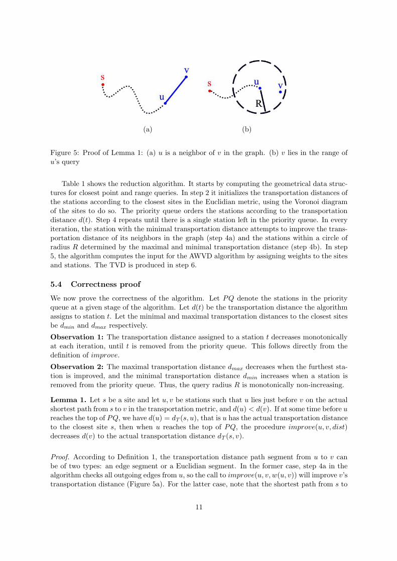
Figure 5: Proof of Lemma 1: (a) u is a neighbor of v in the graph. (b) v lies in the range ofu’s query
Table 1 shows the reduction algorithm. It starts by computing the geometrical data struc-tures for closest point and range queries. In step 2 it initializes the transportation distances ofthe stations according to the closest sites in the Euclidian metric, using the Voronoi diagramof the sites to do so. The priority queue orders the stations according to the transportationdistance d(t). Step 4 repeats until there is a single station left in the priority queue. In everyiteration, the station with the minimal transportation distance attempts to improve the trans-portation distance of its neighbors in the graph (step 4a) and the stations within a circle ofradius R determined by the maximal and minimal transportation distance (step 4b). In step5, the algorithm computes the input for the AWVD algorithm by assigning weights to the sitesand stations. The TVD is produced in step 6.
5.4 Correctness proof
We now prove the correctness of the algorithm. Let PQ denote the stations in the priorityqueue at a given stage of the algorithm. Let d(t) be the transportation distance the algorithmassigns to station t. Let the minimal and maximal transportation distances to the closest sitesbe dmin and dmax respectively.
Observation 1: The transportation distance assigned to a station t decreases monotonicallyat each iteration, until t is removed from the priority queue. This follows directly from thedefinition of improve.
Observation 2: The maximal transportation distance dmax decreases when the furthest sta-tion is improved, and the minimal transportation distance dmin increases when a station isremoved from the priority queue. Thus, the query radius R is monotonically non-increasing.
Lemma 1. Let s be a site and let u, v be stations such that u lies just before v on the actualshortest path from s to v in the transportation metric, and d(u) < d(v). If at some time before ureaches the top of PQ, we have d(u) = dT (s, u), that is u has the actual transportation distanceto the closest site s, then when u reaches the top of PQ, the procedure improve(u, v, dist)decreases d(v) to the actual transportation distance dT (s, v).
Proof. According to Definition 1, the transportation distance path segment from u to v canbe of two types: an edge segment or a Euclidian segment. In the former case, step 4a in thealgorithm checks all outgoing edges from u, so the call to improve(u, v, w(u, v)) will improve v’stransportation distance (Figure 5a). For the latter case, note that the shortest path from s to
11

v goes through u, therefore u’s transportation distance is smaller than the Euclidian distancefrom s to u, and the condition ambassador(u) in step 4b holds. The Euclidian improvementimplies that d(u) + dE(u, v) ≤ d(v), and by definition dmin ≤ d(u) ≤ d(v) ≤ dmax, thereforedE(u, v) ≤ d(v) − d(u) ≤ dmax − dmin = R, so v will be inside the range query in step 4b andthe call to improve(u, v, dE(u, v)) will update v’s transportation distance (Figure 5b).
Lemma 2. When a station t reaches the top of the priority queue PQ, the transportationdistance assigned to t equals the actual transportation distance from t to the set of its closestsites, that is: ∀s ∈ S(t) : d(t) = dT (s, t).
Proof. The proof is by induction on the number of stations deleted from PQ. Without lossof generality, assume that no two stations have the same transportation distance from theclosest site. Later we show how this assumption can be relaxed. Let d1, . . . , dk be the strictlymonotonically increasing transportation distances of the stations from their closest sites, andti be the corresponding station to the distance di, 1 ≤ i ≤ k. The induction hypothesis is thaton the ith iteration of step 4 of the algorithm, d(tj) = dj for all j < i. This holds for the firstiteration, because all the distances d(t) are initialized by the Euclidian distance to the closestsite, and d1 is the minimal d(t). We shall assume correctness for all i < m and prove for m.
Consider a shortest path from station tm to it’s closest site in the transportation metric,sm. If there are no stations on the path, then the path is a straight line and the initializationin step 2 of the algorithm assigns the proper value to d(tm). Otherwise, consider the stationti just before tm on the path. Since ti comes before tm on the path, it must be at least asclose to sm as tm, that is di ≤ dm. This implies i < m. By the induction hypothesis d(ti) = di
so ti has been removed from PQ. By Lemma 1, ti improves tm’s transportation distance andtherefore d(tm) = dm.
We now show that the sequence d1, . . . , dk need not be strictly monotonic. Consider thecase when the last station on the path has equal transportation distance to that of tm, that isdi = dm. Since the stations are unique, this can only happen when there is a zero weight edgebetween ti and tm. There are two possibilities to consider:
1. The zero weight edge between ti and tm improves tm’s transportation distance by go-ing through ti. This implies that d(ti) < d(tm) before the improvement, therefore thealgorithm will apply improve(ti, tm, 0) and assign the correct value to d(tm).
2. The algorithm assigns equal transportation distances to tm and ti prior to the improve-ment, that is d(tm) = d(ti). In this case ti may be removed from PQ after tm, but thedistance assigned to tm is still the correct distance, without the addition of ti to thepath.
Theorem 1. (Correctness of the reduction algorithm). Upon termination of the algorithm,all the stations t ∈ T have the following two properties:
1. The transportation distance assigned by the algorithm equals the actual transportationdistance to the set of t’s closest sites, that is ∀s ∈ S(t) : d(t) = dT (s, t).
2. The distance d(t) is smaller than the actual transportation distance to all the sites notin S(t), that is: ∀s /∈ S(t) : d(t) < dT (s, t).
12

s t1 t2 tk
Figure 6: Example of a worst-case input
Proof. Property 1 holds by the application of Lemma 2 with respect to the last iteration ofstep 4. For property 2, note that the improve procedure correctly updates the set of sites thatare associated with a station. When a better distance is achieved, the station is associatedonly with the new site. When an equal distance is discovered, the group of equidistant sites isupdated.
5.5 Complexity analysis
The computation of the Voronoi diagram and point location of S in step 1 takes O(n log n)time. Computing the range query data structure on T takes O(k log k) [1]. The initialization ofthe transportation distances in step 2 takes O(log n) for each station for a total of O(k log n).Using a Fibonacci heap for PQ, the amortized time for the primitive operations is as follows.Constructing the heap takes O(k), finding the minimum distance takes O(log k) and decreasingthe distance takes O(1). The algorithm also has to keep track of the maximal distance. Thiscan be achieved by another Fibonacci heap ordered in reverse. The while loop in step 4 isrepeated exactly k−1 times. Range queries take O(log k+c) time each, where c is the numberof stations returned. Note that every edge in the graph is checked for improvement only once,so this adds a total of O(e) improvement checks. The three dominant factors in the complexityare the number of edges (O(k2) in the worst case), the preprocessing and initialization steps(O((n + k) log n)), and the total number of stations in the range queries. We analyze the lastfactor next.
The key issue in the analysis of step 4 is the convergence of the query radius R. In theworst case, every query will result in all the stations being returned. Figure 6 gives an exampleof an input that causes this behavior. The minimal transportation distance dmin increases atevery iteration, while the maximal distance dmax is decreased, but the shortest transportationdistance to tk lies through all other stations, so the range query must return all the stationsthat remain in the priority queue. Thus O(k2) stations are returned for all the queries. Thisbrings the total complexity of the algorithm to O(k2 + (n + k) log n). Note that we omittedthe size of the graph from the complexity, as it is dominated by the O(k2) factor. In Section6 we show that in reality the worst case rarely happens, and the size of the graph becomesimportant.
5.6 Finding the shortest path
The following modification to the algorithm can be used to maintain information about theshortest path to the site. Each time that improve succeeds, the improved station stores thestation(s) from which the improvement was made. When the algorithm terminates, the pathto the site can be traced by walking backwards along these links. In the resulting Voronoidiagram, the AWVD cell of stations will be controlled by the closest site(s). A point locationquery that lies in a station cell can look up the closest path(s) by referring to the station.Point locations that lie on the cell of a site have a straight line shortest path to the site.
13

Figure 7: A suburban network with three suburbs
6 Transportation models
The worst-case scenario is not a good example for transportation networks. Real transportationnetworks are usually spread out to reach every part of the city, and are more dense in areaswith many sites. Next we discuss two realistic city transportation models and show how thealgorithm has a lower complexity on them.
6.1 Suburban networks (the cluster model)
The city suburbs are dense residential regions at some distance from the center of the cityand far apart from each other. The suburban network model, or cluster model, is a model ofthe transportation networks of clustered regions. Each cluster represents the transportationnetwork in a suburb. Transportation within the suburb is generally good, meaning that thereare many transportation lines in the suburb. Inter-suburb connection is sparse, restricted to asmall number of lines connecting the suburbs. Alternatively, the clusters may represent entirecities, each with its own independent transportation system, with a small number of inter-cityhighways and domestic flights. Figure 7 is an example of a suburban network. The squarenodes are the sites and the round nodes are stations.
In the following analysis, we assume without loss of generality that the clusters are discon-nected. The addition of inter-suburb lines can only lower the number of stations in the rangequeries, because successful improve operations reduce the values that determine the queryradius.
A cluster network is comprised of m groups of closely packed stations, each group far enoughfrom the others so as to not affect the transportation distance in them. Formally, let ki be thenumber of stations in the ith cluster Ti so that
∑mi=1
ki = k, kmax = maxi{ki}. Let dmax be thedistance of the furthest station from a site, and sep = min{dE(ti, tj)|ti ∈ Ti, tj ∈ Tj , i 6= j}, theminimal separation between clusters. We assume that dmax < sep, that is the shortest distancebetween any two stations on different clusters must be greater than the furthest distance from
14

Figure 8: A Uniform distribution of stations and sites
a station to its closest site.We analyze each cluster as if it were independent. The analysis is correct because the
cluster separation ensures that the maximal query radius around any station is containedwithin the station’s cluster. Note that this distinction is not necessary for the algorithm, andsuccessive stations from the top of the priority queue belong to different clusters. The worst-case input is that each cluster is a chain as in Figure 6. The sum of squares is smaller thanthe square of the sum, therefore
∑
i k2i ≤ k
kmaxk2
max and the total number of stations withinthe range queries is bounded by O(kkmax). The overall complexity of the reduction becomesO(kkmax + k log k + (n + k) log n + e).
Consider now two special cases of the cluster model:
1. In most cities, the size and number of the suburbs is proportional to the size of thecity: the larger the city the bigger and more numerous the suburbs are. Mathematicallythis means that the suburbs are of average size
√k, or kmax = Θ(
√k). This brings the
complexity of the algorithm down to O(k3/2 + (n + k) log n + e).
2. There are cities in which the suburbs are relatively small and isolated, and once theyare reached from the city center there is no need for internal transportation. We modelthis case with kmax = Θ(1). This reduces the complexity achieved further down toO(k log k + (n + k) log n + e).
6.2 Uniform spatial distribution model
There are cities in which there is no distinct center. The residential, commercial and industrialareas are intermixed and the transportation network must provide means to get everywhereas easily as possible. Figure 8 shows an example of a uniform distribution network.
This model assumes that within the largest query radius dmax from any station, there areO( k
n) neighboring stations on average. This means that there is no separation between thesites and the stations around them, so they are uniformly distributed.
15

The total number of stations returned in the queries is k times O( kn) so the overall com-
plexity is O(k2
n ). This brings the algorithm’s complexity to O( k2
n + (n + k) log n + e).Consider again two special cases:
1. The number of sites is significantly less then the number of stations. This is appropriatewhen the sites of interest are municipal establishments such as post offices or policestations. An appropriate relation between their numbers in this case is k = Θ(n2), sothe overall complexity is O(k3/2 + k log k + e).
2. The sites are intimately related to the stations, for example subway ticket stations or fastfood restaurants. This means that k = Θ(n), so the overall complexity is O(k log k + e).
7 Heuristics
In this section, we propose two heuristic approaches for reducing the radius of the range queryin each iteration.
The difference between the maximal and minimal transportation distance is a simple upperbound on the range of stations that can be improved by a Euclidian path. The actual range ofimprovable stations is influenced by the proximity of other stations and sites. In the sequel, weshow this range to be a complex shape composed of straight line segments, circular arcs, andhyperbolic segments, contained within the area of the upper bound range, and in many casesmuch smaller. In order to benefit from this observation, we propose heuristics that simplifythe range to enable efficient range queries with a reduced area. In Section 7.1 we describe theambassadors heuristic, which relies on the proximity of stations in the transportation graphto reduce the query range. In Section 7.2, we describe the Voronoi cell heuristic, which relieson the proximity of sites to eliminate stations that cannot be improved.
7.1 The ambassadors heuristic
When a station u improves a neighboring station v by a transportation line, v can potentiallypropagate this improvement to other stations in its vicinity. Since the graph edge weight isless than the Euclidian distance between the stations, it is faster to use the transportationline when going to a location near v. We call v an ambassador of u because v representsu within its zone of control. When u improves v’s transportation distance, v is still in thepriority queue, so the algorithm will eventually attempt improvements from v. Thus there isno need to attempt improvement from u to stations in v′s zone of control. The ambassador’szone of control is determined by the transportation distance bisector of u and v. A point p onthe bisector has the following property:
dE(u, p) = w(u, v) + dE(v, p)
This is the equation of an hyperbola, as discussed in Section 3. In the general case, the stationu may have several ambassadors. We determine the ambassadors’ zone of control by computingthe AWVD of the parent station and its ambassadors. We assign a zero weight to the parentstation and negative value of the edge weights for the ambassadors.
Since the ambassadors are bound to check the stations within their zone, the parent stationneed only check stations within the intersection of the query radius and its Voronoi cell. Whenthe parent station has a ambassadors, the intersection may compose of up to O(a) straightand hyperbolic segments. There is no efficient data structure for such range queries, so it mustbe simplified before the query is made.
16
Algorithm Ambassador-heuristic(t), returns: query radius.
1. Attempt all graph edge improvements from station t and insert the improved stations intoa list of ambassadors A
2. Assign weights:
• weight(t) := 0
• For all a ∈ A : weight(a) := −w(t, a)
3. Compute the AWVD of the parent station and its ambassadors
4. Compute the bounding region according to the Voronoi cell of t:
• If the cell is bounded:
(a) Find the furthest vertex of the cell and store the distance:R := maxv{dE(t, v)}, where v is a vertex of the cell
(b) If the new radius is smaller, use it in the range query:if R < R then return R
• else (the cell is unbounded), return the original query radius R
Table 2: The ambassadors heuristic algorithm.
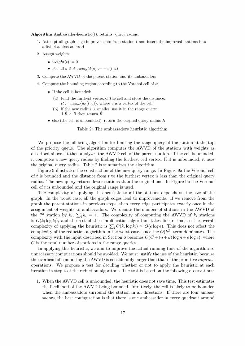
We propose the following algorithm for limiting the range query of the station at the topof the priority queue. The algorithm computes the AWVD of the stations with weights asdescribed above. It then analyzes the AWVD cell of the parent station. If the cell is bounded,it computes a new query radius by finding the furthest cell vertex. If it is unbounded, it usesthe original query radius. Table 2 is summarizes the algorithm.
Figure 9 illustrates the construction of the new query range. In Figure 9a the Voronoi cellof t is bounded and the distance from t to the furthest vertex is less than the original queryradius. The new query returns fewer stations than the original one. In Figure 9b the Voronoicell of t is unbounded and the original range is used.
The complexity of applying this heuristic to all the stations depends on the size of thegraph. In the worst case, all the graph edges lead to improvements. If we remove from thegraph the parent stations in previous steps, then every edge participates exactly once in theassignment of weights to ambassadors. We denote the number of stations in the AWVD ofthe ith station by ki,
∑
i ki = e. The complexity of computing the AWVD of ki stationsis O(ki log ki), and the rest of the simplification algorithm takes linear time, so the overallcomplexity of applying the heuristic is
∑
i O(ki log ki) ≤ O(e log e). This does not affect thecomplexity of the reduction algorithm in the worst case, since the O(k2) term dominates. Thecomplexity with the input described in Section 6 becomes O(C +(n+ k) log n+ e log e), whereC is the total number of stations in the range queries.
In applying this heuristic, we aim to improve the actual running time of the algorithm sounnecessary computations should be avoided. We must justify the use of the heuristic, becausethe overhead of computing the AWVD is considerably larger than that of the primitive improveoperations. We propose a test for deciding whether or not to apply the heuristic at eachiteration in step 4 of the reduction algorithm. The test is based on the following observations:
1. When the AWVD cell is unbounded, the heuristic does not save time. This test estimatesthe likelihood of the AWVD being bounded. Intuitively, the cell is likely to be boundedwhen the ambassadors surround the station in all directions. If there are four ambas-sadors, the best configuration is that there is one ambassador in every quadrant around
17

t
s
a4
a3
a1
a2
a5
t
a1
a2
a3
a4
(a) (b)
Figure 9: Application of the ambassadors heuristic. The filled region is the new query range.(a) the AWVD cell is bounded. The dashed lines denote the cell boundaries. The outer circledenotes the original query range. (b) the AWVD cell is unbounded
the station. In Figure 9b, the ambassadors a1, a2, a3, a4 are situated to the north andeast of the station t, thus no ambassadors cover the south and west sections. The generalcondition depends on the parameter α. We divide the unit circle around the station intoα cones. We apply the heuristic only if there is at least one ambassador in each of the αcones. A simpler alternative is to require that there are at least α ambassadors.
2. Even when the ambassadors properly surround the parent station, the parent’s Voronoicell may still be unbounded. The usefulness of the ambassadors depends on the weight ofthe edge that improved them: the smaller the weight, the larger the ambassador’s zoneof control. When the edge weight is close to the Euclidian distance between the parentand the ambassador, the ambassador is nearly useless. In Figure 9a, the ambassador a4
covers a very small section of the original circle. Based on this observation, we defineanother condition. Let β ∈ [0, 1) be an input factor parameter, let R be the currentquery radius, let t be the parent station and let a be an ambassador. Then we use theambassador a only if:
w(t, a) < βdE(t, a)
3. The heuristic is only useful if the range query returns a large number of stations. In thefinal iterations of the reduction algorithm, the query radius is relatively small and thereare few stations left. Therefore it would be better to use the circular range queries withoutapplying the heuristic. We can estimate the usefulness of the heuristic by evaluating afunction of the number of ambassadors ki, the current query radius R, the average queryradius when the heuristic is applied R, and the density of the stations in the previousrange queries ρ. We shall use the input parameter γ as an estimate to the overhead ofthe AWVD algorithm. The condition we propose is:
γki log ki < ρπ(R − R)2
18

We compute the density ρ according to the results of the last query. Let c be the numberof stations returned in the last query, and let A be the previous query area, then ρ = c
A .The density in the first iteration is determined by the area of the bounding box of thestations and the total number of stations.
The test can consist of any subset of the above conditions. All the conditions add only aconstant number of arithmetic operations per ambassador. If the third condition is used, thepredicate can be skipped altogether after the condition failed φ times, where φ is an inputinteger.
7.2 Voronoi cell heuristic
The ambassadors heuristic exploits the proximity of neighboring stations in order to limit thequery range. Similarly, the Voronoi cell heuristic exploits the proximity of sites to reduce thequery range.
Consider station t1 in Figure 10. Assume without loss of generality that s1 is closestto t1 in transportation distance and that the distance is dT (t1, s1) = 0. In order for t1 toimprove another station, the station must be closer to t1 than to any other site. Thus, theimproved station must lie within the Voronoi cell of t1 in order to be improved. The dashedlines in Figure 10 bound the standard Voronoi cell of t1 with the point set S ∪ t1. When thetransportation distance is greater than zero, the Voronoi cell is that of the AWVD where thesites have zero weight, and the station a negative weight equal to its transportation distance.The dotted curve around station t2 in Figure 10 bounds the AWVD cell of S ∪ t2. The dashedlines containing the AWVD cell are the boundary of the standard Voronoi cell of t2.
This observation leads to the following heuristic approach. We compute the distance fromthe improving station to the vertices of its standard Voronoi cell. Denote the maximal distanceas R, and the difference between the largest and smallest transportation distances as R. Thenthe radius of the range query is taken as min(R, R). The shaded circle in Figure 10 is thequery radius of the station t1.
In order to compute the Voronoi cell of t, we use the Delaunay graph of the set of sites S,which was constructed in the preprocessing step. We insert t into the Delaunay graph withan efficient dynamic triangulation algorithm (see for example de Berg [5]). There is no needto construct the Voronoi cell explicitly. Instead, the distance of the vertices from the station tis computed as the radius of the circle defined by t and two consecutive neighbors of t in theDelaunay graph.
The complexity of applying this heuristic depends on the placement of stations withinthe Voronoi cells of the sites. On average, the Voronoi cell in which a station resides hassix vertices, so it takes constant time to locally re-triangulate the cell, for a total of O(k)operations. In the worst case all the stations reside in a single Voronoi cell with O(n) vertices,resulting in O(kn log n) operations. It is therefore important to apply the heuristic only whenthe reduction in the query radius justifies it. As in Section 7.1, we propose a simple test fordetermining whether to apply the heuristic. Let ρ be the density of the stations in the previousquery, let d be the average number of edges in a cell of the Voronoi diagram of the set of sitesS (without computing, we can assign d = 6), let R be the average query radius when theheuristic is applied, and let γ be the test overhead parameter. Then the condition for applyingthe heuristic is:
γd < ρπ(R − R)2
When this test fails φ times, the algorithm skips the test and does not apply the heuristic untilit terminates.
19

t1
t2s1
Figure 10: Voronoi cell heuristic
Observe now that we defined the actual range in which improvable stations possibly exist.It is the intersection of the circular range with the additively weighted Voronoi cell of thestation with respect to its ambassadors, and the additively weighted Voronoi cell of the stationwith respect to its neighboring sites. The region is non-convex and consists of straight linesegments (from the bisectors of zero weight ambassadors or from the Voronoi cell of the stationwhen its transportation distance is zero), circular arcs (from the circular range query) andhyperbolic segments (from the bisectors when the weight is non-zero). The overhead involvedin computing such a range query surpasses the gain of using it, therefore it must be simplifiedas described above.
8 Extensions
Travel in public transportation networks often involves changing lines several times beforereaching the destination. Moving from one line to another takes time, and it is this additionalcost to the shortest paths that we model next.
In general, there are three types of additional time costs: access, connection, and waiting.Access time is the time it takes to enter or leave the subway tunnels or train stations. Often,the distance from the street to the subway station is significant. Connection time is the time ittakes to switch between transportation lines. The distance between different lines in the samestation is also significant. Waiting time is the average time spent waiting for the transportationto arrive. The waiting period depends on the hour of day and the frequency of the line. Manysubway networks publish the average waiting times for the different lines.
We model these features as follows. Access time is a property of the stations: the largerthe station the longer the average access time to its transportation lines. For each stationt ∈ T , we denote the access time by access(t). Whenever the path involves entering orleaving t, we add access(t) to the cost of the path. We modify the reduction algorithm (Table1) to reflect these changes. In step 4b the cost of the improvement attempt is access(t) +dE(t, u) + access(u), that is the cost of leaving the current station t, going from t to u by
20

foot, and entering the transportation network at u. Notice that this also reduces the radiusof improvable stations. We can update the radius in step 4 by calculating R = dmax − dmin −access(t) − minu∈T\{t}{access(u)}.
The waiting time is a property of the transportation lines, as each line has its own frequency.Connection time depends on whether the path switches lines and on the size of the connectingstation. We associate with each graph edge e = (u, v) the line number line(u, v), and with eachline number l the waiting time wait(l). When the path includes a graph edge (u, v), we add thewaiting time wait(line(u, v)) to its cost. When the path includes two consecutive edges withdifferent line numbers, we add the connection cost of the connecting station. The most realisticmodel would assign a connection cost to each pair of edges connect(ei, ej), ei, ej ∈ E, becauseeach station has different access paths for each line. This however requires O(e2) = O(k4) spacein the worst case. An alternative is to assign a cost to the connecting station, connect(t), whichdepends on the size of the station and the average distance between the different lines. Wemodify the station data structure so that it contains the set of numbers of the lines connectingit to its closest sites. For a station t, we denote this set by L(t). We modify the improveprocedure to maintain L(t), and modify step 4a of the reduction algorithm as follows:
Let u be the graph-neighbor of the current station t, and let w(t, u) be the cost of the
connecting line.
• if L(t) = ∅ (t was reached by foot) then the cost of the improvement attempt is
wait(t, u) + w(t, u)
• else if line(t, u) ∈ L(t) (no need to switch lines) then the cost is w(t, u)
• else (line(t, u) /∈ L(t), switching lines) the cost is connect(t)+wait(line(t, u))+w(t, u)
The modified algorithm computes the reduction from TVD to AWVD when the inputcontains information about the access, connection and waiting times of the network. Thecomplexity of the algorithm remains the same because the modification of step 4 adds aconstant number of branching operations per iteration, and the total number of operations formaintenance and membership testing in the sets L(t) is linear in e.
9 Implementation and results
In this section we describe the implementation of the algorithm and present the results ofexperiments on five input models with variable number of sites, stations and edges.
The goals of the implementation are:
• To demonstrate that the proposed algorithm is practical.
• To compare the performance of the proposed input sensitive algorithm to that of thebasic algorithm.
• To quantify the efficacy of the proposed heuristics on a variety of inputs.
9.1 Implementation details
The algorithm was implemented using the Library of Efficient Data structures and Algorithms(LEDA). Specifically, we used the Delaunay tessellation, range query and graph data struc-tures. The priority queue was implemented using the Standard Template Library (STL) mul-timap (a Red Black tree) instead of a Fibonacci heap because of the need to keep track of the
21
maximal distance station (the LEDA p queue class does not support increase key operations).This adds an O(log k) complexity for each successful improve, theoretically increasing theworst-case complexity to O(k2 log k + (n + k) log n + e). In addition, the LEDA circular rangequery algorithm does not guarantee the optimal O(log k + c) running time. Nevertheless, ex-periments show that performance is not affected asymptotically, because there are rarely morethan O(k) successful improvements on realistic inputs. We ran the experiments on an AMDAthlon 800 MHz processor with 128 MB of memory, operating on Windows 2000.
We used the following random generators of input in our experiments:
1. Random input. We used LEDA’s point generator to generate sites with a uniform dis-tribution inside a disc of radius r. Within the disc, we generated random positions forthe transportation graph nodes. The graph edges were randomly chosen for e pairs ofstations.
2. Suburban network input. We created clusters by generating groups of localized pointsseparated from each other to satisfy the cluster condition. At least one cluster wascreated with kmax stations (an input parameter). Within the clusters, the sites andstations were generated randomly.
3. Uniform spatial distribution. The algorithm randomly generates stations inside a squareof length l, and the square is divided into sub-squares, each associated with a singlerandomly placed site. This input ensures that the average number of stations in rangequeries is close to k
n (within a small fraction from that number).
4. Extended Euclidian Minimum Spanning Tree (EEMST). The Euclidian Minimum Span-ning Tree (EMST) is a tree that spans all the nodes and minimizes the total Euclidianlength of the graph edges. It is used by network planners to minimize the cost of con-structing and maintaining the network, and thus it is a good model for transportationnetworks. The EMST is a subgraph of the Delaunay tessellation graph [12]. The EEMSTis constructed from the EMST by including additional edges from the Delaunay graph.When the desired input has k stations and e transportation lines, we connect each stationto its e
k closest neighbors, not counting stations that are already connected.
5. Old city model. Studies of old city development show that most cities start in one denselypopulated area, and expand in concentric circles of increasing radii. We simulate thisevolution by 10 stages of randomized input, each stage placing sites and stations withina disc of increasing radius, with a uniform distribution. The result is a densely populatedcenter that becomes sparser as the radius increases. We used the density parameter ρ inas follows: if k is the total number of desired stations, then ρk stations are generated inthe first stage. In the second stage ρ(k − ρk) stations are generated, and so on until thefinal stage, where all the remaining stations are generated within a disc of the maximalradius. Thus, if ρ = 0 the density is uniform, and if ρ = 1 then all the stations areconcentrated in the innermost circle. The density parameter ρ of Paris is approximately0.05.
All these models use the transportation speed parameter s ∈ [0, 1] when assigning weightsto the transportation lines. Denote the Euclidian distance between a pair of neighboringstations by d. Then the weight is generated randomly in the interval [0, sd].
22

14
21
18
17
20
17 19
9
11
32
12
10
14
96
60
48
37
90
23
58
59
81
77
40
������������� �� ����
� ��� ���������� �
� � � � "!$# �$% �$� &'�
(*)+&'�$)+� # �
��&�&)+&'�$� !�, � )-&. , /$0 )'12���'�
. , /-3 �� % � �# ��4�)-�% �5��$)-�76��98
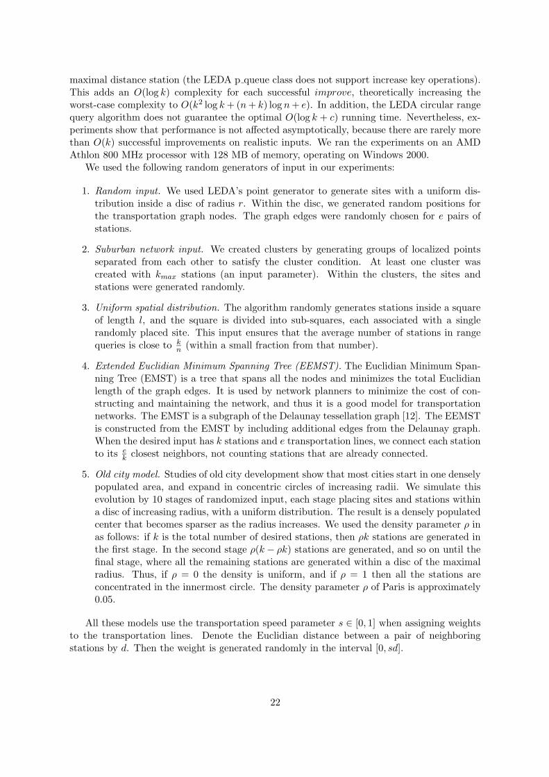
Figure 11: Transportation distance to Paris churches. The weight of the Metro lines is displayedalongside the edges. The number inside the station nodes denotes the transportation distanceto the closest church. Note that many stations are closest to the Madeleine church, even thoughthey are closer in Euclidian distance to other churches.
9.2 Results
Both the basic algorithm and our algorithm (hereafter input sensitive algorithm) check all theedges for possible improvement in the transportation distance, so the difference between themlies in the number of Euclidian improvements tried. All the experiments were done on randominput of the five models above. Complexity and running time values are the average of 40runs on input with the same parameters. We only compare the running times of the reductionalgorithms. The computation of the AWVD from the reduction input is the same on bothalgorithms.
We compared the theoretical bounds on the number of stations within the range querieswith the number calls to the primitive improve function. This number depends largely on theconvergence of the query radius and the density of sites and stations. The experiments showthat the measured complexity is significantly better than the theoretical bounds suggest. Thisis because the input in reality is seldom worst case.
9.2.1 Transportation Voronoi Diagram of Paris
We ran the algorithm on the Paris metro and tourist sites. Figure 1 shows the the ParisMetro stations and lines (dots and solid lines), the tourist sites (squares) and the shortesttransportation distance relation from Metro stations to tourist sites (dotted lines). Figure11 shows a detail of the result in the Champes Elysees area. The input comprises of 325Metro stations with 352 lines and 78 tourist sites. The running time of the algorithm was 160milliseconds.
23

0 1000 2000 3000 4000 5000 6000 7000 8000 90000
1
2
3
4
5
6
7x 10⁴
:+;+<�='>�?A@+BDC E F�E G @$:�C
H IJJK JLMK NOP NKQQK ROSTJU RV
basic TVD input sensitive TVD
0 1000 2000 3000 4000 5000 6000 7000 80000
1000
2000
3000
4000
5000
6000
7000
W-X-Y[Z�\2]D^$_a` b c2b d ^�W�`
e fggh gijh klm khnnh olpqgr os
tatauwv+xzy ` {}|�~ �tatauwv+xzy ` {}|�~ �+�` X$Z+X-] Z�c2W y ` {�|�~ �X$W+d _ ^�] Y y ` {}|�~ �+�] c2W��$^�Y y ` {}|7~ �
(a) basic vs. input sensitive algorithm (b) input sensitive algorithm with various inputs
0 2000 4000 6000 8000 10000 12000 14000 16000 180000
0.5
1
1.5
2
2.5
3 x 10⁵
�-�-�[���2�D�-�� � �2� � �����
� ���� ���� ��� ����� ������ ��
����� � �z� �¡� �$¢+�$�� ����� � � � £��z� �¡ ���� ���������¤��¥ ¥-¦��2�-� � � � �z� �¡
100 101 102 103 104 105102
103
104
105
106
107
§-¨-©«ª�¬�D®-¯a° ± ² ¬�°
³ ´µ¶ ·¸¹º »¼¼ ·µ½¾
± §$¿+¨-²'°7¬�§�° ± ² ± À�¬zÁDÂ�Ã"Ĥ®�©«¿�Å ¬2Æ+± ² Ç
(c) with Voronoi cell heuristic (d) Varying number of sites
Figure 12: Experimental results
24

9.2.2 Comparison between the algorithms
Figure 12a shows the running time of the basic versus the input sensitive algorithm. The inputmodel used here is the EEMST with speed parameter s = 1/2. We kept the ratio of numberof sites, stations and edges as a constant 1:4:16 respectively, and varied the input size fromk = 23 to k = 213. While the basic algorithm exhibits the expected quadratic dependency onk, the input sensitive algorithm shows a nearly linear dependency. At k = 213 our algorithmis one order of magnitude faster than the basic algorithm.
9.2.3 Running time on different input models
Figure 12b shows the running times of the extended algorithm with five different input modelswith a ratio of 1:4:16 on sites, stations and edges, respectively.
The EEMST input with s = 1/2 incurs the worst running time. Increasing the speedof the transportation to s = 1/20 results in improvement by edges that significantly reducethe transportation distances of the stations, thus decreasing the range query radius and thecomplexity of the reduction.
The suburban network input was taken with kmax =√
k. The predicted complexity hasan O(k3/2) dependency on k. The experiment shows that in reality the complexity is lower,because the input is not worst case as assumed in the analysis.
The uniform spatial distribution and the random input have the lowest running times. InSection 6.2 we predicted that when n = O(k), the number of stations in the range queriesis linear in k, and the complexity is dominated by the preprocessing step. The experimentshows that this prediction holds. There is another factor that reduces the running time on theuniform input: the number of stations that remain unimproved. This factor is the main reasonthat the random input has the lowest running time. When the edges are chosen randomly andthe weight is proportional to the distance between the stations, the average edge weight ishigher and thus less stations can be improved by a transportation line. When the stationremains unimproved, the algorithm skips the Euclidian improvement step, thus saving time.
9.2.4 Application of the Voronoi cell heuristic
The old city model produces input with a region of high density of stations and sites. Thisresults in a high number of stations returned from range queries. Figure 12c shows the runningtime of the basic algorithm and the extended algorithm with and without application of theVoronoi cell heuristic. Once again, the ratio of sites, stations and edges is 1:4:16, respectively.We used an unrealistically high density value ρ = 0.15 in order to stress the results.
The basic algorithm is not sensitive to the input, and has the same quadratic runningtime. The input sensitive algorithm, while significantly better than the basic algorithm, has areduced performance with this input. The application of the Voronoi cell heuristic improves theperformance, reducing the running time to values slightly higher than the values on uniformdensity with EEMST.
We tested the heuristic on various inputs in order to see if the overhead of computing theVoronoi cell costs in performance. The heuristic test we propose with overhead factor γ = 2ensures that the algorithm runs on all inputs at least as fast as without applying the heuristic,usually faster.
We did not implement the ambassadors heuristic because we lack of an efficient implemen-tation of the AWVD algorithm.
25

9.2.5 Fixed number of stations
The number of sites is a major factor in determining the radius of the range queries. The fewersites there are, the larger the distances from stations to sites get. These distances determinethe query radius.
We conducted a series of experiments with a fixed number of stations and sites, k =4096, e = 8192. We increased the number of sites from 23 to 215 and measured the number ofcalls to the improve procedure as a measure of the complexity. The results are shown on alogarithmic scale in Figure 12d. The number of improvement attempts is nearly quadratic ink in the range 1 < s < 64. It is sub-quadratic in the range 64 < s < 512, and approximatelylinear afterwards. Note that these experiments were made without the application of anyheuristic. The Voronoi cell heuristic significantly improves the performance when the numberof sites is O(
√k) or higher, and the ambassadors heuristic helps when there are numerous fast
transportation lines.
10 Conclusion and future work
The Transportation Voronoi Diagram (TVD) is a natural combination of geometry and graphtheory. It generalizes the standard Voronoi diagram to the transportation metric. This paperis the first detailed analysis of the problem and the properties of TVDs. Given a transportationnetwork and a set of sites, the TVD encapsulates information about closest sites and distancesin the transportation metric.
We developed an input sensitive algorithm for the reduction from TVD to AWVD. Forinput with n sites, k stations with e transportation lines, the reduction algorithm has a worst-case complexity of O(k2 + (n + k) log n). We showed that for realistic transportation networkmodels the algorithm has a complexity of O(k log k + (n + k) log n + e). Our experimentsshow that on random city transportation networks the complexity, which is lower than thelatter bound, is also characteristic of almost all inputs. This improves upon the algorithm byAichholzer et al. [3], which has the same worst complexity on all inputs and does not take intoaccount the size of the transportation graph or the geometrical properties of the stations andthe sites, as our algorithm does.
An outstanding open problem is to determine if the worst-case quadratic complexity is thelower bound of the reduction to AWVD.
Terrains with obstacles are a natural extension to consider next. In reality, there areimpassable obstacles such as rivers, large buildings or private areas. We can model these aspolygonal obstacles and combine the transportation metric with the geodesic distance metric.Wang and Tsin describe an algorithm for finding the constrained and weighted Voronoi diagramin [15]. Using an extended reduction algorithm to compute the weights with the geodesicdistance, we can construct the Geodesic TVD.
Transportation networks are very dynamic: routes close for repair, new lines open, rushhour traffic increases the weights of main routes, and unscheduled delays affect waiting times.Local changes in the network may entail changes in the entire network shortest paths map.Future work will explore how these changes can be computed efficiently.
11 Acknowledgements
The author would like to thank Franz Aurenhammer for the help and support in starting theresearch. This research was supported in part by a grant from the Ministry of Science and
26

Technology, Israel.
References
[1] A. Aggarwal, M. Hansen, and T. Leighton. Solving query-retrieval problems by compact-ing Voronoi diagrams. In Proc. 22nd annu. ACM symp. theory comp., pages 331–340,1990.
[2] O. Aichholzer, F. Aurenhammer, D. Z. Chen, D. T. Lee, and E. Papadopoulou. SkewVoronoi diagrams. International Journal of Computational Geometry and Applications,9(3):235–247, 1999.
[3] O. Aichholzer, F. Aurenhammer, and B. Palop. Quickest paths, straight skeletons, andthe city Voronoi diagram. In Proc. of the 18th an. sym. on Computational Geometry,pages 151–159, 2002.
[4] F. Aurenhammer and R. Klein. Voronoi Diagrams. In J.-R. Sack and J. Urrutia, editors,Handbook of Computational Geometry, pages 201–290. Elsevier Science Publishers B.V.North-Holland, Amsterdam, 2000. Edited by J-R. Sack, J. Urrutia.
[5] M. de Berg, M. van Kreveld, M. Overmars, and O. Schwarzkopf. Computational Geometryalgorithms and applications. Springer, 2000.
[6] S. Fortune. A sweepline algorithm for Voronoi diagrams. Algorithmica, 2(2):153–174,1987.
[7] L. Gewali, A. Meng, J. S. B. Mitchell, and S. Ntafos. Path planning in 0/1/∞ weightedregions with applications. ORSA Journal of Computing, 2(3):253–272, 1990.
[8] J. Hershberger and S. Suri. An optimal algorithm for Euclidean shortest paths in theplane. SIAM J. Comput., 28(6):2215–2256, 1999.
[9] M. Karavelas and M. Yvinec. Dynamic additively weighted Voronoi diagrams in 2D.Technical report, INRIA Sophia-Antipolis, 2002.
[10] J. Mitchell and C. Papadimitriou. The weighted region problem: finding shortest pathsthrough a weighted planar subdivision. Journal of the ACM, (38):18–73, 1991.
[11] J. S. B. Mitchell. Geometric shortest paths and network optimization. In J.-R. Sackand J. Urrutia, editors, Handbook of Computational Geometry, pages 633–701. ElsevierScience Publishers B.V. North-Holland, Amsterdam, 2000.
[12] A. Okabe, B. Boots, and K. Sugihara. Spatial Tessellations: Concepts and Applicationsof Voronoi Diagrams. John Wiley and Sons, Inc., New York, New York, 1992.
[13] N. C. Rowe. Roads, rivers, and obstacles: optimal two-dimensional path planning aroundlinear features for a mobile agent. Internat. J. Robot. Res., 9:67–73, 1990.
[14] M. Sharir. Intersection and closest pair problems for a set of planar discs. SIAM Journalof computing, 14(2):448–468, 1985.
[15] C. A. Wang and Y. H. Tsin. Finding constrained and weighted Voronoi diagrams in theplane. Computational Geometry Theory and Applications, 10:89–104, 1998.
27

[16] H. Yomono. The Voronoi diagram on a network. Technical report, Nippon Systems Co,Tokyo, 1991. In Japanese.
28
Top Related