


Languages
Pages
Legal


TRADE MODELS AND MACROECONOMICS
By
Ray C. Fair
December 2019
COWLES FOUNDATION DISCUSSION PAPER NO. 2214
COWLES FOUNDATION FOR RESEARCH IN ECONOMICS YALE UNIVERSITY
Box 208281 New Haven, Connecticut 06520-8281
http://cowles.yale.edu/

Trade Models and MacroeconomicsRay C. Fair∗
December 2019
Abstract
This paper discusses some macro links that are missing from trade models.A multicountry macroeconometric model is used to analyze the effects onthe United States of increased import competition from China, an experimentthat is common in the recent trade literature. In the macro story a fall inChinese export prices is stimulative. Domestic prices fall, which increasesreal wage rates and real wealth, which increases household expenditures. Inaddition, the Fed may lower the interest rate because of the lower prices,which is stimulative. Trade models do not have these channels, and theylikely overestimate the negative effects or underestimate the positive effectson total output and employment from increased Chinese import competition.They lack some important aggregate demand channels, which are not likelysecond order.
1 Introduction
Macroeconomics does not play much of a role in trade models. This paper con-
siders whether the role should be larger. When computing, say, the effects of a
productivity increase in China on the U.S. economy, how much is lost if macro
effects are ignored? There are a number of recent trade papers analyzing the effects
of import competition from China on the United States. Autor, Dorn, and Hanson
∗Cowles Foundation, Department of Economics, Yale University, New Haven, CT 06520-8281.e-mail: [email protected]; website: fairmodel.econ.yale.edu. I am indebted to Lorenzo Caliendofor helpful discussions about his model and for supplying me with extra results.

(2013) (ADH) find that exposure to Chinese import competition in U.S. local labor
markets has a negative effect on manufacturing employment in the local market
and on nominal wages outside the manufacturing sector. They find large effects.
For example, they find that rising exposure to Chinese import competition explains
21 percent of the decline in U.S. manufacturing employment between 1990 and
2007 (p. 2140). They note in the conclusion (p. 2159) that theory suggests that
trade with China should yield positive overall gains for the U.S. economy. Total
effects on the economy are not estimated in their paper. Import prices are exoge-
nous in their model, which rules out estimating overall effects. But given the large
estimated losses, there must be large gains elsewhere.
Pierce and Schott (2016) (PS) find negative U.S. manufacturing employment
effects after the United States granted Permanent Normal Trade Relations (PNTR)
to China in 2000. They do not attempt to estimate the overall effects on the U.S.
economy from this change. Acemoglu, Autor, Dorn, Hanson, and Price (2016)
(AADHP) find very large effects from rising Chinese import competition. They
estimate job losses from this competition over 1999–2011 of between 2.0 and
2.4 million. This estimate includes what they call “aggregate demand spillovers”
(p.S̃183) from the initial shocks. They view any possible positive aggregate demand
effects from a lower aggregate price level as second-order and do not consider this
possible channel (p. S149, footnote 14). Their analysis thus implies large losses
from trade.
Caliendo, Dvorkin, and Parro (2019) (CDP) are also interested in the effects
on the U.S. economy of increased Chinese import competition. Their approach is
quite different from that of the papers just mentioned. They construct a general
equilibrium model of 22 sectors, 38 countries, and 50 U.S. states for the 2000–2007
period. They use the model to estimate what the U.S. economy would have been
like had there been no China shock—no increase in Chinese productivity. They
also find large negative effects on U.S. manufacturing employment from the China
shock. However, the net effect on a measure of U.S. welfare in their model and on
2

U.S. GDP is slightly positive. The gains in some sectors slightly offset the losses
in others. As extensive as this model is, it does not include some of the macro
effects discussed below. More will be said about this later.
The macro model used in this paper is my multicountry econometric model,
denoted the “MC model,” discussed next. The model is used to estimate the
effects of lower Chinese export prices on the world economy, particularly on the
U.S. economy. The aggregate effects on the United States are positive—aggregate
output and employment are higher—and the channels that lead to these effects
differ somewhat from those in trade models. They arise through real income, real
wealth, interest rate, and exchange rate effects.
Section 2 outlines the MC model and the methodology behind it. A China shock
is then analyzed in Section 3, first qualitatively and then quantitatively. Section 4
discusses some of the differences between the MC model and trade models.
2 The MC Model
The latest version of the MC model is in a document on my website, “Macroe-
conometric Modeling: 2018,” which will be abbreviated “MM”. Most of my past
macro research, including the empirical results, is in MM. It includes chapters
on methodology, econometric techniques, numerical procedures, theory, empirical
specifications, testing, and results. The results in my previous macro papers have
been updated through 2017 data, which provides a way of examining the sensitivity
of the original results to the use of additional data.
The model of the United States is a subset of the MC model, and it will be
denoted the “US model.” The MC model of all the other countries will be denoted
the “ROW model.” There are 37 countries in the MC model for which stochastic
equations are estimated. There are 25 stochastic equations for the United States
and up to 10 each for the other countries. The total number of stochastic equations
is 232, and the total number of estimated coefficients in these equations is about
3

1,000. In addition, there are 797 bilateral trade share equations estimated, so the
total number of stochastic equations is 1,029. The total number of endogenous
and exogenous variables, not counting various transformations of the variables and
the trade share variables, is about 1,700. Trade share data were collected for 56
countries. Counting an “all other” category, the trade share matrix is 57× 57.
The estimation periods begin in 1954 for the United States and as soon after
1960 as data permit for the other countries. The periods for the trade share equa-
tions begin in 1976:1 or later. The periods end as late as 2017:4. The estimation
technique is two stage least squares (2SLS) except when there are too few observa-
tions to make the technique practical, where ordinary least squares (OLS) is used.
OLS is used to estimate the trade share equations. The estimation accounts for
possible serial correlation of the error terms. The variables used for the first stage
regressors for a country are the main predetermined variables in the model for the
country.
There is a mixture of quarterly and annual data in the model. Quarterly equa-
tions are estimated for 14 countries, and annual equations are estimated for the
remaining 23. However, all the trade share equations are quarterly. There are
quarterly data on the variables that feed into the trade share calculations, namely
the price of exports per country and the total value of imports per country.
It is too much to explain the model in one paper, and I will rely on MM as the
reference. Think of MM as the appendix to this paper. In what follows the relevant
sections in MM will be put in brackets.
The modeling methodology is discussed next, followed by outlines of the US
and ROW models. The focus in this discussion is on features of the model that
pertain to the China experiment.
4

The Cowles Commission (CC) Approach
What I call the CC approach [MM, 1.1] is the following. Theory is used to guide the
choice of left-hand-side and right-hand-side variables for the stochastic equations
in a model, and the resulting equations are estimated using a consistent estimation
technique like 2SLS. Sometimes restrictions are imposed on the coefficients in
an equation, and the equation is then estimated with these restrictions imposed.
It is generally not the case that all the coefficients in a stochastic equation are
chosen ahead of time and thus no estimation done. In this sense the methodology
is empirically driven and the data rule. Some argue that models specified using the
CC approach are ad hoc, but this is not the case. Behavioral equations of economic
agents are postulated and estimated. The CC approach has the advantage of using
theory while keeping close to what the data say.
Typical theories for these models are that households behave by maximizing
expected utility and that firms behave by maximizing expected profits. The theory
that has been used to guide the specification of the MC model is discussed in [MM,
3.1, 3.2]. In the process of using a theory to guide the specification of an equation
to be estimated there can be much back and forth movement between specification
and estimation. If, for example, a variable or set of variables is not significant
or a coefficient estimate is of the wrong expected sign, one may go back to the
specification for possible changes. Because of this, there is always a danger of data
mining—of finding a statistically significant relationship that is in fact spurious.
Testing for misspecification is thus (or should be) an important component of the
methodology. There are generally from a theory many exclusion restrictions for
each stochastic equation, and so identification is rarely a problem—at least based
on the theory used.
The transition from theory to empirical specifications is not always straightfor-
ward. The quality of the data is never as good as one might like, so compromises
have to be made. Also, extra assumptions usually have to be made for the em-
pirical specifications, in particular about unobserved variables like expectations
5

and about dynamics. There usually is, in other words, considerable “theorizing”
involved in this transition process. In many cases future expectations of a variable
are assumed to be adaptive—to depend on a few lagged values of the variable itself,
and in many cases this is handled by simply adding lagged variables to the equa-
tion being estimated. When this is done, it is generally not possible to distinguish
partial adjustment effects from expectation effects—both lead to lagged variables
being part of the set of explanatory variables [MM, 1.2].
This methodology differs substantially from that behind the specification of
DSGE models. For these models the theory is much tighter (more restrictive),
rational expectations is assumed, and there is considerable calibration. These
differences are discussed in Fair (2019), which also summarizes some of the main
results from my macroeconmetric modeling—empirical points that should be taken
into account in constructing macro models.
The US Model
The following is a brief discussion of the main estimated equations. All the ex-
penditure equations are in real terms. The following discussion of the explanatory
variables ignores possible lagged dependent variables. A complete discussion of
the US model, both the theory and the empirical specifications, is in [MM, 3.2,
3.6].
There are four expenditure equations of the household sector—consumption of
services, nondurables, and durables, and housing investment—and the key explana-
tory variables are disposable income, interest rates, lagged wealth, age distribution
variables, and lagged stocks for the durable and housing equations. There are four
household labor supply equations—the labor force of males 25-54, females 25-54,
all others 16+, and the number of people holding more than one job. The key
explanatory variables are the real wage rate, lagged wealth, and the unemployment
rate. Lagged wealth has a negative effect on labor supply—a negative income
6

effect. The unemployment rate has a negative effect and is picking up discouraged
worker effects.
There are six important stochastic equations of the firm sector. Plant and
equipment investment depends on output, lagged excess capital, and interest rates.
Production depends on sales and the lagged stock of inventories. The demand
for jobs and hours per job depend on output and lagged excess labor. In the two
price and wage rate equations the price level depends on the wage rate, the import
price index, and the unemployment rate. The wage rate and import price index are
cost variables, and the unemployment rate is the demand variable. The wage rate
depends on productivity and the price level. The fact that the import price index is
an explanatory variable in the domestic price equation—the equation determining
the price level of the firm sector—is important for the present analysis. The index
is highly significant in the equation and also in almost all of the domestic price
equations for the other countries. [MM, 3.6.4, 3.7.2] If, say, import prices fall, the
aggregate estimates are picking up the behavior of firms lowering their prices to
compete with the lower prices of imported goods. Also, prices of inputs that are
imported may be lower, which may lead to lower domestic output prices.
There is an estimated interest rate rule of the Fed. The short term interest rate
depends on inflation and the unemployment rate. The Fed is estimated to “lean
against the wind.” Long term interest rates are affected by the short term rate
through estimated term structure equations.
There is an estimated import equation, where the level of imports depends
on disposable income, lagged wealth, and the domestic price level relative to the
import price index.
A key property of the US model from the perspective of this paper is the effect
on the economy of a change in the import price index (PM ), ignoring for now
rest-of-world effects. Let PF denote the price level for the firm sector. As just
noted, a decrease in PM leads to a decrease in PF since PM is an explanatory
variable in the firm price equation. As an empirical matter PF does not fall
7

as much as PM does, and so PF/PM rises, which increases the demand for
imports through the estimated import equation. The price and wage equations
are such that a fall in PF does not result in as large a fall in the nominal wage
rate (the nominal wage rate lags the price level), and so the real wage rate rises.
This leads to an increase in real disposable income, which has a positive effect
on household expenditures. In addition, the fall in PF leads to a rise in real
wealth, which also has a positive effect on household expenditures. The increase
in household expenditures is expansionary on total output, and the increase in
imports is contractionary. The net effect in the US model is positive, and so a
decrease in PM leads to an increase in aggregate output and then to increases in
jobs and hours per job from the firm-sector equations. The unemployment rate is
lower. The effect on the short term interest rate set by the Fed is ambiguous since
inflation is lower and the unemployment rate is lower.
The ROW Model
There are estimated models for 36 other countries. These models are not as detailed
as the US model. All the countries are linked by estimated trade share equations.
Table 1 lists the main variables in each country’s model and the main explanatory
variables in the estimated equations. If there is no subscript on a variable, it is
for country i. If there is a subscript j, this represents all the other countries in the
model. The expenditure variables are real and are in units of 2010 local currency
(lc). A variable with a $ at the end is in units of 2010 U.S. dollars. E is the
exchange rate, lc/$, and so an increase in E is a depreciation of the country’s
currency relative to the U.S. dollar. E10 is the exchange rate in 2010. A variable
like (E10/E)PX is thus the export price index in 2010 dollars, which is denoted
PX$. PX is in units of lc/2010lc, and PX$ is in units of $/2010$.
Table 1 is simplified relative to the complete MC model, as listed at the bottom
of the table. Regarding the estimated equations in the table, the level of imports
8
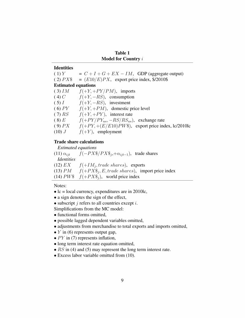
Table 1Model for Country i
Identities( 1) Y = C + I +G+ EX − IM , GDP (aggregate output)( 2) PX$ = (E10/E)PX , export price index, $/2010$Estimated equations( 3) IM f(+Y,+PY/PM), imports( 4) C f(+Y,−RS), consumption( 5) I f(+Y,−RS), investment( 6) PY f(+Y,+PM), domestic price level( 7) RS f(+Y,+PY ), interest rate( 8) E f(+PY/PYus,−RS/RSus), exchange rate( 9) PX f(+PY,+(E/E10)PW$), export price index, lc/2010lc(10) J f(+Y ), employment
Trade share calculationsEstimated equations
(11) αijt f(−PX$/PX$j ,+αijt−1), trade sharesIdentities
(12) EX f(+IMj, trade shares), exports(13) PM f(+PX$j, E, trade shares), import price index(14) PW$ f(+PX$j), world price index
Notes:• lc = local currency, expenditures are in 2010lc,• a sign denotes the sign of the effect,• subscript j refers to all countries except i.Simplifications from the MC model:• functional forms omitted,• possible lagged dependent variables omitted,• adjustments from merchandise to total exports and imports omitted,• Y in (6) represents output gap,• PY in (7) represents inflation,• long term interest rate equation omitted,• RS in (4) and (5) may represent the long term interest rate.• Excess labor variable omitted from (10).
9

depends on output and the domestic price level relative to the import price index.
Consumption and investment depend on output and the interest rate. The domestic
price level depends on output and the import price index. The short term interest
rate depends on output and the price level. It is determined by an estimated interest
rate rule of the country’s monetary authority. The exchange rate depends on the
domestic price level relative to the U.S. price level and on the interest rate relative
to the U.S. interest rate. The export price index depends on the domestic price level
and on an index of world prices. In the estimation the weights on the domestic
price level and the index of world prices are constrained to sum to one. A large
estimated weight on the index of world prices means that the country is primarily
a price taker in the world market. Finally, employment is a function of output.
Note that wages and wealth do not appear in Table 1. It is difficult to get time
series data on these variables. This means that there are no real wage rate and real
wealth effects in the other countries’ models. Other things being equal, a decrease
in PY is expansionary because it leads the monetary authority to lower the interest
rate (RS), which stimulates consumption and investment. However, a potentially
important channel is missing by having no real wage rate and real wealth effects,
and so the the expansionary effects of a decrease in import prices have probably
been underestimated for countries other than the United States.
αijt is the share if i’s exports to j out of the total imports of j in quarter t. It
depends on i’s export price index relative to the export price indices of all the other
countries. The export prices are all in $ per 2010$. The trade share equations are
discussed in the next subsection. The level of exports of country i depends on the
imports of all the other countries and the trade shares. The import price index for
country i, PM , depends on the export price in dollars of each country weighted by
the share of country i’s imports from that country multiplied by E/E10 to convert
to local currency. The index of world prices is the nominal value of the sum of
world exports in dollars divided by the sum of the world exports in 2010 dollars.
The summations exclude the own country and all the oil exporting countries.
10

Trade Share Equations
There is assumed to be one good per country, and the goods are imperfect substi-
tutes. The data are quarterly and are from the Direction of Trade statistics. They
are for merchandise exports and imports. The earliest possible quarter is 1960:1
and the latest is 2016:4. There are 56 countries plus an “all other” category, denoted
AO. The trade share matrix is thus 57×57.
Trade shares have been computed for each pair of countries. As noted above,
aijt denotes the share of i’s merchandise exports to j out of the total merchandise
imports of j in quarter t, where i runs from 1 to 56 and j runs from 1 to 57.
One would expect aijt to depend on country i’s export price relative to an index
of export prices of all the other countries. The empirical work consists of trying
to estimate the effects of relative prices on aijt. A separate equation is estimated
for each i, j pair. The equation is the following:
log(aijt + .00001) = βij1 + βij2 log(aijt−1 + .00001)
+βij3(PX$it/(∑56
k=1 akjt−1PX$kt) + uijt,
t = 1, . . . , T, βij3 < 0.
(1)
PX$it is the price index of country i’s exports, and∑56
k=1 akjt−1PX$kt is an index
of all countries’ export prices, where the weight for a given country k is the previous
quarter’s share of k’s exports to j out of the total imports of j. (In this summation
k = i is skipped.) Equation (1) says that a trade share in quarter t depends on
the trade share in quarter t− 1 and the relative price variable. If the relative price
for quarter t changes from its value in quarter t − 1, the trade share in quarter t
is specified to change from its value in quarter t− 1. This analysis is conditional
on the lagged trade share. No attempt is made to explain why trade shares differ
across pairs of countries. This is the job of trade theory.
With i running from 1 to 56, j running from 1 to 57, and not counting i = j, there
are 3,192 (= 56×57) i, j pairs. There are thus 3,192 potential trade share equations
to estimate. In fact, data limitations prevent all equations from being estimated.
11

Data did not exist for all pairs and all quarters. The estimation periods began
in 1976:1 or later depending on data availability. If fewer than 87 observations
were available for a given pair, the equation was not estimated for that pair. If the
mean of aijt over the sample period were less than 0.005, the equation was not
estimated. Estimated equations were rejected if the estimate of βij2, the coefficient
of the lagged dependent variable, was less than zero or greater than 0.99. Also, if
the estimate of βij3 divided by 1.0 minus the estimate of βij2, which is the estimated
long run effect, was less than -4.0, the equation was rejected. This led to 1,118
pairs being estimated.
The estimation results are summarized in Table 2. The expected sign of βij3 is
negative, and 71.3 percent of the estimates were negative (797 out of 1,118). 31.7
percent of the estimates were negative with a t-statistic in absolute value greater
than 2.0, and 51.3 percent were negative with a t-statistic in absolute value greater
than 1.0. Only 5.5 percent of the estimates were positive with a t-statistic greater
than 2.0, and only 13.4 percent were positive with a t-statistic greater than 1.0.
The results for the quarterly countries only are similar. There is thus support for
equation (1). The average size of the negative estimates of βi3 is -0.286, with a
long run average size of -1.263. In the final specification of the MC model a trade
share equation with the wrong estimated sign was dropped and the trade share was
taken to be exogenous. There are thus 797 estimated trade share equations in the
model. The online appendix to this paper lists the 797 estimated equations.
Finally, in the solution of the model the predicted values of αijt, say, α̂ijt, do
not obey the property that∑56
i=1 α̂ijt = 1. Unless this property is obeyed, the sum
of total world exports will not equal the sum of total world imports. For solution
purposes each α̂ijt was divided by∑56
i=1 α̂ijt, and this adjusted figure was used as
the predicted trade share. In other words, the values predicted by the equations in
(1) were adjusted to satisfy the requirement that the trade shares sum to one.
12
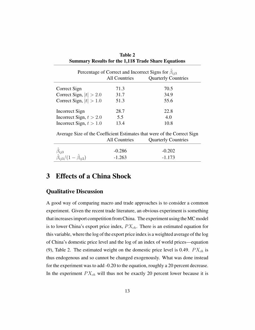
Table 2Summary Results for the 1,118 Trade Share Equations
Percentage of Correct and Incorrect Signs for β̂ij3All Countries Quarterly Countries
Correct Sign 71.3 70.5Correct Sign, |t| > 2.0 31.7 34.9Correct Sign, |t| > 1.0 51.3 55.6
Incorrect Sign 28.7 22.8Incorrect Sign, t > 2.0 5.5 4.0Incorrect Sign, t > 1.0 13.4 10.8
Average Size of the Coefficient Estimates that were of the Correct SignAll Countries Quarterly Countries
β̂ij3 -0.286 -0.202β̂ij3/(1− β̂ij2) -1.263 -1.173
3 Effects of a China Shock
Qualitative Discussion
A good way of comparing macro and trade approaches is to consider a common
experiment. Given the recent trade literature, an obvious experiment is something
that increases import competition from China. The experiment using the MC model
is to lower China’s export price index, PXch. There is an estimated equation for
this variable, where the log of the export price index is a weighted average of the log
of China’s domestic price level and the log of an index of world prices—equation
(9), Table 2. The estimated weight on the domestic price level is 0.49. PXch is
thus endogenous and so cannot be changed exogenously. What was done instead
for the experiment was to add -0.20 to the equation, roughly a 20 percent decrease.
In the experiment PXch will thus not be exactly 20 percent lower because it is
13

affected by the variables in the equation, which are endogenous.
As noted above, each country has an import price index that is a weighted
average of the export prices of the other countries, where the weights are the trade
shares. In the case of the China experiment a country’s import price index will fall
more the larger is the share of China’s exports to the country. And the larger the
fall in the country’s import price index the larger will be the increase in its imports.
In this macro story the increase in imports is driven by the fall in Chinese export
prices. From this perspective the trade literature discussed above starts too late in
the game. ADH, PS, and AADHP begin with with employment changes induced
by increased import competition from China. PS identify increased Chinese com-
petition from PNTR. ADH and AADHP use non-U.S. exposure to Chinese imports
to identify U.S. employment changes due to increased Chinese competition. CDP
use the same identification strategy, but use the implied import changes to back
out productivity increases in China, which are then taken as exogenous for the ex-
periment. Although these experiments do not begin with prices, behind the scenes
it must be that China is able to make inroads into, say, U.S. markets by lowering
the prices of its exports (possibly because of productivity increases).
To return to the MC experiment, if there is no change in the Chinese exchange
rate, then PX$ch decreases the same percent as PXch. This decreases the U.S.
import price index, which from the discussion in the previous section is expan-
sionary. The firm-sector price level falls, as does the nominal wage rate, but the
nominal wage rate falls less and so there is an increase in the real wage rate. This
has a positive effect on household expenditures. Real wealth also increases, which
also has a positive effect on household expenditures. Imports increase because the
relative price of imports decreases, which is contractionary, but as will be seen, the
net effect quantitatively is positive. There may also be positive effects from Fed
behavior via the estimated interest rate rule if the rule calls for a decrease in the
short term interest rate because of the fall in inflation.
14
Consider next the qualitative effects on the rest of the world. It will be useful
to use Table 1 as a guide in discussing the world wide effects of a fall in Chinese
export prices. Consider a decrease in PX$ch. For a given country i the import
price index, PM , falls—(12), which leads to a decrease in the domestic price
index, PY—(6), which leads to a decrease in the export price index, PX—(9).
If PY falls less than PM (which is quantitatively the case), the level of imports,
IM , increases—(5).
Turn now to the trade share equations and calculations. Feeding into the trade
share calculations are larger values of imports and lower values of export prices.
Coming out of the calculations is the level of exports to each country from each
country. In the process each trade share is computed from its estimated equation
(unless the trade share is exogenous). The computed trade share for country i to
country j depends on how much country i’s export price index falls relative to those
of the other countries, weighted by the appropriate lagged trade shares—equation
(1) in the text. The level of exports from i to j depends on the trade share and
the total level of imports of j. Conditional on the trade share, the larger is the
increase in country j’s imports, the large will be country i’s exports. Also coming
out of the trade share calculations is the import price index for each country—
(13). Remember that China is part of these calculations. All was triggered by the
exogenous decrease in China’s export price. In the quantitative results below none
of the decreases in the export prices of the other countries are as large in absolute
value as the decrease in the Chinese export price, and so there is a large relative fall
in China’s export price. China’s trade shares increase, and its exports increase—
(12). This increases output—(1), which leads to an increase in its imports—(3)
and domestic price level—(6).
Coming back to country i, total exports may rise or fall. On the plus side all
countries are importing more, including China. On the minus side if the country
is a large competitor with China (through the trade share calculations), it may lose
out. Also, regardless of China, a country’s export change depends on how large a
15

change there is in the imports of countries that the particular country exports to. The
export change also depends on how much the trade shares change, which depends
on the size of the decrease in country i’s export price relative to the decreases in
the other countries’ export prices.
For countries with estimated interest rate rules, the decrease in inflation leads to
a lower interest rate—(7). This in turns stimulates consumption and investment—
(4) and (5). The net effect on GDP, Y , is ambiguous—(1). It depends on the size of
the increase in imports relative to the size of the increases in exports, consumption,
and investment. If Y does decrease, this will further decrease the interest rate—(7),
which will mitigate the decrease somewhat. Employment, J , moves in the same
direction as Y—(10).
Turn finally to country i’s exchange rate. Whether the country’s currency de-
preciates or appreciates relative to the dollar depends on the change in its domestic
price level relative to that of the United States and on the change in its interest
rate relative to that of the United States—(8). If the currency depreciates (E in-
creases), this will decrease its price of exports in dollars—(2), which feeds into
the trade share calculations. Also, its import price index (in local currency) will
increase—(13). Exchange rate effects can be important because they change a
country’s competitiveness, although exchange rate changes are hard to predict.
The exchange rate equations in the MC model explain very little of the variation
of the exchange rates.
As noted above, missing from the other countries’ models are real wage rate
and real wealth effects. If they were included the China experiment would be more
stimulative than estimated.
16
The Experiment
As noted above, -0.20 was added to the Chinese export price equation. The simu-
lation period is 2000-2007. The estimated residuals were added to the stochastic
equations for this period and taken to be exogenous. This means that when the
model is solved with no changes made there is a perfect tracking solution. The
change is then made to China’s export price equation and the model solved. The
difference between the solution value and the actual value for each variable and
period is the estimate of the effects on the change on that variable for that period.
The results for China and the United States are presented in Table 3. Results are
presented for China for 2002 and 2007, three and eight years after the change
respectively. Results for the United States are presented for 2002:4 and 2007:4,
twelve and 32 quarters after the change respectively.
Effects on China and the United States
The following discussion will focus on results after 8 years or 32 quarters. Consider
China first. Exports are 9.81 percent higher (after 8 years) than in the base case
from the effects of the lower Chinese export prices. This stimulates domestic
demand, and so imports, consumption, and investment are higher. The positive
effects from exports, consumption, and investment outweigh the negative effects
from imports, and so GDP is higher (by 7.27 percent). This stimulus leads to an
increase in Chinese domestic prices: the domestic price level is higher by 11.03
percent. Note that the price of exports is not lower by the full 20 percent of the
shock; it is only down 14.71 percent. It is endogenous and depends on the domestic
price level and the world price index. The former is up and the latter is down, and
the net effect is positive, leading the price of exports not to fall by the full 20
percent. There is no interest rate nor exchange rate equation for China and so no
estimated interest rate nor exchange rate effects. If there were, it is likely that the
Chinese central bank would raise the interest rate (since output and prices are
17

Table 3Summary Results for the
China Experiment
China United States3Y 8Y 12Q 32Q
PM -0.46 -1.33 -2.08 -4.43PY 2.75 11.03 -0.47 -1.61PX -17.30 -14.71 -0.72 -1.98PX$ -17.30 -14.71 -0.72 -1.98PW$ -0.67 -2.10 -2.01 -3.90IM 0.54 4.05 0.65 1.54EX 7.78 9.81 0.08 -0.19C 1.07 4.81 0.31 0.86I 2.43 8.09 0.41 0.72Y 3.00 7.27 0.18 0.42RS 0.00 0.00 -0.04 -0.03E 0.00 0.00 - -
Notes:• See the notation in Table 1.• Values are percent changes from the base
run in percentage points except for RS.• For RS values are absolute changes in
percentage points.• Y = years, Q = quarters.• C for the U.S. is household expenditures
higher), which would likely lead to an appreciation of the yuan. The expansion
would thus not be as large as estimated in Table 3.
Consider now the United States. The price of imports is lower by 4.43 percent,
which leads the domestic price level to be lower by 1.61 percent. This, as discussed
above, stimulates household expenditures through real wage rate and real wealth
effects. Household expenditures are 0.86 percent higher, which has a positive
effect on GDP. The increase in GDP in turn has a positive effect on firm investment
(0.72 percent higher) and imports (1.54 percent higher). The final effect on GDP
18
is that it is 0.42 percent higher. Although not shown in the table, the number of
jobs is 0.44 percent higher, which is an increase of 588,000 jobs. Imports are up
because of the demand stimulus and also because the price of imports fell more
than did the domestic price level. The estimated Fed rule calls for a decrease in the
short term interest rate because of lower prices, but an increase because of higher
output, and the net effect is that the interest rate changed very little: it fell 0.03
percentage points.
U.S. export prices fell due to a fall in the domestic price level and the world
price index. As will be seen, export prices of other countries also fell, and so it
is not clear that a fall in U.S. export prices will lead to a rise in U.S. exports. In
addition, the dollar appreciated relative to other currencies, which has a negative
effect on exports. In fact, U.S. exports were little changed; exports fell by 0.19
percent.
These quantitative results are as expected from the qualitative discussion. The
net effect on U.S. output and employment is positive because of the effects of lower
prices.
Effects on Other Countries
The results for eight other countries (out of 35) are presented in Table 4, seven
quarterly countries and Mexico, which is an annual country. As noted above, there
are no real wage and real wealth effects estimated for other countries, and so any
stimulation from these effects is not accounted for.
For every country the price of imports is lower, due to the effects of the lower
Chinese export prices. Also, for every country except Mexico the domestic price
level is lower. As noted above, the import price index is a significant explanatory
variable in most of the domestic price equations; this is a very robust finding.
Mexico does not have an estimated domestic price equation, which is why it shows
no effect on the domestic price level.
19

Table 4Summary Results for the China Experiment
Canada Japan France Germany12Q 32Q 12Q 32Q 12Q 32Q 12Q 32Q
PM -1.09 -2.39 -3.36 -3.71 -0.81 -1.43 -1.18 -2.10PY -0.19 -1.85 -0.27 -0.74 -0.38 -1.15 -0.15 -1.02PX -0.52 -2.14 -1.13 -2.19 -0.77 -1.47 -0.47 -1.27PX$ -0.62 -2.65 -1.10 -2.43 -0.98 -2.98 -0.68 -2.78PW$ -1.93 -3.75 -1.92 -3.80 -1.92 -3.75 -2.00 -3.82IM 0.50 0.57 0.62 1.28 0.32 0.41 0.38 1.10EX -0.57 -2.30 0.13 0.53 -0.04 0.03 -0.16 -0.16C -0.12 -1.12 -0.02 -0.08 -0.06 -0.03 -0.05 -0.35I -0.11 -1.03 0.00 0.00 0.03 0.36 -0.05 -0.21Y -0.41 -1.78 -0.07 -0.14 -0.11 -0.03 -0.19 -0.69RS -0.09 -0.42 -0.01 -0.03 -0.12 -0.40 -0.12 -0.40E 0.10 0.53 -0.03 0.24 0.21 1.55 0.21 1.55
U.K. Australia Korea Mexico12Q 32Q 12Q 32Q 12Q 32Q 3Y 8Y
PM -1.17 -2.41 -1.88 -3.22 -2.28 -3.08 -1.01 -2.64PY -0.57 -1.87 -0.21 -0.98 -0.11 -0.31 0.00 0.00PX -0.95 -2.18 -0.83 -1.94 -0.93 -1.66 -1.01 -2.13PX$ -1.05 -3.05 -0.93 -2.29 -1.12 -2.51 -1.01 -2.13PW$ -1.90 -3.74 -1.88 -3.73 -1.88 -3.75 -1.76 -3.71IM 0.12 0.11 0.39 0.38 -0.03 -0.11 0.40 -0.16EX -0.04 0.05 -0.41 -0.08 -0.65 0.13 -1.13 -4.66C -0.01 -0.01 -0.11 -0.27 -0.07 -0.06 -0.39 -2.29I -0.01 -0.02 -0.10 -0.20 -0.01 -0.03 0.00 0.00Y -0.05 -0.03 -0.22 -0.30 -0.24 0.07 -0.65 -2.81RS -0.09 -0.12 -0.19 -0.38 0.00 0.00 0.00 0.00E 0.10 0.90 0.09 0.35 0.20 0.88 0.00 0.00
See notes to Table 3
20

For every country except Korea and Mexico imports rise, which is because
import prices fell more than did the domestic price level. The relative price variable
is not in the Korea import equation, which is why Korean imports did not rise. More
will be said about Mexico later. For every country the price of exports in dollars
fell, due to the fall in the domestic price level and world export prices. Whether
exports increase or decrease in this case depends on the fall in a country’s export
price index relative to other countries’ indices and on the trade share calculations.
Exports rose slightly for Japan, France, the United Kingdom, and Korea and fell
for the others.
The net effect on total output is positive for Korea and negative for the others.
The monetary authorities responded to lower prices and lower output by lowering
the short term interest rate (except for Korea and Mexico, which do not have an
estimated interest rate equation). The lower interest rates have positive effects
on consumption and investment. The decreases in the interest rates were larger
than the decrease in the U.S. rate, and this led to a depreciation of the countries’
currencies relative to the dollar (E is higher). The prices of exports in dollars thus
fell more than the prices of exports in local currency. This has a positive effect on
exports.
There was a fairly large fall in Canada’s exports (-2.30 percent), which led to
a fairly large fall in total output (-1.78 percent). The same is true for Mexico. For
all countries the fall in the price of exports was much smaller than the fall in the
price of exports of China, and so all countries lost market share to China. Canada
and Mexico are large exporters to the United States, and the trade share estimate
and calculations are such that there are large decreases of Canadian and Mexican
exports to the United States. These two countries are the most effected of all the
countries by the China shock. This result depends, other things being equal, on
the trade share coefficient estimates, and in this sense they are empirically based.
The main point about the results for the other countries is that output is generally
slightly lower because of the loss of exports to China. The declines are smaller than
21

otherwise because of lower interest rates and depreciated currencies and because
world demand is stimulated by increases in most countries’ imports. Again, this
is absent real wage rate and real wealth effects, which would be stimulative.
4 Comparison with Trade Models
I began this study thinking I could compare the experimental results from the MC
model just described to those from a model like the CDP model, but the model
building methodologies are not similar enough for this to be sensible. Following
the CC approach, the MC model is a standard textbook simultaneous equations
models, nonlinear. It can be easily solved numerically using Gauss-Seidel. The
coefficient estimates are based on data as far back as 1954.
The CDP model is a model of 22 sectors, 37 countries not counting the United
States, and 50 U.S. states. For a given sector there is potential trade between
each pair. Also, for a given sector there is potential labor migration between each
pair of U.S. states. Trade elasticities are estimated. If trade elasticities differed
across sectors and pairs, there would be 22 × 88 × 87 = 168, 432 parameters to
estimate. If fact, estimates are obtained for only 12 sectors, so the potential number
of parameters is 91,872. If these parameters were constant across time, they could
in principle be estimated with enough data over time. The assumption is made,
however, that for a given sector all the parameters are the same, so there are only
12 parameters to estimate. These are estimated using cross section data for 1993.
The theoretical specification of the model is tight, based on the assumption of
perfect foresight, and it is constructed to have a steady state. The structure is such
that the model cannot be solved in closed form without the assumption of equal
sector elasticities across pairs. A similar story concerns migration elasticities.
There are potentially 29,400, but they are all assumed to be the same, so only one
parameter is estimated. In this case it is estimated using data across time. Again,
this assumption is required to be able to solve the model in closed form. There is
22
one calibrated parameter in the model, the discount rate, set at 0.99 per quarter.
The China experiment that CDP run is similar to the one in this paper in that
there is increased Chinese import competition. For comparison purposes, it is
informative to consider how, say, exports from Germany to France are affected
in the experiment. For the MC model there are five estimated equations that
are important for this determination: the domestic price equation for Germany—
(6) in Table 1, the import equation for France—(3), the export price equation for
Germany—(9), the Euro exchange rate equation—(8), and the trade share equation
forαGE,FR. The first equation is estimated for the 1961:1-2017:2 period, the second
for 1961:1-2017:4, the third for 1965:1-2016:4, the fourth for 1972:2-2017:4, and
the trade share equation for 1976:1-2016:4. In the solution after the shock (where,
of course, the entire MC model is involved), the effects on the first four variables
are listed in Table 4. For reasons discussed in the previous section, Germany’s price
of exports in dollars falls (by 2.78 percent after 32 quarters). For the trade share
calculations this price needs to be compared to∑56
k=1 akjt−1PX$kt in equation (1) in
the text, where j is France and the summation skips Germany. Although not shown
in the table, this variable decreased more than did PX$GE (driven by the large fall
in the Chinese export price), and so the ratio in equation (1) increased, which has a
negative effect on the trade share αGE,FR. On the other hand, French total imports
rose, and the net effect on exports from Germany to France was positive: the level
of exports rose 0.41 percent, which is $123 million. This result could clearly go
either way; the sign depends on the sizes of the coefficient estimates in the various
equations. Regarding exports from France to Germany, it turns out that these are
down 0.51 percent after 32 quarters—$104 million.
For the CDP model the exports from Germany to France are based on the 12
estimated elasticities, estimated using 1993 data. The level of detail is much larger
since there are 12 tradeable sectors compared to one good per country for the MC
model. On the other hand, there are many more coefficients estimates in the MC
model—about 1,000 in the estimated structural equations and 797 × 3 = 2, 391
23
in the estimated trade share equations—based on data back as early as 1954. The
empirical strategies are thus vastly different. In this case, unlike in the DSGE case,
the difficultly of making comparisons is not because the CDP model is calibrated,
which is isn’t except fot the discount factor. It’s that so much is based on so few
estimated coefficients.
5 Conclusion
Focusing on the United States, a fall in Chinese export prices is stimulative in
the MC model. Domestic prices fall, real wage rates and real wealth rise, and
household expenditures increase. It may also be that the Fed lowers the interest
rate due to lower prices, which is stimulative, although this is ambiguous since
higher output has a positive effect on the interest rate through the estimated Fed
rule. It may also be that the dollar appreciates, which has a negative effect on
output. But the net effect in the model is positive. These channels are missing
from most trade models, and so in the case of the China experiment the models
have likely overestimated the negative or underestimated the positive employment
effects of increased Chinese import competition.
Note that this is an aggregate result. It may be that some sectors and regions in
a country or state are adversely affected by increased Chinese import competitions,
where output and employment are down. Behind the aggregate result is the situation
that other sectors and regions (and even possibly individuals within the negatively
affected sectors and regions) are helped by the increased aggregate demand caused
by the lower prices.
Finally, from the perspective of the Cowles Commission approach, trade mod-
els are far removed from the data. The level of disaggregation can be very large,
but few parameters are estimated relative to the size of the models. Also, the dy-
namics don’t seem likely to be well captured. A question like the effects on the
economy from increased Chinese import competition is a dynamic question, but
24

time series data are used sparingly in trade models. Many of the paramter estimates
are typically based on one cross section of data. Dynamic results from many trade
models thus have little empirical support, in addition to not taking into account
macro effects.
25

References[1] Acemoglu, Daron, David Autor, David Dorn, Gorden H. Hanson, and Bren-
dan Price, 2016, “Import Competition and the Great US Employment Sagof the 2000s,” Journal of Labor Economics, 34, S141–S198.
[2] Autor, David H., David Dorn, and Gordon H. Hanson, 2013, “The ChinaSyndrome: Local Labor Market Effects of Import Competition in the UnitedStates,” American Economic Review, 103, 2121–2168.
[3] Caliendo, Lorenzo, Maximiliano Dvorkin, and Fernando Parro, 2019,“Trade and Labor Market Dynamics: General Equilibrium Analysis of theChina Trade Shock,” Econometrica, 87, 741–835.
[4] Fair, Ray C., 2018, Macroeconometric Modeling: 2018,fairmodel.econ.yale.edu/mmm2/mm2018.pdf.
[5] Fair, Ray C., 2019, “Some Important Macro Points,” July, forthcomingOxford Review of Economic Policy.
[6] Pierce, Justin R., and Peter K. Schott, 2016, “The Surprisingly Swift De-cline of US Manufacturing Employment,” American Economic Review, 106,1632–1662.
26
Top Related