


Languages
Pages
Legal


Trade Liberalization, Antidumping, and Safeguards:
Evidence from India's Tariff Reform
Chad P. Bown†
Brandeis University Patricia Tovar‡
Brandeis University
This version: May 2009
Abstract
This paper is the first to examine empirically the relationship between import tariff cuts and the subsequent re-imposition of import protection under safeguard exceptions at the product-level. Our approach overcomes potential endogeneity problems by focusing on the case of India, a country that underwent a major exogenous tariff reform program in the early 1990s and subsequently initiated substantial use of safeguard and antidumping import restrictions. In the first part of the paper we estimate structural determinants of India’s import protection using the Grossman and Helpman (1994) model. Estimates of the model on India’s pre-reform tariff data from 1990 are consistent with the theory. We then re-estimate the model on the Indian tariff data after the trade liberalization is complete and find that the model no longer fits, a result consistent with theory and evidence provided in other settings that India’s 1991-92 IMF arrangement can be interpreted as resulting in an exogenous shock to India’s tariff policy. However, when we re-estimate the model on data from 2000-2002 that more completely reflects India’s cross-product variation in import protection by including both its post-reform tariffs and its additional non-tariff barriers of antidumping and safeguard import protection, the significance of the Grossman and Helpman model determinant estimates is restored. In the paper’s second section we use a reduced form model to pursue additional questions regarding India’s late 1990s and early 2000s new use of antidumping and safeguard protection. While we confirm the result that products with larger tariff cuts between 1990 and 1997 are associated with a substitution toward these new forms of import protection in the early 2000s, the estimates are also economically important and provide one explanation for separate results in the literature that the magnitude of import reduction associated with India's use of antidumping is similar to the initial import expansion associated with its tariff reform. Finally, we interpret the implications of our results for the burgeoning research literature examining the effects of liberalization on India’s micro-level development.
JEL No. F13 Keywords: India, tariff reform, antidumping, safeguards, political economy ________________
† Bown: Department of Economics and International Business School, MS021, Brandeis University, Waltham, MA 02454-9110, USA tel: 781-736-4823, fax: 781-736-2269, email: [email protected], web: http://www.brandeis.edu/~cbown/. ‡ Tovar: Department of Economics and International Business School, MS021, Brandeis University, Waltham, MA 02454-9110, USA tel: 781-736-5205, fax: 781-736-2269, email: [email protected], web: http://www.brandeis.edu/~tovar/ . Thanks to Robert Staiger, Nuno Limão, Meredith Crowley, Steve Redding, Bernard Hoekman, Marcelo Olarreaga, T.N. Srinivasan, Hylke Vandenbussche, Jaimie de Melo, Giovanni Facchini, Sajal Lahiri, Kamal Saggi, Maurizio Zanardi and seminar participants at LSE, Seoul National University, the University of Geneva, and the MWIEG meetings in Michigan for helpful comments. Olivier Cadot, Jean-Marie Grether, and Marcelo Olarreaga also shared useful data. Bown acknowledges financial support from the World Bank and thanks the WTO for hospitality while a portion of this paper was being written. All remaining errors are our own, and any opinions expressed within are our own and should not be attributed to the World Bank or the WTO.

1 Introduction
India undertook a substantial episode of unilateral trade liberalization beginning in 1991-1992, one in
which it dramatically cut its import tariffs in a process that continued until 1997. Its import-weighted
average tariff declined from 87.0 percent in 1990-1991 to 24.6 percent in 1996-1997. Before 1992, India
had never resorted to using the “safeguard” exceptions embodied in many trade agreements, such as
antidumping or a global safeguard, to implement import restrictions that are common alternatives to
tariffs. By the period 1997-2002, however, India had transformed from a non-user to become the WTO
system’s most prolific user of these alternative, non-tariff barriers to trade. In the case of antidumping, the
vast majority of Indian investigations resulted in the imposition of new import restrictions, and most of
them remained in effect for five years or more. As figure 1 indicates, by 2002, India had enough new
antidumping trade barriers in place to cover 132 different 6-digit Harmonized System tariff lines.
Combined, the potential exogeneity of India’s import tariff cut and the fact that it had no history
of using antidumping or safeguard trade restrictions before the liberalization episode make the Indian
experience a relatively unique testing environment in which to examine whether there is a relationship
between tariff liberalization and the subsequent imposition of these non-tariff barriers to trade. This paper
introduces a new approach to empirically investigate a potential link between trade liberalization and the
subsequent use of such trade agreement “exceptions” that permit these forms of new import protection.
Our setting of the “natural experiment” created by India’s exogenously-mandated tariff reform
program of the 1990s allows us to overcome many potential endogeneity concerns associated with
examination of the relationship between trade liberalization and the resort to new protection under
safeguard exceptions. The first endogeneity concern is that a country's trade liberalization is typically not
itself an exogenous event, but instead is part of a negotiated preferential or multilateral trade agreement.
In such cases, endogenous factors may determine both the level of initial liberalization and subsequent
resort to exceptions for new protection. Focusing on a single country like India with an exogenous tariff
cut allows examination of the effect of the tariff cut treatment on subsequent response of new import
protection. A second endogeneity concern may arise if the trade liberalizing country is simultaneously
1
negotiating the terms of the “exceptions” in the writing of the trade agreement – i.e., not only the question
of whether to have any exceptions at all, but also the legal and economic evidentiary criterion that must
be met in order to trigger the exceptions. This is also not of concern for our context as India’s accession to
the WTO was part of the “Single Undertaking,” which meant India would be subject to established
GATT/WTO rules governing antidumping and safeguard exceptions.
Our approach is to use the Indian setting and exploit cross-product variation to examine whether
there is a link between size of the initial tariff cut and the subsequent resort to such new import
restrictions. In particular, we focus on the product-level link between India’s tariff cuts and its later resort
to the liberal trade policy “exceptions” of newly applied global safeguard and antidumping trade
restrictions, which themselves are relatively substitutable forms of import protection.1
In addition to the exogeneity of its tariff reform, India is an excellent setting to test for this link
for a number of reasons that we detail further in section 2. Following the initiation of its tariff reform
program in 1991, India transformed from being a non-user of policy exceptions such as antidumping and
safeguards to becoming the WTO system’s most frequent user (WTO, 2009a,b) of both types of import
restrictions over the next decade. Nevertheless, while the response to the Indian tariff reform program
appears well timed with the subsequent rise in filings and implementation of these safeguards and
antidumping policy exceptions, is there a product-level link? Figure 2 illustrates suggestive evidence of
the basic relationship between the relative sizes of the 1990s tariff cuts and subsequent antidumping use.
The figure indicates that products that sought and were granted antidumping protection in effect by 2002,
on average started with higher tariffs and received larger tariff cuts between 1990 and 1997. Our
econometric analysis investigates whether this suggestive evidence of a relationship between the size of
1 Despite substantial legal differences between safeguards and antidumping, they have been shown in many contexts to be relatively substitutable instruments of import protection, given the lax enforcement rules regulating how these policies are implemented. See, for example, Bown (2004), Bown and McCulloch (2003) and also the discussion in Hoekman and Kostecki (2001). Nevertheless, our estimation approaches control for the most important differences (e.g., antidumping is country-specific and discriminatory, safeguards are nondiscriminatory) between them as we describe in substantial detail below. For comprehensive surveys of economic research in the antidumping literature see Blonigen and Prusa (2003) and for the safeguard literature, see Bown and Crowley (2005).
2

the trade liberalization and subsequent resort to these policy exceptions is economically and statistically
important. The formal approach that we adopt is two-pronged.
In section 3 we present our first econometric approach by adopting the Grossman and Helpman
(1994) model to estimate structural determinants of India’s import protection. We first estimate the model
on India’s pre-reform tariff data from 1990 and present results that are broadly consistent with the theory
and evidence from other countries and trade policy settings. 2 To examine the potential exogeneity of
India’s tariff cut, as a second step we re-estimate the Grossman and Helpman model on the Indian tariff
data from years after the trade liberalization is complete. The results suggest that the model no longer fits
the data, a result consistent with theory and evidence provided in other settings that India’s 1991-92 IMF
arrangement can be interpreted as resulting in an exogenous shock to India’s tariff policy. In particular,
we find that the trade liberalization resulted in cross-product variation in the new level of Indian import
tariffs that can no longer be explained by political-economic determinants of the model. As a third step,
we then re-estimate the Grossman and Helpman model on data from 2000-2002 that more completely
reflects India’s cross-product variation in import protection. When we measure India’s 2000-2002
protection by including both its post-reform tariffs and its additional non-tariff barriers of antidumping
and safeguard import protection, the evidence indicates a restoration of the significant determinants of the
Grossman and Helpman model. Furthermore, the relationship is driven by product-level variation within
relatively important Indian industries such as iron, steel and fabricated metal products, chemicals, food
products, and transport equipment, which include industries that are both major Indian users of
antidumping and sectors with a large share of India’s manufacturing imports.
2 The first papers to estimate structural versions of the Grossman and Helpman model on data for the United States include Goldberg and Maggi (1999) and Gawande and Bandyopadhyay (2000). While there are too many studies in the subsequent literature to cite here, Cadot, Dutoit, Grether and Olarreaga (2008) is the first paper that we are aware of that applies the Grossman and Helpman model to determinants of Indian import protection. Nevertheless their study does not examine the questions of interest of this paper - i.e., specifically whether the model can be used to understand determinants of a particular trade policy (antidumping and/or safeguards) as well as whether there is a relationship between demands for such forms of protection and the size of past trade liberalization.
3

In section 4, the second prong of our approach is to adopt a reduced form model to pursue
additional questions regarding India’s late 1990s and early 2000s use of antidumping and safeguard
protection. First, from this setting we provide confirming evidence of a significant negative relationship
between the size of the product-level trade liberalization undertaken between 1990 and 1997 and the
subsequent resort to new protection in the early 2000s – i.e., the larger the good's initial tariff cut, the
more antidumping and safeguards protection the Indian producers of that good demanded and received ex
post. 3 We also find that India's imports of products from countries that have recently targeted Indian
exporters in the same 4-digit industry with antidumping are in turn less likely to be the target of Indian
antidumping, which could be due to a fear of future retaliation. 4 Finally, products with a smaller “tariff
overhang” (i.e., the difference between the WTO tariff binding and India’s applied tariff rate) are more
likely to use antidumping, as we would expect.
We also document in section 4 the economic significance of the estimates and their implications
for other areas of the research literature. We find that the average effect is large – i.e., a one standard
deviation increase in the tariff cut away from the mean increases the predicted probability of new
antidumping use by about 30%, and of new antidumping or safeguard use by 24%. We present additional
evidence in which we investigate a previously unexamined margin of the data on the duration of time that
measures stay imposed. Within the set of Indian products receiving antidumping protection, there is also a
negative relationship between the length of protection under an antidumping measure and the size of the
3There are some papers related to our approach but which use much more aggregated data and which also do not attempt to deal with the endogeneity issues that we have identified. For example, Crowley (2009) is a cross-country, macro-level study relating the subsequent number of safeguard cases that a WTO member initiated between 1995 and 2000 to a measure of the member's average tariff cut undertaken in the Uruguay Round. Feinberg and Reynolds (2007) is a similar cross-country approach which focuses on antidumping alone and is carried out at a very aggregated industry level. Our approach differs from these two studies along a number of dimensions, including that it focuses on a single country in which the tariff cuts were arguably exogenous thus forming the basis for a better natural experiment, it is conducted at the product (6-digit Harmonized System) level, it examines both antidumping and safeguard use, and the estimates derive not only from reduced-form but also structural econometric models. 4 See Prusa (1992) and Hoekman and Mavroidis (1996), for example, for discussions. Recent papers finding evidence consistent with retaliatory effects on different samples of antidumping use data include Blonigen and Bown (2003), Prusa and Skeath (2002), Feinberg and Reynolds (2006) and Vandenbussche and Zanardi (2008). Note that none of these earlier empirical papers match antidumping use across countries at the actual level of product disaggregation (6-digit Harmonized System) that we have done here.
4

1990s tariff cut. We thus find that "temporary" antidumping protection may be more likely to become
"quasi-permanent" protection the larger was the product's original tariff cut. We summarize the
implications of these results in section 4.8. In particular, our estimates provide one explanation for
separate results in the literature that the magnitude of import reduction associated with India's use of
antidumping is similar to the initial import expansion associated with its tariff reform. 5 Furthermore, we
are also able to interpret the implications of our results for the burgeoning research literature examining
the effects of the 1990s trade liberalization on patterns to India’s micro-level development.
Before turning to the next section, we also take care to identify the limits to the implications of
our results vis-à-vis other important questions raised by the theoretical literature on trade agreements and
“safeguard” type-exceptions. For example, economic theorists have identified how a trade agreement that
grants exceptions that allow for a government to re-implement conditional import protection after trade
liberalization occurs can help facilitate trade liberalization ex ante.6 Since we only focus on India’s
import protectionist response (via use of antidumping and safeguards) to its exogenous trade liberalization
episode, our results can not speak to the important broader question of whether ex post access to these
exceptions facilitates a country’s willingness to liberalize its import tariffs in the first place.
2 India’s Tariff Reform, Antidumping, and Safeguards
2.1 Trade liberalization in India in the 1990s
Between 1947 and the late 1980s, India followed an inward-oriented development strategy. A
combination of external shocks in the late 1980s and early 1990s led to large macroeconomic imbalances,
5 The size of our estimates for India that link trade policies (tariffs and antidumping/safeguards) over time indicate economically important implication for trade flows and provide evidence consistent with Vandenbussche and Zanardi (2006), whose gravity model estimates find that the trade decrease resulting from India’s antidumping policy is of the same magnitude as the trade increase that resulted from its earlier trade liberalization. 6 For example, Bagwell and Staiger (1990) illustrate how safeguards can play a positive role in maintaining a cooperative trade agreement and relatively low tariffs in the face of unexpected shocks. A separate strand of the theoretical literature on trade agreements (e.g., Staiger and Tabellini, 1987; Maggi and Rodriguez-Clare 1998, 2007) finds that ex ante inclusion of such a safeguard exception can create time-consistency or commitment problems that make it difficult for a government to implement even Pareto-improving trade liberalizing reform announcements ex post. Our approach does not specifically address this literature either.
5
and as a result, India requested a stand-by arrangement from the International Monetary Fund in August
of 1991. Among the conditions for the arrangement was that India had to implement major structural
reforms, including trade liberalization, financial sector reform and tax reform (Cerra and Saxena, 2002).
The trade reform started in 1991 and was completed within the export-import policy announced
in the government’s Eighth Plan in 1992, which outlined a program of tariff reductions for the next five
years on the basis of the 1991 agreement with the IMF (Pursell, Kishor, and Gupta, 2007). 7 The
government had to meet strict compliance deadlines, and it chose to implement the reform abruptly so as
to avoid the emergence of potential opposition and thus without time to analyze or debate its distributive
effects (Topalova, 2006). Such tariff reform characteristics point to its exogenous nature.
As additional evidence on the exogeneity of the tariff reductions, Edmonds, Pavcnik and
Topalova (2007) report a marked linear relationship between the pre-reform tariff levels and the tariff cuts
by industry – which we also confirm using our data – deriving from the fact that the IMF mandated a
reduction in both the tariff levels and their dispersion. Moreover, Topalova (2005) regresses the tariff
change on late 1980s industry characteristics, including factor shares, concentration, employment, wages,
productivity and others, and finds that tariff changes are not correlated with industry characteristics.
Prior to the IMF arrangement, the 1990-1991 Indian import-weighted average tariff was 87
percent, the simple average was 128 percent, and some tariffs were over 300 percent (Srinivasan, 2001).
The maximum tariff fell from 355 percent in 1990-1991 to 150 percent in 1991-1992 and 30.8 percent in
2002-2003. The weighted average tariff decreased from 87 percent in 1990-1991 to 24.6 percent in 1996-
1997 before it gradually increased to 38.5 percent in 2001-2002.8 Finally, the standard deviation of tariffs
fell from 41 percent to 15 percent between 1991 and 1997-1998 (Hasan, Mitra, and Ramaswamy, 2007).
7 Even though India was a member of the GATT, it did not participate in tariff-reducing GATT rounds (Edmonds, Pavcnik and Topalova, 2006). Topalova (2004) also describes these five-year plans as having been carried out largely as they were originally announced. 8 The increase in applied tariffs after 1997 coincided with a significant lifting of quantitative restrictions (Narayanan, 2006) and was possible because India’s tariff bindings from the Uruguay Round were set at much higher levels than the applied rates (Srinivasan, 2001). The simple average tariff rate fell from 128 percent in 1990-1991 to 34.4 percent in 1997-1998 and then increased to 40.2 percent in 1998-99 but continued decreasing after that (Narayanan, 2006).
6

Because of the exogenous nature of India's IMF-mandated trade liberalization in the 1990s, a
number of researchers have used it as a "natural experiment" case study to test the impact of trade
liberalization on many different questions concerning fundamental microeconomic activity.9 However,
one concern that we examine is the extent to which this exogenous reduction in import tariffs is positively
associated with the subsequent re-application of new forms of import protection in India via WTO-
permitted exceptions such as the imposition of safeguards and antidumping import restrictions.
2.2 India's antidumping and safeguard policies and use
Table 1 documents how the pattern of new Indian antidumping initiations evolved over the 1992-2004
period. India introduced its antidumping legislation in 1985 but did not initiate its first antidumping case
until 1992 and after its tariff reforms had begun. Furthermore, India enacted its domestic safeguard
legislation in 1997 and did not initiate its first safeguard investigation until that year. The use of
antidumping in particular accelerated in the late 1990s before reaching its peak in 2002.10 As table 1
illustrates, India initiated 380 antidumping cases during that period. India imposed a final antidumping
measure - e.g., typically an ad valorem or specific duty - in 295 of the investigations, representing 85
percent of the number of initiations with non-missing data on final decisions (348).11 Thus not only did
India initiate a large number of cases, but a very large majority of these cases resulted in the imposition of
new trade restrictions. India imposed final measures in 8 of the 12 safeguard cases with non-missing data
9 We further discuss and assess the potential implications of our results for this literature below in section 4.8. 10 Our analysis draws on the publicly available Global Antidumping Database (Bown, 2007) which provides detailed data on policy investigation outcomes, as well as products and exporting countries targeted by Indian use of antidumping between 1992 to 2004. The working paper accompanying the database describes the data in full detail. To summarize, the data for India was taken directly from what the Directorate General of Antidumping and Allied Duties in the Ministry of Commerce publicly reported in The Gazette of India http://commerce.nic.in/ad_cases.htm. The information on the duration of measures imposed was frequently supplemented by information India has made available to the WTO's Committee on Antidumping. 11 While we do not report it in the table, in 26 cases no evidence of dumping was found and in 33 cases no injury was found. Only 10 cases were withdrawn or terminated. Furthermore, in 289 of the 314 observations with non-missing information (92 percent), a preliminary duty was imposed implying that in almost all cases, petitioning firms received at least temporary protection from imports.
7

during this time period. Finally, India's use of both antidumping and safeguards went unchallenged by
WTO members through formal Dispute Settlement Understanding activity until December 2003, when
the European Union brought the first case against Indian antidumping (WTO, 2008). 12
Table 2 decomposes the Indian use of antidumping and safeguards over the 1992-2004 period for
industries within the manufacturing sector. The dominant user of antidumping and safeguards is industrial
chemicals, with 214 antidumping initiations and nine safeguard initiations. Other frequent users of
antidumping are iron and steel (36), other chemicals (18), machinery except electrical (17) and machinery
electric (14). Among industries that initiated safeguard investigations, each was also a user of India's
antidumping policy during this time period.
2.3 The economic importance of Indian antidumping and safeguard industry-level users
Are the industry-level users of these Indian policies economically important? Table 2 also presents
information on the relative size of imports across sectors. Over the period 1992-2004, industrial chemicals
was not only the most frequent user of antidumping and safeguards within India, it also competed with
the largest value of imports among all Indian manufacturing industries, representing 15 percent of all
Indian manufacturing imports (and 16 percent in 1988-2004). In some years industrial chemicals
represented almost 20 percent of manufacturing imports, despite the potential trade destructive effects of
the imposition of new Indian antidumping and safeguard import restrictions. The other major industrial
users of antidumping and safeguards also face substantial competition from imports. An implication is
that use of these policies has potentially distorted incentives and activities in significant areas of the
Indian economy.
12 A contributing explanation to the high incidence of Indian industry "success" in antidumping and safeguard investigations (i.e., such a high share resulting in the imposition of final measures) is thus that India's use of antidumping and safeguards was not formally challenged by any trading partners under the WTO's dispute settlement provisions until December 2003. Nevertheless, Indian exporters during this time period were increasingly targeted by other WTO members’ use of antidumping, as the WTO (2009) reports that its members initiated 107 antidumping cases against India between 1995 and 2004 alone. India as a target of foreign antidumping was only surpassed by cases against China, Korea, the U.S., the EC and its member states, Taiwan, and Japan during this time period, despite India having a much smaller level of exports than these other countries.
8

Finally, when we match antidumping use and trade data at the 6-digit Harmonized System (HS)
level, we find that 14 percent of Indian manufacturing imports in 1991 were in products that would
subsequently become affected by antidumping or safeguards between 1992 and 2004. When we consider
the average of imports from 1992-2004, 12 percent of Indian manufacturing imports between 1992-2004
were in products affected by antidumping or safeguard initiations.13 While this serves as a potential upper
bound on the impact of India's use of antidumping on trade flows during this time period, it reinforces the
importance of a more in depth examination of India’s use of antidumping and safeguards.14
3 The Grossman and Helpman Econometric Approach and Results
3.1 Econometric model
Our first econometric approach builds on the Grossman and Helpman (1994) model of trade protection.
Their approach has become the leading political economy model of trade protection as it begins from first
principles and derives a set of testable predictions about the determinants of protection based on
government-industry interaction. The model assumes a small open economy in which there is a numeraire
good produced only with labor, and i = 1, …, n non-numeraire goods produced with labor and a specific
factor. The specific factor owners may organize into lobby groups and simultaneously offer the
government a contribution schedule that maps each government policy choice into a campaign
contribution level. In the second stage, the government selects the trade policy vector to maximize a
weighted sum of contributions and social welfare. The model provides the following equation for
equilibrium tariffs:
13 When measured as a share of all Indian imports, these figures are 9 percent and 7 percent, respectively. In the same period, the share of tariff lines in manufactures for which there was an antidumping or safeguard initiation is 5 percent and the share of all tariff lines is 4 percent. Table 2 also shows the share of HS-6 tariff lines for which there was an AD initiation within each 3-digit ISIC sector, as well as the share of imports that those HS-6 products represent. 14 This is an upper bound because antidumping investigations and measures are typically applied at the 8-digit level, and not all 8-digit products within a 6-digit HS category will necessarily be targeted.
9

i
i
L
Lii
zaIt
εαα
⋅+−
= , (1)
where is the ad valorem tariff; is an indicator variable that equals one if the sector is organized into
a lobby and zero otherwise;
it iI
Lα denotes the fraction of the population that owns some specific factor; a is
the weight that the government places on social welfare relative to political contributions; is the
equilibrium ratio of domestic output to imports; and
iz
iε is a measure of the absolute value of the elasticity
of import demand defined as follows: ( ))()( *iiiiii pmppm′−=ε , where in turn denotes imports of good
i, and and denote the domestic and world price of good i, respectively.
im
ip *ip 15
Our strategy is to proceed as follows. We begin by testing the Grossman and Helpman model’s
equation (1) for India’s applied tariffs in 1990. This is the year prior to India's trade policy reform and
thus the last year its tariffs were determined endogenously. The objective is to verify whether the
Grossman and Helpman model is an appropriate predictor of India’s trade policy in the absence of an
exogenous mandate of reform. If we find support for this hypothesis, the next step is to estimate equation
(1) for India’s applied tariffs after the reform and thus in the period 2000-2002.
Since subsequent to the August 1991 IMF agreement Indian tariffs were affected by an
exogenous mandate, we would expect to find that the Grossman and Helpman model does not adequately
predict India’s applied tariffs by themselves in 2000-2002. However, as table 1 and figure 1 indicate,
India had become a relatively heavy user of antidumping by the early 2000s. If India were exogenously
constrained so that it cannot increase its applied tariffs, as arguably took place when India committed to
reduce its tariffs under the agreement with the IMF, antidumping or safeguard duties could be used as a
substitute policy instrument. Therefore, we then estimate the Grossman and Helpman model for tariffs
plus antidumping and safeguard duties in 2000-2002 as the dependent variable.
15 To obtain iε from the elasticity defined over domestic prices, , that we use in the estimation, we would need to
divide the latter by ie
)1(*iii tpp += . However, since output is measured at domestic prices while imports are
measured at world prices, we also need to divide by iz )1( it+ , which is equivalent to saying that we can directly use instead of ie iε in equation (1) in the estimation.
10

If we find support for the Grossman and Helpman model once antidumping and safeguard duties
are included in the protection measure, we interpret the combined results (i.e., support for the Grossman
and Helpman model for tariffs in 1990; lack of support for the model for tariffs in 2000-2002; and support
for it for tariffs plus antidumping and safeguards in 2000-2002) as evidence that, while the trade
liberalization reform moved tariffs away from the Grossman and Helpman equilibrium, the use of
antidumping and safeguards generated a movement back toward the protection levels that would be
predicted by that model. In other words, this would provide evidence that antidumping and safeguards
were used as a substitute for tariffs.
Based on (1), we define the estimation equation as follows:
titi
i
ti
iiti
zzI ,210, μ
εβ
εββτ +⎟⎟
⎠
⎞⎜⎜⎝
⎛+⎟⎟
⎠
⎞⎜⎜⎝
⎛×+= , (2)
where the dependent variable may defined as the applied tariff only or also include AD/SG duties, t
equals either 1990 or 2000-2002, 0)(11 >+= La αβ , 0)(2 <+−= LL a ααβ and iμ is the regression
error term. 16 Protection increases with ( )iiz ε for organized sectors and decreases in the case of
unorganized sectors. The magnitude of the deviation from free trade (in either direction) is thus higher
when ( iiz )ε is higher, because a larger output means the benefit from protection is higher for the lobby,
and the welfare cost from protection is lower the lower are the volume of imports and the elasticity of
import demand. The Grossman and Helpman model also predicts that 021 >+ ββ . Finally, from 1β and
2β we can retrieve the estimated values of the model parameters a and Lα , defined above.
16 The error term is included to capture potential measurement error in the variables and other factors (not accounted for in the model) that may influence the determination of trade policy.
11

3.2 Data
3.2.1 Tariffs, antidumping and safeguard policies
First we estimate the model for data from the pre-reform year of 1990. Tariff reductions in India took
place mostly between 1991 and 1997, and India began to increase its use and application of safeguards
and antidumping in 1997 (table 1 and figure 1). As the data on output is available only until 2001, we
perform the estimation for our second set of results on averages over 2000-2002 (where for 2002 we use
data on output in 2001). Depending on the specification, for these estimates we use as the dependent
variable the average of applied tariffs from 2000-2002 or the combination of the average applied tariffs
plus the antidumping or safeguard (AD/SG) protection in force during 2000-2002.17
We estimate the Grossman and Helpman model on a cross-section of data, and our unit of
observation is an imported product at the 6-digit Harmonized System (HS) level either in 1990 or
averaged over 2000-2002. The Indian applied ad valorem tariff data for 1990 and for 2000-2002 at the 6-
digit HS level is obtained from the WTO’s Integrated Database available in WITS.
For our last set of specifications we use the sum of the applied tariff and an AD ad valorem
equivalent. This variable was constructed using data at the exporter-product level and requires some
discussion. While most Indian AD measures were imposed as specific duties, we also have data on the
final margin calculation in ad valorem terms.18 In some cases this is reported as a range for each firm,
from a minimum to a maximum value. Therefore, for each AD case we calculate two variables: i)
AD_min, which is the average of the minimum AD margin over all firms in the foreign country that is
being subject to an Indian AD measure; and ii) AD_max, defined analogously as the average of the
17Tariff data is available for 1990, 1992, 1996, 1997, 2000, 2001 and 2002. Most of the antidumping measures in force in 2000-2002 had initially been applied in 1996-2001, since antidumping measures can remain in effect for five years before WTO rules require a “sunset review” which may lead to their removal. Furthermore, we should highlight that the model is treated as a cross-section, and the variables are the average values for the 2000, 2001 and 2002 years. The baseline specifications give qualitatively similar results if we estimate them using data on tariffs and AD in effect in 2002 only. 18 In cases in which the final AD margin was missing we use the preliminary margin. We should point out that the use of ad valorem equivalents avoids the problem faced when using coverage ratios, which as is well known may understate or overstate protection (Goldberg and Maggi, 1999 and Gawande and Bandyopadhyay, 2000 use the NTB coverage ratio as the dependent variable in their tests of the Grossman and Helpman model for the United States).
12

maximum AD margin over all firms in the foreign country. We report results using both variables for
robustness. Since, in contrast to tariffs, AD duties may apply to only certain exporting countries, the final
protection measure is obtained by adding to the tariff the AD margin weighted by the import share of the
affected countries in total Indian imports of the product. We also complement the baseline specification
by estimating the model on a variable defined as the sum of tariffs plus AD and SG, for which we used
data on safeguard duties imposed by India. Product-specific information on India’s AD/SG use derived
from Indian government sources as described in the Global Antidumping Database (Bown, 2007).
3.2.2 Import data, production, elasticities, and political organization
The Indian data for other variables used to estimate the model derive from a number of sources. First, data
on import demand elasticities at the 6-digit HS level is from Kee, Nicita and Olarreaga (2008). Production
and import data at the 3-digit ISIC level is obtained from the World Bank’s Trade and Production
database (Nicita and Olarreaga, 2007).19
As we do not have access to political campaign contribution data for Indian industries, we
determine whether a given sector is politically organized by using data on organizations listed in the
World Guide to Trade Associations in 1995.20 Since the median number of groups listed by each sector in
India is about 5, we start by classifying an industry as organized is if it lists at least 5 organizations in the
World Guide to Trade Associations. We also experiment with alternative cutoff levels and classification
procedures (described later) as robustness checks.
Note finally that for our second set of specifications we use the average values of the right-hand
side variables from 2000-2002 as regressors. Table 3 presents summary statistics for the relevant
variables used to estimate the model.
19 We use the concordance files to associate HS products to ISIC industries made available in Nicita and Olarreaga (2007). 20 The following edition from the World Guide to Trade Associations with data for 1999 contains almost identical counts for manufacturing products in India and thus leads to a similar classification in terms of organized industries.
13

3.3 Estimation strategy
The dependent variable of import protection in our model is censored below zero. Furthermore, we have
potentially endogenous variables entering nonlinearly on the right hand side, which include the output to
import ratio, the elasticity, and the organization indicator. Finally, the organization variable and the
elasticities may be measured with error. The methodology we apply to address these concerns is a Tobit
estimation combining the Smith-Blundell (1986) and the Kelejian (1971) approaches. The methodology
requires that we use least squares to regress the right-hand-side endogenous variables and their nonlinear
transformations on the instruments and then include the residuals from these regressions as additional
variables in the original import protection equation. 21 The instruments can include the exogenous
variables, as well as their quadratic terms and cross-products.
We decided to leave the elasticity on the right-hand side of the protection equation, in contrast to
Goldberg and Maggi (1999), for two reasons: i) the elasticity estimates that we use have much greater
precision, with about 90 percent of them being significant at the 1 percent level;22 and ii) it allows us to
have variation at the HS-6 level on the right-hand side variables. A number of papers adopt the approach
of leaving the elasticity on the right-hand side, including Gawande and Bandyopadhyay (2000) and Mitra,
Thomakos and Ulubasoglu (2002).
Our instruments consist primarily of industry characteristic data, and our choice is motivated by
previous tests of the model on other countries and trade policy settings. The variables used to instrument
for the political organization variable include the number of employees by establishment, the industry
concentration ratio, value added per firm (a measure of scale), and the share of output sold as intermediate
goods. The instruments for the output to import ratio include factor shares, such as the share of capital in
21 Including the residuals corrects for endogeneity in the corresponding variables and all the coefficients become consistent. If the residuals are statistically significant we can reject the null hypothesis that the variables are exogenous. Gawande and Bandyopadhyay (2000) and Gawande, Krishna and Robbins (2006) also use this procedure, although the first only reports the two-stage least square results. 22 Furthermore, any remaining measurement error is addressed via the use of instrumental variables.
14
output and the capital-labor ratio.23 We instrument for the import demand elasticity by using the average
of the elasticities for five other similar countries that are not India’s main trade partners (Malaysia,
Philippines, Thailand, Tunisia and Indonesia).
3.4 Empirical results from the Grossman and Helpman model
3.4.1 Results for 1990: Pre-reform import tariffs
The results of our baseline IV-Tobit estimation of the determinants of Indian import tariffs in 1990 are
reported in column 1 of table 4. They provide support for the Grossman and Helpman (1994) model. We
find evidence consistent with the theory that politically organized sectors receive more tariff protection
than unorganized ones. In particular, the coefficient on ( )iii zI ε× (i.e., 1β ) is positive and significant at
the 1 percent level, while the coefficient on ( )iiz ε (i.e., 2β ) is negative and significant at the 5 percent
level. In addition, the sum of these two coefficients is positive, which further supports the model. We also
reject the null hypothesis that the sum of these two coefficients is zero at the 1% level.
Using 1β and 2β , we can retrieve the estimates of the parameters of the model, a and Lα . We
find the value of a, the weight that the government places on social welfare relative to contributions, to be
about 833. This high value is consistent with estimates of the Grossman and Helpman model from
research examining other countries and trade policies (e.g. Gawande and Bandyopadhyay, 2000;
Goldberg and Maggi, 1999). We obtain a lower value for Lα , the fraction of the population that is
organized into a lobby, which is estimated to equal 0.28.24
Next, we perform some robustness tests regarding the classification of organized industries. We
had initially classified an industry as organized if the World Guide to Trade Associations listed at least 5
organizations. In column 2 of table 4 we show that the results are robust to increasing the cutoff level to at
23 Some of these data are from Nicita and Olarreaga (2007) and others from Cadot, Dutoit, Grether and Olarreaga (2008). Note that we use lag values of the instruments to further alleviate endogeneity concerns. 24 Notice that since the dependent variable in our data is expressed as a percentage, we need to divide the coefficients by 100 before retrieving the parameters.
15

least 6 groups. In columns 3 and 4 we increase the cutoff level to at least 8 groups and to more than 10
groups, respectively. In both cases the output-import/elasticity ratio ( )iiz ε is significant for the
organized industries, but in the case of unorganized industries the variable becomes not significant once
we require more than 10 organizations listed for an industry to be classified as organized.25 In the last two
columns of table 4 we decrease the number of listed groups used to determine organization relative to the
baseline. In column 5 we use a threshold level of more than 2 groups and in column 6 we use more than 1
group.26 In the first case the results are also robust to this alternative classification. In the second case the
coefficients have the predicted signs but they are not significant.
In sum, the results are robust to several alternative cutoff levels used to determine industry
organization. The model’s predictive performance decreases if we adopt classifications that lead to few
sectors being considered organized or that lead to almost all sectors to be classified as organized, as we
would expect, since we need enough variation in the organization indicator to be able to identify the two
independent variables, i.e., ( iii zI )ε× and ( )iiz ε . Overall the evidence indicates that the Grossman and
Helpman model is a good predictor of India’s tariff levels before the trade reform.
3.4.1 Results for 2000-2002: Post-reform import tariffs, antidumping and safeguards
In column 1 of table 5 we report the results of estimating equation (2) for Indian post-reform applied
import tariffs averaged over 2000-2002. Although the coefficients have the predicted signs they are not
statistically significant, suggesting that tariffs had moved away from the Grossman and Helpman
equilibrium levels. This is what we expected given that IMF-mandated reform exogenously reduced
India’s import tariff levels during the 1990s.
25 A limitation with the results in columns 3 and 4 is that although the Wald test indicates that we cannot reject exogeneity at the 1 percent or 5 percent level in those two specifications, we could reject it at the 10 percent level. In all other specifications the exogeneity test is passed at any conventional levels of significance. 26 A threshold level of more than 3 groups (or more than 4) leads to the same classification of our baseline estimation.
16

The next step of our estimation is to also include AD duties, which could have been used as a
substitute for tariffs. In columns 2 and 3 we report the results of estimating equation (2) for 2000-2002,
but we redefine the dependent variable to include tariff and AD protection, as described in section 3.2.
Column 2 uses the minimum of the AD margins to calculate the dependent variable and column 3 uses
their maximum. In both cases the coefficients are statistically significant and have the predicted signs. In
addition, the sum of the coefficients is again positive, as predicted by the model. We would expect that
the lower protection levels associated with the trade reform may be reflected in a higher estimate of the
parameter a and/or Lα (the latter since the lobbies tend to neutralize one another through more
competition). The implied values of the parameter a from the theory are about 537 and 397 using the
results from columns 2 and 3, respectively. These values are lower than those obtained from the 1990 data
but are still quite high. The values of the parameter Lα are 0.96 and 0.98, respectively, which are higher
than the values we obtained for 1990 (perhaps as a response to lower protection levels) but closer to
estimates obtained by previous authors for other countries. The fact that the values of a and Lα move in
opposite directions is consistent with the predictions of Mitra (1999). In addition, the sum of the
coefficients 1β and 2β is lower in 2000-2002, which implies that on average an organized sector with
similar characteristics would receive less protection in this period (i.e., after the trade reform), as we
would expect.
These results provide evidence that Indian industries and policymakers used the AD policy as a
way to move the country’s level of overall (combined) import restrictions back toward a “new” (post-
reform) Grossman and Helpman equilibrium, and hence suggest that AD was used as a substitute for
tariffs. This is a potentially important result that we explore in more detail below, as it indicates that at
least part of the trade liberalization undertaken by India was reversed with the later re-application of
import-restricting measures through new forms of protection.
In terms of the economic interpretation, consider the manufacturing products for which an AD
duty was in force in 2000-2002. For these products the average tariff was 32% and the sum of the average
17

tariff and AD duties was 51% and 61% when using the minimum and maximum of the AD margins,
respectively. The standard deviation for the same products also increases significantly from 5% for tariffs
to 25% and 38% for tariffs plus AD, again using the minimum and maximum of the margins. Moreover,
the maximum tariff for those products was 38%, while the maximum ad valorem protection from tariffs
and AD was 167%. These figures suggest that the use of AD had a significant effect on the protection
levels in those sectors in which an AD duty was imposed.
Next, we examine the sensitivity of the results to inclusion of India’s use of safeguard duties in
addition to antidumping and the level of applied import tariffs. Columns 4 and 5 of table 5 replicate the
specifications from columns 2 and 3 but allow the dependent variable to include AD and SG protection in
addition to tariffs. The results are robust to this change, and they are also quantitatively close to the
baseline specification.
As additional robustness tests, we estimate specifications in which we redefine the indicator
variable for whether an Indian industry is organized based on the results of Cadot, Dutoit, Grether, and
Olarreaga (2008). They use an iterative procedure in which they first estimate a standard Grossman and
Helpman equation on Indian tariff data without distinguishing between organized and unorganized
sectors. They then use the residuals from this estimation to rank industries, reclassifying those with high
residuals as organized before performing a new estimation and repeating the process iteratively until the
sum of squares is minimized. They use a search grid to determine the cutoff value used to reclassify an
industry as organized. When we use their classification, we find that the coefficient of the output-
import/elasticity ratio is still positive and significant for the organized industries, consistent with the
theory, although it is not significant (and positive) for the unorganized ones.27
We also examined the robustness of the results to including other variables that may influence the
use of AD. We construct an indicator variable that equals one if at least one of the foreign exporting
27 This may be due to the fact that they classify most sectors as unorganized and their estimation is for 1997. If some of those sectors are actually organized in our time period, then that would explain why the coefficient of this variable could become positive and not significant.
18

industries (from whom the Indian imports derive) had filed its own antidumping initiation against Indian
exports in a 6-digit HS product within the same 4-digit ISIC industry during the five years prior to the
2000-2002 period. This variable is constructed from data in the Global Antidumping Database and is
designed to capture the potential for India's import-competing industries that also export to avoid using
AD in products that come from trading partners from whom there is a retaliation threat concern (Blonigen
and Bown, 2003). In addition, we include variables to control for the likelihood of injury or dumping;
evidence needed to justify imposition of safeguards or antidumping. These variables include the lagged
growth in imports of the product (at the HS-6 level), as well as the lagged growth in each of the following
variables: output, the number of employees, and the unit value of imports (at the ISIC-3 level). We expect
a larger growth in output, employment and unit value of imports to reduce the level of AD protection,
while a higher import growth would be expected to increase it.
Columns 6 and 7 of table 5 show the results when we add these variables to the specifications
from columns 2 and 3. We find that the retaliation variable is negative but not significant. The growth in
output and the number of employees are significant but positive, and the growth in unit value and the
value of imports are not statistically significant (we say more about these variables in section 4). The
main implication is that the estimates on our key variables of interest continue to hold.
In order to determine which industries are driving our results, we re-estimate the baseline
specifications (columns 2 and 3 from table 5) and interact the variable ( )iii zI ε× with ISIC-3 industry
dummies (for those sectors classified as organized). In table 6 we report the results we obtain when we
include the interactions for those sectors that were found to have positive and statistically significant
coefficients. The sectors driving the results are food products, tobacco, industrial chemicals, other
chemicals, iron and steel, fabricated metal products, and transport equipment.28 Thus, the results are not
driven by any single industry. Moreover, the sectors listed include the heaviest users of AD in India such
as industrial chemicals, other chemicals, and iron and steel. These industries represent 71 percent of the
28 Although the coefficient corresponding to transport equipment becomes not significant when the maximum of the AD margins was used to construct the dependent variable, as seen in column 2.
19

number of products with at least one AD duty in force in 2000-2002, and they are significant importing
industries as well, combined accounting for more than 33 percent of India’s manufacturing imports during
1988-2004 (table 2).
4 Alternative Estimation Framework and Results
4.1 Probit model
The second step of our approach is to estimate an alternative model of determinants of India's product-
level antidumping use in the period 1998-2003. This is the period after the trade reform for which we
have available data on the relevant variables. The results using the Grossman and Helpman endogenous
trade policy model presented in the last section suggested that AD and SG were used as a substitute for
tariffs. Nevertheless, using the prior model does present a limitation for examining antidumping. In
particular, it does not fully exploit how our available data can be used to explore additional questions
about what forces drive this result as well as other factors potentially affecting antidumping policy use.
In this section we therefore exploit an additionally available margin of the Indian data and
estimate determinants of an industry-level decision of whether to use antidumping protection against a
particular imported product from a particular exporter country.29 Moreover, now we also take advantage
of the time dimension of the data and perform a panel estimation. We use a binomial probit model to thus
estimate a reduced form relationship between political-economy determinants of antidumping protection
and a binary dependent variable that is equal to one if India faced initiation of an antidumping
investigation over a particular 6-digit HS product from a particular exporting country during 1998-2003.
This framework takes advantage of the fact that antidumping protection can be exporter specific – an
implication being that there may be foreign country-specific determinants (e.g., variation across exporter
29 We present the intuitive discussion of exporter-specific protection in terms of antidumping given that a safeguard is statutorily supposed to be applied across all exporters of a given product on an MFN basis. Nevertheless, in practice a safeguard can be applied in quite a discriminatory fashion as well (e.g., Bown and McCulloch, 2003). We confirm as a robustness check that including safeguard use does not substantially affect the results, controlling in the estimation for whether a particular exporting country was targeted by (or exempted from) each particular Indian safeguard import restriction.
20

sources) affecting the process. In section 4.6 we estimate an equivalent reduced-form Tobit model for
1998-2003 using as a dependent variable the AD duty.
This section thus differs from the first approach in that we do not estimate a structural model, but
instead we construct explanatory variables to proxy for political economy determinants of antidumping
use that prior researchers have found to affect the process when examining other countries. Nevertheless,
our primary focus continues to be an investigation of whether there is a link between India's tariff
reductions in 1990-1997 and the subsequent initiation of antidumping cases and imposition of
antidumping duties.
4.2 Variable construction, additional data, and theoretical predictions
While the unit of observation is defined at the 6-digit HS product-exporting country level for India's
imported products in 1998-2003, for data availability reasons, our explanatory variables are constructed at
one of three levels of aggregation. Some determinants vary by product and exporter, some vary by
product only, and some are only available at the industry level.
Consider the potential determinants that vary by product and exporter. First, we use the lagged
value of 6-digit HS imports, expecting larger imports to increase the probability of initiating an
antidumping investigation. Second, we use an indicator variable that equals one if the foreign exporting
industry had filed its own antidumping initiation against Indian exports in a 6-digit HS product within the
same 4-digit ISIC industry within the last five years. This variable is included to capture the potential for
India's import-competing industries that also export to be targeting foreign competitors with antidumping
in order to retaliate against having been targeted by foreigners’ antidumping use, as mentioned in section
3.4. Third, we construct an indicator variable that equals one if India had initiated an antidumping
investigation on that product-exporter pair before the current year. This variable may capture one of two
competing effects. If our other variables are able to control for the fundamental determinants of product-
level pursuit of antidumping, we expect that the coefficient on this variable would be negative, i.e.,
receipt of antidumping protection in the past decreases imports and the probability that the industry needs
21
new protection from the same exporter, ceteris paribus. However, a positive sign on this coefficient may
indicate that there is some product-specific component that is not otherwise being captured through our
other covariates that makes past users of antidumping more likely to request new use. For example, this
may happen given that antidumping and safeguard applications can occur at the 8-digit level and there
may be multiple 8-digit HS products within a single 6-digit HS category.
We have a number of additional variables that vary by product but not by exporter. The first is the
lagged applied tariff.30 A higher tariff is expected to be negatively related to the probability of initiating a
case, as it indicates that the product already receives a higher level of protection. Second, our primary
variable of interest is the product-level tariff change from 1990-1997. The tariff change is expected to
have a negative coefficient, as a larger tariff reduction would increase the incentive for the producers to
file a case in order to seek alternative protection in the form of AD or SG measures. The third of these
variables is the elasticity of import demand. This variable—in absolute value—is directly related to the
deadweight loss associated with protection, and thus we expect a higher elasticity to reduce the
probability of initiating a case, as long as producers perceive that a measure would be less likely to be
imposed given its larger social cost. Since the actual and not the absolute value of the variable is used in
the estimation, we expect a positive sign for its coefficient.
As an additional consideration, we note that the Indian government's use of these particular
import-restricting polices also, in principle, requires legal justification in the form of petitioning industries
providing evidence that they have faced dumped imports and are injured (antidumping) or are at least
injured (safeguards). We address this in two ways. The first is to include variables that may help us
control for the likelihood of injury or dumping. One of these is the lagged growth in imports of the
product, which is also defined at the HS-6 level (we also include additional variables at the industry level,
which we describe below). The second way we address the potential concern of omitted variables bias is
30 We use lagged variables so that they are predetermined in the year of an AD initiation.
22

to include 4-digit ISIC industry fixed effects to control for changing market conditions at the industry
level that may be associated with evidence of dumping and injury.
Another explanatory variable we include at the product level is the difference between the bound
tariff rate and the (lagged) applied tariff, defined as a percentage of the applied rate. We expect that this
variable (frequently referred to as "tariff overhang") would have a negative coefficient, i.e., that a smaller
difference indicates less flexibility for India to increase its applied tariff while remaining consistent with
its WTO obligations, thus increasing the probability of AD or SG protection.
Finally, in our baseline regression we include a number of industry level (ISIC 3-digit) variables
that do not vary by exporter and for which there will be multiple 6-digit HS products. These include the
lagged values of output, the number of employees and the number of establishments, all taken from the
Trade, Production and Protection database (Nicita and Olarreaga, 2007).31 A higher output is expected to
be positively related to the probability of initiating an AD/SG case, as it reflects an industry that has more
to gain from protection and one which may have more resources to support the AD investigation costs.
The number of employees may proxy for political influence and is also expected to have a positive impact
on the probability of AD initiation. The number of establishments is inversely related to concentration in
the industry (which is likely to affect the ability to overcome the free-rider problem) and is therefore
expected to reduce the probability of an initiation. Furthermore, we include additional variables that may
be related to the likelihood of injury or dumping, which are defined as the lagged growth in each of the
following: output, the number of employees, and the unit value of imports. These variables are also
calculated using data from the Trade, Production and Protection database.
The summary statistics for each of the variables used in the probit analysis, as well as the
expected sign of their impact on the antidumping initiation outcome variable, is illustrated in table 3c.
31 Since data on these industry variables are only available until 2001, for the lagged value of the variables used in 2003 we use data from 2001 instead of 2002.
23

4.3 Estimates from the probit model
Table 7 reports estimated marginal effects of the probit model. In addition to the determinants already
discussed, in all specifications we also include year dummies, as well as exporting country fixed effects to
control for the concern that exporting countries such as China are more likely to be targeted across
products (Bown, forthcoming). The first column shows that the coefficient estimates from the model
provide evidence that is generally consistent with predictions of the theory.
Consider first the coefficient on the primary variable of interest. The coefficient on the tariff
change variable is negative and significant at the 1 percent level, indicating that larger tariff reductions
during the 1990s trade liberalization period increase the probability of initiating an antidumping
investigation in 1998-2003. This reinforces the results from the structural Grossman and Helpman model
that we obtained in section 3.
The retaliation variable has a negative and significant coefficient estimate. One interpretation of
this result is that, on average, India's imports of products from countries that have recently targeted Indian
exporters in the same 4-digit industry with antidumping are less likely to be the target of Indian
antidumping. This chilling effect on the pattern of how India uses antidumping could be due to its fear of
future retaliation, a result suggested by earlier work on antidumping and retaliation threats that focused on
its use in the United States (Blonigen and Bown, 2003).32
The coefficients on the remaining control variables are mostly consistent with theory. Import
value from the previous year has the expected sign and is statistically significant. The applied tariff has a
positive coefficient, indicating that a higher tariff level in the previous year is associated with a higher
probability of an AD initiation; however, as we show later this variable is not significant once we add
industry fixed-effects. The import demand elasticity has the predicted sign but it is not significant.
The coefficients on the industry level variables for output and the number of establishments are
statistically significant and have the predicted sign. The number of employees is not significant. The
32 The results are robust to shortening the period used to define the retaliation indicator to include initiations against India only in previous two years or one year.
24
coefficients for the lagged growth in output, the number of employees and import unit value all have the
expected sign, although only the last variable is statistically significant. The lagged growth in import
value also has the predicted sign but is not significant.
The indicator variable of a previous AD investigation has a positive coefficient, which may be
due to the reasons we mentioned in the previous section (i.e. that there may be multiple 8-digit HS
products within a single 6-digit HS category and some product-specific factors may lead past AD users to
request new AD protection in a different 8-digit HS product within the same 6-digit HS category).
Finally, the coefficient of the tariff overhang is positive and not significant; however, as we mention
below, this variable is significant and negative (as expected) for the 2000-2003 period once industry fixed
effects are included.
Since in 1998 and 1999 the applied tariffs on many products were actually increased (see the
discussion above in section 2.1), we broke up the 1998-2003 period into two sub-periods: 1998-1999 and
2000-2003, to find out whether the substitute relationship between tariffs and AD changes across those
sub-periods. The results in columns 2 and 3 of table 7 show that the negative relationship between the
tariff cut in 1990-1997 and the use of AD is still present in 2000-2003 (column 3) but not in 1998-1999
(column 2). The coefficient of the tariff change is positive and not significant in the latter period. This is
likely due to the fact that some products with lower tariff cuts received tariff increases in 1998-1999
(perhaps because they were politically powerful) and also pursued protection via AD petitions.33 We also
note that in the specification for 2000-2003 we find that the growth in output, imports and number of
employees are all significant, although the last variable does not have the expected sign.
In columns 4 to 6 of table 7 we also control for unobserved industry-level heterogeneity through
4-digit ISIC industry fixed effects. The first item to note is that this reduces our overall sample size by
about 30 percent, as our use of a binary dependent variable and the probit model implies we are now only
able to exploit the cross-product variation within those industries that used antidumping against at least
33 For example, there is a negative correlation in the raw data between the size of the 1990-1996 tariff cut and the 1997-1999 tariff increase. See also Topalova (2006).
25

one of its 6-digit HS products in 1998-2003.34 The estimate of the 1990-1997 tariff change coefficient is
negative but not significant when we consider the whole period from 1998-2003, but further
decomposition into the sub-periods of antidumping use between 1998-1999 and 2000-2003 shows that the
negative relationship between the tariff change and the subsequent resort to AD is statistically significant
for latter period. For the 1998-1999 period there is no significant effect, as the estimate is positive though
not statistically significant. Finally, we note that the variable capturing the tariff overhang has the
predicted sign and is statistically significant in the 2000-2003 period. This suggests that products for
which there was a lower margin to increase tariffs were more likely to seek protection in the form of AD.
4.4 Additional sensitivity analysis
Table 8 presents a number of additional robustness checks to the estimation. In columns 1-3 we re-
estimate the specifications from columns 4-6 from table 7 but redefine the dependent variable to be a
binary indicator taking on a value of one if there is an AD or SG initiation facing a given product-
exporter pair in a given year.35 We confirm that the tariff change is again negative and significant only
for the 2000-2003 period. We also note that in that period the elasticity of import demand is now
significant, and the binding overhang is again significant (each with the predicted sign).
In columns 4-6 of table 8 we redefine the tariff change variable. Instead of using the absolute
difference in tariff levels in 1997 and 1990, in these specifications we measure it as the difference
between those tariffs (each scaled by 100) divided by one plus the average of the tariffs.36 Once again, the
34 Once we add the 4-digit ISIC fixed effects, all of the variables defined at the 3-digit ISIC level (e.g., output, employment, establishments) are dropped from the estimation. 35 Even though the SG is supposed to be applied on an MFN basis, as noted above, many exporting countries are frequently exempted from the policy for a number of reasons (Bown and McCulloch, 2003). In the case of India's application of SG during this time period, for example, it exempted a number of de minimus developing country exporters from the SG. To reflect this feature of the policy, we thus treat these particular exporters of the product also as if they did not face the SG investigation either. Note that in this specification the AD previous-initiation indicator is replaced with one based on previous AD or SG initiations. The sample size increases because we were able to include some 4-digit ISIC industries that were users of a SG - but that were not users of AD – in 1998-2003. 36 Specifically, we redefine the tariff change variable to be ( ) ( )[ ]2/100/100/1100/100/ 1990199719901997 tttt ++− .
26
key results are unchanged under this different sensitivity check. In addition, we should note that the
results are also robust to measuring the tariff change in another alternative way: as the difference between
the logarithm of one plus the percentage tariff in 1997 and the logarithm of one plus the percentage tariff
in 1990. Thus, our results do not rely on how we measure this variable.
Finally, we also re-estimated our preferred specifications (columns 4-6 from table 7) using a
linear probability model instead of the binomial probit. This alternative procedure is designed to address
the econometric concern that the use of fixed effects in non-linear models has the potential problem that
the estimators may be inconsistent.37 The results are also robust to this change as well.
4.5. Economic significance of the estimated effects
While the estimated effects on the variable of interest in table 7 are statistically significant, are they
economically important determinants of antidumping use? First note that, using our preferred
specification for 2000-2003 from column 6 in table 7, the predicted probability of an antidumping
initiation is 0.0020 when the estimated coefficients are evaluated at the mean value of each explanatory
variable. In terms of the size of the estimated marginal effects, a 1 percentage point increase in the tariff
reduction between 1990 and 1997 increases the probability of initiating an investigation in 2000-2003 by
0.000011 (or approximately 0.6 percent of the predicted probability value). Given the large tariff
reductions that actually took place in India during that period - e.g., the mean in the sample is 52
percentage points and the standard deviation is 49 percentage points – these estimates are economically
significant. A one standard deviation increase in the tariff reduction away from its mean implies a
predicted increase in the probability of a 2000-2003 investigation by 0.00054, i.e., a 27 percent increase
in the predicted probability of an investigation.
37 However, we should point out that Greene (2004) finds that this problem is reduced significantly as the number of observations per group increases.
27

4.6 Tobit model estimates
We also estimate a reduced form model using the same explanatory variables as in the probit model but
where the dependent variable is defined as the level of AD protection. As explained in section 3.2, this
variable is constructed using data on the final margin calculation in ad valorem terms. We again consider
two alternative ways of constructing this variable according to whether we use the average of the
minimum or the maximum AD margins reported for each foreign country’s firm. Since the dependent
variable is censored below zero, we employ a Tobit model.
The results from estimating the Tobit model are reported in table 9. These specifications include
the same explanatory variables and fixed effects as columns 4 to 6 from table 7 (our preferred
specifications in the probit model). Columns 1 and 4 show that the coefficient on the tariff change
variable is negative and significant at the 1 percent level, which indicates that larger tariff reductions
during the 1990s trade liberalization period are associated with higher AD duties in 1998-2003. This
reinforces the results from both the structural Grossman and Helpman model and the reduced form probit
model that we obtained in the previous sections. The results for the other explanatory variables are also
generally similar to those from the probit model, and thus we do not discuss them again here.
When we decompose the 1998-2003 period into the two sub-periods previously considered, we
find that the relationship between the size of the tariff cut in 1990-1997 and the size of the AD duty
subsequently imposed is negative but not statistically significant for 1998-1999 (columns 2 and 5), but it
is significant at the 1% level for 2000-2003 (columns 3 and 6). These results are again consistent with the
probit results previously reported. In addition, in the specification reported in column 6 of table 9 we
cannot reject the null hypothesis that the coefficient of the tariff change is equal to minus 1, suggesting
that the product-level tariff cuts implemented during 1990-1997 were then on average replaced by an AD
duty of approximately similar magnitude during 2000-2003. The results regarding this coefficient when
we use the minimum of the AD margins rather than the maximum (column 3) are of smaller magnitude
but still sizeable.
28

4.7 Duration of antidumping measures and trade liberalization
As a final exercise, we examine an additional margin along which we expect to observe a relationship
between the size of India's 1990s tariff cuts and antidumping protection – i.e., the duration of time that
antidumping measures remain in place providing protection to the domestic industry. While we have
illustrated evidence that, on average, India was more likely to use antidumping in the early 2000s in
products that had larger tariff cuts over 1990-1997, is the Indian government also providing a longer spell
of import protection to products that suffered larger tariff cuts?
We can provide some preliminary evidence consistent with this effect. Consider the set of all
products in India that received antidumping protection prior to 2001 – i.e., products for which sufficient
time elapsed for us to have data regarding whether their antidumping protection was removed prior to the
WTO-mandated 5 year period under its "Sunset Review" provisions. Calculate the mean percentage tariff
reduction from 1990-1997 for those 6-digit HS products that had their AD measures removed within five
years versus products that had the measures extended beyond five years.38 We find that the average
1990-1997 tariff reduction was 64 percent for products with measures revoked within the five year period,
while it was 76 percent for products which had AD measures extended beyond five years. 39 We conclude
that "temporary" antidumping protection may be more likely to become "quasi-permanent" protection the
larger was the product's original tariff cut.
4.8 Summary and implications of results
The result of an empirical link between the size of Indian tariff cuts in the 1990s and subsequent resort to
antidumping and safeguards is potentially important as it indicates that at least part of its trade
liberalization was reversed by the reapplication of new forms of import protection via exceptions
38 We calculate this as the difference in the tariffs from 1997 and 1990 divided by their average. 39 This differential is statistically significant at the 10 percent level for all sectors combined. We test the null hypothesis that the means are equal against the alternative that the average tariff cut is larger for products with AD measures lasting more than 5 years.
29

permitted under the WTO. This evidence is consistent with the results of Vandenbussche and Zanardi
(2006), who estimate a gravity equation for a group of countries to quantify the effects of the adoption of
AD laws on trade flows. For the case of India, they find the effects of AD measures have offset most of
the gains from trade liberalization, providing further support for the results identified here.
Finally, we note that our identification of a link between India’s 1990s tariff reform and the
subsequent use of new forms of import protection via antidumping and safeguard policy is potentially
important for other areas economic research. A substantial literature has evolved that uses the size of the
exogenous Indian tariff cuts alone to examine the impact of trade liberalization on other fundamental and
microeconomic changes (poverty, productivity growth, labor demand, product turnover, etc.)
transforming the Indian economy.40 Our results suggest that relying on only tariff cuts to proxy for trade
liberalization in certain Indian industries runs the risk of substantial mismeasurement. In particular, our
result of a relationship between the size of the tariff reduction and subsequent use of antidumping and
safeguards in a number of economically sizable sectors indicates less dispersion in the actual reduction of
protection across products than in the tariff-only data that many prior studies have used.41 While much of
this research examines data from the period prior to India's run in up in antidumping and safeguard use, in
the least, our results identify a caveat for future research seeking to extend this approach to more recent
time periods.
5 Conclusion
This paper uses India's exogenously-induced tariff reform in the 1990s to test for one particular
relationship between trade liberalization and the imposition of new import protection via WTO-permitted
policy exceptions such as safeguards and antidumping. We exploit cross-product variation and provide
40 Examples of recent studies of India examining such links include the relationship between liberalization and industry/firm productivity (Krishna and Mitra, 1998; Topalova, 2004), poverty (Topalova, 2005), the demand for labor (Hasan, Mitra, and Ramaswamy, 2007) as well as child labor (Edmonds, Pavcnik, and Topalova, 2007) and the introduction of new varieties and product mix (Goldberg, Khandelwal, Pavcnik, and Topalova, 2009 and forthcoming).
30

evidence that India’s resort to antidumping and safeguard protection in the early 2000s is related to the
size of its tariff reform in 1990-1997. Our first set of results derive from structural estimates of a
Grossman and Helpman (1994) model. We find evidence in support of the model estimated on India’s
pre-reform (1990) tariffs, no support for the model estimated only on India’s post-reform tariffs, and a
restoration of support for the model estimated on the combined level of import protection via import
tariffs plus the antidumping and safeguard restrictions in effect in 2000-2002. The estimates are driven by
a number of sizable and economically important Indian industries, and they provide evidence of the
persistence of political economy influences on India’s overall level of import protection over time, albeit
through changing access to policy instruments.
As a second step, we also used a reduced form approach, additional margins of the underlying
data, the panel nature of the available data, and the exogeneity of India’s 1990-1997 trade liberalization to
provide additional evidence that the larger the tariff cut, the more likely was the product to subsequently
seek and receive new import protection under these antidumping and safeguard policy exceptions during
2000-2003. We find that a one standard deviation increase in the tariff reduction in 1990-1997 leads to a
predicted increase in the probability of an antidumping investigation in the early 2000s by 27%. We also
find that products with larger tariff cuts during the trade reform received higher antidumping duties in the
early 2000s, consistent with our results from the Grossman and Helpman model estimation. These results
hold even after we control for other potential determinants of antidumping use such as retaliation motives,
injury/dumping variables, the “tariff overhang,” among others. Finally, we also provide some evidence
that those products with larger tariff cuts were more likely to have their antidumping measures extended
beyond five years.
Overall, our results have important implications for understanding India’s import market access
reforms in the 1990s, as tariff changes are increasingly used to study the impact of trade liberalization on
development in areas such as productivity, poverty, and labor demand.
41 Note that we also found that 91 percent of the AD/SG initiations from 1992-2004 were in industries in which the standard deviation of the tariff cut was larger than the median for all industries.
31

References
Bagwell, Kyle and Robert W. Staiger (1990) “A Theory of Managed Trade,” American Economic Review
80(4): 779-795.
Blonigen, Bruce A. and Chad P. Bown (2003) "Antidumping and Retaliation Threats," Journal of
International Economics 60(2): 249-273.
Blonigen, Bruce A. and Thomas J. Prusa (2003) “Antidumping,” in E. Kwan Choi and James Harrigan
(eds.) Handbook of International Trade Oxford, UK: Blackwell Publishers.
Bown, Chad P. (forthcoming) “China’s WTO Entry: Antidumping, Safeguards, and Dispute Settlement,”
in Robert Feenstra and Shang-Jin Wei (eds.) China’s Growing Role in World Trade. Chicago, IL:
University of Chicago Press for NBER.
Bown, Chad P. (2007) “Global Antidumping Database,” (Version 3.0), Brandeis University working
paper, June [available on line at http://people.brandeis.edu/~cbown/global_ad/ .]
Bown, Chad P. (2004) “How Different are Safeguards from Antidumping? Evidence from U.S. Trade
Policies toward Steel,” Brandeis University manuscript, July.
Bown, Chad P. and Meredith A. Crowley (2005) "Safeguards," in Patrick F.J. Macrory, Arthur E.
Appleton, and Michael G. Plummer (eds.), The World Trade Organization: Legal, Economic and
Political Analysis. Springer: New York.
Bown, Chad P. and Rachel McCulloch, (2003) "Nondiscrimination and the WTO Agreement on
Safeguards," World Trade Review 2(3): 327-348.
Cadot, Olivier, Laure Dutoit, Jean-Marie Grether and Marcelo Olarreaga (2008) “Endogenous Tariffs in a
Common-Agency Model: A New Empirical Approach Applied to India,” mimeo.
Cerra, Valerie and Sweta C. Saxena (2002) “What Caused the 1991 Currency Crisis in India?” IMF Staff
Papers 49(3), 395-425.
Crowley, Meredith A. (2009) “Why are Safeguards Needed in a Trade Agreement?” in Law and
Economics of Contingent Protection in International Trade. Kyle Bagwell, George Berman, and
Petros C. Mavroidis (eds.) Cambridge University Press: Cambridge, UK.
Edmonds, Eric V., Nina Pavcnik and Petia Topalova (2007) “Trade Adjustment and Human Capital
Investments: Evidence from Indian Tariff Reform,” NBER Working Paper no. 12884, February.
Feinberg, Robert M. and Kara M. Reynolds (2006) "The Spread of Antidumping Regimes and the Role of
Retaliation in Filings," Southern Economic Journal 72(4): 877-890.
Feinberg, Robert M. and Kara M. Reynolds (2007) “Tariff Liberalization and Increased Administered
Protection: Is there a Quid Pro Quo?” The World Economy 30(6): 948-961.
Gawande, Kishore and Usree Bandyopadhyay (2000) “Is Protection for Sale? Evidence on the Grossman-
Helpman Theory of Endogenous Protection,” Review of Economics and Statistics 82(1): 139-152.
32

Gawande, Kishore, Pravin Krishna and Michael Robbins (2006) “Foreign Lobbies and U.S. Trade
Policy,” Review of Economics and Statistics 88(3): 563-571.
Goldberg, Pinelopi K., Amit Khandelwal, Nina Pavcnik and Petia Topalova (forthcoming) “Multi-product
Firms and Product Turnover in the Developing World: Evidence from India,” Review of
Economics and Statistics.
Goldberg, Pinelopi K., Amit Khandelwal, Nina Pavcnik and Petia Topalova (2009) “Trade Liberalization
and New Imported Inputs,” American Economic Review Papers and Proceedings, forthcoming.
Goldberg, Pinelopi K. and Giovanni Maggi (1999) “Protection for Sale: An Empirical Investigation,”
American Economic Review 89(5): 1135-55.
Greene, William (2004) “The Behavior of the Fixed Effects Estimator in Nonlinear Models” The
Econometrics Journal 7 (1): 98-119.
Grossman, Gene M. and Elhanan Helpman (1994) “Protection for Sale,” American Economic Review
84(4): 833-50.
Hasan, Rana, Devashish Mitra and K.V. Ramaswamy (2007) “Trade Reforms, Labor Regulations and
Labor Demand Elasticities: Empirical Evidence from India,” Review of Economics and Statistics
89(3): 466-481
Hoekman, Bernard M. and Petros C. Mavroidis (1996) “Dumping, Antidumping and Antitrust,” Journal
of World Trade 30(1): 27-52.
Hoekman, Bernard and Michael M. Kostecki (2001) The Political Economy of the World Trading System:
The WTO and Beyond (2nd ed.) New York: Oxford University Press.
Kee, Hiau Looi, Alessandro Nicita and Marcelo Olarreaga (2008) “Import Demand Elasticities and Trade
Distortions,” Review of Economics and Statistics 90(4): 666-682.
Kelejian, Harry (1971) “Two Stage Least Squares and Econometric Systems Linear in Parameters but
Nonlinear in the Endogenous Variables,” Journal of the American Statistical Association 66: 373-
374.
Krishna, Pravin and Devashish Mitra (1998) “Trade Liberalization, Market Discipline and Productivity
Growth: New Evidence from India,” Journal of Development Economics 56(2): 447-462.
Maggi, Giovanni and Andres Rodriguez-Clare (1998) “The Value of Trade Agreements in the Presence of
Political Pressures,” Journal of Political Economy 106(3): 574-601.
Maggi, Giovanni and Andres Rodriguez-Clare (2007) “A Political-Economy Theory of Trade
Agreements,” American Economic Review 97(4): 1374-1406.
Mitra, Devashish (1999) “Endogenous Lobby Formation and Endogenous Protection: A Long Run Model
of Trade Policy Determination,” American Economic Review 89(5): 1116-1134.
33

Mitra, Devashish, Dimitrios Thomakos and Mehmet Ulubasoglu (2002) “Protection for Sale in a
Developing Country: Democracy vs. Dictatorship,” Review of Economics and Statistics 84(3):
497-508.
Narayanan, Prakash (2006) “Anti-dumping in India—Present State and Future Prospects,” Journal of
World Trade 40(6): 1081-1097.
Nicita, Alessandro and Marcelo Olarreaga (2007) “Trade and Production: 1976-2004,” World Bank
Economic Review 21(1): 165-171.
Prusa, Thomas J. (1992) "Why Are So Many Antidumping Petitions Withdrawn?" Journal of
International Economics 33, 1-20.
Prusa, Thomas J. and Susan Skeath (2002) "The Economic and Strategic Motives for Antidumping
Filings," Weltwirtschaftliches Archiv 138: 389-413.
Pursell, Garry, Nalin Kishor, and Kanupriya Gupta (2007) “Manufacturing Protection in India Since
Independence” ASARC Working Paper 2007/07, Australian National University.
Smith, Richard J. and Richard W. Blundell (1986) “An Exogeneity Test for a Simultaneous Equation
Tobit Model with an Application to Labor Supply,” Econometrica 54(3): 679-686.
Srinivasan, T.N. (2001) “India’s Reform of External Sector Policies and Future Multilateral Trade
Negotiations,” Economic Growth Center Discussion Paper no. 830, Yale University.
Staiger, Robert W. and Guido Tabellini (1987) “Discretionary Trade Policy and Excessive Protection,”
American Economic Review 77(5): 823-837.
Topalova, Petia (2004) “Trade Liberalization and Firm Productivity: The Case of India”, IMF working
paper no. 04/28.
Topalova, Petia (2006) “Trade Liberalization, Poverty and Inequality: Evidence from Indian Districts,” in
Ann Harrison (ed.) Globalization and Poverty. Chicago: University of Chicago Press.
Vandenbussche, Hylke and Maurizio Zanardi (2006) “The Chilling Effects of Antidumping Law
Proliferation,” CEPR Discussion Paper no. 5597, April.
Vandenbussche, Hylke and Maurizio Zanardi (2008) “What Explains the Proliferation of Antidumping
Laws?” Economic Policy 23: 98-103.
WTO (2009a) “Anti-dumping initiations: by exporting country” and “Anti-dumping measures: by
exporting country”, available online at http://www.wto.org/english/tratop_e/adp_e/adp_e.htm.
WTO (2009b) “Safeguard initiations: by reporting Member” and “Safeguard measures: by reporting
Member”, available online at http://www.wto.org/english/tratop_e/safeg_e/safeg_e.htm.
WTO (2008) “India and the WTO: Dispute cases involving India,” available online at
http://www.wto.org/english/thewto_e/countries_e/india_e.htm .
34
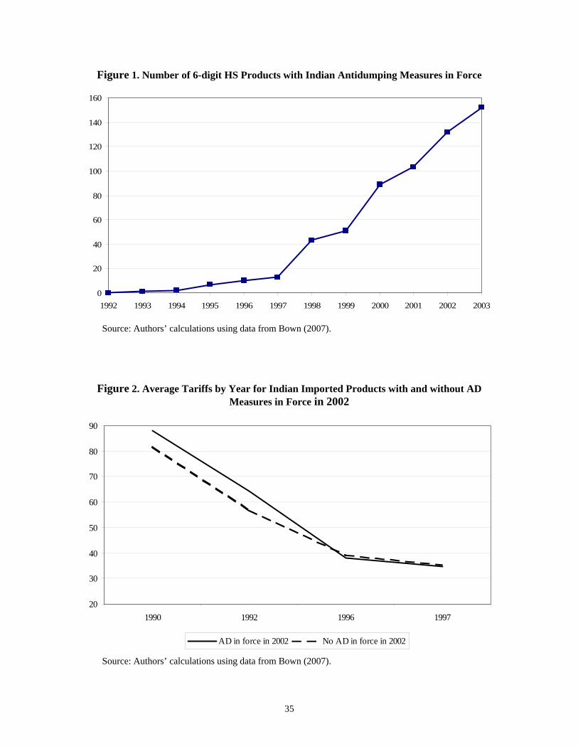
Figure 1. Number of 6-digit HS Products with Indian Antidumping Measures in Force
0
20
40
60
80
100
120
140
160
1992 1993 1994 1995 1996 1997 1998 1999 2000 2001 2002 2003
Source: Authors’ calculations using data from Bown (2007).
Figure 2. Average Tariffs by Year for Indian Imported Products with and without AD Measures in Force in 2002
20
30
40
50
60
70
80
90
1990 1992 1996 1997
AD in force in 2002 No AD in force in 2002
Source: Authors’ calculations using data from Bown (2007).
35

36
Number of AD Number of Initiations Number of SG Number of Initiations Initiations with Final AD Measure* Initiations with Final SG Measure
1992 5 5 0 01993 0 0 0 01994 6 6 0 01995 6 5 0 01996 21 21 0 01997 13 13 1 11998 28 18 5 31999 63 49 3 22000 40 33 2 12001 67 60 0 0200 3 1200 1 0200 9 1 0
Tot 16 8
* Ex ).
Year
Table 1. India’s Antidumping (AD) and Safeguard (SG) Initiations and Outcomes
2 79 563 32 204 20
al 380 295
cludes cases with only price undertakings. There was only one (in 2002
Source: Authors’ calculations using data from Bown (2007). Note that India's antidumping statute was established in 1985, although its first investigation did not take place until 1992. India's safeguard statute was established in 1997, and its first safeguard investigation took place in that year.

37
Table 2. India’s Antidumping and Safeguard Initiations and Imports by Industry: 1992-2004
Industry (3-digit ISIC) Number
of AD Initiations
Number of Final AD Measures
Number of SG
Initiations
Number of Final SG Measures
Percentage of Manufacturing
Imports (1988-2004)
Percentage of HS-6 lines with AD initiations
Percentage of 1991 imports in HS-6 lines with AD initiations
Percentage of 1992-2004 imports in HS-6 lines with
AD initiations
311- Food Products 1 0 1 0 4.7 0.3 3.1 0.3 313- Beverages 0 0 0 0 0.0 0.0 0.0 0.0 314- Tobacco 0 0 0 0 0.0 0.0 0.0 0.0 321- Textiles 9 9 0 0 1.9 0.7 4.6 8.1 322- Wearing apparel except 0 0 0 0 0.1 0.0 0.0 0.0 323- Leather products 0 0 0 0 0.4 0.0 0.0 0.0 324- Footwear except rubber or 0 0 0 0 0.0 0.0 0.0 0.0 331- Wood products except 0 0 0 0 0.1 0.0 0.0 0.0 332- Furniture except metal 0 0 0 0 0.1 0.0 0.0 0.0 341- Paper and products 9 6 1 0 2.3 7.9 48.5 36.3 342- Printing and publishing 0 0 0 0 0.5 0.0 0.0 0.0 351- Industrial chemicals 214 173 9 6 15.5 13.2 33.7 27.3 352- Other chemicals 18 17 2 2 2.7 5.9 16.8 12.8 353- Petroleum refineries 3 3 0 0 9.9 5.9 0.0 0.2 354- Misc. petroleum and coal 2 1 0 0 0.8 37.5 93.3 93.2 355- Rubber products 2 2 0 0 0.5 1.9 6.9 28.6 356- Plastic products 0 0 0 0 0.4 0.0 0.0 0.0 361- Pottery china earthenware 3 2 0 0 0.1 14.3 37.7 31.1 362- Glass and products 2 2 0 0 0.4 6.6 12.3 8.9 369- Other non-metallic mineral 9 4 0 0 0.3 11.4 1.1 14.0 371- Iron and Steel 36 25 0 0 3.9 10.0 18.3 28.9 372- Non-ferrous metals 8 1 0 0 13.6 2.0 0.9 0.3 381- Fabricated metal products 2 2 0 0 1.3 0.8 1.0 1.4 382- Machinery except electrical 17 7 1 0 12.6 1.2 3.3 2.6 383- Machinery electric 14 13 0 0 7.4 2.1 0.7 1.8 384- Transport equipment 0 0 0 0 5.0 0.0 0.0 0.0 385- Professional and scientific 4 2 0 0 2.6 3.1 1.8 3.4 390- Other manufactured 0 0 0 0 12.7 0.0 0.0 0.0
All Manufacturing 353 269 14 8 100.0 4.1 13.4 8.3
Source: Authors’ calculations using data from Bown (2007) and Nicita and Olarreaga (2007).

Table 3. Summary Statistics
a. Data used to estimate the Grossman and Helpman Model: 1990
Variable Mean Standard
Deviation Minimum Maximum
Dependent variable: Tariff 81.707 44.869 0 355
Explanatory Variables:
I x z/e 31.874 223.650 0 7448.309
z/e 46.126 351.902 0.108 11033.950
b. Data used to estimate the Grossman and Helpman Model: 2000-2002
Variable Mean Standard
Deviation Minimum Maximum
Dependent variable: Tariff 31.565 11.499 0 200.667 Tariff and AD_min 32.057 12.547 0 200.667
Tariff and AD_max 32.316 13.784 0 200.667
Explanatory Variables:
I x z/e 18.900 95.094 0 3211.348
z/e 22.064 100.091 0.042 3211.348
Notes: Number of observations is 3293.
38

Table 3. Summary Statistics
c. Data used to estimate the Binomial Probit Model (1998-2003)
Variable Expected
Sign Mean Standard
Deviation Minimum Maximum
Dependent variable:
AD initiation 0.004 0.062 0 1 Explanatory Variables:
Tariff change (1997 – 1990) b [-] -0.004 0.004 -0.027 0.004 % Tariff change (1997 – 1990) [-] -0.261 0.196 -0.991 0.298 Within industry retaliation indicator [+] 0.106 0.308 0 1 Import value a [+] 0.00001 0.0001 0 0.0159 Applied tariff b [-] 0.003 0.001 0.000 0.026 Output a [+] 0.124 0.067 0.001 0.320 Number of employees a [+] 0.004 0.003 0.0001 0.015 Number of establishments b [-] 0.614 0.404 0.030 2.291 Elasticity of import demand c [-] -0.017 0.024 -0.206 -0.0001 Indicator for previous AD initiation ? 0.009 0.096 0 1 Indicator for previous AD/SG initiation ? 0.014 0.118 0 1 Growth in output [-] 0.010 0.139 -0.825 1.495 Growth in employees [-] -0.045 0.159 -0.740 0.963 Growth in import value [+] 0.013 0.700 -8.257 7.779 Growth in import unit value [-] -0.004 0.237 -2.739 3.008 Tariff overhang [-] 0.145 0.766 -1 29
Notes: a, b, and c indicate that the variable was scaled by 10,000,000, 10,000 and 100, respectively. Number of observations is 124353.
39

Table 4. Estimation of Grossman and Helpman Model's Determinants of
Indian Use of Tariffs in 1990
Dependent variable: Applied tariff in 1990 Explanatory Variables (1) (2) (3) (4) (5) (6)
I x z/e 0.120*** 0.117*** 0.133*** 0.111*** 0.112*** 0.107 (0.027) (0.027) (0.029) (0.023) (0.027) (0.080) z/e -0.033** -0.035** -0.039*** -0.003 -0.029** -0.085 (0.014) (0.015) (0.015) (0.010) (0.014) (0.075) Constant 79.254*** 79.738*** 79.494*** 79.094*** 79.214*** 80.800*** (1.054) (1.021) (1.052) (1.058) (1.055) (0.931)
An industry is organized if number of listed groups is
At least 5 At least 6 At least 8 More than 10 More than 2 More than 1
Observations 2897 2897 2897 2897 2897 2897
Notes: Standard errors of the tobit model's estimates are in parentheses with *, **, and *** indicating statistically significant at 10%, 5% and 1% levels, respectively.
40

Table 5. Estimation of Grossman and Helpman Model's Determinants of
Indian Use of Tariffs, Antidumping and Safeguards in 2000-2002
Dependent variable is
Tariff Tariff and AD_min
Tariff and AD_max
Tariff, AD_min and SG
Tariff, AD_max and SG
Tariff and
AD_min
Tariff and
AD_max Explanatory
Variables (1) (2) (3) (4) (5) (6) (7)
I x z/e 0.074 0.186** 0.251*** 0.189** 0.254*** 0.206** 0.289*** (0.068) (0.083) (0.096) (0.084) (0.097) (0.095) (0.111) z/e -0.064 -0.179** -0.247** -0.182** -0.250*** -0.202** -0.287** (0.068) (0.083) (0.096) (0.084) (0.097) (0.096) (0.113) Constant 31.566*** 32.473*** 32.992*** 32.499*** 33.016*** 31.912*** 32.432*** (0.321) (0.391) (0.452) (0.393) (0.454) (0.523) (0.611)
-0.377 -0.858 Within industry retaliation indicator (0.732) (0.856) Growth in output 7.088** 8.027** (3.110) (3.636) Growth in employees 14.144*** 15.360*** (1.781) (2.082)
0.003 -0.024 Growth in import value (0.226) (0.264)
1.363 1.605 Growth in import unit value (1.209) (1.413)
Observations1/ 3297 3293 3293 3293 3293 3091 3091 Wald exogeneity test: p-value 0.49 0.22 0.15 0.22 0.14 0.19 0.11
Notes: Standard errors of the tobit model's estimates are in parentheses with *, **, and *** indicating statistically significant at 10%, 5% and 1% levels, respectively. 1/ Observations are cross section of 6-digit HS products averaged over 2000-2002.
41

Table 6. Estimation of Grossman and Helpman Model's Determinants of
Indian Use of Tariffs, Antidumping and Safeguards in 2000-2002: Industry Effects
Dependent variable is
Explanatory Variables Tariff and AD_min Tariff and AD_max
(1) (2)
(I x z/e) x Food products 0.307*** 0.303*** (0.051) (0.055) (I x z/e) x Tobacco 0.025** 0.026** (0.012) (0.013) (I x z/e) x Industrial chemicals 0.577*** 0.757*** (0.112) (0.122) (I x z/e) x Other chemicals 0.106*** 0.106** (0.038) (0.042) (I x z/e) x Iron and steel 0.208*** 0.205*** (0.051) (0.056) (I x z/e) x Fabricated metal products 0.179** 0.172** (0.076) (0.083) (I x z/e) x Transport equipment 0.162* 0.156 (0.098) (0.107) I x z/e 0.101 0.104 (0.066) (0.072) z/e -0.124* -0.129* (0.064) (0.070) Constant 31.269*** 31.385*** (0.480) (0.524)
Observations1/ 3289 3289
Notes: Standard errors of the tobit model's estimates are in parentheses with *, **, and *** indicating statistically significant at 10%, 5% and 1% levels, respectively. 1/ Observations are cross section of 6-digit HS products averaged over 2000-2002.
42
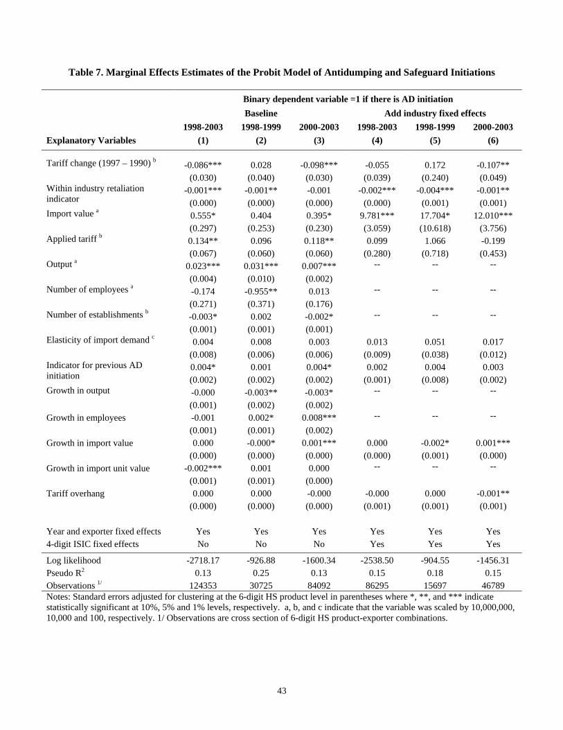
Table 7. Marginal Effects Estimates of the Probit Model of Antidumping and Safeguard Initiations
Binary dependent variable =1 if there is AD initiation
Baseline Add industry fixed effects 1998-2003 1998-1999 2000-2003 1998-2003 1998-1999 2000-2003
Explanatory Variables (1) (2) (3) (4) (5) (6)
-0.086*** 0.028 -0.098*** -0.055 0.172 -0.107** Tariff change (1997 – 1990) b
(0.030) (0.040) (0.030) (0.039) (0.240) (0.049) -0.001*** -0.001** -0.001 -0.002*** -0.004*** -0.001** Within industry retaliation
indicator (0.000) (0.000) (0.000) (0.000) (0.001) (0.001) Import value a 0.555* 0.404 0.395* 9.781*** 17.704* 12.010*** (0.297) (0.253) (0.230) (3.059) (10.618) (3.756) Applied tariff b 0.134** 0.096 0.118** 0.099 1.066 -0.199 (0.067) (0.060) (0.060) (0.280) (0.718) (0.453) Output a 0.023*** 0.031*** 0.007*** -- -- -- (0.004) (0.010) (0.002) Number of employees a -0.174 -0.955** 0.013 -- -- -- (0.271) (0.371) (0.176) Number of establishments b -0.003* 0.002 -0.002* -- -- -- (0.001) (0.001) (0.001) Elasticity of import demand c 0.004 0.008 0.003 0.013 0.051 0.017 (0.008) (0.006) (0.006) (0.009) (0.038) (0.012)
0.004* 0.001 0.004* 0.002 0.004 0.003 Indicator for previous AD initiation (0.002) (0.002) (0.002) (0.001) (0.008) (0.002) Growth in output -0.000 -0.003** -0.003* -- -- -- (0.001) (0.002) (0.002) Growth in employees -0.001 0.002* 0.008*** -- -- -- (0.001) (0.001) (0.002) Growth in import value 0.000 -0.000* 0.001*** 0.000 -0.002* 0.001*** (0.000) (0.000) (0.000) (0.000) (0.001) (0.000) Growth in import unit value -0.002*** 0.001 0.000 -- -- -- (0.001) (0.001) (0.000) Tariff overhang 0.000 0.000 -0.000 -0.000 0.000 -0.001** (0.000) (0.000) (0.000) (0.001) (0.001) (0.001) Year and exporter fixed effects Yes Yes Yes Yes Yes Yes 4-digit ISIC fixed effects No No No Yes Yes Yes
Log likelihood -2718.17 -926.88 -1600.34 -2538.50 -904.55 -1456.31 Pseudo R2 0.13 0.25 0.13 0.15 0.18 0.15 Observations 1/ 124353 30725 84092 86295 15697 46789 Notes: Standard errors adjusted for clustering at the 6-digit HS product level in parentheses where *, **, and *** indicate statistically significant at 10%, 5% and 1% levels, respectively. a, b, and c indicate that the variable was scaled by 10,000,000, 10,000 and 100, respectively. 1/ Observations are cross section of 6-digit HS product-exporter combinations.
43

Table 8. Marginal Effects Estimates of the Probit Model of Antidumping and Safeguard Initiations: Additional Robustness Tests
Binary dependent variable =1 if there is AD initiation
Change dependent variable to AD/SG
initiation Redefine tariff change variable
1998-2003 1998-1999 2000-2003 1998-2003 1998-1999 2000-2003 Explanatory Variables (1) (2) (3) (4) (5) (6)
-0.048 0.317 -0.102* -- -- -- Tariff change (1997 – 1990) b
(0.073) (0.411) (0.058) % Tariff change (1997 – 1990) -- -- -- -0.001 0.003 -0.003** (0.001) (0.005) (0.001)
-0.003*** -0.006*** -0.002** -0.002*** -0.004*** -0.001** Within industry retaliation indicator (0.001) (0.002) (0.001) (0.000) (0.001) (0.001) Import value a 13.758*** 19.690 12.731*** 9.773*** 17.798* 11.996*** (4.441) (14.953) (4.228) (3.061) (10.625) (3.752) Applied tariff b 0.159 2.383* -0.434 0.118 1.015 -0.163 (0.397) (1.447) (0.451) (0.276) (0.696) (0.452) Elasticity of import demand c 0.020 0.031 0.024* 0.013 0.050 0.018 (0.013) (0.052) (0.014) (0.009) (0.038) (0.012)
-- -- -- 0.002 0.004 0.003 Indicator for previous AD initiation (0.001) (0.008) (0.002)
0.009* 0.048 0.006** -- -- -- Indicator for previous AD/SG initiation (0.005) (0.045) (0.003)
Growth in import value 0.001** 0.001 0.001*** 0.000 -0.002* 0.001*** (0.001) (0.002) (0.000) (0.000) (0.001) (0.000) Tariff overhang -0.001 -0.001 -0.001*** -0.000 0.000 -0.001** (0.001) (0.003) (0.001) (0.001) (0.001) (0.001) Year and exporter fixed effects Yes Yes Yes Yes Yes Yes 4-digit ISIC fixed effects Yes Yes Yes Yes Yes Yes
Log likelihood -3226.15 -1267.19 -1722.16 -2538.76 -904.67 -1456.24 Pseudo R2 0.14 0.14 0.13 0.15 0.18 0.15 Observations 1/ 86889 17024 55099 86295 15697 46789 Notes: Standard errors adjusted for clustering at the 6-digit HS product level in parentheses where *, **, and *** indicate statistically significant at 10%, 5% and 1% levels, respectively. a, b, and c indicate that the variable was scaled by 10,000,000, 10,000 and 100, respectively. 1/ Observations are cross section of 6-digit HS product-exporter combinations.
44

Table 9. Estimates of the Tobit Model of Antidumping Protection
Dependent variable is
AD_min AD_max
1998-2003 1998-1999 2000-2003 1998-2003 1998-1999 2000-2003 Explanatory Variables (1) (2) (3) (4) (5) (6)
-0.345*** -0.273 -0.356*** -0.619*** -0.282 -0.698*** Tariff change (1997 – 1990)
(0.082) (0.409) (0.105) (0.163) (0.433) (0.217) -104.184*** -545.641*** -95.739*** -216.031*** -577.628*** -217.969*** Within industry retaliation
indicator (20.225) (73.781) (17.028) (39.914) (78.452) (39.089) Import value a 4.507 32.027*** -0.415 0.836 33.319*** -3.959 (4.087) (11.072) (5.125) (5.289) (11.713) (9.306) Applied tariff 0.951** 7.653*** 0.623** 1.709*** 8.212*** 1.384** (0.402) (1.538) (0.261) (0.657) (1.630) (0.555) Elasticity of import demand
2.661 30.969*** 2.339 4.820 33.029*** 4.683 (2.191) (10.462) (1.949) (3.726) (10.990) (3.743)
311.008*** 336.187*** 291.408*** 560.612*** 355.275*** 578.144*** Indicator for previous AD initiation (39.885) (35.074) (29.419) (69.749) (37.305) (79.981) Growth in import value 9.591 -31.908** 14.549** 15.224 -33.683** 25.938** (6.662) (15.724) (6.264) (12.338) (16.439) (13.005) Tariff overhang -15.117* -38.218 -11.242* -26.759 -42.491 -22.911 (8.870) (38.549) (6.479) (16.271) (40.645) (15.032) Constant -265.221*** -672.970 -305.635*** -473.935*** -714.560 -593.311*** (50.702) (0.000) (50.355) (90.214) (0.000) (111.706) Year and exporter fixed effects Yes Yes Yes Yes Yes Yes 4-digit ISIC fixed effects Yes Yes Yes Yes Yes Yes
Log likelihood -2547.68 -279.24 -2187.42 -2810.77 -281.54 -2443.10 Observations 1/ 82077 8246 47876 82077 8246 47876 Notes: Standard errors adjusted for clustering at the 6-digit HS product level in parentheses where *, **, and *** indicate statistically significant at 10%, 5% and 1% levels, respectively. a indicates that the variable was scaled by 10,000. 1/ Observations are cross section of 6-digit HS product-exporter combinations.
45
Top Related