


Languages
Pages
Legal


Topics in Number Theory and Combinatorics
By
Robert SchererDISSERTATION
Submitted in partial satisfaction of the requirements for the degree of
DOCTOR OF PHILOSOPHY
in
MATHEMATICS
in the
OFFICE OF GRADUATE STUDIES
of the
UNIVERSITY OF CALIFORNIA
DAVIS
Approved:
Professor Dan Romik (Chair)
Professor Elena Fuchs
Professor Martin Luu
Committee in Charge
2021
i
Contents
Abstract iv
Acknowledgments vi
Chapter 1. Introduction 1
1.1. Modular forms, Eisenstein series, the Jacobi theta constant, and the Weierstrass
℘-function 2
1.2. Introduction to Chapter 2: Taylor coefficients of θ3 and a conjecture of Romik 9
1.3. Introduction to Chapter 3: Regularizations of the Eisenstein series G2 and the
Weierstrass ℘-function 13
1.4. Introduction to Chapter 4: Asymptotic sharpness in tree enumeration and a conjecture
of Kuperberg 16
1.5. Introduction to Chapter 5: Expectation of the sum of binary digits in the iterated
Syracuse map 24
Chapter 2. Congruences for the Taylor coefficients of θ3 28
2.1. The auxiliary matrix (s(n, k))1≤k≤n and a recurrence relation for (d(n))∞n=0 28
2.2. Reduction of s(n, k) modulo p 29
2.3. Proof of Theorem 1.2.1 (i): The case p = 2 31
2.4. Proof of Theorem 1.2.1 (ii): Periodicity of d(n) modulo p = 5 31
2.5. Proof of Theorem 1.2.1 (iii): Vanishing of d(n) modulo p ≡ 3 (mod 4) 39
2.6. Concluding remarks 48
Chapter 3. Residual functions for shape summation of the weight-2 Eisenstein series and the
Weierstrass ℘-function 50
3.1. Proof of Theorems 1.3.1 and 1.3.2: K-summation of G2 and ℘ 50
3.2. Examples 54
ii

3.3. Concluding Remarks 54
Chapter 4. A criterion for sharpness in tree enumeration and the asymptotic number of
triangulations in Kuperberg’s G2 spider 57
4.1. Criterion for sharpness 57
4.2. Proof of Kuperberg’s Conjecture 1.4.1 67
4.3. Proof of Theorem 1.4.1: Singularity analysis 70
4.4. The case of the Lie algebra B2 88
Chapter 5. Expectation of the sum of binary digits in the iterated Syracuse map 92
5.1. Algorithms and finite-state machines 93
5.2. Proof of Theorem 1.5.2 101
5.3. Proof of Theorem 1.5.3 105
Bibliography 116
iii
Topics in Number Theory and Combinatorics
Abstract
This dissertation consists of four distinct research projects in combinatorics and number theory.
The first project, in Chapter 2, deals with the Taylor coefficients of a classical modular form, the
Jacobi theta constant θ3(τ) =∑
n∈Z e2πinτ . In particular, we prove a conjecture from [Rom20]
about periodic congruence behavior of the Taylor coefficients of θ3(τ) around the complex multi-
plication point τ = i/2. In the process we analyze an interesting two-dimensional fractal pattern,
and we prove a new result about the divisibility of the number of set partitions of a certain type.
The second project, in Chapter 3, addresses another classical modular form – the weight-two
Eisenstein seriesG2 – and the closely related Weierstrass ℘-function. The chapter can also be viewed
as an extended example in the theory of summation of series. G2 is the quintessential “quasimodular
form,” as it satisfies a unique transformation property that derives from the conditional convergence
of its defining summation, for which there are two standard regularizations that differ by a well-
known “error” term. The presence of this error term is fundamental to many further developments
in the theory of modular forms. We consider a general class of alternative regularizations of the
defining summation, and we furnish an explicit formula for the error term that arises from each
member in the class. This error term generalizes the usual one. The Weierstrass ℘-function is
similarly defined by a standard regularization of conditionally convergent summation over points
in a lattice in C, and we describe the error terms arising from alternative summations of ℘.
The third project, in Chapter 4, is in the area of asymptotic combinatorics. We prove a con-
jectured asymptotic formula of Kuperberg from the representation theory of the exceptional simple
Lie algebra G2. (Here, G2 is unrelated to the weight-2 Eisenstein series mentioned in the previous
paragraph, but we will use the symbol G2 in both Chapters 3 and 4 since the notation is standard in
both contexts and since the chapters are disjoint.) Given a non-negative sequence (an)n≥1, the iden-
tity B(x) = A(xB(x)) for generating functions A(x) = 1 +∑
n≥1 anxn and B(x) = 1 +
∑n≥1 bnx
n
determines the number bn of rooted planar trees with n+ 1 vertices such that each vertex having i
children can have one of ai distinct colors. Kuperberg proved in [Kup96] that this identity holds
in the case that bn = dim InvG2(V (λ1)⊗n), where V (λ1) is the 7-dimensional fundamental repre-
sentation of G2, and an is the number of triangulations of a regular n-gon such that each internal
iv
vertex has degree at least 6. He also observed that lim supn→∞ n√an ≤ 7/B(1/7) and conjectured
that this estimate is sharp, or, in terms of power series, that the radius of convergence of A(x) is
exactly B(1/7)/7. We prove this conjecture by introducing a new criterion for sharpness in the
analogous estimate for general power series A(x) and B(x) satisfying B(x) = A(xB(x)). Moreover
we significantly refine the conjecture by deriving an asymptotic formula for the sequence (an)n≥1.
The fourth project, in Chapter 5, is in the area of discrete probabilistic number theory. We
take a new look at the Syracuse map f : Nodd → Nodd , defined by f(x) = (3x+ 1)/2val2(3x+1). We
prove explicit formulas for the expectation of the sum of binary digits in the values of the first and
second iterates of the Syracuse map applied to a random odd integer.
v
Acknowledgments
The author would like to say a special thank-you to his advisor, Dan Romik, for teaching him
about mathematics, and many other important things in life. For introducing him to interesting
problems. For believing in him. For pushing him to excel and for his encouragement, patience, and
expertise. And generally for all of his help on projects and advising on manuscripts. It has been a
privilege to work under his mentorship.
The author would like to thank Greg Kuperberg, for his encouragement, for many helpful
conversations, and for the blessing to work on his old problem. The author would also like to thank
Michael Drmota for some critical tips about asymptotic analysis.
The author would like to thank his thesis committee, for reading this document.
The author would like to thank the first-floor administration – Tina, Sarah, and Victoria.
The author would like to thank Hamilton S., for his friendship.
The author would like to thank his parents, for their support.
And finally, the author thanks his dearest friend P, for her existence and and her uniqueness,
and for breathing life into life.
vi

CHAPTER 1
Introduction
This dissertation consists of four parts, each an individual research project, representing the
following fields: Chapters 2 and 3 deal with the theory of Modular Forms, Chapter 4 presents an
application from Analytic Combinatorics to a problem in Asymptotic Representation Theory, and
Chapter 5 discusses a problem in Discrete Probablistic Number Theory.
Chapter 2 is based on the paper Congruences modulo primes of the Romik sequence related to
the Taylor coefficients of the Jacobi theta constant θ3 [Sch21]. We prove arithmetical facts about
certain partition numbers, and in turn, statements about periodic congruences of the Taylor coef-
ficients of the classical modular form θ3. Chapter 3 is based on the paper Alternative summation
orders for the Eisenstein series G2 and Weierstrass ℘-function [RS20]. We give an explicit way to
evaluate new regularizations of the classical double summations that define G2 and ℘. Chapter 4
is based on the paper A criterion for sharpness in tree enumeration and the asymptotic number
of triangulations in Kuperberg’s G2 spider [Sch20]. We develop a new criterion for equality in an
estimate that is universal in a certain class of tree structures from graph theory. This criterion in
turn yields an estimate for the asymptotic growth rate of an important sequence from representa-
tion theory. Refinements of this asymptotic estimate are subsequently given by way of singularity
analysis. Chapter 5 is based on ongoing work with Dan Romik. We derive exact formulas for the
expected value of the sum of binary digits in values of the iterated Syracuse map. The chapters
are independent and can be read in any order.
In this introductory chapter we provide some preliminary information and describe the main
results that will follow. A comment on notation: In Chapter 3 the symbol G2 will be used to
denote the weight-2 Eisenstein series. In Chapter 4 the same symbol will be used to denote the
exceptional simple Lie Algebra G2. As these chapters are disjoint, there should not be much risk
of confusion in keeping this standard notation.
1
1.1. Modular forms, Eisenstein series, the Jacobi theta constant, and the Weierstrass
℘-function
In this section we aim to give appropriate background context to motivate the results presented
in the sequel. For a broad overview of modular forms and their applications, we recommend the
books of Zagier [Zag08], [Zag89]. For a modern algebraic introduction, culminating with the
Modularity Theorem, one should see [DS16]. For a treatment of half-integer weight modular
forms in particular, one may consult the textbook [Kob93] as well as the fundamental paper of
Shimura [Shi73], which pioneered much of the theory. Theta functions and their applications
specifically are discussed in detail in [Bel61] from a more classical perspective. In addition to
these general references, which contain the standard facts that we now describe, further citations
of more specialized results will be given below when appropriate.
Loosely speaking, a modular form is a holomorphic function defined on the upper half-plane H
that is nearly-invariant under precomposition with elements of discrete subgroups of the geometry-
preserving automorphisms of H, i.e. subgroups of SL(2,R). More precisely we have the following
definition.
Definition 1.1.1. A holomorphic modular form of weight k, for k ∈ Z, is a holomorphic function
on the upper half-plane H, satisfying the following properties:
(1) f(az+bcz+d) = (cz + d)kf(z) for all
a b
c d
∈ Γ := SL(2,Z) ,
(2) |f(z)| is bounded as Im(z)→∞.
Often one refers to such an object simply as a “modular form.” A few preliminary facts are
that the space Mk(Γ) of modular forms of a given weight k is finite dimensional, that the graded
algebra M∗(Γ) =⊕
k≥4Mk(Γ) is isomorphic to the bivariate polynomial algebra over C, and that
every modular form f has a Fourier expansion
f(τ) =∞∑n=0
ane2πinτ .
2
Furthermore, since Γ is generated by the matrices
1 1
0 1
and
0 1
−1 0
, corresponding to
the translation τ 7→ τ + 1 and the involution τ 7→ −1/τ , respectively, to check that f satisfies
the first condition above it suffices merely to check with respect to these two maps. A modular
form of weight 0 is called a modular function, and is truly Γ-invariant. A standard fact is that no
holomorphic modular functions exist – one must allow for meromorphic behavior on H or at ∞.
We will give an example below.
One can also consider modular forms with respect to a subgroup of Γ, and one can consider
half-integer weights and further generalizations involving multiplying the factor (cz + d)k in Defi-
nition 1.1.1 (the so-called “automorphy factor”) by a Dirichlet character. The precise and cumber-
some definition of a half-integer weight form is not universal, and also much more than we need,
so we merely illustrate with a classic example that will be important in Chapter 2 .
Definition 1.1.2. The Jacobi theta constant θ3 is the function defined on H by
θ3(τ) = 1 + 2∞∑n=1
e2πin2τ .
θ3 satisfies the periodicity property θ3(τ + 1) = θ3(τ), as well as the modular property
θ3
(− 1
4τ
)=
√2τ
iθ3(τ) ,
with the square root defined in terms of the principal logarithm. The modular property is a
consequence of Poisson summation applied to the Gaussian x 7→ e−πtx2
(t ∈ R+). Taken together,
these facts imply that θ3 is a “modular form of weight 1/2 on the congruence subgroup Γ0(4),”
where
Γ0(4) =
⟨1 1
0 1
,
1 0
4 1
⟩
consists of those elements in Γ for which c ≡ 0 (mod 4). This means that for any γ ∈ Γ0(4), we
have
θ3(γτ) =( cd
)εd√cτ + d θ3(τ),
where γτ = aτ+bcτ+d ,
(cd
)is the Kronecker symbol, and εd takes the value 1 when d ≡ 1 (mod 4) and −i
when d ≡ 3 (mod 4). In general, for modularity on a congruence subgroup the bounded-at-infinity
3
condition for the full modular group Γ should be supplemented with the condition that the Fourier
coefficients (an) are uniformly bounded by a polynomial as n→∞.
Returning to the setting of the full modular group Γ, we recall the following fundamental family
of examples.
Definition 1.1.3. Let k ≥ 4 be an even integer. The Eisenstein series of weight k, denoted
Gk, is defined for τ ∈ H by
(1.1) Gk(τ) =∑m,n
1
(n+mτ)k,
with the convention that the summation excludes the index (m,n) = (0, 0), where the summand is
undefined. The sum is absolutely and locally uniformly convergent, so that the order of summation
is immaterial, and it defines an analytic function on H. The sum is visibly 1-periodic, and upon
changing the variable τ 7→ −1/τ , one easily finds that Gk(−1/τ) = τkGk(τ) . In other words, Gk is
a weight-k modular form on Γ. The Fourier expansion is given by
(1.2) Gk(τ) = 2ζ(k) +2(−1)k/2(2π)k
(k − 1)!
∞∑n=1
σk−1(n)e2πinτ ,
where ζ is the Reimann zeta function and σm(n) denotes the sum of the m-th powers of the positive
divisors of n. In particular, Gk(∞) = 2ζ(k).
We can now state concretely the isomorphism mentioned above between C[x, y] and M∗(Γ),
namely by identifying x with G2 and y with G4. For an example of a modular function, consider
the famous j-invariant, which has many useful properties – the most famous of which perhaps
being the parameterization by its values of the isomorphism classes of elliptic curves over C – and
is defined on H by
j =1728E3
4
E34 − E2
6
,
where Ek := Gk/Gk(∞) for k ≥ 4. The denominator ∆ := (E34 − E2
6)/1728, called the modular
discriminant, is a modular form of weight 12 that vanishes at ∞, so that j has a pole.
Since M∗(Γ) = C[G4, G6], it is clear that no modular forms of odd weight exists for Γ, and in
fact the transformation property in Definition 1.1.1 shows directly that Gk = 0 for k ≥ 3, while for
k = 1 the sum diverges regardless of whether summation is first done over n or m. But what about
4

the case k = 2? Then (1.1) converges, but only conditionally, i.e. the value attained is sensitive to
the order of summation.
Definition 1.1.4. The weight-2 Eisenstein series G2 is the holomorphic function on H defined
by
(1.3) G2(τ) =∑m
[∑n
1
(n+mτ)2
],
summed in the indicated order over all m,n ∈ Z except for (m,n) = (0, 0), where the summand is
undefined.
Even for k = 2, this regularization of (1.1) can be expanded in a Fourier series by the same
method that leads to (1.2), and thus defines a holomorphic function on H. However, switching the
order of summation in the defining double sum (1.3) changes its value. Precisely, we have
(1.4)∑n
[∑m
1
(n+mτ)2
]=∑m
[∑n
1
(n+mτ)2
]− 2πi
τ
(with both series excluding (m,n) = (0, 0) as above). In other words, the discrepancy between the
two summation schemes is given by the “residual term” −2πi/τ .
Evaluating G2(−1/τ) in (1.3) and manipulating the double sum, one finds that (1.4) is equiv-
alent to the quasimodularity identity
(1.5) τ−2G2(−1/τ) = G2(τ)− 2πi
τ.
One way to prove the validity of (1.5) is to define a modification of G2, namely
G∗2(τ) := G2(τ)− π/Im(τ) .
Then, a somewhat tricky calculation is to show that G∗2(τ) = limε→0G2,ε(τ), where
G2,ε(τ) :=∑
(m,n)∈Z2\(0,0)
1
(mτ + n)2|mτ + n|ε.
If we assume this fact, then since G2,ε transforms like a modular form of weight 2+ε, by the absolute
convergence of the sum (resulting from the extra factor of |mτ +n|ε), one verifies by passing to the
limit that G∗2(−1/τ) = τ2G∗2(τ), and from this (1.5) follows [Zag08, p.19].
5

There is another approach that relies on first adding (not multiplying) a corrective term to the
summands in (1.3) to again obtain absolute convergence of the sum, and then exploiting the fact
that the corrective term is conditionally convergent when summed by itself [DS16, p.23]. This
trick will be explained in Chapter 3, as it is the fundamental method by which we determine the
residual terms that arise from a large class of alternative summations – see the introduction to
Chapter 3 in Section 1.3.
If it were not for the residual term −2πi/τ in (1.4) and (1.5), then G2 would be a weight-2
modular form on Γ. Far from being a deficiency, the presence of this residual term is actually
fundamental to the entire theory of modular forms and to many applications in other areas of
mathematics. For example, the modular discriminant ∆ that we introduced above can alternatively
be defined by the identityd
dzlog ∆(z) = 2πiE2(z)
and the boundary condition ∆(∞) = 0, where E2(z) = G2(z)/G2(∞) is a normalized version of
G2, whose constant term in the Fourier expansion is 1.
For an application to number theory, consider that equation (1.4) implies that the function
G2,N defined on H by
G2,N (τ) := G2(τ)−NG2(Nτ)
is an element of M2(Γ0(N)), the space of modular forms of weight 2 for Γ0(N) (defined like Γ0(4)
but with c ≡ 0 (mod N)). Since G2,2, G2,4, and θ43 are all elements of M2(Γ0(4)), which is a 2-
dimensional vector space, the linear dependence between them can be determined by comparing
the first two terms of their Fourier expansions. Upon so doing one finds that
θ3(τ)4 = −G2,4(τ)/π .
The nth Fourier coefficient of θ43 is the number of compositions of n2 as a sum of 4 squares, and
the latter identity implies that this number is 8σ1(n), which is a result of Jacobi from the 19th
century. See [DS16, Ch. 1.2] or [SS03, Ch. 10].
A recent and spectacular role for the identity (1.4) was played in the solution to the sphere-
packing problem in 8 dimensions [Via17], where it was used to construct a particularly special
6
eigenfunction of the Fourier transform. The theta constant θ3 (as well as other Jacobi theta
constants) are also involved in that construction (see also [Coh17]).
Finally, we recall the Weierstrass ℘-function.
Definition 1.1.5. The Weierstrass ℘-function is the function of two complex variables τ, z
(with the dependence on τ usually suppressed in the notation) defined as
(1.6) ℘(z) :=1
z2+
∑(m,n)∈Z2\(0,0)
[1
(z + n+mτ)2− 1
(n+mτ)2
],
for τ ∈ H and z 6∈ Zτ + Z.
The sum is absolutely convergent, precisely because of the “normalization term” 1(n+mτ)2
. In-
deed, the ℘-function is a fundamental object in the theory of elliptic functions, and the basic idea
underlying its definition (1.6) is to try to construct a doubly-periodic function with the two periods
1, τ by summing copies of a single term (for which the best choice turns out to be the meromorphic
function z−2, which has a pole of order 2 at the origin) translated over the lattice Zτ + Z. This
results in the series∑
m,n1
(z+n+mτ)2, which however is only conditionally convergent. In fact, as
we show below in Proposition 3.1.1, switching the order of summation leads to exactly the same
“residual term” as for G2:
∑m
[∑n
1
(z + n+mτ)2
]=∑n
[∑m
1
(z + n+mτ)2
]+
2πi
τ.
On the other hand, subtracting 1(n+mτ)2
from the summands in (1.6) turns the series into an
absolutely convergent one, and conveniently still ends up producing a doubly-periodic function.
We’ll have more to say about this in Section 1.3.2 of the Introduction and in Chapter 3.
The ℘-function is a fascinating construction with a natural kinship to modular forms. For one
thing, the Laurent expansion of ℘ near z = 0 is given by
℘(z) =1
z2+∞∑n=1
(2n+ 1)G2n+2(τ)zn ,
where Gm(τ) refers to the weight-m Eisenstein series defined above. Even more excitingly, for fixed
τ ∈ H we see that as (1.6) is indexed by points in the lattice L = Zτ + Z, we can think of ℘ as a
function on the torus C \ L. It is a remarkable fact that ℘ can be used to biject the torus to an
7
elliptic curve in a way that preserves the group structure of the torus. Specifically, it can be shown
that the pairs (y, x) = (℘′(z), ℘(z)) (z ∈ C \ L) biject to solutions of the equation
y2 = 4x3 − g2(τ)x− g3(τ),
where g2 = 60G4 and g3 = 140G6. The bijection is an isomorphism of groups with respect to
addition on the torus and the usual collinear addition law on elliptic curves. Moreover, two complex
tori are isomorphic if and only if the corresponding elliptic curves are isomorphic, and given any
elliptic curve y2 = 4x3 − a2x− a3 with non-vanishing cubic discriminant, i.e. a32 − 27a2
3 6= 0, there
exists a lattice L = Zτ+Z such that a2 = g2 and a2 = g3. (The modular discriminant ∆ is precisely
g32 − 27g2
3.) It follows that isomorphism classes of complex tori correspond as algebraic objects to
isomorphism classes of elliptic curves, and the conduit is precisely ℘.
We have provided more than sufficient background material to preface and motivate the next
two sections, where we will present the main results of Chapters 2 and 3, respectively. In the next
section we will look specifically at the Jacobi theta constant θ3 and at its Taylor coefficients, while
in Section 1.3 we will take a closer look at (1.4) and alternative regularizations.
8
1.2. Introduction to Chapter 2: Taylor coefficients of θ3 and a conjecture of Romik
1.2.1. The sequence (d(n))∞n=0 and our main contribution. In Chapter 2 we will establish
congruence properties of the integer-valued sequence of normalized Taylor coefficients of θ3, at
the point τ = i/2. The sequence was discovered by Romik [Rom20] and is defined below in
Definition 1.2.2. The first several terms are given by
(d(n))∞n=0 = 1, 1,−1, 51, 849,−26199, 1341999, 82018251, 18703396449, . . .
(see also [SI20]). Specifically, we will show:
Theorem 1.2.1.
(i) d(n) ≡ 1 (mod 2) for all n ≥ 0,
(ii) d(n) ≡ (−1)n+1 (mod 5) for all n ≥ 1,
(iii) if p is prime and p ≡ 3 (mod 4), then d(n) ≡ 0 (mod p) for all n > p2−12 .
This proves half of Conjecture 13 (b) in [Rom20], where the sequence (d(n)) was first intro-
duced. The half of the statement that we do not prove is that for primes p = 4k + 1, the sequence
(d(n))∞n=1 is periodic modulo p, although Theorem 1.2.1 is a specific example of this phenomenon
in the case p = 5. (This gap was filled in [GMR20] shortly after the publication in [Sch21] of the
results discussed here, thus proving the full conjecture of Romik – see Section 1.2.2.)
The sequence (d(n)) is defined in terms of the Jacobi theta constant θ3, modified from Defini-
tion 1.1.2 in the following way.
Definition 1.2.1. Let θ be the holomorphic function defined on the right half-plane x ∈ C :
Re(x) > 0 by
(1.7) θ(x) = 1 + 2
∞∑n=1
e−πn2x .
Observe that θ(x) = θ3(ix/2), and that the modular transformation of θ3 manifests for θ as
(1.8) θ
(1
x
)=√x θ(x).
9

Definition 1.2.2 (Romik [Rom20]). Define the function σ on the unit disk by
(1.9) σ(z) =1√
1 + zθ
(1− z1 + z
).
Then (d(n))∞n=0 is given by
d(n) =σ(2n)(0)
AΦn,
where Φ =Γ( 1
4)8
128π4 , and A = θ(1) =Γ( 1
4)√2π3/4 .
Thus, the numbers (d(n))∞n=0 are the Taylor coefficients, modulo trivial factors, of σ at 0. It’s
not at all clear from the definition that the numbers d(n) are integers, but this is shown to be true
in [Rom20]. Furthermore, the connection of the sequence (d(n)) to the derivatives of θ at 1 can
be made explicit:
Theorem 1.2.2 (Romik [Rom20]). For all n ≥ 0,
(1.10) θ(n)(1) = A · (−1)n
4n
bn/2c∑k=0
(2n)!(4Φ)k
2n−2k(4k)!(n− 2k)!d(k).
1.2.2. Taylor coefficients of modular forms and connection to other work. The results
presented here, which describe congruence properties of a specific integer sequence, may be viewed
in the broader context of the study of arithmetic properties of Taylor coefficients of half-integer
weight modular forms around complex multiplication points. Given a modular form f of weight k
and a CM point z ∈ H, rather than use the usual complex derivative dfdz , it is convenient to define
the Taylor expansion of f in the following way (see e.g. Ch. 5.1 in [Zag08]). Set f ′(z) = (1/2πi) dfdz
and define the differential operator ∂ by
∂f(z) = (1/2πi)f ′(z)− k
4πIm(z)f(z) .
The derivative ∂ has the advantage over f ′ of transforming like a modular form (of weight k + 2),
but at the cost of being holomorphic. Higher order derivatives ∂n are defined recursively, i.e. ∂n =
∂ ∂n−1, with the convention that one treats the factor 1/Im(z) as a constant when differentiating.
The Taylor expansion of f at z is then expressed in terms of a new variable w in the unit disk, as
(1.11) (1− w)−kf(M(w)) =
∞∑n=0
c(n)wn
n!(|w| < 1),
10

where c(n) = ∂nf(z) · (4πIm(z))n, and M is the Mobius transformation given by M(w) = z−zw1−w ,
which maps the unit disk to H with M(0) = z. In the case of θ3(z) = θ(−2iz), the Taylor coefficients
c(n) in the above expansion about the CM point z = i/2 are the sequence (d(n)) (after a proper
normalization) introduced in [Rom20] and studied here.
The congruences for (d(n)) that we consider are analogous to known congruences in the integer
weight case. For example it was shown in [LS14] that if a prime p is inert in the CM-field generated
by z, then the Taylor coefficients at z of a modular form with integer Fourier coefficients will even-
tually vanish modulo any positive power of p. In addition, the periodicity result in Theorem 1.2.1
for p = 5 has analogues for integer weight modular forms, which are known in general cases to have
periodic coefficients modulo powers of p when p is a split prime (see e.g. [DG08]). However, similar
results for weight 1/2 had not been established before the publication of the content in Chapter 2.
Shortly afterward, the following theorem appeared in [GMR20].
Theorem 1.2.3 (Guerzhoy, Mertens, Rolen (2019)). Suppose k,N ∈ N and f ∈Mk− 12(Γ1(4N))
is a modular form with algebraic Fourier coefficients, and p is a split prime in Q(τ0) for a CM
point τ0. Assume furthermore that the absolute norm of the algebraic number G2/(ζ(2k)θ3(τ0)) is
p-integral and is not divisible by p. Then there exists Ω ∈ C×, which can be chosen to depend only
on τ0 and p, such that for n1, n2 > A satisfying
n1 ≡ n2 (mod (p− 1)pA),
we have
∂n1f(τ0)/Ω2k+4n1−1 ≡ ∂n1f(τ0)/Ω2k+4n2−1 .
The modular form space Mk−1/2(Γ1(4N)) contains θ3 in the case k = 1. The transcendental
factor Ω is an algebraic multiple of the “Chowla-Selberg period” [Zag08, p. 84], which agrees with
the normalization factor AΦ used in [Rom20] in the definition of d(n). Theorems 1.2.1 and 1.2.3
together imply that Conjecture (b) of [Rom20] is true.
It is known in general [Zag08, Cor. 27] that Taylor coefficients (at a CM point) of a modular
form f (with algebraic Fourier coefficients) are algebraic multiples of powers of the Chowla-Selberg
period. What makes Romik’s result more surprising then is that (d(n))∞n=0 is a sequence of rational
integers. While even the algebraic integrality of the Taylor coefficients that we have defined above
11

is indicated (although without proof) in [Zag08] to hold generally, the degree being 1 in the case
of (d(n)) is special.
Since, as the reader will see below in Theorem 2.1.1, the integers (d(n)) can be defined recur-
sively in terms of the Taylor coefficients of a certain hypergeometric function, we point out that
recurrence relations are known in general to produce the Taylor coefficients ∂nf(τ) of modular forms
near CM points τ . This is demonstrated in [VD93] for integer-weight forms and in [GMR20] for
the half-integer weight case by a similar method, which does not bear an obvious resemblance to
the derivation in [Rom20] of a recursion for (d(n)). In particular they relate the differential opera-
tors ∂n to another differential operator, the Serre derivitive, which is defined for weight-k modular
forms f by
ϑkf(τ) := (1/2πi)f ′(τ)− k
π2G2(τ)f(τ) ,
and whose higher order iterates operate on the basis E4, E6 for M∗(Γ) in a manner that can be
described by a simple recurrence relation. The quasimodular behavior of the Eisenstein series G2
is essential for the utility of ϑk in this regard.
One last remark is that congruence properties of the Fourier coefficients of modular forms,
which can be regarded by the Fourier expansion as their derivatives at ∞, have been well-studied
since the work of Ramanujan. He famously proved, for example, that τ(n) ≡ σ11(n) (mod 691),
where σ11(n) is the sum of the 11th powers of the positive divisors of n, and τ(n) denotes the nth
Fourier coefficient of the modular discriminant ∆ introduced in Section 1.1.
12

1.3. Introduction to Chapter 3: Regularizations of the Eisenstein series G2 and the
Weierstrass ℘-function
In Chapter 3 we will show that the concept of “residual term” from (1.4) can be generalized
to a much larger class of regularizations for the series defining G2 and the Weierstrass ℘-function.
In particular, we will assign to certain compact shapes in R2 the residual term that arises from
partially summing the relevant infinite series over the integer lattice points (m,n) inside a scaled-up
copy of the shape and taking the limit of these sums as the scaling factor goes to infinity, and we
give an explicit formula for this residual term. In this introductory section we set up the relevant
definitions and state the main result.
1.3.1. Shape summation. Denote by K the class of compact sets K ⊂ R2 that are convex,
have nonempty interior and are symmetric about the x and y axes. (For simplicity we restrict the
discussion to this class of shapes, although it is possible to consider things at a greater level of
generality; see the final comment in Section 3.3.)
Definition 1.3.1. For each K ∈ K we define hK to be the real-valued function whose graph
is the upper boundary of the shape K. The function hK is necessarily compactly supported on an
interval of the form [−A,A], is an even function, and its reflection −hK is the lower boundary of
K.
Definition 1.3.2. For a shape K ∈ K and an array (am,n)m,n∈Z of complex numbers, we define
(1.12)∑K
am,n := limλ→∞
∑(m,n)∈(λK)∩Z2
am,n,
provided the limit exists. We refer to this sum as the K-summation, or shape summation with
respect to the shape K, of the array (am,n).
In the next definition we apply the concept of shape summation in a way that generalizes (1.3)
in the definition of the Eisenstein series G2.
Definition 1.3.3. If K ∈ K, we denote by G2(K, τ) the K-summation of the weight-2 Eisen-
stein series, defined as
(1.13) G2(K, τ) :=∑K
1
(mτ + n)2,
13

provided the limit defining the summation exists, and with the convention that a0,0 = 0 in (1.12),
to make allowance for the fact that the summand 1(mτ+n)2
is not defined for m = n = 0.
Definition 1.3.4. If K ∈ K and G2(K, τ) is defined, we denote by E(K, τ) the residual function
associated to K, which is defined as
E(K, τ) := G2(K, τ)−G2(τ).
With these definitions in place we have the following result, which gives an explicit formula for
the residual function.
Theorem 1.3.1. For all τ ∈ H and all K ∈ K, the limit defining G2(K, τ) exists. The residual
function E(K, τ) is given by
(1.14) E(K, τ) = 4
∫ A
0
hK(x)
τ2x2 − h2K(x)
dx
(where as before, A denotes a number for which hK is supported on [−A,A]).
1.3.2. First example: the rectangle. Let us motivate the theorem by first considering the
simplest example, namely when K is the rectangle [−c, c] × [−1, 1] with aspect ratio c, for some
c > 0. In this case, hK is the indicator function hK(x) = χ[−c,c](x). Evaluating the integral in
(1.14) gives that
E(K, τ) = G2(K, τ)−G2(τ) = −4
τtanh−1(cτ).
In terms of the principal branch of the logarithm, the latter expression is
−2
τ[log(1 + cτ)− log(1− cτ)].
Note that we can interpret the limiting case c → 0 of the shape summation (1.13) to represent a
summation with respect to an “infinitely tall and narrow” rectangle, that is, first summing over n
and then over m as in the original definition (1.3) of G2(τ). The residual function in that case should
be 0, and indeed we have that limc→0− 4τ tanh−1 (cτ) = 0. At the other extreme, we can interpret
the case c→∞ to represent summing with respect to an “infinitely long and thin” rectangle, that
is, first summing over m and then n. In this case we have that limc→∞− 4τ tanh−1 (cτ) = −2πi
τ , and
indeed this is consistent with the relation (1.4), which can now be understood as giving the residual
14

function of such long and thin rectangles. Thus we see that summing with respect to rectangles
provides a conceptual generalization of (1.4).
1.3.3. Shape summation of ℘. We can also consider shape summation for the series associ-
ated with the Weierstrass ℘-function (from Definition 1.2.2). We saw that the natural construction
to try in searching for an elliptic function was z 7→∑
m,n1
(z+n+mτ)2, but this suffers from depen-
dence on the order of summation. This phenomenon can be generalized as follows.
Definition 1.3.5. For K ∈ K and τ ∈ H, we denote by ℘(K, z) the K-summation
℘(K, z) :=∑K
1
(z + n+mτ)2(z 6∈ Zτ + Z),
provided the limit defining the summation exists. We refer to ℘(K, z) as the K-summation of the
Weierstrass ℘-function.
The next result shows that the limit defining ℘(K, z) does exists, and that ℘(K, z) is closely
related to the residual function E(K, τ) and the weight-2 Eisenstein series G2.
Theorem 1.3.2. For K ∈ K, τ ∈ H and z 6∈ Zτ + Z, ℘(K, τ) is defined and satisfies
℘(K, z) = ℘(z) +G2(τ) + E(K, τ).
15

1.4. Introduction to Chapter 4: Asymptotic sharpness in tree enumeration and a
conjecture of Kuperberg
1.4.1. Motivation from representation theory. We will analyze the sharpness of a certain
estimate that occurs naturally in the asymptotic enumeration of rooted trees (see Definition 1.4.1
below). Our motivation is a particular problem from the literature, a conjecture formulated by Ku-
perberg in his study of the representation theory of simple rank-2 Lie algebras [Kup96, Conjecture
8.2].
Specifically, set a0 = 1, and for each positive integer n, let an denote the number of triangula-
tions of a regular n-gon, such that the minimum degree of each internal vertex is 6. The sequence
begins
(an)∞n=0 = 1, 0, 1, 1, 2, 5, 15, 50, 181, 697, . . .
and is indexed in the On-Line Encyclopedia of Integer Sequences (OEIS, [SI20]) by A059710.
Next, let b0 = 1, and for each positive integer n, let bn = dimG2 Inv(V (λ1)⊗n) be the dimension
of the vector subspace of invariants in the n-th tensor power of the 7-dimensional fundamental rep-
resentation of the exceptional simple Lie algebra G2. We explain this briefly. Following [Hum72],
we recall that the Lie algebra G2 can be defined in various ways, among which are an abstract
definition as the unique semi-simple Lie algebra (up to isomorphism) corresponding to the G2 root
system, and a concrete definition as a particular 14-dimensional Lie subalgebra of the 7×7 matrices
over C. G2 has a 2-dimensional Lie subalgebra, the Cartan subalgebra, that acts via the adjoint
representation as simultaneously diagonalizable endomorphisms of G2. In general, the isomorphism
classes of finite-dimensional irreducible representations of a semi-simple Lie algebra over C with
Cartan subalgebra H are in bijection with the set Λ+ of “dominant weights,” which is a subset of
the dual of H. In the case of G2, λ1 is a particular dominant weight whose corresponding repre-
sentation V (λ1) is 7-dimensional. Taking an arbitrary tensor power of V (λ1), one can ask what is
the dimension in V (λ1)⊗n of the subspace which is annihilated by G2, where an element x ∈ G2
acts on tensor products v1⊗ v2 by x(v1⊗ v2) = xv1⊗ v2 + v1⊗xv2 and inductively by associativity
on longer tensor products. The dimension of this subspace is bn.
The sequence begins
(bn)∞n=0 = 1, 0, 1, 1, 4, 10, 35, 120, 455, 1792, . . .
16
and is indexed in OEIS as A059710.
The sequence (bn) is also known to have a combinatorial interpretation as the number of lattice
walks in the dominant Weyl chamber of the root system for G2 – a 30 sector in the triangular
lattice in R2 which serves as a geometric repsresentation for the set Λ+ above – that start and end
at the origin, subject to certain constraints on the steps [Wes07]. This type of model is not unique
to G2 or this particular representation. In general, if V is any irreducible representation of any
complex semi-simple Lie algebra L, there is a similar lattice walk model for the dimension of the
space of L-invariant n-tensors over V [GM93, Thm. 5].
Now let A(x) = 1+∑∞
n=1 anxn and B(x) = 1+
∑∞n=1 bnx
n be the ordinary generating functions
for (an)∞n=0 and (bn)∞n=0, respectively. In [Kup96, Section 8], Kuperberg proved the following
remarkable identity of formal power series:
(1.15) B(x) = A(xB(x)).
He also observed that B(x) has radius of convergence 1/7, that B (1/7) < ∞, and that by
(1.15) A(x) has radius of convergence at least (1/7)B (1/7) (see Lemma 4.1.1 below), a constant
whose numerical value he estimated to be approximately 6.811. He conjectured that this bound is
in fact an equality.
Conjecture 1.4.1 (Kuperberg, 1996 [Kup96]).
lim supn→∞
n√an = 7/B(1/7) .
1.4.2. Our main contributions. We prove Conjecture 1.4.1. Moreover, we explicitly identify
the value of Kuperberg’s constant 7/B(1/7) and go beyond the exponential growth term to establish
a true asymptotic formula for (an) and a full asymptotic expansion for (bn). The precise result is
as follows.
17
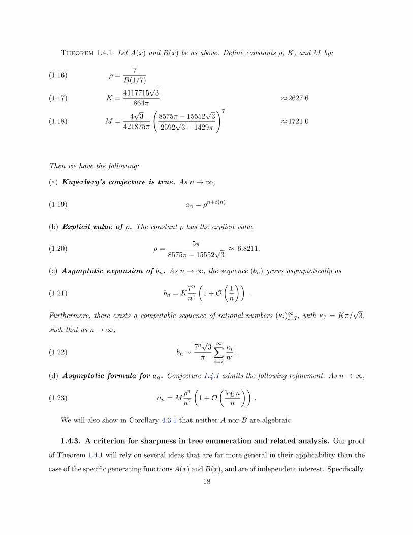
Theorem 1.4.1. Let A(x) and B(x) be as above. Define constants ρ, K, and M by:
ρ =7
B(1/7)(1.16)
K =4117715
√3
864π≈ 2627.6(1.17)
M =4√
3
421875π
(8575π − 15552
√3
2592√
3− 1429π
)7
≈ 1721.0(1.18)
Then we have the following:
(a) Kuperberg’s conjecture is true. As n→∞,
(1.19) an = ρn+o(n).
(b) Explicit value of ρ. The constant ρ has the explicit value
(1.20) ρ =5π
8575π − 15552√
3≈ 6.8211.
(c) Asymptotic expansion of bn. As n→∞, the sequence (bn) grows asymptotically as
(1.21) bn = K7n
n7
(1 +O
(1
n
)).
Furthermore, there exists a computable sequence of rational numbers (κi)∞i=7, with κ7 = Kπ/
√3,
such that as n→∞,
(1.22) bn ∼7n√
3
π
∞∑i=7
κini.
(d) Asymptotic formula for an. Conjecture 1.4.1 admits the following refinement. As n→∞,
(1.23) an = Mρn
n7
(1 +O
(log n
n
)).
We will also show in Corollary 4.3.1 that neither A nor B are algebraic.
1.4.3. A criterion for sharpness in tree enumeration and related analysis. Our proof
of Theorem 1.4.1 will rely on several ideas that are far more general in their applicability than the
case of the specific generating functions A(x) andB(x), and are of independent interest. Specifically,
18

Conjecture 1.4.1 can be viewed as an asymptotic enumeration problem in the combinatorial theory
of rooted trees, as (1.15) is a classic identity that encodes the recursive nature of these structures.
We will have more to say about this in Section 1.4.4.
In general, if A(x) = 1 +∑
n≥1 anxn and B(x) = 1 +
∑n≥1 bnx
n are ordinary generating
functions, with radii of convergence R > 0 and r > 0 respectively, and they satisfy (1.15), then the
inequality rB(r) ≤ R holds if an ≥ 0 for all n ≥ 1 (see Lemma 4.1.1). It is natural then to ask
when equality holds. We address this question in Section 4.1 and eventually arrive at a criterion
for equality in the estimate rB(r) ≤ R. A simplified version of this criterion reads as follows.
Theorem 1.4.2 (Criterion for sharpness, simplified version). With A(x), B(x), R, and r as in
the preceding paragraph, assume that an ≥ 0 for all n ≥ 1 and that gcdn ≥ 1 : an > 0 = 1. Then
bnrn 6= Θ(n−3/2) as n→∞ =⇒ R = rB(r) .
Kuperberg’s conjecture will follow from this criterion, since a formula from the character theory
of Lie algebra representations will lead us to the preliminary estimate bn/7n = Θ(n−7) for the
sequence (bn) in Conjecture 1.4.1 (see Section 4.2). For the full criterion, including some technical
details, see Theorem 4.1.3 in Section 4.1.
Another batch of concepts of general interest is the singularity analysis conducted in Section 4.3,
by which we study a new formula from [BTWZ19] for the generating function B(x) in Conjec-
ture 1.4.1 and prove the remaining parts of Theorem 1.4.1. In particular, we apply the “transfer
theorem” approach of Flajolet and Odlyzko (see Section 1.4.5). The fact that rB(r) = R for this
example (Conjecture 1.4.1) leads to rather subtle analysis in the application of this approach when
compared to the more well-studied case of rB(r) < R. Example 4.1.2 and the remark that follows
it may further clarify this perspective.
1.4.4. Simply generated trees. Let A(x) = 1 +∑
n≥1 anxn and B(x) = 1 +
∑n≥1 bnx
n be
power series satisfying (1.15). When B(x) has a positive radius of convergence, we would like to
know when the identity (1.15) of formal power series is also an identity of the complex functions
defined by these power series in a neighborhood of the origin, since then we may apply analytic
methods. A sufficient condition is non-negativity of the coefficients – see Lemma 4.1.1. We will
adopt a useful convention of setting y(x) := xB(x), whereby the identity (1.15) can be rewritten
19
as
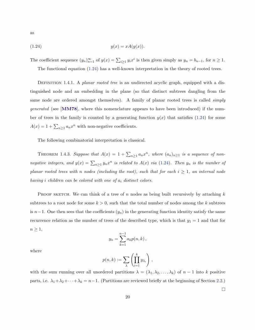
(1.24) y(x) = xA(y(x)).
The coefficient sequence (yn)∞n=1 of y(x) =∑
i≥1 yixi is then given simply as yn = bn−1, for n ≥ 1.
The functional equation (1.24) has a well-known interpretation in the theory of rooted trees.
Definition 1.4.1. A planar rooted tree is an undirected acyclic graph, equipped with a dis-
tinguished node and an embedding in the plane (so that distinct subtrees dangling from the
same node are ordered amongst themselves). A family of planar rooted trees is called simply
generated (see [MM78], where this nomenclature appears to have been introduced) if the num-
ber of trees in the family is counted by a generating function y(x) that satisfies (1.24) for some
A(x) = 1 +∑
n≥1 anxn with non-negative coefficients.
The following combinatorial interpretation is classical.
Theorem 1.4.3. Suppose that A(x) = 1 +∑
n≥1 anxn, where (an)n≥1 is a sequence of non-
negative integers, and y(x) =∑
n≥1 ynxn is related to A(x) via (1.24). Then yn is the number of
planar rooted trees with n nodes (including the root), such that for each i ≥ 1, an internal node
having i children can be colored with one of ai distinct colors.
Proof sketch. We can think of a tree of n nodes as being built recursively by attaching k
subtrees to a root node for some k > 0, such that the total number of nodes among the k subtrees
is n−1. One then sees that the coefficients (yn) in the generating function identity satisfy the same
recurrence relation as the number of trees of the described type, which is that y1 = 1 and that for
n ≥ 1,
yn =
n−1∑k=1
akp(n, k) ,
where
p(n, k) :=∑λ
(k∏i=1
yλi
),
with the sum running over all unordered partitions λ = (λ1, λ2, . . . , λk) of n − 1 into k positive
parts, i.e. λ1+λ2+· · ·+λk = n−1. (Partitions are reviewed briefly at the beginning of Section 2.2.)
20
The article [Drm04] contains several examples of (1.24) and a concise explanation of some
fundamental asymptotic results, including that the Catalan numbers occur as the sequence (yn)∞n=1
when A(x) = 1/(1− x), and in that case yn ∼ π−12 4n−1n−
32 as n→∞ (see Example 4.1.1 below).
Generalization of the functional equation (1.24) are also discussed, as well as statistical analysis
of parameters associated to trees, such as their expected number of leaves. The text [FS09, Sec.
VI.7, VII.3, VII.4] contains a broad treatment of the analytic framework for the functional equation
(1.24), which expands our discussion in 4.1, and includes asymptotic results by way of singularity
analysis applied to many natural tree examples from the literature. We give one example in the
next section.
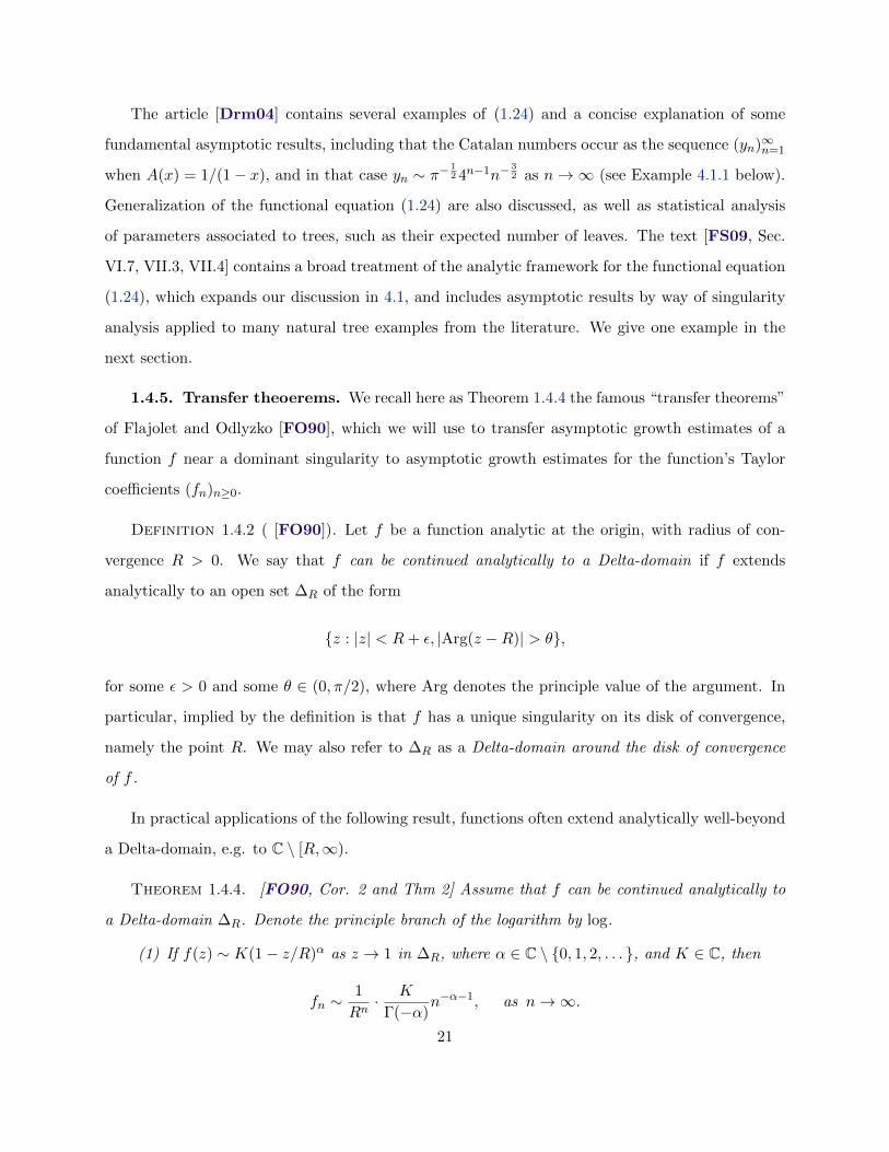
1.4.5. Transfer theoerems. We recall here as Theorem 1.4.4 the famous “transfer theorems”
of Flajolet and Odlyzko [FO90], which we will use to transfer asymptotic growth estimates of a
function f near a dominant singularity to asymptotic growth estimates for the function’s Taylor
coefficients (fn)n≥0.
Definition 1.4.2 ( [FO90]). Let f be a function analytic at the origin, with radius of con-
vergence R > 0. We say that f can be continued analytically to a Delta-domain if f extends
analytically to an open set ∆R of the form
z : |z| < R+ ε, |Arg(z −R)| > θ,
for some ε > 0 and some θ ∈ (0, π/2), where Arg denotes the principle value of the argument. In
particular, implied by the definition is that f has a unique singularity on its disk of convergence,
namely the point R. We may also refer to ∆R as a Delta-domain around the disk of convergence
of f .
In practical applications of the following result, functions often extend analytically well-beyond
a Delta-domain, e.g. to C \ [R,∞).
Theorem 1.4.4. [FO90, Cor. 2 and Thm 2] Assume that f can be continued analytically to
a Delta-domain ∆R. Denote the principle branch of the logarithm by log.
(1) If f(z) ∼ K(1− z/R)α as z → 1 in ∆R, where α ∈ C \ 0, 1, 2, . . . , and K ∈ C, then
fn ∼1
Rn· K
Γ(−α)n−α−1, as n→∞.
21
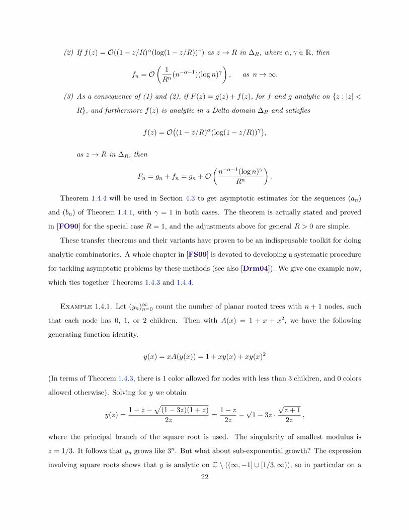
(2) If f(z) = O((1− z/R)α(log(1− z/R))γ) as z → R in ∆R, where α, γ ∈ R, then
fn = O(
1
Rn(n−α−1)(log n)γ
), as n→∞.
(3) As a consequence of (1) and (2), if F (z) = g(z) + f(z), for f and g analytic on z : |z| <
R, and furthermore f(z) is analytic in a Delta-domain ∆R and satisfies
f(z) = O((1− z/R)α(log(1− z/R))γ
),
as z → R in ∆R, then
Fn = gn + fn = gn +O(n−α−1(log n)γ
Rn
).
Theorem 1.4.4 will be used in Section 4.3 to get asymptotic estimates for the sequences (an)
and (bn) of Theorem 1.4.1, with γ = 1 in both cases. The theorem is actually stated and proved
in [FO90] for the special case R = 1, and the adjustments above for general R > 0 are simple.
These transfer theorems and their variants have proven to be an indispensable toolkit for doing
analytic combinatorics. A whole chapter in [FS09] is devoted to developing a systematic procedure
for tackling asymptotic problems by these methods (see also [Drm04]). We give one example now,
which ties together Theorems 1.4.3 and 1.4.4.
Example 1.4.1. Let (yn)∞n=0 count the number of planar rooted trees with n + 1 nodes, such
that each node has 0, 1, or 2 children. Then with A(x) = 1 + x + x2, we have the following
generating function identity.
y(x) = xA(y(x)) = 1 + xy(x) + xy(x)2
(In terms of Theorem 1.4.3, there is 1 color allowed for nodes with less than 3 children, and 0 colors
allowed otherwise). Solving for y we obtain
y(z) =1− z −
√(1− 3z)(1 + z)
2z=
1− z2z−√
1− 3z ·√z + 1
2z,
where the principal branch of the square root is used. The singularity of smallest modulus is
z = 1/3. It follows that yn grows like 3n. But what about sub-exponential growth? The expression
involving square roots shows that y is analytic on C \ ((∞,−1] ∪ [1/3,∞)), so in particular on a
22
Delta-domain around the disk of convergence z : |z| < 1/3. Furthermore, as z → 1/3 we have
y(z) =1− z −
√(1− 3z)(1 + z)
2z=
1− z2z−√
1− 3z ·√z + 1
2z
=
[1 +
3
2(1− 3z) +O(1− 3z)2
]
− (1− 3z)1/2
[√
3 +7√
3
8(1− 3z) +O(1− 3z)2
]
= 1−√
3(1− 3z)1/2 +12 + 7
√3
8(1− 3z) +O(1− 3z)3/2.
Since y(z)− 1− (1− 3z) = −√
3(1− 3z)1/2 +O(1− 3z)3/2, we see by the transfer theorem that as
n→∞,
yn =−√
3 · 3n
Γ(−1/2)n3/2+O
(3n
n2
)=
3n+1/2
2√π · n3/2
(1 +O
(1
n
)).
Moreover, by taking higher order terms in the Taylor expansions above and applying Theorem 1.4.4
to each fractional power of (1−3z), one can obtain an asymptotic formula for yn of arbitrarily high
precision.
Theorem 1.4.4 is used in Examples 4.1.1 and 4.1.2 of Chapter 4 and in proving Theorem 1.4.1
parts (c) and (d). In the case of part (d), the verification of analytic extension to a Delta-domain
is much more involved than in the other examples. We hope that the techniques that we use there
will be helpful to other researchers in future applications.
23
1.5. Introduction to Chapter 5: Expectation of the sum of binary digits in the
iterated Syracuse map
We shall make a small contribution to one of the most infamous problems in number theory,
which is to predict the trajectory of positive integers through orbits of the Collatz map.
Definition 1.5.1. The Collatz map C : N→ N is defined by
C(N) =
3N + 1 if n is odd
N/2 if n is even
Definition 1.5.2. For a function f defined on a subset S ⊂ N and for any N ∈ S, the orbit of N
(under the action of f) is defined to be the sequence of iterates (fk(N))∞k=1, where fk := f f · · ·f
(k times).
The Collatz conjecture states that every orbit assumes the value 1 eventually (and hence infin-
itely often). In every orbit of the Collatz map, odd numbers are followed by even numbers, but
not the other way around. The erratic distribution of strings of even numbers in any given orbit
is essentially what makes the Collatz map difficult to understand. This is related to the mixing
property of C when viewed as a map on the 2-adic integers Z2.
One general class of results deals with orbits of points N that are “localized in space.” That
is, if we restrict our attention to a bounded subset S of N, what can we say about limk→∞ Ck(N)?
The state of the art is the following.
Theorem 1.5.1 (Tao, 2020 [Tao20]). Let f : Z+ → R be any function with limN→∞ f(N) =∞.
Then for almost all N ∈ Z+ (in the sense of logarithmic density), f(N) exceeds the minimum value
in the orbit of N under C, i.e.
infk≥0
(Ck(N)) < f(N) .
Before this theorem emerged the best known result was that π1(N) > N0.84, where π1(N) is
defined for N ∈ Z+ as the number of positive integers less than N [KL03].
Another class of results is concerned with behavior “localized in time.” For example, one consid-
ers what can be said about C(N) or C(N)2 for all N ∈ N, either deterministically or probabilistically.
24

Our contributions are of this type. For a survey of known results, history, and methods regarding
the Collatz conjecture and related problems, one may refer to [Lag85] and [Lag10].
In Chapter 5 we will study the following modification of C, which is defined on the odd natural
numbers Nodd and neatly combines the two cases in the definition of the Collatz map. Let ω(N)
be the base-2 valuation of a positive integer N , i.e. ω(N) = supk≥0N/2k ∈ Z.
Definition 1.5.3. The Syracuse map S : Nodd → Nodd is defined by
S(N) =3N + 1
2ω(3N+1).
We will give explicit formulas for the average sum of binary digits in the first two iterates of S.
To state the precise results we first introduce some notation.
Definition 1.5.4. Define the function σ : N→ N by
σ(N) :=∞∑i=0
ti,
where N =∑∞
t=0 ti2i is the binary expansion of N (i.e. ti ∈ 0, 1 for all i). For n ∈ Z+, let Nn be
a uniform random variable with values in Nodd ∩ [1, 2n − 1]. Let (Dn)∞n=1 be the sequence defined
by
Dn := E[σ(Nn)− σ(S(Nn))],
and let (En)∞n=1 be the sequence defined by
En := E[σ(Nn)− σ(S2(Nn))].
The numbers Dn and En can be interpreted as the average loss of “complexity” (in the infor-
mation theoretic sense of nonzero bits) in the first iterate and second iterate respectively of the
Syracuse map applied to a random odd integer in [1, 2n − 1]. The initial values are as follows:
(Dn)∞n=1 = 0, 0,1
4,1
4,
5
16,
5
16,21
64,21
64, . . .
(En)∞n=1 = 0,1
2,3
4,5
8,1
2,17
32,35
64,
71
128, . . .
Moreover, we have the following explicit formulas for (Dn) and (En).
25
Theorem 1.5.2 (First iterate of S). For n ≥ 1,
(1.25) Dn =1
3− 3 + (−1)n
3× 2n.
By passing to the limit we can immediately make a simple heuristic interpretation: the image
under S of a random positive odd integer N will on average possess 1/3 fewer 1’s that N possesses
in its binary expansion.
Theorem 1.5.3 (Second iterate of S). Define the periodic sequence
(bn)∞n=0 := (−7,−5,−1, 7, 5,−8) .
For n ≥ 1,
(1.26) En =5
9+
bn9× 2n−1
.
Theorems 1.5.2 and 1.5.3 appear to generalize to higher iterates of S. For example, the following
result was discovered experimentally by Romik [RS]:
Conjecture 1.5.1 (Third iterate of S). Define the periodic sequence
(cn)∞n=0 := (17, 8, 6, 10, 9, 8,−1, 2,−6, 1,−15, 23, 8,−22,−18, 10,−3, 20).
For n ≥ 1,
E[σ(Nn)− σ(S3(Nn))] =7
9− k2 − 3k − 2cn
9× 2n.
Note that we have overloaded notation in this dissertation – the sequences (bn) and (cn) have
nothing to do with the sequences in Chapter 4.
Our approach to proving Theorems 1.5.2 and 1.5.3 in Chapter 5 is to represent the arithmetic
operation N 7→ 3N + 1 for a random odd natural number N as a finite-state machine, that is, as
a random process on a finite graph whose steps are independent Bernoulli(1/2) random variables
corresponding to the random binary digits in N . The authors of [RS] have developed a method to
prove Conjecture 1.5.1 that improves on the strategy used here for the first two iterates of S. They
replace a key conditioning step and total expectation formula (see Section 5.3.4) with a conceptually
simpler model involving linking together several finite-state machines. In theory this model can
26

be used to study higher iterates of S. The details are still in progress and will be formalized in
the future. The conditional expectation approach used here, while not generalizing well to S3 or
beyond, is perfectly adequate for handling the case of S2.
Our finite-state machine framework in Chapter 5 is not new. Similar models have been used to
study limiting behavior for orbits of certain generalizations of C to p-partite functions defined for
each N according to the congruence class of N modulo p. (See the survey [Mat10] above and the
works cited there for more information.) These maps in turn extend to ergodic maps of the p-adic
integers. We do not adopt the latter perspective here, although it may be fruitful in future work
to extend our methods to Z2 to look for a general statement about the limiting behavior of infinite
orbits of S.
27
CHAPTER 2
Congruences for the Taylor coefficients of θ3
Before beginning the proof of Theorem 1.2.1 we recall two further objects from [Rom20], an
infinite array and a recurrence relation satisfied by (d(n))∞n=0.
2.1. The auxiliary matrix (s(n, k))1≤k≤n and a recurrence relation for (d(n))∞n=0
Definition 2.1.1. Define the sequences (u(n))∞n=0 and (v(n))∞n=0 by u(0) = v(0) = 1 and the
following recurrence relations for n ≥ 1:
(2.1) u(n) = (3 · 7 · · · (4n− 1))2 −n−1∑m=0
(2n+ 1
2m+ 1
)(1 · 5 · · · (4(n−m)− 3))2 u(m) ,
(2.2) v(n) = 2n−1 (1 · 5 · · · (4n− 3))2 − 1
2
n−1∑m=1
(2n
2m
)v(m)v(n−m).
Additionally, define the infinite array s = (s(n, k))1≤k≤n as follows:
(2.3) s(n, k) =(2n)!
(2k)![z2n]
∞∑j=0
u(j)
(2j + 1)!z2j+1
2k
,
where [zn]f(z) = [zn]∑∞
n=0 cnzn denotes the nth coefficient cn in a power series expansion for f .
Finally, define r(n, k) := 2n−ks(n, k) for 1 ≤ k ≤ n.
The numbers r(n, k) were introduced in [Rom20] – and shown to be integers – along with the
following recurrence relation for d(n), which was used there to prove that (d(n)) ⊂ Z.
Theorem 2.1.1. For all pairs (n, k), 1 ≤ k ≤ n, both r(n, k) and s(n, k) are integers. Further-
more, with d(0) = 1, the following recurrence relation holds for all n ≥ 1:
(2.4) d(n) = v(n)−n−1∑k=1
r(n, k)d(k).
28

The rest of this chapter is organized as follows. In Section 2.2 we derive new formulas for
s(n, k) and s(n, k) modulo p. In Section 2.3 we give a simple proof of Theorem 1.2.1, part (i).
In Section 2.4 and Section 2.5 we give proofs of parts (ii) and (iii), respectively, based on the
expression for s(n, k) mod p derived in Section 2.2, the recursion (2.4), and a few more facts about
the congruences of (u(n)) and (v(n)).
2.2. Reduction of s(n, k) modulo p
We briefly recall some standard definitions and facts regarding integer partitions. Let n and k
be positive integers. By an unordered partition λ (of n with k parts) we mean, as usual, a tuple of
positive integers, λ = (λ1, λ2, . . . , λk), with λi ≤ λi+1 for 1 ≤ i < k, such that∑k
i=1 λi = n. The
numbers λi are the parts. We let Pn,k denote the set of unordered partitions of n with k parts, and
we let P ′n,k ⊂ Pn,k be the set of such partitions whose parts are odd numbers. For a given λ ∈ Pn,k,
we will let ci denote the number of parts (possibly zero) of λ whose value is i, for 1 ≤ i ≤ n.
Thus, the tuple c(λ) = (c1, c2, . . . , cn) gives an alternative description of λ, which we will use freely.
(Although each ci depends on λ, we choose not to reflect this dependence in the notation, in order
to keep it simple and since it will always be clear from context.) Finally, observe that∑n
i=1 ici = n,
and∑n
i=1 ci = k, for each λ ∈ Pn,k.
Lemma 2.2.1 ( [And76, pp. 215-216]). For a pair (n, k) of positive integers with n ≥ k, and
any partition λ ∈ Pn,k, define the number Nλ by
Nλ =n!∏n
i=1 i!cici!
.
Then Nλ is an integer.
In fact if S is a set with n elements, then Nλ is the number of set partitions of S into k blocks
Bi, with |Bi| ≤ |Bi+1| for 1 ≤ i < k, such that |Bi| = λi. But we will not use this interpretation.
Now we derive a formula for reduction modulo p of s(n, k).
Theorem 2.2.1. For any pair (n, k) of positive integers such that n ≥ k, we have
(2.5) s(n, k) =∑
λ∈P ′2n,2k
[(2n)!∏2ni=1 i!
cici!
2n∏i=1
u
(i− 1
2
)ci ]=
∑λ∈P ′2n,2k
[Nλ
2n∏i=1
u
(i− 1
2
)ci ].
29
Proof. We first observe that P ′2n,2k 6= ∅, since if n > k then P ′2n,2k contains the partition λ
such that c(λ) has c1 = 2k − 1, c2n−2k+1 = 1, and ci = 0 for all other i; while if n = k, then P ′2n,2kcontains λ with c(λ) = (2k, 0, . . . , 0). From (2.3) we see that
s(n, k) =(2n)!
(2k)![z2n]
∑j≥1j odd
u(j−1
2
)j!
zj
2k
=(2n)!
(2k)!
∑(j1,j2,...,j2k)
2k∏i=1
u(ji−1
2
)ji!
,(2.6)
where the sum runs over all tuples j = (j1, j2 . . . , j2k) of positive odd integers such that∑2k
i=1 ji = 2n
(in other words, over all ordered partitions of 2n into 2k odd parts). Call the set of such tuples
Λ2n,2k. Since P ′2n,2k is nonempty, so is Λ2n,2k. To each j ∈ Λ2n,2k we associate the unique unordered
partition λ ∈ P ′2n,2k obtained by ordering the ji’s in non-decreasing order, and we also associate
the tuple c(λ). We can define an equivalence relation on Λ2n,2k by calling j and j′ equivalent if
they map to the same c(λ) under this association. If j maps to c(λ) = (c1, . . . , c2n) ∈ P ′2n,2k, then
it is elementary to count that the size of the equivalence class of j is (2k)!∏2ni=1 ci!
. Furthermore, the
product∏2ki=1
u(ji−1
2
)ji!
in (2.6), as a function of (j1, . . . , j2k), is constant on equivalence classes, and
the equivalence classes are indexed by P ′2n,2k in the obvious way. Thus, we may rewrite (2.6) as
s(n, k) =(2n)!
(2k)!
∑λ∈P ′2n,2k
((2k)!∏2ni=1 ci!
2n∏i=1
u(i−1
2
)cii!ci
),
which simplifies to (2.5).
For the rest of this chapter, if x ∈ Z, and p ≥ 2 is prime, we let xp denote the congruence class
of x modulo p. In light of Lemma 2.2.1 and the fact that each u(n) is an integer, we see from (2.5)
that s(n, k) ∈ Z for 1 ≤ k ≤ n. More specifically, the summands in (2.5) are products of integers,
so we may easily reduce them modulo p to obtain the following formula for s(n, k)p.
30
Corollary 2.2.1. For any pair (n, k) of positive integers such that n ≥ k, and any prime
number p, we have
(2.7)
s(n, k)p =∑
λ∈P ′2n,2k
[ (2n)!∏2ni=1 i!
cici!
]p
2n∏i=1
[u
(i− 1
2
)ci]p
=∑
λ∈P ′2n,2k
((Nλ)p
2n∏i=1
[u
(i− 1
2
)ci]p
),
where the multiplication in parentheses is of congruence classes, as is the summation over P ′2n,2k.
2.3. Proof of Theorem 1.2.1 (i): The case p = 2
In the previous section we saw that s(n, k) = r(n, k)/2n−k is an integer for all 1 ≤ k ≤ n, which
immediately implies that r(n, k) is even. Thus, by (2.4), in order to show that d(n) is odd for all n
it suffices to show that v(n) is odd for all n. We will prove this by induction. The first few values
of v(n) are given by (v(n))∞n=0 = 1, 1, 47, 7395, . . . , which can easily be computed.
Assume now the induction hypothesis that v(m) is odd for all 1 ≤ m < n. We will write A ≡ B,
for A,B ∈ Z, to mean that A and B have the same parity. We apply the induction hypothesis to
simplify the expression in (2.2), obtaining
(2.8) v(n) ≡ 1
2
n−1∑m=1
(2n
2m
)=
1
2
[(n∑
m=0
(2n
2m
))− 2
].
Since
n∑m=0
(2n
2m
)=
1
2
[(2n∑m=0
(2n
m
))+
2n∑m=0
((2n
m
)(−1)m
)]
=1
2[22n + 0],
we see from (2.8) that v(n) ≡ 22n−2 − 1 ≡ 1, as was to be shown.
2.4. Proof of Theorem 1.2.1 (ii): Periodicity of d(n) modulo p = 5
2.4.1. A formula for r(n, k) mod 5. Corollary 2.2.1 provides a flexible way to reduce s(n, k)
– and hence r(n, k) – modulo p, and will be our main tool along with the recurrence relation (2.4)
to study the congruences of d(n) modulo primes p 6= 2. In the case p = 5, the reduction (2.7) is
31

particularly simple. Throughout this section the notation A ≡ B will be shorthand for A ≡ B
(mod 5).
Theorem 2.4.1 (Formula for r(n, k) mod 5). For 1 ≤ k ≤ n ≤ 5k the following congruences
hold mod 5:
(2.9) r(n, k) ≡
(2n)!
( 5k−n2 )!(n−k2 )!5
n−k2
if n− k is even
2(2n)!
( 5k−n−12 )!(n−k−1
2 )!5n−k−1
2
if n− k is odd
If n > 5k, then r(n, k) ≡ 0.
A graphical plot of Theorem 2.4.1 shows a compelling fractal pattern (see Figure 2.1 below).
Figure 2.1. Congruences of r(n, k) mod 5, 1 ≤ k ≤ n < 120. The rows are indexedby n, the columns are indexed by k, and the colors indicate residue classes of r(n, k)mod 5, according to the colorbar.
Before we begin the proof, we need another lemma about the sequences (u(n)) and (v(n)).
32
Lemma 2.4.1. The sequences u and v satisfy the following congruences mod 5:
(i) (v(n))∞n=0 ≡ (1, 1, 2, 0, 0, 0, 0, . . . )
(ii) (u(n))∞n=0 ≡ (1, 1, 1, 0, 0, 0, 0, . . . )
Proof. From Definition 2.1.1, one can easily calculate that the first few terms of the sequence
(u(n))∞n=0 are 1, 6, 256, 28560, 6071040. Furthermore, it is clear from (2.1) that if n ≥ 4 we have the
simplified recursion
u(n) ≡(
2n+ 1
2n− 1
)u(n− 1),
since the term (3 · 7 · 11 · · · (4n− 1))2) vanishes, as do all of the terms in the summation except for
the term corresponding to m = n− 1. Then by induction we see that u(n) ≡ 0 for all n ≥ 4.
Similarly the initial terms of the sequence (v(n))∞n=0 are 1, 1, 47, 7395, 2453425, 1399055625. For
n ≥ 2 the following congruence holds:
v(n) ≡ −1
2
n−1∑m=1
(2n
2m
)v(m)v(n−m).
So if we assume that v(k) ≡ 0 for 2 ≤ k ≤ n, then it is clear that v(n + 1) ≡ 0, and the lemma
follows by induction.
Remark 2.4.1. Whereas Theorem 2.2.1 is general for all primes, the lemma we just proved was
stated for p = 5. In fact, experimental evidence suggested that this lemma could be generalized
to the statement that u(n) and v(n) are both congruent to 0 mod p for all n ≥ p+12 , when p is a
prime congruent to 1 mod 4. This observation was subsequently verified in [Wak20] and used to
give an elementary proof of Romik’s conjecture for p = 4k+ 1, expanding on the method used here
for p = 5.
Proof of Theorem 2.4.1. In view of Lemma 2.4.1, we may restrict the class of partitions that
need to be considered in the summation appearing in (2.7). More specifically, let P3n,k ⊂ P ′n,k be
the set of partitions of n into k parts among the first three odd positive integers, 1, 3, 5. Since
u(n) vanishes mod 5 for n > 2, and therefore u(i−1
2
)vanishes mod 5 for i > 5, summands in
(2.7) that are indexed by partitions not in P32n,2k have a residue of 0 mod 5. Thus we obtain an
33
equivalent definition of s(n, k)5 to that in (2.7) if we replace the indexing set with P32n,2k and adopt
the convention that s(n, k)5 = 0 for pairs (n, k) such that P32n,2k is empty.
Furthermore, for n = 0, 1, 2, u(n) ≡ 1. Hence, u(i−1
2
)≡ 1 for i = 1, 3, 5, and if we substitute
these values of u(i−1
2
)5
into (2.7), we obtain
(2.10) s(n, k)5 =∑
λ∈P32n,2k
[(2n)!
c1!3!c3c3!5!c5c5!
]5
,
with the convention that s(n, k)5 = 0 if P32n,2k = ∅. The expression is already interesting. One
immediate implication is that if 5k < n, then r(n, k)5 = s(n, k)5 = 0, since P32n,2k is clearly empty
(see Figure 1).
To reduce the sum in (2.10) further, we recall that in the field of residues modulo 5 nonzero
elements are invertible; therefore, since we’ve shown that each summand in (2.10) is an integer, we
can replace 3! in the denominator with 1 and replace 5! = 5 · 4! with 5 · (−1) without changing the
value of the summand’s residue mod 5. Thus, we have
(2.11) s(n, k)5 =∑
λ∈P 32n,2k
[(2n)!(−1)c5
c1!c3!c5!
]5
.
Next, identify elements of P 32n,2k in the obvious way with triples (c1, c3, c5) of non-negative
integers satisfying the pair of equations∑3
i=1 ici = 2n∑3i=1 ci = 2k.
For a given pair (n, k), if we fix c5 to be some integer c, then this becomes an invertible linear
system with
c1 = 3k − n+ c , c3 = n− k − 2c.
There exists (c1, c3, c) ∈ P 32n,2k satisfying the system if and only if n ≤ 5k and
max(0, n− 3k) ≤ c ≤⌊n− k
2
⌋.
34

This allows us to rewrite (2.11) as a summation over a single index parameter:
(2.12) s(n, k)5 =
bn−k
2c∑
c=max(0,n−3k)
[(2n)!(−1)c
(3k−n+c)!(n−k−2c)!c!5c
]5
if n ≤ 5k
0 if n > 5k.
Our next step in the proof is to simplify (2.12) further by showing that the summation depends
only on the term corresponding to the largest value of the index parameter, namely c = bn−k2 c,
because all other terms are divisible by 5. This will be the content of Lemma 2.4.2 below. The
proof of the lemma will use the following formula of Legendre [Leg08], which we record here as a
theorem. For p a prime number and n a positive integer, let ωp(n) denote the p-adic valuation of n
(meaning that ωp(n) is the largest natural number α such that pα divides n), and let sp(n) denote
the sum of the digits in the base-p expansion of n.
Theorem 2.4.2 (Legendre).
ωp(n!) =n− sp(n)
p− 1.
Lemma 2.4.2. For integers 0 < k ≤ n ≤ 5k, the quantity
V (c) := ω5
((2n)!(−1)c
(3k − n+ c)!(n− k − 2c)!c!5c
),
as a function of c ∈ Z, is minimized over max(0, n− 3k) ≤ c ≤ bn−k2 c when c = bn−k2 c and for no
other values of c.
Proof. Assume k + 1 < n < 5k − 1, as otherwise there is nothing to check. Let
c ∈ max(0, n− 3k), · · · , bn−k2 c − 1, and let δ = bn−k2 c − c > 0. Then,
V (c)− V(⌊
n− k2
⌋)= V (c)− V (c+ δ) = ω5((3k − n+ c+ δ)!)− ω5((3k − n+ c)!)
+ ω5((n− k − 2(c+ δ))!)− ω5((n− k − 2c)!)
+ ω5((c+ δ)!)− ω5(c!)
+ ω5(5c+δ)− ω5(5c).
(2.13)
35
Each line of the summation contains a difference that we would like to estimate from below.
To do that, we note the general fact that if a and b are positive integers, then the estimate
ω5((a+ b)!)− ω5(a!) ≥ ω5(b!) follows from
ω5((a+ b)!) = ω5(a!) + ω5(b!) + ω5
((a+ b
a
)).
We also note that n−k−2(c+δ) = n−k−2bn−k2 c ∈ 0, 1 and n−k−2c ∈ 2δ, 2δ+1. Therefore,
we can bound from below each line in (2.13) to obtain the estimate
V (c)− V(⌊
n− k2
⌋)≥ 2ω5(δ!)− ω5((2δ + 1)!) + δ.
An application of Theorem 2.4.2 now yields
V (c)− V(⌊
n− k2
⌋)≥ 2
δ − s5(δ)
4− 2δ + 1− s5(2δ + 1)
4+ δ
= δ − s5(δ)
2+
1
4(s5(2δ + 1)− 1)
> δ − s5(δ)
≥ 0,
where the last two inequalities amount to the simple fact that for p prime, any integer k > 1 satisfies
1 < sp(k) ≤ k. We have shown that V (c) assumes its smallest value uniquely at c = bn−k2 c.
Proof of Theorem 2.4.1, continued. By the lemma, all of the summands in (2.12), except the
one indexed by c = bn−k2 c, must vanish mod 5, since they have positive valuation. The remaining
summand may or may not vanish. In any case, we have the following simplified formula for s(n, k)5,
1 ≤ k ≤ n ≤ 5k.
(2.14) s(n, k) ≡
(2n)!(−1)n−k2
( 5k−n2 )!(n−k2 )!5
n−k2
if n− k is even
(2n)!(−1)n−k−1
2
( 5k−n−12 )!(n−k−1
2 )!5n−k−1
2
if n− k is odd
Now we want to translate this into a formula for r(n, k)5 = 2n−k5 s(n, k)5. The congruence of
(n − k) modulo 4 determines the congruence of 2n−k modulo 5, as well as the sign of (−1)n−k2
(respectively (−1)n−k−1
2 ) in the case n − k is even (respectively odd). However, it turns out that
36

we need only consider parity, since 2n−k(−1)n−k2 ≡ 1, if n − k is even, and 2n−k(−1)
n−k−12 ≡ 2, if
n− k is odd. Combined with (2.14) this completes the proof of Theorem 2.4.1.
2.4.2. Proof of Theorem 1.2.1 (ii). Now that we have a nice expression for r(n, k)5, we
return to the main objective of this section, proving Theorem 1.2.1 (ii).
Lemma 2.4.3. In order to prove Theorem 1.2.1 (ii), it suffices to prove the following: For n ≥ 3,
(2.15)∑
n5≤k≤nk even
r(n, k) ≡∑
n5≤k≤nk odd
r(n, k) ≡ 0.
Proof. Assume that (2.15) holds. Then
∑n5≤k≤n
r(n, k)(−1)k =∑
n5≤k≤nk even
r(n, k)−∑
n5≤k≤nk odd
r(n, k) ≡ 0.
Subtracting r(n, n)(−1)n from the left and right sides we obtain
(2.16)∑
n5≤k≤n−1
r(n, k)(−1)k ≡ r(n, n)(−1)n+1.
A quick application of Theorem 2.4.1 shows that r(n, n) ≡ 1 for all n (in fact, it’s not hard to
deduce from (2.3) and the fact that u(1) = 1 that r(n, n) = 1 for all n), and we have also observed
above that r(n, k) ≡ 0 when 5k < n. Therefore, from (2.16) we obtain
(2.17)
n−1∑k=1
r(n, k)(−1)k ≡ (−1)n+1.
Now we prove by induction that d(n) ≡ (−1)n+1 for n ≥ 1. The cases n = 1 and n = 2 can
be checked directly, since d(1) = −1 and d(2) = 51. Also from (2.4) and Lemma 2.4.1, we see that
when n ≥ 3, the following holds:
d(n) ≡ −n−1∑k=1
r(n, k)d(k).
Thus, if n ≥ 3 and we assume the induction hypothesis that d(k) ≡ (−1)k+1 for all 1 ≤ k < n, it
follows that
d(n) ≡ −n−1∑k=1
r(n, k)(−1)k+1 ≡n−1∑k=1
r(n, k)(−1)k.
37
But the right-hand-side is congruent mod 5 to (−1)n+1, by (2.17). This verifies the induction step.
Thus, the truth of (2.15) implies that of Theorem 1.2.1 (ii).
We will now use some concepts from group theory to verify that (2.15) holds. For n a positive
integer, let Sn denote the symmetric group on n letters, and recall that every element of Sn has a
unique decomposition as a product of disjoint cycles. Let Xn be the set of elements x ∈ Sn such
that x5 = 1. For any non-negative integer k ≤ n, let Xkn denote the set of elements x ∈ Sn such
that x can be written as a disjoint product of k five-cycles and n− 5k one-cycles. Then
(2.18) Xn =
bn5c⋃
k=0
Xkn .
The connection to Theorem 2.4.1 is the following lemma.
Lemma 2.4.4. For n > 3,
(i) |X2n| =∑
n5≤k≤n
n−k even
(2n)!(5k−n
2
)!(n−k
2
)!5n−k2
,
(ii) 2(2n)(2n− 1)(2n− 2) · |X2n−3| =∑
n5≤k<n
n−k odd
2(2n)!(5k−n−1
2
)!(n−k−1
2
)!5n−k−1
2
.
Proof. Fix n > 3. For each k, 0 ≤ k ≤ n, it is not hard to show that Xkn is a conjugacy class
in Sn with cardinality
|Xkn| =
n!
(n− 5k)!k!5k
(see e.g. [DF04, Prop. 11 and Exercise 33 in Sec. 4.3]). From (2.18),
|X2n| =∑
0≤k≤ 2n5
|Xk2n| =
∑0≤k≤ 2n
5
(2n)!
(2n− 5k)!k!5k.
Therefore, to prove part (i) of the lemma, we must show that the quantity n−k2 assumes every
value in the set T1 = 0, 1, . . . , b2n5 c exactly once as k ranges over the set T2 = k : dn5 e ≤ k ≤
n, n− k even. This is not hard to see, since the change of variable k 7→ n−k2 maps n to 0, and is
linear with first difference −1/2, while both T1 and T2 have the same cardinality, as one can deduce
from a simple analysis of the cases of the congruence modulo 5 of n.
38

Similarly,
|X2n−3| =∑
0≤k≤ 2n−35
|Xk2n−3| =
∑0≤k≤ 2n−3
5
(2n− 3)!
(2n− 3− 5k)!k!5k,
so to prove part (ii) we must show that the quantity n−k−12 assumes every value in the set
0, 1, . . . , b2n−35 c exactly once as k ranges over k : dn5 e ≤ k ≤ n − 1, n − k odd. This can
be deduced from the change of variables k 7→ n−k−12 and the same type of argument as before.
Lemma 2.4.4 and Theorem 2.4.1 together imply that if n > 3 is even, then |X2n| ≡∑
n5≤k≤nk even
r(n, k),
and an integer multiple of |X2n−3| is congruent mod 5 to∑
n5≤k≤nk odd
r(n, k). Therefore, in order to verify
that (2.15) holds for n > 3 even, it suffices to show that |X2n| ≡ |X2n−3| ≡ 0. We have occasion
now to inject a dose of algebraic combinatorics into our elementary number theory, as the desired
congruence follows from a classical theorem of Frobenius (see e.g. [Fin78]).
Theorem 2.4.3 (Frobenius). Let G be a finite group whose order is divisible by a positive integer
m. Then m divides the cardinality of the set of solutions x in G to the equation xm = 1.
Since Xn is precisely the set of solutions to the equation x5 = 1 in Sn, the theorem implies that
|X2n| ≡ |X2n−3| ≡ 0 for even n > 3.
Similarly, if n > 3 is odd, then |X2n| ≡∑
n5≤k≤nk odd
r(n, k), and an integer multiple of |X2n−3| is
congruent mod 5 to∑
n5≤k≤nk even
r(n, k), and we again apply Theoerem 2.4.3 to verify (2.15). Finally, if
n = 3 we can check the validity of (2.15) by directly computing from (2.9) that r(3, 1) ≡ 4, r(3, 2) ≡
0, and r(3, 3) ≡ 1. This verifies (2.15) for all n ≥ 3 and finishes the proof of Theorem 1.2.1 (ii).
2.5. Proof of Theorem 1.2.1 (iii): Vanishing of d(n) modulo p ≡ 3 (mod 4)
Throughout this section, we a prime p congruent to 3 modulo 4. Define the constant n0 := p2−12 .
The notation A ≡ B will be shorthand for A ≡ B (mod p).
2.5.1. A vanishing theorem for u(n) and v(n). We begin with a theorem about the con-
gruences of (u(n)) and (v(n)) modulo p, similar to Lemma 2.4.1 above.
39

Theorem 2.5.1. The sequences (u(n))∞n=0 and (v(n))∞n=0 satisfy
(i)
u
(p− 1
2
)≡ 0,
(ii)
u(n) ≡ 0 for n ≥ n0,
(iii)
v(n) ≡ 0 for n > n0.
We first deduce a simple lemma that will be used repeatedly, and then we prove the theorem
in three parts.
Lemma 2.5.1. If a, b ∈ Z and p2 ≤ a < b+ p2 < 2p2, then(ab
)≡ 0.
Proof. The hypothesis implies that b ≤ p2 − 1 and a− b ≤ p2 − 1. It follows that
ωp(b!(a− b)!) =
⌊b
p
⌋+
⌊a− bp
⌋≤ a
p.
Meanwhile, since a ≥ p2
ωp(a!) ≥⌊a
p
⌋+ 1 >
a
p,
and therefore ωp((ab
))> 0.
Proof of Theorem 2.5.1 (i). By (2.1), we have
u
(p− 1
2
)= (3 · 7 · · · (2p− 3))2
−
p−12−1∑
m=0
(p
2m+ 1
)[1 · 5 · · ·
(4
(p− 1
2−m
)− 3
)]2
u(m).(2.19)
The product (3 ·7 · · · (2p−3))2 contains as factors all positive integers that are congruent to 3 mod
4 and less than 2p + 1, and p is such a number. Furthermore(pm
)≡ 0 for 1 ≤ m < p, so the sum
in (2.19) also vanishes mod p.
Proof of Theorem 2.5.1 (ii). Set n1 = 3(p+1)4 < n0. Referring to (2.1), observe that we
have 3 · 7 · · · (4n − 1))2 ≡ 0 for n ≥ p+14 , so in particular for n ≥ n0. Observe also that 0 ≡
40

1 · 5 · · · (4(n −m) − 3) if n −m ≥ n1. It follows that if n ≥ n0, we have the following truncated
summation for u(n):
(2.20) u(n) ≡n−1∑
m=n−n1+1
(2n+ 1
2m+ 1
)(1 · 5 · · · (4(n−m)− 3))2u(m).
We will also use the fact that
(2.21)
(2n+ 1
2m+ 1
)≡ 0
for n0 ≤ n ≤ n0 +n1−2 and n0−n1 +1 ≤ m ≤ n0−1, which follows from Lemma 2.5.1. Indeed,
the assumptions on n in (2.21) imply that
p2 = 2n0 + 1 ≤ 2n+ 1 ≤ 2n0 + 2n1 − 3 ≤ 2p2 − 2,
and hence
p2 +3
2(p+ 1) + 2 = 2n0 − 2n1 + 3 ≤ 2m+ 1 ≤ 2n0 − 1 = p2 − 2.
But p2 + 32(p+ 1) + 2 ≥ (2n+ 1)− p2 + 1, for n ≤ n0 + n1 − 2. In brief, Lemma 2.5.1 applies with
a = 2n+ 1 and b = 2m+ 1, verifying (2.21).
It follows that u(n0) ≡ 0, since (2.21) implies that all of the binomial coefficients in (2.20)
vanish mod p when n = n0. Now suppose that
u(n0) ≡ u(n0 + 1) ≡ · · · ≡ u(n0 + k − 1) ≡ 0,
for some k such that 1 ≤ k ≤ n1 − 2. This supposition, along with (2.20), implies that
u(n0 + k) ≡n0+k−1∑
m=n0+k−n1+1
[(2(n0 + k) + 1
2m+ 1
)
× (1 · 5 · · · (4(n0 + k −m)− 3))2u(m)
]
≡n0−1∑
m=n0+k−n1+1
[(2(n0 + k) + 1
2m+ 1
)
× (1 · 5 · · · (4(n0 + k −m)− 3))2u(m)
].
41
By (2.21) all the binomial coefficients in the sum vanish; hence u(n0 +k) ≡ 0. Since k was arbitrary,
we can conclude that u(n) ≡ 0 when n0 ≤ n ≤ n0 + n1 − 2.
Finally, by (2.20) u(n)p is a sum involving only those values of u evaluated at integers in
[n− n1 + 1, n− 1]; if these values of u vanish mod p, then so does u(n). Therefore, if one can show
that u(n) vanishes mod p for n1 − 1 consecutive values of n, then by induction u(n) must vanish
mod p for all larger n. But we’ve already shown above that u(n) vanishes for n ∈ [n0, n0 + n1− 2],
so it follows that u(n) vanishes for all n ≥ n0.
Proof of Theorem 2.5.1 (iii). Referring to the recursive definition for v(n) in (2.2), observe
that 1 · 5 · · · (4n − 3) ≡ 0 for n ≥ 3p+34 and hence for n ≥ n0. Furthermore, if n = n0 + 1 and
1 ≤ m ≤ n0, then Lemma 2.5.1 applies with a = 2n and b = 2m and hence(
2n2m
)≡ 0. Therefore,
v(n0 + 1) ≡ 0.
Now let n > n0 be arbitrary, and assume as an induction hypothesis that v(k) ≡ 0 for all
n0 < k < n. Then
(2.22) v(n) ≡ −1
2
n−1∑m=1
(2n
2m
)v(m)v(n−m).
If n ≥ 2n0, then n−m > n0 for all values of the summation index m, so by the induction hypothesis
v(n −m) vanishes mod p and so does the sum. So assume that n ≤ 2n0. Then we may restrict
the sum in (2.22) to index values m ∈ [n − n0, n0], since for other values of m either m > n0 or
n−m > n0. However, for any such m, we can apply Lemma 2.5.1 with a = 2n and b = 2m, since
p2 ≤ 2n and 2n− p2 + 1 ≤ 2m ≤ 2n0 = p2 − 1. It follows that every binomial coefficient in (2.22)
vanishes mod p and so does v(n). Induction on n > n0 completes the proof.
2.5.2. Proof of Theorem 1.2.1 (iii). We begin with a fact similar to Lemma 2.4.3, in that
it shifts the burden of proof entirely to the array (r(n, k)).
Lemma 2.5.2. If r(n, k) ≡ 0 for all pairs (n, k) such that 1 ≤ k ≤ n0 < n, then Theorem 1.2.1
(iii) is true.
Figure 2 below gives an illustration of the lemma’s hypothesis in the case p = 7.
42
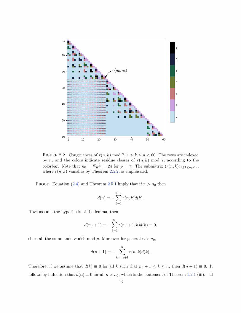
Figure 2.2. Congruences of r(n, k) mod 7, 1 ≤ k ≤ n < 60. The rows are indexedby n, and the colors indicate residue classes of r(n, k) mod 7, according to the
colorbar. Note that n0 = p2−12 = 24 for p = 7. The submatrix (r(n, k))1≤k≤n0<n,
where r(n, k) vanishes by Theorem 2.5.2, is emphasized.
Proof. Equation (2.4) and Theorem 2.5.1 imply that if n > n0 then
d(n) ≡ −n−1∑k=1
r(n, k)d(k).
If we assume the hypothesis of the lemma, then
d(n0 + 1) ≡ −n0∑k=1
r(n0 + 1, k)d(k) ≡ 0,
since all the summands vanish mod p. Moreover for general n > n0,
d(n+ 1) ≡ −n∑
k=n0+1
r(n, k)d(k).
Therefore, if we assume that d(k) ≡ 0 for all k such that n0 + 1 ≤ k ≤ n, then d(n + 1) ≡ 0. It
follows by induction that d(n) ≡ 0 for all n > n0, which is the statement of Theorem 1.2.1 (iii).
43

As we did in Section 2.4, for p = 5, we would now like to restrict the class of partitions that
we need to consider in (2.7), for p ≡ 3 (mod 4). Let P∗2n,2k ⊂ P ′2n,2k denote the set of partitions λ
whose parts are all less than p2, and such that no part of λ is equal to p, i.e. cp = 0 and ci = 0
for i ≥ p2. Theorem 2.5.1 implies that we may replace the index set in the summation (2.7) with
P∗2n,2k, since any partition λ ∈ P ′2n,2k \ P∗2n,2k must contain a part λi such that u(λi−1
2
)p
= 0 and
hence will contribute 0 to the sum. In other words,
(2.23) s(n, k)p =∑
λ∈P∗2n,2k
((Nλ)p
2n∏i=1
[u
(i− 1
2
)ci]p
),
with the convention that s(n, k)p = 0 if P∗2n,2k = ∅. The key to using formula (2.23) is the following
theorem.
Theorem 2.5.2. Let (n, k) ∈ N2 be such that 1 ≤ k ≤ n0 < n. Then
(2.24) ωp(Nλ) > 0.
The theorem implies, by (2.23), that r(n, k) = 2n−ks(n, k) vanishes mod p for 1 ≤ k ≤ n0 < n,
and in view of Lemma 2.5.2 will complete the proof of Theorem 1.2.1 (iii).
We record as a lemma a few very basic facts about arithmetic that we will use freely in the
proof of Theorem 2.5.2 to bound various quanitites. Recall that sp(n) denotes the sum of the base-p
digits in a positive integer n.
Lemma 2.5.3. If x and y are positive integers with base-p expansions x =∑
i≥0 xipi and y =∑
i≥0 yipi, then
(i) sp(x+ y) ≤ sp(x) + sp(y), with equality if and only if there are no carries when x is added
to y in base p, if and only if xi + yi ≤ p− 1 for all i.
(ii) sp(px) = sp(x) .
(iii) sp(x) = x if and only if x ≤ p− 1.
Proof of Theorem 2.5.2. Suppose λ ∈ P∗2n,2k. Then
c(λ) = (c1, c2, . . . , c2n) = (c1, c2, . . . cp−1, 0, cp+1, . . . cp2−1, 0 . . . 0).
44

For each i with 1 ≤ i < p2 we define numbers ai0 and ai1 so that ci = ai0 + ai1p is the base-p
expansion of ci, where the exponents serve as indices, and there are at most two non-zero digits in
the expansion since ci ≤ 2k < p2. Also for 1 ≤ i < p2, define bi0 and bi1 so that i = bi0 + bi1p is the
base-p expansion of i.
By Theorem 2.4.2,
ωp(Nλ)(p− 1) = ωp
((2n)!∏2ni=1 i!
cici!
)(p− 1)
= 2n− sp(2n)−2n∑i=1
[ci(i− sp(i)) + (ci − sp(ci))] .
The latter summation can be restricted to index values i ∈ [1, p2), since ci = 0 for i ≥ p2. Thus we
have
ωp(Nλ)(p− 1) = 2n− sp(2n)−p2−1∑i=1
[ci(i− sp(i)) + (ci − sp(ci))]
=
p2−1∑i=1
sp(i)ci
+
p2−1∑i=1
(sp(ci)− ci)
− sp(2n) ,
where the last equality just amounts to cancelling the terms 2n and −2n = −∑p2−1
i=1 ici. We expand
all the terms in the last line base-p, obtaining
ωp (Nλ) (p− 1) =
p2−1∑i=1
(bi0 + bi1)(ai0 + ai1p)
+
p2−1∑i=1
ai1(1− p)
− spp2−1∑
i=1
(bi0 + bi1p)(ai0 + ai1p)
.
(2.25)
45
Now we regroup terms in the right-hand side of the latter equation and apply Lemma 2.5.3, writing
ωp (Nλ) (p− 1) =
p2−1∑i=1
(bi0 + bi1)ai1p
+
p2−1∑i=1
(bi0 + bi1)ai0
+
p2−1∑i=1
ai1(1− p)
− sp
p2−1∑i=1
(bi0 + bi1p)ai0 +
p2−1∑j=1
(bj0 + bj1p)aj1p
(2.26)
≥
p2−1∑i=1
(bi0 + bi1)ai1p
− spp2−1∑
i=1
(bi0 + bi1p)ai1p
+
p2−1∑i=1
ai1(1− p)
(2.27)
+
p2−1∑i=1
(bi0 + bi1)ai0
− spp2−1∑
i=1
(bi0 + bi1p)ai0
(2.28)
≥ 0,
where we justify the last inequality as follows. The quantity in (2.28) is non-negative by Lemma 2.5.3,
and we claim that the quantity in (2.27) is also non-negative. To show that, write the quantity asp2−1∑i=1
(bi0 + bi1)ai1
− spp2−1∑
i=1
(bi0 + bi1p)ai1p
+
p2−1∑i=1
(bi0 + bi1)ai1(p− 1)
+
p2−1∑i=1
ai1(1− p)
.
The first bracketed term is non-negative by Lemma 2.5.3, and the second bracketed term is non-
negative since bi0 + bi1 ≥ 1 for all i.
Suppose now that ωp(Nλ) = 0. Then the inequality that we used to transition from (2.26)
to (2.27) and (2.28) must be an equality, and the quantity in (2.28) and the bracketed quantities
above must all vanish. These facts have a number of consequences. First, in the second bracketed
quantity, since bi0 + bi1 ≥ 1 for all i, we have ai1(bi0 + bi1) ≥ ai1 for all i. This implies that ai1 = 0, or
(b0, b1) = (1, 0), or (b0, b1) = (0, 1). Since no part of λ is equal to p, by the definition of P∗2n,2k, the
last option is only possible if ai1 = 0. We conclude that ai1 = 0 for all i ≥ 2. In view of this, the
46
identity
sp
p2−1∑i=1
(bi0 + bi1p)ai0 +
p2−1∑j=1
(bj0 + bj1p)aj1p
= sp
p2−1∑i=1
(bi0 + bi1p)ai0
+ sp
p2−1∑i=1
(bi0 + bi1p)ai1p
(from the transition from (2.26) to (2.27) and (2.28)), can be simplified to
(2.29) sp
p2−1∑i=1
(bi0 + bi1p)ai0
+ a11p
= sp
p2−1∑i=1
(bi0 + bi1p)ai0
+ a11.
Furthermore, the fact that the quantity in (2.28) vanishes implies that (2.29) can be written as
(2.30) sp
p2−1∑i=1
(bi0 + bi1p)ai0
+ a11p
=
p2−1∑i=1
(bi0 + bi1)ai0
+ a11.
We can estimate the left-hand side of (2.30) by
sp
p2−1∑i=1
(bi0 + bi1p)ai0
+ a11p
≤ spp2−1∑
i=1
bi0ai0
+ sp
pp2−1∑i=1
bi1ai0
+ a11p
= sp
p2−1∑i=1
bi0ai0
+ sp
p2−1∑i=1
bi1ai0
+ a11
≤
p2−1∑i=1
bi0ai0
+
p2−1∑i=1
bi1ai0
+ a11,
(2.31)
which is just the right-hand side of (2.30), we must have equality throughout (2.31). It follows that
sp
p2−1∑i=1
bi0ai0
+ sp
p2−1∑i=1
bi1ai0
+ a11
=
p2−1∑i=1
bi0ai0
+
p2−1∑i=1
bi1ai0
+ a11,
and hence, by Lemma 2.5.3 (iii), we see that
(2.32)
p2−1∑i=1
bi0ai0
≤ p− 1 , and
p2−1∑i=1
bi1ai0
+ a11 ≤ p− 1.
47

Recalling that 2n =∑p2−1
i=1 ici, and that ai1 = 0 for all i ≥ 2, we see from (2.32) that
2n = a11p+
p2−1∑i=1
(bi0 + bi1p)ai0
=
p2−1∑i=1
bi0ai0
+ p
p2−1∑i=1
bi1ai0
+ a11
≤ (p− 1) + p(p− 1)
= p2 − 1.
In conclusion, the supposition above that ωp(Nλ) = 0 led us to the statement that 2n ≤ p2− 1,
or equivalently n ≤ n0. Since the hypothesis of Theorem 2.5.2 assumes n > n0, we have proved the
theorem’s contrapositive.
2.6. Concluding remarks
Remark 2.6.1. Theorem 2.5.2 was custom-made to use in conjunction with Lemma 2.5.2.
However, the odd parity of the parts in P ∗2n,2k was never used in the proof, nor was the congruence
of p modulo 4, nor were the even parity of the number of parts (2k) or the value (2n) of the integer
to which they summed. In fact, the reader will see that the same proof goes through to verify the
following general combinatorial result.
Theorem 2.6.1. Let p > 0 be a prime number. Let (n, k) ∈ N2 be such that 1 ≤ k < p2 ≤ n,
and let λ be a partition of n into k parts such that all the parts are less than p2 and no part is equal
to p. Then p divides Nλ.
As our proof is elementary number theoretic, it would be interesting to give a combinatorial
proof or an algebraic proof of this theorem. We leave as an open problem the challenge of doing
so. We also pose the problem of generalizing to the higher-power case, where 1 ≤ k < pα ≤ n for
α > 2, e.g. by finding appropriate restrictions on the parts in λ to ensure that Nλ is divisible by
pα−1.
Remark 2.6.2. The inspiration for our proof of Theorem 1.2.1 (iii) was supplied by Figure 2,
from which it seems obvious that s(n, k) vanishes modulo p for 1 ≤ k ≤ n0 < n, at least in the
48
case p = 7. It is natural then to ask why the results for p = 5 and p = 4k + 3 are so different.
Surely the difference should be reflected somewhere in the proofs of the respective statements. The
most important difference is that u(2)5 = u(
5−12
)5
= 1, whereas u(p−1
2
)p
= 0 for p = 4k + 3.
Consequently, there exist partitions in P32n,2k that index non-vanishing summands in (2.7), and
indeed those partitions with the largest possible number of 5’s are the important ones. On the
other hand, when p = 4k + 3, partitions in P ′2n,2k with parts equal to p do not contribute to the
sum in (2.7) at all. It seems plausible then that a statement similar to Theorem 2.5.1 that is general
for powers pα of primes p = 4k + 3 would exist and be useful in conjunction with a higher-power
version of Theorem 2.6.1 in proving that d(n) eventually vanishes modulo pα.
49

CHAPTER 3
Residual functions for shape summation of the weight-2
Eisenstein series and the Weierstrass ℘-function
We continue from Section 1.3, where we defined the notion of shape summation and stated our
main result, Theorem 1.3.1. This chapter is organized as follows. In Section 3.1 we give the proof
of Theorem 1.3.1. In Section 3.1 we discuss shape summation for the Weierstrass ℘-function and
prove Theorem 1.3.2. In Section 3.2 we demonstrate our notion of residual function with some
concrete examples, and in Section 3.3 we make some concluding remarks.
3.1. Proof of Theorems 1.3.1 and 1.3.2: K-summation of G2 and ℘
A key ingredient in the proof is the following Lemma 3.1.1, which shows that the right-hand
side of (1.14) is the K-summation of a different series than (1.13), which has the advantage of being
a telescoping series in the summation index n. In proving Theorem 1.3.1, we will use this series to
write G2(τ) as a series that converges absolutely, which will allow us to compare it with G2(K, τ)
and show that the series in Lemma 3.1.1 coincides with the residual function E(K, τ).
Lemma 3.1.1. Let K ∈ K be a shape with corresponding function hK , supported on [−A,A].
Then ∑K
(1
mτ + n− 1
mτ + n+ 1
)= 4
∫ A
0
hK(x)
τ2x2 − h2K(x)
dx,
where we exclude summands corresponding to m = 0, that is, we set a0,n = 0 for all n in (1.12).
Proof. For brevity of notation, we set h = hK for the rest of the proof. To evaluate the sum
in the lemma, we rewrite it as
∑K
(1
mτ + n− 1
mτ + n+ 1
)= lim
λ→∞
∑−λA≤m≤λA
m 6=0
∑−λh(m/λ)≤n≤λh(m/λ)
(1
mτ + n− 1
mτ + n+ 1
).
(3.1)
50
After telescoping the inner summation, this becomes
limλ→∞
∑−λA≤m≤λA
m 6=0
( 1
mτ − bλh(mλ )c− 1
mτ + bλh(mλ )c+
1
mτ + bλh(mλ )c− 1
mτ + bλh(mλ )c+ 1
)
= limλ→∞
∑−λA≤m≤λA
m 6=0
[(2bλh(mλ )c
m2τ2 − bλh(mλ )c2
)+
1
(mτ + bλh(mλ )c)(mτ + bλh(mλ )c+ 1)
]
= 2 limλ→∞
∑1≤m≤λA
(2bλh(mλ )c
m2τ2 − bλh(mλ )c2
)
= 4 limλ→∞
1
λ
∑1≤m≤λA
(λ−1bλh(mλ )c
λ−2m2τ2 − λ−2bλh(mλ )c2
).
Since, λ−1bλh(mλ )c ∼ h(mλ ) and λ−2bλh(mλ )c2 ∼ h(mλ )2 as λ→∞, the above limit is the same
as the limit of a Riemann sum,
4 limλ→∞
1
λ
∑1≤m≤λA
(h(mλ )
λ−2m2τ2 − h2(mλ )
),
which is the integral in the lemma.
We now observe that
∑m6=0
[∑n∈Z
(1
mτ + n− 1
mτ + n+ 1
)]= 0.
To see this, note that for any m 6= 0, the inner sum converges absolutely (since the summands are
O(1/n2) as n→∞), and is equal to
limN→∞
N−1∑n=−N
(1
mτ + n− 1
mτ + n+ 1
)= lim
N→∞
(1
mτ −N− 1
mτ +N
)= 0.
Thus, we can write G2(τ) in a different form, namely
G2(τ)−∑n6=0
1
n2=∑m6=0
[∑n∈Z
1
(n+mτ)2
]
=∑m6=0
[∑n∈Z
1
(n+mτ)2
]−∑m6=0
[∑n∈Z
(1
mτ + n− 1
mτ + n+ 1
)]
=∑m6=0
[∑n∈Z
1
(mτ + n)2(mτ + n+ 1)
].
51

The latter series has the advantage of converging absolutely by comparison with∑
m
∑n
1(mτ+n)3
(see Lemma 1.1 in [2]).
Next we observe, still setting h = hK , that Definition 1.3.3 can be expressed as
(3.2) G(K, τ) =∑n6=0
1
n2+ limλ→∞
∑−λA≤m≤λA
m 6=0
∑−λh(m/λ)≤n≤λh(m/λ)
1
(mτ + n)2.
By combining (3.1) and (3.2) , we obtain
G2(K, τ)−∑n 6=0
1
n2−∑K
(1
mτ + n− 1
mτ + n+ 1
)
= limλ→∞
∑−λA≤m≤λA
m6=0
∑−λh(m/λ)≤n≤λh(m/λ)
(1
(mτ + n)2− 1
mτ + n+
1
mτ + n+ 1
)
= limλ→∞
∑−λA≤m≤λA
m 6=0
∑−λh(m/λ)≤n≤λh(m/λ)
1
(mτ + n)2(mτ + n+ 1)
=∑m6=0
[∑n∈Z
1
(mτ + n)2(mτ + n+ 1)
],
where in the last equality we have appealed to absolute convergence to justify rearranging the
series. From the above we see that
E(K, τ) = G2(K, τ)−G2(τ) =∑K
(1
mτ + n− 1
mτ + n+ 1
).
When we replace the latter sum with the integral expression from the lemma, the proof of Theo-
rem 1.3.1 is complete.
We discussed after Definition 1.6 how thinking about elliptic functions and the motivation
behind the definition of ℘ leads one to consider different orders of summation for the conditionally
convergent infinite series∑
m,n1
(z+n+mτ)2, in a way that is precisely analogous to the situation with
G2. It turns out, as we see in Theorem 1.3.2, that this leads to exactly the same notion of “residual
function” that we already defined. As with G2, the two most obvious orders for summing the series
are as iterated summations with respect to the summation indices m,n, in the two possible orders.
The comparison between these two orders of summation is given in the following result, which is a
52
more explicit version of a result stated implicitly as part of an exercise on p. 281 of [SS03], and is
analogous to (1.4).
Proposition 3.1.1. For z 6∈ Zτ +Z, the following identity holds, where summations are in the
indicated order, over all pairs (m,n) ∈ Z2.
∑m
[∑n
1
(z + n+mτ)2
]=∑n
[∑m
1
(z + n+mτ)2
]+
2πi
τ.
Proof. We rewrite the sum defining ℘(z) in the following way, excluding from the summations
the terms corresponding to m = n = 0.
℘(z) =1
z2+∑m
[∑n
(1
(z + n+mτ)2− 1
(mτ + n)2
)]
=1
z2+∑m
[∑n
1
(z + n+mτ)2
]−∑m
[∑n
1
(mτ + n)2
]
=1
z2+∑m
[∑n
1
(z + n+mτ)2
]−G2(τ).
Meanwhile, we can sum the function ℘(z) in the reverse order, by absolute convergence, obtaining
℘(z) =1
z2+∑n
[∑m
(1
(z + n+mτ)2− 1
(mτ + n)2
)]
=1
z2+∑n
[∑m
1
(z + n+mτ)2
]−∑n
[∑m
1
(mτ + n)2
]
=1
z2+∑n
[∑m
1
(z + n+mτ)2
]−G2(τ) +
2πi
τ,
by (1.4). The proposition follows by comparing these two expressions for G2(τ).
Recall that in Chapter 1 we defined general shape summation for the series associated with the
℘-function by
℘(K, z) :=∑K
1
(z + n+mτ)2(z 6∈ Zτ + Z),
for K ∈ K and τ ∈ H. We prove Theorem 1.3.2 now, which asserted the identity
℘(K, z) = ℘(z) +G2(τ) + E(K, τ).
53

Proof of Theorem 1.3.2. By absolute convergence of the sum defining ℘(z), we can sum
over the integer lattice points in any order without changing the function’s value. Therefore,
℘(z) =∑K
[1
(z + n+mτ)2− 1
(n+mτ)2
],
where a0,0 = 1z2
in (1.12). Thus,
℘(z) =∑K
1
(z + n+mτ)2−∑K
1
(n+mτ)2
= ℘(K, z)−G2(K, τ)
= ℘(K, z)− (G2(τ) + E(K, τ)).
3.2. Examples
The integral in the explicit formula (1.14) can sometimes be evaluated in closed form. Here are
a few examples.
(1) Rectangle. As we saw in Section 1.3.2, the residual function for the rectangle [−c, c]× [−1, 1]
with aspect ratio c > 0 is E(K, τ) = − 4τ tanh−1(cτ).
(2) Disk. When K is the disk of radius 1 centered at the origin, we have hK(x) =√
1− x2,
x ∈ [−1, 1]. According to Theorem 1.3.1, we have
E(K, τ) = 4
∫ 1
0
√1− x2
τ2x2 − (1− x2)dx =
−2πi
τ + i.
(3) Diamond. For the last example we let K be the diamond x + iy : |x| + |y| ≤ 1. Then
hK(x) = 1− |x|, x ∈ [−1, 1]. We have
E(K, τ) = 4
∫ 1
0
1− xτ2x2 − (1− x)2
dx =4 log(−iτ) + 2πiτ
1− τ2,
where log denotes the principal branch of the logarithm.
3.3. Concluding Remarks
(1) We have constructed a large family of examples of natural rearrangements of conditionally
convergent series. Our explicit formula (1.14) for the residual function E(K, τ) provides a
54

general way to evaluate the discrepancy between any rearrangement in the family we considered
and the “default” ordering of the series, thus generalizing the well-known relation (1.4) and
its equivalent version (1.5). As we mentioned before, this quasimodularity relation (1.5), while
being an example of “bad behavior” from the point of view of infinite series, is actually a useful
and important property of G2, forming the basis for the study of many of its properties as well
as the properties of additional functions in complex analysis and the theory of modular forms
that are constructed using G2 as a building block. In view of the importance of (1.5), it is
interesting to wonder whether (1.14) might similarly provide fresh insight into some questions
about modular forms that are of independent interest.
(2) Also related to (1.5) is the observation that for any K ∈ K, if K is symmetric about the line
y = x, then the residual function E(K, τ) satisfies a similar functional equation, namely
(3.3) E(K, τ) = τ−2E(K,−1/τ)− 2πi
τ,
which differs from the equation for G2(τ) only in the sign of the 2πiτ term. This can be derived
as follows. Given a shape K, we let KT be the shape obtained by reflecting K about the line
x = y.
Replacing τ with −1/τ in the K-summation of G2(K, τ), one obtains
G(K,−1/τ) = τ2G(KT , τ)
= τ2(G2(τ) + E(KT , τ)).
Meanwhile, the functional equation for G2(τ) implies that
G(K,−1/τ) = G2(−1/τ) + E(K,−1/τ)
= τ2G2(τ)− 2πiτ + E(K,−1/τ).
Equating these two expressions for G(K,−1/τ) and subtracting the term τ2G2(τ) from both
sides gives
E(KT , τ) = τ−2E(K,−1/τ)− 2πi
τ.
If K is symmetric about y = x, then KT = K, so (3.3) holds.
55

(3) We saw how a shape K ∈ K gives rise to residual functions, which are computed as a kind of
integral transform of the associated bounding function hK . It seems natural to try to reverse
this correspondence and ask which holomorphic functions f : H→ C occur as residual functions
for shapes in K. We leave this as an open problem.
(4) Finally, we note that one can consider summation with respect to shapes in greater levels of
generality. In particular, one could expand the class of shapes K by relaxing the symmetry
conditions, the condition of compactness, or both. We leave to the interested reader to work
out the details of such generalizations.
56
CHAPTER 4
A criterion for sharpness in tree enumeration and the asymptotic
number of triangulations in Kuperberg’s G2 spider
This chapter is organized as follows.
In Section 4.1 we continue with our discussion from Section 1.4.4 about simply generated trees
and identity (1.24) – y(x) = xA(y(x)). We state and prove our asymptotic sharpness criterion,
Theorem 4.1.3, of which Theorem 1.4.2 is a corollary. We also give a pair of examples.
In Section 4.2 we prove Kuperberg’s conjecture (1.19) way of 1.4.2. As mentioned in Chap-
ter 1, a preliminary step is to obtain a growth estimate for the sequence (bn). This we do in
Proposition 4.2.1 by way of saddle-point analysis of a known formula from the character theory of
Lie algebra representations.
In Section 4.3 we prove the remaining parts of Theorem 1.4.1. The constant ρ is evaluated
in Proposition 4.3.1, and the remainder of the section contains a detailed singularity analysis that
leads to (1.22) and (1.23). An outline of the method is given at the beginning of the section. We
will also obtain along the way another proof of Conjecture 1.4.1 that is independent of the first one
in Section 4.2.
In Section 4.4 we apply the sharpness criterion Theorem 4.1.3 (or Theorem 1.4.2) to the Lie
algebra B2 and the asymptotic counting of the quadrangulations in the B2 spider.
4.1. Criterion for sharpness
We pick up from Section 1.4.4 and the identity (1.24) – y(x) = xA(y(x)). Throughout this
chapter, when thinking of power series as analytic functions we will use the variable z or w, e.g.
writing y(z). On the other hand, writing y(x) will emphasize thinking of formal power series
combinatorially, without considerations of convergence or analytic continuation. This distinction
is more psychological than mathematical and could also just be ignored.
57
4.1.1. Preliminary lemmas.
Lemma 4.1.1. Let A(x) = 1 +∑
i≥1 aixi and y(x) =
∑i≥1 yix
i be power series over R related
by (1.24), with ai ≥ 0 for all i ≥ 1 . Then yi ≥ 0 for all i. Let R be the radius of convergence of
A, and let r denote the radius of convergence of y. Then R > 0 iff r > 0, and
(4.1) y(z) = zA(y(z))
for z ∈ Ω = z ∈ C : |z| < r. Also, y(r) ≤ R, including when y(r) =∞.
Remark 4.1.1. Notice that neither r nor R are required to be finite in the lemma. However,
it is easy to see that if an ≥ 1 for all large enough n, then R ≤ 1, so that y(r) ≤ 1 by the lemma,
and hence r <∞.
Proof. Given A(x), the Lagrange Inversion Theorem [Sta99, Ch. 5.4] implies that the unique
power series solution to (1.24) is given by
(4.2) yi =1
i[xi−1](A(x)i),
for all i ≥ 1, where [xi]f(x) denotes the i’th coefficient of a power series f(x). The right-hand side
is non-negative, so yi ≥ 0 for all i.
To prove the next part, suppose R > 0 and consider the function F (z, w) = w − zA(w), which
is analytic for z ∈ C and |w| < R. Then Fw = 1 − zA′(w) is non-zero at (0, 0), so that by the
implicit function theorem there exists a function y, analytic near the origin, with F (z, y(z)) = 0.
By (4.2), y = y, which shows that r > 0.
Now assume r > 0 and let z be a non-negative number in Ω. Then
zA(y(z)) = z
∞∑i=0
ai ∞∑j=1
yjzj
i =
∞∑i=1
∞∑j=i
(cijzj) =
∞∑j=1
[(j∑i=1
cij
)zj
],
where cij = ai[xj−1]
(∑∞k=1 ykx
k)i
, and the interchange of the order of summation is permitted
since each cij is non-negative. The fact that y(z) =∑∞
j=1
[(∑ji=1 cij
)zj]
is just a reformulation
of (1.24). So zA(y(z)) = y(z) < ∞. Thus, the double sum above is absolutely convergent on Ω,
and (4.1) is valid on Ω.
58
Next, since the coefficients of y(x) are non-negative, y maps [0, r) bijectively to [0, y(r)). There-
fore, if 0 < |z| < y(r), then |z| = y(w) for some w ∈ (0, r), and A(|z|) = y(w)/w <∞. So R ≥ y(r).
In particular R > 0, since y1 = 1 and hence y(r) ≥ r. The lemma is trivial when r = R = 0.
As mentioned in the proof, for a generating function A(x) = 1+∑
n≥1 anxn, the unique solution
y(x) to (1.24) is given by formula (4.2). When furthermore the an’s are non-negative, we associate
to A another function ψ, defined by
(4.3) ψ(z) :=z
A(z)
on the set z : |z| < R and A(z) 6= 0, where R is the radius of convergence of A. On the same set,
we have the identity
(4.4) ψ′(z) =A(z)− zA′(z)
A(z)2=
1−∑∞
n=1 an(n− 1)zn
A(z)2.
The key point, explained in the following lemma, is that ψ is the functional inverse of y.
Remark 4.1.2. While an attempt is made in what follows to state results with a certain amount
of generality, a good class of generating functions to have in mind is that for which (an)n≥1 is an
eventually positive and increasing sequence of integers, in which case (yn)n≥1 has the same property.
This includes the functions from Theorem 1.4.1.
Lemma 4.1.2. Assume the hypotheses of Lemma 4.1.1, and that R > 0. Let Ω = z ∈ C : |z| <
r. The function y : Ω→ y(Ω) is a biholomorphism, and ψ(y(z)) = z for z ∈ Ω. In particular, ψ is
well-defined and analytic on y(Ω). Furthermore, if A(x) is not identically equal to 1, then r <∞.
Finally, if y(r) < ∞, then y extends continuously to the boundary ∂Ω, ψ extends continuously to
the boundary of y(Ω), and ψ(y(z)) = z holds for z ∈ ∂Ω.
Proof. Note that y(0) = 0, A(0) = 1, and A is analytic on y(Ω) by Lemma 4.1.1. If y(z) = 0
for z ∈ Ω, then by (4.1) we see that
z = z · 1 = z ·A(y(z)) = y(z) = 0.
So y vanishes at the origin and nowhere else in Ω. Therefore, for z ∈ Ω \ 0 we have A(y(z)) =
y(z)/z 6= 0, and A doesn’t vanish on y(Ω). As a consequence ψ is defined there and analytic, and
59

it follows from (4.1) that ψ(y(z)) = z for z ∈ Ω. The injectivity of y is now a simple consequence
of (4.1). Indeed, if y(z) = y(w) 6= 0 for z, w ∈ Ω, then z 6= 0, w 6= 0, and
zA(y(z)) = y(z) = y(w) = wA(y(w)) = wA(y(z)),
so w = z.
To see that r < ∞ in the case A(x) 6= 1, observe that if instead y is entire, i.e. Ω = C, then
R = ∞ by Lemma 4.1.1. Moreover, [0,∞) = y([0,∞)) ⊂ y(C), since y generally maps [0, r) onto
[0, y(r)), as noted in the proof of Lemma 4.1.1. Since A doesn’t vanish on y(C), ψ′ is defined on
a neighborhood of [0,∞). Also, an > 0 for some n > 0, since A 6= 1. It follows then from the
series expansion in (4.4) that ψ′(τ) = 0 for some τ > 0. By the inverse function theorem, we have
y′(ψ(τ)) = 1/ψ′(τ) =∞, which contradicts that y is entire. It follows that r is finite.
To prove the last part, y(r) <∞ implies that∑∞
n=0 ynzn converges on Ω, and further that this
convergence is uniform, by the non-negativity of the yn and the Weierstrass M-test. This gives
the continuous extension of y to ∂Ω. The same argument can be used to show that A y extends
continuously to ∂Ω. By continuity, zA(y(z)) = y(z) for z ∈ ∂Ω, and A doesn’t vanish on ∂(y(Ω))
by the same argument as above. So ψ(y(z)) = z for z ∈ ∂Ω.
4.1.2. Criterion for sharpness and proof of Theorem 1.4.2. The following proposition
provides a way to check that the radius of convergence of the function A in (4.1) is as small as
possible, namely equal to y(r). A slight variation of the theorem is converse to a known fact (see
Theorem 4.1.2(1) below).
Theorem 4.1.1. Suppose that the generating functions A(x) = 1 +∑∞
n=1 anxn and y(x) =∑∞
n=1 ynxn, with radii of convergence R and r respectively, satisfy the following conditions:
(1) R > 0, and an ≥ 0 for n ≥ 1.
(2) A(x) and y(x) are related as formal power series by (1.24).
If y(r) < R ≤ ∞, then A(z)− zA′(z) vanishes at z = y(r).
Proof. Assume that y(r) < R. By Lemma 4.1.2, r > 0, and since y1 = 1, r must be
finite, as otherwise y(r) = ∞. To prove the theorem, we will show that the further assumption
that A(z) − zA′(z) 6= 0 for z = y(r) leads to a contradiction of the fact that r is the radius of
convergence of y.
60
Assume that A(y(r)) − y(r)A′(y(r)) 6= 0. Recall the function ψ, defined in (4.3) by ψ(z) =
z/A(z). By Lemma 4.1.2, ψ is analytic and equal to y−1 on y(Ω), where Ω = z ∈ C : |z| < r. We
claim that there exists a small open disk E centered at y(r), such that ψ extends to be analytic
on y(Ω) ∪ E. Indeed, since y(r) < R, it follows that A is analytic on an open disk, which we call
E, that is centered at y(r) and contained in the disk z : |z| < R. Also, since A is continuous
and A(y(r)) = y(r)/r > 0, we may assume, by possibly replacing E with a smaller open disk, that
A does not vanish on E. It follows that ψ is analytic on y(Ω) ∪ E, as the reciprocal of a non-
vanishing analytic function, and furthermore (4.4) holds on y(Ω) ∪ E. By (4.4), the assumption
that A(y(r)) − y(r)A′(y(r)) 6= 0 implies that ψ′(y(r)) 6= 0. It follows that ψ is locally invertible
at y(r). That is, after possibly replacing E with a smaller open disk centered at y(r), we see
that the map ψ|E : E → ψ(E) is a homeomorphism, with an analytic inverse map ψ|−1E . Since
r is a boundary point of Ω, we have by Lemma 4.1.2 that ∅ 6= ψ(y(Ω) ∩ E) ⊂ Ω ∩ ψ(E). Since
ψ|E is injective, one sees that y and ψ|−1E agree on the open set ψ(y(Ω) ∩ E). By uniqueness of
analytic continuation ψ|−1E also agrees with y on the larger open set Ω ∩ ψ(E), thus acting as an
analytic continuation of y to ψ(E). Since r ∈ ψ(E), this contradicts a fact known as Pringsheim’s
Theorem [Hil59, Thm. 5.7.1], which asserts that an analytic function with non-negative real
coefficients and a finite radius of convergence necessarily has a singularity at the point where the
boundary of its disk of convergence intersects [0,∞). This is the contradiction we sought, and the
proof is complete.
If we phrase the theorem in a slightly weaker form by replacing the consequent with the state-
ment that A(z)− zA′(z) = 0 for some z in (0, R), then the converse is well-known to be true, and
it follows from Theorem 4.1.2(1) below. Theorem 4.1.2 contains even deeper asymptotic informa-
tion than that, however, in particular regarding the subexponential (i.e. polynomial) growth rate of
(yn). This, it turns out, will be instrumental in proving Theorem 1.4.1, as it shows how information
about the growth of (yn) can certify that A(z) − zA′(z) does not vanish on (0, R), and hence, by
Theorem 4.1.1, that y(r) = R.
Theorem 4.1.2 (Meir, Moon, 1978 [MM78]). Suppose that A(x) = 1 +∑∞
n=1 anxn and
y(x) =∑∞
n=1 ynxn (with radii of convergence R and r, respectively) satisfy conditions (1) and
(2) of Theorem 4.1.1. If there exists τ ∈ (0, R), such that A(τ)− τA′(τ) = 0, then
61

(1) y(x) has radius of convergence r = τ/A(τ), and y(r) = τ < R.
If, in addition, gcdn ≥ 1 : an > 0 = 1, then
(2) the coefficient sequence (yn)∞n=1 satisfies the following asymptotic estimate: As n→∞,
yn =C
rnn3/2(1 +O(n−1)) =
C ·A′(τ)n
n3/2(1 +O(n−1)),
where C =√
A(τ)2πA′′(τ) .
The theorem’s gcd condition is a mild technicality, satisfied for example if (an) is eventually
increasing. (When the gcd exceeds 1, the asymptotic formula applies with a modified constant C
to a subsequence of (yn).) This theorem appears to have been first established essentially by Meir
and Moon in [MM78, Thm. 3.1], building on techniques of Darboux [Dar78], Polya [Pol37], and
others. In [MM89] the same authors generalize their analysis to a much broader class of functional
equations, of which (1.24) is an example. One may also consult [Drm04, Thm. 5] and [FS09, Thm.
VI.6] for proofs of this more general result, and one may find in [FS09, pp. 467-471] a brief note
about the theorem’s history. Here we only outline the proof.
Proof sketch. To show (1), note that if A(τ) − τA′(τ) = 0 for τ ∈ (0, R) and we further
assume that y(r) > τ , then since y(0) = 0 < τ < y(r) and y is increasing on [0, r), there is
some point z in (0, r) where y is analytic and y(z) = τ . Since ψ = y−1 on (0, r), we see that
0 = ψ′(τ) = (y′(z))−1, which is absurd. Next, since z 7→ (A(z)−zA′(z)) is a decreasing function on
(0, R), if y(r) < τ , then ψ′(y(r)) 6= 0. One can then argue, as in the proof of Theorem 4.1.1, that y
admits an analytic continuation to a neighborhood of r. This contradicts Pringsheim’s Theorem,
establishing that y(r) = τ . To derive (2), the main idea is that under the hypotheses of the theorem
the function ψ − r has a second-order zero at τ , which implies that y − τ behaves locally like a
square-root function near r. The Taylor coefficients of such a function are known by the generalized
binomial theorem and Theorem 1.4.4 to have a subexponential growth factor of n−3/2.
Combining Theorems 4.1.1 and 4.1.2, we obtain the following dichotomy.
Theorem 4.1.3 (Criterion for sharpness, full version). Suppose that A(x) and y(x) (with radii
of convergence R and r, respectively) satisfy conditions (1) and (2) of Theorem 4.1.1 and the gcd
condition of Theorem 4.1.2. Then exactly one of the following is true:
62
(1) A(z)− zA′(z) is non-vanishing for z ∈ (0, R), in which case R = y(r).
(2) R > y(r) = τ , where τ is the unique solution to A(τ) − τA′(τ) = 0 on (0, R), and
yn = Cr−nn−3/2(1 + o(1)) as n→∞, for some constant C > 0.
In particular, the absence of the n−3/2 factor in the asymptotic expansion of yn certifies that
the inequality y(r) ≤ R is actually equality, so Theorem 1.4.2 is an immediate corollary.
Remark 4.1.3. In the interest of painting a clearer picture of the web of ideas involved here, we
remark that there is a weaker criterion than Theorem 4.1.3 that can be used to deduce the sharpness
y(r) = R (in the notation of Theorem 4.1.1 – where we mean “weaker” in the sense of requiring
more knowledge about the growth of (yn) – but with a proof that is much simpler than evoking
Theorem 4.1.2. Specifically, if we know that yn = Θ(r−nn−α) for some α ≥ 2, then y′(r) < ∞
by comparison with the series∑
n≥1 n−α+1. Now suppose toward showing a contradiction that
y(r) < R. By Theorem 4.1.1, (4.4), and the fact that A(y(r)) 6= 0, we see that ψ′(y(r)) = 0. It
follows that y′(z) is unbounded as z → r in [0, r), by the inverse function theorem. This contradicts
the summability of y′(r), so y(r) = R.
4.1.3. A comment on the universality of n−3/2. The factor n−3/2 in the sharpness criterion
is not an anomaly. It is actually ubiquitous in a large class of structures whose generating functions
occur as solutions to polynomial systems satisfying a certain technical axiomatic framework. See
“irreducible context-free schemas” and the Drmota-Lalley-Woods (DLW) Theorem in Chapter VII
of [FS09] for a detailed exposition. Example 1 below is a classic example in the case of a single
defining polynomial. As another simple example, the reader can try showing as an exercise that
if A(x) is a polynomial with non-negative coefficients (corresponding to simply generated trees for
which a finite upper bound exists on the allowable number of children per node), then case (2) of
Theorem 4.1.3 occurs.
Universality of subexponential growth factors is a common theme in the schematic approach to
generating functions. For example, in [BD15, Thm 4.2] the authors generalize the n−3/2 factor to
generating functions satisfying a broader axiomatic framework, removing from the DLW Theorem
the so-called “strong connectivity” condition on the defining polynomials, to show that if y(x) is
the solution of such an algebraic system, then the subexpontial growth factor of its coefficients is
n−α for α a dyadic rational. They apply this result in a criterion [BD15, Prop. 4.4] that shows
63
that certain generating functions that occur in lattice-walk models are not N-algebraic, meaning
that they cannot arise as solutions to polynomial systems with positive coefficients (the so called
“context-free schema” that describes many naturally-occurring examples). The generating function
B(x) studied here contributes another example of a natural lattice-walk generating function with
α 6= 3/2. It will be shown to be non-algebraic in Corollary 4.3.1.
4.1.4. Examples. We give two examples of Theorem 4.1.3. The first is a classical illustration
of case (1), and the second is an original example illustrating the boundary case in the theorem,
namely when A(z)− zA′(z) vanishes at z = R.
Example 4.1.1 (Catalan numbers). Let A(x) = 1/(1 − x), with radius of convergence R = 1,
and let y(x) =∑
n≥1 ynxn satisfy (1.15). Then for n ≥ 1, yn+1 =
(2nn
)/(n+ 1) is the n’th Catalan
number. One way to show this (see e.g. [Drm04, pp. 1-4]) is to solve y(x)2− y(x) +x = 0 for y(x)
and then develop a Taylor expansion from the solution
y(x) =1−√
1− 4x
2.
We see that the radius of convergence of y(x) is r = 1/4, that y(r) = 1/2 < R, and that
A(x)− xA′(x) =1− 2x
(1− x)2
vanishes at y(r). Thus, the well-known asymptotic formula yn ∼ π−1/24n−1n−3/2, as n → ∞, is a
direct application of Theorem 4.1.2 above.
Example 4.1.2 (Boundary case). Theorem 4.1.3 suggests the following question: Assuming
conditions (1) and (2) of Theorem 4.1.1, if yn ∼ Cr−nn−3/2 for a constant C, is the inequality
y(r) ≤ R necessarily strict? This example shows that the answer is no. Let
A(x) = 6x+ 2(1− 4x)2 − (1− 4x)5/2
= 1 + 2x2 + 20x3 + 10x4 + 12x5 + 20x6 + · · · ,
where the radical is in terms of the principal logarithm. Then A(x) has radius of convergence
R = 1/4, and the Taylor coefficients of (1 − 4x)5/2 =∑∞
n=0 xn(−4)n
(5/2n
)are easily seen to be
integers (the coefficients of (1 − 4x)1/2 are integers in the previous example), and are negative
64

except for the constant term. Let y(x) be the unique solution to (1.24) (e.g. as determined by
Lagrange Inversion (4.2)), with radius of convergence r, to be determined. Then one sees that the
conditions of Theorem 4.1.1 are met.
Observe that A(z)−zA′(z) 6= 0 for z ∈ (0, R), so Theorem 4.1.3(1) implies that y(r) = R = 1/4,
and also note that limz→R[A(z) − zA′(z)] = 0, so this is a boundary case. Define ψ(z) = z/A(z)
for |z| < R and A(z) 6= 0. By Lemma 4.1.2, the identity z = ψ(y(z)) remains valid at z = r, so
r = ψ(R) = ψ(1/4) = 1/6.
We observe that
(4.5)1
6− ψ(z) =
2(1− 4z)2 − (1− 4z)5/2
6A(z)= (1− 4z)2H(z),
whereH(z) is analytic and non-vanishing on a neighborhood ofR = 1/4 in the slit plane C \ [1/4,∞),
and limz→1/4H(z) = 2/9.
Now we derive asymptotics for the coefficient sequence (yn) by using Theorem 1.4.4. To initiate
this process we must justify that the function y admits an analytic continuation to a Delta-domain.
We will use the fact that A and y are algebraic. Let
f(y, z) = 1024z2y5 − 256z2y4 + 68z2y2 − 64zy3 − 20z2y + 20zy2 + 3z2 − 4zy + y2 .
Then one may check that f(y, ψ(y)) = 0 for all y where ψ(y) is defined and non-zero, so in
particular on the open set y : |y| < R, y 6= 0. It follows that the function y, defined initially
on Ω = z : |z| < 1/6 by the power series above and being inverse to ψ near 0, is an analytic
solution to f(y(z), z) = 0 on Ω. Furthermore, f is analytic on C× (C \ 0), and the critical points
of f (points where both f and ∂f∂y vanish) can be computed as the roots of the discriminant of f
with respect to y [Lan02, Ch. IV, Sec 8]. Using SAGE, we find that the discriminant has roots at
z = 0, z = 1/6, z ≈ −0.02, as well as two complex conjugate roots z ≈ −0.12 ± 0.18i of modulus
larger than 1/6. As an algebraic function, y extends analytically to any simply-connected domain
Ω ⊃ Ω with the following properties: the coefficients of the minimal polynomial of y(z) over C(z)
are analytic (in this case the minimal polynomial is f(y, z)/1024z2), and Ω contains no roots of
the discriminant of f [Smi59, p.119]. Furthermore, f(y(z), z) = 0 for all Ω. An example of such a
domain is depicted in Figure 4.1. In particular y extends to a Delta-domain.
65

Figure 4.1. The boundary of the disk Ω and branch cuts whose complement Ω is adomain of analytic continuation for y and contains a Delta-domain around Ω. Roots of thediscriminant of f are also shown.
-0.2 -0.1 0.1 0.2
-0.15
-0.1
-0.05
0.05
0.1
0.15
We claim moreover that y(z) 6∈ C \ [1/4,∞) for z ∈ Ω. Indeed, if we view f(y, z) as quadratic
over z, and collect the coefficients in C[y] to write f(y, z) = a(y)z2 + b(y)z + c(y), then f(y, z) has
discriminant
disc(y) = −1
4(4y − 1)7 − 1
2(4y − 1)6 − 1
4(4y − 1)5,
making it clear that f(1/4, z) has a unique root of 1/6 and that for y > 1/4, f(y, z) has two complex
conjugate roots z and z. Moreover, one can compute that
|z|2 − 1
36=b(y)2 + disc(y)
4a(y)2− 1
36=
9b(y)2 + 9disc(y)− a(y)2
36a(y)2
=−(4y − 1)10 − 8(4y − 1)9 − · · · − 81
2 (4y − 1)3 − 272 (4y − 1)2
36(4y − 1)10 + 288(4y − 1)9 + · · ·+ 41312 (4y − 1)2 + 2916
4 (4y − 1) + 7294
,
i.e. the non-zero Taylor coefficients of the numerator and denominator are all negative and all
positive, respectively. This implies that for y > 1/4, one has |z| < 1/6. But we know on the other
hand that |y(z)| < 1/4 for |z| < 1/6 – by the non-negativity of (yn), the fact that y(1/6) = 1/4, and
the triangle inequality. These two facts imply, since f(y(z), z) = 0 for all z ∈ Ω, that y(z) 6∈ [1/4,∞)
for z ∈ Ω. In other words, the values of y on Ω avoid the branch cut [1/4,∞).
As a result, we may substitute y(z) for z in (4.5), apply the identity ψ(y(z)) = z, and solve for
y(z). We find that
y(z)− 1
4= − 1
4(H(y(z)))1/2
(1
6− z)1/2
,
66
for z ∈ Ω. It follows that
y(z)− 1
4∼ −3
4√
2
(1
6− z)1/2
,
as z → 1/6 in Ω. We conclude by Theorem 1.4.4 that
yn ∼K · 6n
n3/2,
as n→∞, where K =√
316√π
.
Remark 4.1.4. Although (4.2) provides a way to compute (yn) exactly from A(x), it does not
make it easy to determine the asymptotic growth of (yn) in Example 4.1.2. For this the transfer
method was necessary. An interesting feature of this example is the extra labor we must go through
to justify that y extends to a Delta-domain. This is due to having equality in the universal estimate
y(r) ≤ R. Indeed, when y(r) < R, A and ψ are a priori analytic in a neighborhood of y(r), and this
makes the extension of y easier to argue in the majority of applications of the transfer theorems
in the literature, e.g. Example 1.4.1. One may also look at the details of Example 4.1.1 for more
information about this typical setup. As with Example 4.1.2, our main object of study (Kuperberg’s
generating function for triangulation counts) contributes a new instance of the atypical setup,
y(r) = R, as well as ad hoc arguments to justify Delta-domain continuation based on idiosyncrasies
of the functions at hand (see Section 4.3).
4.2. Proof of Kuperberg’s Conjecture 1.4.1
For the rest of this paper, the generating functions A(x) and B(x) will be those from Theo-
rem 1.4.1. Recall that 1/7 is the radius of convergence of B(x) and y(x) and that ρ = 7/B(1/7) =
1/y(1/7), and let R denote the radius of convergence of A(x).
It is clear from the definition that (an)n≥1 is an increasing sequence, since given any triangula-
tion of an n-gon (n ≥ 3) one can add another vertex to obtain a triangulated (n+ 1)-gon without
introducing any new internal vertices. So Theorem 1.4.2 applies.
67
4.2.1. Outline of the proof. Our proof of (1.19) proceeds by the following steps.
(1) With K as in Theorem 1.4.1, we show in Proposition 4.2.1 that as n→∞,
bn ∼ K7n
n7.
(2) The asymptotic estimate in the previous step, specifically the presence of the n7 polynomial
factor as opposed to a factor of n3/2, indicates by Theorem 1.4.2 (or Theorem 4.1.3) that
R = 1/ρ.
(3) It follows that
lim supn→∞
n√an = ρ .
Observe that an+m−2 ≥ anam, for n,m ≥ 2, since one can always obtain a triangulated
(n+m− 2)-gon by gluing together a triangulated n-gon and a triangulated m-gon along
a common edge, and this process does not introduce any new internal vertices. Thus we
obtain, for n,m ≥ 2,
log an + log am ≤ log an+m−2 ≤ log an+m.
So (log an)n≥2 is a superadditive sequence, which implies by a lemma generally attributed
to Fekete [Fek23] that
limn→∞
n√an = sup
n∈Nn√an.
From the lim sup above, this limit must be ρ. (1.19) then follows directly.
4.2.2. Asymptotics of (bn). In view of the proof overview from above, the following propo-
sition completes the proof of (1.19). Let K be as defined in Theorem 1.4.1.
Proposition 4.2.1. As n→∞, the sequence (bn)∞n=0 satisfies bn ∼ K(7n/n7) .
In the introduction we described a lattice walk model in which the bn’s denote the number
of n-step excursions that start and end at the origin. This interpretation suggests that a local
central limit theorem will apply for the return probabilities of random paths of length n. A
difficulty is that the constraints on allowable steps imply that they are not i.i.d. Luckily, there is
a reflection trick due essentially to [GZ92] which allows one to express the return probabilities as
local linear combinations of the probabilities that unconstrained walks in the weight lattice ∼= Z2
68

will end at various nearby points to the origin. Indeed, this method has been applied to derive
asymptotic formulas [TZ04, Thm. 8] which imply that the sequence (dim InvL(V ⊗n))∞n=1, where
V is any representation of a complex semi-simple Lie algebra L, is asymptotically equivalent to
C dim(V )nn−α, where α is half the dimension of L (in our case α = 14/2 = 7), and the constant
term C can also be computed but depends on the specific representation. We nonetheless supply a
direct proof of Proposition 4.2.1 based on a saddle-point analysis.
Proof. The random walk model and the reflection trick mentioned above are encoded by the
following formula from character theory [Kup94, p.15]: bn is the coefficient of xnyn in the Laurent
polynomial WMn, where
M(x, y) = 1 + x+ y + xy + x2y + xy2 + (xy)2,
and
W (x, y) = x−2y−3(x2y3 − xy3 + x−1y2 − x−2y + x−3y−1 − x−3y−2
+ x−2y−3 − x−1y−3 + xy−2 − x2y−1 + x3y − x3y2).
We define
f(x, y) = log
(1
7M(x, y)
)− log(x)− log(y).
By Cauchy’s residue formula for Taylor coefficients, we have
bn7n
=1
(2πi)2
∮ ∮ [W (z1, z2) · M(z1, z2)n
7n· 1
(z1z2)n+1
]dz1 dz2.
We use as contours for both integrals the unit circle about the origin, i.e. z1 = eiu and z2 = eiv,
for −π ≤ u, v ≤ π. Thus,
(4.6)bn7n
=1
4π2
∫ π
−π
∫ π
−π
[W (eiu, eiv) · exp
(nf(eiu, eiv)
)]du dv.
The function f satisfies f(1, 1) = fx(1, 1) = fy(1, 1) = 0, and thus we have
f(x, y) =2
7(x− 1)2 +
2
7(y − 1)2 +
2
7(x− 1)(y − 1) +O((x− 1, y − 1)3),
69
as (x, y)→ (1, 1), where the exponent 3 in the last term signifies a multi-index that ranges over all
pairs of non-negative integers whose sum is 3. It follows that
f(eiu, eiv) = −2
7u2 − 2
7v2 − 2
7uv +O((u, v)3),
as (u, v) → (0, 0). Now we make an n-dependent change of variables in (4.6), namely p =√nu,
and q =√nv. The integral becomes
4π2bnn
7n=
∫ √nπ−√nπ
∫ √nπ−√nπ
[W(eip/√n, eiq/
√n)
exp
(−2
7p2 − 2
7q2 − 2
7pq +O
((p, q)3√
n
))]dpdq.
By standard estimates, which we omit (and which morally relate to the fact that there is a local
central limit theorem for a lattice random walk with i.i.d. steps at work), the above integral can
be approximated asymptotically by the completed integral over all of R2, and the contribution of
the O((p, q)3/√n) term is negligible. Moreover, if for each k ∈ N we let Tk(p, q) denote the order
k Taylor approximation for (p, q) 7→W (eip, eiq), then it suffices to consider integrals of the form∫ ∞−∞
∫ ∞−∞
[Tk(pn
−1/2, qn−1/2) · exp
(−2
7p2 − 2
7q2 − 2
7pq
)].
Computing with SAGE, we find that this integral vanishes for k < 12, while∫ ∞−∞
∫ ∞−∞
[T12(pn−1/2, qn−1/2) · exp
(−2
7p2 − 2
7q2 − 2
7pq
)]dpdq
=1
n6
∫ ∞−∞
∫ ∞−∞
[T12(p, q) · exp
(−2
7p2 − 2
7q2 − 2
7pq
)]dpdq
=1
n6· 4117715
√3
216π .
In total, we have shown that4π2bnn
7n∼ 4117715
√3
216n6π, as n → ∞, which implies the asserted
value of K.
4.3. Proof of Theorem 1.4.1: Singularity analysis
Now we complete the proof of Theorem 1.4.1, parts (b)–(d). Recall the functions y(z) = zB(z)
and ψ(z) = z/A(z) – where A and B be are still the functions from Theorem 1.4.1 – and that
70
1/ρ = y(1/7). Throughout the sequel we will also use these function names to indicate analytic
continuations to larger domains than their original disks of convergence. Here is an outline of the
main steps of the proof, with brief descriptions. Each step has its own dedicated subsection below.
(1) Evaluation of ρ and analytic continuation of B. We verify (1.20) in Proposition
4.3.1 using the generating function from Theorem 4.3.1 below, and we establish analytic
continuation of B to the domain
Ω := C \((∞,−1/2] ∪ [1/7,∞)
),
which includes in particular a Delta-domain.
(2) Singular expansion of B and asymptotic formula for (bn). In Proposition 4.3.2 we
expand B in terms of a logarithm near the singularity 1/7, and from that we prove (1.21)
and (1.22) by the method of asymptotic transfer.
(3) Analytic continuation of ψ. We show that ψ extends analytically to a Delta-domain
∆1/ρ, and that (y ψ)|∆1/ρ= Id |∆1/ρ
. See Proposition 4.3.3. This serves as the analytic
precondition to justify the next step.
(4) Singular expansion of ψ near the singularity 1/ρ = y(1/7). We use a bootstrapping
technique to locally invert y near 1/7 up to an asymptotically negligible error term and
derive a singular expansion of ψ near 1/ρ. See Proposition 4.3.4.
(5) Singular expansion of A near the singularity 1/ρ = y(1/7). From the singular
expansion of ψ in the previous step, we obtain a singular expansion for A. See Proposi-
tion 4.3.5.
(6) Asymptotic formula for (an). We verify (1.23) by asymptotic transfer.
4.3.1. Evaluation of ρ and analytic continuation of B. In the recent paper [BTWZ19,
p. 8] is given the following remarkable closed formula for the generating function B in terms of
hypergeometric series.
Theorem 4.3.1 (Bostan, Tirrell, Westbury, Zhang, 2019).
(4.7) B(z) =1
30z5
[R1(z) · 2F1
(1
3,2
3; 2;φ(z)
)+R2(z) · 2F1
(2
3,4
3; 3;φ(z)
)+ 5P (z)
],
71
where
R1(z) = (z + 1)2(214z3 + 45z2 + 60z + 5)(z − 1)−1,
R2(z) = 6z2(z + 1)2(101z2 + 74z + 5)(z − 1)−2,
φ(z) = 27(z + 1)z2(1− z)−3,
P (z) = 28z4 + 66z3 + 46z2 + 15z + 1.
We will use this formula as the starting point for analysis in the next section. As a quick
application, we obtain the following result, which verifies (1.20).
Proposition 4.3.1.
ρ =5π
8575π − 15552√
3.
Proof. Evaluating (4.7) at x = 1/7, the formula simplifies to
B
(1
7
)=
75
30
[−55296
2401· 2F1
(1
3,2
3; 2; 1
)+
9216
2401· 2F1
(2
3,4
3; 3; 1
)+
150
7
].
It is now a matter of routine calculation to deduce the value in the proposition. One only needs
standard facts about the gamma function, namely that Γ(z + 1) = zΓ(z) for z 6∈ Z≤0 and the
following, respectively from [Bai35, pp. 2-3] and [SS03, Ch.8]:
(1)
2F1 (a, b; c; 1) =Γ(c)Γ(c− a− b)Γ(c− a)Γ(c− b)
(Re(c) > Re(a+ b)),
(2)
Γ(z)Γ(1− z) =π
sin(πz)(z ∈ C).
Using (1) and then (2) we simplify the above expression for B(1/7) and recall that ρ = 7/B(1/7).
We also obtain the following corollary.
Corollary 4.3.1. A(z) and B(z) are not algebraic.
Proof. The fact that B and y are not algebraic follows since π is transcendental. Since being
algebraic is preserved under taking functional and multiplicative inverses, we see that A is also not
72

algebraic. Alternatively, if F (A(z), z) = 0 for F a bivariate polynomial with integer coefficients,
then F (A(1/ρ), 1/ρ) = 0, in particular. But this implies that F (7/ρ, 1/ρ) = 0, by the functional
equation y(z) = zA(y(z)), which is impossible since 1/ρ is transcendental.
In deriving formula (4.7), the authors of [BTWZ19] demonstrate that B is the solution of a
linear differential equation of the form
B′′′ + a2B′′ + a1B
′ + a0B = 0 ,
where the coefficients ai, i = 0, 1, 2, are rational functions with poles at 0,−1/2,−1, and 1/7. From
this fact, as well as the fact that B is expressed on Ω = z : |z| < 1/7 by a convergent power
series (generating function from Theorem 1.4.1) and is visibly analytic near z = −1 (by (4.7) and
φ(−1)) = 0), the theory of differential equations implies that B can be continued analytically and
uniquely along any path avoiding the set −1/2, 1/7 (e.g. [Smi59, p.119]). In particular, B has a
unique analytic continuation to the simply-connected doubly slit plane
Ω = C \((∞,−1/2] ∪ [1/7,∞)
).
In particular, B is continuable to a Delta-domain around Ω. In order to apply Theorem 1.4.4
in the we must determine the nature of B near the singularity 1/7.
4.3.2. Singular expansion of B and asymptotic formula for (bn). In this section we
expand B in terms of a logarithm near the singularity 1/ρ and then derive the asymptotic formulas
(1.21) and (1.22) by transfer methods. For the rest of Section 4.3, the principal branch of the
logarithm is denoted by log.
4.3.2.1. Singular expansion of B.
Proposition 4.3.2. With Z = 1− 7z and K as in (1.17),
B(z) = p(Z)− K
6!Z6 logZ + Z7H2(Z) + Z7H1(Z) logZ(4.8)
= p(Z)− K
6!Z6 logZ +O(Z7 logZ),
73

as z → 1/7 in Ω, where H1(Z) and H2(Z) are power series with positive radii of convergence and
non-zero constant terms, and p(Z) is a degree-six polynomial with p(0) = B(1/7) = 7/ρ. The error
term Z7H2(Z) + Z7H1(Z) logZ in (4.8) extends analytically to Ω.
To prove the proposition we will appeal to the following analytic continuation (which is distilled
from [Wol20]) for the 2F1 functions appearing in (4.7).
Lemma 4.3.1. For constants a, b ∈ R and a variable z satisfying |1− z| < 1, we have
(4.9) 2F1(a, b; a+ b+ 1, z) = Ca,b + Sa,b(z) + log(1− z) · Ta,b(z),
with the following definitions:
Ca,b :=Γ(a+ b+ 1)
Γ(a+ 1)Γ(b+ 1),
Ta,b(z) :=Γ(a+ b+ 1)
Γ(a)Γ(b)·
( ∞∑k=0
[(a+ 1)k(b+ 1)k
k!(k + 1)!· (1− z)k+1
]),
and
Sa,b(z) :=Γ(a+ b+ 1)
Γ(a)Γ(b)·
( ∞∑k=0
[(a+ 1)k(b+ 1)k
k!(k + n)!· ck · (1− z)k+1
]),
where
ck = ψ0(a+ k + 1) + ψ0(b+ k + 1)− ψ0(k + 1)− ψ0(k + 2),
for the digamma function ψ0 = Γ′/Γ, and (q)k = q(q + 1) · · · (q + k − 1).
Proof of Proposition 4.3.2. The second statement regarding analyticity of the error term
is immediate from the first statement, since the other summands in (4.8) are analytic on Ω. To
prove the first statement, we use Lemma 4.3.1 to expand the hypergeometric functions in (4.7),
obtaining
(4.10) B(z) = f(z) + log(1− φ(z))g(z),
for |1− φ(z)| < 1, where
f(z) =1
30z5
[R1(z)
(C 1
3, 23
+ S 13, 23(φ(z))
)+R2(z)
(C 2
3, 43
+ S 23, 43(φ(z))
)]+ P (z),
74

and
g(z) =1
30z5
[R1(z)
(T 1
3, 23(φ(z))
)+R2(z)
(T 2
3, 43(φ(z))
)].
The next step in finding a singular expansion for B is to expand f and g in powers of (1 −
7z). This simply amounts to a Taylor expansion, but for convenience we use SAGE. We find, as
in our saddle-point analysis from Proposition 4.2.1, significant cancellation of lower-order terms.
Specifically, we have the following Taylor expansions, convergent in a neighborhood of 1/7:
f(z) =∞∑n≥0
fn(1− 7z)n,
where
f0 = 7 · 85575− 15552√
3
5π;
and
g(z) =
∞∑n≥6
gn(1− 7z)n,
where
(4.11) g6 = −K6!,
with K as in (1.17). In particular, we recover the value of ρ, which was already determined in
Proposition 4.3.1, from the identity
f0 = f(1/7) = B(1/7) = 7/ρ.
Moving forward, we make the change of variable Z = 1− 7z, and we write (4.10) as
(4.12) B(z) = F (Z) + Z6G(Z) log(1− φ(z)),
where F (Z) = f(z) and G(Z) = g(z)/Z6 are power series convergent near Z = 0 with non-vanishing
constant terms.
75
We have
B(z) = F (Z) + Z6G(Z) log(1− φ(z))
= F (Z) + Z6G(Z)(log[(1− φ(z))/(1− 7z)] + log(1− 7z))
= F (Z) + Z6G(Z)(log[(2z + 1)2/(1− z)3] + log(1− 7z))
= P (Z) + Z7F (Z) + Z6G(Z) + Z6G(Z) logZ,(4.13)
with the following definitions:
P (Z) =
6∑n=0
fnZn ,
F (Z) = (F (Z)− P (Z))/Z7 =∑n≥7
fnZn−7 ,
G(Z) = G(Z) log[(2z + 1)2/(1− z)3] .
Note that G(0) = g6 log(21/8) = (−K/6!) log(21/8), and (4.13) is valid in a neighborhood of
z = 1/7 in Ω. It follows from (4.13) that
(4.14) B(z) = P (Z) + g6Z6 log(Z) + Z7F (Z) + Z6G(Z) + Z7H1(Z) logZ,
where H1(Z) = (G(Z)− g6)/Z. Define the degree-six polynomial p(Z) by
p(Z) = P (Z) + Z6G(0) =
(6∑
n=0
fnZn
)+ g6 log
(21
8
)Z6(4.15)
=
(6∑
n=0
fnZn
)− K
6!log
(21
8
)Z6 .
Setting H2(Z) = F (Z) + (G(Z)− G(0))/Z, we obtain (4.8) from (4.11) and (4.14).
4.3.2.2. Proof of Theorem 1.4.1(c). Now we are in a position to verify (1.21) and (1.22). To
proceed we need the following lemma.
Lemma 4.3.2. For n > k ≥ 0,
(4.16) [xn][(1− x)k log(1− x)] = (−1)k+1 k!
(n)k,
76
where (n)k = n(n− 1) · · · (n− k).
Proof. For k = 0, this is just the expansion log(1−x) = −∑
n≥1(xn/n). For k ∈ N the result
follows by induction.
It follows from (4.16) that
[zn]
(−K
6!Z6 logZ
)=K · 7n
(n)6.
From this fact, along with (4.8) and Theorem 1.4.4, we find the following improvement to Propo-
sition 4.2.1:
(4.17) bn = K · 7n(
1
n7+O
(log n
n8
)), as n→∞.
We can take this analysis a step further to expand bn in an asymptotic series. Indeed, recalling
the expansion g(z) =∑
n≥6 gnZn from above, a careful look at the derivation of (4.8) from (4.13)
in the proof of Proposition 4.3.2 shows that B can be written as
(4.18) B(z) = p(Z) + g6Z6 logZ + g7Z
7 logZ + Z8H2(Z) + Z8H1(Z) logZ ,
for
p(Z) = p(Z) + Z7H2(0) ,
H1(Z) = (H1(Z)− g7)/Z ,
H2(Z) = (H2(Z)−H2(0))/Z .
We have simply extracted the higher order term g7Z7 logZ from g(z) log(Z) to get a more accurate
estimate of B near Z = 0. In the same way that we derived (4.17), we find from (4.16) and (4.18)
that
bn = 7n
(K
n7+K
n8+O
(log n
n9
)),
where K = 7!g7. This shows that the O(n−8 log n) term in (4.17) is actually O(n−8), so we obtain
the asymptotic expression (1.21).
77

One sees moreover that the process can be continued indefinitely, which yields the asymptotic
seriesbn7n∼∞∑i=7
Ki
ni,
where K7 = K, K8 = K, and in general Kn = (−1)n(n− 1)!gn−1. Since
Γ
(2
3
)Γ
(4
3
)=
1
3Γ
(1
3
)Γ
(2
3
)=
2π
3√
3,
as in the proof of Proposition 4.3.1, inspecting the definition of g(z) from (4.10) and the definition
of Ta,b from (4.9) shows that each Ki is a rational multiple of√
3/π, so that with κi = Kiπ/√
3 for
i ≥ 7, we have verified (1.22).
4.3.2.3. Three auxiliary constants. It will be useful in the sequel to define
(4.19) λ := (1/7)B′(1/7) = −f1 .
Of course, one may object that B is not analytic at 1/7, but (4.8) shows that B′(1/7) still exists
as the limit of B′(z), as z → 1/7 in Ω, and has the value −7p′(0) = −7P ′(0) = −7f1. Using
simplifications like those used to evaluate ρ in Proposition 4.3.1, the value of λ is seen to be
λ =852768
√3− 470155π
10π≈ 0.0639 .
We also record for later that
(4.20) y′(
1
7
)=
1
7B′(
1
7
)+B
(1
7
)= λ+
7
ρ≈ 1.0901 ,
and that
(4.21) A′(
1
ρ
)= 7− 49
ρλ+ 7≈ 0.4106 ,
which can be deduced by differentiating (4.1) and evaluating at 1/7, obtaining
y′(1/7) = A′(y(1/7))y′(1/7) +A(y(1/7)) = A′(1/ρ)y′(1/7) + 7/ρ ,
and then substituting (4.20). The ≈ symbol indicates an error of less than 10−5, which could be
checked from rational approximations of π and√
3 .
78

4.3.2.4. Alternative proof of Conjecture 1.4.1. From the preceding analysis we obtain the fol-
lowing proof by contradiction. Assume y(r) = rB(r) < R, where r = 1/7 and R is the radius of
convergence of A. Then by Theorem 4.1.1 and (4.4), we see that ψ′(y(r)) = 0, and this implies
that y′(r) =∞, by the inverse function theorem. But y′(r) <∞ from (4.20), so rB(r) = R.
As a technical point, since B is not analytic at 1/7, the values of B′ and y′ from (4.4) are
actually limits of y(z) as z → 1/7 in Ω, so the inverse function theorem does not strictly apply.
But one can just apply the real inverse function theorem to ψ′(y(z)) as z → 1/7 along (0, 1/7).
4.3.3. Analytic continuation of ψ. We introduce the domain
Λ := z : |z| < 1/ρ.
Recall from Lemma 4.1.2 that the function ψ, defined by ψ(z) = z/A(z), is analytic on y(Ω). Also
recall from (1.19) that the radius of convergence of A is 1/ρ, so that by Pringsheim’s Theorem, 1/ρ
is a singularity of A and so also of ψ.
Observe that y(Ω) ⊂ Λ by the triangle inequality, since yn ≥ 0 for all n ≥ 0, while Lemma 4.1.2
implies that (y ψ)|y(Ω) = Id |y(Ω). We would like to continue ψ analytically to Λ, and then to a
Delta-domain around Λ, and we would like to maintain the inverse relationship between y and ψ.
In other words, we seek to establish the following proposition.
Proposition 4.3.3. The function ψ is analytically continuable to a Delta-domain ∆1/ρ around
Λ. Furthermore,
(y ψ)|∆1/ρ= Id |∆1/ρ
.
Before the proof we establish two lemmas.
Lemma 4.3.3. ψ is analytic on Λ with non-vanishing derivative, and ψ and ψ′ extend continu-
ously to ∂Λ.
Proof. We begin with a numerical evaluation. (4.1) implies A(y(1/7)) = 7/ρ ≈ 1.0262, where
ρ was evaluated in Proposition 4.3.1.
It follows that∑
n≥1 any(1/7)n < 1, and hence∑
n≥1 anzn < 1 for |z| ≤ y(1/7), since an ≥ 0
for all n. Since A(0) = 1, this implies that A doesn’t vanish on Λ. Therefore, ψ is analytic not only
on y(Ω), but also on Λ, and extends continuously to ∂Λ by the Weierstrass M-test applied to A(x).
79

To verify that ψ′ does not vanish on Λ, recall (4.4), namely that
ψ′(z) =A(z)− zA′(z)
A(z)=
1
A(z)
1 +∑n≥1
an(1− n)zn
.
The quantity A(z)− zA′(z) doesn’t vanish on (0, y(1/7)), e.g. by Theorem 4.1.3 and the fact that
yn ∼ K7n/n7. Since an ≥ 0, this implies that∑
n≥1 an(n − 1)zn < 1 for all z ∈ (0, y(1/7)), so
A(|z|)− |z|A′(|z|) > 0 for z ∈ Λ and ψ′ doesn’t vanish on Λ. (4.21) shows that A′(y(1/7)) is finite,
so the Weierstrass M-test implies that A′(z) and ψ′(z) extend continuously to ∂Λ.
Although the lemma extends ψ beyond y(Ω) to all of Λ, it does not automatically imply that
ψ(Λ) ⊂ Ω, or, in other words, that ψ avoids the branch cuts (∞,−1/2] and [1/7,∞). We resolve
this doubt in the following lemma.
Lemma 4.3.4. ψ(Λ) ⊂ Ω, y is analytic on ψ(Λ), and (y ψ)|Λ = Id |Λ.
Proof. The proof is based on two complementary claims about ψ, which is continuous on Λ
by Lemma 4.3.3.
Claim 1 : If z ∈ Λ \ R, then ψ(z) 6∈ R.
To see why this is true, suppose toward showing the contrapositive that ψ(z) ∈ R. Then
A(z) = βz for some β ∈ R. Observe that ρ > 6.8 by Proposition 4.3.1, so that y(1/7) = 1/ρ < 0.15,
and this implies that 6/ρ < 2− 7/ρ . From βz = 1 + (A(z)− 1), we see that
|βz| ≥ 1− supw∈Λ|A(w)− 1| = 1− (A(1/ρ)− 1)
= 2− 7/ρ > 6/ρ
> 6|z| .
It follows that 6 < |β|.
On the other hand, since A(z) = βz, we see that A(z) = A(z) = βz . It follows that
β(z − z) = A(z)−A(z) =
∫ z
zA′(w) dw ,
where the integration path is the line segment from z to z, as Λ is convex, and therefore
|β| · |z − z| ≤ |z − z| · supw∈Λ|A′(w)| .
80
Since A has non-negative Taylor coefficients, A′ is bounded by A′(1/ρ) < 1, from (4.21). If z 6= z,
this would imply that |β| ≤ 1, which is impossible since we already showed that |β| > 6. It follows
that z = z, verifying the claim.
Claim 2 : ψ maps Λ ∩ R = [−1/ρ, 1/ρ] bijectively onto [ψ(−1/ρ), 1/7] ⊂ (−1/2, 1/7].
To see why this is true, note that ψ maps the interval [y(−1/7), 1/ρ] bijectively to [−1/7, 1/7]
by Lemma 4.1.2, so it remains only to consider [−1/ρ, y(−1/7)). Since ψ′(0) = 1, and ψ′ is non-
vanishing on Λ by Lemma 4.3.3, we see that ψ is increasing on [−1/ρ, y(−1/7)) and maps the latter
interval onto [ψ(−1/ρ),−1/7). In the proof of Lemma 4.3.3 we approximated A(1/ρ), and here the
estimate A(1/ρ) < 3/2 is sufficient, since then we have A(−1/ρ)) > 1/2, and therefore
|ψ(−1/ρ)| = 1/ρ
A(−1ρ)< 2/ρ < 1/2,
which verifies the claim.
Taken together, the two claims show that ψ(Λ) ⊂ Ω, as desired. It follows that y is analytic
on ψ(Λ), and (y ψ)|Λ = Id |Λ by the principle of permanence, since (y ψ)|y(Ω) = Id |y(Ω) and
y(Ω) ⊂ Λ.
Proof of Proposition 4.3.3. Now we are ready to extend ψ analytically to a Delta-domain
∆1/ρ. It will he helpful to set α := y′(1/7) for the rest of the proof. Recall from (4.20) that α > 0
and from (4.8) that y′ is continuous at 1/7. Choose E to be an open ball centered at 1/7, such
that |y′(w)−α| < α/9 for w ∈ Ω∩E. For z1, z2 ∈ Ω∩E, let γ be any path from z1 to z2 in Ω∩E,
and denote by L the length of γ. Since
y(z1)− y(z2) =
∫γy′(w) dw =
∫γαdw +
∫γ[y′(w)− α] dw ,
it follows that
|y(z1)− y(z2)| ≥∣∣∣∣∫γαdw
∣∣∣∣− ∣∣∣∣∫γ[y′(w)− α] dw
∣∣∣∣ ≥ αL− L · supw∈Ω∩N
∣∣y′(w)− α∣∣
≥ αL− α
9L ≥ 8α
9|z1 − z2| .
81
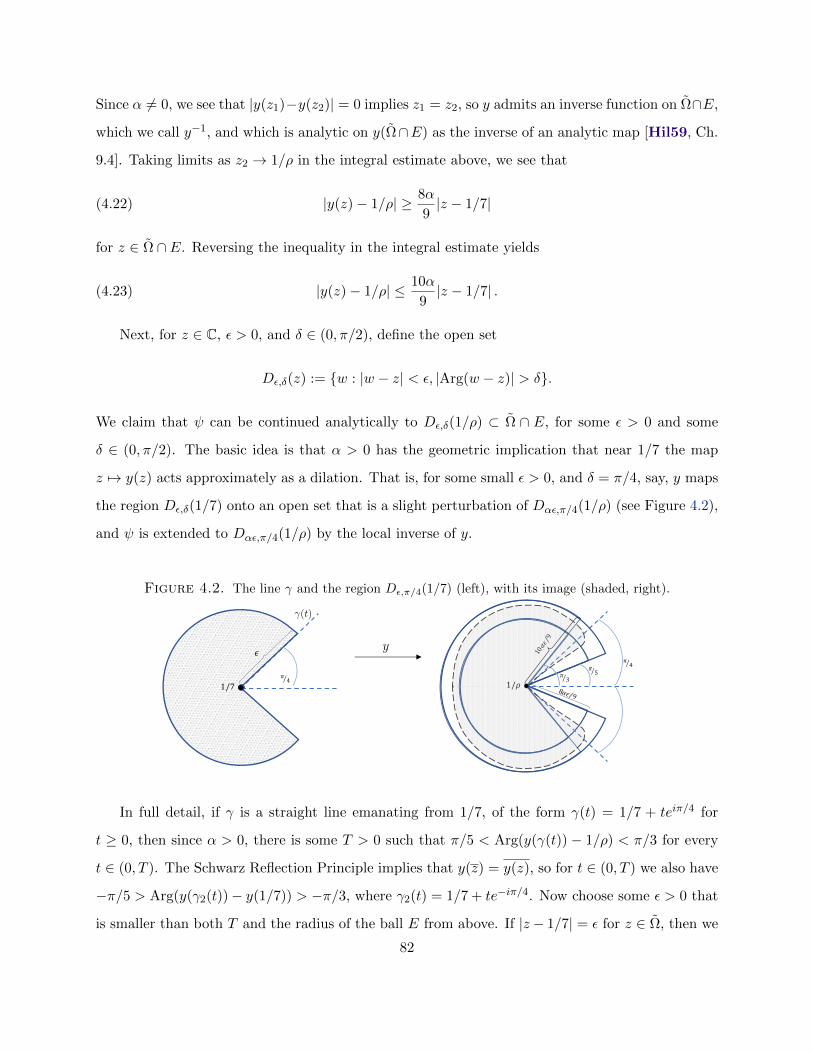
Since α 6= 0, we see that |y(z1)−y(z2)| = 0 implies z1 = z2, so y admits an inverse function on Ω∩E,
which we call y−1, and which is analytic on y(Ω∩E) as the inverse of an analytic map [Hil59, Ch.
9.4]. Taking limits as z2 → 1/ρ in the integral estimate above, we see that
(4.22) |y(z)− 1/ρ| ≥ 8α
9|z − 1/7|
for z ∈ Ω ∩ E. Reversing the inequality in the integral estimate yields
(4.23) |y(z)− 1/ρ| ≤ 10α
9|z − 1/7| .
Next, for z ∈ C, ε > 0, and δ ∈ (0, π/2), define the open set
Dε,δ(z) := w : |w − z| < ε, |Arg(w − z)| > δ.
We claim that ψ can be continued analytically to Dε,δ(1/ρ) ⊂ Ω ∩ E, for some ε > 0 and some
δ ∈ (0, π/2). The basic idea is that α > 0 has the geometric implication that near 1/7 the map
z 7→ y(z) acts approximately as a dilation. That is, for some small ε > 0, and δ = π/4, say, y maps
the region Dε,δ(1/7) onto an open set that is a slight perturbation of Dαε,π/4(1/ρ) (see Figure 4.2),
and ψ is extended to Dαε,π/4(1/ρ) by the local inverse of y.
Figure 4.2. The line γ and the region Dε,π/4(1/7) (left), with its image (shaded, right).
γ(t)
𝜋4#
1/7
𝜖
8𝛼𝜖/9
𝜋3#
𝜋5#
𝜋4#
1/𝜌
10𝛼𝜖/9
y
In full detail, if γ is a straight line emanating from 1/7, of the form γ(t) = 1/7 + teiπ/4 for
t ≥ 0, then since α > 0, there is some T > 0 such that π/5 < Arg(y(γ(t)) − 1/ρ) < π/3 for every
t ∈ (0, T ). The Schwarz Reflection Principle implies that y(z) = y(z), so for t ∈ (0, T ) we also have
−π/5 > Arg(y(γ2(t))− y(1/7)) > −π/3, where γ2(t) = 1/7 + te−iπ/4. Now choose some ε > 0 that
is smaller than both T and the radius of the ball E from above. If |z− 1/7| = ε for z ∈ Ω, then we
82

have from estimates (4.22) and (4.23) that
8αε
9≤ |y(z)− 1/ρ| ≤ 10αε
9.
Thus, we have described the images of the two line segments and the circular arc that make up
the boundary of Dε,π/4, and our description implies that the image of Dε,π/4(1/7) contains the open
set D8αε/9,π/3(1/ρ), as shown in Figure 4.2. We also saw above that y−1 is analytic on y(Ω ∩ E)
and hence on D8αε/9,π/3(1/ρ), which intersects Λ in a nonempty open set. Thus, if we redefine ε to
denote the value 8αε/9 from above, and also set δ = π/3, then y−1 extends ψ to Dε,δ(1/ρ), as was
to be shown. By construction we have the inverse relationship (y ψ)|Dε,δ(1/ρ) = Id |Dε,δ(1/ρ).
To finish extending ψ to ∆1/ρ, it suffices by compactness of the set ∂Λ \ Dε,δ(1/ρ) to obtain
analytic continuations of ψ around all points in an arbitrary finite subcollection of ∂Λ \ 1/ρ.
Let w ∈ ∂Λ \ 1/ρ. The two supporting claims in the proof of Lemma 4.3.4 imply that
ψ(w) ∈ Ω. We claim that y′(ψ(w)) 6= 0. To see why this is true, let γ be the straight line path
from 0 to w. If 0 = y′(ψ(w)), then recalling from Lemma 4.3.4 that y ψ = Id |Λ we see that
y(ψ(w)) = w for w ∈ γ. Therefore,
0 = limw→w,w∈γ
|y′(ψ(w))| = limw→w,w∈γ
1/|ψ′(w)|,
which implies that |ψ′(w)| → ∞ as w → w along γ. This contradicts the fact from Lemma 4.3.3
that ψ′ extends continuously to ∂Λ and so is bounded there. So y′(ψ(w)) 6= 0. By the inverse
function theorem, y is locally invertible at ψ(w), and the local inverse extends ψ analytically to a
neighborhood of w that maps into Ω.
We have extended ψ to a Delta-domain ∆1/ρ by patching together local inverses of y. To see
that y is a global inverse of ψ, one need only observe that ψ(∆1/ρ) ⊂ Ω, by construction. It follows
that y is analytic on ψ(∆1/ρ), and (y ψ)|∆1/ρ= Id |∆1/ρ
by the principle of permanence.
4.3.4. Asymptotic singular expansion of ψ near y(1/7). Let ∆1/ρ be the Delta-domain
from Proposition 4.3.3. We apply a “bootstrapping” procedure to (4.8) that locally inverts y near
1/7, up to an asymptotically negligible error term, resulting in an asymptotic singular expansion
for ψ = y−1 near the singularity 1/ρ (the general idea of bootstrapping and some examples are
discussed in [DB58, Ch. 2]). Precisely, we show the following, with λ as in (4.19).
83
Proposition 4.3.4. Set V = 1− ρz. The function ψ admits the following singular expansion:
as z → 1/ρ in ∆1/ρ,
(4.24) ψ(z) = γ(V ) + CV 6 log V +O(V 7 log V ),
where
C =75Kρ
6!(7 + ρλ)7,
and γ is a degree-six polynomial with γ(0) = 1/7. Furthermore, the error term ψ(z) − γ(V ) −
CV 6 log V is analytic in ∆1/ρ.
Before the proof we illustrate the bootstrapping technique with a small example, which could
also be skipped.
Example 4.3.1. Consider the equation z = w + w2 + w2 logw. Then w ∼ z, as w, z → 0, and
log z = logw+ log(1 +w+w logw) = logw+O(w logw). It follows that logw = log z+O(z log z).
Since w = z − w2 + w2 logw, we therefore have w2 = z2 + O(z3 log z). Plugging back into the
original equation, this yields
w = z − z2 − z2 log z +O(z3 log z).
The proof of the proposition is similar, but more involved.
Proof of Proposition 4.3.4. With Z = 1− 7z, (4.8) implies that
y(z) =1− Z
7
(p(Z)− K
6!Z6 logZ +O(Z7 logZ)
),
as z → 1/7 ∈ Ω. By the identity (y ψ)|∆1/ρ= Id |∆1/ρ
, if we evaluate both sides of the equation
at ψ(z), for z in a small neighborhood of 1/ρ in ∆1/ρ, and if we apply the change of variables
Y = 1− 7ψ(z), then we obtain
1− Z7
= z = y(ψ(z)) =1− Y
7
(p(Y )− K
6!Y 6 log(Y ) +O(Y 7 log Y )
),
which implies
(4.25) Z − 1 = (Y − 1)
(p(Y )− K
6!Y 6 log Y +O(Y 7 log Y )
),
84

as z → 1/ρ in ∆1/ρ. In (4.15) we see that p(Y ) = (−K/6!) log(21/8)Y 6 +∑6
n=0 fnYn. Thus, upon
setting
W =Z + f0 − 1
f0 − f1,
we find from (4.25) that as z → 1/ρ in ∆1/ρ,
(4.26) Y = W − (Q(Y ) + cY 6 log Y +O(Y 7 log Y )),
where
Q(Y ) =f1 − f2f0 − f1
Y 2 +f2 − f3f0 − f1
Y 3 +f3 − f4f0 − f1
Y 4 +f4 − f5f0 − f1
Y 5 +f5 − f6 + K
6! log(218
)f0 − f1
Y 6,
and
c =K
6!(f0 − f1)=
K
6!(7/ρ+ λ).
For simpler notation, define the list of constants (ai)6i=2 ⊂ R so that Q(Y ) =
∑6i=2 aiY
i.
W (z) and Y (z) tend to 0 as z → 1/ρ in ∆1/ρ. It follows then from (4.26) that W ∼ Y as
z → 1/ρ. Therefore, Y = O(W ) and log(Y ) ∼ log(W ) (as z → 1/ρ in ∆1/ρ, which is assumed for
the rest of the proof). These estimates for Y imply that
Q(Y ) = a2W2 +O(W 3) ,
which, upon substitution into (4.26), yields
Y = W − a2W2 +O(W 3).
We substitute this new estimate for Y into Q(Y ), which yields
Q(Y ) = a2W2 + (a3 − 2a2
2)W 3 +O(W 4),
and hence, from (4.26),
Y = W − a2W2 − (a3 − 2a2
2)W 3 +O(W 4).
85

After another iteration, we obtain from (4.26) that
Y = W −Q(Y ) +O(W 5)
= W − a2W2 − (a3 − 2a2
2)W 3 − (5a32 − 5a2a3 + a4W
4) +O(W 5).
After a final iteration, we obtain from (4.26) that
Y = W − a2W2 − · · · − a′6W 6 +O(W 7) + cY 6 log Y +O(Y 7 log Y ),
where a′6 is an unimportant constant. Since Y = W +O(W 2), we have that the O(Y 7 log Y ) error
term is O(W 7 logW ), and that Y 6 log Y = W 6 logW +O(W 7 logW ). We can therefore express Y
in terms of W as follows:
Y = W − a2W2 − · · · − a′6W 6 + cW 6 logW +O(W 7 logW ) .
We substitute ψ(z) = (1− Y )/7 in the latter expression, obtaining
(4.27) ψ(z) =1
7+ P (W ) +
c
7W 6 log(W ) +O(W 7 logW ),
with P (0) = 0.
To finish the proof, it just remains to write W in terms of V :
W =Z + f0 − 1
f0 − f1=Z + 7/ρ− 1
7/ρ+ λ=
7/ρ− 7z
7/ρ+ λ=
7
7 + ρλ(1− ρz) =
7
7 + ρλV .
Substituting the last expression into (4.27) leads immediately to (4.24), with
γ(V ) =1
7+ P
(7
7 + ρλV
),
and
C =c
7
(7
7 + ρλ
)6
=75Kρ
6!(7 + ρλ)7.
The error term in (4.27) is analytic in ∆1/ρ since all the other terms are.
4.3.5. Asymptotic singular expansion of A near y(1/7). Since ψ is injective on ∆1/ρ by
Proposition 4.3.3, and ψ(0) = 0, we see that A(z) = z/ψ(z) extends to be analytic on ∆1/ρ. We
seek its singular expansion near 1/ρ = y(1/7). Let C be the constant from Proposition 4.3.4.
86
Proposition 4.3.5. Set V = 1− ρz. The function A admits the following singular expansion:
as z → 1/ρ in ∆1/ρ,
(4.28) A(z) = η(V )− 49C
ρV 6 log V +O(V 7 log V ),
where η is a degree-seven polynomial. The error term A(z) + (49C/ρ)V 6 log V − η(V ) is analytic
in ∆1/ρ.
Proof. Referring to Proposition 4.3.4, let E(V ) denote the error term in (4.24), namely,
E(V ) = ψ(z)− γ(V )− CV 6 log V.
E(V ) is visibly analytic on ∆1/ρ. Let (bi)6i=0 ⊂ R be such that γ(V ) =
∑6i=0 biV
6 (e.g. b0 = 1/7).
Define the polynomial
T (V ) = −49(49b32 − 7b23 − 14b2b4 + b6
)V 6 + 49 (14b2b3 − b5)V 5(4.29)
+ 49(7b22 − b4
)V 4 − 49b3V
3 − 49b2V2 + 7 .
Also define S(V ) = T (V )− 49CV 6 log V , which is analytic on ∆1/ρ.
A routine computation shows that
ψ(z)S(V ) =
[(1
7+
6∑i=1
biVi
)+ CV 6 log V + E(V )
] [T (V )− 49CE(V )V 6 log V
]= 1 + E(V )T (V )− 49CE(V )V 6 log(V ) +
[12∑i=7
V i · di(log V )
],
where di(x) is a linear polynomial, for 7 ≤ i ≤ 11, and d12(x) is a quadratic polynomial. It follows
that
E(V ) := ψ(z)S(V )− 1
is analytic on ∆1/ρ and O(V 7 log V ) as z → 1/ρ in ∆1/ρ. We write this as
1
ψ(z)= S(V )− E(V )
ψ(z),
87

or, since z = (1− V )/ρ,
A(z) =z
ψ(z)=
(1− V )
ρS(V )−A(z)E(V ).
Comparing the latter equation with (4.29), we see that
A(z) = −49C
ρV 6 log(V ) + η(V ) + ˜E(V ) ,
where
η(V ) =1− Vρ
(S(V ) + 49CV 6 log V )
is a degree-seven polynomial, and the error term
˜E(V ) :=49C
ρV 7 log(V )−A(z) ˜E(V )
is analytic in ∆1/ρ and O(V 7 log V ) as z → 1/ρ.
4.3.6. Asymptotic formula for (an). By (4.16), (4.28), and Theorem 1.4.4, we have
an =49 · C · 6!
ρ· 7n
(1
n7+O
(log n
n8
)),
as n→∞. Since 49 ·C ·6! is precisely the constant M from (1.18), this verifies (1.23) and completes
the proof of Theorem 1.4.1.
4.4. The case of the Lie algebra B2
In this final section of the chapter we consider the analogous sharpness question from Kuper-
berg’s conjecture for the Lie algebra B2, which is a rank-2 Lie algebra of dimension 10. We will
follow the discussion on OEIS [SI20] for the sequences indexed by A005700 and A194091. Although
our presentation will be somewhat informal, we hope to indicate how some of the preceding ideas
can be used in other situations.
We define the sequence (dn)∞n=0 analogously to (bn)∞n=0, except that we modify for the fact
that dim InvB2(V (λ1)⊗n) = 0 when n is odd, where λ1 is the fundamental weight for B2 with a
4-dimensional representation. Thus d0 := 1, and for n ≥ 1 we define (OEIS: A005700)
dn = dim InvB2(V (λ1)⊗2n) .
88
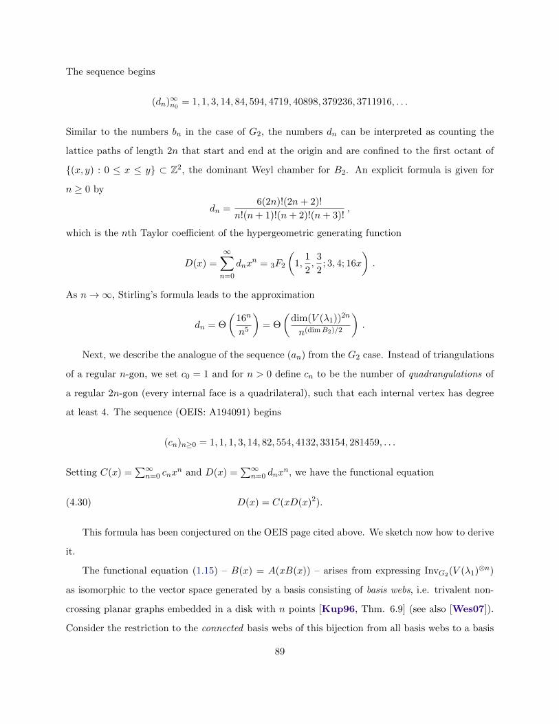
The sequence begins
(dn)∞n0= 1, 1, 3, 14, 84, 594, 4719, 40898, 379236, 3711916, . . .
Similar to the numbers bn in the case of G2, the numbers dn can be interpreted as counting the
lattice paths of length 2n that start and end at the origin and are confined to the first octant of
(x, y) : 0 ≤ x ≤ y ⊂ Z2, the dominant Weyl chamber for B2. An explicit formula is given for
n ≥ 0 by
dn =6(2n)!(2n+ 2)!
n!(n+ 1)!(n+ 2)!(n+ 3)!,
which is the nth Taylor coefficient of the hypergeometric generating function
D(x) =
∞∑n=0
dnxn = 3F2
(1,
1
2,3
2; 3, 4; 16x
).
As n→∞, Stirling’s formula leads to the approximation
dn = Θ
(16n
n5
)= Θ
(dim(V (λ1))2n
n(dimB2)/2
).
Next, we describe the analogue of the sequence (an) from the G2 case. Instead of triangulations
of a regular n-gon, we set c0 = 1 and for n > 0 define cn to be the number of quadrangulations of
a regular 2n-gon (every internal face is a quadrilateral), such that each internal vertex has degree
at least 4. The sequence (OEIS: A194091) begins
(cn)n≥0 = 1, 1, 1, 3, 14, 82, 554, 4132, 33154, 281459, . . .
Setting C(x) =∑∞
n=0 cnxn and D(x) =
∑∞n=0 dnx
n, we have the functional equation
(4.30) D(x) = C(xD(x)2).
This formula has been conjectured on the OEIS page cited above. We sketch now how to derive
it.
The functional equation (1.15) – B(x) = A(xB(x)) – arises from expressing InvG2(V (λ1)⊗n)
as isomorphic to the vector space generated by a basis consisting of basis webs, i.e. trivalent non-
crossing planar graphs embedded in a disk with n points [Kup96, Thm. 6.9] (see also [Wes07]).
Consider the restriction to the connected basis webs of this bijection from all basis webs to a basis
89
of InvG2(V (λ1)⊗n). These connected basis webs correspond to the triangulations counted by (an),
as explained after Theorem 8.1 in [Kup96] (essentially by the definition of “non-elliptic” – in the
terminology of the paper – and the fact that trivalent vertices can be used to generate all basis webs
for this representation, as well as the duality between triangulations and connected basis webs).
Then (1.15) follows from organizing the connected components of a basis web into a rooted planar
tree in a particular way.
In the case of B2, the construction is isomorphic, except that the basis webs are generated by
a tetravalent vertex (as opposed to trivalent). This and the non-elliptic condition translate – upon
passing to dual graphs – respectively to the properties of having each face in the cover of an n-gon
be a square (not a triangle) and having each internal vertex possess no fewer than 4 (not 6) edges.
What we obtain then is that
(4.31) D(x) = C(xD(x)) ,
where C(x) =∑
n≥0 cnxn and D(x) =
∑n≥0 dnx
n with cn the number of quadrangulations of an
n-gon and dn = dim InvB2(V (λ1)n). Since cn = dn = 0 when n is odd, we can write C(x2) = C(x)
and D(x2) = D(x) to obtain (4.30).
Theorems 1.4.2 and 4.1.2 do not directly apply to (4.31), since the gcd condition is not met
for the generating function C(x), which is even. However, in the paragraph after Theorem 4.1.2 it
is stated that the gcd condition is a mild technically. Indeed, as the reader would see in pursuing
the references indicated there, our sharpness conclusion still follows in (4.31) by considering sub-
sequences, i.e. from the fact that the sequence (dn)n≥0 is supported on the even positive integers
and that d2n/16n 6= Θ(n−3/2) as n → ∞. Or, an alternative argument is obtained by applying
the reasoning in Remark 4.1.3 to the subsequence (d2n)n≥0. In any case, one finds that the radius
of convergence of C(x) is precisely D(1/4)/4, which implies that C(x) has radius of convergence
D(1/16)2/16. In other words, we have the following result:
Theorem 4.4.1.
lim supn→∞
n√cn =
16
D(1/16)2=
16
3F2
(1, 1
2 ,32 ; 3, 4; 1
)2 =225π2
4(165π − 512)2,
with an approximate value of 13.7128.
90

Applying Fekete’s lemma as we did for (an) we can easily pass to the limit. Also, since D(x)
is given explicitly here, one could potentially use appropriate expansions of 3F2 to give an al-
ternative proof of asymptotic sharpness by an inverse function theorem argument, like we did in
Section 4.3.2.4. With more motivation one might even deduce a true asymptotic formula by a
bootstrapping procedure, as we did for (an).
91
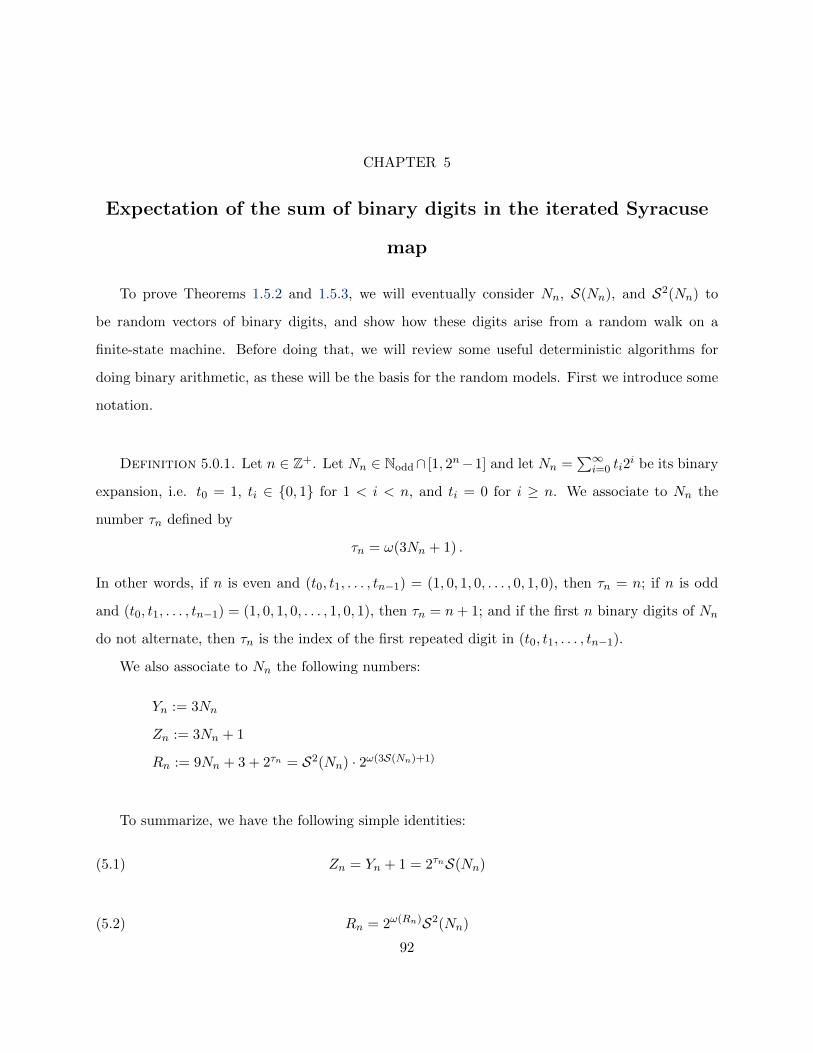
CHAPTER 5
Expectation of the sum of binary digits in the iterated Syracuse
map
To prove Theorems 1.5.2 and 1.5.3, we will eventually consider Nn, S(Nn), and S2(Nn) to
be random vectors of binary digits, and show how these digits arise from a random walk on a
finite-state machine. Before doing that, we will review some useful deterministic algorithms for
doing binary arithmetic, as these will be the basis for the random models. First we introduce some
notation.
Definition 5.0.1. Let n ∈ Z+. Let Nn ∈ Nodd∩ [1, 2n−1] and let Nn =∑∞
i=0 ti2i be its binary
expansion, i.e. t0 = 1, ti ∈ 0, 1 for 1 < i < n, and ti = 0 for i ≥ n. We associate to Nn the
number τn defined by
τn = ω(3Nn + 1) .
In other words, if n is even and (t0, t1, . . . , tn−1) = (1, 0, 1, 0, . . . , 0, 1, 0), then τn = n; if n is odd
and (t0, t1, . . . , tn−1) = (1, 0, 1, 0, . . . , 1, 0, 1), then τn = n+ 1; and if the first n binary digits of Nn
do not alternate, then τn is the index of the first repeated digit in (t0, t1, . . . , tn−1).
We also associate to Nn the following numbers:
Yn := 3Nn
Zn := 3Nn + 1
Rn := 9Nn + 3 + 2τn = S2(Nn) · 2ω(3S(Nn)+1)
To summarize, we have the following simple identities:
(5.1) Zn = Yn + 1 = 2τnS(Nn)
(5.2) Rn = 2ω(Rn)S2(Nn)
92
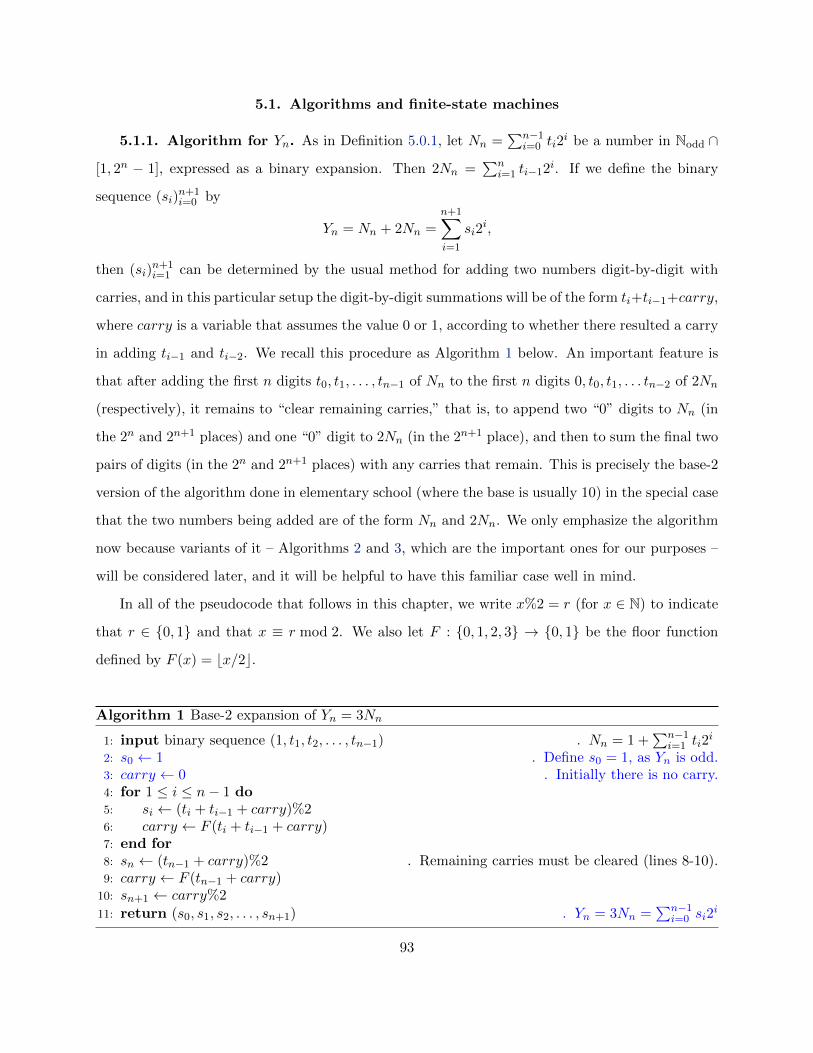
5.1. Algorithms and finite-state machines
5.1.1. Algorithm for Yn. As in Definition 5.0.1, let Nn =∑n−1
i=0 ti2i be a number in Nodd ∩
[1, 2n − 1], expressed as a binary expansion. Then 2Nn =∑n
i=1 ti−12i. If we define the binary
sequence (si)n+1i=0 by
Yn = Nn + 2Nn =n+1∑i=1
si2i,
then (si)n+1i=1 can be determined by the usual method for adding two numbers digit-by-digit with
carries, and in this particular setup the digit-by-digit summations will be of the form ti+ti−1+carry,
where carry is a variable that assumes the value 0 or 1, according to whether there resulted a carry
in adding ti−1 and ti−2. We recall this procedure as Algorithm 1 below. An important feature is
that after adding the first n digits t0, t1, . . . , tn−1 of Nn to the first n digits 0, t0, t1, . . . tn−2 of 2Nn
(respectively), it remains to “clear remaining carries,” that is, to append two “0” digits to Nn (in
the 2n and 2n+1 places) and one “0” digit to 2Nn (in the 2n+1 place), and then to sum the final two
pairs of digits (in the 2n and 2n+1 places) with any carries that remain. This is precisely the base-2
version of the algorithm done in elementary school (where the base is usually 10) in the special case
that the two numbers being added are of the form Nn and 2Nn. We only emphasize the algorithm
now because variants of it – Algorithms 2 and 3, which are the important ones for our purposes –
will be considered later, and it will be helpful to have this familiar case well in mind.
In all of the pseudocode that follows in this chapter, we write x%2 = r (for x ∈ N) to indicate
that r ∈ 0, 1 and that x ≡ r mod 2. We also let F : 0, 1, 2, 3 → 0, 1 be the floor function
defined by F (x) = bx/2c.
Algorithm 1 Base-2 expansion of Yn = 3Nn
1: input binary sequence (1, t1, t2, . . . , tn−1) . Nn = 1 +∑n−1
i=1 ti2i
2: s0 ← 1 . Define s0 = 1, as Yn is odd.3: carry ← 0 . Initially there is no carry.4: for 1 ≤ i ≤ n− 1 do5: si ← (ti + ti−1 + carry)%26: carry ← F (ti + ti−1 + carry)7: end for8: sn ← (tn−1 + carry)%2 . Remaining carries must be cleared (lines 8-10).9: carry ← F (tn−1 + carry)
10: sn+1 ← carry%211: return (s0, s1, s2, . . . , sn+1) . Yn = 3Nn =
∑n−1i=0 si2
i
93

Algorithm 1 can be described as a (n+ 1)-step walk on the directed graph shown in Figure 5.1,
which has four nodes or states. Let us explain the connection. Initially a walker starts at state A.
The pair 1/N labelling the node A is meant to indicate that t0 = 1 and that no carry is present at
the start of the algorithm (“N” for “no carry” – not to be confused with the natural number Nn).
The walker’s first step depends on t1, in the following way. If t1 = 0, then the walker moves along
the edge labelled 0/1 to node B. The “0” in the label is the value of t1, and the “1” in the label is
the value of s1 in the Algorithm 1 for Yn. Notice that in state B the pair 0/N indicates that t1 = 0
and that no carry resulted in adding t0 and t1 to obtain s1. If, on the other hand, t1 = 1, then the
walker would move from state A along the edge labelled 1/0. The “1” is the value of t1, and the
“0” is the value of s1. In this case a carry results from adding t0 and t1, and accordingly state C
is labelled with 1/Y to indicate that t1 = 1 and that “yes” a carry resulted.
A: 1/N B: 0/N
C: 1/Y D: 0/Y
0/1
1/1
1/0
0/0
0/1
1/0
0/01/1
Figure 5.1. 4-state machine representing Nn 7→ Yn = 3Nn and Nn 7→ Zn = 3Nn + 1.
So far we have only described the initial step a walker takes and the relationship of this step to
t1 and s1 as well as the meaning of the labels. But the walker will take n+ 1 steps in total, and the
ith step in general corresponds to the declaration of si in Algorithm 1. Let us explain this further.
Generalizing the labeling scheme above for t1 and s1 to ti and si with i > 1, we will interpret labels
above edges as input/output pairs, with the input being ti and the output being si; and we will
interpret the label of the ith state as indicating the value of ti and the current value of the variable
94
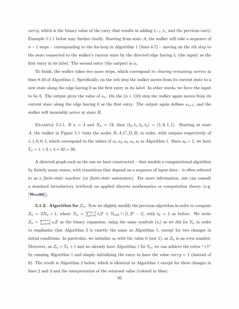
carry, which is the binary value of the carry that results in adding ti−1, ti, and the previous carry.
Example 5.1.1 below may further clarify. Starting from state A, the walker will take a sequence of
n− 1 steps – corresponding to the for-loop in Algorithm 1 (lines 4-7) – moving on the ith step to
the state connected to the walker’s current state by the directed edge having ti (the input) as the
first entry in its label. The second entry (the output) is si.
To finish, the walker takes two more steps, which correspond to clearing remaining carries in
lines 8-10 of Algorithm 1. Specifically, on the nth step the walker moves from its current state to a
new state along the edge having 0 as the first entry in its label. In other words, we force the input
to be 0. The output gives the value of sn. On the (n+ 1)th step the walker again moves from its
current state along the edge having 0 as the first entry. The output again defines sn+1, and the
walker will invariably arrive at state B.
Example 5.1.1. If n = 4 and Nn = 13, then (t0, t1, t2, t3) = (1, 0, 1, 1). Starting at state
A, the walker in Figure 5.1 visits the nodes B,A,C,D,B, in order, with outputs respectively of
1, 1, 0, 0, 1, which correspond to the values of s1, s2, s3, s4, s5 in Algorithm 1. Since s0 = 1, we have
Yn = 1 + 2 + 4 + 32 = 39.
A directed graph such as the one we have constructed – that models a computational algorithm
by finitely many states, with transitions that depend on a sequence of input data – is often referred
to as a finite-state machine (or finite-state automaton). For more information, one can consult
a standard introductory textbook on applied discrete mathematics or computation theory (e.g.
[Woo86]).
5.1.2. Algorithm for Zn. Now we slightly modify the previous algorithm in order to compute
Zn = 3Nn + 1, where Nn =∑n−1
i=0 ti2i ∈ Nodd ∩ [1, 2n − 1], with t0 = 1 as before. We write
Zn =∑n+1
s=0 si2i as the binary expansion, using the same symbols (si) as we did for Yn in order
to emphasize that Algorithm 2 is exactly the same as Algorithm 1, except for two changes in
initial conditions. In particular, we initialize s0 with the value 0 (not 1), as Zn is an even number.
Moreover, as Zn = Yn + 1 and we already have Algorithm 1 for Yn, we can achieve the extra “+1”
by running Algorithm 1 and simply initializing the carry to have the value carry = 1 (instead of
0). The result is Algorithm 2 below, which is identical to Algorithm 1 except for these changes in
lines 2 and 3 and the interpretation of the returned value (colored in blue).
95

Algorithm 2 Base-2 expansion of Zn = 3Nn + 1
1: input binary sequence (1, t1, t2, . . . , tn−1) . Nn = 1 +∑n−1
i=1 ti2i
2: s0 ← 0 . Define s0 = 0, as Zn is odd.3: carry ← 1 . Initialize the carry as 1.4: for 1 ≤ i ≤ n− 1 do5: si ← (ti + ti−1 + carry)%26: carry ← F (ti + ti−1 + carry)7: end for8: sn ← (tn−1 + carry)%2 . Remaining carries must be cleared (lines 8-10).9: carry ← F (tn−1 + carry)
10: sn+1 ← carry%211: return (s0, s1, s2, . . . , sn+1) . Zn = 3Nn + 1=
∑n−1i=0 si2
i
In terms of the finite-state machine in Figure 5.1, the change of initial conditions that differ-
entiates Algorithm 2 from Algorithm 1 translates to the walker for this model of Zn beginning its
journey in state C, not in state A as before. The rest of the walk proceeds with the same rules,
including for the last two steps, for which the input is 0 (clearing remaining carries). The walker
invariably ends in state B, as before.
Example 5.1.2. If n = 5 and Nn = 19, then (t0, t1, t2, t3, t4) = (1, 1, 0, 0, 1). Starting at state
C the walker in Figure 5.1 visits the nodes C,D,B,B,A,B,B, in order, with outputs respectively
of 1, 0, 1, 1, 1, 0 which correspond to the values of s1, s2, s3, s4, s5, s6 in Algorithm 2. Since s0 = 0,
we have Zn = 2 + 8 + 16 + 32 = 58.
5.1.3. Algorithm for Rn. The 4-state machine introduced above was a model for algorithms
that compute the values Yn = 3Nn and Zn = 3Nn + 1, or, more precisely, their sequences of binary
digits. Each digit ti of Nn acts as an input that results in the ith step of the machine or algorithm.
In this section we present Algorithm 3 (below) and an associated 16-state machine, which produce
the analogous sequence of outputs in the operation Nn 7→ Rn = 9Nn + 3 + 2τn . That is, the
algorithm produces the vector of binary digits (r0, r1, . . . , rn+3) of Rn =∑n+3
i=1 ri2i.
To introduce the procedure, let us suggest that in ignoring all references to the sequence (ri)n+3i=0
in the psuedocode of Algorithm 3, the reader will see that Algorithm 3 reduces to Algorithm 2 for
the sequence (si)n+1i=0 of binary digits in Zn in the specific case that Zn is not a power of 2 (which
is precisely the case in which the if-condition is false in lines 2-3 of Algorithm 3). In particular,
as i ranges over 1, 2, . . . , τn in the for-loop in lines 5-8 of Algorithm 3, the same values of si are
produced as are produced as i ranges over the same set in the for-loop in lines 4-7 of Algorithm 2,
96

namely si ≡ 0. Then, as i ranges over τn, τn + 1, . . . , n − 1 in lines 13-18 of Algorithm 3, the
same values of si are produced as are produced when i ranges over the same set in lines 5-8 of
Algorithm 2; and moreover, the exact same procedure involving carries is used in both cases. After
that, the clearing of the carries is done exactly the same way in both algorithms, with carry1 in
Algorithm 3 playing the role that carry played in Algorithm 2. One might therefore argue that
with respect to the sequence (si)n+1i=0 , the only difference between the two algorithms is in how
they produce the initial string of τn “0”s in the sequence of binary digits of Zn. In some sense
then, Algorithm 2 is redundant. But it seems reasonable to isolate the computation of Zn, as we
will specifically rely on it later, and to also gradually lead the reader into an understanding of
Algorithm 3 Base-2 expansion of Rn = 9Nn + 3 + 2τn
1: input binary sequence (1, t1, t2, . . . , tn−1) . Nn = 1 +∑n−1
i=1 ti2i
2: if τn ≥ n or ti = 0 for i ≥ τn then
3: return (
τn+1 times︷ ︸︸ ︷0, 0, . . . , 0, 1) . 9Nn + 3 + 2τn = 2τn+2
4: end if5: for 0 ≤ i < τn do6: si ← 07: ri ← 08: end for9: sτn ← 1
10: rτn ← 011: carry1 ← τn%212: carry2 ← 113: for τn < i ≤ n− 1 do14: si ← (ti + ti−1 + carry1)%215: carry1 ← F (ti + ti−1 + carry1)16: ri ← (si + si−1 + carry2)%217: carry2 ← F (si + si−1 + carry2)18: end for19: sn ← (tn−1 + carry1)%2 . Lines 19-28 are clearing the carries.20: carry1 ← F (tn−1 + carry1)21: rn ← (sn + sn−1 + carry2)%222: carry2 ← F (sn + sn−1 + carry2)23: sn+1 ← carry1%224: rn+1 ← (sn+1 + sn + carry2)%225: carry2 ← F (sn+1 + sn + carry2)26: rn+2 ← (sn+1 + carry2)%227: carry2 ← F (sn+1 + carry2)28: rn+3 ← carry2%229: return (r0, r1, r2, . . . , rn+3) . Rn =
∑r+3i=0 ri2
i
97

Algorithm 3, which at first glance might appear to be much more involved than the previous two,
but is actually quite natural.
Computationally, the upshot of Algorithm 3 regards the sequence (ri)n+3i=0 . Indeed, for 1 ≤ i ≤
n+ 1, the value ri is produced in the algorithm as soon as si is produced (i.e. in the same step of
a for-loop or in the formal sense that ri is a function of si, si−1, and the two carries involved, as
we explain in more detail below). Therefore ri is known as soon as tk : k ≤ i is known. This will
be useful later when we consider ri – as a random variable – to be a deterministic function of the
random binary vector (t0, t1, . . . , ti).
The reader is invited to work through the pseudocode, or to use the SAGE implementation
provided in Figure 5.3. We explain the recursive mechanism at work. The key observation from
arithmetic is that if Nn =∑∞
i=0 ti2i is an odd number written in binary, then in order to determine
the binary digit sk in the expansion Zn = 3Nn+ 1 =∑∞
i=0 si2i, it is sufficient to know tk, tk−1, and
whether a carry resulted when adding tk−1, tk−2, and any inherited carry from prior steps. Indeed
this is the underlying idea for the 4-state model. Similarly, in the expansion Rn = 3Zn + 2τn =∑∞i=0 ri2
i , we see that rk can determined if we know sk, sk−1, and whether a carry resulted from
adding sk−1 and sk−2. Thus, the following four data points determine the value of rk, given the
input tk:
(1) tk−1
(2) binary value of carry resulting from tk−1 + tk−2 (+ any inherited carry)
(3) sk−1
(4) binary value of carry resulting from sk−1 + sk−2 (+ any inherited carry)
Furthermore, upon receiving the input tk, one can obviously determine from the latter quadruple
of information – which we refer to as the (k− 1)th state – the subsequent quadruple of information
– which defines the kth state – namely:
(1) tk(2) binary value of carry resulting from tk + tk−1 (+ any inherited carry)
(3) sk(4) binary value of carry resulting from sk + sk−1 (+ any inherited carry)
Thus, each such quadruple of information can be viewed as a a node in a directed graph
from which we pass to another node upon knowing a new digit in the sequence (ti). Algorithm 3
formalizes this process, with carry1 and carry2 keeping track of the carries involved in adding values
98
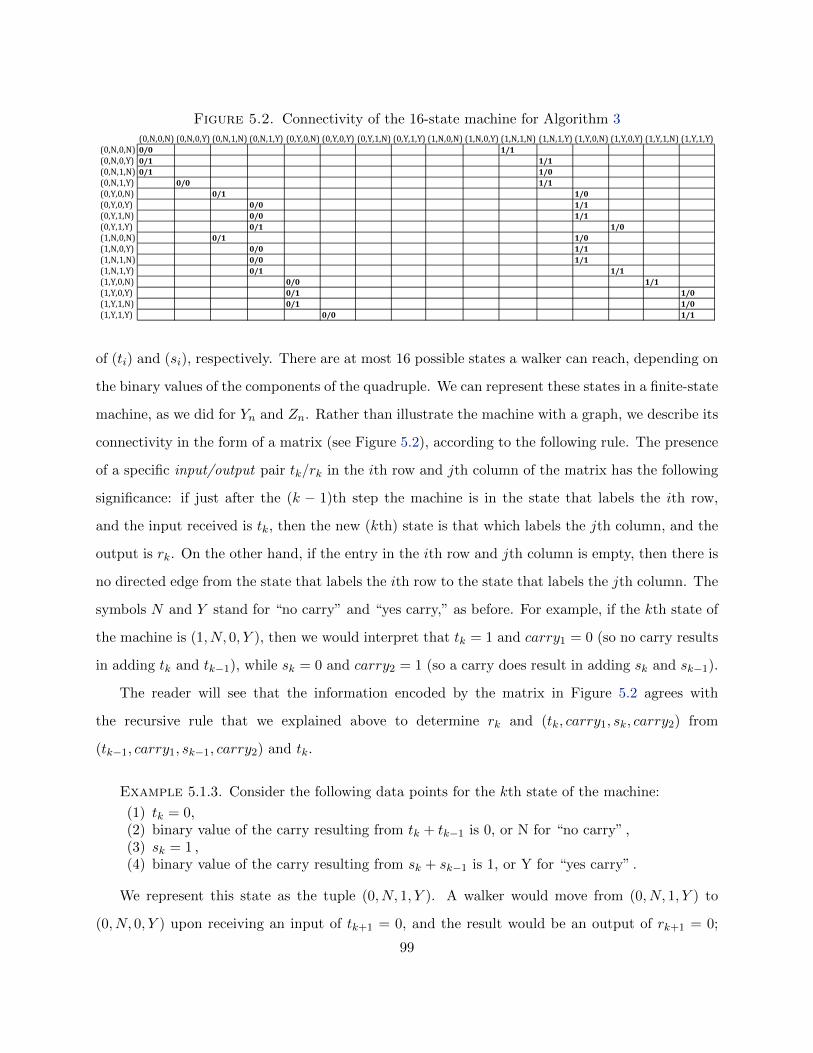
Figure 5.2. Connectivity of the 16-state machine for Algorithm 3
(0,N,0,N) (0,N,0,Y) (0,N,1,N) (0,N,1,Y) (0,Y,0,N) (0,Y,0,Y) (0,Y,1,N) (0,Y,1,Y) (1,N,0,N) (1,N,0,Y) (1,N,1,N) (1,N,1,Y) (1,Y,0,N) (1,Y,0,Y) (1,Y,1,N) (1,Y,1,Y)(0,N,0,N) 0/0 1/1(0,N,0,Y) 0/1 1/1(0,N,1,N) 0/1 1/0(0,N,1,Y) 0/0 1/1(0,Y,0,N) 0/1 1/0(0,Y,0,Y) 0/0 1/1(0,Y,1,N) 0/0 1/1(0,Y,1,Y) 0/1 1/0(1,N,0,N) 0/1 1/0(1,N,0,Y) 0/0 1/1(1,N,1,N) 0/0 1/1(1,N,1,Y) 0/1 1/1(1,Y,0,N) 0/0 1/1(1,Y,0,Y) 0/1 1/0(1,Y,1,N) 0/1 1/0(1,Y,1,Y) 0/0 1/1
of (ti) and (si), respectively. There are at most 16 possible states a walker can reach, depending on
the binary values of the components of the quadruple. We can represent these states in a finite-state
machine, as we did for Yn and Zn. Rather than illustrate the machine with a graph, we describe its
connectivity in the form of a matrix (see Figure 5.2), according to the following rule. The presence
of a specific input/output pair tk/rk in the ith row and jth column of the matrix has the following
significance: if just after the (k − 1)th step the machine is in the state that labels the ith row,
and the input received is tk, then the new (kth) state is that which labels the jth column, and the
output is rk. On the other hand, if the entry in the ith row and jth column is empty, then there is
no directed edge from the state that labels the ith row to the state that labels the jth column. The
symbols N and Y stand for “no carry” and “yes carry,” as before. For example, if the kth state of
the machine is (1, N, 0, Y ), then we would interpret that tk = 1 and carry1 = 0 (so no carry results
in adding tk and tk−1), while sk = 0 and carry2 = 1 (so a carry does result in adding sk and sk−1).
The reader will see that the information encoded by the matrix in Figure 5.2 agrees with
the recursive rule that we explained above to determine rk and (tk, carry1, sk, carry2) from
(tk−1, carry1, sk−1, carry2) and tk.
Example 5.1.3. Consider the following data points for the kth state of the machine:
(1) tk = 0,(2) binary value of the carry resulting from tk + tk−1 is 0, or N for “no carry” ,(3) sk = 1 ,(4) binary value of the carry resulting from sk + sk−1 is 1, or Y for “yes carry” .
We represent this state as the tuple (0, N, 1, Y ). A walker would move from (0, N, 1, Y ) to
(0, N, 0, Y ) upon receiving an input of tk+1 = 0, and the result would be an output of rk+1 = 0;
99

Figure 5.3. SAGE implementation of Algorithm 3
In [9]: def tau(N,n): ### FUNCTION: tau(N,n)v=N.digits(2) ### INPUT: (N,n)for j in range(n-len(v)): ## n is a positive integer.
v.append(0) ## N is a positive odd integer less than 2^n.for i in [1..len(v)-1]: ### OUTPUT: base-2 valuation of 3N+1
if v[i]==v[i-1]:return i
if v[n-1]==0:return n ### FUNCTION: alg3(N,n)
else: ### INPUT: (N,n)return n+1 ## n is a positive integer.
## N is a positive odd integer less than 2^n.### OUTPUT: (r,R)## R=9N+3+2^tau(N,n).## r=[0,r_1,...,r_n+3], list of digits of R.## R=sum_i=0^n+3(r_i 2^i).
def alg3(N,n):v=N.digits(2)for j in range(n-len(v)):
v.append(0)T=tau(N,n)if T>=n or sum([v[i] for i in [T..(n-1)]])==0:
L=[0]for i in range (0,T+1):
L.append(0)L.append(1)return (L, sum([L[i]*2^i for i in [0..(T+2)]]))
s=[]r=[]for i in [0..T-1]:
s.append(0)r.append(0)
r.append(0)s.append(1)carry1=T%2carry2=1for i in [T+1..n-1]:
s.append((v[i]+v[i-1]+carry1)%2)carry1=floor((v[i]+v[i-1]+carry1)/2)r.append((s[i]+s[i-1]+carry2)%2)carry2=floor((s[i]+s[i-1]+carry2)/2)
s.append((v[n-1]+carry1)%2)carry1=floor((v[n-1]+carry1)/2)r.append((s[n]+s[n-1]+carry2)%2)carry2=floor((s[n]+s[n-1]+carry2)/2)s.append(carry1%2)r.append((s[n+1]+s[n]+carry2)%2)carry2=floor((s[n+1]+s[n]+carry2)%2)r.append((s[n+1]+carry2)%2)carry2=floor((s[n+1]+carry2)/2)r.append(carry2%2)return (r, sum([r[i]*2^i for i in [0..(n+3)]]))
1100

the walker would instead move to (1, N, 1, Y ) with an input of tk+1 = 1, and the output would be
rk+1 = 1
There is more to be said about using the 16-state machine to determine σ(Rn), since we have so
far only explained the recursive part – the steps between nodes – but not the initial condition, i.e.
the starting node of the walk. The details will be important later in the random setting. Looking
at Algorithm 3 in either the pseudocode or the SAGE code, one observes that the first step is to
determine τn. If τn ≥ n, or if ti = 0 for i ≥ τn, then Rn is a power of 2, and σ(Rn) = 1. When Rn
is not a power of 2, the procedure for defining ri for 1 ≤ i ≤ τn is trivial, namely ri ≡ 0. After that,
if τn is even, then tτn = 0, carry1 = 0, sτn = 1, and carry2 = 1, so the walker starts at (0, N, 1, Y ).
On the other hand, if τn is odd, then tτn = 1, carry1 = 1, sτn = 1, and carry2 = 1, so the walker
starts instead at (1, Y, 1, Y ). In either case, the walker will take the next n− 1− τn steps according
to the values of (ti)n−1i=τn+1
. After completing these n−1− τn steps, the walker must clear remaining
carries by taking four final steps, each with input 0, and will invariably arrive at state (0, N, 0, N).
We will discuss this last part more in more detail in the random setting below.
5.2. Proof of Theorem 1.5.2
5.2.1. Random binary vectors and a preliminary lemma. As a preliminary step, we set
up a simple correspondence between random numbers and random binary vectors by identifying
Nn and S(Nn) with the lists of digits in their respective binary expansions. Thus, we let (tn)∞n=1
be an infinite sequence of i.i.d. Bernoulli(1/2) random variables, and for each n ≥ 1 we make the
identification
Nn =
(n−1∑i=0
ti2i
)7→ (t0, t1, . . . tn−1),
with t0 = 1. It is clear that this is a bijection with n-tuples of binary vectors having t0 = 1, and
that the probability measure on Nodd ∩ [1, 2n − 1] is uniform with either interpretation of Nn.
In the next lemma we reduce the of proof Theorem 1.5.2 to the evaluation of E(σ(Zn)).
Lemma 5.2.1. To prove Theorem (1.5.2), it suffices to prove that
(5.3) E(σ(Zn)) =n
2+
1
6+
3 + (−1)n
3× 2n.
101
Proof. From (5.1), we see that σ(Zn) = σ(S(Nn)), so that recalling Definition 1.5.4 we may
write
(5.4) Dn = E(σ(Nn))− E(σ(Zn)) .
Since t0 = 1, we have
E(σ(Nn)) = 1 +
(n−1∑i=1
Eti
)=n
2+
1
2.
The validity of (5.3) would then imply by (5.4) that
Dn =n
2+
1
2−(n
2+
1
6+
3 + (−1)n
3× 2n
)=
1
3− 3 + (−1)n
3× 2n,
which is the desired conclusion.
In view of the correspondence between random numbersNn and random vectors (t0, t1, . . . , tn−1)
as well as Algorithm 2 and its connection to the 4-state machine, we can think of E(σ(Zn)) as the
expectation of the sum of outputs of a random walker on the 4-state machine, whose steps are
determined by the random binary numbers (ti)∞i=0. In the next section we will make this more
precise and compute E(σ(Zn)).
5.2.2. 4-state recurrence. We introduce some new definitions. These really amount simply
to new notation for various features of the algorithms discussed above, translated to the random
setting.
Definition 5.2.1. For n > 0, let Wn(A) denote the location of a random walker in the 4-state
machine who starts at node A and walks for n−1 steps, according to the values of the random inputs
(ti)n−1i=1 in the manner described above regarding edge labels. Similarly, define Wn(B),Wn(C), and
Wn(D) to be the final locations for the random walker who starts at nodes B,C, and D, respectively.
For example, W1(A) = A, and similarly for B,C, and D. W2(A) takes the values B and C with
probabilities 1/2 each, and W3(A) is uniformly distributed over A,B,C,D. In general, at the ith
step the random walker crosses to one of two nodes with probabilities 1/2 each – according to the
value of ti – and arrives at the (i + 1)th node of the walk (including the starting node). Toward
102
illustrating these concepts further, one may verify the following identity:
P (Wn(A) = C) =1
2P (Wn−1(A) = A) +
1
2P (Wn−1(A) = C) +
1
2P (Wn−1(A) = D) .
Definition 5.2.2. Define four sequences of random variables (An)∞n=1, (Bn)∞n=1, (Cn)∞n=1, and
(Dn)∞n=1 as follows. An is the sum of outputs of all edges traversed by a random walker who starts
at node A and walks for n− 1 steps according to the random inputs (ti)n−1i=1 . The other sequences
are defined analogously for the random walker starting at B, C, or D.
Comparing with the algorithms above one sees that An and Cn are the random versions of the
sums∑n−1
i=1 si, with (si)n−1i=1 as in Algorithms 1 and 2, respectively.
Definition 5.2.3. Define four sequences of residues – (resAn)∞n=1, (resBn)∞n=1, (resCn)∞n=1, and
(resDn)∞n=1 – as follows. From the node Wn(A), find the edge with input 0. Traverse this edge
to arrive at a node, which is the walker’s nth state. From this node, find the edge with input 0,
and traverse this edge, arriving invariably at the node B. Add up the outputs of both of the edges
traversed in this process. This number by definition is resAn. The other sequences of residues are
defined analogously in terms of Wn(B), Wn(C), and Wn(D). Observe that each residue is 0 or 1.
For example, resAn (resp. resCn) is precisely the value of sn+sn+1 from the “clearing remaining
carries” part (lines 8-10) of Algorithm 1 (resp. 2) for a random input sequence (ti)n−1i=1 .
Definition 5.2.4. Define four sequences (αn)∞n=1, (βn)∞n=1, (γn)∞n=1, and (δn)∞n=1, and a sequence
of vectors (vn)∞n=1, by
αn = E(An + resAn), βn = E(Bn + resBn),
γn = E(Cn + resCn), δn = E(Dn + resDn),
and vn = (αn, βn, γn, δn).
Lemma 5.2.2. E(σ(Zn)) = γn
Proof. This is just a matter of tracking the definitions. Indeed both the left and right sides
of the equation are equal to∑n+1
i=0 si, where (si)n+1i=0 is the output of Algorithm 2 in the case of a
random input (ti)n−1i=1 (and t0 = 1).
103
Lemma 5.2.3. In addition to the initial value v1 = (1, 0, 1, 1), we have the following recurrence
relation for (vn)∞n=1. For n > 0,
αn =1
2(βn−1 + 1) +
1
2γn−1 ,
βn =1
2(αn−1 + 1) +
1
2βn−1 ,
γn =1
2(γn−1 + 1) +
1
2δn−1 ,
δn =1
2(βn−1 + 1) +
1
2γn−1 .
More concisely, letting x∗ denote the transpose of a vector x = (x1, x2, x3, x4), we have
(5.5) vn = Sv∗n−1 + c,
where c =(
12 ,
12 ,
12 ,
12
), S =
0 1
212 0
12
12 0 0
0 0 12
12
0 12
12 0
, and the multiplication in (5.7) is of matrices.
Proof. The value of w1 follows directly from Definition 5.2.4. The recurrence relation follows
from the connectivity of the 4-state machine in Figure 5.1, linearity of expectation, Definitions 5.2.1
- 5.2.4, and the probability distribution on (ti)∞i=1.
Now we will complete the proof of Theorem 1.5.2 by verifying the identity (5.3) in Lemma 5.2.1.
Proposition 5.2.1. The identity (5.3) is valid, i.e.
E(σ(Zn)) =n
2+
1
6+
3 + (−1)n
3× 2n.
Proof. By Lemma 5.2.2 it suffices to show that γn has the value on the right side of the
latter identity. We will do this by solving for γn in the recurrence relation of Lemma 5.3.2. This
recurrence can be solved exactly. The vector c is fixed by S, so the recurrence gives the following
104

expression for vn, n > 1:
vn = Sn−1v1 + Sn−2c+ Sn−3c+ · · ·+ S2c+ Sc+ c
= Sn−1v1 + (n− 1)c .
As S is diagonalizable, it is routine to compute that Sn−1v1 =
23 + 1
3
(− 1
2
)n−123 −
(12
)n+ 1
3
(− 1
2
)n23 +
(12
)n+ 1
3
(− 1
2
)n23 + 1
3
(− 1
2
)n−1
.
With · denoting the vector dot product, we thus obtain
γn = (Sn−1v1 + (n− 1)c) · (0, 0, 1, 0)
=2
3+
(1
2
)n+
1
3
(−1
2
)n+n− 1
2
=n
2+
1
6+
3 + (−1)n
3× 2n,
and the proposition follows.
5.3. Proof of Theorem 1.5.3
Our approach here is the same in principle as in the proof of Theorem 1.5.2, but with more
complicated technical details. In particular we start with a reduction of the problem, similar to
Lemma 5.2.1.
Lemma 5.3.1. To prove Theorem 1.5.3, it suffices to prove that
(5.6) E(σ(Rn)) =n+ 1
2− 5
9+
bn9× 2n−1
Proof. Recalling Definition 1.5.4 and comparing with (1.26), the lemma follows directly from
the fact that E(σ(Nn)) = (n+1)/2 and from (5.2), which implies that E(σ(S2(n))) = E(σ(Rn)).
In order to verify (5.6), we will first establish a recurrence relation for the 16-state machine
depicted in Figure 5.2. Then we will partition the probability space of possible values of Rn,
according to the value of τn. After that we will compute the conditional expectations of σ(Rn)
105
with respect to this partition, using the recurrence relation for the 16-state machine. To conclude
we will apply the law of total expectation to evaluate E(σ(Rn)).
5.3.1. 16-state recurrence. We introduce some new definitions, which amount to new nota-
tion for various features of Algorithm 3 that we have already discussed, translated to the random
setting. These are analogous to Definitions 5.2.1 - 5.2.4 for the 4-state machine.
Definition 5.3.1. For i = 1, 2, . . . , 16, consider the matrix in Figure 5.2 and let A(i) denote
the ith state in the list of states that label the rows, from top to bottom (or, equivalently, the list
of states that label the columns from left to right).
For example, A(1) = (0, N, 0, N), A(4) = (0, N, 1, Y ), and A(16) = (1, Y, 1, Y ).
Definition 5.3.2. For n > 0 and 1 ≤ i ≤ 16, let Vn(A(i)) denote the location of a random
walker in the 16-state machine who starts at node A(i) and walks for n− 1 steps, according to the
values of the random inputs (ti)n−1i=1 in the manner described above regarding edge labels.
Definition 5.3.3. Define sixteen sequences of random variables (A(i)n )∞n=1 (1 ≤ i ≤ 16) as
follows. A(i)n is the sum of outputs of all edges traversed by a random walker who starts at node
A(i) and walks for n− 1 steps according to the random inputs (ti)n−1i=1 .
Definition 5.3.4. Define sixteen sequences of residues (resA(i)n )∞n=1(1 ≤ i ≤ 16) as follows.
From the node Vn(A(i)), find the edge with input 0. Traverse this edge to arrive at a node, which is
the walker’s nth state. From this node, find the edge with input 0, and traverse this edge, arriving
at the walker’s (n + 1)th state. Do this twice more, invariably arriving at the node A(1), which is
the (n + 3)th state. Add up the outputs of the four edges traversed in this process. This number
by definition is resA(i)n . The other sequences of residues are defined analogously for 2 ≤ i ≤ 16.
Observe that each residue is among the set 0, 1, 2, 3.
Definition 5.3.5. Define for i = 1, 2, . . . , 16 the sequence (α(i)n )∞n=1, by
(α(i)n )∞n=1 = (E(A(i)
n + resA(i)n ))∞n=1 .
Also, define the vector wn by
wn = (α(1)n , α(2)
n , . . . , α(16)n ) .
106

Lemma 5.3.2. In addition to the initial value
w1 = (α(1)1 , α
(2)1 , . . . , α
(16)1 )
= (0, 1, 1, 1, 2, 1, 1, 2, 2, 1, 1, 2, 2, 3, 3, 1)
the following recurrence relation holds for (wn)∞n=1. For n > 0, letting x∗ denote the transpose of a
vector x = (x1, x2, . . . , x16), we have
(5.7) wn = Tw∗n−1 + d,
where d is the 16-tuple with 1/2 in every coordinate, and
T =
12
0 0 0 0 0 0 0 0 0 12
0 0 0 0 0
12
0 0 0 0 0 0 0 0 0 0 12
0 0 0 0
12
0 0 0 0 0 0 0 0 0 0 12
0 0 0 0
0 12
0 0 0 0 0 0 0 0 0 12
0 0 0 0
0 0 12
0 0 0 0 0 0 0 0 0 12
0 0 0
0 0 0 12
0 0 0 0 0 0 0 0 12
0 0 0
0 0 0 12
0 0 0 0 0 0 0 0 12
0 0 0
0 0 0 12
0 0 0 0 0 0 0 0 0 12
0 0
0 0 12
0 0 0 0 0 0 0 0 0 12
0 0 0
0 0 0 12
0 0 0 0 0 0 0 0 12
0 0 0
0 0 0 12
0 0 0 0 0 0 0 0 12
0 0 0
0 0 0 12
0 0 0 0 0 0 0 0 0 12
0 0
0 0 0 0 12
0 0 0 0 0 0 0 0 0 12
0
0 0 0 0 12
0 0 0 0 0 0 0 0 0 0 12
0 0 0 0 12
0 0 0 0 0 0 0 0 0 0 12
0 0 0 0 0 12
0 0 0 0 0 0 0 0 0 12
Proof. The value of w1 follows directly from Definition 5.2.4. The recurrence relation follows
from the connectivity of the 16-state machine in Figure 5.2, linearity of expectation, Definitions
5.3.1 - 5.3.5, and the probability distribution on (ti)∞i=1.
5.3.2. A partition of the probability space. For 1 ≤ k ≤ n+ 1, define the events Ek by
Ek = 3Nn + 1 ≡ 2k(mod2k+1) = τn = k,107
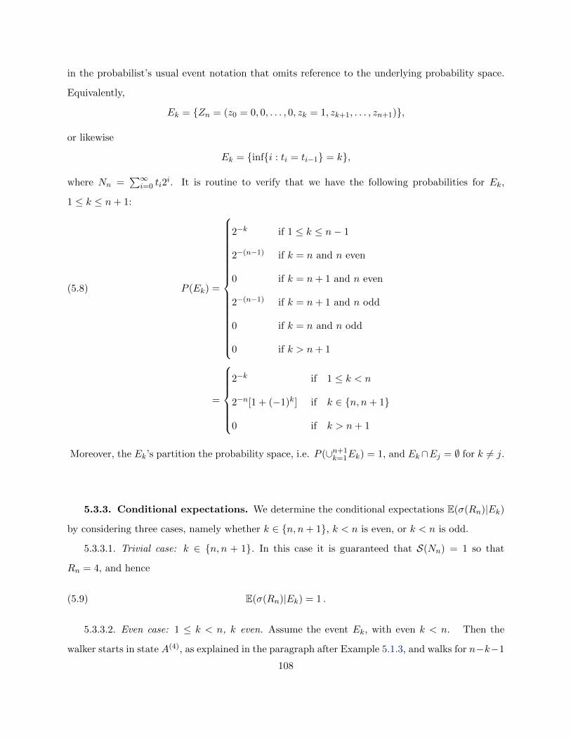
in the probabilist’s usual event notation that omits reference to the underlying probability space.
Equivalently,
Ek = Zn = (z0 = 0, 0, . . . , 0, zk = 1, zk+1, . . . , zn+1),
or likewise
Ek = infi : ti = ti−1 = k,
where Nn =∑∞
i=0 ti2i. It is routine to verify that we have the following probabilities for Ek,
1 ≤ k ≤ n+ 1:
P (Ek) =
2−k if 1 ≤ k ≤ n− 1
2−(n−1) if k = n and n even
0 if k = n+ 1 and n even
2−(n−1) if k = n+ 1 and n odd
0 if k = n and n odd
0 if k > n+ 1
(5.8)
=
2−k if 1 ≤ k < n
2−n[1 + (−1)k] if k ∈ n, n+ 1
0 if k > n+ 1
Moreover, the Ek’s partition the probability space, i.e. P (∪n+1k=1Ek) = 1, and Ek∩Ej = ∅ for k 6= j.
5.3.3. Conditional expectations. We determine the conditional expectations E(σ(Rn)|Ek)
by considering three cases, namely whether k ∈ n, n+ 1, k < n is even, or k < n is odd.
5.3.3.1. Trivial case: k ∈ n, n + 1. In this case it is guaranteed that S(Nn) = 1 so that
Rn = 4, and hence
(5.9) E(σ(Rn)|Ek) = 1 .
5.3.3.2. Even case: 1 ≤ k < n, k even. Assume the event Ek, with even k < n. Then the
walker starts in state A(4), as explained in the paragraph after Example 5.1.3, and walks for n−k−1
108
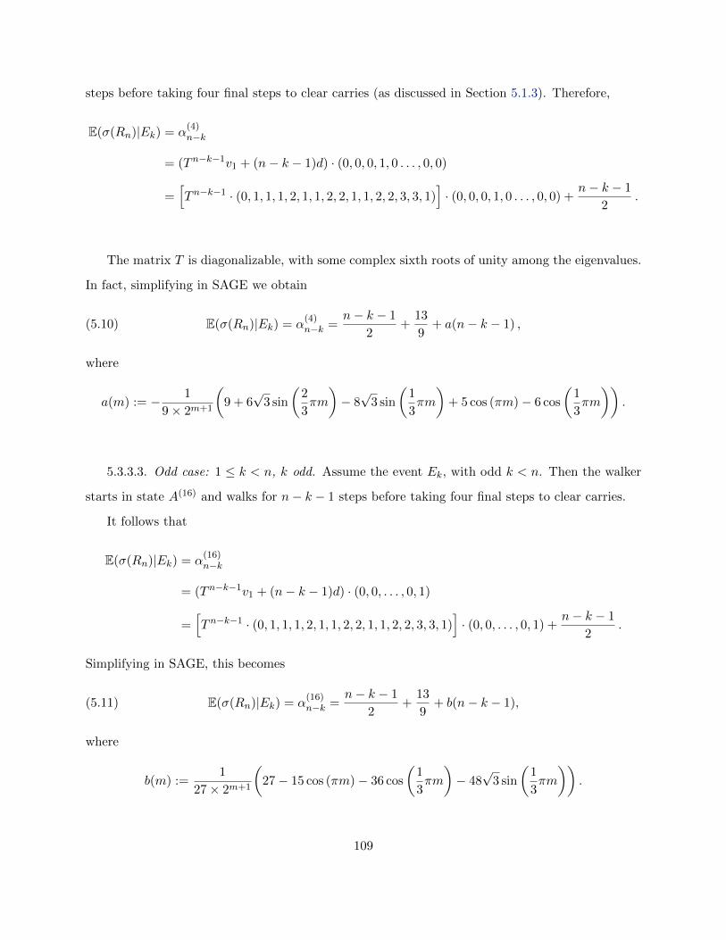
steps before taking four final steps to clear carries (as discussed in Section 5.1.3). Therefore,
E(σ(Rn)|Ek) = α(4)n−k
= (Tn−k−1v1 + (n− k − 1)d) · (0, 0, 0, 1, 0 . . . , 0, 0)
=[Tn−k−1 · (0, 1, 1, 1, 2, 1, 1, 2, 2, 1, 1, 2, 2, 3, 3, 1)
]· (0, 0, 0, 1, 0 . . . , 0, 0) +
n− k − 1
2.
The matrix T is diagonalizable, with some complex sixth roots of unity among the eigenvalues.
In fact, simplifying in SAGE we obtain
(5.10) E(σ(Rn)|Ek) = α(4)n−k =
n− k − 1
2+
13
9+ a(n− k − 1) ,
where
a(m) := − 1
9× 2m+1
(9 + 6
√3 sin
(2
3πm
)− 8√
3 sin
(1
3πm
)+ 5 cos (πm)− 6 cos
(1
3πm
)).
5.3.3.3. Odd case: 1 ≤ k < n, k odd. Assume the event Ek, with odd k < n. Then the walker
starts in state A(16) and walks for n− k − 1 steps before taking four final steps to clear carries.
It follows that
E(σ(Rn)|Ek) = α(16)n−k
= (Tn−k−1v1 + (n− k − 1)d) · (0, 0, . . . , 0, 1)
=[Tn−k−1 · (0, 1, 1, 1, 2, 1, 1, 2, 2, 1, 1, 2, 2, 3, 3, 1)
]· (0, 0, . . . , 0, 1) +
n− k − 1
2.
Simplifying in SAGE, this becomes
(5.11) E(σ(Rn)|Ek) = α(16)n−k =
n− k − 1
2+
13
9+ b(n− k − 1),
where
b(m) :=1
27× 2m+1
(27− 15 cos (πm)− 36 cos
(1
3πm
)− 48√
3 sin
(1
3πm
)).
109

5.3.4. Total expectation. This section is dedicated to the proof of the following proposition,
which, in view of Lemma 5.3.1, will complete the proof of Theorem 1.5.3.
Proposition 5.3.1.
(5.12) E(σ(Rn)) =n+ 1
2− 5
9+
bn9× 2n−1
.
We will reduce the proof of the proposition to the evaluation of an auxiliary function A, which
we define next and then evaluate as a lemma.
Definition 5.3.6. With a and b as in (5.10) and (5.11), define the function A : Z+ → R by
(5.13) A(n) =n−1∑k=2k even
(a(n− k − 1)
1
2k
)+
n−1∑k=1k odd
(b(n− k − 1)
1
2k
),
for n > 2, A(1) = 0, and A(2) = −2/9.
Lemma 5.3.3. For n ≥ 1, we have
A(n) =1 + (−1)n
2n+1+
ρn9× 2n+1
,
where (ρn)∞n=0 := (−10, 0,−34,−48,−58, 12).
We will prove the lemma in the next section. If we assume its validity for now, then we can
verify (5.12) as follows.
Proof of Proposition 5.3.1. Recall the standard total expectation formula for E(σ(Rn)):
E(σ(Rn)) =
n+1∑k=1
E(σ(Rn)|Ek)P (Ek) .
If we substitute into the latter formula the values (5.8) for P (Ek), as well as the values (5.9),
(5.10), and (5.11) for E(σ(Rn)|Ek), then we obtain
110

E(σ(Rn)) =n+1∑k=1
E(σ(Rn)|Ek)P (Ek)(5.14)
=1
2n−1+
n−1∑k=2k even
E(σ(Rn)|Ek)P (EK) +
n−1∑k=1k odd
E(σ(Rn)|Ek)P (Ek)
=1
2n−1+
(n− 1
2+
13
9
)(n−1∑k=1
1
2k
)+
(n−1∑k=1
−k2k+1
)
+n−1∑k=2k even
(a(n− k − 1)
1
2k
)+
n−1∑k=1k odd
(b(n− k − 1)
1
2k
)
=1
2n−1+
(n− 1
2+
13
9
)(1− 1
2n−1
)+
(1
2
)n(n+ 1)− 1 +A(n)
=5
9× 2n−1+
(n+ 1
2− 5
9
)+A(n) ,
where in the second to last inequality we have used the identities∑n−1
k=1 2−k = 1− 21−n and
n−1∑k=1
−k2k+1
=
(1
2
)n(n+ 1)− 1 ,
and the last equality is just simplification. By Lemma 5.3.3, we can rewrite (5.14) as
E(σ(Rn)) =5
9× 2n−1+
(n+ 1
2− 5
9
)+
1 + (−1)n
2n+1+
ρn9× 2n+1
(5.15)
=n+ 1
2− 5
9+
5 + (1 + (−1)n)(9/4) + (ρn/4)
9× 2n−1
=n+ 1
2− 5
9+
ρ′n9× 2n−1
,
where
ρ′n := 5 + (1 + (−1)n)(9/4) + (ρn/4) ,
for n ≥ 0. But it is easy to check that ρ′n = bn for n ≥ 0, so the proof of Proposition 5.3.1 is
complete by virtue of (5.15).
This completes the proof of Theorem 1.5.3, modulo the final task of verifying Lemma 5.3.3,
which we do in the next section.
111
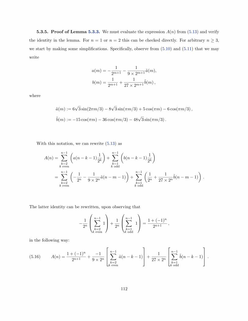
5.3.5. Proof of Lemma 5.3.3. We must evaluate the expression A(n) from (5.13) and verify
the identity in the lemma. For n = 1 or n = 2 this can be checked directly. For arbitrary n ≥ 3,
we start by making some simplifications. Specifically, observe from (5.10) and (5.11) that we may
write
a(m) = − 1
2m+1− 1
9× 2m+1a(m),
b(m) =1
2m+1+
1
27× 2m+1b(m) ,
where
a(m) := 6√
3 sin(2πm/3)− 8√
3 sin(πm/3) + 5 cos(πm)− 6 cos(πm/3) ,
b(m) := −15 cos(πm)− 36 cos(πm/3)− 48√
3 sin(πm/3) .
With this notation, we can rewrite (5.13) as
A(n) =n−1∑k=2k even
(a(n− k − 1)
1
2k
)+
n−1∑k=1k odd
(b(n− k − 1)
1
2k
)
=n−1∑k=2k even
(− 1
2n− 1
9× 2na(n−m− 1)
)+
n−1∑k=1k odd
(1
2n+
1
27× 2nb(n−m− 1)
).
The latter identity can be rewritten, upon observing that
− 1
2n
n−1∑k=2k even
1
+1
2n
n−1∑k=1k odd
1
=1 + (−1)n
2n+1,
in the following way:
(5.16) A(n) =1 + (−1)n
2n+1+−1
9× 2n
n−1∑k=2k even
a(n− k − 1)
+1
27× 2n
n−1∑k=1k odd
b(n− k − 1)
.
112

The lemma’s proof has been reduced then to the evaluation in (5.16) of the two summations
A(n) :=
n−1∑k=2k even
a(n− k − 1)
and
B(n) :=n−1∑k=1k odd
b(n− k − 1) .
We will evaluate them separately and then show that
−1
9× 2nA(n) +
1
27× 2nB(n) =
ρn9× 2n−1
,
which, by (5.16), will imply the desired conclusion that
A(n) =1 + (−1)n
2n+1+
ρn9× 2n−1
,
and thus complete the proof.
5.3.5.1. Evaluation of A(n). Assume n ≥ 3. To evaluate A(n) =
n−1∑k=2k even
a(n− k − 1), we make
the change of variable m = n− k − 1 and write
(5.17) A(n) =n−3∑m=0
n−m odd
a(m) .
Recall that a(m) is the sum of four trigonometric terms. We can express these as periodic
functions of m, as follows:
(6√
3 sin(2πm/3))∞m=0
= (0, 9,−9)(−8√
3 sin(πm/3))∞m=0
= (0,−12,−12, 0, 12, 12)
(5 cos(πm))∞m=0 = (5,−5)
(−6 cos(πm/3))∞m=0 = (−6,−3, 3, 6, 3,−3)
Summing these terms for each m, one finds that (a(m))∞m=0 = (−1,−11,−13, 1, 29,−5) .
113
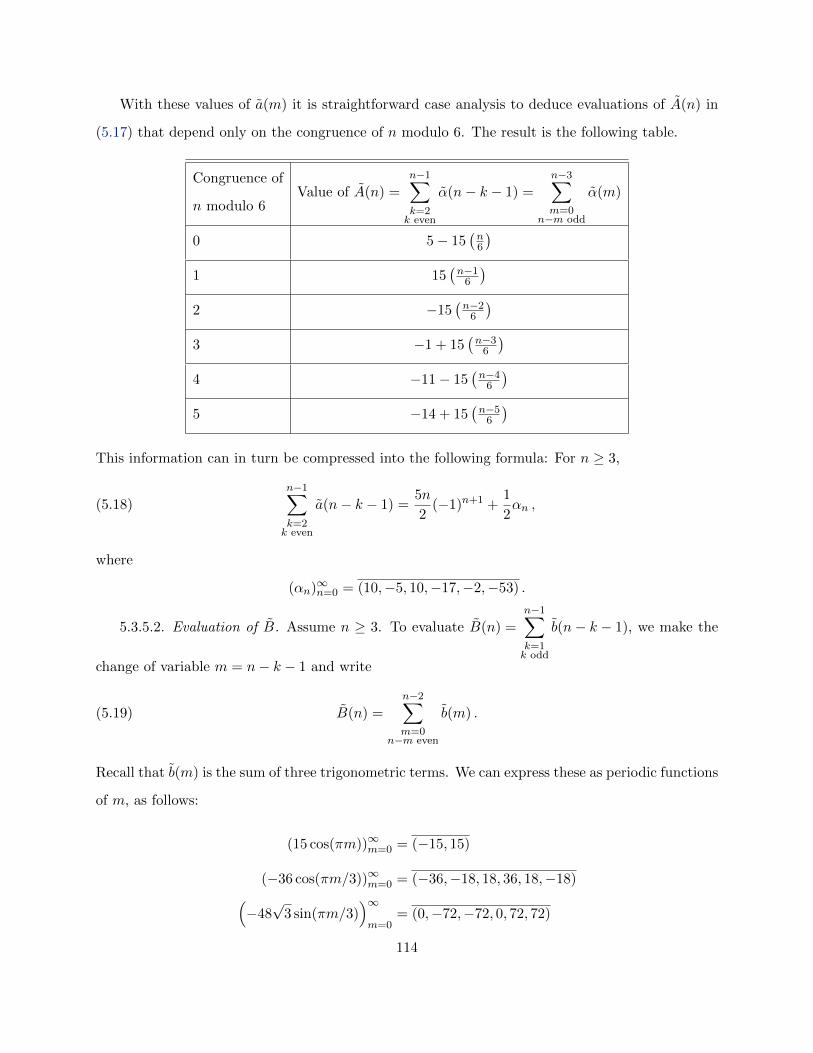
With these values of a(m) it is straightforward case analysis to deduce evaluations of A(n) in
(5.17) that depend only on the congruence of n modulo 6. The result is the following table.
Congruence of
n modulo 6Value of A(n) =
n−1∑k=2k even
α(n− k − 1) =
n−3∑m=0
n−m odd
α(m)
0 5− 15(n6
)1 15
(n−1
6
)2 −15
(n−2
6
)3 −1 + 15
(n−3
6
)4 −11− 15
(n−4
6
)5 −14 + 15
(n−5
6
)This information can in turn be compressed into the following formula: For n ≥ 3,
(5.18)n−1∑k=2k even
a(n− k − 1) =5n
2(−1)n+1 +
1
2αn ,
where
(αn)∞n=0 = (10,−5, 10,−17,−2,−53) .
5.3.5.2. Evaluation of B. Assume n ≥ 3. To evaluate B(n) =
n−1∑k=1k odd
b(n− k − 1), we make the
change of variable m = n− k − 1 and write
(5.19) B(n) =n−2∑m=0
n−m even
b(m) .
Recall that b(m) is the sum of three trigonometric terms. We can express these as periodic functions
of m, as follows:
(15 cos(πm))∞m=0 = (−15, 15)
(−36 cos(πm/3))∞m=0 = (−36,−18, 18, 36, 18,−18)(−48√
3 sin(πm/3))∞m=0
= (0,−72,−72, 0, 72, 72)
114
Summing these terms for each m, one finds that
(b(m))∞m=0 = (−51,−75,−69, 51, 75, 69) .
As we did with A(n), we can evaluate B(n) in (5.19) by considering congruence of n modulo
6. The result is the following table.
Congruence of
n modulo 6Value of B(n) =
n−1∑k=1k odd
b(n− k − 1) =
n−2∑m=0
n−m even
b(m)
0 −45(n6
)1 45
(n−1
6
)2 −51− 45
(n−2
6
)3 −75 + 45
(n−3
6
)4 −120− 45
(n−4
6
)5 −24 + 45
(n−5
6
)This information can be compressed into the following formula: For n ≥ 3,
(5.20)n−1∑k=1k odd
b(n− k − 1) =15n
2(−1)n+1 +
1
2βn ,
where
(βn)∞n=0 = (0,−15,−72,−195,−180,−123) = 3× (0,−5,−24,−65,−60,−41) .
5.3.5.3. Evaluation of A(n). Recall from (5.16) that
A(n) =1 + (−1)n
2n+1+−1
9× 2nA(n) +
1
27× 2nB(n) .
In view of (5.18) and (5.20), we have
−1
9× 2nA(n) +
1
27× 2nB(n) =
1
9× 2n+1(−αn + βn/3) .
Since −αn + βn/3 = ρn, the proof of Lemma 5.3.3 is complete.
115

Bibliography
[And76] G. Andrews, The Theory of Partitions, Addison-Wesley Publishing Company, 1976.
[Bai35] W. Bailey, Generalized Hypergeometric Series, Cambridge University Press, 1935.
[BD15] C. Banderier and M. Drmota, Formulae and asymptotics for coefficients of algebraic functions, Combina-
torics, Probability and Computing 24 (2015), 1–53.
[Bel61] R. Bellman, A Brief Introduction to Theta Functions, Holt, Rinehart and Winston, Inc, 1961.
[BTWZ19] A. Bostan, J. Tirrell, B. Westbury, and Y. Zhang, On sequences associated to the invariant theory of rank
two simple Lie algebras, 2019, 1911.10288.
[Coh17] H. Cohn, A conceptual breakthrough in sphere packing, Not. Amer. Math. Soc. 64 (2017), 102–115.
[Dar78] J.-G. Darboux, Memoire sur l’approximation des fonctions de tres grands nombres, et sur une classe
etendu de d’eveloppements en serie, Journal de Math. Pures et Appliquees 3 (1878), no. 4, 5–56.
[DB58] N. De Bruijn, Asymptotic Methods in Analysis, North-Holland Publishing Company, 1958.
[DF04] D. Dummit and R. Foote, Abstract Algebra (3rd ed.), John Wiley and Sons, Inc., 2004.
[DG08] B. Datskovsky and P. Guerzhoy, P-adic interpolation of Taylor coefficients of modular forms, Math. Ann.
340 (2008), no. 2, 465–476.
[Drm04] M. Drmota, Combinatorics and asymptotics on trees, CUBO, A Mathematical Journal 6 (2004), no. 2,
105–136.
[DS16] F. Diamond and J. Shurman, A First Course in Modular Forms, Springer, 2016.
[Fek23] M. Fekete, Uber die verteilung der wurzeln bei gewissen algebraischen gleichungen mit ganzzahligen koef-
fizienten, Mathematische Zeitschrift 17 (1923), no. 1, 228–249.
[Fin78] H. Finkelstein, Solving equations in groups: a survey of Frobenius’ theorem, Periodica Mathematica
Hungarica 9 (1978), no. 3, 187–476.
[FO90] P. Flajolet and A. Odlzyko, Singularity analysis of generating functions, SIAM J. Discrete Math. 3 (1990),
no. 2, 216–240.
[FS09] P. Flajolet and R. Sedgewick, Analytic Combinatorics, Cambridge University Press, 2009.
[GM93] D. Grabiner and P. Magyar, Random walks in Weyl chambers and the decomposition of tensor powers,
Journal of Algebraic Combinatorics 2 (1993), 216–240.
[GMR20] P. Guerzhoy, M. Mertens, and L. Rolen, Periodicities for Taylor coefficients of half-integral weight modular
forms, Pacific J. of Math 307 (2020), 137–157.
116

[GZ92] I. Gessel and D. Zeilberger, Random walks in a Weyl chamber, Proc. Amer. Math. Soc. 115 (1992), no. 1,
27–31.
[Hil59] E. Hille, Analytic Function Theory, vol. 1, Ginn and Company, 1959.
[Hum72] J. Humphreys, Introduction to Lie Algebras and Representation Theory, Springer, 1972.
[KL03] I. Krasikov and J. Lagarias, Bounds for the 3x+ 1 problem using difference inequalities, Acta Arith 109
(2003), no. 3, 237–258.
[Kob93] N. Koblitz, Introduction to Elliptic Curves and Modular Forms, 2nd ed., Springer, 1993.
[Kup94] G. Kuperberg, The quantum G2 link invariant, Internat. J. Math. 5 (1994), no. 1, 61–85.
[Kup96] , Spiders for rank 2 Lie algebras, Comm. Math. Phys. 180 (1996), no. 1, 109–151.
[Lag85] J. Lagarias, The 3x+ 1 problem and its generalizations, The American Mathematical Monthly 92 (1985),
3–23.
[Lag10] The Ultimate Challenge: The 3x+ 1 Problem, (J. Lagarias, ed.), American Math. Society, 2010.
[Lan02] S. Lang, Algebra (3rd ed.), Springer Science + Business Media LLC, 2002.
[Leg08] A. Legendre, Essai sur la theorie des nombres (2nd ed.), Paris, Chez Courcier, Imprimeur - Libraire pour
les Mathematiques, quai des Augustins, no 57, 1808.
[LS14] H. Larson and G. Smith, Congruence properties of Taylor coefficients of modular forms, Int. J. Number
Theory 10 (2014), 1504–1518.
[Mat10] K. Matthews, Generalized 3x + 1 mappings: Markov chains and ergodic theory, In: The Ultimate Chal-
lenge: The 3x+ 1 Problem (J. Lagarias, ed.), American Math. Society, 2010, pp. 79–103.
[MM78] A. Meir and J. Moon, On the altitude of nodes in random trees, Can. J. Math 30 (1978), no. 5, 997–1015.
[MM89] A. Meir and J. Moon, On an asymptotic method in enumeration, J. of Combinatorial Number Theory,
Series A 51 (1989), no. 1, 77–89.
[Pol37] G. Polya, Polya, george. kombinatorische anzahlbestimmungen fur gruppen, graphen und chemische
verbindungen., Acta Math. 68 (1937), 145–254.
[Rom20] D. Romik, The Taylor coefficients of the Jacobi theta constant θ3, Ramanujan Journal 52 (2020), 275–290.
[RS] D. Romik and R. Scherer, Identities for average values of iterates of the Syracuse map, in preparation.
[RS20] , Alternative summation orders for the Eisenstein series G2 and Weierstrass ℘-function, Rocky
Mountain J. Math 50 (2020), no. 4, 1473–1482.
[Sch20] R. Scherer, A criterion for sharpness in tree enumeration and the asymptotic number of triangulations in
Kuperberg’s G2 spider, 2020, https://arxiv.org/pdf/2003.07984.pdf.
[Sch21] , Congruences modulo primes of the Romik sequence related to the Taylor expansion of the Jacobi
theta constant θ3, Ramanujan Journal 54 (2021), 427–448.
[Shi73] G. Shimura, On modular forms of half integral weight, Annals of Math. 97 (1973), no. 3, 440–481.
[SI20] N. J. A. Sloane and T. O. F. Inc., The On-line Encyclopedia of Integer Sequences, online source, accessed
April 2020, http://oeis.org.
117

[Smi59] K. Smith, Analytic Function Theory, vol. 1, Ginn and Company, 1959.
[SS03] E. Stein and R. Shakarchi, Complex Analysis (Princeton Lectures in Analysis, no. 2), Princeton University
Press, 2003.
[Sta99] R. Stanley, Enumerative Combinatorics, vol. 2, Cambridge University Press, 1999.
[Tao20] T. Tao, Almost all orbits of the Collatz map attain almost bounded values, 2020, 1909.03562v3.
[TZ04] T. Tate and S. Zeldtich, Lattice path combinatorics and asymptotics of multiplicities of weights in tensor
powers, Journal of Functional Analysis 217 (2004), no. 2, 402–447.
[VD93] F. Villegas and Z. D, Square roots of central values of Hecke L-series, In: Advances in Number Theory
(F. Gouvea and N. Yui, eds.), Clarendon Press, 1993, pp. 81–99.
[Via17] M. Viazovska, The sphere packing problem in dimension 8., Ann. Math 185 (2017), 991–1015.
[Wak20] T. Wakhare, Romik’s conjecture for the Jacobi theta function, J. of Number Theory 215 (2020), no. 2,
275–296.
[Wes07] B. Westbury, Enumeration of non-positive planar trivalent graphs, Journal of Algebraic Combinatorics
25 (2007), no. 4, 357–373.
[Wol20] Wolfram Research, online source, accessed Oct. 2020, https://functions.wolfram.com/Hypergeometric
Functions/Hypergeometric2F1/06/01/04/01/02.
[Woo86] D. Wood, Theory of Computaiton, Wiley, 1986.
[Zag89] D. Zagier, Introduction to Modular Forms, In: From Number Theory to Physics (M. Waldschmidt,
P. Moussa, J.-M. Luck, and C. Itzykosn, eds.), Springer-Verlag, 1989, pp. 238–291.
[Zag08] , Elliptic Modular Forms and Their Applications, In: The 1-2-3 of modular forms (K. Ranestad,
ed.), Springer, 2008, pp. 1–103.
118
Top Related