


Languages
Pages
Legal


Time Series Matching:
a Multi-filter Approach
by
Zhihua Wang
A dissertation submitted in partial fulfillment
of the requirements for the degree of
Doctor of Philosophy
Department of Computer Science
Courant Institute of Mathematical Sciences
New York University
January 2006
Dennis Shasha

c© Zhihua Wang
All Rights Reserved, 2006


Dedicated to my dear parents Limao Wang, Dejun Zhu
and my lovely wife Nina Liu who blessed and supported me
iv

Acknowledgments
Many thanks to my adviser Professor Dennis Shasha for all of his kind help
with my work as well as advice from Professor Richard Cole, Professor Yann
Lecun and Professor Panayotis Mavromatis. Additional thanks to Dr. Naoko
Kosugi, Dr. Yunyue Zhu and Xiaojian Zhao for their generous help and to other
team members of the Query by Humming project for their hard work: Kenji
Yoshihira, Kevin Cox, I-Hsiu Lee and Marc-olivier Caillot. Also, great thanks
to many people who contributed humming: Anina Karman, Professor Clifford
M. Hurvich, Dr. David Tanzer, Professor Foster Provost, Karen Shasha, Maria
Petagna, Dr. M. Alex O. Vasilescu and web users from all over the world.
Finally thanks to Katharine Rose Sabo for her editing help.
v

Abstract
Data arriving in time order (time series) arises in disciplines ranging from music
to meteorology to finance to motion capture data, to name a few. In many cases,
a natural way to query the data is what we call time series matching - a user
enters a time series by hand, keyboard or voice and the system finds “similar”
time series.
Existing time series similarity measures, such as DTW (Dynamic Time
Warping), can accommodate certain timing errors in the query and perform
with high accuracy on small databases. However, they all have high computa-
tional complexity and the accuracy drops dramatically when the data set grows.
More importantly, there are types of errors that cannot be captured by a single
similarity measure.
Here we present a general time series matching framework. This frame-
work can easily optimize, combine and test different features to execute a fast
similarity search based on the application’s requirements. Basically we use a
multi-filter chain and boosting algorithms to compose a ranking algorithm. Each
filter is a classifier which removes bad candidates by comparing certain features
of the time series data. Some filters use a boosting algorithm to combine a
few different weak classifiers into a strong classifier. The final filter will give a
ranked list of candidates in the reference data which matches the query data.
vi

The framework is applied to build query algorithms for a Query-by-Humming
system. Experiments show that the algorithm has a more accurate similarity
measure and its response time increases much more slowly than the pure DTW
algorithm when the number of songs in the database increases from 60 to 1400.
vii

Contents
Dedication iv
Acknowledgments v
Abstract vi
List of Figures x
List of Appendices xii
1 Introduction 1
1.1 Motivation . . . . . . . . . . . . . . . . . . . . . . . . . . . . . . 1
1.2 Problem Statement . . . . . . . . . . . . . . . . . . . . . . . . . 2
1.3 Our Contribution . . . . . . . . . . . . . . . . . . . . . . . . . . 3
1.4 Thesis Outline . . . . . . . . . . . . . . . . . . . . . . . . . . . . 3
2 Underlying Technology 5
2.1 Brief Overview . . . . . . . . . . . . . . . . . . . . . . . . . . . 5
2.2 GEMINI framework . . . . . . . . . . . . . . . . . . . . . . . . . 6
2.3 Dynamic Warping Distance Measure (DTW) . . . . . . . . . . . 8
2.4 Indexing the DTW distance . . . . . . . . . . . . . . . . . . . . 13
viii

2.5 Data Preparation . . . . . . . . . . . . . . . . . . . . . . . . . . 21
2.6 Summary . . . . . . . . . . . . . . . . . . . . . . . . . . . . . . 24
3 Time Series Matching Framework 25
3.1 Formal Problem Statement . . . . . . . . . . . . . . . . . . . . . 26
3.2 Framework Overview . . . . . . . . . . . . . . . . . . . . . . . . 27
3.3 Functionalities . . . . . . . . . . . . . . . . . . . . . . . . . . . . 28
3.4 Framework Components . . . . . . . . . . . . . . . . . . . . . . 33
3.5 Component Examples . . . . . . . . . . . . . . . . . . . . . . . . 38
3.6 Usage Examples . . . . . . . . . . . . . . . . . . . . . . . . . . . 46
3.7 Summary . . . . . . . . . . . . . . . . . . . . . . . . . . . . . . 47
4 Case Study: Query-by-humming 48
4.1 Related Work Review . . . . . . . . . . . . . . . . . . . . . . . . 49
4.2 Our Query-by-humming System . . . . . . . . . . . . . . . . . . 54
4.3 Building the algorithm . . . . . . . . . . . . . . . . . . . . . . . 59
4.4 Evaluating the algorithm . . . . . . . . . . . . . . . . . . . . . . 72
4.5 Future Work . . . . . . . . . . . . . . . . . . . . . . . . . . . . . 78
5 Conclusion 80
Appendices 81
Bibliography 93
ix

List of Figures
2.1 GEMINI framework . . . . . . . . . . . . . . . . . . . . . . . . . 7
2.2 Dynamic Time Warping (from [37]) . . . . . . . . . . . . . . . 8
2.3 DTW distance computation (from [37]) . . . . . . . . . . . . . . 9
2.4 DTW distance with global constraints (figure from [14]) . . . . . 11
2.5 Envelope of a time series (figure from [14]) . . . . . . . . . . . . 14
2.6 Transformed Envelope of a time series (figure from [37]) . . . . . 17
2.7 The PAA transformation (figure from [16]) . . . . . . . . . . . . 20
3.1 Multi-filter algorithm structure . . . . . . . . . . . . . . . . . . 27
3.2 Ada boosting . . . . . . . . . . . . . . . . . . . . . . . . . . . . 30
3.3 Framework components from bottom to top . . . . . . . . . . . 34
4.1 New Query-by-humming System . . . . . . . . . . . . . . . . . . 54
4.2 Compare humming using ‘ta’ and ‘la’ . . . . . . . . . . . . . . . 56
4.3 Good global alignment, bad local alignment . . . . . . . . . . . 58
4.4 The distribution of the measures based on the number of notes . 61
4.5 The distribution of note values’ standard deviation . . . . . . . 63
4.6 Compare the direction change count and zero-crossing rate . . . 64
4.7 The distribution of the ratio of most significant value . . . . . . 66
4.8 The distribution of the max-min value difference . . . . . . . . . 67
x

4.9 The distribution of the LDTW measure on the first 5 values . . 68
4.10 The distribution of the LDTW measures using different order . 70
4.11 Compares the hit-rate to pure DTW distance measure . . . . . 74
4.12 Compares the response time to pure DTW distance measure . . 75
4.13 Compare the hit-rate’s scalability . . . . . . . . . . . . . . . . . 76
4.14 Compare the response time’s scalability . . . . . . . . . . . . . . 77
C.1 Google search result top-1 with keywords “query by humming” . 88
C.2 Yahoo search result top-1 with keywords “query by humming” . 89
C.3 MSN search result top-1 with keywords “query by humming” . . 90
C.4 Screenshot of the web demo . . . . . . . . . . . . . . . . . . . . 91
C.5 Screenshot of the Java GUI client . . . . . . . . . . . . . . . . . 92
xi

List of Appendices
Appendix A Boosting Algorithm 81
Appendix B Components Examples 83
Appendix C Feedback on the system 88
xii

Chapter 1
Introduction
1.1 Motivation
Many applications naturally generate time series data. The research on time
series matching is becoming increasingly popular as more and more applications
emerge and the sizes of data increase dramatically. For example:
• Millions of traders try to find patterns by tracking similar stocks using the
up to 100,000 quotes and trades (ticks) which are generated per second in
the United States;
• Meteorologists try to predict weather based on similarities between cloud
movements using new satellites (launched last year) which collect 3GB of
data every day;
• Many real-time 3D games today need a way to automate a virtual charac-
ter’s transition movement; using a motion-captured animation database,
the next motion sequence is selected from the motions whose beginning
matches the ending of the current motion.
1

As the above examples illustrate, the most convenient way to investigate the
data is by using existing examples as queries to find similar data.
Existing time series matching similarity measure, such as DTW (Dynamic
Time Warping) [37], can accommodate certain timing errors in the query and
perform similarity search with high accuracy when matching queries to small
databases. However, they all have high computational complexity and the accu-
racy drops dramatically when the data set grows. In short, they don’t scale well.
Another problem is that the type and amount of time warping may be differ-
ent for different applications. There is a need for scalable matching algorithms
which can be easily customized for different applications.
1.2 Problem Statement
In summary, there are two major difficulties for the time series matching prob-
lem.
• First is the error in the query and the ambiguity of similarity
There should be either an accurate definition of similarity measure be-
tween data or a system that can learn this similarity measure. This way
users can find the data they really need.
• Second is the large scale of the database
The more data, the more difficult it is to discriminate the correct result
from other ones and the greater the challenge of giving an accurate defini-
tion of similarity. Additionally, the larger the scale, the more computation
power needed and the more efficient the query algorithm must be.
2

This thesis will address both of these challenges. It will discuss how to build
fast, accurate and customizable similarity search algorithms for large scale time-
series systems that allow for errors in the query.
1.3 Our Contribution
We will present a general time series matching framework. This frame-
work can easily optimize, combine and test different features to conduct fast
similarity searches based on the requirements of the application. It takes a
multi-filter approach plus Boosting [11, 25] to compose a ranking algorithm.
Both theoretical discussions and experimental results are presented.
1.4 Thesis Outline
We first review related work and common techniques; this includes the GEMINI
indexing framework and the most commonly used template matching algorithm,
Dynamic Time Warping (DTW) [20, 37].
Second, we present the time series matching framework. This framework is
designed and implemented to address both the ambiguity of the query and the
large scale of the database with emphasis on finding the best similarity measure.
The idea is to extract and compare different features of the time series data,
then configure a composite of features to efficiently measure the similarity be-
tween a specific type of the data. The selection of features is based on the time
complexity and discriminating power of the different features and the charac-
teristics of the data. This framework can easily optimize the parameters of the
new features as well as combine them into comprehensive similarity measure
3

algorithms.
Third, a concrete application example of a Query-by-Humming system is
studied in detail. This music retrieval application is built based on the time
series matching framework. A Query-by-Humming system enables the user
to find songs by humming part of the tune. In our system, both music and
humming are represented as time series data. Thus we can directly use the
time series matching framework to build a similarity algorithm with the goal of
maximizing the music recognition percentage for the humming we collected.
In this case study, we first review techniques specifically related to music
information retrieval; second, we present our algorithm architecture and com-
pare the results with other systems. Finally, we conclude the thesis and discuss
possible directions for future work.
4

Chapter 2
Underlying Technology
2.1 Brief Overview
There are a few important works related to time series matching. Here we
provide a brief overview followed by a detailed discussion of each technique.
1. GEMINI framework and related transformations techniques
GEMINI framework theory[10] essentially transforms the data into
a lower-dimension and speeds up the matching process. Various trans-
formation techniques have been developed, mainly for Euclidean distance
comparison. Each transformation guarantees no false negatives and has a
different computational complexity and tightness of lower-bounding.
2. DTW and related indexing techniques
Dynamic Time Warping (DTW) [5] is a similarity matching technique
that allows alignment shifting between time series. The DTW distance
does not satisfy the triangle inequality, so special transformation tech-
niques are developed to speed up the matching process and guarantee no
5

false negatives. These kinds of transformations act as indexing techniques
which reduce comparison computational complexity.
Besides the framework and indexing techniques, preprocessing tech-
niques which normalize the data are important to make sure that the com-
parison makes sense.
2.2 GEMINI framework
Similarity querying for time series databases has been a topic of research in
the database community for many years. A lot of work used Euclidean distance
between time series as a similarity measure [3, 10, 23, 36, 7, 22, 32, 17, 33, 15, 34].
They can all be applied in the GEMINI framework introduced by Christos
Faloutsos, M Ranganathan and Yannis Manolopoulos [10].
The key concept of the GEMINI framework (Figure 2.1) is to first map each
time series to a lower dimension, then find similar ones by looking them up in a
multidimensional index structure and finally, compare those time series in the
original space. The important thing is that the transformations should satisfy
the lower-bounding property:
• Lower-Bounding
Dindex−space(x, y) ≤ Dtrue(x, y) (2.1)
Lower-Bounding means the distance between each of the transformed time
series should be less than the distance between each of the original time series.
• No false negatives
6

Syn(s2) in indexSyn(s1) in index
to close points in the index.
if their synopses map
are probably close
s1 and s2
Store in
index structure.
multidimensional
Synopsis of s2Synopsis of s1
Time Series s2Time Series s1
Figure 2.1: GEMINI framework
With the lower-bounding property, the GEMINI framework guarantees no
false negatives: any time series that is similar to the query in the original space
will be selected by the indexing structure. False negatives refer to the situation
that discards reference data which are actually similar to the query datum;
similarly, true negatives refer to the discarded reference data that are not similar
to the query datum.
• Tightness of Lower-Bounding
The differences among the works cited above is that they used different
transformations to satisfy the lower-bounding property. The tightness of lower-
bounding determines the performance of the transformations.
7

Assume we define:
T =Dindex−space
Dtrue
T is in the range of [0, 1] and a larger T gives a tighter bound. The tighter
the bound, the better the distance in the transformed space approximates the
distance in the original space, thus the better the pruning power of the indexing.
2.3 Dynamic Warping Distance Measure (DTW)
Time Series 1Time Series 2
Figure 2.2: Dynamic Time Warping (from [37])
Although the Euclidean distance is used as a similarity measure in a lot of
work, it is not suitable for cases where the time series are out of phase in the
time axis, see Figure 2.2 for an example. The two time series look similar but
they are not close in Euclidean distance. As a solution to this, D. Berndt and J.
Clifford [5] introduced DTW into the database community. The Dynamic Time
Warping (DTW) distance is a much more robust distance measure for similarity
8
matching which allows alignment shifting between time series. For the two time
series in Figure 2.2, the DTW distance is much smaller than their Euclidean
distance.
2.3.1 Definition of DTW Distance
The Dynamic Time Warping distance between two time series x, y is
D2DTW (x, y) = D2(First(x), F irst(y)) + min
D2DTW (x, Rest(y))
D2DTW (y, Rest(x))
D2DTW (Rest(x), Rest(y))
where First(x) is the first element of x, and Rest(x) is the remainder of the
time series after the First(x) has been removed.
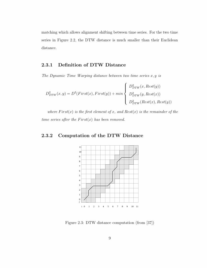
2.3.2 Computation of the DTW Distance
4.1 Uniform time warping
0 1 2
0
1
2
3
4
5
6
7
8
9
10
11
3 4 5 6 7 8 9 10 11
j
i
4.2 Local dynamic time warping
Figure 2.3: DTW distance computation (from [37])
9

The process of computing the DTW distance can be visualized as a string
matching style dynamic program, see Figure 2.3. For time series x of length n
and time series y of length m, we use an n × m matrix M to align them. The
cell Mi,j corresponds to the alignment of element xi and yj. Any monotonic and
continuous path P from M0,0 to Mn−1,m−1 forms a particular alignment between
x and y:
P = p1, p2, . . . , pl = (px1 , p
y1), (p
x2, p
y2), . . . , (p
xl , p
yl )
max(n, m) ≤ l ≤ n + m − 1
and
• P is monotonic if pxt − px
t−1 ≥ 0 and pyt − py
t−1 ≥ 0
• P is continuous if pxt − px
t−1 ≤ 1 and pyt − py
t−1 ≤ 1
If we associate each cell alignment with its corresponding cost, say D2(i, j),
then the sum of the cost along a path represents the cost of the particular align-
ment. One can prove that the minimum path cost for all possible alignments is
the DTW distance between x and y. The minimum-cost path also determines
the optimal alignment between x and y.
The time computation cost for DTW distance is O(mn) using Dynamic
Programming [37].
2.3.3 Variants of DTW
Usually we add constraints to DTW to avoid too much flexibility in the warping.
Two popular global constraints are Sakoe-Chiba Band and Itakura Parallelo-
10

difference of their value and the maximum (minimum)
value of the other sequence to the final DTW distance.
Figure 5 illustrates the idea.
Figure 5: A visual intuition of the lower bounding measure
introduced by Yi et al. The sum of the squared length of
gray lines represent the minimum the corresponding points
contribution to the overall DTW distance, and thus can be
returned as the lower bounding measure
3.3 Proposed lower bounding measure
Before introducing our lower bounding technique we
must review an additional detail of the DTW algorithm
that we deliberately omitted until now.
3.3.1 Global constraints on time warping
In addition to the constraints on the warping path
enumerated in Section 2.2, virtually all practitioners using
DTW also constraint the warping path in a global sense
by limiting how far it may stray from the diagonal [3].
The subset of matrix that the warping path is allowed to
visit is called the warping window. Figure 6 illustrates
two of the most frequently used global constraints, the
Sakoe-Chiba Band and the Itakura Parallelogram [27, 29].
Figure 6: Global constraints limit the scope of the warping
path, restricting them to the gray areas. The two most
common constraints in the literature are the Sakoe-Chiba
Band and the Itakura Parallelogram
There are several reasons for using global constraints,
one of which is that they slightly speed up the DTW
distance calculation. However the most important reason
is to prevent pathological warpings, where a relatively
small section of one sequence maps onto a relatively large
section of another. The importance of global constraints
was documented by the originators of the DTW
algorithm, who where exclusively interested in aligning
speech patterns [29]. However, has been empirically
confirmed in other settings, including finance, medicine,
biometrics, chemistry, astronomy, robotics and industry.
0 5 10 15
20 25
30 35
40
max(Q)
min(Q)
As a motivating example consider the two sequences
in Figure 1 which were used to illustrate DTW. The
smooth peaks in each correspond to increase in demand
for electrical power during weekdays. In the topmost
sequence there is no peak on Monday because it was a
national holiday, the same is true for Wednesday in the
bottom sequence. In this domain, we may well decide that
that it makes sense to allow warpings of up to one day, i.e.
Monday may warp to Tuesday and Tuesday may warp to
Wednesday etc, but more drastic warpings (i.e. Monday to
Friday) should not be allowed. This constraint can easily
be enforced by using a Sakoe-Chiba Band with a width
equal to n/7.
3.3.2 Proposed lower bounding measure
We can view a global constraint as constraining the
indices of the warping path wk = (i,j)k such that j-r i
j+r where r is a term defining the reach, or allowed range
of warping, for a given point in a sequence. In the case of
the Sakoe-Chiba Band r is independent of i, for the
Itakura Parallelogram r is a function of i.
We will use the term r to define two new sequences, U
and L:
Ui = max(qi-r : qi+r) (6)
Li = min(qi-r : qi+r) (7)
U and L stand for Upper and Lower respectively, we
can see why if we plot them together with the original
sequence Q as in Figure 7. They form a bounding
envelope that encloses Q from above and below. Note that
although the Sakoe-Chiba Band is of constant width, the
corresponding envelope generally is not of uniform
thickness. In particular, the envelope is wider when the
underlying query sequence is changing rapidly, and
narrower when the query sequence plateaus.
C
Q
C
Q
Sakoe-Chiba Band Itakura Parallelogram
U
L
0 5 10 15 20 25 30 35 40
L
A
B
U
Q
Q
Figure 7: An illustration of the sequences U and L, created
for sequence Q (shown dotted). A was created using the
Sakoe-Chiba Band and B using the Itakura Parallelogram
Figure 2.4: DTW distance with global constraints (figure from [14])
gram constraints, illustrated in Figure 2.4. Alignments of cells can be selected
only from the shaded area. The Sakoe-Chiba Band constraint is also called
k-Local Dynamic Time Warping (k-LDTW ). With k-LDTW, the ith element
of x can be aligned only to one of the k nearest elements of y.
k-LDTW Distance
The k-LDTW between two time series x, y is
D2LDTW (k)(x, y) = D2
constraint(k)(First(x), F irst(y))
+min
D2LDTW (k)(x, Rest(y))
D2LDTW (k)(y, Rest(x))
D2LDTW (k)(Rest(x), Rest(y))
(2.2)
where
D2constraint(k)(xi, yj) =
D2(xi, yj) if |i − j| ≤ k
∞ if |i − j| > k
11

α%-LDTW Distance
The α%-LDTW distance of x and y is equivalent to the k-LDTW distance
where k is the production of the α% and the larger value between the x and y’s
lengths.
Other variants of DTW have been introduced to accommodate different
situations. Selina Chu, Eamonn Keogh, David Hart and Michael Pazzani [9] in-
troduced an iterative deepening DTW which automatically adjusts the warping
parameter based on user specified tolerance for the probability of false dismissal.
C. A. Ratanamahatana and E. Keogh [24] added a machine learning tech-
nique to DTW, so that each datum in the database had a learned constraint
to be applied during the DTW distance computation. In this way, both the
accuracy and efficiency are improved, although the learning process is compu-
tationally expensive. This method generally requires a large number of training
samples, so it has limited applications.
More general variants of DTW are discussed in Sergios Theodoridis and
Konstantinos Koutroumbas’s book Pattern Recognition [29]. These include ap-
plying different local or global constraints and allowing the omission or insertion
of data elements.
2.3.4 Advantages and Disadvantages
One advantage of DTW is that the DTW distance measure is less sensitive to
local time shift distortion than the Euclidean distance measure. Also, it can
handle time series of various lengths while the Euclidean distance measure can
compare only equal length time series.
However, the cost of the DTW distance computation is much higher than
12

that of the Euclidean distance computation, which is O(n) if both time series are
of length n. Secondly, the DTW distance does not obey the triangle inequality
and it is difficult to index precisely.
Triangle Inequality
A distance measure D satisfies triangle inequality if:
D(x, y) ≤ D(x, z) + D(y, z), for any data x, y, z
“Virtually all techniques to index data require the triangle inequality to
hold.” [13]
A very simple example that DTW distance does not obey the triangle in-
equality is as follows:
Suppose there are three time series data x, y, z where
x = 1, 1, 1, 2, 2, 2
y = 1, 1, 2, 2, 2, 2
z = 1, 1, 1, 1, 2, 2
The local DTW distances between them with 5%-warping are D(x, y) = 0,
D(x, z) = 0 and D(y, z) =√
2. Thus D(y, z) > D(x, y) + D(x, z) where it does
not obey the triangle inequality.
2.4 Indexing the DTW distance
Despite the fact that DTW distance still does not satisfy the triangle inequality,
Keogh’s paper [14] proposed a novel indexing technique by introducing envelope
filtering and transformed envelope filtering to exactly index the DTW distance.
13

Y. Zhu, D. Shasha, X. Zhao [37] further generalized the idea into a GEM-
INI framework for the DTW distance measure by introducing the container-
invariant property of the transformations. They also improved the pruning
power of the indexing by introducing a transformation which gives a tighter
lower-bounding.
2.4.1 Envelope Filter
difference of their value and the maximum (minimum)
value of the other sequence to the final DTW distance.
Figure 5 illustrates the idea.
Figure 5: A visual intuition of the lower bounding measure
introduced by Yi et al. The sum of the squared length of
gray lines represent the minimum the corresponding points
contribution to the overall DTW distance, and thus can be
returned as the lower bounding measure
3.3 Proposed lower bounding measure
Before introducing our lower bounding technique we
must review an additional detail of the DTW algorithm
that we deliberately omitted until now.
3.3.1 Global constraints on time warping
In addition to the constraints on the warping path
enumerated in Section 2.2, virtually all practitioners using
DTW also constraint the warping path in a global sense
by limiting how far it may stray from the diagonal [3].
The subset of matrix that the warping path is allowed to
visit is called the warping window. Figure 6 illustrates
two of the most frequently used global constraints, the
Sakoe-Chiba Band and the Itakura Parallelogram [27, 29].
Figure 6: Global constraints limit the scope of the warping
path, restricting them to the gray areas. The two most
common constraints in the literature are the Sakoe-Chiba
Band and the Itakura Parallelogram
There are several reasons for using global constraints,
one of which is that they slightly speed up the DTW
distance calculation. However the most important reason
is to prevent pathological warpings, where a relatively
small section of one sequence maps onto a relatively large
section of another. The importance of global constraints
was documented by the originators of the DTW
algorithm, who where exclusively interested in aligning
speech patterns [29]. However, has been empirically
confirmed in other settings, including finance, medicine,
biometrics, chemistry, astronomy, robotics and industry.
0 5 10 15
20 25
30 35
40
max(Q)
min(Q)
As a motivating example consider the two sequences
in Figure 1 which were used to illustrate DTW. The
smooth peaks in each correspond to increase in demand
for electrical power during weekdays. In the topmost
sequence there is no peak on Monday because it was a
national holiday, the same is true for Wednesday in the
bottom sequence. In this domain, we may well decide that
that it makes sense to allow warpings of up to one day, i.e.
Monday may warp to Tuesday and Tuesday may warp to
Wednesday etc, but more drastic warpings (i.e. Monday to
Friday) should not be allowed. This constraint can easily
be enforced by using a Sakoe-Chiba Band with a width
equal to n/7.
3.3.2 Proposed lower bounding measure
We can view a global constraint as constraining the
indices of the warping path wk = (i,j)k such that j-r i
j+r where r is a term defining the reach, or allowed range
of warping, for a given point in a sequence. In the case of
the Sakoe-Chiba Band r is independent of i, for the
Itakura Parallelogram r is a function of i.
We will use the term r to define two new sequences, U
and L:
Ui = max(qi-r : qi+r) (6)
Li = min(qi-r : qi+r) (7)
U and L stand for Upper and Lower respectively, we
can see why if we plot them together with the original
sequence Q as in Figure 7. They form a bounding
envelope that encloses Q from above and below. Note that
although the Sakoe-Chiba Band is of constant width, the
corresponding envelope generally is not of uniform
thickness. In particular, the envelope is wider when the
underlying query sequence is changing rapidly, and
narrower when the query sequence plateaus.
C
Q
C
Q
Sakoe-Chiba Band Itakura Parallelogram
U
L
0 5 10 15 20 25 30 35 40
L
A
B
U
Q
Q
Figure 7: An illustration of the sequences U and L, created
for sequence Q (shown dotted). A was created using the
Sakoe-Chiba Band and B using the Itakura Parallelogram
Figure 2.5: Envelope of a time series (figure from [14])
An envelope time series E = (E, E) contains two time series: the lower
envelope E and upper envelope E where each element of upper envelope has a
larger value than the corresponding element of the lower envelope.
k-Envelope
The k-Envelope of a time series x of length n is
Envk(x) = (x, x) (2.3)
14

where x and x are the upper and lower k-envelope of x respectively:
xi = min{xi−k, xi−k+1, . . . , xi+k−1, xi+k} for i = 1, 2, . . . , n
xi = max{xi−k, xi−k+1, . . . , xi+k−1, xi+k} for i = 1, 2, . . . , n
See Figure 2.5 for an example.
k-Envelope Distance
The k-envelope distance between time series x and y is
DEnvk(x, y) = DtoEnv(x, Envk(y))
= DtoEnv(x, (y, y))
=
√
√
√
√
√
√
√
√
n∑
i=1
(xi − yi)2 if xi < y
i
(xi − yi)2 if xi > yi
0 otherwise
We say x ∈ Env(y) if DEnv(x, y) = 0, which is the case that x is contained
within Env(y). Note that this envelope distance is not necessarily symmetric:
DEnvk(x, y) 6= DEnvk
(y, x)
However, this is not a problem for a similarity query since all the comparisons
refer to the time series used as query.
Lower-bounding Property of Envelope Distance
Keogh proved that k-envelope distance is a distance metric which lower-
bounds the k-LDTW distance [14].
DEnvk(x, y) ≤ Dk−LDTW (x, y) (2.4)
15

One thing to note is that if we use absolute element distance instead of
squared element distance in k-LDTW distance and k-envelope distance compu-
tation, the same property still holds.
k-LDTW Distance with absolute element distance
The k-LDTW between two time series x, y is
DLDTW (k)(x, y) = Dconstraint(k)(First(x), F irst(y))
+min
DLDTW (k)(x, Rest(y))
DLDTW (k)(y, Rest(x))
DLDTW (k)(Rest(x), Rest(y))
(2.5)
where
Dconstraint(k)(xi, yj) =
|D(xi, yj)| if |i − j| ≤ k
∞ if |i − j| > k
and |x| is the absolute value of x.
Envelope Filter
We can use envelope distance as a filter to quickly weed out bad candidates
at a computation cost lower than that of the DTW distance. More importantly,
with this lower-bounding property, we can make slight modifications to the
transformations in the GEMINI framework to achieve the indexing of the DTW
distance.
2.4.2 Transformed Envelope Filter
Container-Invariant Envelope Transform
16

Suppose a transformation Γ of an envelope Env(x) is still an evenlope
Γ(Env(x)), Env(x) it is container-invariant if:
∀y, if y ∈ Env(x) then Γ(y) ∈ Γ(Env(x))
Lower-bounding Property of Envelope Distance
It is easy to prove that the transformed envelope distance lower-bounds the
envelope distance if the transformation of the envelope is container-invariant
[37].
DtoEnv(Γ(x), Γ(Env(y))) ≤ DEnvk(x, y) (2.6)
Figure 2.6: Transformed Envelope of a time series (figure from [37])
Transformed Envelope Filter
It is with the above properties that we use the transformed envelope distance
as a filter to eliminate bad candidates at a lower computation cost than that of
computing the envelope distance.
2.4.3 Adaptive Multi-level Filter Algorithm
From equation 2.4 and 2.6, we have:
17
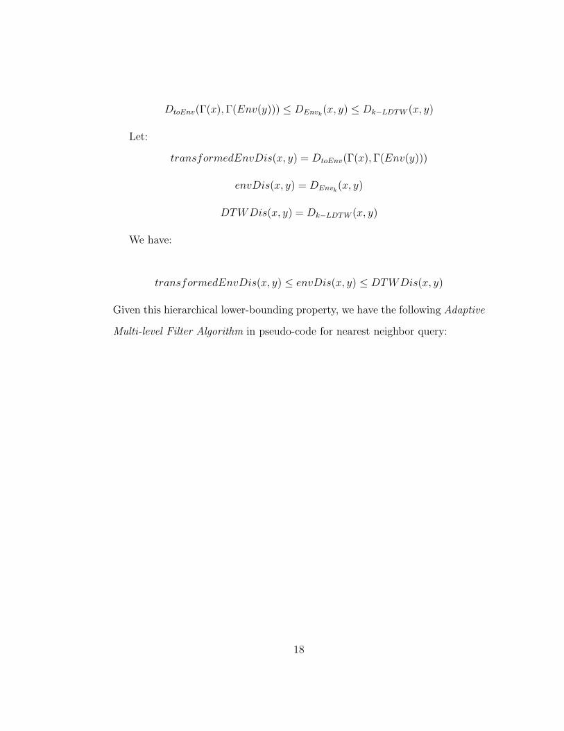
DtoEnv(Γ(x), Γ(Env(y))) ≤ DEnvk(x, y) ≤ Dk−LDTW (x, y)
Let:
transformedEnvDis(x, y) = DtoEnv(Γ(x), Γ(Env(y)))
envDis(x, y) = DEnvk(x, y)
DTWDis(x, y) = Dk−LDTW (x, y)
We have:
transformedEnvDis(x, y) ≤ envDis(x, y) ≤ DTWDis(x, y)
Given this hierarchical lower-bounding property, we have the following Adaptive
Multi-level Filter Algorithm in pseudo-code for nearest neighbor query:
18

Given a query time series q
1 //set minimum distance to infinity
2 minDis=infinity
3 for all candidates x in database
4 { disLevelOne = transformedEnvDis(q,x)
5 //transformed envelope filter check
6 if (disLevelOne < minDis)
7 { disLevelTwo = envDis(q,x)
8 //envelope filter check
9 if (disLevelTwo < minDis)
10 { disLastLevel = DTWDis(q,x)
11 //true DTW distance check
12 if (disLastLevel < minDis)
13 { //found a better match
14 bestMatch = x
15 //update the minimum distance
16 minDis = disLastLevel
17 }//if at last level
18 }//if at level two
19 }//if at level one
20 }//for
This algorithm guarantees no false negatives and can be easily modified to
handle k-nearest neighbor query.
19

2.4.4 Piecewise Aggregate Approximation Based Trans-
formation
The envelope transformation which was constructed based on Piecewise Ag-
gregate Approximation (PAA) has proven to be a good transformation for the
multi-level filter Algorithm [37]. The following gives its definition.
• Piecewise Aggregate Approximation (PAA)
5 KAIS Long paper submitted 5/16/00
3. Piecewise Aggregate Approximation
3.1 Dimensionality reduction
We denote a time series query as X = x1,…,xn, and the set of time series which constitute thedatabase as Y = {Y1,…YK}. Without loss of generality, we assume each sequence in Y is n unitslong. Let N be the dimensionality of the transformed space we wish to index (1 ≤ N ≤ n). Forconvenience, we assume that N is a factor of n. This is not a requirement of our approach,however it does simplify notation.
A time series X of length n is represented in N space by a vector NxxX ,,1= . The ith elementof X is calculated by the following equation:
∑+−=
=i
ijjn
Ni
Nn
Nn
xx1)1(
(3)
Simply stated, to reduce the data from n dimensions to N dimensions, the data is divided into Nequi-sized "frames". The mean value of the data falling within a frame is calculated and a vectorof these values becomes the data reduced representation. Figure 2 illustrates this notation. Thecomplicated subscripting in Eq. 3 is just to insure that the original sequence is divided into thecorrect number and size of frames.
Figure 2: An illustration of the data reduction technique utilized in this paper. A time series consisting ofeight (n) points is projected into two (N) dimensions. The time series is divided into two (N) frames and themean of each frame is calculated. A vector of these means becomes the data reduced representation.
Two special cases worth noting are whenN = n the transformed representation isidentical to the original representation. WhenN = 1 the transformed representation issimply the mean of the original sequence.More generally the transformation producesa piecewise constant approximation of theoriginal sequence, we therefore call ourapproach Piecewise AggregateApproximation (PAA).
In order to facilitate comparison of PAAwith the other dimensionality reductiontechniques it is useful to visualize it asapproximating a sequence with a linearcombination of "box" basis functions. Figure3 illustrates this idea.
The time complexity for building theindex for the subsequence matching problemappears to be O(nm), because forapproximately m "windows" we mustcalculate Eq. 3 N times, and Eq. 3 has a
0 1 2 3 4 5 6 7 8 9-2
-1
0
1
2
X = (-1, -2, -1, 0, 2, 1, 1, 0) n = |X| = 8
X = (mean(-1,-2,-1,0), mean(2,1,1,0) ) N = | X | = 2
X = ( -1 , 1)
Figure 3: For comparison purposes it is convenient to regardthe PAA transformation X’, as approximating a sequence Xwith a linear combination of "box" basis functions
0 20 40 60 80 100 120 140
x0
x1
x2
x3
x4
x5
x6
x7
X
X’
Figure 2.7: The PAA transformation (figure from [16])
PAA was proposed independently by B. K. Yi and C. Faloutsos [33] and
E. Keogh, K. Chakrabarti, M. Pazzani and S. Mehrotra [16]. It is a data
reduction method which divides a time series of length n into N segments
of equal length, see Figure 2.7.
A time series x of length n can be approximated in N space by a vector
X = X1, X2, . . . , XN :
Xi =N
n
b n
N∗ic
∑
j=b n
N∗(i−1)c+1
xj (2.7)
20

where bxc is called the floor function which returns the maximum integer
that is not greater than x.
The time complexity is O(N + n) = O(n) [16].
• PAA Envelope Transformation
The PAA envelope transformation is constructed as follows:
Ei =N
n
b n
N∗ic
∑
j=b n
N∗(i−1)c+1
xj , Ei =N
n
b n
N∗ic
∑
j=b n
N∗(i−1)c+1
xj (2.8)
It can be proven that the PAA envelope transformation is container invari-
ant. Suppose that there is a time series y = y1, y2, ..., yn and an envelope
time series Env(x) = (x, x) and y ∈ Env(x), we know xj ≤ yj ≤ xj for
all j = 1, 2, ..., n
Consider applying the PAA transformation on y and the PAA envelope
transformation on Env(x), then for i = 1, 2, ..., N ,
Ei =N
n
b n
N∗ic
∑
j=b n
N∗(i−1)c+1
xj ≤N
n
b n
N∗ic
∑
j=b n
N∗(i−1)c+1
yj = Γ(y)i
Similarly Γ(y)j ≤ Ej. So Γ(y) ∈ Γ(Env(x)). Therefore, the PAA transfor-
mation is container invariant and the PAA transformed envelope distance
lower-bounds the envelope distance.
2.5 Data Preparation
In most cases, a good similarity measure allows various distortions of the time
series. Otherwise the time series need to be normalized before the actual sim-
21

ilarity measure. The following is a list of distortions and the corresponding
solutions to eliminate the distortions.
• Amplitude Shifting Distortion:
An (amplitude) shifting by δ on a time series x = (x1, x2, ..., xn) is
Shift(x, δ) = x + δ = (x1 + δ, x2 + δ, ..., xn + δ).
This distortion can be eliminated by subtracting the average of each time
series from the values in the time series. In this way, every time series
is normalized to have an average 0. Let δ = avg(x) =∑n
i=1 xi, the time
series x after normalization is Shift(x,−δ).
• Amplitude Scaling Distortion:
An (amplitude) scaling by β on a time series x = (x1, x2, ..., xn) is
Scale(x, β) = βx = (βx1, βx2, ..., βxn).
This distortion can be eliminated by first subtracting the average value
and then dividing by the resultant time series’s standard deviation. In
this way, every time series is normalized to have the average 0 and the
same standard deviation value 1. Let β = std(x) =√
∑ni=1(xi − avg(x))2
; the time series x after normalization is Scale(Shift(x − avg(x)), 1/β).
• Global Time Scaling Distortion:
A global time scaling on a time series uniformly squeezes or stretches the
time series on the time axis.
A w-up-scaling of a time series x of length n is Uw(x) = y of length nw,
where yi = xbi/wc, i = 0, 1, ..., nw − 1;
22

A w-down-scaling of a time series x of length n is Dw(x) = z of length
bn/wc, where zi = xiw, i = 0, 1, ..., bn/wc − 1.
This distortion can be eliminated by up-scaling or down-scaling each time
series to a uniform length.
• Global Time Shifting Distortion:
A global time shifting by i (which can be negative) on a time series x =
(x1, x2, ..., xn) is TShift(x, i) = (x′1, x
′2, ..., x
′n), where x′
j = xj+i for 0 <
j ≤ n and xj+i = x1 if j + i < 1(when i is negative) and xj+i = xn if
j + i > n(when i is positive).
This distortion, also called lag, can be detected and eliminated by applying
a lagged distance measure or a time warping distance measure, which
allows for extra or missing elements at the beginning or end.
• Local Time Shifting Distortion:
For local time shifting, the shifting happens locally and non-uniformly.
This distortion can be solved by applying a distance measure that allows
time warping.
• Background Noise:
Sometimes the query or data contains unavoidable random noise data.
This noise is comparable to the low-pitch or high-pitch background noise
in a recording or the disturbance in a radio broadcast.
This noise can be removed by applying signal processing techniques such
as low- or high-band-filtering.
23

For more detailed information about related work on time series matching,
see D. Gunopulos and G. Das[12] and Keogh [13]; both gave a tutorial on
time series similarity search which covered the topics of similarity measures and
indexing. Shasha and Zhu’s book [28] is also a valuable tutorial on time series
techniques with case studies.
2.6 Summary
This chapter reviewed a few important techniques related to time series match-
ing: the GEMINI framework, the DTW and related indexing techniques such
as the envelope filter and the tranformed envelope filter. The next chapter will
present our time series matching framework.
24

Chapter 3
Time Series Matching
Framework
Here we present our time series matching framework. It is a framework to easily
optimize, combine and test different features to perform fast similarity searches
based on the application requirements. The framework can be easily extended
and it provides a collection of simple and easy-to-use tools. For example, there
is a tool analyze feature measure and generate distribution charts; there is a
tool to combine a few feature measures into a feature measure; there is tool to
generate algorithm which is written tersely in the configuration file.
We will first formalize the problem, then present the functionality and struc-
ture of the framework and finally give explanatory examples. In the following
we discuss time series, but the framework works on any ordered array data.
25

3.1 Formal Problem Statement
Our goal is to build a time series matching algorithm which can be customized
for any application. It can be formalized as follows:
Given any training data for an application, there is a set of time series data
pairs:
S = {(q1, r1), (q2, r2), ...(qn, rn)}
where
• Each ri = {ri(0), ri(1), . . . , ri(li)} is a time series reference data of some
finite length li; r = ∪ri for i = 1, 2, . . . n,
• Each qi = {qi(0), qi(1), . . . , qi(hi)} is a time series query data of some finite
length hi; q = ∪qi for i = 1, 2, . . . n,
• The ri is considered the best match to qi
Let us say that for each query q there is a function correctmatch such that
correctmatch(q) is the best match for q in the database. (The criterion for
“best” depends on the application, e.g. the song the most closely corresponds
to a humming as far as the user is concerned.) Here we assume all the correct
match ri for qi are in the database.
If G is an algorithm for matching and we have a threshold k, then G(qi) =
p1, p2, ..., pk. We say G is correct on qi if ri belongs to G(qi). We want to find
the G that maximize the number of qi for which G is correct.
26

All
Candidates
Fewer
CandidatesFewer
Filter
1
Filter
2
Query Data
Final
CandidatesFinal
Filter
Figure 3.1: Multi-filter algorithm structure
3.2 Framework Overview
Given any application training data, the framework can be used to build a
multi-filter algorithm as shown in Figure 3.1. At each filter level, the algorithm
compares certain features of the query and reference data and filters out bad
candidates; the number of candidates becomes smaller and smaller; finally the
algorithm gets a list of candidates which are similar to the query data. The last
filter will rank the results.
A filter can be very simple and compare only a simple feature of the query
and candidates; or it can be very complicated and by itself be a ranking algo-
rithm; or it can be a boosted set of filters. We will discuss Boosted Filters in
27

detail later in the thesis.
Unlike the GEMINI framework where the similarity measure is defined be-
forehand, the framework “learns” the best similarity measure on the training
data. The best similarity measure with the correct goal is not explicitly defined
before training and it may not match all the query data to the correct reference
data. Thus it is hard to define “guarantee no false negatives”. Each filter simply
maximizes the correctness of the labeling on good candidates.
3.3 Functionalities
The major functionalities of the framework are analyzing features, building
matching algorithms, boosting filters, benchmarking and validating algorithms.
3.3.1 Feature Analysis
The framework helps analyze any specific feature of the time series data. Tech-
nically, it is analyzing different feature parameters or comparison methods for
any particular feature. The user defines how to compute a particular feature
and how to compare two feature values; the framework automatically computes
the features for all the training data, compares them and outputs an analysis;
based on the analysis, the user can decide whether or not, and how, to use the
feature to build a filter in the algorithm.
3.3.2 Building an Algorithm
The framework can be used to build a similarity matching algorithm. The user
simply defines the filters in a text configuration file. Each filter is a line of text
28

which consists of the name of the feature comparison function and the condition
test. The framework will read the configuration file and dynamically generate a
multi-filter algorithm for the similarity measure. The order of the filters in the
text file is the order of the filters in the algorithm.
The filters to be used in the algorithm are selected based on both the feature
analysis and on the benchmark results. The configuration for building the
algorithm can be easily altered to change the order and the parameters of each
filter.
In some cases, a simple filter may not work well, such as when it has a high
percentage of false negatives . Then a more sophisticated filter should be used,
such as boosted filters as described next.
3.3.3 Boosted Filters
Boosting [11, 26, 25] is an algorithm for constructing a ‘stronger’ classifier using
only a training set and a set of ‘weak’ classifiers. We can use it to combine
simple filters into a more discriminating filter.
Figure 3.2 is an example of simple boosting. W1, W2, W3 are three weak
classifiers, each of which has above 50% but much less than 100% probability to
correctly classify a datum. Each datum can be classified as one of two classes:
black or white.
Suppose A, B, C are three data each respectively belonging to the class black,
white and black. W1 will label A, B, C as black, white and white respectively;
W2 will label A, B, C as all black; W3 will label A, B, C as white, white and
black respectively. We can construct a stronger classifier S which is a linear
combination of W1, W2, W3. By assigning appropriate weights to W1, W2, W3
29

TrainingData
W1 W2 W3 S
1/3 1/3 1/3
+ +
A
B
C
D
Figure 3.2: Ada boosting
(1/3 each), S will treat A as 13
black + 13black + 1
3white, and by rounding it to
the majority decision, it will correctly classify A as black. Also, S will correctly
classify B and C. The probability to correctly classify a datum for S is 100%.
As proven in [11], for reasonable distributions, for any other datum D, it is
highly likely that S will classify it correctly. The process of computing the
appropriate weights for weak classifiers is called boosting.
Our framework is using a specific version of the boosting algorithm called
AdaBoost.MR: a multiclass, multi-label version of AdaBoost based on ranking
loss. More details can be found in Appendix A.
It is suggested in [29] that the decision tree algorithm is a good algorithm
30

to detect weak classifiers as good candidates for boosting [26]. So the framework
also supplies a tool to build decision trees.
3.3.4 Algorithm Assessment
Benchmark
Once an algorithm is built, the framework can be used to benchmark and val-
idate the algorithm. By selecting different testing data sets, the benchmark
result will show whether the algorithm is general enough to cover not only the
training data but also the testing data.
Cross-validation
The simplest and most widely used method for estimating prediction error is
k-fold cross-validation [30]. Basically, given the training data, we randomly
divide them into k roughly equal-sized parts; picking the i-th part, we train the
algorithm with the other k − 1 parts and test the result on the i-th part; we
do this for each i in 1 . . . k. We usually choose 10 as k based on the general
observation that 10 is a good value.
If the training error and testing error do not change more than 5% as i
changes, it means that the algorithm is general enough with regards to the
data selection. If the testing error is much bigger than the training error, it
means that the algorithm has an overfitting problem, indicating that a different
parameter setting should be used.
The framework uses 10-fold cross-validation to assess the generality of the
parameters, such as the condition test value for the simple filters and the weights
for the boosting filters.
31

Scalability Test
By increasing the size of the reference database step by step, the framework can
assess the scalability of the algorithm it builds.
For each scale level of the reference database, we need to make sure the
prediction error estimate is accurate. So Bootstrapping [30] is used to make
sure the data selected for testing is general enough that our prediction error for
this scale level is reasonable.
Suppose:
• The scale we want to test is a reference database R′ of m time series;
• The whole reference data space is R of size n (m < n);
• The current testing data are k (k < m) pair of time series
S = {(q1, r1), (q2, r2), ...(qk, rk)}
and
RT = ∪ri, RT ⊂ R for i = 1, 2, . . . k
where
1. the ri is considered the best match to qi.
Bootstrapping:
For about C = 1000 times (a customary number),
• Select m−k time series data uniformly with replacements from R to form
a set RS;
32

• Use R′ = RT ∪ RS as a benchmark reference database and compute the
prediction error
Output the C prediction errors and the average prediction error.
If the C prediction errors have low standard deviation, then the algorithm
does not depend much on the selection of data. The average prediction error
gives a good idea of what the prediction error is in the general case.
3.4 Framework Components
3.4.1 Overview
The framework consists of the following major components from bottom to top:
• Transformation Functions
• Comparison Functions
• Features
• Feature Measures
• Conditions
• Filters
• Algorithms
The relationship between the different components is shown in Figure 3.3.
A more detailed explanation can be found in the following subsections.
33

Time series data
features
Features: envelope time series,
time series, scalar data
feature measures
filters
transforms
transforms
+ comparison functions
+ condition check
+ order and boost function
algorithms
Figure 3.3: Framework components from bottom to top
3.4.2 Transformation Functions
Transformation functions are primitive functions that transform data from one
form to another, such as the Discrete Fourier Transform (DFT) [28] that trans-
forms data from the time domain to the frequency domain.
Currently there are three data forms in the framework: scalar, time series
and envelope time series.
• Scalar
A single real value.
• Time Series
A real value sequence with finite length.
34

• Envelope Time Series
A set of two finite length real number value sequences. In the case that
each element’s value in the first number sequence is greater than the corre-
sponding element in the second number sequence, we call the first number
sequence a higher envelope and the other a lower envelope.
3.4.3 Comparison Functions
Comparison functions are functions that compare two data items and return a
scalar value. The scalar value is 0 when two data are considered equal. It can
be negative; a positive value means the first datum is “bigger” in the measure’s
sense and a negative value means the first datum is smaller.
The comparison function is often reflexive and symmetric. It might either
be transitive or satisfy the triangle inequality. Currenly we don’t make use of
these properties. But they can served as meta information in case we want to
automate the framework process in the future. The two data items could be of
the same or of different form; the restriction on the function is very loose. The
maintainer of the framework needs to understand the functions to use them.
Suppose F is the comparison function and q, r are two data inputs. It may
satisfy the following properties. These properties may be used to automate the
process to create new feature measures.
• Reflexive
F (q, q) = 0
This property does not usually hold when F applies only to two data of
different forms with a special order such as envelope distance measure.
35

• Symmetric (on absolute value)
|F (q, r)| = |F (r, q)|
under the condition that F (q, r),F (r, q) can be computed.
This property does not usually hold when F only applies to two data of
different forms with a special order such as envelope distance.
• Transitive
F (q, r2) = F (q, r1) + F (r1, r2)
when q, r1, r2 are of the same data form and F (q, r) could return a negative
value.
This property does not usually hold when F only applies to two data
of different forms with a special order such as dynamic warping distance
measure.
• Triangle Inequality (on absolute value)
|F (q, r2)| ≤ |F (q, r1)| + |F (r1, r2)|
when q, r1, r2 are of the same data form and F (q, r) returns a negative
value.
3.4.4 Features
Transformation functions compute feature data from the original time series
data or other feature data, as in Figure 3.1.
36

3.4.5 Feature Measures
The comparison functions, together with the feature data, comprise feature
measures, as in Figure 3.1. A comparison function can apply to different feature
data to construct different feature measures.
3.4.6 Conditions
The condition functions, together with the feature measures, construct filters.
A feature measure having different condition thresholds forms different filters,
one for each threshold.
3.4.7 Filters
As we mentioned earlier, we built a multi-filter algorithm based on the filters.
At each filter level, the algorithm uses one or more feature measures to com-
pare certain features of the query and reference data and filters out some bad
reference candidates.
Consider a classifier which labels each candidate ‘good’ or ‘bad’. If it always
gives the correct answer, it is considered a perfect classifier which can be directly
used as one filter in the multi-filter chain; if it gives the correct answer much
more than 50% of the time, it is called a strong classifier; if it gives the correct
answer slightly more than 50% of the time, then it is called a weak classifier,
which can be combined with other weak classifiers to create a boosted strong
classifier. Each filter in the multi-filter chain of the algorithm should be at least
a strong classifier if not a perfect classifer.
37

3.5 Component Examples
In this chapter we will show how easy it is to create components with K[1] ex-
ample codes. A long list of the example framework components are in Appendix
B. Here we present only a few examples, which will be helpful in understanding
Section 3.6.
3.5.1 Example Transformation Functions
Each transformation function component has 3 APIs: name, description and
compute, where the API function compute is required and the other two are
helpers for the purpose of debugging or display.
For K[1] code implementation, each transformation function has an entry in
the dictionary .transform.
• Remove Average(deavg):
Subtract the average value from each element in the time series.
K code:
\d .transform.deavg
name:”Subtract the Average”
description:”Subtract the average value from each element
in the time series”
compute:{[x] :x-(+/x)%x}
• Zero Crossing Rate(zcr):
Compute how many times the time series data cross the average line.
38

K code:
\d .transform.zcr
name:”Zero Crossing Rate”
description:”Compute how many times the time series cross
the average line”
compute:{[x] x:.transform.deavg.compute[x]
/rest of the implementation omitted}
This transformation reuses the deavg tranformation to preprocess input
data.
• Direction Change Count(dcc):
Compute how many times the time series data changes direction, either
up or down.
K code:
\d .transform.dcc
name:”Direction Change Count”
description:”Compute how many times the time series data
changes up or down direction”
compute:{[x] /implementation omitted}
3.5.2 Example Comparison Functions
Each comparison function component has 3 APIs: name, description, com-
pare, where the API function compare is required and the other two are
39

helpers for the purpose of debugging or display. API compare takes two values
as input. The forms of the two input values may be different and the order of
input usually matters.
For the K[1] code implementation, each comparison function has an entry
in the dictionary .measure.
• Subtraction(subtraction)
C(q, r) = r− q, where q, r are both scalars or both time series of the same
length.
It is reflexive, symmetric on absolute value and transitive. It satisfies the
triangle inequality on absolute value when both input are scalars.
K code:
\d .measure.subtraction
name: ”subtraction”
description: ”Subtraction of the first datum from the second”
input: ‘ts
compare:{[q;r]:r-q}
/note that the order of the subtraction is important
• α%-Local Dynamic Time Warping(ldtw)
It computes the k-local dynamic time warping distance between two time
series q, r where k = 1 + n ∗ α% and n is the length of q. It is reflexive.
40

3.5.3 Example Feature
Each feature component has 4 APIs: name, description, input and com-
pute where the API functions input and compute are required and the other
two are helpers for the purpose of debugging or display.
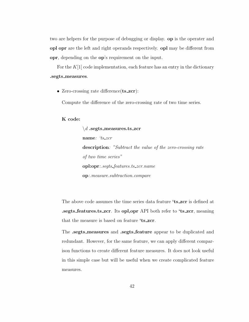
For the K[1] code implementation, each feature has an entry in the dictionary
.segts features.
• Relative offset of the time series(ts rel):
For each consecutive pair in the time series, subtract the two values in the
pair and we get a new time series.
K code:
\d .segts features.ts rel
name: ‘ts rel
description: ”Relative offset of the time series”
input: ‘ts
compute: {[x]:-’:x}
The above code assumes the time series data feature ‘ts is defined at
.segts features.ts. Its input API refers to ‘ts, meaning that the feature
‘ts rel can be computed from feature ‘ts using its compute API.
3.5.4 Example Feature Measures
Each feature measure component has 5 APIs: name, description, opl, opr
and op, where the API functions opl, opr and op are required and the other
41
two are helpers for the purpose of debugging or display. op is the operater and
opl opr are the left and right operands respectively. opl may be different from
opr, depending on the op’s requirement on the input.
For the K[1] code implementation, each feature has an entry in the dictionary
.segts measures.
• Zero-crossing rate difference(ts zcr):
Compute the difference of the zero-crossing rate of two time series.
K code:
\d .segts measures.ts zcr
name: ‘ts zcr
description: ”Subtract the value of the zero-crossing rate
of two time series”
opl:opr:.segts features.ts zcr.name
op:.measure.subtraction.compare
The above code assumes the time series data feature ‘ts zcr is defined at
.segts features.ts zcr. Its opl,opr API both refer to ‘ts zcr, meaning
that the measure is based on feature ‘ts zcr.
The .segts measures and .segts feature appear to be duplicated and
redundant. However, for the same feature, we can apply different compar-
ison functions to create different feature measures. It does not look useful
in this simple case but will be useful when we create complicated feature
measures.
42

More importantly, the result of a feature measure is a monotonic scalar
value which we can analyze and determine a parameter to create filters.
In a way similar to creating the feature measure .segts measures.ts zcr,
we can create the feature measure .segts measures.ts dcc using feature
.segts features.ts dcc and comparison function .measure.subtraction.
We will compare these two feature measures ts zcr, ts dcc later in section
3.6.
3.5.5 Example Conditions
The condition keywords are used in the algorithm builder configuration file to
create filters. Some examples are as follows.
• e: Feature value is equal
• le: Measure value equal to or less than
• ge: Measure value equal to or greater than
• in: Measure value is in a range
• rank: Rank of measure value among all reference data in DB
3.5.6 Example Filters
We will show how easy it is to use a configuration file to prototype algorithm
and how easy to make changes to an algorithm.
Each line in the algorithm builder configuration file defines a filter. The
format is ’condition, feature measure, condition value’. To add a new filter,
simply add a new line; to remove a filter, simply remove or comment out the line.
43

The framework can load the new configuration file and generate the algorithm
for matching. Each algorithm can be stored in a separate terse text file which
makes it very easy to maintain.
For example, suppose the query datum is q, a reference datum is r, and M
is a feature measure for q, r.
• e,ts zcr,1
M(q, r) = ts zcr(r, q) =
1 if (rts zcr == qts zcr)
0 otherwise
where rts zcr and qts zcr are the ts zcr feature of q and r respectively.
This filter will consider r as a good candidate only if
M(q, r) == 1
In this example, the feature measure ts zcr incidentally has the same
name as the feature name ts zcr it used to test the condition.
• le,ts dcc,3
M(q, r) = ts dcc(r, q) = rts dcc − qts dcc
where rts dcc and qts dcc are the ts dcc feature of q and r respectively.
Since we specify the threshold as 3, this filter will consider r a good
candidate only if
M(q, r) ≤ 3
In this example, the feature measure ts dcc incidentally has the same name
as the feature name ts dcc it used to test the condition.
44

• rank,ts ldtw5,15
Here ts ldtw5 is the feature measure that computes the 5% local dynamic
time warping distance between the query datum and reference datum,
M(q, r) = ts ldtw5(r, q) = ldtw(q, r)
where the warping parameter α% is the default 5%.
This filter will consider r as a good candidate only if its 5% local dynamic
time warping distance to q is one of the 15 smallest values among all the
reference data’s 5% local dynamic time warping distances to q.
3.5.7 Example Boosted-Filter
In the algorithm builder configuration file, a boosted filter is represented as a
few text lines as follows:
1. The first line is “boost{ weights” where a “{” separates keyword“boost”
and the weights for the combining filters. The weights are a list of numbers
separated by “,”;
2. Each line of the following lines defines a filter as in Section 3.5.6. The i-th
filter’s weight is the i-th number in the number list;
3. The boosted filter ends with “}”.
Suppose the boosting algorithm suggests that three filters (e,ts zcr,1),
(le,ts dcc,3), (rank,ts ldtw5,15) can be combined with equal weights 0.33,
0.33, 0.33 to create a stronger filter. It can be represented as:
45

Config file text:
boost{1,1,1
e,ts zcr,1
le,ts dcc,3
rank,ts ldtw5,15
}
The weights in the example are 1,1,1 which will be automatically normalized.
3.6 Usage Examples
3.6.1 Feature Measure Analysis
The framework can generate a report for any distance feature measure M for
further analysis. This makes it convenient to analyze and experiment new fea-
ture measures.
For any training data S = {(q1, r1), (q2, r2), ...(qn, rn)} where ri is the correct
match for qi, M(qi, rj) will be computed for all i from 1 to n and all rj ∈ R.
We look at two distributions:
• The distribution of M(qi, ri) for all i, (P ):
It gives information about whether the M gives a distance value close to
zero for correct matches.
• The distribution of M(qi, rj) for a fixed i and all rj ∈ R, (Qi):
It gives information about whether the M can distinguish the correct
matches from the incorrect ones.
46

Situations:
• If M is consistantly low for correct matches and consistantly high for
incorrect ones, then M is a good feature measure.
• In other cases, M might be used as weak classifier. Since a weak classifier
only needs to have slightly higher than 50% correctness probability, if it
is worse than 50% probability, then the reverse would be a weak classi-
fier. The only case where a measure is useless is when the correctness
probability is 50%.
For example, usually Direction Change Count is not a good feature mea-
sure for data with even small noise.
Considering a time series datum 1, 2, 2, 2, 1 as the reference data, the
direction change count is 1. If there is some noise in the query data, say 1.0,
2.0, 1.9, 2.0, 1.0, the direction change count in the query data is 3!
3.7 Summary
This chapter explained the structure and functions of the time series matching
framework. Given any application training data, the framework can be used
to build a multi-filter algorithm to perform an accurate and efficient similarity
search. In the next chapter, we will study a case of a music retrieval system. We
will apply this time series matching framework to analyze music data and build
a similarity search algorithm to match people’s humming to music melodies.
47

Chapter 4
Case Study: Query-by-humming
A Query by Humming (QbH) system allows the user to find a song by humming
part of the tune. The idea is simple: the user hums into the microphone;
the computer records the humming and extracts certain melody and rhythm
features; then it compares these features to those of the songs in the database;
finally it returns a ranked list of the songs or song segments most similar to
the humming. There are several applications for this technology, such as music
search engines, cell phone ring-tone searches, karaoke scoring and music learning
software.
Usually the evaluation of a query-by-humming system is based on human
judgment. We say a hummed tune is human recognizable if any person who
knows the song being hummed can recognize the song from the humming. We
say a hummed tune is top-K system recognizable if the song name is in the
system’s top K list (K is usually small, 1, 5 or 10). Given a set of hummed
tunes, the percentage of hummed tunes that are recognizable by the system is
called the hit rate. The higher the hit rate, the higher the accuracy.
48

TopKhitrate =the number of TopK system recognizable
the number of human recognizable
My goal is to build a fast and accurate system with thousands and eventually
millions of songs. I will first compare related work on QbH systems, then pro-
pose an approach to improve one of them, and finally show some experimental
results.
4.1 Related Work Review
Currently there are several Query-by-Humming systems being built and various
techniques have been applied.
1. String-represented note sequence matching
Alexandra Uitdenboderd and Justin Zobel [31] at RMIT University used
strings to represent the note sequence of music so that many fast and ma-
ture string-matching algorithms could be directly used. For example, each
interval between two notes is represented as a letter ”S” if the interval is
close to 0. However, it is very hard for a human to hum exact music notes;
so humming cannot be represented accurately by symbolic sequences of
music notes. As a result the accuracy of the system is not satisfactory.
The New Zealand Digital Library MELody inDEX developed by Rodger
J. McNab, Lloyd A. Smith, David Bainbridge and Ian H. Witten [21]
also used stringsa to represent music. They applied an approximate
string matching technique which is basically Dynamic Time Warped string
matching. As a result, the extended time taken to perform the approxi-
mate matching in large databases was still a problem. “The system con-
49

tains 9,400 folk songs and a 20-note search pattern requires approximately
21 seconds.” The bigger problem is that the returned list contains too
many entries and does not have a high top-K hit-rate for small K. An
online version of the system recently become available [2].
W. Archer’s [4] string editing matching algorithm is another variant of
the DTW string matching technique which allows missing of notes in the
humming.
Another novel idea is to not only dynamically match note values but also
dynamically match duration values.
2. Time Normalization and Partial Tone Transition
N. Kosugi, Y. Nishihara, T. Sakata, M. Yamamuro and K. Kushima’s
Large Music Database [19] “holds over 10,000 songs but the retrieval time
is about one second. And it is able to recognize the song and rank it
within the first 5 places on the list for about 70% of hummed tunes that
are recognizable to human beings as a part of a song”. Although this
performance is far from perfect, it is very good considering the scale of
the system. Also, it is a system that supports sub-sequence matching.
However, the system requires the user to hum with the syllable ‘ta’ and
requires the user to hum following the beats of a metronome.
Their system uses the music notes information from MIDI files. The dura-
tion of the notes in a song are normalized based on the most frequent du-
ration among all the notes. Then the song is segmented into subsequences
with equal duration lengths. The subsequence may be segmented into
subsubsequence if the most frequent duration among the notes in the sub-
50

sequence is smaller than the one among all the song notes; the subsequence
may be merged if the most frequent duration is bigger. Then the tone-
transition (relative note offset) feature is computed for each subsequence.
The partial tone-transition feature are extracted from the tone-transition
starting from a high note in the subsequence. Then the features are used
to compare query and reference candidates. Some indexing techniques are
used to speed up the system.
3. Melody slope matching
Y. Zhu, M. S. Kankanhalli and C. Xu [35] matched music based on the
music’s melody slope. For example, several adjacent notes are approxi-
mated by a line and the slope of the line will be treated as a feature. This
method is not equipped to handle a bad humming query, and thus will
not have high accuracy. However, this method may be used as one filter
to quickly remove bad candidates.
4. Dynamic Time Warping (DTW) on pitch contour time series
D. Mazzoni and R. B. Dannenberg [20] proposed a subsequence matching
algorithm which uses local time-warped distance measure to match music.
Although the precision is better than Euclidean distance, the response
time is not ideal because no indexing on DTW distance is applied.
Y. Zhu, D. Shasha and X. Zhao [37] used DTW distance measure and
the GEMINI framework with PAA-based envelope transforms. The songs
in the database were chopped into song segments based on melody and
transcribed into pitch contour. The query is compared to each song seg-
ment in the system using the adaptive multi-level filter algorithm. Both
51

the efficiency and precision results are very good on a small demo system
with 53 Beatles songs.
5. Survey
The survey paper on audio fingerprinting by Pedro Cano, Eloi Batlle, Ton
Kalker and Jaap Haitsma [6] is a significant paper on audio retrieval-by-
content algorithms. It gives a general framework with a list of algorithm
design requirements and a long list of algorithms. It also discusses different
distance metrics and different indexing methods.
Conclusion
From the survey and our experimental results, we can summarize the related
work as follows:
1. Warped distance is more robust
Generally, similarity measures that allow time warping have higher accu-
racy than those which use Euclidean distance or exact string matching.
2. Need to scale up
The computational complexity of time-warped matching is still prohibitive.
A real large scale system with millions of songs needs a better indexing
method and a more discriminative similarity measure.
3. Difficulty of performance comparison
Although there are successful works on query-by-humming systems, it is
hard to compare the results for the following reasons:
• No standard for evaluation
52

(a) The data set and testing set are different.
The music collection and the size of the database varies greatly.
The testing sets are generally too small to be statistically mean-
ingful. Also, the selection of the testing will affect the result. For
example, some melodies are more distinguishable than others.
(b) The definition of accuracy is not reliable
The hit-rate definition is based on human’s recognition of hum-
ming, which is not reliable. For example, a human can recog-
nize a hummed tune by recognizing the most distinguishable part
even if other parts may be out of tune. Also, a human who knows
only a few songs might more easily recognize more hummed tunes
than a human who knows a lot of songs, who may not recognize
a hummed tune because it is similar to many tunes. So a human
may mistakenly label a hummed tune because of their personal
knowledge.
• No easy access to the system
Only two of above systems have online interfaces, one of which was
not accessible until very recently.
Since I am continuing my work based on Yunyue Zhu’s system [37], I will
use that system as a benchmark reference. The evalution process is to first
have more than 3 people verify each humming. Only hummings that can be
recognized by at least 3 people are used for the system training. Also, the
reference database for training contains only songs of the training hummings to
avoid influence of other song data.
53

4.2 Our Query-by-humming System
Our system uses the time series matching framework to learn the measure in-
stead of relying purely on a single distance measure.
4.2.1 New Workflow
The workflow of the new system is an extension of the old system from [37], see
Figure 4.1. We will first give a query work flow example here and then discuss
the key ideas in detail.
note/durationsequence
segmentnotes
Query criteria
Database
Humming with ‘ta’
keywords
Top Nmatch
Nearest-Nsearch
on DTWdistancewith transformedenvelope filter
melody (note)
TopN’
match
Alignment
verifier
rhythm (duration)& melody (note)
Database
statisticsbasedfeatures
Boostedfeature
filter
boosting
Database
Keyword
filter
Figure 4.1: New Query-by-humming System
Given a query,
1. Preprocessing
54

The humming is transcribed into pitch contours and extracted as a note
value sequence and duration value sequence.
2. Keyword filter
The candidate set is first filtered using the keyword if any keyword is
supplied.
3. Multiple Statistical Feature Filters
The candidate set is further filtered based on a multi-filter chain, some of
which are boosted filters.
4. Adaptive multi-level DTW filters
The melody (note-sequence) information is used as a query to obtain a
top-K list. This step uses the same adaptive multi-level filter algorithm
as Yunyue Zhu’s framework except that note-sequences are used instead
of pitch-contours.
5. Alignment verifiers
For each candidate in the top-K list, the alignment between it and the
query is verified based on both the melody (note-sequence) and rhythm
(duration-sequence) information.
4.2.2 Key Idea: ‘ta’-based humming
Kosugi et al [19] showed that humming with only the syllable ‘ta’ can be easily
segmented into note-sequences; experiments also show the same result. Figure
4.2 shows two hummings of the same song segment. Unlike humming using ‘la’,
55

Figure 4.2: Compare humming using ‘ta’ and ‘la’
the humming using ‘ta’ has obvious rests between music notes which may be
because of the hard, short sound ‘t’.
By using ‘ta’-based humming, we can reduce the length of the time series
by orders of magnitude (from hundreds to less than 30). Then we can still use
DTW distance measure to compute the similarity. This preserves the flexibility
of warping while reducing the computational complexity.
The difference between our system and Kosugi’s system is that we don’t
require the user to hum with the aid of a metronome because a metronome is
usually not available and that requirement is not natural for a common user.
56
4.2.3 Key Idea: Low-Computation-Cost Filters
If a (boosted) filter has a lower computation cost than the DTW distance mea-
sure, then the system can use it as a filter to quickly weed out bad candidates,
thus improving the speed of the system. Many statistical feature measures, if
we set the condition loosely, can yield good filters.
Some features that the new framework currently uses to build filters are:
standard deviation of note value, zero crossing rate of note value, number of
local minima/maxima of note value, and a histogram of notes.
For example, based on the feature analysis, if the standard deviation of
the query note-sequence’s note value is 3.0, a standard-deviation-based weak
classifier may be defined as follows: any candidate whose standard deviation is
not between 1.5 and 4.5 is labeled “not similar” to the query.
Also, many statistical features are weak classifiers and usually computation
is fast. They can be combined into a boosted strong classifier.
Note that although a boosted classifier does not guarantee no false negatives,
it gives a high probability guarantee if we set parameters appropriately.
4.2.4 Key Idea: Alignment Verifiers
Whenever we compute a minimum DTW distance between two time series, we
get a particular alignment between them. It is wise to verify the alignment.
If two time series align well to each other globally (have a low DTW distance)
but align badly locally (the aligned elements have huge distance), we should not
consider it a good match. Figure 4.3 is such an example, the two time series do
not match. They align well globally but align badly at the 12, 13, 14th elements.
The 13th element of the upper time series is aligned to the 12th element of the
57

-2
-1
0
1
2
3
4
5
1 2 3 4 5 6 7 8 9 10 11 12 13 14 15 16 17 18 19 20 21
Figure 4.3: Good global alignment, bad local alignment
lower time series; the 14th element of the upper time series is aligned to the
13th element of the lower time series.
In our framework, the DTW distance is computed based solely on the melody
information. It is also wise to verify that the alignment is a reasonable alignment
for rhythm. Note that we cannot verify the rhythm alignment unless we know
which notes in the query correspond to which notes in the reference because
of the possibile note add/delete error. Several consecutive notes in the query
may correspond to one note in the reference or vice versa. After we determine
the time alignment based on the DTW distance computation, we can verify the
rhythm alignment.
58
4.3 Building the algorithm
4.3.1 Order of filters
Since speed is an important concern, the initial filters in the multi-filters chain
are better if they have a low computation cost. Here we assume that all the
features for the reference and query data are pre-computed, so the computation
cost for a filter mostly depends on the comparison function.
If a filter is based on a lower computation cost comparison function than
other filters, then it should be used first in the filter chain; on the other hand, if
a filter can largely reduce the size of the reference database, thus reducing the
full-scan cost for the next level, it should be used first as long as its computation
cost is not too high. The trade-off depends on how much of the full scan cost
the filter can save in the next level and how much the filter will cost for the
current level.
In our experiments, a filter based on the number of musical notes can be com-
puted quickly and effectively reduces the reference database set of candidates.
Suppose the query has kq notes, this filter computes the reference candidate
melody’s music note number, say kr, if kq/kr is not in (1 − a, 1 + b) (a, b are
trained parameters with positive value), then the reference candidate is not a
match for the query with very high probability (99.9%), and the filter can usu-
ally reduce the reference database size by about 25%. So this filter is placed at
the beginning of the algorithm filter chain.
Some filters have dependence on other filters such that they must be placed
after those prerequisite filters. For example, the duration alignment verifier can
be placed only after the DTW algorithm determines the alignment of notes,
59

because comparing the duration size is meaningful only if they correspond to
the same note.
4.3.2 Feature Analysis and Selection
For each feature, we can create different feature measures using different com-
parison functions. Then we can analyze the output of the comparison function
between the query datum’s feature and other reference data’s feature, as de-
scribed in section 3.6.1. The analysis will also give insights about the errors
people tend to make when they hum.
1. Number of Notes: Subtraction vs. Ratio
In our system, the songs are segmented into melody phases so we know
exactly the number of notes in each melody phases. For the training data,
the analysis shows the distribution for all the differences of the number of
notes between all the training (qi, ri) pairs. For example, given a query
qi and its matching reference ri, suppose the note number of query qi
is len(qi) and the note number of ri is len(ri); the distribution of the
difference len(qi) − len(ri) over i is what we are analyzing. If we use
the difference between the query and reference data’s number of notes to
check whether the reference data is a possible good match for the query,
it would be a good estimate since the distribution is condensed around a
small region with only a few exceptions, as shown in Figure 4.4(a).
Using the ratio betwen the number of notes is more intuitive since the
note number can be very small or big but the number of notes people add
in the humming may be proportional to the length of the melody. Figure
4.4(b) shows the distribution of len(qi)/len(ri) − 1 for all i. Although
60

no_len
0.00%
20.00%
40.00%
60.00%
80.00%
100.00%
-18.00
-16.53
-15.07
-13.60
-12.13
-10.67-9.20-7.73-6.27-4.80-3.33-1.87-0.401.072.534.00
(a) Subtraction of number of notes
no_len_ratio
0.00%
20.00%
40.00%
60.00%
80.00%
100.00%
-0.75-0.67-0.60-0.52-0.44-0.37-0.29-0.21-0.14-0.060.020.090.170.250.320.40
(b) Ratio of number of notes
Figure 4.4: The distribution of the measures based on the number of notes
61

it is only a little more condensed than Figure 4.4(a), here training data
are mostly short queries. More longer queries in the training data should
show a bigger difference.
2. Note value sequence’s standard deviation: Subtraction vs. Ratio
For the same reason, we chose to use the ratio between the query and the
reference data’s standard deviation of note value sequence rather than the
difference as a feature measure to build a filter. See Figure 4.5 for the
distribution of the subtraction/ratio between queries and the matching
songs’ standard deviation of the note value sequence.
3. Direction change count vs. Zero-crossing-rate
In our experiments, we find that the direction change count is not a good
filter, as shown in Figure 4.6(a). Slight noise in the data sequence dra-
matically changes the direction change count feature as in the example
below, which we have already seen:
Consider a time series datum 1, 2, 2, 2, 1 as the reference data, its direction
change count is 1. If there is some noise in the query data, say 1.0, 2.0,
1.9, 2.0, 1.0, the direction change count in the query data is 3! Each data
distortion might introduce two new direction changes.
Zero-crossing-rate tends to be a better measure, however, it is not stable
either, see Figure 4.6(b). So we will use the zero-crossing-rate measure to
build one of the filters to be boosted.
4. Relative note offset vs. Note value
There have been arguments about whether or not people will change bases
while humming. If so, then the relative note offsets between consecutive
62

no_stddev
0.00%
20.00%
40.00%
60.00%
80.00%
100.00%
-2.23-2.02-1.82-1.61-1.40-1.20-0.99-0.78-0.58-0.37-0.160.040.250.460.660.87
(a) Subtraction based
no_stddev_ratio
0.00%
20.00%
40.00%
60.00%
80.00%
100.00%
-0.64-0.57-0.49-0.42-0.34-0.27-0.19-0.12-0.040.030.110.180.260.330.410.48
(b) Ratio based
Figure 4.5: The distribution of note values’ standard deviation
63

no_dcc
0.00%
20.00%
40.00%
60.00%
80.00%
100.00%
-12.00
-11.07
-10.13-9.20-8.27-7.33-6.40-5.47-4.53-3.60-2.67-1.73-0.800.131.072.00
(a) Ratio of Direction Change Count
no_zcr
0.00%
20.00%
40.00%
60.00%
80.00%
100.00%
-4.00
-3.47
-2.93
-2.40
-1.87
-1.33
-0.80
-0.270.270.801.331.872.402.933.474.00
(b) Ratio of Zero Crossing Rate
Figure 4.6: Compare the direction change count and zero-crossing rate
64

note pairs form a better representation of the humming; otherwise the
absolute note values relative to the average captures the more accurate
information. Here we analyze and compare different feature measures
based on both relative consecutive note offset sequences and absolute note
sequences.
For each feature measure related to the note value sequence, a similar
feature measure is built based on the relative note sequence. For example,
one feature measure compares the most significant value (biggest absolute
value) of the mean-removed note sequence of the query and the refer-
ence candidate. A similar feature measure compares the most significant
value of the relative consecutive note offsets sequence of the query and the
reference candidate.
The experimental results do not strongly favor one over the other in most
cases. If we use the most significant absolute value in the mean-removed
note sequence as a feature, the ratios between the query and reference
pairs have a distribution similar to that if we use the most significant
absolute value in the relative note offset sequence, as in Figure 4.7. In
our algorithm, we use the former feature to build one of the filters to be
boosted.
If a feature is based on the difference between the maximum and minimum
values in the note sequence, the ratios between the query and reference
pairs’ feature have a distribution slightly more condensed than that if we
use the most significant absolute value in the relative note offset sequence,
as in Figure 4.8. In our algorithm, we use the former feature to build one
of the filters to be boosted.
65

no_deavg_sig_ratio
0.00%
20.00%
40.00%
60.00%
80.00%
100.00%
-0.59-0.51-0.44-0.36-0.28-0.20-0.13-0.050.030.110.180.260.340.420.490.57
(a) For note sequence
no_rel_sig_ratio
0.00%
20.00%
40.00%
60.00%
80.00%
100.00%
-0.59-0.51-0.44-0.36-0.28-0.20-0.13-0.050.030.110.180.260.340.420.490.57
(b) For relative note offsets
Figure 4.7: The distribution of the ratio of most significant value
66

no_maxVSmin_ratio
0.00%
20.00%
40.00%
60.00%
80.00%
100.00%
-1.50-1.30-1.10-0.90-0.70-0.50-0.30-0.100.100.300.500.700.901.101.301.50
(a) For note sequence
no_rel_maxVSmin_ratio
0.00%
20.00%
40.00%
60.00%
80.00%
100.00%
-1.50-1.30-1.10-0.90-0.70-0.50-0.30-0.100.100.300.500.700.901.101.301.50
(b) For relative note offsets
Figure 4.8: The distribution of the max-min value difference
67

no_ldtw_no5
0.00%
20.00%
40.00%
60.00%
80.00%
100.00%
0.100.370.640.901.171.441.711.982.242.512.783.053.323.583.854.12
(a) For note sequence
no_ldtw_no_rel5
0.00%
20.00%
40.00%
60.00%
80.00%
100.00%
0.120.370.630.881.131.391.641.892.152.402.652.913.163.413.673.92
(b) For relative note offsets
Figure 4.9: The distribution of the LDTW measure on the first 5 values
68

If a feature is based on the local dynamic time warping (DTW) distance of
the first 5 elements’ values in the mean-removed note sequence, the ratios
between the query and reference pairs’ feature have a distribution that
is more condensed than that if we use the local dynamic time warping
distance of the first 5 elements in the relative note sequence, as in Figure
4.9. This is easily explained: if there is some note added into or deleted
from a few consecutive notes with similar values in the note sequence, the
relative note sequence would have errors that cannot be handled by the
dynamic time warping measure. For example, suppose the song melody is
55, 62, 62, 55, 58, . . . where the durations are 4, 1, 1, 4, 4, . . ., the query
may merge two short notes of value 62 into one longer note, such as 55, 62,
55, 58, . . .. The DTW distance measure will give a small distance between
the query and reference note sequence. But for the relative note sequence
feature, the query becomes 7, -7, 3, . . . and the reference becomes 7, 0,
-7, 3, . . . and the DTW distance measure will give a big distance between
them. In our algorithm, we use the local dynamic time warping distance
of the first 5 elements’ values in the mean-removed note sequence as a
feature to build one of the filters to be boosted. No duration information
is used though.
5. Which to use as measure reference: humming vs. music
Some measures, such as envelope distance and dynamic time warping dis-
tance, are non-symmetric. This begs the question of whether we should
measure the humming against music or vice versa. It looks more intuitive
to measure the humming against music because humming is a distorted
version of its corresponding music. The experiment shows the same result,
69

Distribution of DTW distance between humming and the matching music
0.00%
20.00%
40.00%
60.00%
80.00%
100.00%
0.13
0.85
1.58
2.30
3.03
3.75
4.48
5.20
5.93
6.65
7.38
8.10
8.83
9.55
10.2
8
11.0
0
Measure humming against music
Measure music against humming
Figure 4.10: The distribution of the LDTW measures using different order
as illustrated in Figure 4.10.
What’s interesting is that some humming can be recognized in the top list
if we measure the humming against music but cannot be recognized if we
measure music against humming. So it may be a good idea to combine
both results to get a better result than using either one alone.
An example configuration file for the algorithm we built follows:
Configuration File:
/good filters
/based on note length
in,no len ratio,-0.50,0.50
70

/based on note value’s variance
in,no stddev ratio,-0.50,0.50
/based on the difference between maximum and minimum note value
in,no maxVSmin ratio,-0.50,0.50
/based on the the most significant note value
in,no deavg sig ratio,-0.50,0.50
/based on the the envelope distance of uniform length note values
le,no uni128 env5percent paa8,1.50
/based on the the moving average’s auto-correlation’s parameter number
in,no MArank,-4,4
/based on the the LDTW distance between the first 5 notes
le,no ldtw no5,4.0
/boosted filter, each weak classifier has same weight
boost{1,1,1,0,0,0
/based on the note length
in,no len,-1,2
/based on the note value variance
in,no stddev,-1.0,1.0
/based on the zero-crossing rate
in,no zcr,-3,3
}
/final ranker, based DTW distance
rank,no ldtw 5percent,5
71

4.4 Evaluating the algorithm
4.4.1 Setup
• Training Data
– Label confirmed by at least 3 people
230 hummed tunes from 66 songs were collected from all over the
world. They were labeled by the person who contributed the hum-
mings, the thesis author and a few amateur musicians.
– Labeled by the contributor him/herself
In addition to the above hummed tunes, 167 hummed tunes from 29
songs are collected from all over the world, labeled by the person who
contributed the hummings.
– Song pool
The hummed tunes are from 1400 songs including 123 Beatles MIDI
files, 937 pop song MIDI files and 340 ringtones. The ringtones in-
clude selections from the following categories: anthems, arcade, car-
toons, children’s songs, christmas, classical, entertainment, military,
soccer, TV and films. Each song is segmented based on the melody,
merged (if appropriate) and organized into 40891 melody segments.
• Computing Environment
Pentium III 1.0G Hz CPU and 384M memory. Not all the data in the
database can be loaded into the memory but the system is first “warmed
up” using a few sample tests before doing performance measurements.
The queries are preprocessed into pitch-contour representations without
72

any normalization. The query-handling server is written in the array-
processing-language K which processes sequential data very efficiently.
• Scalibility test
For the same set of testing query data, the algorithm is benchmarked
against a few different scales of the reference database. The reference
database at the minimum scale includes only the songs to which the testing
query data corresponds. Then the size doubles and triples by randomly
selecting other songs in the song pool. The size increases until it reaches
the full size of the song pool.
4.4.2 Observations
Multi-filter outperforms pure DTW
Experiments show that if only the DTW distance is used to measure the simi-
larity between the humming and music, the top-5 and top-10 hit rate is about
5% less than using multi-filters, as shown in Figure 4.11. 167 hummings are
tested on a reference database with 540 melody segments of 25 songs. (Note
that the size of the reference database is quite small here.)
The multi-filters algorithm for this experiment is a chain of 3 simple statistics
based filters with the DTW distance measure at the end of the chain. The three
simple filters are based on the length, the standard deviation and the zero-
crossing-rate of the note sequence. This demonstrates that pure DTW distance
measure is not good enough to measure the similarity and that the time series
matching framework is helpful in identifying better similarity measure.
Not only can the hit-rate can be improved, but the response time can also
73

Hit Rate for 167 hummings on
a 540 melody segments database
55.1%
72.4%80.4%
54.3%
77.5%85.5%
0.0%
20.0%
40.0%
60.0%
80.0%
100.0%
Top 1 Top 5 Top 10
Pure DTW
Multi-Filter
Figure 4.11: Compares the hit-rate to pure DTW distance measure
be improved as well, as shown in Figure 4.12. Later in the section, we will show
that the response time for the new system scales much better than for the old
system.
Scalability of the algorithm
Here we study the scalability of the proposed multi-filter system and compare
it to the old system [37].
The benchmark used 230 hummings from 66 randomly chosen songs, each
verified by at least 3 people. The database at each test scale respectively con-
tains 66, 317, 819, 1323 songs; each including the 66 hummed songs. The
number of melody segments in the database for each test scale is respectively
74

Response Time for 167 hummings on a 540 melody segments database
0.00s
0.10s
0.20s
0.30s
0.40s
Top 1 Top 5 Top 10
Pure DTW
Multi-Filter
Figure 4.12: Compares the response time to pure DTW distance measure
1363, 9398, 24804, 40891, which is the number of references the algorithm needs
to measure similarity against. The more melody segments in the database, the
greater the discriminating power needed to find the correct match, and the
greater the computation cost.
Figure 4.13 shows the top-10 hit-rate for the algorithm in the old system
[37] and the top-1, top-5 and top-10 hit-rate for the multi-filter based algorithm
we use in the new system. The old system uses DTW distance measure on
pitch contours along with envelope filter and transformed envelope filters. It
is clear that even the top-1 hit rate of the multi-filter algorithm is better than
the top-10 hit rate of the old system. And the multi-filter algorithm’s hit rate’s
scalability has a similar pattern.
75

Hit Rate
0%
10%
20%
30%
40%
50%
60%
70%
80%
90%
100%
1363 9398 24804 40891
Number of melody segments in database
Old Top10
New Top1
New Top5
New Top10`
Figure 4.13: Compare the hit-rate’s scalability
Figure 4.14 compares the top-10 response time of the old system and the
new system. It is clear that the multi-filter algorithm’s response time scales
much better.
Overall, the scalability of the multi-filter algorithm is much better.
4.4.3 System Demo and User Feedback
The system is available online at http://querybyhum.cs.nyu.edu. It has an
easy web interface (see Figure C.4) to upload wave files of hummings to query
the database. Also, a Java-based GUI client can be downloaded to support more
interaction, (see Figure C.5). The GUI client is also used to collect hummings
from fans and label them automatically. This helps a lot in the data collection
76

Response time
3.32s
22.83s
58.93s
89.93s
0.27s 1.22s 2.44s 3.30s0.00s
10.00s
20.00s
30.00s
40.00s
50.00s
60.00s
70.00s
80.00s
90.00s
100.00s
1363 9398 24804 40891
Number of melody segments in database
Old
New
Figure 4.14: Compare the response time’s scalability
process and in improving our system, because the key to getting an accurate
analysis of the hummings is to get enough data from a variety of users for a
variety of songs.
The efforts of the team members of the query-by-humming project has re-
sulted in our project page being ranked in the top result list by major search
engines if a user searches keywords such as “query by humming”, “whats that
song” and “humming”1. Please see Appendix C for some example snapshots.
We participated in a Tech-Show hosted by the Swiss Broadcasting Company
to demostrate the power of query-by-humming and the demo “was a big success”
according to the organizer. More detailed feedback can be found in Appendix
1As of the written month of this thesis: December 2005.
77

C.
Also, many websites and blogs discovered us and some users say it “works
like a dream ...”.
4.5 Future Work
There are some techniques developed in related recent work that we can inte-
grate into our framework.
For example, a VLDB 2005 paper “Scaling and Time Warping in Time Series
Querying” [8] by Ada Wai-chee Fu, Eamonn Keogh, Leo Yung Hang Lau and
Chotirat Ann Ratanamahatana proposes a technique to exactly index both the
DTW and uniform scaling. This technique would be useful to speed up partial
sub-sequence matching where the query time series data may match the leading
portion of the reference time series data with some time-scaling.
Naoko Kosugi’s thesis [18] includes updated information about her group’s
music retrieval system: SoundCompass. Their extensive study of people’s
humming behavior can be used to build better preprocessing components in
our framework. For example, the most frequent note duration in each melody
segment in SoundCompass is used as the time-domain unit length for the seg-
ment. Each note’s duration is then represented as the discrete ratio to the unit
length, thus each melody segment’s length in terms of the unit can be deter-
mined. If the query’s length is represented the same way, we can quickly filter
out reference melody segments which have much larger or smaller length. This
length-based filter takes into account the duration information, thus it may be
better than a filter based on the numbers of notes.
“QBH2- A Query by Humming Retrieval System Based On Polyphonic
78

Karaoke Music Database” [27] is a recent work that discusses various indepth
issues dealing with polyphonic music retrieval. Engineering effort and low-level
data analysis are the highlights. The authors have a good idea about music
theory and the paper is heavy on music signal processing. The insight corcern-
ing music data and the signal processing techniques may be useful in building
databases from polyphonic music data and in building better filters.
Building a large content-based commercial music retrieval system is quite
difficult because of the nature of the problem. The human humming input
accuracy is hard to predict; different people’s perception of the same music
might be quite different and the existence of many similar songs make them
hard to distinguish. Techniques that immitate human’s perception of the music,
such as machine learning, may have great potential to solve these problems.
Besides, processing the large amount of data requires greater computation power
than usual text information. More efficient data structures or algorithms are in
demand. Even with all of the recent work, a lot of work needs to be done on
this topic.
79

Chapter 5
Conclusion
Our experiments on the query-by-humming system show that the multi-filter
based time series matching framework is useful in identifying and building fast
and accurate similarity measures between time series data.
If the process to select the features and tune the parameters can be auto-
mated using some generic algorithm, that would improve the process even more.
Future work may follow in that direction to adapt more machine learning tech-
niques and generic algorithms to further automate the system.
80

Appendix A
Boosting Algorithm
• AdaBoost.MR
Given a problem in which the goal is to find a hypothesis which ranks the labels
with the hope that the correct labels will receive the highest ranks, the problem
can be formalized in the following (quoted from [26]):
“We seek a hypothesis of the form f : X × Y → R with the interpretation
that, for a given instance x, the labels in Y should be ordered according to
f(x, ·). That is, a label l1 is considered to be ranked higher than l2 if f(x, l1) >
f(x, l2). With respect to an observation (x, Y ), we care only about the relative
ordering of the crucial pairs l0, l1 for which l0 /∈ Y and l1 ∈ Y . We say that f
misorders a crucial pair l0, l1 if f(x, l1) ≤ f(x, l0) so that f fails to rank l1 above
l0. Our goal is to find a function f with a small number of misorderings so that
the labels in Y are ranked above the labels not in Y .
Our goal then is to minimize the expected fraction of crucial pairs which
are misordered. This quantity is called the ranking loss, and, with respect to a
81

distribution D over observation, it is defined to be
E(x,Y )∼D
[ |{(l0, l1) ∈ (Y − Y ) × Y : f(x, l1) ≤ f(x, l0)}||Y | · |Y − Y |
]
We denote this measure rlossD(f). Note that we assume that Y is never
empty nor equal to all of Y for any observation since there is no ranking problem
to be solved in this case.”
The AdaBoost.MR algorithm follows:
Given: (x1, Y1), . . . , (xm, Ym) where xi ∈ X , Yi ⊂ Y
Initialize
D1(i, l0, l1) =
1m·|Yi|·|Y−Yi|
x if l0 /∈ Yi and l1 ∈ Yi
0 else
For t = 1, . . . , T :
1. Train weak learner if necessary using distribution Dt
2. Get weak hypothesis ht : X × Y → R
3. Choose αt ∈ R
4. Update:
Dt+1(i, l0, l1) =Dt(i, l0, l1)exp(1
2αt(ht(xi, l0) − ht(xi, l1)))
Zt
where Zt is a normalization factor (chosen so that Dt+1 will be a distri-
bution: non-negative, sum is 1).
Output the final hypothesis:
f(x, l) =∑
t = 1T αtht(x, l)
82
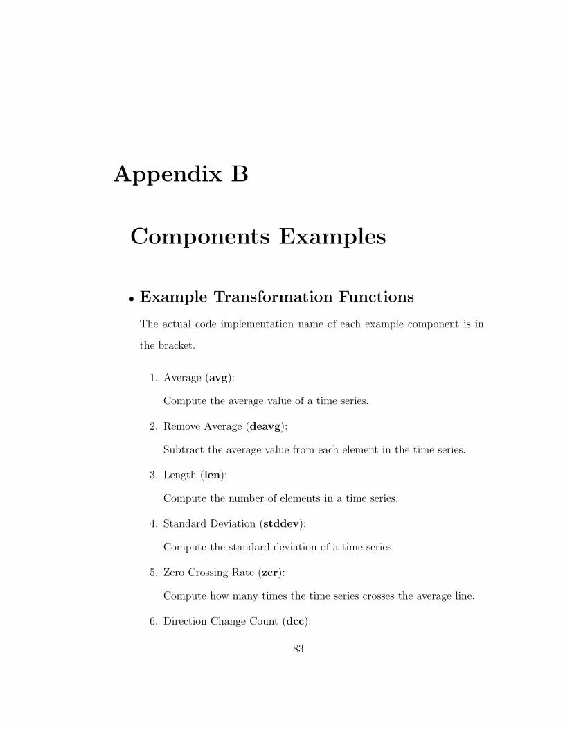
Appendix B
Components Examples
• Example Transformation Functions
The actual code implementation name of each example component is in
the bracket.
1. Average (avg):
Compute the average value of a time series.
2. Remove Average (deavg):
Subtract the average value from each element in the time series.
3. Length (len):
Compute the number of elements in a time series.
4. Standard Deviation (stddev):
Compute the standard deviation of a time series.
5. Zero Crossing Rate (zcr):
Compute how many times the time series crosses the average line.
6. Direction Change Count (dcc):
83

Compute how many times the time series changes direction, either
up or down.
7. Map to Uniform Axis (uni128):
Map the time series to a uniform length (default is 128). It is the same
as the global time scaling function in Section Underlying Technology
2 except that it up-scales the data when the original size is less than
the uniform length and down-scales the data otherwise.
8. Envelope with α%-Warping (env5percent):
Compute the k-Envelope (see Equation 2.3) of the time series where
k is α% ∗ n, where n is the length of the time series. By default,
α = 5.
9. n-PAA: Piecewise Aggregate Approximation (paa8):
Divide the time series into n equal length pieces and average the value
by piece (see Equation 2.7). The result is a time series of length n.
By default, n = 8.
If the input is an envelope time series, the result is still an enve-
lope where the resulting higher (lower) envelope is the n-PAA of the
original higher (lower) envelope.
10. k-DFT: Discrete Fourier Transform (dft8):
Compute the first k real-part coefficients of the Discrete Fourier
Transform of the time series, see reference [28]. By default, k = 8.
11. k-db2-DWT: Discrete Wavelet Transform (db2dwt8):
Compute the first k co-efficient of the db2 Discrete Wavelet
Transform (see reference [28]) of the time series. By default, k = 8.
84

12. k-offset filter (noisefilter):
Low/high-pass filter: delete any element if its value v satisfies |v −
v̄| ≥ k where v̄ is the average value of the time series. It also resets
any value less than 0 as 0.
13. Transform value-duration pair sequence to value sequence (nd2ts):
Given a value-duration pair sequence, X = [(v1, d1), (v2, d2), . . . , (vn, dn)]
where vi is a real number, di is a positive integer for any i, this
transformation function T outputs a real-value time series where vi
is padded di times. E.g. T ([(3, 2), (5, 1), (4, 3)]) = [3, 3, 5, 4, 4, 4].
14. Transform zero-separated value sequence into value-duration pair se-
quence (segts2nd):
Given a zero-separated value sequence X = [V1, 0, V2, 0, . . . , Vn],
where Vi = [Vi(1), Vi(2), . . . , Vi(ki)], ki > 0 for each i,Vi(ji) is a real
number for any 1 ≤ ji ≤ ki, this transformation function T outputs
a value-duration pair sequence Y = [(V̄1, k1), (V̄2, k2), . . . , (V̄n, kn)]
where V̄i is the average of all the values in Vi. E.g. T ([3, 3, 0, 5, 0, 4, 4, 4] =
[(3, 2), (5, 1), (4, 3)].
• Example Comparison Functions
1. Subtraction (subtraction)
C(q, r) = q − r, where q, r are both scalars or both time series of the
same length.
It is reflexive and transitive; its absolute value is symmetric and
satisfies triangle inequality when both input are scalars.
2. Ratio (ratio)
85

C(q, r) = qr− 1
It is reflexive.
3. Normalized Manhattan Distance (manhattan dis)
C(q, r) =P
n
i|qi−ri|
n, where q, r are both time series of the length n
and qi, ri is respectively the i-th element of q, r.
It is reflexive, symmetric, transitive and satisfies triangle inequality.
4. Normalized Euclidean Distance (euclidean)
C(q, r) =P
n
i
√(qi−ri)2
n, where q, r are both time series of the length
n and qi(ri) is the i-th element of q(r).
It is reflexive, symmetric, transitive and satisfies triangle inequality.
5. Normalized Envelope distance (env dis)
C(q, env) =
∑ni envD(qi − envi)
n
where q is a time series of length n, env is an envelope time series of
the length n and qi/envi is the i-th element of q/env.
and
envD(qi, envi) =
0 if bi ≤ qi ≤ ti
qi − ti if qi > ti
bi − qi if qi < bi
where ti, bi are the i-th element of the top/bottom envelope of env.
It is non-reflexive, non-symmetric, non-transitive and does not satisfy
triangle inequality.
6. α%-Local Dynamic Time Warping (ldtw)
86

It computes the k-local dynamic time warping distance between two
time series q, r where k = 1 + n ∗ α% and n is the length of q. See
Equation 2.5. It is reflexive.
87

Appendix C
Feedback on the system
Figure C.1: Google search result top-1 with keywords “query by humming”
The efforts of the team members of the query-by-humming project have
88

Figure C.2: Yahoo search result top-1 with keywords “query by humming”
resulted in our project page being ranked in the top result list by major search
engines if a user searches keywords such as “query by humming”, “whats that
song” and “humming”. See Figure C.1, C.2 and C.3.
Besides the website, our team also participated a tech-show event. “The
demo was a big success. There were more ‘hummers’ than we expected and
there was a lot of enthusiasm and amazement. I prepared mp3-files for the 25
selected titles in the database and so the attendees had the possibility to listen
to the audio-file before humming. Result was much better, when the hummer
listened to the midi-sequence instead of the audio-file before humming. It seems
that for some titles it’s hard to filter a simple melody from a complex title in
mp3 format. But for 70% of the hummers the matching score was very high
89

Figure C.3: MSN search result top-1 with keywords “query by humming”
(ranking 1 or 2) and there were about two persons with bad matching, but not
everyone is really an apt hummer... Sometimes it was very noisy in the demo
room and it seemed to me that this also has had an influence on the matching
score.” — Swiss Broadcasting Company
“ Works like a dream... ” — a user on www.digg.com’s post about us
90

Figure C.4: Screenshot of the web demo
91
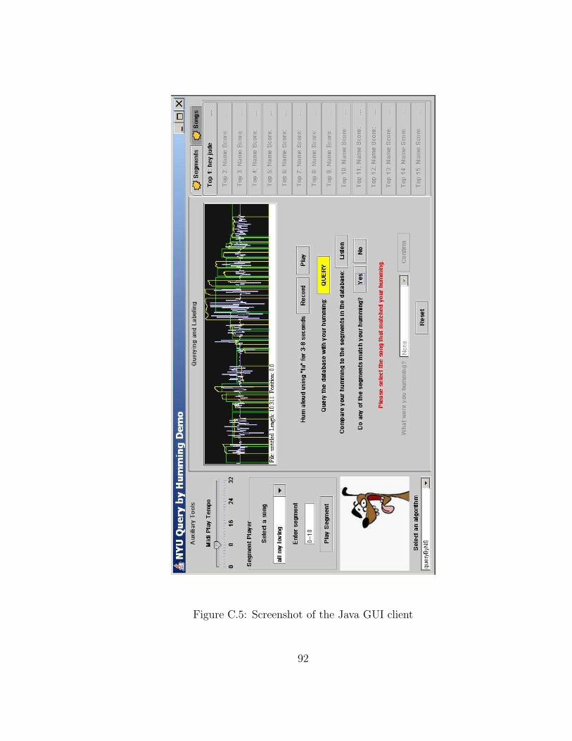
Figure C.5: Screenshot of the Java GUI client
92

Bibliography
[1] http://www.kx.com/.
[2] http://www.nzdl.org/musiclib/.
[3] R. Agrawal, C.Faloutsos, and A.Swami. Efficient similarity search in se-
quence databases. In FODO Conference, volume 730, 1993.
[4] W. A. Arentz, M. L. Hetland, and B. Olstad. Methods for retrieving musical
information based on rhythm and pitch correlation. In CSGSC, 2003.
[5] D. Berndt and J. Clifford. Using dynamic time warping to find patterns in
time series. In Advances in Knowledge Discovery and Data Mining, pages
229–248. AAAI/MIT, 1994.
[6] P. Cano, E. Batlle, T. Kalker, and J. Haitsma. A review of algorithms for
audio fingerprinting. In MMSP, 2002.
[7] K. P. Chan and A. W. C. Fu. Efficient time series matching by wavelets. In
In proceedings of the 15th International Conference on Data Engineering,
pages 126–133, Sydney, Australia, 1999.
93

[8] A. W. chee Fu, E. Keogh, L. Y. H. Lau, and C. A. Ratanamahatana.
Scaling and time warping in time series querying. In Proceedings of the
31st VLDB Conference, Trondheim, Norway, 2005.
[9] S. Chu, E. Keogh, D. Hart, and M. Pazzani. Iterative deepening dynamic
time warping for time series. In Unkown, 2002.
[10] C. Faloutsos, M. Ranganathan, and Y. Manolopoulos. Fast subsequence
matching in time-series databases. In Proceedings 1994 ACM SIGMOD
Conference, Mineapolis, MN, USA, 1994.
[11] Y. Freund and R. Schapire. Experiments with a new boosting algorithm.
In In Proceedings of the Thirteenth International Conference on Machine
Learning, pages 148–156, 1996.
[12] D. Gunopulos and G. Das. Time series similarity measures. In SIGKDD
Tutorial, 2002.
[13] E. Keogh. A tutorial on indexing and mining time series data. In ICDM
’01.The 2001 IEEE International Conference on Data Mining, San Jose,
November 29 2001.
[14] E. Keogh. Exact indexing of dynamic time warping. In VLDB, pages
406–417, Hong Kong, China, 2002.
[15] E. Keogh, K. Chakrabarti, S. Mehrotra, and M. Pazzani. Locally adaptive
dimensionality reduction for indexing large time series databases. In ACM
SIGMOD International Conference on Management of Data, 2001.
[16] E. Keogh, K. Chakrabarti, M. Pazzani, and S. Mehrotra. Dimensionality
reduction for fast similarity search in large time. In KAIS, 2000.
94

[17] F. Korn, H. V. Jagadish, and C. Faloutsos. Efficiently supporting ad hoc
queries in large datasets of time sequences. In SIGMOD 1997, Proceedings
ACM SIGMOD International Conference on Management of Data, pages
289–300, Tucson, Arizona USA, May 13-15 1997.
[18] N. Kosugi. A study on content-based music retrieval with humming. Ph.D.
Thesis, 2005.
[19] N. Kosugi, Y. Nishihara, T. Sakata, M. Yamamuro, and K. Kushima. A
pratical query-by-humming system for a large music database. In ACM
Multimedia 2000, pages 333–342, 2000.
[20] D. Mazzoni and R. B. Dannenberg. Melody matching directly from au-
dio. In In 2nd Annual International Symposium on Music Information
Retrieval, Bloomington, Indiana, USA, 2001.
[21] R. J. McNab, L. A. Smith, D. Bainbridge, and I. H.
Witten. The new zealand digital library melody index.
http://www.dlib.org/dlib/may97/meldex/05witten.html.
[22] I. Popivanov and R. Miller. Similarity search over time series data us-
ing wavelets. In 18th International Conference on Data Engineering
(ICDE’02), 2002.
[23] D. Rafiei and A. Mendelzon. Similarity-based queries for time series data.
In Proceeding of ACM SIGMOD International Conference on Management
of Data, pages 13–25, 1997.
[24] C. A. Ratanamahatana and E. Keogh. Making time-series classification
more accurate using learned constraints.
95

[25] C. Rudin, I. Daubechies, and R. E. Schapire. On the dynamics of boosting.
In To appear with Revisions in NIPS Proceedings, 2003, 2003.
[26] R. E. Schapire and Y. Singer. Improved boosting using confidence-rated
predictions. Machine Learning, 37(3):297–336, 1999.
[27] X. Shao, C. Xu, and M. S. Kankanhalli. Qbh2 - a query by humming
retrieval system based on polyphonic karaoke music database. Submitted
to IEEE Transactions on Multimedia, 2006.
[28] D. Shasha and Y. Zhu. High Performance Discovery in Time Series.
Springer Verlag, 2004.
[29] S. Theodoridis and K. Koutroumbas. Pattern recognition. San Diego :
Academic Press, 1999.
[30] R. T. Trevor Hastie and J. Friedman. The elements of sattistical Learning:
Data mining, inference and prediction. Springer, 2003.
[31] A. Uitdenboderd and J. Zobel. Melodic matching techniques for large music
databases. ACM Multimedia 99, 1999.
[32] Y.-L. Wu, D. Agrawal, and A. E. Abbadi. A comparison of dft and dwt
based similarity search in time-series databases. Technical Report TRCS00-
08, University of California, Santa Barbara, 2000.
[33] B.-K. Yi and C. Faloutsos. Fast time sequence indexing for arbitrary lp
norms. In VLDB 2000, Proceedings of 26th International Conference on
Very Large Data Bases, pages 385–394, Cairo, Egypt, Sep. 10-14 2000.
96

[34] X. Zhao. High performance correlation techniques for time series. Thesis
Proposal, New York University, 2004.
[35] Y. Zhu, M. S. Kankanhalli, and C. Xu. Pitch tracking and melody slope
matching for song retrieval. In Advances in Multimedia Information Pro-
cessing PCM 2001, Second IEEE Pacific Rim Conference on Multimedia,
pages 24–26, Beijing China, October 2001.
[36] Y. Zhu and D. Shasha. Statstream: Statistical monitoring of thousands of
data streams in real time. In VLDB 2002, Proceeding of 28th International
Conference on Very Large DataBases, pages 358–369, Hong Kong, China,
August 20-23 2002.
[37] Y. Zhu, D. Shasha, and X. Zhao. Query by humming: in action with its
technology revealed. Proceedings of the 2003 ACM SIGMOD international
conference on on Management of data, June 2003.
97
Top Related