


Languages
Pages
Legal


c© Copyright by
QI YE
May 2012
ii

ACKNOWLEDGMENT
I would like to express my deep and sincere gratitude to my advisor, Prof. Gregory
E. Fasshauer of Illinois Institute of Technology (IIT). He patiently taught me everything I
know about meshfree approximation methods in general. In particular, he directed me to
think of the relationship between Green functions and reproducing kernels. I would like to
gratefully acknowledge him for spending his time and energy for my papers and researches.
I would like to thank my parents, Ruizhi Ye and Yinan Shen. They encouraged me
to pursue my Ph.D. degree in the United States.
I would also like to acknowledge the following people for their assistance: Prof.
Fred Hickernell of IIT for helpful comments and discussions in the meshfree seminar, Prof.
Igor Cialenco of IIT for the help with stochastic partial differential equations, Prof. Geof-
frey Williamson of IIT for sitting on my comprehensive exam committee, Prof. Gady Agam
of IIT for sitting on my dissertation exam committee, Prof. Kendall Atkinson of Univ. of
Iowa for providing valuable suggestions on eigenvalues and eigenfunctions of Green ker-
nels, Prof. Jinqiao Duan of IIT who taught me stochastic analysis, Prof. Xiaofan Li of
IIT for guiding my registration of graduate courses, and Mrs. Gladys Collins of IIT for
administrative assistance with my student events at IIT.
Finally, I would like to thank all committee members of the IIT SIAM chapter for
their help with organizing the SIAM Student Chapter Conference 2011.
iii

TABLE OF CONTENTS
Page
ACKNOWLEDGEMENT . . . . . . . . . . . . . . . . . . . . . . . . . . iii
LIST OF FIGURES . . . . . . . . . . . . . . . . . . . . . . . . . . . . . vi
LIST OF SYMBOLS . . . . . . . . . . . . . . . . . . . . . . . . . . . . vii
ABSTRACT . . . . . . . . . . . . . . . . . . . . . . . . . . . . . . . . xii
CHAPTER1. INTRODUCTION . . . . . . . . . . . . . . . . . . . . . . . . 1
1.1. Reproducing Kernels and Green Functions . . . . . . . . . . 41.2. Application of Reproducing Kernels . . . . . . . . . . . . . 6
2. KERNEL-BASED METHODS . . . . . . . . . . . . . . . . . . 8
2.1. Reproducing Kernel Hilbert Spaces and Positive Definite Kernels 82.2. Conditionally Positive Definite Functions on the Whole Space . 92.3. Positive Definite Kernels on Bounded Domains . . . . . . . . 122.4. Error Estimates in Terms of Fill Distance . . . . . . . . . . . 132.5. Optimal Recovery . . . . . . . . . . . . . . . . . . . . . . 14
3. DISTRIBUTION AND TRANSFORM ANALYSIS . . . . . . . . 15
3.1. Test Functions and Tempered Distributions . . . . . . . . . . 163.2. Differential Operators and Distributional Operators . . . . . . 183.3. Fourier Transforms and Distributional Fourier Transforms . . . 223.4. Boundary Operators . . . . . . . . . . . . . . . . . . . . . 24
4. CONSTRUCTING CONDITIONALLY POSITIVE DEFINITE FUNC-TIONS VIA GREEN FUNCTIONS . . . . . . . . . . . . . . . . 27
4.1. Green Functions on the Whole Space . . . . . . . . . . . . . 274.2. Constructing Generalized Sobolev Spaces with Distributional Op-
erators on the Whole Space . . . . . . . . . . . . . . . . . 294.3. Examples . . . . . . . . . . . . . . . . . . . . . . . . . . 37
5. CONSTRUCTING POSITIVE DEFINITE KERNELS VIA GREENKERNELS . . . . . . . . . . . . . . . . . . . . . . . . . . . 44
5.1. Preparations . . . . . . . . . . . . . . . . . . . . . . . . 445.2. Green Kernels on Bounded Domains . . . . . . . . . . . . . 525.3. Constructing Generalized Sobolev Spaces with Differential Op-
erators and Boundary Operators on Bounded Domains . . . . . 54
iv

5.4. Examples . . . . . . . . . . . . . . . . . . . . . . . . . . 70
6. REPRODUCING KERNEL BANACH SPACES . . . . . . . . . . 75
6.1. Constructing Reproducing Kernel Banach Spaces via PositiveDefinite Functions . . . . . . . . . . . . . . . . . . . . . 76
6.2. Optimal Recovery in Reproducing Kernel Banach Spaces . . . 816.3. Examples of Matern Functions . . . . . . . . . . . . . . . . 82
7. APPROXIMATION OF STOCHASTIC PARTIAL DIFFERENTIALEQUATIONS VIA KERNEL-BASED COLLOCATION METHODS 84
7.1. Classical Data Fitting Problems . . . . . . . . . . . . . . . 857.2. Constructing Gaussian Fields by Reproducing Kernels . . . . . 897.3. Constructing Gaussian Fields by Reproducing Kernels with Dif-
ferential and Boundary Operators . . . . . . . . . . . . . . 917.4. Approximation of Elliptic Partial Differential Equations . . . . 947.5. Approximation of Elliptic Stochastic Partial Differential Equations 1007.6. Approximation of Parabolic Stochastic Partial Differential Equa-
tions . . . . . . . . . . . . . . . . . . . . . . . . . . . . 108
8. FUTURE WORK . . . . . . . . . . . . . . . . . . . . . . . . 118
8.1. Pseudo-differential Operators . . . . . . . . . . . . . . . . 1188.2. Singular Green Kernels . . . . . . . . . . . . . . . . . . . 1188.3. Optimal Shape Parameters . . . . . . . . . . . . . . . . . . 1198.4. Kernel-based Collocation Methods for SPDEs . . . . . . . . . 120
APPENDIX . . . . . . . . . . . . . . . . . . . . . . . . . . . . . . . . . 121
A. WHITE NOISE AND STOCHASTIC PARTIAL DIFFERENTIAL EQUA-TIONS . . . . . . . . . . . . . . . . . . . . . . . . . . . . . 121
BIBLIOGRAPHY . . . . . . . . . . . . . . . . . . . . . . . . . . . . . . 123
v

LIST OF FIGURES
Figure Page
1.1 Qi Ye’s mathematical ancestry tree traced back to Gauß . . . . . . . 2
1.2 Numerical Experiments for Gaussian Kernels. . . . . . . . . . . . . 3
7.1 Numerical Experiments for PDE (7.4). . . . . . . . . . . . . . . . 100
7.2 Convergence Rates for PDE (7.4). . . . . . . . . . . . . . . . . . 101
7.3 Numerical Experiments for SPDE (7.6). . . . . . . . . . . . . . . . 107
7.4 Convergence Rates for SPDE (7.6). . . . . . . . . . . . . . . . . . 107
7.5 Numerical Experiments of Distributions for SPDE (7.11). . . . . . . 115
7.6 Numerical Experiments of Mean and Variance for SPDE (7.11). . . . . 116
7.7 Convergence Rates for SPDE (7.11). . . . . . . . . . . . . . . . . 117
vi

LIST OF SYMBOLS
Symbol Definition
Nd space of d-dimensional positive integers
Nd0 space of d-dimensional nonnegative integers
R+0 nonnegative real numbers
R+ positive real numbers
Rd d-dimensional real Euclidean space
D connected subset (domain) of Rd
D closure ofD
∂D boundary ofD
XD collocation points in the domainD
X∂D collocation points on the boundary ∂D
δx Dirac delta function (Dirac delta distribution) at the point x,page 18
hX,D fill distance of data points X for a domainD, page 13
δ jk Kronecker delta function, page 52
G Green function or Green kernel, page 27, 52
Φ conditionally positive definite function, page 9
K reproducing kernel, page 8
∗
K integral-type kernel of the reproducing kernel K, page 89
ˆ Fourier transform, page 22
ˇ inverse Fourier transform, page 22
Φm generalized Fourier transform of order m of Φ, page 23
vii
α α := (α1, · · · , αd)T∈ Nd
0
|α|∑d
k=1 αk
α!∏d
k=1 αk
Dα derivative∏d
k=1∂αk
∂xαkk
of order α, page 13
Dβ|∂D trace mapping of the βth derivative Dβ defined on ∂D, page 25
P differential operator or distributional operator, page 19
P∗ distributional adjoint operator of P, page 19
O(P) order of differential operator P, page 20
P vector differential operator or vector distributional operator
B boundary operator, page 26
O(B) order of boundary operator B, page 26
B vector boundary operator
I identity operator
∆ Laplace differential operator
IK,D integral operator defined by(IK,D f
)(x) :=
∫D
K(x, y) f (y)dx,page 12
f = O(g) | f | ≤ C |g| for a positive constant C
f = Θ(g) C1 |g| ≤ | f | ≤ C2 |g| for two positive constants C1, C2
B1 B2 B1 and B2 are isomorphic, page 15
B1 ≡ B2 B1 and B2 are isometrically isomorphic, page 15
Re (F ) restriction of the function space F to the real field
B (B) Borel σ-field of the Banach space B
S test functions defined on Rd, page 16
viii

S2m special subspace of S consisting of functions with at most like apolynomial of degree 2m at the origin, page 17
D test functions defined onD, page 17
T S or D , page 18
F ′ dual space of topological vector space (TVS) F
SI collection of slowly increasing functions, page 17
πm−1(Rd) space of polynomials degree less than m
C∞(D) ∩∞m=0Cm(D)
C∞0 (D) all functions in C∞(D) that have compact support onD
C∞b (D) all functions in C∞(D) which, together with all their partialderivatives, are bounded onD
Hm(D) L2-based Sobolev space of order m defined onD, page 21
Hm0 (D) completion of Cm
0 (D) with respect to theHm(D)-norm, page 22
Wmp (D) Lp-based Sobolev space of order m defined onD, page 22
HP(Rd) generalized Sobolev space induced by a vector distributional op-erator P defined on Rd, page 29
H0P(D) generalized Sobolev space with homogeneous boundary condi-
tions defined onD, page 54
HAB (D) a special subspace of Null(L) to construct nonhomogeneous
boundary conditions on ∂D (see Definition 5.8), page 59
HAPB(D) real generalized Sobolev space with nonhomogeneous boundary
conditions defined onD, page 62
HK(D) reproducing kernel Hilbert space with a reproducing kernel K de-fined onD, page 8
N0Φ
(Rd) native space associated with a positive definite function Φ,page 11
ix

NmΦ
(Rd) native space associated with a conditionally positive definite func-tion Φ of order m, page 11
BpΦ
(Rd) reproducing kernel Banach space associated with the positive def-inite function Φ and p ≥ 2, page 77
HD2(R2) Duchon semi-norm space defined on R2, page 37
H∆(R2) Laplacian semi-norm space on R2, page 38
BLm(Rd) Beppo-Levi space of order m on Rd, page 39
Lp(Rd; µ) Lp-based space defined on Rd with the positive measure µ,page 77
Null(L) f ∈ Hm(D) : L f = 0 for a differential operator L of order 2m,page 50
Null(P) f ∈ Hm(D) : P f = 0 for a vector differential operator P of orderm, page 45
PmD
a special subset of vector differential operators defined onHm(D)(see Definition 5.1), page 45
BmD
a special subset of vector boundary operators defined on Hm(D)(see Definition 5.2), page 49
( f , g)D∫D
f (x)g(x)dx, page 45
( f , g)∂D∫∂D
f (x)g(x)dS (x), page 48
( f , g)m,D∑|α|≤m
∫D
Dα f (x)Dαg(x)dx, page 21
( f , g)P,D∑∞
j=1
∫D
P j f (x)P jg(x)dx, page 29, 45
( f , g)B,∂D∑n
j=1
∫∂D
B j f (x)B jg(x)dS (x), page 48
〈γ,T 〉F T (γ) for all γ ∈ F and all T ∈ F ′ where F is a TVS.
(Ω,F ,P) Ω: sample space, F : filtration, P: probability measure
E (U) mean of the random variable U
Var (U) variance of the random variable U
x

Cov (U1,U2) covariance of the random variables U1 and U2
S x stochastic Gaussian process, page 85
Wt Brownian motion or Wiener noise, page 122
xi

ABSTRACT
In this thesis, we use Green functions (kernels) to set up reproducing kernels such
that their related reproducing kernel Hilbert spaces (native spaces) are isometrically em-
bedded into or even are isometrically equivalent to generalized Sobolev spaces. These
generalized Sobolev spaces are set up with the help of a vector distributional operator P
consisting of finitely or countably many elements, and possibly a vector boundary operator
B. The above Green functions can be computed by the distributional operator L := P∗T P
with possible boundary conditions given by B. In order to support this claim we ensure that
the distributional adjoint operator P∗ of P is well-defined in the distributional sense. The
types of distributional operators we consider include not only differential operators but also
more general distributional operators such as pseudo-differential operators. The general-
ized Sobolev spaces can cover even classical Sobolev spaces and Beppo-Levi spaces. The
well-known examples covered by our theories include thin-plate splines, Matern functions,
Gaussian kernels, min kernels and others. As an application for high-dimensional approxi-
mations, we can use the Green functions to construct a multivariate minimum-norm inter-
polant s f ,X to interpolate the data values sampled from an unknown generalized Sobolev
function f at data sites X ⊂ Rd. Moreover, we also use Green functions to set up repro-
ducing kernel Banach spaces, which can be equivalent to classical Sobolev spaces. This is
a new tool for support vector machines. Finally, we show that stochastic Gaussian fields
can be well-defined on the generalized Sobolev spaces. According to these Gaussian-field
constructions, we find that kernel-based collocation methods can be used to approximate
the numerical solutions of high-dimensional stochastic partial differential equations.
xii

1
CHAPTER 1
INTRODUCTION
The theory and practice of kernel-based approximation methods is a fast growing
research area. It has been used for high-dimensional approximation and statistical learn-
ing. Moreover, their applications come from such different fields as applied mathematics,
computer science, geology, biology, engineering, and even finance.
History:
The well-known positive definite kernel, Gaussian kernel with
shape parameter σ > 0 (see Example 4.5), i.e.,
K(x, y) := e−σ2 |x−y|2 , x, y ∈ R,
is closely associated with Carl Friedrich Gauß. Gauß mentioned
the kernel function that now so often carries his name in 1809 in
his second book – Theory of the motion of the heavenly bodies
moving about the sun in conic sections [23].
Carl Friedrich Gauß
1777-1855
(painted by Christian Albrecht Jensen)
In the beginning of the analysis of the kernel-based methods, Maximilian Mathias
was chiefly concerned with positive definite functions in 1923 (see [38]), and James Mer-
cer had considered the more general concept of positive definite kernels in 1909 (see [40]).
Later Salomon Bochner [6] and Iso Schoenberg [51] made fundamental contributions for
characterizations of positive definite functions in terms of Fourier transforms. Aleksandr
Khinchin [32] further used Bochner’s theoretical results to set up stationary stochastic pro-
cesses in probability theory. Micchelli [41, 42] started the work for conditionally positive
definite functions. Schaback [47] and Wendland [59] found the compactly supported radial
basis functions. Stewart’s survey [56] and Fasshauer’s survey [19] described much more

2
detail of the history and the background for positive definite kernels. There are many text
books for the applications of the kernel-based methods, e.g., meshfree approximation meth-
ods and radial basis functions [8, 18, 28, 60] and support vector machines and statistical
learning [3, 24, 55].
Carl Friedrich Gauß
Christian Gerling
Julius Plücker
Friedrich Bessel
Felix Klein
Carl Louis Lindemann
David Hilbert
Erhard Schmidt
Maximilian Mathias
Salomon Bochner
Richard Courant
Samuel Karlin
Charles Micchelli
Franz Rellich
Erhard Heinz
Helmut Werner
Robert Schaback
Armin Iske
Holger Wendland
Larry Schumaker
Greg Fasshauer
Qi Ye
Page 1 of 1
2012-3-4file://D:\My Paper\PhD Thesis\Advisor_Tree.htm
Figure 1.1. Qi Ye’s mathematical ancestry tree traced back to Gauß

3
We display a mathematical ancestry tree of Qi Ye to show how the work presented
in this thesis is connected by a smooth and direct path to Carl Friedrich Gaußbased on
the data available at [1] in Figure 1.1. Many of the names listed in the ancestry chart
made significant contributions to the foundations of kernel-based approximation methods,
e.g., Gauß, Bessel, Hilbert, Schmidt, Mathias, Bochner, Karlin, Micchelli, Schaback, Iske,
Wendland and Fasshauer. In this thesis, we want to develop a clear and detailed framework
of the relations between Green functions (kernels) and reproducing kernels in order to build
up a new analysis tool for their related native spaces (reproducing kernel Hilbert or Banach
space) and apply them to practical problems such as support vector machines and stochastic
partial differential equations.
00.5
1
0
0.5
1
−0.5
0
0.5
1
1.5
Interpolation Data
00.5
1
0
0.5
1
−0.5
0
0.5
1
1.5
Franke Function
00.5
1
0
0.5
1
−0.5
0
0.5
1
1.5
Approximate Solution
0
0.5
1
0
0.5
1
0
0.05
0.1
Point−wise Error
Error−0.02 0 0.02 0.04 0.06 0.08
X-Halton points with N = 81, f -Franke’s function, K-Gaussian kernel with σ = 3.6.
Figure 1.2. Numerical Experiments for Gaussian Kernels.
Generally speaking, the fundamental underlying practical problem common to many
of the kernel-based applications can be represented in the following way. Given a set of

4
data sites X := x1, . . . , xN ⊂ D ⊆ Rd and associated values Y := y1, . . . , yN ⊂ R sampled
from an unknown function f , we will use a reproducing kernel K : D×D → R to set up an
interpolant s f ,X to approximate the function f at the data sites (see Figure 1.2). The domain
D can be quite arbitrary except that it should contain at least one point. When f belongs
to the associated function space (native space) of the kernel K, we are able to obtain error
bounds and optimality properties of this interpolation method (see e.g., Chapter 2). The
native space can be a reproducing kernel Hilbert space.
Some of the interesting open problems in need to be answered for the kernel meth-
ods are: what kind of functions belong to the related native space of a given kernel function,
and which kernel function is the best for us to utilize for a particular application? In partic-
ular, a better understanding of the native space in relation to traditional smoothness spaces
(such as Sobolev spaces) is highly desirable (see e.g., [8, 18, 48, 60]). The latter question
is partially addressed by the use of techniques such as cross-validation and maximum like-
lihood estimation to obtain optimally scaled kernels for any particular application (see e.g.,
[5, 54, 58]). However, at the function space level, the question of scale is still in need of a
satisfactory answer.
1.1 Reproducing Kernels and Green Functions
We deal with these questions in a different way than most people have done before.
In my research and published papers [20, 21, 61], we show that the reproducing kernel and
its native space can be computed via a Green function (kernel) and a generalized Sobolev
space, respectively, induced by a vector distributional operator P := (P1, · · · , Pn, · · · )T
(consisting of finitely or countably many elements) and possibly a vector boundary operator
B := (B1, · · · , Bn)T defined as in Chapters 4 and 5. Moreover, the inner product of this
native space has an explicit form induced by the related operators. This idea comes from the
theoretical work of Duchon on thin-plate splines [14], who may have been the first person
making the connections of Green functions and radial basis functions for interpolation of

5
scattered data in 1976. Since then, there have been only a few papers concerned with the
relationships for Green functions and reproducing kernels. In Chapters 4 and 5, we show
the relations between Green functions and conditional positive definite functions and find
the connections of Green kernels and positive definite kernels, respectively.
Why do we use different vector distributional operators to set up the generalized
Sobolev space? An important feature driving this definition is the fact that this will give us
different norms in which to measure the target function f adding a notion of scale on top
of the usual smoothness properties. As we discuss in Example 1.1, a shape parameter will
control the norm by affecting the weight of the various derivatives involved. This may guide
us in finding the kernel function with “optimal” shape parameter to set up a kernel-based
approximation for a given set of data values — an important problem in practice for which
no analytical solution exists. Example 4.4 tells us that we can balance the role of different
derivatives by selecting appropriate shape parameters when reconstructing the classical
Sobolev spaces by starting with appropriately chosen inner products for our generalized
Sobolev spaces.
Example 1.1. We consider two positive definite functions for differently scaled versions of
the classical L2-based Sobolev spaceH2(R): the function
G(x) := e−√
32 |x| sin
(12|x| +
π
6
), x ∈ R,
and the Matern function
Gσ(x) :=1
8σ3(1 + σ |x|) e−σ|x|, x ∈ R,
with shape parameter σ > 0. Let P :=(
d2
dx2 ,ddx , I
)Tand Pσ :=
(d2
dx2 ,√
2σ ddx , σ
2I)T
. It is not
difficult to show that G and Gσ are full-space Green functions of the differential operators
L := P∗T P = I − d2
dx2 + d4
dx4 and Lσ := P∗Tσ Pσ =(σ2I − d2
dx2
)2, respectively. As a result the
inner products for the generalized Sobolev spaces are
( f , g)HP(R) :=∫R
(f ′′(x)g′′(x) + f ′(x)g′(x) + f (x)g(x)
)dx, f , g ∈ HP(R) ≡ H2(R),

6
and
( f , g)HPσ (R) :=∫R
(f ′′(x)g′′(x) + 2σ2 f ′(x)g′(x) + σ4 f (x)g(x)
)dx, f , g ∈ HPσ(R) H2(R).
According to Proposition 4.7, we can show that they are isometrically equivalent to the re-
producing kernel Hilbert spacesHK(R) andHKσ(R) with the reproducing kernels K(x, y) :=
G(x − y) and Kσ(x, y) := Gσ(x − y), respectively.
This example shows that it may make sense to redefine the classical Sobolev space
employing different inner products in terms of shape parameters even though HP(R) ≡
HK(R) andHPσ(R) ≡ HKσ(R) are composed of functions with the same smoothness prop-
erties and are not distinguished under standard Hilbert space theory (i.e., considered iso-
morphic). These different inner products provide us with a clearer understanding of the
important role of the shape parameter. This formulation allows us to think of σ−1 as the
natural length scale dependent on the weight of various derivatives. The choice of smooth-
ness and scale now tell us which kernel to use for a particular application. This choice
may be performed by the user based on some a priori knowledge of the problem and based
directly on the data.
1.2 Application of Reproducing Kernels
Based on our theoretical results of reproducing kernels, we can also use the kernel-
based method to conduct applications such as on stochastic partial differential equations,
statistical learning and random dynamical systems.
In Chapter 6, we also use the positive definite functions to set up the reproducing
kernel Banach spaces. This provides a new tool for the support vector machines similar as
done in [3, 24, 55]. Moreover, if we use Matern functions to construct reproducing ker-
nels, then their related reproducing kernel Banach spaces can be equivalent to the classical
Sobolev spaces.
7
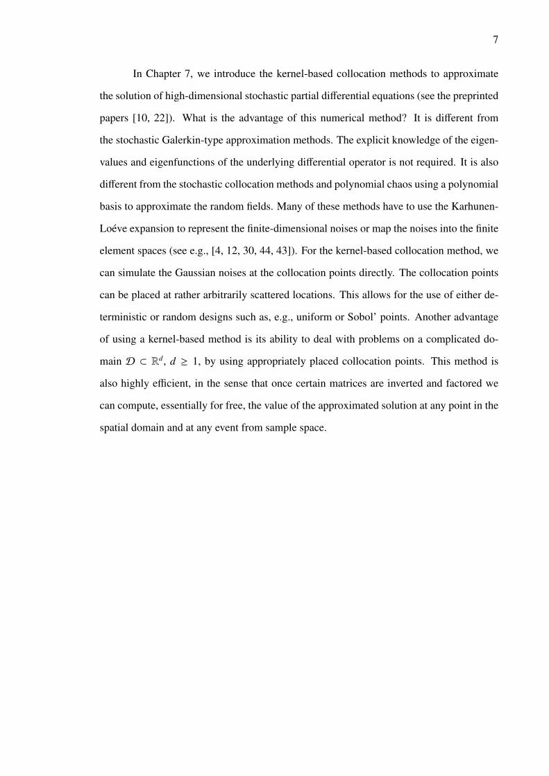
In Chapter 7, we introduce the kernel-based collocation methods to approximate
the solution of high-dimensional stochastic partial differential equations (see the preprinted
papers [10, 22]). What is the advantage of this numerical method? It is different from
the stochastic Galerkin-type approximation methods. The explicit knowledge of the eigen-
values and eigenfunctions of the underlying differential operator is not required. It is also
different from the stochastic collocation methods and polynomial chaos using a polynomial
basis to approximate the random fields. Many of these methods have to use the Karhunen-
Loeve expansion to represent the finite-dimensional noises or map the noises into the finite
element spaces (see e.g., [4, 12, 30, 44, 43]). For the kernel-based collocation method, we
can simulate the Gaussian noises at the collocation points directly. The collocation points
can be placed at rather arbitrarily scattered locations. This allows for the use of either de-
terministic or random designs such as, e.g., uniform or Sobol’ points. Another advantage
of using a kernel-based method is its ability to deal with problems on a complicated do-
main D ⊂ Rd, d ≥ 1, by using appropriately placed collocation points. This method is
also highly efficient, in the sense that once certain matrices are inverted and factored we
can compute, essentially for free, the value of the approximated solution at any point in the
spatial domain and at any event from sample space.

8
CHAPTER 2
KERNEL-BASED METHODS
Most of the material presented in this chapter can be found in the excellent mono-
graphs [18, 60]. For the reader’s convenience we repeat what is essential to our discussion
later on. Their theoretical results for real-valued kernels can be extended to the complex
field in a very similar way. The only difference is that in the complex case special care has
to be taken with the complex conjugate sign.
2.1 Reproducing Kernel Hilbert Spaces and Positive Definite Kernels
We are interested in linear vector spaces consisting of functions f : D → C defined
on a domainD of Rd. The domainD can be quite arbitrary except that it should contain at
least one point. For convenience, we fix each domainD to be a connected set of Rd.
Definition 2.1 ([60, Definition 10.1]). Let H be a Hilbert space consisting of functions
f : D → C. H is called a reproducing kernel Hilbert space and a kernel K : D ×D → C
is called a reproducing kernel forH if
(i) K(·, y) ∈ H , for all y ∈ Rd,
(ii) f (y) = ( f ,K(·, y))H , for all f ∈ H and all y ∈ Rd,
where (·, ·)H is used to denote the inner product ofH .
According to [60, Theorem 10.2], H is a reproducing kernel Hilbert space if and
only if the point evaluation functionals δy belong to the dual space H ′ ≡ H of H for all
y ∈ D. [60, Theorem 10.4] shows that the reproducing kernel is positive semi-definite.
Definition 2.2 ([60, Definition 6.24]). A continuous symmetric K : D ×D → C is called
positive definite on D ⊆ Rd if, for all N ∈ N, all sets of pairwise distinct centers X =
x1, . . . , xN ⊂ D, the quadratic formN∑
j=1
N∑k=1
c jckK(x j, xk) = c∗AK,X c > 0, for all c := (c1, · · · , cN)T∈ CN\0,
9
where the interpolation matrix AK,X :=(K(x j, xk)
)N,N
j,k=1∈ CN×N and c∗ := cT .
This shows that K is positive definite if and only if AK,X is positive definite for any
data sites X. Here, we call K symmetric if K(x, y) = K(y, x).
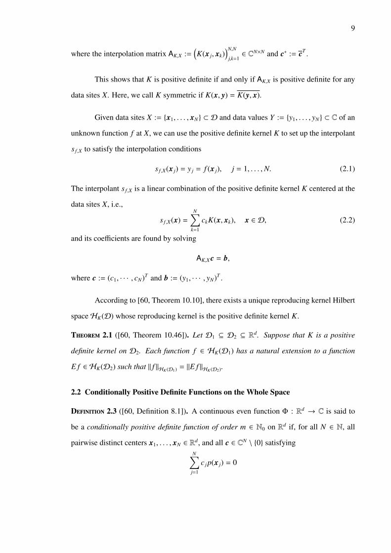
Given data sites X := x1, . . . , xN ⊂ D and data values Y := y1, . . . , yN ⊂ C of an
unknown function f at X, we can use the positive definite kernel K to set up the interpolant
s f ,X to satisfy the interpolation conditions
s f ,X(x j) = y j = f (x j), j = 1, . . . ,N. (2.1)
The interpolant s f ,X is a linear combination of the positive definite kernel K centered at the
data sites X, i.e.,
s f ,X(x) =
N∑k=1
ckK(x, xk), x ∈ D, (2.2)
and its coefficients are found by solving
AK,X c = b,
where c := (c1, · · · , cN)T and b := (y1, · · · , yN)T .
According to [60, Theorem 10.10], there exists a unique reproducing kernel Hilbert
spaceHK(D) whose reproducing kernel is the positive definite kernel K.
Theorem 2.1 ([60, Theorem 10.46]). Let D1 ⊆ D2 ⊆ Rd. Suppose that K is a positive
definite kernel on D2. Each function f ∈ HK(D1) has a natural extension to a function
E f ∈ HK(D2) such that ‖ f ‖HK (D1) = ‖E f ‖HK (D2).
2.2 Conditionally Positive Definite Functions on the Whole Space
Definition 2.3 ([60, Definition 8.1]). A continuous even function Φ : Rd → C is said to
be a conditionally positive definite function of order m ∈ N0 on Rd if, for all N ∈ N, all
pairwise distinct centers x1, . . . , xN ∈ Rd, and all c ∈ CN \ 0 satisfying
N∑j=1
c j p(x j) = 0

10
for all polynomials of degree less than m, p ∈ πm−1(Rd), the quadratic formN∑
j=1
N∑k=1
c jckΦ(x j − xk) = c∗AΦ,X c > 0,
where the interpolation matrix AΦ,X :=(Φ(x j − xk)
)N,N
j,k=1∈ CN×N . In the case m = 0 with
π−1(Rd) := 0 the function Φ is called positive definite on Rd.
We can combine the conditionally positive definite function Φ and a basisp1, . . . , pQ
of the polynomial space πm−1(Rd) to construct an interpolant s f ,X to satisfy the additional
interpolation conditions (2.1), where Q denotes the dimension of πm−1(Rd). The interpolant
is written as
s f ,X(x) =
N∑k=1
ckΦ(x − xk) +
Q∑l=1
βlql(x), x ∈ Rd,
and its coefficients are uniquely obtained by solving a linear equations systemAΦ,X P
P∗ 0
c
β
=
b
0
,where β :=
(β1, · · · , βQ
)T and P :=(pk(x j)
)N,Q
j,k=1∈ CN×Q.
We can use Fourier transform techniques to check whether a function is a condi-
tionally positive definite function.
Theorem 2.2 ([60, Theorem 8.12]). Suppose an even function Φ ∈ C(Rd) ∩ SI possesses
the generalized Fourier transform Φm of order m which is continuous on Rd \ 0. Then Φ is
conditionally positive definite of order m if and only if Φm is nonnegative and nonvanishing.
Here the slowly increasing functions SI and the generalized Fourier transform are
defined in Section 3.1 and 3.3, respectively. We say a complex function Φ is even if Φ(x) =
Φ(−x).
The conditionally positive definite function Φ can be used to create a reproducing
kernel and its reproducing kernel Hilbert space. We firstly set up a native space NmΦ
(Rd)

11
as in [60, Definition 10.16]. NmΦ
(Rd) is a complete semi-inner product space and its null
space is given by πm−1(Rd), i.e., f ∈ NmΦ
(Rd) and | f |NmΦ
(Rd) = 0 if and only if f ∈ πm−1(Rd) ⊆
NmΦ
(Rd). The native space can be characterized by using generalized Fourier transforms.
Theorem 2.3 ([60, Theorem 10.21]). Suppose that Φ is a conditionally positive definite
function of order m ∈ N0. Further suppose that Φ has the generalized Fourier transform
Φm of order m which is continuous on Rd \ 0. Then its native space is characterized by
NmΦ (Rd) =
f ∈ C(Rd) ∩ SI : f has a generalized Fourier transform f
of order m/2 such that f/Φ1/2
m ∈ L2(Rd),
and its semi-inner product satisfies
( f , g)NmΦ
(Rd) = (2π)−d/2∫Rd
f (x)g(x)Φm(x)
dx.
According to [60, Theorem 10.20],NmΦ
(Rd) will become a reproducing kernel Hilbert
spaceHK(Rd) with a new inner product
( f , g)HK (Rd) := ( f , g)NmΦ
(Rd) +
Q∑k=1
f (ξk)g(ξk), f , g ∈ H = NmΦ (Rd),
and its reproducing kernel is given by
K(x, y) :=Φ(x − y) −Q∑
k=1
qk(x)Φ(y − ξk) −Q∑
l=1
ql(y)Φ(x − ξl)
+
Q∑k=1
Q∑l=1
qk(x)ql(y)Φ(ξk − ξl) +
Q∑k=1
qk(x)qk(y),
whereq1, · · · , qQ
is a Lagrange basis of πm−1(Rd) with respect to a πm−1(Rd)-unisolvent
set ξ1, · · · , ξQ ⊂ Rd. Moreover, [60, Theorem 12.9] shows that the reproducing kernel K
is positive definite on Rd.
When m = 0, thenHK(Rd) ≡ N0Φ
(Rd) and K(x, y) = Φ(x− y). In [18, 60], they also
call the reproducing kernel Hilbert spaceHK(Rd) to be a native space N0Φ
(Rd) correspond-
ing to the positive definite function Φ.

12
2.3 Positive Definite Kernels on Bounded Domains
Suppose that K ∈ L2(D×D) is a real positive definite kernel onD. If the domainD
is bounded which implies that it is compact or pre-compact, then we can define an integral
operator IK,D : Re (L2(D))→ Re (L2(D)) via
(IK,D f
)(x) :=
∫D
K(x, y) f (y)dy, f ∈ Re (L2(D)) and x ∈ D. (2.3)
Mercer’s theorem [18, Theorem 13.5] guarantees the existence of a countable set of positive
eigenvalues λ1 ≥ λ2 ≥ · · · > 0 and eigenfunctions ek∞k=1 of K, i.e., IK,Dek = λkek for all
k ∈ N. Furthermore, ek∞k=1 is an orthonormal basis for Re (L2(D)) and K possesses the
absolutely and uniformly convergent representation
K(x, y) =
∞∑k=1
λkek(x)ek(y), x, y ∈ D.
Theorem 2.4 ([60, Theorem 10.29]). Suppose K is a symmetric positive definite kernel on
a bounded domainD ⊂ Rd. Then its reproducing kernel Hilbert space is given by
HK(D) =
f ∈ Re (L2(D)) :∞∑
k=1
1λk
∣∣∣∣∣∫D
f (x)ek(x)dx∣∣∣∣∣2 < ∞
,and the inner product has the representation
( f , g)HK (D) =
∞∑k=1
1λk
∫D
f (x)ek(x)dx∫D
g(x)ek(x)dx.
Proposition 2.5 ([60, Proposition 10.28]). Suppose that the reproducing kernel K is a sym-
metric positive definite kernel on a bounded domain D. Then the integral operator IK,D
maps Re (L2(D)) continuously intoHK(D). The operator IK,D is the adjoint of the embed-
ding operator ofHK(D) into Re (L2(D)), i.e., it satisfies∫D
f (x)g(x)dx =(f ,IK,Dg
)HK (D) , f ∈ HK(D) and g ∈ Re (L2(D)) .
Moreover, Range(IK,D) =IK,Dg : g ∈ Re (L2(D))
is dense inHK(D).

13
2.4 Error Estimates in Terms of Fill Distance
We can also write the kernel-based interpolant s f ,X as cardinal, i.e.,
s f ,X = IK,X f =
N∑k=1
f (xk)φk =
N∑j=1
ykφk, f ∈ HK(D),
where the bases φ := (φ1, · · · , φN)T are computed by
AK,Xφ = kX, kX := (K(·, x1), · · · ,K(·, xN))T .
Moreover we have
(φk,K(·, x j)
)HK (D)
= φk(x j) = δ jk, j, k = 1, . . . ,N.
We can also introduce the kernel-based approximation theory in the reproducing
kernel Hilbert space similar as the polynomial approximation theory in the Sobolev space.
If the unknown function f belongs to the related reproducing kernel Hilbert spaceHK(D),
then we can obtain the error bound for the interpolant s f ,X set up by the reproducing kernel
K as in Equation (2.2).
Theorem 2.6 ([60, Theorem 11.13]). Let a domain D be open and bounded, satisfying an
interior cone condition. Suppose that the K ∈ C2k(D×D) is positive definite. If f ∈ HK(D)
and hX,D is small enough, then
∣∣∣Dα f (x) − Dαs f ,X(x)∣∣∣ ≤ Chk−|α|
X,D ‖ f ‖HK (D) , x ∈ D,
where C is a positive constant independent of x and f , and α ∈ Nd0 with |α| ≤ k. Here Dα
denotes a derivative of order α = (α1, · · · , αd)T , i.e.,
Dα :=d∏
k=1
∂αk
∂xαkk
, |α| =d∑
k=1
αk,
and the fill distance of data sites X forD is defined to be
hX,D := supx∈D
min1≤ j≤N
∥∥∥x − x j
∥∥∥2.

14
2.5 Optimal Recovery
Now we show the minimal properties of the reproducing kernel Hilbert spaceHK(D).
Theorem 2.7 ([60, Theorem 13.2]). Suppose that K is a positive definite kernel. Then the
interpolant s f ,X has minimalHK(D)-norm under all functions f ∈ HK(D) that interpolate
Y at the centers X, i.e.,
∥∥∥s f ,X
∥∥∥HK (D)
= minf∈HK (D)
‖ f ‖HK (D) : f (x j) = y j, j = 1, . . . ,N
.
Remark 2.1. We can also use reproducing kernels to obtain empirical support vector ma-
chine (SVM) solutions. According to the representer theorem [55, Theorem 5.5], there
exists a unique empirical SVM solution of the optimization problem
min
f ∈ HK(D) :N∑
j=1
L(x j, y j, f (x j)) + λ ‖ f ‖2HK (D)
,where L : D×C×C→ [0,∞) is a convex loss function and λ > 0. In addition, the minimal
solution is a linear combination of the reproducing kernel centered at the data sites X.

15
CHAPTER 3
DISTRIBUTION AND TRANSFORM ANALYSIS
In this chapter we review the classical definitions and theorems of functional anal-
ysis mentioned in the text books [2, 26, 27, 39, 46, 53]. For construction of generalizing
Sobolev spaces and their reproduction, we create the well-defined distributional operators
and their distributional adjoint operators as in my papers [20, 21, 61]. Moreover, we give
the definition of the distributional Fourier transforms of distributional operators we could
not find in the literature.
In the following chapters we will use the (isometrical) isomorphism of the different
function spaces. We begin by precisely defining what we mean in this thesis by a (isomet-
rical) isomorphism.
Definition 3.1 ([39, Definition 1.4.13]). Suppose that T is a linear operator from a normable
space B1 into a normable space B2. Then T is an isomorphism if it is one-to-one and there
exist two positive constants C1 and C2 such that C1 ‖ f ‖B1≤ ‖T f ‖B2
≤ C2 ‖ f ‖B1when-
ever f ∈ B1. If the isomorphism T is also surjective, then the two spaces are isomorphic,
i.e., B1 B2. The linear operator T is an isometric isomorphism if it is one-to-one and
‖T f ‖B2= ‖ f ‖B1
whenever f ∈ B1. Then B1 is isometrically embedded into B2. If the
isometrical isomorphism is also surjective, then B1 and B2 are isometrically isomorphic
(equivalent), i.e., B1 ≡ B2.
Remark 3.1. The isomorphism T is essentially a mapping that provides a way of identifying
both the vector space structure and the topology of B1 with those of T (B1) ⊆ B2. An
isometric isomorphism does this while also identifying the norms of B1 and T (B1). In this
sense, we can think of B1 as a subspace of B2. If the function spaces B1 and B2 are given
any other topology structures, then the homeomorphism is defined in the similar way (see
[39, Definition 2.1.7]).

16
We also give the definition of the meaning of embedding because we want to intro-
duce theorems similar to the Sobolev embedding theorems [2] in the following chapters.
Definition 3.2 ([2, Section 1.25]). Suppose that a normable space B1 is a subspace of
another normable space B2. We say B1 is embedded into B2 if there is a positive constant
C such that ‖ f ‖B2≤ C ‖ f ‖B1
for all f ∈ B1 ⊆ B2.
If B1 is embedded into B2, then the continuity of identity operator I : B1 → B2
implies that the approximation results on B1 are preserved on B2.
3.1 Test Functions and Tempered Distributions
We firstly construct two kinds of test functions. We want to use Fourier transforms,
induced by a test function space, to characterize the relationships between reproducing
kernel Hilbert spaces and generalized Sobolev spaces defined on the whole space Rd. We
need one test function space consisting of fast decreasing functions defined on Rd. In
the other case, we only consider generalized Sobolev spaces defined on an open domain
D ⊂ Rd. Another test function space is required to consist of functions with compact
supports defined onD.
As in [26, Definition 7.1.1] and [60, Definition 5.17], the Schwartz space S con-
sists of all functions γ ∈ C∞(Rd) that satisfy
supx∈Rd
∣∣∣xβDαγ(x)∣∣∣ ≤ Cα,β,γ
for all multi-indices α,β ∈ Nd0 with a constant Cα,β,γ. We can also set up a metric on
the Schwartz space S so that it becomes a Frechet space. Together with its metric the
Schwartz space S is regarded as the test function space defined on Rd.
Moreover, we let a special test function space S2m be defined as [60, Definition 8.8],
i.e.,
S2m :=γ ∈ S : γ(x) = O
(‖x‖2m
2
)as ‖x‖2 → 0
,

17
where the notation f = O(g) means that there is a positive constant C such that | f | ≤ C |g|.
We will use this test function space S2m to introduce generalized Fourier transforms of
order m.
Let C∞0 (D) consist of all those functions C∞(D) with compact support on D. [2,
Section 1.5] states that C∞0 (D) can be given a locally convex topology but it is not a
normable space. Equipped with this topology, C∞0 (D) becomes a TVS called D whose
elements are called test functions defined on D. According to [26, Lemma 7.1.8], D is
dense in S .
Next we use the test functions S and D to set up related tempered distributions,
respectively. Let S ′ be a space of tempered distributions associated with S , which is the
dual space of S consisting of all continuous linear functionals on S . We define the dual
bilinear form
〈γ,T 〉S := T (γ), for all T ∈ S ′ and all γ ∈ S .
Denote the slowly increasing functions
SI :=f : Rd → C : f (x) = O
(‖x‖m2
)as ‖x2‖ → ∞ for some m ∈ N0
.
For each f ∈ Lloc1 (Rd) ∩ SI there exists a unique tempered distribution T f ∈ S ′ such that
〈γ,T f 〉S =
∫Rd
f (x)γ(x)dx, for all γ ∈ S .
So f ∈ Lloc1 (Rd) ∩ SI can be viewed as an element of S ′ and we identify T f := f . This
means that Lloc1 (Rd) ∩ SI is a subspace of S ′, i.e., Lloc
1 (Rd) ∩ SI ⊆ S ′. The Dirac delta
function (Dirac delta distribution) δ0 concentrated at the origin is also an element of S ′,
i.e., 〈γ, δ0〉S = γ(0) for all γ ∈ S . Much more detail of the tempered distributions is
discussed in [26, Section 7.1] and [53, Section 1.3].
The collection of all continuous linear functionals on D is called tempered distri-
butions associated with D . We denote it as the dual space D ′ of D . For example, the Dirac

18
delta function δy concentrated at the point y ∈ D is an element of D ′, i.e., 〈γ, δy〉D = γ(y)
for all γ ∈ D . We define the dual bilinear form
〈γ,T 〉D := T (γ), for all T ∈ D ′ and all γ ∈ D .
[2, Section 1.5] shows that for each locally integrable function f ∈ Lloc1 (D) there exists a
unique tempered distribution T f ∈ D ′ that satisfies the Riesz representation
〈γ,T f 〉D =
∫D
f (x)γ(x)dx, for all γ ∈ D .
Thus f ∈ Lloc1 (D) can be viewed as an element of D ′ and T f is rewritten as f . This means
that Lloc1 (D) ⊆ D ′.
For convenience to unify the above discussions, we denote that T can be S or D .
Furthermore, T ′ is its related dual space and 〈·, ·〉T is its dual bilinear form.
3.2 Differential Operators and Distributional Operators
[2, Section 1.5] and [53, Section 1.3] show that Dαγ : γ ∈ T ⊆ T and Dαγk →
Dαγ in T when γk → γ in T for any convergent sequence γk∞k=1 in T . This implies that
Dα is a continuous linear operator from T into T . So the typical derivative Dα can be
extended into the distributional derivative using the well-defined formula
〈γ,DαT, 〉T := (−1)α〈Dαγ,T 〉T , for all T ∈ T ′ and all γ ∈ T .
Denote differential operators
P := Dα : T ′ → T ′, P∗ := (−1)αDα : T ′ → T ′.
We find their adjoint forms are well-behaved, i.e.,
〈γ, PT 〉T = 〈P∗γ,T 〉T , 〈γ, P∗T 〉T = 〈Pγ,T 〉T ,
for all T ∈ T ′ and all γ ∈ T . This give us a new idea to introduce distributional operators
from T ′ into T ′.

19
Definition 3.3. Let P, P∗ : T ′ → T ′ be two linear operators. If P|T and P∗|T are contin-
uous operators from T into T such that
〈γ, PT 〉T = 〈P∗γ,T 〉T , 〈γ, P∗T 〉T = 〈Pγ,T 〉T ,
for all T ∈ T ′ and all γ ∈ T , then P and P∗ are said to be distributional operators and,
moreover, P∗ (or P) is called a distributional adjoint operator of P (or P∗).
Remark 3.2. In the standard literature [26, Section 8.3] P∗|T corresponds to the classical
adjoint operator of P. Here we can think of the classical adjoint operator P∗|T being ex-
tended to the distributional adjoint operator P∗. Our distributional adjoint operator differs
from the adjoint operator of a bounded linear operator defined in Hilbert space or Banach
space. Our operator is defined in the dual space of the Schwartz space and it may not be
a bounded operator if T ′ is defined as a metric space. But it is continuous when T ′ is
given the weak-star topology as the dual of T . However, since the fundamental idea of our
construction is similar to the classical ones we also call this an adjoint.
If P = P∗, then we call P self-adjoint. It is obvious that a differential operator (with
constant coefficients), a linear combination of the distributional derivatives, is a distribu-
tional operator.
When the distributional operators are introduced by the test functions S , then they
may also have the following additional properties. A distributional operator P is called
translation invariant if
τhPγ = Pτhγ, for all h ∈ Rd and all γ ∈ S ,
where τh is defined by τhγ(x) := γ(x − h). A distributional operator is called complex-
adjoint invariant if
Pγ = Pγ, for all γ ∈ S .
Now we set up two special kinds of distributional operators induced by the test
functions S and D , respectively. One kind of distributional operator induced by S is

20
defined for any fixed function
p ∈ FT :=f ∈ C∞(Rd) : Dα f ∈ SI for all α ∈ Nd
0
. (3.1)
It is obvious that all complex polynomials belong to FT . Since pγ ∈ S for each γ ∈ S ,
we can verify that the linear operator γ 7→ pγ is a continuous operator from S into S .
Thus this distributional operator P related to p is denoted as
〈γ, PT 〉S := 〈pγ,T 〉S , for all T ∈ S ′ and all γ ∈ S .
We can further check that this operator is self-adjoint and Pg = pg ∈ Lloc1 (Rd) ∩ SI if
g ∈ Lloc1 (Rd) ∩ SI. Therefore we use the notation P := p for convenience. The FT
space is also applied in the definition of distributional Fourier transforms of distributional
operators in Section 3.3.
Another kind of distributional operator induced by D is defined for any fixed func-
tion ρ ∈ C∞(D). If ρ ∈ C∞(D), then it can be seen as a distributional operator P : D ′ → D ′,
i.e.,
〈γ, PT 〉D := 〈ργ,T 〉D , for all T ∈ D ′ and all γ ∈ D ,
because γ 7→ ργ is continuous from D into D (see [2, Section 1.63] and [26, Section 3.1]).
Here we again use the notation P := ρ.
Next we combine the above distributional operators induced by ρ ∈ C∞(D) and
distributional derivatives to define differential operators (with non-constant coefficients),
which are distributional operators defined on D ′. To avoid any confusion with the symbols
we will write P1P2 = ρ Dα and P2P2 = Dα ρ where P1 = ρ and P2 = Dα. This means
that
ρ Dαγ = ρ (Dαγ) , Dα ργ = (−1)|α|Dα (ργ) , for all γ ∈ D .
Definition 3.4. A differential operator (with non-constant coefficients) P : D ′ → D ′ is

21
defined by
P :=∑|α|≤m
cα Dα, where cα ∈ C∞(D), α ∈ Nd0 and m ∈ N0.
Its distributional adjoint operator P∗ : D ′ → D ′ is equal to
P∗ =∑|α|≤m
(−1)|α|Dα cα.
We further denote its order by
O(P) := max|α| : cα . 0, where α ∈ Nd
0 with |α| ≤ m.
A vector differential operator P := (P1, · · · , Pn)T is constructed using a finite number of
differential operators P1, . . . , Pn and its order O(P) := max O(P1), . . . ,O(Pn).
3.2.1 Sobolev Spaces. In this thesis, we use distributional derivatives to give the definition
of the classical L2-based Sobolev spaceHm(D) with m ∈ N0, i.e.,
Hm(D) :=f : D → C : Dα f ∈ L2(D) for all α ∈ Nd
0 with |α| ≤ m,
equipped with the natural inner product
( f , g)m,D :=∑|α|≤m
∫D
Dα f (x)Dαg(x)dx,
It is easy to check that Hm(Rd) ⊆ Lloc1 (Rd) ∩ SI ⊆ S ′ and Hm(D) ⊆ Lloc
1 (D) ⊆ D ′.
Moreover, the classical L2-based Sobolev spaces are typical examples of the generalized
Sobolev spaces defined in Section 4.2 and 5.3. We can also find thatH0(D) is isometrically
equivalent to L2(D) and (·, ·)0,D is equal to the L2-based inner product.
IfD is bounded, thenD is compact which implies that C∞(D) ⊂ L2(D).
Lemma 3.1. Suppose that D is bounded. If P is a differential operator (with non-constant
coefficients cα ∈ C∞(D)) of order m as in Definition 3.4, then P and P∗ are continuous
linear operators fromHm(D) into L2(D).
22
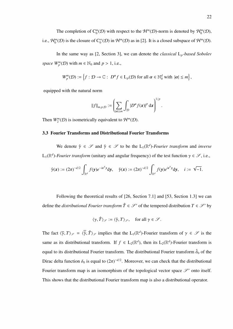
The completion of Cm0 (D) with respect to the Hm(D)-norm is denoted by Hm
0 (D),
i.e.,Hm0 (D) is the closure of C∞0 (D) inHm(D) as in [2]. It is a closed subspace ofHm(D).
In the same way as [2, Section 3], we can denote the classical Lp-based Sobolev
space Wmp (D) with m ∈ N0 and p > 1, i.e.,
Wmp (D) :=
f : D → C : Dα f ∈ Lp(D) for all α ∈ Nd
0 with |α| ≤ m,
equipped with the natural norm
‖ f ‖m,p,D :=
∑|α|≤m
∫D
|Dα f (x)|p dx
1/p
.
Then Wm2 (D) is isometrically equivalent toHm(D).
3.3 Fourier Transforms and Distributional Fourier Transforms
We denote γ ∈ S and γ ∈ S to be the L1(Rd)-Fourier transform and inverse
L1(Rd)-Fourier transform (unitary and angular frequency) of the test function γ ∈ S , i.e.,
γ(x) := (2π)−d/2∫Rd
f (y)e−ixT ydy, γ(x) := (2π)−d/2∫Rd
f (y)eixT ydy, i :=√−1.
Following the theoretical results of [26, Section 7.1] and [53, Section 1.3] we can
define the distributional Fourier transform T ∈ S ′ of the tempered distribution T ∈ S ′ by
〈γ, T 〉S := 〈γ,T 〉S , for all γ ∈ S .
The fact 〈γ,T 〉S = 〈γ, T 〉S implies that the L1(Rd)-Fourier transform of γ ∈ S is the
same as its distributional transform. If f ∈ L2(Rd), then its L2(Rd)-Fourier transform is
equal to its distributional Fourier transform. The distributional Fourier transform δ0 of the
Dirac delta function δ0 is equal to (2π)−d/2. Moreover, we can check that the distributional
Fourier transform map is an isomorphism of the topological vector space S ′ onto itself.
This shows that the distributional Fourier transform map is also a distributional operator.

23
Now we use the special test functions S2m to introduce the generalized Fourier
transforms of order m.
Definition 3.5 ([60, Definition 8.9]). Suppose that Φ ∈ C(Rd)∩SI. A measurable function
Φm ∈ Lloc2 (Rd\0) is called a generalized Fourier transform of Φ if there exists an integer
m ∈ N0 such that ∫Rd
Φ(x)γ(x)dx =
∫Rd
Φm(x)γ(x)dx, for all γ ∈ S2m.
The integer m is called the order of Φm.
If Φ has a generalized Fourier transform of order m, then it has also order l ≥ m,
and its generalized Fourier transform and its distributional Fourier transform coincide on
the set S2m, i.e.,
〈γ, Φ〉S = 〈γ,Φ〉S =
∫Rd
Φ(x)γ(x)dx =
∫Rd
Φm(x)γ(x)dx, for all γ ∈ S2m.
If Φ ∈ L2(Rd)∩C(Rd), then its L2(Rd)-Fourier transform is a generalized Fourier transform
of any order. Even if Φ does not have any generalized Fourier transform, it always has a
distributional Fourier transform Φ since Φ can be seen as a tempered distribution.
Our main goal in this subsection is to define the distributional Fourier transform of
a distributional operator induced by the FT space defined in (3.1).
Definition 3.6. Let P be a distributional operator. If there is a function p ∈ FT such that
〈γ, PT 〉S = 〈γ, pT 〉S = 〈pγ, T 〉S , for all T ∈ S ′ and all γ ∈ S ,
then p is said to be a distributional Fourier transform of P.
Lemma 3.2. If the distributional operator P has the distributional Fourier transform p, then
P is translation-invariant.
Proof. τhPγ(x) = e−ixT h p(x)γ(x) = Pτhγ(x) for all h ∈ Rd and all γ ∈ S .

24
Lemma 3.3. If the distributional operator P is complex-adjoint invariant and has the dis-
tributional Fourier transform p, then p is the distributional Fourier transform of the distri-
butional adjoint operator P∗.
Proof. We can verify that
〈γ, pT 〉S = 〈p ˆγ, T 〉S = 〈Pγ, T 〉S = 〈Pγ,T 〉S = 〈Pγ,T 〉S = 〈γ, P∗T 〉S = 〈γ, P∗T 〉S
for all T ∈ S ′ and all γ ∈ S .
Because of Dαγ =(pγ
)for each γ ∈ S , we can show that any distributional
derivative Dα has the distributional Fourier transform p(x) := (ix)α where i =√−1. This
also implies that the distributional Fourier transform p∗ of its adjoint operator (−1)|α|Dα is
equal to p∗(x) = (−ix)α = p(x). Furthermore, we can also obtain the distributional Fourier
transform of a differential operator (with constant coefficients) in the same way, e.g.,
p(x) =∑|α|≤n
cα(ix)α, where P =∑|α|≤n
cαDα with cα ∈ C, α ∈ Nd0 and n ∈ N0.
3.4 Boundary Operators
In this section we wish to define boundary operators on the L2-based Sobolev spaces
Hm(D), m ∈ N. Since these boundary operators can not be set up in an arbitrary open
bounded domain, we will assume that D is a regular bounded open domain of Rd, e.g., it
satisfies the uniform Cm-regularity condition which implies the strong local Lipschitz con-
dition and the uniform cone condition (see [2, Section 4.1] and [27, Section 12.10]). This
means that D has a regular boundary ∂D = D\D. Moreover ∂D is closed and bounded
which implies that ∂D is compact because the domainD is bounded.
We begin by defining special L2-based spaces restricted to the boundary ∂D as
L2(∂D) :=
f : ∂D → C : f is measurable and∫∂D
| f (x)|2 dS (x) < ∞

25
together with an inner product given by
( f , g)L2(∂D) :=∫∂D
f (x)g(x)dS (x).
Here∫∂D
f (x)dS (x) says that f is integrable on the boundary ∂D and dS is denoted to be
the surface area whenever d ≥ 2. In the special case d = 1 we interpret the restricted space
as
L2(∂D) := f : ∂D = a, b → C ,
and its inner product as
( f , g)L2(∂D) = f (a)g(a) + f (b)g(b),
because the measure at the endpoints is defined as S (a) = S (b) = 1.
The crucial ingredient that allows us to deal with boundary conditions is a trace
mapping which restricts the derivative of an Hm(D) function to the boundary ∂D. More
precisely, for any fixed β ∈ Nd0 with |β| ≤ m − 1, we call Dβ|∂D a trace mapping of the βth
derivative Dβ.
When d = 1 we have D := (a, b) and ∂D := a, b with −∞ < a < b < +∞.
According to the Sobolev embedding theorem (Rellich-Kondrachov theorem) [2, Theo-
rem 6.3],Hm(a, b) is embedded into Cm−1([a, b]). In this special case the trace mapping of
the βth derivative Dβ, Dβ|∂D : Hm(a, b)→ L2(a, b), is well-defined onHm(a, b) via(Dβ|a,b f
)(x) = Dβ f (x), for all f ∈ Hm(a, b) and all x ∈ a, b.
In the case d ≥ 2, according to the boundary trace embedding theorem ([2, Theo-
rem 5.36] and [27, Theorem 12.76]), the trace mapping
Dβ|∂D f := Dβ f |∂D, for all f ∈ Cm(D) ⊂ Hm(D),
can be extended to a bounded linear operator from Hm(D) into L2(∂D), i.e., there is a
positive constant Cβ such that∥∥∥Dβ|∂D f
∥∥∥L2(∂D)
≤ Cβ ‖ f ‖m,D for all f ∈ Hm(D).

26
Remark 3.3. In the references [2, 27] it is further shown that Dβ|∂D is a surjective mapping
from Hm(D) onto Hm−|β|−1/2(∂D) whenever d ≥ 2. However, we will not be concerned
with the spaceHm−|β|−1/2(∂D) in this thesis.
When d = 1 we also denote C(∂D) := f : ∂D = a, b → C. So C(∂D) ⊆ L2(∂D)
for every dimension d ∈ N which implies that bβ Dβ|∂D f := bβ(Dβ|∂D f
)∈ L2(∂D) when
bβ ∈ C(∂D) and f ∈ Hm(D). Furthermore bβ Dβ|∂D is continuous onHm(D).
Definition 3.7. A boundary operator (with non-constant coefficients) B : Hm(D) →
L2(∂D) is well-defined by
B :=∑|β|≤m−1
bβ Dβ|∂D, where bβ ∈ C(∂D), β ∈ Nd0 and m − 1 ∈ N0.
The order of B is given by
O(B) := max|β| : bβ . 0 where β ∈ Nd
0 with |β| ≤ m − 1.
A vector boundary operator B := (B1, · · · , Bn)T is formed using a finite number of bound-
ary operators B1, . . . , Bn and its order is O(B) := max O(B1), . . . ,O(Bn).
Lemma 3.4. If B is a boundary operator (with non-constant coefficients) of order m − 1 as
Definition 3.7, then B is a continuous linear operator fromHm(D) into L2(∂D).

27
CHAPTER 4
CONSTRUCTING CONDITIONALLY POSITIVE DEFINITE FUNCTIONS VIAGREEN FUNCTIONS
In this chapter we use a vector distributional operator P := (P1, · · · , Pn, · · · )T in-
duced by S to set up a generalized Sobolev space HP(Rd) defined on Rd. We also show
the relationship between (full-space) Green functions and conditionally positive definite
functions, which are published in my papers [20, 61]. All the distributional operators are
induced by the test functions S .
4.1 Green Functions on the Whole Space
Definition 4.1. G is the (full-space) Green function of the distributional operator L if G ∈
S ′ satisfies the equation
LG = δ0. (4.1)
Equation (4.1) is to be interpreted in the sense of distributions which means that
〈L∗γ,G〉S = 〈γ, LG〉S = 〈γ, δ0〉S = γ(0) for all γ ∈ S .
According to Theorem 2.2 and [37] we can obtain the following theorem.
Theorem 4.1. Let L be a distributional operator with distributional Fourier transform l.
Suppose that l is positive on Rd \ 0. Further suppose that l−1 ∈ SI and that l(x) =
Θ(‖x‖2m2 ) as ‖x‖2 → 0 for some m ∈ N0. If the (full-space) Green function G ∈ C(Rd) ∩ SI
of L is even, then G is a conditionally positive definite function of order m on Rd and
Gm(x) := (2π)−d/2l(x)−1, x ∈ Rd,
is its generalized Fourier transform of order m. (Here the notation f = Θ(g) means that
there are two positive numbers C1 and C2 such that C1 |g| ≤ | f | ≤ C2 |g|.)
Proof. First we want to prove that Gm is the generalized Fourier transform of order m of
G. Since l−1 ∈ SI and l(x) = Θ(‖x‖2m2 ) as ‖x‖2 → 0 for some m ∈ N0, the product Gmγ is
28
integrable for each γ ∈ S2m. Let G be the distributional Fourier transform of G. If we can
verify that
〈γ, G〉S =
∫Rd
Gm(x)γ(x)dx, for all γ ∈ S2m,
then we are able to conclude that Gm is the generalized Fourier transform of G.
Since l is the distributional Fourier transform of the distributional operator L we
know that l ∈ FT . Thus Dα(l−1
)∈ SI for each α ∈ Nd
0 because of Dα l ∈ SI and
l−1 ∈ SI. If l(0) > 0, then l−1 ∈ FT , which implies that l−1γ ∈ S for each fixed γ ∈ S2m.
Hence
〈γ, G〉S = 〈l−1γ, lG〉S = 〈l−1γ, LG〉S = 〈l−1γ, δ0〉S = 〈l−1γ, (2π)−d/2〉S
=
∫Rd
(2π)−d/2l(x)−1γ(x)dx =
∫Rd
Gm(x)γ(x)dx.
If l(0) = 0, then l−1 does not belong to FT . However, since l ∈ FT is positive on
Rd \ 0 we can find a positive-valued sequence ln∞n=1 ⊂ C∞(Rd) such that
ln(x) =
l(x), ‖x‖2 > n−1,
l(x) + n−1, ‖x‖2 < n−2.
In particular l1 ≡ 1. And then ln∞n=1 ⊂ FT . It further follows that Dαln converges
uniformly to Dαl on Rd for all α ∈ Nd0.
We now fix an arbitrary γ ∈ S2m. Since l−1n γ and l−1γ have absolutely finite in-
tegral, l−1n γ converges to l−1γ in the integral sense. Let γn := l−1
n γ. We can also check
that(lγn
)ˆ converges to γ point wisely which indicates that
∫Rd G(x)
(lγn
)(x)dx converges
to∫Rd G(x)γ(x)dx. Thus we have
〈γ, G〉S = limn→∞〈lγn, G〉S = lim
n→∞〈γn, LG〉S = lim
n→∞〈γn, δ0〉S = lim
n→∞〈γn, (2π)−d/2〉S
= limn→∞
∫Rd
(2π)−d/2ln(x)−1γ(x)dx =
∫Rd
(2π)−d/2 l(x)−1γ(x)dx =
∫Rd
Gm(x)γ(x)dx.

29
Since Gm ∈ C(Rd \ 0) is positive on Rd \ 0 and G ∈ C(Rd) ∩ SI is an even
function, we can use Theorem 2.2 to conclude that G is a conditionally positive definite
function of order m.
Remark 4.1. If L is a differential operator (with constant coefficients), then its distributional
Fourier transform l satisfies the conditions of Theorem 4.1 if and only if l is a polynomial
of the form l(x) := q(x) + a2m ‖x‖2m2 , where a2m > 0 and q is a polynomial of degree greater
than 2m so that it is positive on Rd \ 0, or q ≡ 0.
4.2 Constructing Generalized Sobolev Spaces with Distributional Operators on theWhole Space
Definition 4.2. Consider the vector distributional operator P = (P1, · · · , Pn, · · · )T con-
sisting of countably many distributional operators P j∞j=1. The generalized Sobolev space
induced by P is defined by
HP(Rd) :=
f ∈ Lloc1 (Rd) ∩ SI :
P j f
∞j=1⊆ L2(Rd) and
∞∑j=1
∥∥∥P j f∥∥∥2
L2(Rd)< ∞
and it is equipped with the semi-inner product
( f , g)HP(Rd) := ( f , g)P,Rd :=∞∑j=1
∫Rd
P j f (x)P jg(x)dx.
For example, if we let P j := Dα for any α ∈ Nd0 with |α| ≤ n and the others
be zero operators, then the L2-based Sobolev space Hn(Rd) ≡ HP(Rd) is a special case
of the generalized Sobolev space. If we choose the vector distributional operator P as
in Example 4.4 then HP(Rd) and Hn(Rd) are isomorphic to each other which indicates
that we redefine the Sobolev space for different inner products using the shape parameter
σ > 0. Generalized Sobolev spaces can also become different kinds of Beppo-Levi spaces
with corresponding semi-inner products (see Example 4.3). The reproducing kernel Hilbert
space of the Gaussian kernel will be isometrically equivalent to a generalized Sobolev space
HP(Rd) as well as explained in Example 4.5.

30
Now we discuss the relationship between the generalized Sobolev space and the
native space. In the following theorems of this section we only consider P constructed by a
finite number of distributional operators P1, . . . , Pn which means that P j := 0 when j > n.
If P := (P1, · · · , Pn)T , then the distributional operator
L := P∗T P =
n∑j=1
P∗jP j
is well-defined, where P∗ :=(P∗1, · · · , P
∗n
)Tis the distributional adjoint operator of P as
defined in Definition 3.3. If we suppose that P is complex-adjoint invariant with distri-
butional Fourier transform p = ( p1, · · · , pn)T , then the distributional Fourier transform
p∗ =(p∗1, · · · , p∗n
)Tof its adjoint operator P∗ is equal to p =
(p1, · · · , pn
)Tby Lemma 3.3.
Since
〈γ, P∗jP jT 〉S = 〈γ, p∗j P jT 〉S = 〈 p∗jγ, p jT 〉S = 〈γ, p j p jT 〉S = 〈γ,∣∣∣p j
∣∣∣2 T 〉S
for all T ∈ S ′ and all γ ∈ S , the distributional Fourier transform l of L is given by
l(x) :=n∑
j=1
∣∣∣ p j(x)∣∣∣2 = ‖ p(x)‖22 , x ∈ Rd.
Moreover, since P has a distributional Fourier transform, P is translation invariant by
Lemma 3.2.
We are now ready to state and prove our main theorem about the generalized
Sobolev spaceHP(Rd) induced by a vector distributional operator P := (P1, · · · , Pn)T .
Theorem 4.2. Let P := (P1, · · · , Pn)T be a complex-adjoint invariant vector distributional
operator with vector distributional Fourier transform p := ( p1, · · · , pn)T which is nonzero
on Rd \ 0. Further suppose that x 7→ ‖ p(x)‖−12 ∈ SI and that ‖ p(x)‖2 = Θ(‖x‖m2 ) as
‖x‖2 → 0 for some m ∈ N0. If the (full-space) Green function G ∈ C(Rd)∩SI of L = P∗T P
is chosen so that it is even, then G is a conditionally positive definite function of order m
on Rd and its native spaceNmG (Rd) is a subspace of the generalized Sobolev spaceHP(Rd).

31
Moreover, their semi-inner products are the same on NmG (Rd), i.e.,
( f , g)NmG (Rd) = ( f , g)HP(Rd), for all f , g ∈ Nm
G (Rd) ⊆ HP(Rd).
Proof. By our earlier discussion the distributional Fourier transform l of L is equal to l(x) =
‖ p(x)‖22. Thus l is positive on Rd\0, l−1 ∈ SI and l(x) = Θ(‖x‖2m2 ) as ‖x‖2 → 0. According
to Theorem 4.1, G is a conditionally positive definite function of order m and its generalized
Fourier transform of order m is given by
Gm(x) := (2π)−d/2 l(x)−1 = (2π)−d/2 ‖ p(x)‖−22 , x ∈ Rd.
With the material developed thus far we are able construct its native space NmG (Rd) by
Theorem 2.3.
Next, we fix any f ∈ NmG (Rd). According to Theorem 2.3, the f ∈ C(Rd) ∩ SI
possesses the generalized Fourier transform f of order m/2 and x 7→ f (x) ‖ p(x)‖2 ∈ L2(Rd).
This means that the functions p j f belong to L2(Rd), j = 1, . . . , n. Hence we can define the
functions fP j ∈ L2(Rd) by
fP j := (p j f ) ∈ L2(Rd), j = 1, . . . , n
using the inverse L2(Rd)-Fourier transform.
Since ‖ p(x)‖2 = Θ(‖x‖m2 ) as ‖x‖2 → 0 we have p j(x) = O(‖x‖m2 ) as ‖x‖2 → 0 for
each j = 1, . . . , n. Thus p jγ ∈ Sm for each γ ∈ S . Moreover, since p jγ = p jγ = p∗jγ = P∗jγ
and the generalized and distributional Fourier transforms of f coincide on Sm we have∫Rd
fP j(x)γ(x)dx =
∫Rd
(p j f )(x)γ(x)dx =
∫Rd
(p j f )(x)γ(x)dx
=〈 p jγ, f 〉S = 〈P∗jγ, f 〉S = 〈P∗jγ, f 〉S = 〈P∗jγ, f 〉S = 〈γ, P j f 〉S ,
for all γ ∈ S . This shows that P j f = fP j ∈ L2(Rd). Therefore we know that f ∈ HP(Rd).

32
To establish equality of the semi-inner products we let f , g ∈ NmG (Rd). Then the
Plancherel theorem [53] yields
( f , g)HP(Rd) =
n∑j=1
∫Rd
fP j(x)gP j(x)dx =
n∑j=1
∫Rd
( p j f )(x)( p jg)(x)dx
=
∫Rd
f (x)g(x) ‖ p(x)‖22 dx =
∫Rd
f (x)g(x)l(x)dx
= (2π)−d/2∫Rd
f (x)g(x)Gm(x)
dx = ( f , g)NmG (Rd).
Remark 4.2. If each element of P is just a differential operator (with constant coefficients)
then all coefficients of the differential operators are real numbers because it is complex-
adjoint invariant.
The preceding theorem shows that NmG (Rd) can be isometrically embedded into
HP(Rd). Ideally, NmG (Rd) would be isometrically equivalent to HP(Rd), but this is not true
in general. However, if we impose some additional conditions on HP(Rd), then we can
obtain equality.
Definition 4.3. Let P := (P1, · · · , Pn)T be a vector distributional operator. We say that
the generalized Sobolev space HP(Rd) possesses the S -dense property if for every f ∈
HP(Rd), every compact subset Λ ⊂ Rd and every ε > 0, there exists γ ∈ S ∩HP(Rd) such
that
| f − γ|HP(Rd) < ε and ‖ f − γ‖L∞(Λ) < ε, (4.2)
i.e., there is a sequence γn∞n=1 ⊆ S ∩HP(Rd) so that
| f − γn|HP(Rd) → 0 and ‖ f − γn‖L∞(Λ) → 0, when n→ ∞.
Following the method of the proofs of [60, Theorems 10.41 and 10.43], we can
complete the proofs of the following lemma and theorem.

33
Lemma 4.3. Suppose that P and G satisfy the conditions of Theorem 4.2 and that HP(Rd)
has the S -dense property as stated in Definition 4.3. Assume we are given arbitrary pair-
wise distinct data points x1, · · · , xN ⊂ Rd and scalars λ1, · · · , λN ⊂ C. If we define
fλ :=∑N
k=1 λkG(· − xk), then for every f ∈ HP(Rd) and every x ∈ Rd we have the represen-
tation (f , fλ(x − ·)
)HP(Rd)
=
N∑k=1
λk f (x − xk). (4.3)
Proof. Let us first assume that γ ∈ S ∩HP(Rd). According to Theorem 4.2, fλ ∈ NmG (Rd) ⊆
HP(Rd). Since P is translation invariant and complex-adjoint invariant we have(γ, fλ(x − ·)
)HP(Rd)
=
n∑j=1
∫Rd
P jγ(y)P j,y fλ(x − y)dy =
n∑j=1
∫Rd
P jγ(y)P j,y fλ(x − y)dy
=
n∑j=1
〈P∗jP jγ, fλ(x − ·)〉S =
∫Rd
fλ(y)Lyγ(x − y)dy =
N∑k=1
∫RdλkG(y − xk)Lyγ(x − y)dy
=
N∑k=1
λk〈γ(x − xk − ·), LG〉S =
N∑k=1
λk〈γ(x − xk − ·), δ0〉S =
N∑k=1
λkγ(x − xk).
For a general f ∈ HP(Rd) we fix x ∈ Rd and choose a compact set Λ ⊂ Rd such
that x − xk ∈ Λ for k = 1, . . . ,N. For any ε > 0, there is a γ ∈ S ∩ HP(Rd) which
satisfies Equation (4.2). Then two applications of the triangle inequality show that the
absolute value of the difference in the two sides of Equation (4.3) can be bounded by
ε(∑N
k=1 |λk| + | fλ|HP(Rd)
), which tends to zero as ε → 0.
Theorem 4.4. Suppose that P and G satisfy the conditions of Theorem 4.2. If HP(Rd)
possesses the S -dense property as stated in Definition 4.3, then
NmG (Rd) ≡ HP(Rd).
Proof. By Theorem 4.2 we already know thatNmG (Rd) is contained inHP(Rd) and that their
semi-inner products are the same in the subspaceNmG (Rd). Moreover,Nm
G (Rd) is a complete
subspace ofHP(Rd). So, if we assume thatNmG (Rd) were not the whole spaceHP(Rd), then
there would be an element f ∈ HP(Rd) which is orthogonal to the native space NmG (Rd).

34
Let Q = dim πm−1(Rd) andq1, · · · , qQ
be a Lagrange basis of πm−1(Rd) with respect
to a πm−1(Rd)-unisolvent subsetξ1, · · · , ξQ
⊂ Rd. We make the special choice of the data
sites−x,−ξ1, · · · ,−ξQ
and scalars
1,−q1(x), · · · ,−qQ(x)
and correspondingly define
fλ := G(· + x) −Q∑
k=1
qk(x)G(· + ξk).
Since HP(Rd) has the S -dense property we can use Lemma 4.3 to represent any f ∈
HP(Rd) in the form
f (w + x) =
Q∑k=1
qk(x) f (w + ξk) + ( f , fλ(w − ·))HP(Rd).
Since G is even, we have x 7→ fλ(−x) ∈ NmG (Rd). We now set w = 0. The fact that f is
orthogonal to NmG (Rd) gives us
f (x) =
Q∑k=1
qk(x) f (ξk) + ( f , fλ(−·))HP(Rd) =
Q∑k=1
f (ξk)qk(x).
This shows that f ∈ πm−1(Rd) ⊆ NmG (Rd), and it contradicts our first assumption. It follows
that NmG (Rd) ≡ HP(Rd).
Lemma 4.5. Suppose that P and G satisfy the conditions of Theorem 4.2. Then
HP(Rd) ∩ L2(Rd) ∩ C(Rd) ⊆ NmG (Rd).
Proof. We fix any f ∈ HP(Rd) ∩ L2(Rd) ∩ C(Rd) and suppose that f and P j f , respectively,
are the L2(Rd)-Fourier transforms of f and P j f , j = 1, . . . , n. Using the Plancherel theorem
we obtain∫Rd
( p j f )(x)( p j f )(x)dx =
∫Rd
P j f (x)P j f (x)dx =
∫Rd
P j f (x)P j f (x)dx < ∞.
And therefore, with the help of the proof of Theorem 4.2, we have∫Rd
∣∣∣ f (x)∣∣∣2
Gm(x)dx = (2π)d/2
∫Rd
∣∣∣ f (x)∣∣∣2 l(x)dx = (2π)d/2
∫Rd
∣∣∣ f (x)∣∣∣2 ‖ p(x)‖22 dx
= (2π)d/2n∑
j=1
∫Rd
∣∣∣ f (x) p j(x)∣∣∣2 dx < ∞

35
showing that f/G1/2
m ∈ L2(Rd), where Gm is the generalized Fourier transform of G. And
now, according to Theorem 2.2, f ∈ NmG (Rd).
This says thatHP(Rd)∩L2(Rd)∩C(Rd) can be isometrically embedded intoNmG (Rd).
Moreover, we can get the identity by an additional sufficient condition.
Theorem 4.6. Suppose that P and G satisfy the conditions of Theorem 4.2. If HP(Rd) ⊆
L2(Rd), then G is a positive definite function on Rd and its related reproducing kernel
Hilbert space is isometrically equivalent to the generalized Sobolev space induced by P,
i.e.,
N0G(Rd) ≡ HP(Rd).
Proof. Since G ∈ NmG (Rd) ⊆ HP(Rd) ⊆ L2(Rd), its generalized Fourier transform of any
order is equal to its L2(Rd)-Fourier transform which implies that G ∈ L2(Rd) ∩ L1(Rd). So
x 7→ ‖ p(x)‖−12 ∈ L2(Rd) and ‖ p(x)‖2 = Θ(1) as ‖x‖2 → 0. According to Theorem 4.2, G is
a positive definite function.
We fix any f ∈ HP(Rd) ⊆ L2(Rd). According to the proof of Lemma 4.5, we have
its distributional Fourier transform f ∈ L2(Rd) and
‖ f ‖2HP(Rd) =
n∑j=1
∫Rd
∣∣∣∣P j f (x)∣∣∣∣2 dx =
n∑j=1
∫Rd
∣∣∣p j(x) f (x)∣∣∣2 dx =
∫Rd‖ p(x)‖22
∣∣∣ f (x)∣∣∣2 dx.
This means in particular that f ∈ L1(Rd) because∫Rd
∣∣∣ f (x)∣∣∣ dx ≤
(∫Rd‖ p(x)‖22
∣∣∣ f (x)∣∣∣2)1/2 (∫
Rd‖ p(x)‖−2
2
)1/2
.
Thus, the inverse L1(Rd)-Fourier transform of f is equal to the inverse L2(Rd)-Fourier trans-
form of f which can be identified with f . This implies that f ∈ C(Rd). According to
Theorem 4.2 and Lemma 4.5, we have NmG (Rd) ≡ HP(Rd).
Remark 4.3. As Example 4.2 in Section 4.3 shows, the native spaceNmG (Rd) will not always
be equivalent to the corresponding generalized Sobolev spaceHP(Rd).

36
If P is a vector differential operator (with real constant coefficients), then l(x) =
‖ p(x)‖22 is a real polynomial. If an element of P is an identity operator, then l(x) ≥ 1 for all
x ∈ Rd. Moreover, if l−1 ∈ L1(Rd), then l−1 ∈ L2(Rd) because l−1 ∈ C(Rd). Using its inverse
L1(Rd)-Fourier transform, we have
G(x) := (2π)−d∫Rd
l(x)−1eixT ydy, x ∈ Rd.
and G ∈ C(Rd) ∩ L2(Rd). Since l is even, G is real and even. In this case, we can obtain a
proposition for vector differential operators.
Proposition 4.7. Let P be a vector differential operator (with real constant coefficients)
and p be its distributional Fourier transforms. Suppose that an element of P is an identity
operator and x 7→ ‖ p(x)‖−12 ∈ L2(Rd). Then
G(x) := (2π)−d∫Rd‖ p(x)‖−2
2 eixT ydy, x ∈ Rd,
is a positive definite function on Rd and its related reproducing kernel Hilbert space is
isometrically equivalent to the generalized Sobolev space induced by P, i.e.,
N0G(Rd) ≡ HP(Rd).
Proof. According to the construction of the function G, its L1(Rd)-Fourier transform G is
equal to (2π)−d/2l−1. G is a Green function of L := P∗T P because
〈γ, LG〉S = 〈 ˆγ, LG〉S = 〈γ, LG〉S = 〈γ, lG〉S =
∫Rd
(2π)−d/2γ(x)dx = γ(0).
for all γ ∈ S . According to the above discussions and Theorem 4.6, we can complete the
proof.

37
4.3 Examples
4.3.1 Two-dimensional Examples.
Example 4.1 (Thin Plate Splines). Let P :=(∂2
∂x21,√
2 ∂2
∂x1∂x2, ∂2
∂x22
)Tso that L := P∗T P = ∆2.
It is well-known that the fundamental solution of the Poisson equation on R2 is given by
x 7→ log ‖x‖2, i.e., ∆ log ‖x‖2 = −2πδ. Therefore Equation (4.1) is solved by
G(x) :=1
8π‖x‖22 log ‖x‖2 , x ∈ R2. (4.4)
Since P and G satisfy the conditions of Theorem 4.2 and ‖ p(x)‖2 = ‖x‖22, G is a condi-
tionally positive definite function of order 2. Moreover, according to [60, Theorem 10.40],
we can verify that HP(R2) has the S -dense property. Therefore, N2G(R2) ≡ HP(R2) by
Theorem 4.4. Equation (4.5) is known as the thin plate spline interpolant (see [7, 14, 34]).
The interpolant of this Green function G has the form
s f ,X(x) :=N∑
j=1
c jG(x − x j) + β3x2 + β2x1 + β1, x = (x1, x2) ∈ R2. (4.5)
We consider the Duchon semi-norm mentioned in [14], i.e.,
| f |2D2:=
∫R2
∣∣∣∣∣∣∂2 f (x)∂x2
1
∣∣∣∣∣∣2 + 2
∣∣∣∣∣∣∂2 f (x)∂x1∂x2
∣∣∣∣∣∣2 +
∣∣∣∣∣∣∂2 f (x)∂x2
2
∣∣∣∣∣∣2 dx,
and the Duchon semi-norm space
HD2(R2) :=
f ∈ Lloc
1 (R2) ∩ SI : | f |D2< ∞
.
If we define P as above, then it is easy to check thatHP(R2) ≡ HD2(R2). According to [60,
Theorems 13.1 and 13.2] we can conclude that the Duchon semi-norm space possesses the
same optimality properties as those listed in [14].
The following example shows that the same Green function G can be computed by
different vector distributional operators P. Moreover, it illustrates the fact that the native
space NmG (Rd) may be a proper subspace ofHP(Rd) as mentioned in Remark 4.3.

38
Example 4.2 (Modified Thin Plate Splines). Let P := ∆ and L := P∗T P = ∆2. We find that
the thin plate spline (4.4) is also the Green function of the differential operator L defined
here. The associated interpolant is again of the form (4.5).
We now consider the Laplacian semi-norm
| f |2∆ :=∫R2|∆ f (x)|2 dx,
and the Laplacian semi-norm space
H∆(R2) :=f ∈ Lloc
1 (R2) ∩ SI : | f |∆ < ∞.
It is easy to verify that HP(R2) ≡ H∆(R2). However, it is known that HD2(R2) is a
proper subspace of H∆(R2) since q ∈ H∆(R2) but q < HD2 where q(x) := x1x2. Therefore,
due to Example 4.1, we conclude that
N2G(R2) ≡ HD2(R
2) & H∆(R2) ≡ HP(R2).
Instead of working with the polynomial space π1(R2) which is used to defineN2G(R2),
we can construct a new native space NPG (R2) for G by using another finite-dimensional
space P of C2(R2)∩SI such thatNPG (R2) may be equal to the other subspace ofHP(R2).
First we can verify that the finite-dimensional space P := spanπ1(R2) ∪ q
is a subspace
of the null space of HP(R2). Since π1(R2) ⊂ P and G is a conditionally positive definite
function of order 2, we know that G is also conditionally positive definite with respect to
P . Hence, the new native spaceNPG (R2) with respect to G and P is well-defined (see [60,
Section 10.3]). We can further check that NPG (R2) is a subspace of HP(R2) but it is larger
than N2G(R2), i.e., N2
G(R2) $ NPG (R2) ⊆ HP(R2).
So we can obtain a modification of the thin plate spline interpolant based on P:
sPf ,X(x) :=
N∑j=1
c jG(x − x j) + β4x1x2 + β3x2 + β2x1 + β1, x = (x1, x2) ∈ R2.

39
Conjecture 4.1. Motivated by Example 4.2 we audaciously guess the following extension
of the theorems in Section 4.2: Let P and G satisfy the conditions of Theorem 4.2. If the
subspace P of the null space ofHP(R2) is a finite-dimensional subspace and π1(R2) ⊆P ,
then the new native space NPG (R2) with respect to G and P is a subspace ofHP(R2).
4.3.2 d-dimensional Examples.
Example 4.3 (Polyharmonic Splines). This is a generalization of the earlier Example 4.1.
Let
P :=
∂m
∂xm1, · · · ,
√m!α!
Dα, · · · ,∂m
∂xmd
T
consisting of all(
m!α!
)1/2Dα with α ∈ Nd
0 and |α| = m > d/2. We further denote L := P∗T P =
(−1)m∆m. Then the polyharmonic spline on Rd is the solution of Equation (4.1) (see [5,
Section 6.1.5]), i.e.,
G(x) :=
Γ(d/2−m)
22mπd/2(m−1)! ‖x‖2m−d2 , for d odd,
(−1)m+d/2−1
22m−1πd/2(m−1)!(m−d/2)! ‖x‖2m−d2 log ‖x‖2 , for d even.
We can also check that P and G satisfy the conditions of Theorem 4.2 and that ‖ p(x)‖2 =
‖x‖m2 . Therefore G is a conditionally positive definite function of order m. Furthermore,
according to [60, Theorem 10.40], we can verify that HP(Rd) has the S -dense property.
Therefore, NmG (Rd) ≡ HP(Rd) by Theorem 4.4.
We now consider the Beppo-Levi space of order m on Rd, i.e.,
BLm(Rd) :=f ∈ Lloc
1 (Rd) ∩ SI : Dα f ∈ L2(Rd) for all α ∈ Nd0 with |α| = m
equipped with the semi-inner product
( f , g)BLm(Rd) :=∑|α|=m
m!α!
∫Rd
Dα f (x)Dαg(x)dx.
According to [35], we know that BLm(Rd) ⊆ Lloc1 (Rd) ∩ SI whenever m > d/2. Hence
HP(Rd) ≡ BLm(Rd).

40
By the way, it is well-known that G is also conditionally positive definite of order
l := m − dd/2e + 1 (see [60, Corollary 8.8]). However, the native spaceN lG(Rd) induced by
G and πl−1(Rd) is a proper subspace of NmG (Rd) when d > 1. Therefore
N lG(Rd) $ Nm
G (Rd) ≡ HP(Rd) ≡ BLm(Rd), d > 1.
Remark 4.4. If we have a vector distributional operator P := (P1, · · · , Pn)T whose distribu-
tional Fourier transform satisfies x 7→ ‖ p(x)‖22 ∈ π2m(Rd) and
aαDα : α ∈ Nd
0 with |α| = m⊆
P j : j = 1, . . . , n
, where aα , 0 and m > d/2,
then HP(Rd) ⊆ BLm(Rd). According to the Sobolev inequality [2], there is a positive
constant C such that ‖ f ‖2HP(Rd) ≤ C ‖ f ‖2BLm(Rd) for each f ∈ HP(Rd). This implies that this
generalized Sobolev spaceHP(Rd) also has the S -dense property.
Example 4.4 (Matern Functions). Let P :=(QT
0 , · · · ,QTn
)T, where σ > 0 and
Q j :=
(
n!σ2n−2 j
j!(n− j)!
)1/2∆k, when j = 2k,(
n!σ2n−2 j
j!(n− j)!
)1/2∆k∇, when j = 2k + 1,
k ∈ N0, j = 0, 1, . . . , n, n > d/2.
Here we use ∆0 := I. We further define L := P∗T P = (σ2I − ∆)n.
The Sobolev spline (or Matern function) is known to be the Green function of L (see
[5, Section 6.1.6] and [18, Section 13.2]), i.e.,
G(x) :=21−n−d/2
πd/2Γ(n)σ2n−d(σ ‖x‖2)n−d/2 Kd/2−n (σ ‖x‖2) , x ∈ Rd,
where z 7→ Kν(z) is the modified Bessel function of the second kind of order ν and z 7→ Γ(z)
is the Gamma function. Since P and G satisfy the conditions of Proposition 4.7, G is
positive definite and the associated interpolant s f ,X is the same as the Sobolev spline (or
Matern) interpolant.
Proposition 4.7 also shows that the generalized Sobolev space HP(Rd) is isomet-
rically equivalent to the reproducing kernel Hilbert space N0G(Rd). Since f ∈ HP(Rd) if

41
and only if ∆n/2 f , f ∈ L2(Rd), HP(Rd) and Hn(Rd) are isomorphic (see [2]). Thus we can
determine that
N0G(Rd) ≡ HP(Rd) Hn(Rd).
Moreover, this shows that the classical Sobolev space Hn(Rd) becomes a reproducing
kernel Hilbert space with HP(Rd)-inner product and its reproducing kernel is given by
K(x, y) := G(x − y).
Example 4.5 (Gaussian Functions). The Gaussian kernel K(x, y) := Φ(x− y) derived from
the Gaussian function Φ is very important and popular in the current research fields of
scattered data approximation and machine learning. Therefore knowledge of the native
space of the Gaussian function or the reproducing kernel Hilbert space of the Gaussian
kernel is of significant interest. In this example we will show that the native space of the
Gaussian function is isometrically equivalent to a generalized Sobolev space.
We firstly consider the Gaussian function with shape parameter σ > 0
Φ(x) := π−d/2σde−σ2‖x‖22 , x ∈ Rd.
We know that Φ is a positive definite function and its L1(Rd)-Fourier transform is given by
(see [18, Section 4])
Φ(x) = (2π)−d/2e−‖x‖22/4σ
2, x ∈ Rd.
According to [60, Theorem 10.12], its native space N0Φ
(Rd) ⊆ L2(Rd).
Let P := (QT0 , · · · ,Q
Tn , · · · )
T , where
Qn :=
(
1n!4nσ2n
)1/2∆k, when n = 2k,(
1n!4nσ2n
)1/2∆k∇, when n = 2k + 1,
k ∈ N0.
Here we again use ∆0 := I. Now we will verify that N0Φ
(Rd) is isometrically equivalent to
HP(Rd). Even though we find that P does not satisfy the conditions of Theorem 4.2, we are
still able to use other techniques in order to combine the results of this chapter to complete
the proof.
42
Let Pn :=(QT
0 , · · · ,QTn
)Tand pn be its distributional Fourier transforms for each
n ∈ N. Denote ln(x) =∥∥∥pn(x)
∥∥∥2
2. We choose the Green function Gn to be the inverse
L1(Rd)-Fourier transform of (2π)−d/2l−1n when n > d/2. Therefore Pn and Gn satisfy the
conditions of Proposition 4.7. This tells us that – as in Example 4.4 –HPn(Rd) is equivalent
to the classical Sobolev spaceHn(Rd) for each n ∈ N. Proposition 4.7 further tells us that
NGn(Rd) ≡ HPn(R
d), when n > d/2.
Furthermore, we can verify that
f ∈ HP(Rd) ⇐⇒ f ∈∞
∩n=1HPn(R
d) and supn∈N‖ f ‖HPn (Rd) < ∞,
which implies that ‖ f ‖HPn (Rd) → ‖ f ‖HP(Rd) as n→ ∞.
Let f ∈ N0Φ
(Rd) and f be the L2(Rd)-Fourier transform of f . We can check that
l1(x) ≤ · · · ≤ ln(x) ≤ · · · ≤ (2π)−d/2Φ(x)−1 and ln(x) → (2π)−d/2Φ(x)−1 as n → ∞. Hence,
l1/2n f ∈ L2(Rd) which implies that f ∈ NGn(R
d). According to the Lebesgue monotone
convergence theorem [2] and Proposition 4.7, we have
limn→∞‖ f ‖2
HPn (Rd) = limn→∞‖ f ‖2
NGn (Rd) = limn→∞
∫Rd
∣∣∣ f (x)∣∣∣2 ln(x)dx
=(2π)−d/2∫Rd
∣∣∣ f (x)∣∣∣2
Φ(x)dx = ‖ f ‖2
N0Φ
(Rd) < ∞.
Therefore f ∈ HP(Rd) and ‖ f ‖N0Φ
(Rd) = ‖ f ‖HP(Rd).
On the other hand, we fix any f ∈ HP(Rd). Then f ∈ HPn(Rd) for each n ∈ N. We
again use the Lebesgue monotone convergence theorem and Proposition 4.7 to show that∫Rd
∣∣∣ f (x)∣∣∣2
Φ(x)dx = (2π)d/2 lim
n→∞
∫Rd
∣∣∣ f (x)∣∣∣2 ln(x)dx = (2π)d/2 lim
n→∞‖ f ‖2
NGn (Rd)
=(2π)d/2 limn→∞‖ f ‖2
HPn (Rd) = (2π)d/2 ‖ f ‖2HP(Rd) < ∞,
which establishes that f/Φ1/2 ∈ L2(Rd), and therefore f ∈ N0
Φ(Rd).
43
Summarizing the above discussion, it follows that the reproducing kernel Hilbert
space of the Gaussian function is given by the generalized Sobolev spaceHP(Rd), i.e.,
N0Φ(Rd) ≡ HP(Rd).
Remark 4.5. According to the Sobolev embedding theorem, we also haveHP(Rd) ⊆ C∞b (Rd)
because HP(Rd) ⊆ Hn(Rd) for any n ∈ N, where C∞b (Rd) is the collection of all functions
in C∞(Rd) which, together with all their partial derivatives, are bounded on Rd. However,
HP(Rd) does not contain polynomials. If f ∈ C∞b (Rd) and there is a positive constant C such
that ‖Dα f ‖L∞(Rd) ≤ C |α| for each α ∈ Nd0, then f ∈ HP(Rd) which implies that f ∈ N0
Φ(Rd).
If we allow the test function space to be D , then we can further think of the Gaussian
function Φ as a (full-space) Green function of L := exp(− 14σ2 ∆), i.e., LΦ = δ0 and Φ, δ0 ∈
D ′ which means that 〈Lγ,Φ〉D = 〈γ, LΦ〉D = 〈γ, δ0〉D = γ(0) for all γ ∈ D.
44
CHAPTER 5
CONSTRUCTING POSITIVE DEFINITE KERNELS VIA GREEN KERNELS
In this chapter, we suppose that all functions are restricted to the real field including
the test function space D , L2(D), L2(∂D) and Hm(D) etc. The dual bilinear product and
the distributional adjoint operators are introduced in the same way as in Chapter 3. All the
differential operators and boundary operators are set up with real non-constant coefficients.
Thus we do not need to discuss the conjugate signs to simplify the notations and the proofs.
All the generalized Sobolev spaces and reproducing kernel Hilbert spaces are composed of
real functions defined on a regular open bounded domainD. The complex case can be han-
dled in a very similar way. Moreover, all relevant positive definite kernels are real-valued
and hence their associated function spaces are also real spaces of real-valued functions.
We use a vector differential operator (with real non-constant coefficients cα ∈ C∞(D)
as in Definition 3.4) P =(P1, · · · , Pnp
)Tof order m and a boundary operator (with real non-
constant coefficients bβ ∈ C(∂D) as in Definition 3.7) B =(B1, · · · , Bnb
)T of order m − 1
to set up the real generalized Sobolev spaces defined on D. In the following sections the
generalized Sobolev functions can have homogeneous or nonhomogeneous boundary con-
ditions. In my published paper [21] we only consider the boundary conditions constructed
by a finite dimensional basis. Now we will generalize those theoretical results to an infinite
countable basis.
5.1 Preparations
In the beginning, we give some preparing lemmas about P and B.
5.1.1 Differential Operators. According to Lemma 3.1, the P-semi-inner product is well-
defined onHm(D) via the form
( f , g)P,D :=np∑j=1
∫D
P j f (x)P jg(x)dx, f , g ∈ Hm(Ω).

45
For convenience, we give the new notation
( f , g)D :=∫D
f (x)g(x)dx, when f g is integrable onD,
and
Null(P) := f ∈ Hm(D) : P f = 0 .
When P = ∇ = (∂/∂x1, · · · , ∂/∂xd)T the P-semi-inner product is the same as the
gradient-semi-inner product on the Sobolev space H1(D). The Poincare inequality [27,
Theorem 12.77] states that the gradient-semi-norm is equivalent to theH1(D)-norm on the
spaceH10 (D), i.e., there are two positive constants C1 and C2 such that
C1 ‖ f ‖1,D ≤ | f |∇,D ≤ C2 ‖ f ‖1,D , for all f ∈ H10 (D).
In order to prove a generalized Poincare (Sobolev) inequality for the Sobolev spacesHm(Ω)
we need to set up a special class of vector differential operators.
Definition 5.1. PmD
is defined to be a collection of vector differential operators P =(P1, · · · , Pnp
)Tof order m ∈ N which satisfy the requirements that for each fixed |α| = m
and α ∈ Nd0, there is an element P j(α) ∈
P j
np
j=1such that
P∗j(α)P j(α) = (−1)|α|Dα ρ2α Dα +
n(α)∑k=1
Q∗α,kQα,k, 1 ≤ j(α) ≤ np, n(α) ∈ N0,
where ρα ∈ C∞(D) is positive on the whole domain D and Qα,k, Q∗α,k, k = 1, · · · , n(α), are
differential operators and their distributional adjoint operators. (This indicates minx∈D ρα(x)2 >
0 for all possible α becauseD is compact.)
Let’s consider an example. If d = 2, then both vector differential operators P1 :=

46
(P11, P12, P13)T =
(∂2
∂x21,√
2 ∂2
∂x1∂x2, ∂2
∂x22
)Tand P2 := P21 = ∆ belong to P2
Dbecause
P∗11P11 = Dα 1 Dα, where α = (2, 0),
P∗12P12 = Dα 2 Dα, where α = (1, 1),
P∗13P13 = Dα 1 Dα, where α = (0, 2),
and (using the definitions of P1 j just made)
P∗21P21 = D(2,0) 1 D(2,0) + P∗12P12 + P∗13P13,
P∗21P21 = D(1,1) 2 D(1,1) + P∗11P11 + P∗13P13,
P∗21P21 = D(0,2) 1 D(0,2) + P∗11P11 + P∗12P12.
Therefore we can verify that P∗T1 P1 =∑3
j=1 P∗1 jP1 j = P∗T2 P2 = P∗21P21 = ∆2. However, the
null spaces of P1 and P2 are different, in fact Null(P1) & Null(P2).
The following lemma extends the Poincare inequality from the usual gradient semi-
norm to more general P-semi norms and higher-order Sobolev norms. Since we could not
find it anywhere in the literature we provide a proof.
Lemma 5.1. If P ∈PmD
then there exist two positive constants C1 and C2 such that
C1 ‖ f ‖m,D ≤ | f |P,D ≤ C2 ‖ f ‖m,D , for all f ∈ Hm0 (D). (5.1)
Proof. By the method of induction, we can easily check that the second inequality in (5.1)
is true. We now verify the first inequality in (5.1). Fixing any f ∈ Hm0 (D), there is a
sequence γk∞k=1 ⊂ D so that ‖γk − f ‖m,D → 0 when k → ∞. Because of P ∈Pm
D, for each

47
fixed α ∈ Nd0 with |α| = m, there is an element P j(α) of P such that
∥∥∥P j(α) f∥∥∥2
D=
(P j(α) f , P j(α) f
)D
= limk→∞
(P j(α)γk, P j(α)γk
)D
= limk→∞
(P∗j(α)P j(α)γk, γk
)D
= limk→∞
((−1)|α|Dα ρ2
α Dαγk, γk
)D
+ limk→∞
n(α)∑l=1
(Q∗α,lQα,lγk, γk
)D
= limk→∞
(ρα Dαγk, ρα Dαγk)D + limk→∞
n(α)∑l=1
(Qα,lγk,Qα,lγk
)D
= (ρα Dα f , ρα Dα f )D +
n(α)∑l=1
(Qα,l f ,Qα,l f
)D ≥ ‖ραDα f ‖2D
≥ minx∈D|ρα(x)|2 ‖Dα f ‖2D .
Since the uniformly continuous function ρα is positive in the compact subset D, we have
minx∈D |ρα(x)| > 0. Therefore,
C2P
∑|α|=m
‖Dα f ‖2D ≤ | f |2P,D ,
where C2P := n−d
p minρα(x)2 : x ∈ D, α ∈ Nd
0 with |α| = m> 0. According to the Sobolev
inequality [2, Theorem 4.31], there exists a positive constant CD such that
C2D ‖ f ‖
2m,D ≤
∑|α|=m
‖Dα f ‖2D , for all f ∈ Hm0 (D).
By choosing C1 := CPCD > 0 we complete the proof.
Remark 5.1. Similar as Lax-Milgram theorem of second-order (uniformly) elliptic differ-
ential operators [17, Section 6.2.1], we can generalize PmD
to be a collection of the vector
differential operator P whose related differential operator L := P∗T P has the elliptic char-
acters, i.e.,
L = P∗Tm A Pm + Q∗T Q,
where
Pm :=(∂m
∂xm1, · · · ,Dα, · · · ,
∂m
∂xmd
)T
, P∗m = (−1)m Pm,

48
consisting of all Dα with α ∈ Nd0 and |α| = m, and Q is a vector differential operator of
order no more than m, and A :=(a jk
)n,n
j,kcomposing of a jk ∈ C∞(D) is uniformly positive
definite onD which means that
Cm ‖b‖22 ≤ bT A(x)b, for all b ∈ Rn and all x ∈ D,
where n := dim(Pm) = dm
(m−1+d
d
)and Cm is a positive constant independent on c and x. This
indicates that A(x) is a positive definite matrix for all x ∈ D. It is easy to check that PmD
as in Definition 5.1 is a special case of this generalized collection with elliptic conditions
because A = diag(ρ2α
)|α|=m
. In this generalized case, we can use the similar techniques of
the proof of Lemma 5.1 to verify that
Cm
∑|α|=m
‖Dα f ‖2D = Cm
∫D
Pm f (x)T Pm f (x)dx ≤∫D
Pm f (x)T A(x)Pm f (x)dx
≤
∫D
Pm f (x)T A(x)Pm f (x)dx +
∫D
Q f (x)T Q f (x)dx = | f |2P,D , for all f ∈ Hm0 (D).
Therefore, we can also obtain the same inequality as in (5.1). This means that all theoretical
results and proofs in this chapter are the same even if we generalize PmD
to be the collection
of vector differential operators with elliptic conditions.
5.1.2 Boundary Operators. Using Lemma 3.4 we can give a definition of the B-semi-
inner product onHm(D) via the form
( f , g)B,∂D :=nb∑j=1
∫∂D
B j f (x)B jg(x)dS (x), f , g ∈ Hm(D).
For convenience, we give the new notation
( f , g)∂D :=∫∂D
f (x)g(x)dS (x), when f g is integrable on ∂D.
Given a function f ∈ H1(D), it is well known that f ∈ H10 (D) if and only if f van-
ishes on its boundary trace. Therefore we need sufficiently many homogeneous boundary
conditions to determine whether a function f ∈ Hm(D) belongs toHm0 (D).

49
Definition 5.2. BmD
is defined to be a collection of vector boundary operators B =(B1, · · · , Bnb
)T
of order m − 1 ∈ N0 which satisfy the requirement that
B f = 0 ⇐⇒ Dβ|∂D f = 0 for all β ∈ Nd0 with |β| ≤ m − 1,
when f ∈ Hm(D).
We illustrate Definition 5.2 with some examples for the set B2D
in the case d = 1
with ∂D := 0, 1. Two possible members of B2D
are
B1 =
ddx
∣∣∣∂D
I|∂D
or B2 =
ddx
∣∣∣∂D
+ I|∂D
ddx
∣∣∣∂D− I|∂D
.While these are both first-order vector boundary operators, their B1 and B2-semi-inner
products defined inH2(D) are different.
Because of the trivial (standard) traces theorem [2, Theorem 5.37] we know that
f ∈ Hm0 (D) if and only if Dβ|∂D f = 0 for all β ∈ Nd
0 with |β| ≤ m−1 whenever f ∈ Hm(D).
In analogy to this, we can verify the same trivial trace property for the vector boundary
operators B ∈ BmD
.
Lemma 5.2. If B ∈ BmD
, then f ∈ Hm(D) belongs toHm0 (D) if and only if B f = 0.
5.1.3 Combination of Differential and Boundary Operators. Next we define a differen-
tial operator L computed by P, i.e.,
L = P∗T P =
np∑j=1
P∗jP j.
Here the differential equation L f = g is well-defined in the distributional sense, i.e.,
〈Lγ, f 〉D = 〈γ, L f 〉D = 〈γ, g〉D for all γ ∈ D . We continue to construct homogeneous
differential equations with respect to L and B onHm(D), i.e.,L f = 0, inD,
B f = 0, on ∂D.(5.2)

50
Lemma 5.3. Suppose that P ∈ PmD
and B ∈ BmD
. Equation (5.2) has the unique trivial
solution f ≡ 0 inHm(D).
Proof. It is obvious that f ≡ 0 is a solution of Equation (5.2). Suppose that f ∈ Hm(D) is a
solution of Equation (5.2). Since B ∈ BmD
and B f = 0, Lemma 5.2 tells us that f ∈ Hm0 (D).
Thus there is a sequence γk∞k=1 ⊂ D such that ‖γk − f ‖m,D → 0 when k → ∞. And then,
using the two bilinear forms introduced earlier,np∑j=1
(P j f , P j f
)D
= limk→∞
np∑j=1
(P j f , P jγk
)D
= limk→∞
np∑j=1
〈γk, P∗jP j f 〉D = limk→∞〈γk, L f 〉D = 0.
Since P ∈PmD
, the generalized Sobolev inequality of Lemma 5.1 provides the estimate
‖ f ‖2D ≤ ‖ f ‖2m,D ≤ CP | f |2P,D = CP
np∑j=1
∥∥∥P j f∥∥∥2
D= 0, CP > 0.
This, however, implies that f ≡ 0 is the unique solution of Equation (5.2).
Note that in the above proof we employed both the integral and dual bilinear forms.
Since we can only ensure that P∗jP j f ∈ D ′, this quantity needs to be handled with the
dual bilinear form. On the other hand, P j f ∈ L2(D) implies that we can apply the inte-
gral bilinear form in this case. Using the Riesz representation, we therefore obtain that(P j f , P jγk
)D
= 〈P jγk, P j f 〉D = 〈γk, P∗jP j f 〉D because P jγk ∈ D .
Denote
Null(L) := f ∈ Hm(D) : L f = 0 .
Since Hm(D) is separable [2, Section 3.5], Null(L) with respect to the Hm(D)-norm is
also separable. When d = 1 the equation L f = 0 is an ordinary differential equation which
implies that Null(L) is finite dimensional.
Lemma 5.4. Suppose that P ∈PmD
and B ∈ BmD
. Null(L) is closed inHm(D).
Proof. Let Null(L) be the closure of Null(L) with respect to the Hm(D)-norm. If we can
show that Null(L) = Null(L), then we complete the proof. It is obvious that Null(L) ⊆

51
Null(L) SinceHm(D) is complete,Null(L) ⊆ Hm(D). Because the convergence inHm(D)
implies the convergence in D ′ with the weak-star topology. This shows that Null(L) ⊆
T ∈ D ′ : LT = 0. Thus Null(L) ⊆ Null(L).
Proposition 5.5. Suppose that P ∈PmD
and B ∈ BmD
. Hm0 (D) ⊕ Null(L) = Hm(D).
Proof. According to Lemma 5.4, Hm0 (D) ⊕ Null(L) is a closed subspace inHm(D). Thus
Hm0 (D) ⊕ Null(L) ⊆ Hm(D). Now we want to show that Hm(D) ⊆ Hm
0 (D) ⊕ Null(L).
Since Hm0 (D) is a separable Hilbert space, Hm
0 (D) has an orthonormal basis φk∞k=1. For
any fixed f ∈ Hm(D) we let
fP :=∞∑
k=1
ckφk ∈ Hm0 (D) and fB := f − fP, where ck := ( f , φk)P,D , k ∈ N.
If fB = 0 then fB ∈ Null(L). Suppose that fB , 0. We also know that fB is orthogonal
to Hm0 (D) with respect to the P-semi-inner-product, i.e., ( fB, h)P,D = 0 for all h ∈ Hm
0 (D).
We can determine that fB ∈ Null(L) because
〈γ, L fB〉D =
np∑j=1
〈γ, P∗jP j fB〉D =
np∑j=1
(P j fB, P jγ
)D
= ( fB, γ)P,D = 0, for all γ ∈ D .
SoHm0 (D) ⊕ Null(L) = Hm(D).
Lemma 5.6. Let P and B be differential and boundary operators of orders no more than m
and m−1, respectively. Suppose that f :=∑∞
k=1 ckϕk where the sequences ϕk∞k=1 ⊂ H
m(D)
and ck∞k=1 ⊂ R. If
∑∞k=1 |ck| ‖ϕk‖m,D < ∞, then f ∈ Hm(D). Moreover, P f =
∑∞k=1 ckPϕk
and B f =∑∞
k=1 ckBϕk.
Proof. For all α ∈ Nd0 with |α| ≤ m, we have∫
D
∣∣∣∣∣∣∣∞∑
k=1
ckDαϕk(x)
∣∣∣∣∣∣∣2
dx
1/2
≤
∞∑k=1
|ck| ‖Dαϕk‖D ≤
∞∑k=1
|ck| ‖ϕk‖m,D < ∞.
which implies that f ∈ Hm(D). Since P and B are continuous onHm(D), P f =∑∞
k=1 ckPϕk
and B f =∑∞
k=1 ckBϕk.

52
Lemma 5.7. Let ek∞k=1 be an orthonormal basis of ⊗nb
j=1L2(∂D). If ψk ∈ Hm(D) is a solution
of Equation (5.3) for each k ∈ N, i.e.,Lψk = 0, inD,
Bψk = ek, on ∂D,(5.3)
then ψk∞k=1 is an orthonormal basis of Null(L) with respect to the B-semi-inner product.
Proof. We can confirm that ψk∞k=1 is an orthonormal subset of Null(L) with respect to
the B-semi-inner product because (ψk, ψl)B,∂D = (ek, el)⊗nbj=1L2(∂D) =
∑nbj=1
(ek, j, el, j
)∂D
= δkl,
k, l ∈ N, where δ jk is the Kronecker delta function, i.e., δ jk = 0 when j , k and δ jk = 1
when j = k. To show that ψk∞k=1 is also a basis ofNull(L) with respect to the B-semi-inner
product, we assume that there exists a ϕ ∈ Null(L) orthogonal to ψk∞k=1 with respect to the
B-semi-inner product. Thus (Bϕ, ek)⊗nbj=1L2(∂D) =
∑nbj=1
(B jϕ, B jψk
)∂D
= (ϕ, ψk)B,∂D = 0 for
all k ∈ N which implies that Bϕ = 0. According to Lemma 5.3, ϕ ≡ 0.
5.2 Green Kernels on Bounded Domains
Definition 5.3. Suppose that the set R := Γ(·, y) : y ∈ D ⊆ ⊗nbj=1L2(∂D), where the vector
function Γ = (Γ1, · · · ,Γnb)T defined on ∂D × D consists of elements belonging to the
completion of the tensor product of L2(∂D) and Null(L). A kernel Ψ : D × D → R is
called a Green kernel of L and B with boundary conditions given by R if Ψ(·, y) ∈ Hm(D),
y ∈ D, is a solution of LΨ(·, y) = δy, inD,
BΨ(·, y) = Γ(·, y), on ∂D.
If R ≡ 0, then the kernel G : D × D → R is called a Green kernel of L and B with
homogeneous boundary conditions, i.e., G(·, y) ∈ Hm(D), y ∈ D, is a solution ofLG(·, y) = δy, inD,
BG(·, y) = 0, on ∂D.

53
Remark 5.2. We can also use Lemma 5.3 to verify that the Green kernel, provided it exists,
is a unique solution for any given set of boundary conditions Γ. However, for some bound-
ary conditions Γ there may be no solution because the trace mapping is not a surjective
map.
Next we will view the relationship between the eigenvalues and eigenfunctions of
the Green kernels (reproducing kernels) and those of the differential operators with either
homogeneous or nonhomogeneous boundary conditions.
Definition 5.4. Let Ψ ∈ L2(D × D). Real scalarsλp
∞p=1
and nontrivial L2(D)-functionsep
∞p=1
are called eigenvalues and eigenfunctions of Ψ if, for all p ∈ N,
(IΦ,Dep
)(y) =
(Ψ(·, y), ep
)D
= λpep(y), y ∈ D,
where IΦ,D is the integral operator defined in (2.3).
Definition 5.5. Let the set E :=ηp
∞p=1⊆ ⊗
nbj=1L2(∂D). Real scalars
µp
∞p=1
and non-
trivialHm(D)-functionsep
∞p=1
are called eigenvalues and eigenfunctions of L and B with
boundary conditions given by E if, for all p ∈ N, we haveLep = µpep, inD,
Bep = ηp, on ∂D.
If E ≡ 0, then the real scalarsµp
∞p=1
and nontrivial Hm(D)-functionsep
∞p=1
are called
eigenvalues and eigenfunctions of L and B with homogeneous boundary conditions, i.e.,
for all p ∈ N, we have Lep = µpep, inD,
Bep = 0, on ∂D.
The reader may be wondering about our use of different names for Green kernels.
In the following we will use these different names to distinguish between various types of

54
Green kernels. The kernels G (which is now a kernel in this chapter) and K are defined in
Theorems 5.9 and 5.18, and they are Green kernels with homogeneous and nonhomoge-
neous boundary conditions, respectively. Moreover, we introduce a kernel R determined by
the set A defined in Lemma 5.15. We will verify below that K, G and R are reproducing
kernels. Finally, we use the symbol Ψ to denote the Green kernel corresponding to the
general boundary conditions stated in Definition 5.3. The Green kernel Ψ may not be a
reproducing kernel. An example of such a typical case is given in Remark 5.6.
5.3 Constructing Generalized Sobolev Spaces with Differential Operators and Bound-ary Operators on Bounded Domains
In this section, we suppose that P ∈ PmD
and B ∈ BmD
where m > d/2. Then
L = P∗T P is a differential operator of order 2m.
5.3.1 Homogeneous Boundary Conditions.
Definition 5.6. Define the real generalized Sobolev space with homogeneous boundary
conditions induced by P and B via the form
H0P(D) := f ∈ Hm(D) : B f = 0 = Null(B),
and it is equipped with the inner product
( f , g)H0P(D) := ( f , g)P,D.
We now show that the H0P(D)-inner product is well-defined. If f ∈ H0
P(D) such
that | f |P,D = 0, then B f = 0 and∥∥∥P j f
∥∥∥D
= 0, j = 1, · · · , np, which implies that
〈γ, L f 〉D =
np∑j=1
〈γ, P∗jP j f 〉D =
np∑j=1
(P j f , P jγ
)D
=
np∑j=1
(0, P jγ
)D
= 0, for all γ ∈ D.
Thus f solves Equation (5.2) and then Lemma 5.3 states that f = 0.
Theorem 5.8. H0P(D) and Hm
0 (D) are isomorphic, and therefore H0P(D) is a separable
Hilbert space.

55
Proof. According to Lemma 5.2, H0P(D) = Hm
0 (D). The generalized Poincare (Sobolev)
inequality of Lemma 5.1 further shows that the H0P(D)-norm and the Hm(D)-norm are
isomorphic onHm0 (D).
Theorem 5.9. Suppose that there exists a Green kernel G of L and B with homogeneous
boundary conditions. Then H0P(D) is a reproducing kernel Hilbert space with the repro-
ducing kernel G.
Proof. According to Theorem 5.8, H0P(D) Hm
0 (D). Fix any y ∈ D. Since G(·, y) ∈
Hm(D) and BG(·, y) = 0, we have G(·, y) ∈ Hm0 (D) by Lemma 5.2.
We now verify the reproduction property of G. According to the Sobolev embed-
ding theorem [2], Hm(D) is embedded into C(D) when m > d/2, i.e., there is a positive
constant Cm such that
‖ f ‖C(D) := sup | f (x)| : x ∈ D ≤ Cm ‖ f ‖m,D , f ∈ Hm(D) ⊆ C(D).
For any fixed f ∈ H0P(D) there is a sequence γk
∞k=1 ⊂ D such that
| f (y) − γk(y)| ≤ ‖ f − γk‖C(D) ≤ Cm ‖ f − γk‖m,D → 0, when k → ∞. (5.4)
Since
(γk,G(·, y))P,D =
np∑j=1
(P jγk, P jG(·, y)
)D
=
np∑j=1
〈P jγk, P jG(·, y)〉D
=
np∑j=1
〈γk, P∗jP jG(·, y)〉D = 〈γk, LG(·, y)〉D = 〈γk, δy〉D = γk(y), for all k ∈ N,
we can determine that∣∣∣( f ,G(·, y))P,D − γk(y)∣∣∣ =
∣∣∣( f ,G(·, y))P,D − (γk,G(·, y))P,D
∣∣∣≤ ‖ f − γk‖P,D ‖G(·, y)‖P,D ≤ CP ‖ f − γk‖m,D ‖G(·, y)‖m,D → 0, when k → ∞,
(5.5)
where the positive constant CP is independent of the function f . Here – as before – the
two notations (·, ·)D and 〈·, ·〉D denote the integral bilinear form and the dual bilinear form,

56
respectively. Combining Equations (5.4) and (5.5), we will get
( f ,G(·, y))H0P(D) = ( f ,G(·, y))P,D = f (y).
Remark 5.3. As discussed in Remark 5.6, the homogeneous Green kernel of L and B always
exists provided we can find the Green kernel of L and B for some boundary conditions.
Corollary 5.10. The homogeneous Green kernel G of L and B is a symmetric positive
definite kernel onD.
Proof. Fix any set of distinct points X = x1, · · · , xN ⊂ D and coefficients c ∈ RN , N ∈ N.
Since G is the reproducing kernel of the reproducing kernel Hilbert space H0P(D), G is
symmetric and positive semi-definite, i.e.,
N∑j=1
N∑k=1
c jckG(x j, xk) =
N∑j=1
c jG(·, x j),N∑
k=1
ckG(·, xk)
P,D
=
∥∥∥∥∥∥∥N∑
j=1
c jG(·, x j)
∥∥∥∥∥∥∥2
P,D
≥ 0.
To get strict positive definiteness we assume∑N
j=1 c jG(·, x j) = 0. For any γ ∈ D ,
N∑j=1
c jγ(x j) =
N∑j=1
c j〈γ, δx j〉D =
N∑j=1
c j〈γ, LG(·, x j)〉D =
γ, N∑j=1
c jG(·, x j)
P,D
= 0.
To show that c j = 0, j = 1, · · · ,N, we pick an arbitrary x j ∈ X and construct γ j ∈ D such
that γ j vanishes on X\x j, but γ j(x j) , 0. Therefore
N∑j=1
N∑k=1
c jckG(x j, xk) > 0, when c , 0.
Since G(·, y) ∈ C(D) for each y ∈ D, G is uniformly continuous on D which
implies that G ∈ L2(D×D). According to Mercer’s theorem, there is an orthonormal basis
ep∞p=1 of L2(D) and a positive sequence λp
∞p=1 such that G(x, y) =
∑∞p=1 λpep(x)ep(y) and

57
(G(·, y), ep
)D
= λpep(y) for all x, y ∈ D and p ∈ N. According to Proposition 2.5, we
can use the technology of the proof of [60, Proposition 10.29] to verify √
λpep
∞p=1
is an
orthonormal basis of H0P(D). (First we show that
√λpep
∞p=1
is an orthonormal subset of
H0P(D), and then we establish its completeness.)
Proposition 5.11. If positive scalarsλp
∞p=1
and nontrivial L2(D)-functionsep
∞p=1
are
the eigenvalues and eigenfunctions of the homogeneous Green kernel G of L and B, thenλ−1
p
∞p=1
andep
∞p=1
are the eigenvalues and eigenfunctions of L and B with homogeneous
boundary conditions. Moreover, √
λpep
∞p=1
is an orthonormal basis of H0P(D) whenever
ep
∞p=1
is an orthonormal basis of L2(D).
Proof. According to Fubini’s theorem [27, Theorem 12.41], for all p ∈ N and all γ ∈ D ,
〈γ, Lep〉D =(ep, L∗γ
)D
=
∫D
ep(y)(L∗γ)(y)dy
=
∫D
λ−1p
(G(·, y), ep
)D
(L∗γ)(y)dy =
∫D
∫D
λ−1p G(x, y)ep(x) (L∗γ) (y)dxdy
=
∫D
λ−1p ep(x) (G(x, ·), L∗γ)D dx =
∫D
λ−1p ep(x)〈L∗γ,G(·, x)〉Ddx
=
∫D
λ−1p ep(x)〈γ, LG(·, x)〉Ddx =
∫D
λ−1p ep(x)〈γ, δx〉Ddx
=
∫D
λ−1p ep(x)γ(x)dx = 〈γ, λ−1
p ep〉D .
This shows that Lep = λ−1p ep.
According to Proposition 2.5, the integral operator IG,D is a continuous map from
L2(D) intoH0P(D). Since λpep(y) =
(G(·, y), ep
)D
=(IG,Dep
)(y), y ∈ D, we can conclude
that ep ∈ H0P(D). This implies that Bep = 0, p ∈ N. Therefore
λ−1
p
∞p=1
andep
∞p=1
are the
eigenvalues and eigenfunctions of L and B with homogeneous boundary conditions.
Proposition 5.12. If positive scalarsµp
∞p=1
and nontrivial Hm(D)-functionsep
∞p=1
are
the eigenvalues and eigenfunctions of L and B with homogeneous boundary conditions,
thenµ−1
p
∞p=1
andep
∞p=1
are the eigenvalues and eigenfunctions of the homogeneous Green

58
kernel G of L and B. Moreover, ifep
∞p=1
is an orthonormal basis of L2(D), then
G(x, y) =
∞∑p=1
µ−1p ep(x)ep(y), x, y ∈ D.
Proof. We fix y ∈ D and p ∈ N. According to Theorem 5.9 G is a reproducing kernel, i.e.,
we have (G(·, y), ep
)H0
P(D)= ep(y).
Since G(·, y), ep ∈ Hm0 (Ω), we can use the same method as in Lemma 5.1 to verify that
(ep,G(·, y)
)H0
P(D)=
np∑j=1
(P jep, P jG(·, y)
)D
= limk→∞〈γk, Lep〉D =
(µpep,G(·, y)
)D,
where γk∞k=1 ⊂ D satisfy that ‖γk −G(·, y)‖m,D → 0 when k → ∞. Combining the above
equations, we can easily verify that(G(·, y), ep
)D
= µ−1p ep(y). The second claim follows
immediately.
5.3.2 Nonhomogeneous Boundary Conditions. We extend the finite dimensional basis
of Null(L) [21] into the infinitely countable basis of Null(L) to construct the nonhomoge-
neous boundary conditions.
Theorem 5.18 and Corollary 5.17 allow us to arrive at a special theorem.
Theorem 5.13. Suppose that there exists a homogeneous Green kernel G of L and B and
that Null(P) is finite dimensional. Then the real generalized Sobolev space
HAPB(D) = f = fP + fB : B fP = 0 and P fB = 0 where fP, fB ∈ H
m(D) ,
equipped with the inner product
( f , g)HAPB (D) = ( f , g)P,D + ( f , g)B,∂D,
is a reproducing kernel Hilbert space with a reproducing kernel
K(x, y) = G(x, y) +
mb∑k=1
ψk(x)ψk(y), x, y ∈ D,

59
where ψkmbk=1 is an orthonormal basis ofNull(P) with respect to the B-semi-inner product.
Moreover, the reproducing kernel K is a Green kernel of L and B.
Now we will show how to introduce the beautiful theoretical structures.
Definition 5.7. If sequences ψk∞k=1 ⊂ H
m(D) and ak∞k=1 ⊂ R
+0 are such that
∑ak>0
ak ‖ψk‖2m,Ω =
∞∑k=1
ak ‖ψk‖2m,Ω < ∞,
then we say that A := ψk; ak∞k=1 satisfiesHm(D)-Sobolev-embedding conditions.
Similar to solving nonhomogeneous partial differential equations, we want to dis-
cuss the boundary conditions in Null(L). According to Lemma 5.3, Null(L) becomes an
inner-product space when it is given the B-semi-inner product. It is also separable because
the boundary operators are continuous on Hm(D) and Null(L) is closed in the separable
Hm(D) by Lemma 5.4. So it has a countable orthonormal basis ψk∞k=1 ⊂ Null(L), i.e.,(
ψ j, ψk
)B,∂D
= δ jk where δ jk is the Kronecker delta function. However, the completion of
this normable space may not be embedded intoHm(D). Here we want to construct another
Hilbert space which is a subspace of Null(L) and is embedded intoHm(D).
Definition 5.8. We choose an orthonormal basis ψk∞k=1 of Null(L) with respect to the B-
semi-inner product and a nonnegative sequence ak∞k=1 such that the set A := ψk; ak
∞k=1
satisfies theHm(D)-Sobolev-embedding conditions as Definition 5.7. Denote
HAB (D) =
f ∈ Null(L) :∑ak>0
∣∣∣ fk
∣∣∣2ak
< ∞ where fk := ( f , ψk)B,∂D for all k ∈ N
,and it is equipped with the inner-product
( f , g)HAB (D) :=
∑ak>0
1ak
( f , ψk)B,∂D (g, ψk)B,∂D .
In particular, if ak∞k=1 is the zero sequence thenHA
B (D) := 0 and (0, 0)HAB (D) := 0.

60
Lemma 5.14. HAB (D) is a separable Hilbert space. Moreover, there are two positive con-
stants C1 and C2 such that
C1 | f |B,∂D ≤ ‖ f ‖m,D ≤ C2 ‖ f ‖HAB (D) , for all f ∈ HA
B (D) ⊆ Null(L) ⊆ Hm(D).
Proof. If ak∞k=1 contains only a finite number of positive terms, then HA
B (D) is a finite-
dimensional space. Thus the claims of this lemma are obviously true.
Next we assume that ak∞k=1 is a positive sequence. Given any sequence
bk
∞k=1
with∑∞k=1
∣∣∣bk
∣∣∣2 < ∞, if we can show that f =∑∞
k=1 bk√
akψk ∈ HAB (D), thenHA
B (D) is a separa-
ble Hilbert space. Let fn :=∑n
k=1 bk√
akψk. Thus fn ∈ Hm(D) and L fn =
∑nk=1 bk
√akLψk =
0 which implies that fn ∈ Null(L) for all n ∈ N. According to Lemma 5.6, f ∈ Hm(D) and
‖ f − fn‖m,D → 0 when n→ ∞ because
∞∑k=1
∣∣∣bk
∣∣∣ ∥∥∥√akψk
∥∥∥m,D≤
∞∑k=1
∣∣∣bk
∣∣∣21/2 ∞∑k=1
ak ‖ψk‖2m,D
1/2
< ∞.
Lemma 5.4 states that Null(L) is closed inHm(D). So f ∈ Null(L).
We fix any f ∈ HAB (D). For all α ∈ Nd
0 with |α| ≤ m, we have Dα f =∑∞
k=1 fkDαψk
because∞∑
k=1
∣∣∣ fk
∣∣∣ ‖ψk‖m,D ≤
∞∑k=1
∣∣∣ fk
∣∣∣2ak
1/2 ∞∑
k=1
ak ‖ψk‖2m,D
1/2
< ∞.
Lemma 5.6 shows that
‖Dα f ‖D =
∥∥∥∥∥∥∥∞∑
k=1
fkDαψk
∥∥∥∥∥∥∥D
≤
∞∑k=1
∣∣∣ fk
∣∣∣2ak
1/2 ∞∑
k=1
ak ‖Dαψk‖Ω
1/2
.
This implies that
‖ f ‖m,D ≤
(m + 1)d∞∑
k=1
ak ‖ψk‖2m,D
1/2
‖ f ‖HAB (D) .
ThereforeHAB (D) is embedded intoHm(D).
In all the other cases, we pick all the positive elements akn from the nonnegative
sequence ak∞k=1 to compose a new positive sequence
akn
∞n=1. Replacing ψk; ak
∞k=1 by
ψkn; akn
∞n=1, we can complete the proof using in the same technique.

61
Remark 5.4. We can also treat the boundary operator B ∈ BmD
as a bounded linear oper-
ator IB : Hm(D) → Hm−1(∂D) whenever d ≥ 2. Then the B-semi-norm of f ∈ Hm(D)
can be computed by a norm of IB( f ) which is equivalent to the Hm−1(∂D)-norm. Sim-
ilar to the comments made in Remark 3.3, IB is further a surjective map from Hm(D)
onto Hm−1/2(∂D). According to the open mapping theorem [27, Theorem 5.23] and the
first isomorphism theorem for Banach spaces [39, Theorem 1.7.14], we can verify that
Hm−1/2(∂D) Null(L) with respect to the Hm(D)-norm. Since Hm−1/2(∂D) is embedded
intoHm−1(∂D), we can determine that there is a set A as specified in Definition 5.8 so that
HAB (D) Null(L) with respect to theHm(D)-norm.
Lemma 5.15. HAB (D) is a reproducing kernel Hilbert space with a reproducing kernel
R(x, y) :=∑ak>0
akψk(x)ψk(y) =
∞∑k=1
akψk(x)ψk(y), x, y ∈ D.
In particular, when ak∞k=1 is the zero sequence then R := 0.
Proof. We fix any y ∈ D. Since Hm(D) is embedded into C(D) when m > d/2, there is a
positive constant Cm such that
∑ak>0
|akψk(y)|2
ak≤
∑ak>0
ak supx∈D|ψk(x)|2 =
∑ak>0
ak ‖ψk‖2C(D)≤ Cm
∑ak>0
ak ‖ψk‖2m,D < ∞,
which implies that R(·, y) =∑
ak>0 (akψk(y))ψk ∈ HAB (D).
We now turn to the reproduction. For any f =∑
ak>0 fkψk ∈ HAB (D), we have
( f ,R(·, y))HAB (D) =
∑ak>0
fkakψk(y)ak
=∑ak>0
fkψk(y) = f (y).
Since HAB (D) is embedded into Hm(D) by Lemma 5.14, we can determine that
R ∈ C(D×D) and ψk∞k=1 ⊂ C(D).

62
Definition 5.9. Let the set A be chosen in Definition 5.8. We define a real generalized
Sobolev space with nonhomogeneous boundary conditions induced by P, B and A to be a
direct sum space
HAPB(D) := H0
P(D) ⊕HAB (D),
and it is equipped with the inner product
( f , g)HAPB (D) := ( fP, gP)H0
P(D) + ( fB, gB)HAB (D) ,
where fP, gP ∈ H0P(D) and fB, gB ∈ H
AB (D) are the unique decompositions of f , g, i.e.,
f = fP + fB, g = gP + gB, where fP, gP ∈ H0P(D) and fB, gB ∈ H
AB (D).
The direct sum spaceHAPB(D) is well-defined becauseHA
B (D) ⊆ Null(L).
Theorem 5.16. HAPB(D) is a separable Hilbert space and it is embedded intoHm(Ω). More-
over,
( f , g)HAPB (D) = ( f , g)P,D +
∑ak>0
fkgk
ak−
∑ak>0
∑al>0
fkgl(ψk, ψl)P,D, for all f , g ∈ HAPB(D),
where
fk := ( f , ψk)B,∂D and gk := (g, ψk)B,∂D , for all k ∈ N.
In particular, if the set A = ψk; ak∞k=1 further satisfies
ψk : ak > 0, k ∈ N ⊆ Null(P),
then
( f , g)2HA
PB (D) = ( f , g)2P,D +
∑ak>0
fkgk
ak, for all f , g ∈ HA
PB(D).
Proof. According to Theorem 5.8 and Lemma 5.14, we can immediately verify thatHAPB(D)
is a separable Hilbert space and that it is embedded intoHm(D).

63
Fix any f = fP + fB ∈ HAPB(D) where fP ∈ H
0P(D) and fB ∈ H
AB (D). We have
B fP = 0 and L fB = 0. Because of fP ∈ Hm0 (Ω), there is a sequence γk
∞k=1 ⊂ D such that
‖γk − fP‖m,D → 0 when k → ∞. Thus
( fB, fP)P,D = limk→∞
np∑j=1
(P j fB, P jγk
)D
= limk→∞
np∑j=1
〈P jγk, P j fB〉D
= limk→∞
np∑j=1
〈γk, P∗jP j fB〉D = limk→∞〈γk, L fB〉D = 0.
Since B f = B fP + B fB = B fB, we can compute the Fourier coefficients of f as fk =
( f , ψk)B,∂D = ( fB, ψk)B,∂D which implies that fB =∑
ak>0 fkψk and ‖ fB‖2HA
B (D) =∑
ak>0 a−1k
∣∣∣ fk
∣∣∣2.
According to Lemma 5.6, we can verify that P j fB =∑
ak>0 fkP jψk for all j = 1, . . . , np, and
this expansion of P j fB is convergent with respect to the L2(D)-norm. Therefore
( fB, fB)P,D =
np∑j=1
(P j fB, P j fB
)D
=∑ak>0
∑al>0
fk fl
np∑j=1
(P jψk, P jψl
)D,
and
( f , f )P,D = ( fP, fP)P,D + 2 ( fP, fB)P,D + ( fB, fB)P,D = ( fP, fP)P,D +∑ak>0
∑al>0
fk fl (ψk, ψl)P,D .
Summarizing the above discussions, we obtain that
‖ f ‖2HA
PB (D) = ‖ fP‖2H0
P(D) + ‖ fB‖2HA
B (D) = | f |2P,D +∑ak>0
∣∣∣ fk
∣∣∣2ak−
∑ak>0
∑al>0
fk fl (ψk, ψl)P,D .
Remark 5.5. Combining the results of Theorem 5.8 and Remark 5.4, we can also show that
there is a set A as specified in Definition 5.9 so thatHAPB(D) Hm(Ω).
IfNull(P) is a finite-dimensional space, then there is a finite orthonormal set ψkmbk=1
of Null(L) with respect to the B-semi-inner product such that span ψk : k = 1, · · · ,mb =
Null(P). We can extend this orthonormal set to become an orthonormal basis ψk∞k=1 of
Null(L) with respect to the B-semi-inner product, and choose a nonnegative sequence as
a1 = · · · = amb = 1 and amb+1 = · · · = 0 to give us a set A = ψk; ak∞k=1 as specified in
Definition 5.8. Therefore we can formulate the following corollary.

64
Corollary 5.17. If Null(P) is finite-dimensional, then there is a set A as specified in
Definition 5.8 such that
HAPB(D) = Hm
0 (D) ⊕ Null(P)
and its inner product is equal to
( f , g)HAPB (D) = ( f , g)P,D + ( f , g)B,∂D, for all f , g ∈ HA
PB(D).
Moreover,HAPB(D) is isomorphically embedded intoHm(D).
Our main theorem now follows directly from Theorems 5.9 and Lemma 5.15.
Theorem 5.18. Suppose that the kernels G and R are given in Theorem 5.9 and Lemma 5.15.
Then the generalized Sobolev space HAPB(D) is a reproducing kernel Hilbert space with a
reproducing kernel
K(x, y) := G(x, y) + R(x, y), x, y ∈ D.
Moreover, K is a Green kernel of L and B with boundary conditions given by R :=
BR(·, y) : y ∈ D.
By Corollary 5.10 we know that G is a symmetric positive definite kernel, and using
similar arguments we can check that R is symmetric positive semi-definite. Together, this
allows us to formulate the following corollary.
Corollary 5.19. The Green kernel K of L and B defined in Theorem 5.18 is a symmetric
positive definite kernel onD.
Remark 5.6. To see that not every Green kernel is a reproducing kernel, assume that Ψ is a
Green kernel of L and B. Then, according to Proposition 5.5, Ψ can be uniquely written in
the form
Ψ(x, y) = ΨP(x, y) + ΨB(x, y), where ΨP(·, y) ∈ Hm0 (D) and ΦB(·, y) ∈ Null(L).
65
Therefore we haveLΨP(·, y) = δy, inD,
BΨP(·, y) = 0, on ∂D,and
LΨB(·, y) = 0, inD,
BΨB(·, y) = BΨ(·, y), on ∂D.
This means that ΨP is a homogeneous Green kernel of L and B. However, there may not
be any set A such that R = ΨB. This shows that Ψ may not be a reproducing kernel of a
reproducing kernel Hilbert space. For example, Ψ(x, y) := −12 |x − y| is the Green kernel of
L := −d2/dx2. However, Φ(x) := Ψ(x, 0) is only a conditionally positive definite function
of order one and therefore cannot be a reproducing kernel.
We are now ready to address nonhomogeneous boundary conditions. Consider a
kernel Γ ∈ L2(∂D ×D). Then we can define an integral operator IΓ,D : L2(D) → L2(∂D)
via the form
(IΓ,D f
)(x) := (Γ(x, ·), f )D , for all f ∈ L2(D) and x ∈ ∂D.
Let Γ denote the vector function Γ(·, y) =(Γ1(·, y), · · · ,Γnb(·, y)
)T := BK(·, y) for
any y ∈ D, i.e., Γ j(·, y) = B jK(·, y), j = 1, . . . , nb. Since B jG(·, y) = 0 and R(·, y) ∈ Hm(D)
for all y ∈ D, we have
Γ j(·, y) = B jK(·, y) = B jG(·, y) + B jR(·, y) = B jR(·, y) =
∞∑k=1
ak
(B jψk
)ψk(y).
As a consequence we have Γ j ∈ L2(∂D×D).
Proposition 5.20. If positive scalarsλp
∞p=1
and nontrivial L2(D)-functionsep
∞p=1
are the
eigenvalues and eigenfunctions of the Green kernel K of L and B defined in Theorem 5.18,
thenλ−1
p
∞p=1
andep
∞p=1
are the eigenvalues and eigenfunctions of L and B with boundary
conditions given by
E :=ηp :=
(λ−1
p IΓ1,Dep, · · · , λ−1p IΓnb ,D
ep
)T∞
p=1,

66
i.e., ηp, j(x) = λ−1p
(Γ j(x, ·), ep
)D
for all x ∈ ∂D. Here Γ(·, y) := BK(·, y) for any y ∈
∂D. Moreover, √
λpep
∞p=1
is an orthonormal basis of HAPB(D) whenever
ep
∞p=1
is an
orthonormal basis of L2(D).
Proof. Using the same method as in the proof of Proposition 5.11, we can verify that
〈γ, Lep〉D = 〈γ, λ−1p ep〉D for all γ ∈ D . This implies that Lep = λ−1
p ep for all p ∈ N.
Next we compute their boundary conditions. Fix any boundary operator B j, j =
1, · · · , nb, and any eigenfunction ep and eigenvalue λp of K, p ∈ N. Since K ∈ C(D × D)
is positive definite, Mercer’s theorem ensures the existence of an orthonormal basis ϕk∞k=1
of L2(D) and a positive sequence νk∞k=1 such that K(x, y) =
∑∞k=1 νkϕk(x)ϕk(y), x, y ∈ D.
We can also check that√νkϕk
∞k=1
is an orthonormal basis of HAPB(D). Let Kn(x, y) :=∑n
k=1 νkϕk(x)ϕk(y) for any n ∈ N. Thus ‖K(·, y) − Kn(·, y)‖2HA
PB (D) =∑∞
k=n+1 νk |ϕk(y)|2 → 0
when n → ∞. According to Theorem 5.16, HAPB(D) is embedded into Hm(D), which
implies that ‖K(·, y) − Kn(·, y)‖m,D → 0 when n → ∞. So B jK(·, y) =∑∞
k=1 νk
(B jϕk
)ϕk(y)
and(B j,xK(x, ·), ep
)D
=∑∞
k=1 νk
(B jϕk
)(x)
(ϕk, ep
)D
. This shows that
λp
(B jep
)(x) = B j,x
(K(x, ·), ep
)D
=(B j,xK(x, ·), ep
)D
=(Γ j(x, ·), ep
)D, x ∈ ∂D.
It follows that the boundary conditions have the form Bep = ηp for all p ∈ N.
Proposition 5.21. If positive scalarsµp
∞p=1
and nontrivial Hm(D)-functionsep
∞p=1
are
the eigenvalues and eigenfunctions of L and B with boundary conditions given by
E :=ηp :=
(µpIΓ1,Dep, · · · , µpIΓnb ,D
ep
)T∞
p=1,
i.e., ηp, j(x) = µp
(Γ j(x, ·), ep
)D
for all x ∈ ∂D, thenµ−1
p
∞p=1
andep
∞p=1
are the eigenval-
ues and eigenfunctions of the Green kernel K of L and B defined in Theorem 5.18. Here
Γ(·, y) := BK(·, y) for any y ∈ ∂D. Moreover, ifep
∞p=1
is an orthonormal basis of L2(D),
then
K(x, y) =
∞∑p=1
µ−1p ep(x)ep(y), x, y ∈ D.
67
Proof. Fix p ∈ N. Let vp(x) := µp
(R(x, ·), ep
)D
and vp,n(y) := µp∑n
k=1 ak
(ψk, ep
)Dψk(x) for
any x ∈ D and any n ∈ N. It is obvious that Lvp,n = 0 and vp,n ∈ Hm(D). Using the same
techniques of Lemma 5.14, we can verify that vp ∈ Hm(D) and
∥∥∥vp − vp,n
∥∥∥m,D→ 0 when
n → ∞. Since Null(L) is closed in Hm(D), we have vp ∈ Null(L). Because B jK(·, y) =
B jR(·, y) for all j = 1, . . . , nb. We can also get
(B jvp
)(x) = µp
∞∑k=1
ak
(ψk, ep
)D
(B jψk
)(x) = µp
(B j,xR(x, ·), ep
)D
= ηp, j(x), x ∈ ∂D.
Define up := ep − vp, so that Lup = Lep = µpep and Bup = Bep − Bvp = 0 which
implies that up ∈ Hm0 (D) H0
P(D). We fix any y ∈ D. As in Proposition 5.12, we can
obtain that
(µpep,G(·, y)
)D
= limk→∞〈γk, Lup〉D =
np∑j=1
(P jup, P jG(·, y)
)D
=(up,G(·, y)
)H0
P(D)= up(y),
where γk∞k=1 ⊂ D satisfy that ‖γk −G(·, y)‖m,D → 0 when k → ∞. It follows from the
above discussion that
(K(·, y), ep
)D
=(G(·, y), ep
)D
+(R(·, y), ep
)D
= µ−1p up(y) + µ−1
p vp(y) = µ−1p ep(y).
Given a Green kernel Ψ of L, we wish to know whether Ψ is a reproducing kernel
so that we can, e.g., use it to formulate an interpolant as (2.2). In Remark 5.6 we already
concluded that not every Green kernel necessarily has to be a reproducing kernel. In the
remainder of this section we will show that the Green kernel Ψ indeed is a reproducing
kernel provided the boundary conditions R satisfy some appropriate sufficient condition.
We suppose that the coefficients of P and B are all real constants and d ≥ 2. We
choose the boundary conditions R := Γ(·, y) : y ∈ D ⊆ ⊗nbj=1L2(∂D) to satisfy the re-
quirements that
Γ j(x, ·) ∈ Null(L), for all x ∈ ∂D and j = 1, · · · , nb,
68
and Σ j(x, y) := B j,yΓ j(x, y), j = 1, . . . , nb, are symmetric positive semi-definite on ∂D.
According to Mercer’s theorem, there exist orthonormal basesep, j
∞p=1
of L2(∂D) and non-
negative sequencesλp, j
∞p=1
with∑∞
p=1 λp, j < ∞ such that
Σ j(x, y) =
∞∑p=1
λp, jep, j(x)ep, j(y), x, y ∈ ∂D.
Therefore we can construct an orthonormal basis ek∞k=1 of ⊗nb
j=1L2(∂D) via
ek := ep, jv j =(0, · · · , 0, ep, j, 0, · · · , 0
)T, k := nb(p − 1) + j, j = 1, . . . , nb, p ∈ N,
wherev j := (0, · · · , 0, 1, 0, · · · , 0)T
nb
j=1is the canonical basis of Rnb . As the discussion in
Remark 5.6 shows, there exists a homogeneous Green kernel G of L and B. Using Green’s
formulas for G [17, Gauss-Green Thoerem in Appendix C.2], we can obtain the solutions
ψk∞k=1 of Equation (5.3) because the coefficients of the differential and boundary operators
are all real constants together with P ∈PmD
and B ∈ BmD
. According to Lemma 5.7, ψk∞k=1
is an orthonormal basis of Null(L) with respect to B-semi-inner product.
Next we define a nonnegative sequence ak∞k=1 with
∑∞k=1 ak < ∞ by
ak := λp, j, k := nb(p − 1) + j, j = 1, . . . , nb, p ∈ N.
Since Γ j(x, ·) ∈ Null(L), we can write Γ j(x, ·) as
Γ j(x, ·) =
∞∑k=1
Γ j,k(x)ψk, where Γ j,k(x) :=(Γ j(x, ·), ψk
)B,∂D
for all k ∈ N.
We therefore have
Γ j,k(x) =(Γ j(x, ·), ψk
)B,∂D
=(Σ j(x, ·), ep, j
)∂D
= λp, jep, j(x) = akep, j(x), x ∈ ∂D.
Let R0 := Ψ−G. So LR0(·, y) = 0 and R0(·, y) ∈ Hm(D) for all y ∈ D. This implies
that R0(·, y) ∈ Null(L) and that R0 can be written in the form R0(x, y) =∑∞
k=1 φk(y)ψk(x)
with appropriate coefficients φk(y). Since BR0(·, y) = Γ(·, y) for all y ∈ D, we have
φk(y) = (R0(·, y), ψk)B,D =(Γ j(·, y), ep, j
)∂D
= akψk(y) for all k ∈ N. Combining the fact
69
that R0 ∈ Hm,m(D×D) with the expansion R0(x, y) =
∑∞k=1 akψk(x)ψk(y), we can determine
that the set A := ψk; ak∞k=1 satisfies the Hm(Ω)-Sobolev-embedding conditions because∫
D
∫D
Dαx Dαy R0(x, y)dxdy =∑∞
k=1 ak ‖Dαψk‖2D for all α ∈ Nd
0 with |α| ≤ m. Therefore R0
is the same as in Lemma 5.15. Theorem 5.18 allows us to conclude that Ψ = G + R0 is a
reproducing kernel of a reproducing kernel Hilbert spaceHAPB(D). Summarizing the above
discussion we get the following corollary.
Corollary 5.22. Suppose that the coefficients of P and B are all real constants and that
d ≥ 2. Further suppose that the boundary conditions R := Γ(·, y) : y ∈ D ⊆ ⊗nbj=1L2(∂D)
satisfyΓ j(x, ·) : x ∈ ∂D
nb
j=1⊆ Null(L). Let Σ j(x, y) := B j,yΓ j(x, y) for any x, y ∈ ∂D and
j = 1, . . . , nb. If Σ j is symmetric positive semi-definite on ∂D for all j = 1, . . . , nb, then
the Green kernel of L and B with boundary conditions given by R is a reproducing kernel
whose reproducing kernel Hilbert space is embedded intoHm(D).
Given a function f ∈ Hm(D), we further want to know whether f belongs to the
generalized Sobolev spaceHAPB(D) defined in Theorem 5.18. According to Proposition 5.5,
f can be uniquely decomposed into f = fP + fB, where fP ∈ H0P(D) and fB ∈ H
AB (D).
Theorem 5.16 shows that f ∈ HAPB(D) if and only if fB ∈ H
AB (D). Moreover, fB ∈ H
AB (D)
if and only if∑
ak>0 a−1k
∣∣∣ fk
∣∣∣2 < ∞, where fk := ( f , ψk)B,∂D for all k ∈ N.
Since∑∞
k=1 ak ‖ψk‖2m,D < ∞, we can set Σ j(x, y) := B j,xB j,yR(x, y) for any x, y ∈ ∂D
and j = 1, . . . , nb. Then Σ j(x, y) =∑∞
k=1 ak
(B jψk
)(x)
(B jψk
)(y) which implies that each
Σ j is symmetric positive semi-definite on ∂D by [5, Theorem 4]. Here, when d = 1, then
the kernel Σ j is defined on a two-point domain ∂D. So Σ j is a reproducing kernel of a
reproducing kernel Hilbert space HΣ j(∂D) by [5, Theorem 3]. Using [5, Theorem 14] and
the construction of fk, we can conclude that∑∞
k=1 a−1k
∣∣∣ fk
∣∣∣2 < ∞ if and only if B j f ∈ HΣ j(∂D)
for all j = 1, . . . , nb.
Corollary 5.23. Let Σ j(x, y) := B j,xB j,yR(x, y) for any x, y ∈ ∂D and j = 1, . . . , nb, where
R is defined in Lemma 5.15. Use HΣ j(∂D) to denote a reproducing kernel Hilbert space

70
with a reproducing kernel Σ j for any j = 1, . . . , nb. Then a function f ∈ Hm(D) belongs to
HAPB(D) (defined in Theorem 5.18) if and only if B j f ∈ HΣ j(∂D) for all j = 1, . . . , nb.
5.4 Examples
Example 5.1 (Modifications of Min Kernels). Let
D := (0, 1), P :=ddx, L := P∗1P1 = −
d2
dx2 , B := I|∂D = I|0,1.
It is easy to check that P ∈ P1D
and B ∈ B1D
where O(P) = O(B) + 1 = 1 > 1/2. We can
calculate the homogeneous Green kernel G of L and B, i.e.,
G(x, y) := minx, y − xy, x, y ∈ D.
This Green kernel G is also known to be the covariance kernel of the Brownian bridge.
According to Theorem 5.9, G is a reproducing kernel of a reproducing kernel Hilbert space
H0P(D) =
f ∈ H1(D) : f (0) = f (1) = 0
H1
0 (D),
equipped with the inner product
( f , g)H0P(D) = ( f , g)P,D =
(f ′, g′
)D =
∫ 1
0f ′(x)g′(x)dx.
In order to obtain a second, related, kernel we consider the same differential op-
erator with a different set of nonhomogeneous boundary conditions. One of the obvious
orthonormal bases of Null(L) = span ψ1, ψ2 with respect to the B-semi-inner product is
given by
ψ1(x) := x, ψ2(x) := 1 − x, x ∈ D,
We can compute the Fourier coefficients dependent on this orthonormal basis, i.e.,
f1 := ( f , ψ1)B,∂D = f (1), f2 := ( f , ψ2)B,∂D = f (0).
and the nonnegative coefficients are chosen to be
a1 := 1, a2 := 0,
71
to construct a finite set A := ψk; ak2k=1. According to Theorem 5.18, the covariance kernel
of the standard Brownian motion
K(x, y) = G(x, y) + R(x, y) = G(x, y) + a1ψ1(x)ψ1(y) = minx, y, x, y ∈ D,
is a reproducing kernel of a reproducing kernel Hilbert space
HAPB(D) = H0
P(D) ⊕ span ψ1 =f ∈ H1(D) : f (0) = 0
,
equipped with the inner product
( f , g)HAPB (D) = ( f , g)P,D +
f1g1
a1− f1g1 (ψ1, ψ1)P,D =
∫ 1
0f ′(x)g′(x)dx.
If we select another finite set A , i.e.,
ψ1(x) :=
√2
2, ψ2(x) :=
√2x −
√2
2, a1 := 1, a2 := 0,
then we can deal with periodic boundary conditions. Thus we obtain another reproducing
kernel Hilbert space
HAPB(D) = H0
P(D) ⊕ span ψ1 =f ∈ H1(D) : f (0) = f (1)
,
equipped with the inner product
( f , g)HAPB (D) = ( f , g)P,D + ( f , g)B,∂D =
∫ 1
0f ′(x)g′(x)dx + f (0)g(0) + f (1)g(1),
whose reproducing kernel has the form
K(x, y) := G(x, y) + a1ψ1(x)ψ1(y) = minx, y − xy +12, x, y ∈ D.
Example 5.2 (Univariate Sobolev-spline Kernels). Let σ be a positive scaling parameter
and
D := (0, 1), P :=(
ddx, σI
)T
, Lσ :=2∑
j=1
P∗jP j = −d2
dx2 + σ2I, B := I|∂D.

72
Then P ∈P1D
and B ∈ B1D
. So the homogeneous Green kernel G of Lσ and B has the form
Gσ(x, y) :=
1
σ sinh(σ) sinh(σx) sinh(σ − σy), 0 < x ≤ y < 1,
1σ sinh(σ) sinh(σ − σx) sinh(σy), 0 < y ≤ x < 1.
Using the same approach as in Example 5.1 we can pick an orthonormal basis of
Null(L) with respect to the B-semi-inner product as
ψ1(x) :=eσ−σx
√2 (eσ − 1)
−eσx
√2 (eσ − 1)
,
ψ2(x) :=eσ−σx
√2 (eσ + 1)
+eσx
√2 (eσ + 1)
,
and then compute
f1 := ( f , ψ1)B,∂D =1√
2( f (0) − f (1)) , f2 := ( f , ψ2)B,∂D =
1√
2( f (0) + f (1)) .
We further choose the positive sequence
a1 :=eσ − 12σeσ
, a2 :=eσ + 12σeσ
.
According to Theorem 5.18,
K(x, y) = Gσ(x, y) + R(x, y) = Gσ(x, y) +
2∑k=1
akψk(x)ψk(y) =1
2σe−σ|x−y|
is a reproducing kernel of a reproducing kernel Hilbert space HAPB(D) H1(D) equipped
with the inner-product
( f , g)HAPB (D) =
∫ 1
0f ′(x)g′(x)dx + σ2
∫ 1
0f (x)g(x)dx + 2σ f (0)g(0) + 2σ f (1)g(1).
Remark 5.7. Roughly speaking, the differential operator Lσ = − d2
dx2 + σ2I converges to the
operator L = − d2
dx2 from Example 5.1 when σ→ 0. We also observe that the homogeneous
Green kernel Gσ of Lσ and B converges uniformly to the homogeneous Green kernel G
of L and B given in Example 5.1 when σ → 0. This matter is discussed in detail for
radial kernels of even smoothness orders in the paper [52]. One might hope to exploit this

73
limiting behavior to stabilize the positive definite interpolation matrix corresponding to Gσ
when σ is small by augmenting the matrix with polynomial blocks that correspond to the
better-conditioned limiting kernel G.
Example 5.3 (Modifications of Thin-plate-spline Kernels). LetD := (0, 1)2 ⊂ R2 and
P :=(∂2
∂x21
,√
2∂2
∂x1∂x2,∂2
∂x22
)T
, B :=(∂
∂x1
∣∣∣∣∂D,∂
∂x2
∣∣∣∣∂D, I
∣∣∣∣∂D
)T
.
which shows that P ∈P2D
and B ∈ B2D
. Thus we can compute that
L :=3∑
j=1
P∗jP j = ∆2.
We know that the fundamental solution of L is given by
Φ(x) :=1
8π‖x‖22 log ‖x‖2 , x ∈ R2,
i.e., LΦ = δ0 defined in the whole space R2. Applying Green’s formulas [17], we can find
a corrector function φy ∈ H2(D) for all y ∈ D by solvingLφy = ∆2φy = 0, inD,
Bφy = Γ(·, y), on ∂D,
where Γ(x, y) := (Γ1(x, y),Γ2(x, y),Γ3(x, y))T with Γ1(x, y) := 18π
(2 log ‖x − y‖2 + 1
)(x1 − y1),
Γ2(x, y) := 18π
(2 log ‖x − y‖2 + 1
)(x2 − y2) and Γ3(x, y) := 1
8π ‖x − y‖22 log ‖x − y‖2. Since
Γ(x, y) = BxΦ(x − y) for all x ∈ ∂D and all y ∈ D, the kernel G(x, y) := Φ(x − y) − φy(x)
defined onD×D is a homogeneous Green kernel of L and B.
Since Null(P) = π1(D), the space of linear polynomials on D, we can obtain an
orthonormal basis of π1(D) with respect to the B-semi-inner product as
ψ1(x) :=12, ψ2(x) :=
√3
29(x1 − 2) , ψ3(x) :=
√3
29(x2 − 2) , x := (x1, x2) ∈ D.
We choose positive coefficients ak3k=1 as a1 = a2 = a3 := 1. Thus R(x, y) :=
∑3k=1 akψk(x)ψk(y).
According to Theorems 5.13, the Green kernel
K(x, y) := G(x, y) + R(x, y), x, y ∈ Ω,

74
is a reproducing kernel of a reproducing kernel Hilbert space HAPB(D) = Hm
0 (D) ⊕ π1(D)
and its inner product has the form
( f , g)HAPB (D) := ( f , g)P,D + ( f , g)B,∂D.
[60, Sections 10 and 11] state that the native space NΦ(D) of the thin plate spline
Φ covers the Sobolev spaceH2(D). ThereforeHAPB(D) & H2(D) ⊆ NΦ(D).
Remark 5.8. We can also introduce other d-dimensional examples that connect Green ker-
nels with, e.g., pdLg splines [11] or Sobolev splines. A pdLg spline is given by a linear
combination of the homogeneous Green kernel centered at the data sites from X. Thus
it provides the P-semi-norm-optimal solution of the scattered data interpolation problem.
According to Example 4.4, the Matern function (or Sobolev spline) Φ with shape parameter
σ > 0 and order m > d/2 can be identified with the kernel K(x, y) := Φ(x − y) which is a
(full-space) Green kernel of a differential operator L := (∆−σI)m. Applying Corollary 5.22
and 5.23, we can verify that K is a reproducing kernel and its reproducing kernel Hilbert
space is equivalent toHm(D) defined on a unit open ballD := B(0, 1) ⊂ Rd. However, the
different shape parameters σ allow us to choose a specific norm forHm(D) that reflects the
relative influence of various derivatives in the data.

75
CHAPTER 6
REPRODUCING KERNEL BANACH SPACES
In this chapter, we extend the concept of a reproducing kernel Hilbert space to that
of a reproducing kernel Banach space B. Its reproducing property comes from the point
evaluation functional (Dirac delta function) δx belonging to the dual space B′ of B. Similar
to the optimal recovery of reproducing kernel Hilbert spaces, we can introduce so-called
representer theorems, i.e., the unique minimal solution (empirical support vector machine
solution) of
min
f ∈ B :N∑
j=1
L(x j, y j, f (x j)) + Σ(‖ f ‖B
)is a linear combination of the reproducing kernel centered at the data points X, where L :
D×C×C→ [0,∞) is a strictly convex loss function and Σ : [0,∞)→ [0,∞) is a convex and
nondecreasing function. We can also use a complex positive definite function Φ to construct
a complex reflexive Banach spaceB defined onDwith reproduction. Its reproducing kernel
can be written as the form K(x, y) = Φ(x − y). Under additional sufficient conditions, the
reproducing kernel Banach spaces and the Sobolev spaces are isomorphic.
Definition 6.1 ([62, Definition 1]). Let B be a reflexive Banach space composed of func-
tions f : D ⊆ Rd → C, and denote its dual space to be B′ which is isometrically equivalent
to a function space with g : D → C. If there is a kernel K : D×D → C such that
(i) K(·, y) ∈ B′ and K(x, ·) ∈ B′′ ≡ B, for all x, y ∈ D,
(ii) f (y) = 〈 f ,K(·, y)〉B and g(x) = 〈g,K(x, ·)〉B′ , for all f ∈ B, g ∈ B′ and all x, y ∈ D,
then we call B a reproducing kernel Banach space and K its reproducing kernel. Here,
〈·, ·〉B denotes a dual bilinear product, i.e., 〈γ,T 〉B := T (γ) for all T ∈ B′ and all γ ∈ B.
(Because of the reflexivity, we have 〈 f , g〉B = 〈g, f 〉B′ for all f ∈ B and all g ∈ B′.)
For example, let D := 1, · · · , n and A ∈ Cn×n be a positive definite matrix. Then
it can be decomposed into A = V∗DV, where D is a positive diagonal matrix and V∗V = I.
76
Define B := f : D → C equipped with the norm
‖ f ‖B :=∥∥∥D1/qV f
∥∥∥q, f := ( f (1), · · · , f (n))T .
We can check that B is a reflexive Banach space and its dual space is isometrically equiva-
lent to B′ := g : D → C equipped with the norm
‖g‖B′ :=∥∥∥D1/pVg
∥∥∥p, g := (g(1), · · · , g(n))T .
Moreover, its dual bilinear form is given by
〈 f , g〉B = 〈g, f 〉B′ = g∗A f .
If we define the kernel via
K( j, k) :=(A−1
)∗jk, j, k ∈ D,
then it is easy to verify that
〈 f ,K(·, k)〉B = f (k), 〈g,K( j, ·)〉B′ = g( j), j, k ∈ D.
Therefore B is a reproducing kernel Banach space.
6.1 Constructing Reproducing Kernel Banach Spaces via Positive Definite Functions
According to [60, Theorem 10.12], if Φ ∈ L1(Rd) ∩ C(Rd) is a positive definite
function, then its related complex reproducing kernel Hilbert space (native space) has the
form
N0Φ(Rd) :=
f ∈ L2(Rd) ∩ C(Rd) : f
/Φ1/2 ∈ L2(Rd)
,
equipped with the norm
‖ f ‖N0Φ
(Rd) :=
(2π)−d/2∫Rd
∣∣∣ f (x)∣∣∣2
Φ(x)dx
1/2
,

77
where f is the L2(Rd)-Fourier transform of f and Φ is the L1(Rd)-Fourier transform of
Φ. Now we extend the reproducing kernel Hilbert space to the reproducing kernel Banach
space in a similar way. Suppose that 1 < q ≤ 2 ≤ p < ∞ and p−1 + q−1 = 1. We define
BpΦ
(Rd) :=f ∈ C(Rd) ∩ SI : the distributional Fourier transform f of f
is a function defined on Rd such that f/Φ1/q ∈ Lq(Rd)
,
equipped with the norm
‖ f ‖BpΦ
(Rd) :=
(2π)−d/2∫Rd
∣∣∣ f (x)∣∣∣q
Φ(x)dx
1/q
.
We define BqΦ
(Rd) in an analogous way as above. Since(A−1
)∗∗−1= A, we can think Φ−1
as A, where the positive definite matrix A is given in the above simple example of the
reproducing kernel Banach space.
According to [60, Corollary 6.12] we know that Φ ∈ L1(Rd)∩C(Rd) is nonnegative
and nonvanishing. The positive measure µ on Rd is well-defined by
µ(A) := (2π)−d/2∫
A
dxΦ(x)
, for any open set A of Rd.
So the space Lp(Rd; µ) with positive measure µ is well-defined, i.e.,
Lp(Rd; µ) :=
f : Rd → C : f is measurable and∫Rd| f (x)|p dµ(x) < ∞
,
equipped with the norm
‖ f ‖Lp(Rd;µ) :=(∫Rd| f (x)|p dµ(x)
)1/p
.
Lq(Rd; µ) is defined in an analogous way. Because Lq(Rd; µ) is a reflexive Banach space and
its dual space is Lp(Rd; µ), i.e., for all f ∈ Lq(Rd; µ) ≡ Lp(Rd; µ)′ and all g ∈ Lq(Rd; µ)′ ≡
Lp(Rd; µ), we have
〈 f , g〉Lq(Rd;µ) = 〈g, f 〉Lp(Rd;µ) =
∫Rd
g(x) f (x)dµ(x),
78
(see [46, Theorem 6.16]). If we can show that BpΦ
(Rd) and Lq(Rd; µ) are isometrically
isomorphic, then BpΦ
(Rd) satisfies the reflexive condition and its dual space BpΦ
(Rd)′ and
Lp(Rd; µ) are also isometrically isomorphic. Moreover, we can check that BqΦ
(Rd) and
Lp(Rd; µ) are isometrically isomorphic.
Theorem 6.1. Let 1 < q ≤ 2 ≤ p < ∞ and p−1 + q−1 = 1. Suppose that Φ ∈ L1(Rd)∩C(Rd)
is a positive definite function on Rd and that Φq/p ∈ L1(Rd). Then BpΦ
(Rd) is a reproducing
kernel Banach space with a reproducing kernel
K(x, y) := Φ(x − y), x, y ∈ Rd.
Moreover, its dual space BpΦ
(Rd)′ and BqΦ
(Rd) are isometrically isomorphic. In particular,
when p = 2 then B2Φ
(Rd) = N0Φ
(Rd) is a reproducing kernel Hilbert space.
Proof. The Fourier transform map can be seen as a one-to-one map from BpΦ
(Rd) into
Lq(Rd; µ). We can check the identity of their norm
‖ f ‖BpΦ
(Rd) =
(2π)−d/2∫Rd
∣∣∣ f (x)∣∣∣q
Φ(x)dx
1/q
=
(∫Rd
∣∣∣ f (x)∣∣∣q dµ(x)
)1/q
=∥∥∥ f
∥∥∥Lq(Rd;µ)
.
So the Fourier transform map is an isometric isomorphism.
Next we also need to prove that the Fourier transform map is surjective. Fix any
h ∈ Lq(Rd; µ). We want to find an element in BpΦ
(Rd) whose Fourier transform is equal to h.
Φ ∈ L1(Rd) ∩ C(Rd) and p/q ≥ 1 implies that Φp/q ∈ L1(Rd). We conclude that h ∈ L1(Rd)
because ∫Rd|h(x)| dx ≤
(∫Rd
|h(x)|q
Φ(x)dx
)1/q (∫Rd
Φ(x)p/qdx)1/p
< ∞.
Thus, the inverse Fourier transform of h as h(x) = (2π)−d/2∫Rd h(y)eixT ydy is well-defined,
continuous and an element of C(Rd) ∩ SI. This shows that h ∈ BpΦ
(Rd) and ˆh = h be-
cause 〈 ˆh, γ〉S = 〈h, ˇγ〉S = 〈h, γ〉S for all γ ∈ S . Therefore BpΦ
(Rd) and Lq(Rd; µ) are
isometrically isomorphic.

79
Using Φq/p ∈ L1(Rd) we can also prove that BqΦ
(Rd) ≡ Lp(Rd; µ) in an analogous
way. Therefore BqΦ
(Rd) is the dual space of BpΦ
(Rd).
We fix any y ∈ Rd. The Fourier transform of K(·, y) is equal to ky(x) := Φ(x)e−ixT y.
Since Φp/q ∈ L1(Rd) we have ky ∈ Lp(Rd; µ). Thus K(·, y) can be seen as an element of
BqΦ
(Rd) ≡ BpΦ
(Rd)′. Moreover, since Φq/p ∈ L1(Rd), kx ∈ Lq(Rd; µ) which implies that
K(x, ·) ∈ BpΦ
(Rd) for any fixed x ∈ Rd.
Finally we verify the reproduction. Fix any f ∈ BpΦ
(Rd) and y ∈ Rd. We can verify
that f ∈ L1(Rd) as in the above proof. Moreover, the continuity of f and ˇf allows us to
recover f pointwise from its Fourier transform via
f (x) = ˇf (x) := (2π)−d/2∫Rd
f (y)eixT ydy.
Thus, we have
〈 f ,K(·, y)〉BpΦ
(Rd) = 〈 f , ky〉Lq(Rd;µ) =
∫Rd
ky(x) f (x)dµ(x) = (2π)−d/2∫Rd
f (x)Φ(x)e−ixT y
Φ(x)dx
= (2π)−d/2∫Rd
f (x)eixT ydx = f (y).
In the same way, we can also verify that
〈g,K(x, ·)〉BqΦ
(Rd) = 〈g, kx〉Lp(Rd;µ) = g(x), for all g ∈ BqΦ
(Rd) and all x ∈ Rd.
Corollary 6.2. Let BpΦ
(Rd) with p ≥ 2 be defined as in Theorem 6.1. Then BpΦ
(Rd) ⊆
Lp(Rd).
Proof. We fix any f ∈ BpΦ
(Rd). According to the proof of Theorem 6.1, we have f ∈ Lq(Rd)
because ∫Rd
∣∣∣ f (x)∣∣∣q dx ≤ (2π)qd/2
∫Rd
∣∣∣ f (x)∣∣∣q
Φ(x)dx
(supx∈Rd
Φ(x))< ∞.
The Hausdorff-Young inequality [46, Theorem 12.12] shows that f = ˇf ∈ Lp(Rd) because
1 < q ≤ 2.

80
Remark 6.1. The reproducing kernel Banach space BpΦ
(Rd) can be precisely written as
BpΦ
(Rd) :=f ∈ Lp(Rd) ∩ C(Rd) : the distributional Fourier transform f of f
is a function defined on Rd such that f/Φ1/q ∈ Lq(Rd)
.
However, BqΦ
(Rd) * Lq(Rd) because the Hausdorff-Young inequality does not work when
p > 2.
We fix any positive integer m > d/2. According to [60, Corollary 10.13], if there
are two positive constants C1,C2 such that
C1
(1 + ‖x‖22
)−m/2≤ Φ(x)1/2 ≤ C2
(1 + ‖x‖22
)−m/2, x ∈ Rd,
then the reproducing kernel Hilbert space B2Φ
(Rd) ≡ N0Φ
(Rd) and the L2-based Sobolev
space Wm2 (Rd) ≡ Hm(Rd) of order m are isomorphic, i.e., N0
Φ(Rd) Hm(Rd).
We can also find the relationship between the reproducing kernel Banach spaces
and the Sobolev spaces. Let fm(x) :=(1 + ‖x‖22
)m/2f (x) where m > d/p. The theory of
singular integrals then shows that f belongs to the Lp-based Sobolev space Wmp (Rd) of order
m if any only if the function fm is the Fourier transform of some function in Lp(Rd) (much
more detail in [2, Section 7.63]). Using the Hausdorff-Young Inequality, we can introduce
the following corollary.
Corollary 6.3. If there are two positive constants C1,C2 such that
C1
(1 + ‖x‖22
)−m/2≤ Φ(x)1/q ≤ C2
(1 + ‖x‖22
)−m/2, x ∈ Rd,
for some positive integer m > d/p, then BpΦ
(Rd) is embedded into Wmp (Rd).
Remark 6.2. According to Corollary 6.3, the dual space W−mq (Rd) of Wm
p (Rd) are also em-
bedded into the dual space BpΦ
(Rd)′, i.e., W−mq (Rd) ⊆ Bp
Φ(Rd)′. It is well-known that the
Dirac delta function δx belongs to W−mq (Rd) coinciding with the fact δx ∈ B
pΦ
(Rd)′. (Much
more detail is mentioned in [2, Section 3.25].)
81
6.2 Optimal Recovery in Reproducing Kernel Banach Spaces
If the reproducing kernel Banach space is equipped with the semi-inner product,
then we can use its Frechet differentiable properties to introduce its optimal recovery. Let
BpΦ
(Rd) be defined as in Theorem 6.1. Since Lq(Rd; µ) is a uniformly convex and uniformly
Frechet differentiable reproducing kernel Banach space, BpΦ
(Rd) ≡ Lq(Rd; µ) is a semi-
inner product reproducing kernel Banach space (see [62, Section 4.2]). We can use [62,
Theorem 9] and the Representer theorem [62, Theorem 19] to deduce the optimal recovery
in BpΦ
(Rd) because K(x, ·) = K(·, x) ∈ BpΦ
(Rd) ∩ BqΦ
(Rd) ≡ Lq(Rd; µ) ∩ Lp(Rd; µ) for all
x ∈ Rd.
Using [62, Theorem 19], we can obtain the following theorem directly.
Theorem 6.4 (Representer Theorem). The dual element of the optimal solution sD, which
has minimal BpΦ
(Rd)-norm under all functions f ∈ BpΦ
(Rd) interpolating the data values Y
at the centers X, i.e.,
‖sD‖BpΦ
(Rd) = min‖ f ‖Bp
Φ(Rd) : f ∈ Bp
Φ(Rd) and f (x j) = y j for all j = 1, . . . ,N
,
is a linear combination of K(·, x1), . . . ,K(·, xN). Here D :=(
x j, y j
)N
j=1.
Suppose that a sequence fn∞n=1 ⊂ B
pΦ
(Rd) and f ∈ BpΦ
(Rd) such that ‖ f − fn‖BpΦ
(Rd) →
0 when n→ ∞. We fix any y ∈ Rd. Then
| f (y) − fn(y)| =∣∣∣∣〈 f − fn,K(·, y)〉Bp
Φ(Rd)
∣∣∣∣ ≤ ‖K(·, y)‖BqΦ
(Rd) ‖ f − fn‖BpΦ
(Rd) → 0,
when n→ ∞. This means that convergence in the reproducing kernel Banach spaceBpΦ
(Rd)
implies pointwise convergence.
If Σ : [0,∞) → [0,∞) is convex and nondecreasing, then Σ(‖·‖Bp
Φ(Rd)
)is convex on
BpΦ
(Rd).

82
Theorem 6.5. Let L : Rd × C × C → [0,∞) be a loss function and Σ : [0,∞) → [0,∞)
be convex and nondecreasing. Suppose that L(x, y, ·) is a strictly convex map for any fixed
x ∈ Rd and y ∈ C. Then there exists a unique minimal solution sD,L,Σ ∈ BpΦ
(Rd) satisfying
TD,L,Σ(sD,L,Σ
)= min
f ∈ Bp
Φ(Rd) : TD,L,Σ ( f )
.
where TD,L,Σ : BpΦ
(Rd)→ [0,∞) is defined by
TD,L,Σ( f ) :=N∑
j=1
L(x j, y j, f (x j)
)+ Σ
(‖ f ‖Bp
Φ(Rd)
), f ∈ B.
In addition, the dual element of sD,L,Σ is a linear combination of K(·, x1), . . . ,K(·, xN).
Proof. Since the convergence in BpΦ
(Rd) implies pointwise convergence, we obtain the
strict convexity and continuity of TD,L,Σ by the strict convexity of L(x j, y j, ·
)for each j =
1, . . . ,N. According to the existence of minimizers theorem [55, Theorem A.6.9], TD,L,Σ
has a global and unique minimum because BpΦ
(Rd) is a reflexive Banach space.
We fix any f ∈ BpΦ
(Rd). According to Theorem 6.4, there exists an element s f ,X,
whose dual element belongs to span K(·, xk)Nk=1, interpolating the data values f (x1), . . . , f (xN)
at the centers X and∥∥∥s f ,X
∥∥∥B
pΦ
(Rd)≤ ‖ f ‖Bp
Φ(Rd). This implies that Σ
(∥∥∥s f ,X
∥∥∥B
pΦ
(Rd)
)≤ Σ
(‖ f ‖Bp
Φ(Rd)
)and TD,L,Σ
(s f ,X
)≤ TD,L,Σ( f ). Therefore the dual element of minimal solution of TD,L,Σ be-
longs to span K(·, xk)Nk=1.
Remark 6.3. The idea for the construction of BpΦ
(Rd) comes from the generalized native
spaces defined in [16]. But there was not discussed the reproduction and the optimal recov-
ery of the generalized native spaces. In this chapter, we also use the techniques of [62] to
obtain the empirical support vector machine solutions from the generalized native spaces.
6.3 Examples of Matern Functions
We choose 1 < q ≤ 2 ≤ p < ∞ and m, n ∈ N such that nq/p > d/2 and qm = 2n.

83
According to Example 4.4, we know that the Matern function with shape parameter σ > 0,
G(x) :=21−n−d/2
πd/2Γ(n)σ2n−d(σ ‖x‖2)n−d/2 Kd/2−n (σ ‖x‖2) , x ∈ Rd,
is a positive definite function. Moreover, it is a full-space Green function of L :=(σ2I − ∆
)n
and its Fourier transform is equal to G(x) =(σ2 + ‖x‖22
)−n. Thus it satisfies the conditions
of Theorem 6.1 and BpG(Rd) is a reproducing kernel Banach space with reproducing kernel
K(x, y) = G(x− y). According to Corollary 6.3, BpG(Rd) is embedded into Wm
p (Rd) because
it also fits the condition of Corollary 6.3.

84
CHAPTER 7
APPROXIMATION OF STOCHASTIC PARTIAL DIFFERENTIAL EQUATIONS VIAKERNEL-BASED COLLOCATION METHODS
Stochastic partial differential equations (SPDEs) frequently arise from applications
in areas such as physics, engineering and finance. However, in many cases it is diffi-
cult to derive an explicit form of their solution. Moreover, current numerical algorithms
often show limited success for high-dimensional problems or in complicated domains
– even for deterministic partial differential equations. The kernel-based approximation
method discussed in this thesis is a relatively new numerical tool for the solution of high-
dimensional problems. In this chapter, we use the kernel-based collocation method to con-
struct numerical estimators for stochastic partial differential equations as in the preprinted
papers [10, 22].
Let D be a regular bounded open domain of Rd and ∂D be its boundary. We only
consider real stochastic partial differential equations in this chapter. So all functions and
all operators are restricted to the real field. Since we do not need to discuss the distribu-
tional adjoint operators of the differential operators in this chapter, we redefine the linear
differential operators and the linear boundary operator as in [60, Section 16.3], i.e.,
P :=∑|α|≤m
cα Dα, where cα ∈ C(D), α ∈ Nd0 and m ∈ N0,
and
B :=∑|β|≤m−1
bβ Dβ|∂D, where bβ ∈ C(∂D), β ∈ Nd0 and m ∈ N.
Moreover, when their orders O(P) ≤ m and O(B) ≤ m − 1, then they are continuous linear
operators on both Hm(D) and Cm(D), i.e., P : Cm(D) ⊆ Hm(D) → C(D) ⊆ L2(D) and
B : Cm(D) ⊆ Hm(D)→ C(∂D) ⊆ L2(∂D).
In this chapter, all the noises of the SPDEs are set up by Gaussian fields precisely
given in the following definition.

85
Definition 7.1 ([5, Definition 28]). A stochastic process S : D × Ω → R is said to be
Gaussian with mean µ : D → R and covariance kernel Ψ : D × D → R on a probability
space (Ω,F ,P) if, for any pairwise distinct points X := x1, · · · , xN ⊂ D, the random
vector SX :=(S x1 , · · · , S xN
)T is a multi-normal random variable on (Ω,F ,P) with mean µ
and covariance matrix AΨ,X, i.e.,
SX ∼ N(µX,AΨ,X
),
where µX := (µ(x1), · · · , µ(xN))T and AΨ,X :=(Ψ(x j, xk)
)N,N
j,k=1.
7.1 Classical Data Fitting Problems
In this section we briefly review the standard kernel-based approximation method
for high-dimensional interpolation problems. However, since we will later be interested
in solving a stochastic PDE, we present the following material mostly from the stochastic
point of view. For further discussion of this method we refer the reader to the recent survey
papers [19, 49, 50] and references therein.
Suppose that the reproducing kernel K ∈ C(D×D) is positive definite. We have
the data valuesy j
N
j=1⊂ R at the collocation points X :=
x j
N
j=1⊂ D of an unknown
function u ∈ HK(D), i.e., y j = u(x j), j = 1, . . . ,N. The goal is to find an optimal estimator
fromHK(D) that interpolates these data.
7.1.1 Deterministic Interpolation. In the deterministic formulation of kernel interpola-
tion we solve an optimization problem by minimizing the reproducing kernel norm subject
to interpolation constraints, i.e.,
sY,X = argminu∈HK (D)
‖u‖K,D : u(x j) = y j, j = 1, . . . ,N
.
According to Theorem 2.7, the minimum norm interpolant (also called the collocation so-
lution) sY,X is a linear combination of “shifts” of the reproducing kernel K,
sY,X(x) :=N∑
k=1
ckK(x, xk), x ∈ D,

86
where the coefficients c := (c1, · · · , cN)T are obtained by solving the following system of
linear equations
KX c = y0,
with KX :=(K(x j, xk)
)N,N
j,k=1and y0 := (y1, · · · , yN)T .
According to [60, Theorem 11.4], we have
∣∣∣u(x) − sY,X(x)∣∣∣ ≤ PK,X(x) ‖ f ‖HK (D) , x ∈ D,
where PK,X(x) is the power function defined by
PK,X(x)2 = minw∈RN
∥∥∥∥∥∥∥δx −
N∑k=1
wkδxk
∥∥∥∥∥∥∥2
HK (D)′
= minw∈RN
K(x, x) − 2wT kX(x) − wT KXw
= K(x, x) − kX(x)T KX−1 kX(x),
where kX(x) := (K(x, x1), · · · ,K(x, xN))T .
7.1.2 Simple Kriging. For simple kriging, i.e., in the stochastic formulation, we let S
be a Gaussian process with mean 0 and covariance kernel K on some probability space
(Ω,F ,P). Kriging is based on the modeling assumption that u is a realization of the
Gaussian field S . The data values y1, . . . , yN are then realizations of the random variables
S x1 , . . . , S xN . The optimal unbiased predictor of S x based on SX is equal to
Ux :=N∑
k=1
ck(x)S xk = argminU∈spanS x j
Nj=1
E |U − S x|2 , x ∈ D,
where the coefficients c(x) := (c1(x), · · · , cN(x))T are given by
KX c(x) = kX(x).
We can also compute that
E(Ux
∣∣∣S x1 = y1, . . . , S xN = yN
)= sY,X(x),
and
E∣∣∣S x − Ux
∣∣∣2 = PK,X(x)2.

87
7.1.3 New Stochastic Approach. Note that in the kriging approach we consider only the
values of the stochastic process S at the collocation points, and view the obtained vector as
a random variable. However, if we view S as a real function, then P (S ∈ HK(D)) = 0 by
[36, Theorem 7.3]. A simple example for this fact is given by the scalar Brownian motion
defined in the domainD := (0, 1) (see Example 5.1). This means that it is difficult to apply
the kriging formulation to PDE problems. We will introduce a new stochastic data fitting
approach that will subsequently allow us to perform kernel-based collocation for stochastic
PDEs.
From now on we will view the reproducing kernel Hilbert spaceHK(D) as a sample
space and its Borel σ-field B (HK(D)) as a σ-algebra to set up the probability spaces
so that the stochastic process S x(ω) := ω(x) is Gaussian. According to the following
Lemma 7.1, given any function µ ∈ HK(D) there exists a probability measure Pµ defined
on (ΩK ,FK) := (HK(D),B(HK(D))) such that S x(ω) := ω(x) is Gaussian with mean µ
and covariance kernel∗
K, where the integral-type kernel∗
K of K is given by
∗
K(x, y) :=∫D
K(x, z)K(y, z)dz, x, y ∈ D.
Therefore the multi-normal vector SX :=(S x1 , · · · , S xN
)T has the joint probability density
function pµX ∼ N(µX,
∗
KX
)with mean µX := (µ(x1), · · · , µ(xN))T and covariance matrix
∗
KX :=(∗
K(x j, xk))N,N
j,k=1. In analogy to the kriging formulation we can find the optimal mean
function µ ∈ HK(D) fitting the data values y0 = (y1, · · · , yN)T , i.e.,
µ :=∗
kXT∗
KX−1y0 = argmax
µ∈HK (D)Pµ
(EX(y0)
)= argmax
µ∈HK (D)Pµ
(SX = y0
)= argmax
µ∈HK (D)pµX
(y0
),
where∗
kX :=(∗
K(·, x1), · · · ,∗
K(·, xN))T
and
EX(y0) := ω ∈ ΩK : ω(x1) = y1, . . . , ω(xN) = yN .
We now fix any x ∈ D. Straightforward calculation shows that the random variable

88
S x given SX defined on (ΩK ,FK ,Pµ) has a conditional probability density function
pµx(v|v) :=1
σX(x)√
2πexp
−(v − mµ
x(v))2
2σX(x)2
, v ∈ R, v ∈ RN ,
where
mµx(v) := µ(x) +
∗
kX(x)T∗
KX−1 (
v − µX), σX(x)2 :=
∗
K(x, x) −∗
kX(x)T∗
KX−1∗
kX(x).
Then the optimal estimator that maximizes the probability Pµ is given by
u(x) := argmaxv∈R
Pµ(Ex(v)
∣∣∣EX(y0))
= argmaxv∈R
Pµ(S x = v
∣∣∣SX = y0
)= argmax
v∈Rpµx(v|y0) = µ(x),
where Ex(v) := ω ∈ ΩK : ω(x) = v . This estimator is also the optimal solution of the
following maximization problem, i.e.,
u(x) = argmaxv∈R
supµ∈HK (D)
Pµ(Ex(v)
∣∣∣EX(y0))
= argmaxv∈R
supµ∈HK (D)
pµx(v|y0).
Moreover, we can easily check that u ∈ H ∗
K(D) ⊂ HK(D).
Finally we can introduce the weak error bound of |u(x) − u(x)|. Let
Ex(ε) := ω ∈ ΩK : |u(x) − u(x)| ≥ ε , ε > 0,
and
Ex(ε; X) := ω ∈ ΩK : |u(x) − u(x)| ≥ ε and ω(x1) = y1, . . . , ω(xN) = yN .
We can obtain that
Pµ (Ex(ε; X)) =
∫RNPµ
(Ex(ε)
∣∣∣EX(v))δy0
(dv) = Pµ(|S x − u(x)| ≥ ε
∣∣∣SX = y0
)=
∫|v−u(x)|≥ε
pµx(v|y0)dv = erfc(
ε√
2σX(x)
),
where erfc is the complementary error function. It is also easy to check that σX is the power
function of∗
K.
Remark 7.1. This stochastic approach is analogous to the cross-validated smoothing spline
estimation [13, 57], which allows us to measure the errors of |u(x) − u(x)| via confidence
intervals instead of strong maximum errors of ‖u − u‖L∞(D).

89
7.2 Constructing Gaussian Fields by Reproducing Kernels
When K ∈ C(D×D) is positive definite, then the integral-type kernel∗
K is also
positive definite. SinceD is pre-compact, we can check that K dominates∗
K, i.e.,H ∗
K(D) ⊆
HK(D). According to [36, Theorem 7.2], there exists a Gaussian field with covariance∗
K and mean µ ∈ HK(D) whose trajectories are in HK(D) with probability one. For
our construction of kernel-based collocation methods, we verify the following lemma in
a way different from [36]. The lemma is a restatement of [36, Theorem 7.2]. This the-
oretical result is a generalized form of Wiener measure defined on the measurable space
(C[0,∞),B (C[0,∞))), called canonical space, such that the coordinate mapping process
Wt(ω) := ω(t) is a Brownian motion (see, for instance, [31, Chapter 2]).
Lemma 7.1. Let the positive definite kernel K ∈ C(D×D) be the reproducing kernel of the
reproducing kernel Hilbert spaceHK(D). Given a function µ ∈ HK(D) there exists a prob-
ability measure Pµ defined on (ΩK ,FK) := (HK(D),B (HK(D))) such that the stochastic
process
S x(ω) := ω(x), for all x ∈ D and ω ∈ ΩK = HK(D),
is Gaussian with mean µ and covariance kernel
∗
K(x, y) :=∫D
K(x, z)K(y, z)dz, x, y ∈ D.
Moreover, the process S has the following expansion
S x =
∞∑k=1
ζk
√λkek(x), for all x ∈ D, in Pµ-mean-square,
where λk∞k=1 and ek
∞k=1 are the eigenvalues and eigenfunctions of the reproducing kernel
K as in Theorem 2.4, and ζk are independent Gaussian random variables with mean µk :=(µ,√λkek
)HK (D)
and variance λk for all k ∈ N.
Proof. We first consider the case when µ = 0. According to the Kolmogorov extension
theorem [15] there exist countably many independent standard normal random variables

90
ξk∞k=1 on a probability space (Ω0,F0,P0), i.e., ξk ∼ i.i.d. N(0, 1) for all k ∈ N. Let λk
∞k=1
and ek∞k=1 be the eigenvalues and eigenfunctions of the reproducing kernel K. We define
S :=∑∞
k=1 ξkλkek. Note that S is Gaussian with mean 0 and covariance kernel∗
K because∗
K(x, y) =∑∞
k=1 λ2kek(x)ek(y). Since E
(∑∞k=1 ξ
2kλk
)≤
∑∞k=1 Var (ξk) λk =
∑∞k=1 λk < ∞ in-
dicates that∑∞
k=1
∣∣∣ξk√λk
∣∣∣2 < ∞ P0-a.s., Theorem 2.4 shows that S (·, ω) ∈ HK(D) P0-a.s.
Therefore S is a measurable map from (Ω0,F0) into (ΩK ,FK) by [5, Section 4.3.1] and [36,
Theorem 5.1]. On the other hand, the probability measure P0 := P0 S −1 (also called the
image measure of P0 under S ) is well defined on (ΩK ,FK), i.e., P0(A) := P0
(S −1(A)
)for
each A ∈ FK . Hence, S is also a Gaussian process with mean 0 and covariance kernel∗
K on(ΩK ,FK ,P
0).
Let S µ := S + µ on(ΩK ,FK ,P
0). Then E
(S µ
x)
= E (S x) + µ(x) and Cov(S µ
x, Sµy
)=
Cov(S x, S y
)with respect to P0. We define a new probability measure Pµ by Pµ(A) := P0(A−
µ) for all A ∈ FK . It is easy to check that ΩK + µ = HK(D) = ΩK and µ + A : A ∈ FK =
B (HK(D)) = FK . Thus S is Gaussian with mean µ and covariance kernel∗
K on (ΩK ,FK ,Pµ).
Moreover, since µ ∈ HK(D), it can be expanded in the form µ =∑∞
k=1 µk√λkek,
where µk :=(µ,√λkek
)HK (D)
, so that S µ =∑∞
k=1
(µk +
√λkξk
) √λkek. But then ζk ∼ µk +
√λkξk ∼ N (µk, λk) are independent on (ΩK ,FK ,P
µ).
Remark 7.2. We have introduced the integral-type kernel∗
K to set up the covariance kernel
of Gaussian fields in this chapter. In order to “match the spaces”, any other kernel that is
dominated by K could play the role of the integral-type kernel∗
K.
According to [5, Theorem 91], we can also verify that the random variable of fixed
f ∈ HK(D) denoted by
V f (ω) := (ω, f )HK (D) , for all ω ∈ ΩK = HK(D),
is a scalar normal variable on (ΩK ,FK ,Pµ), i.e.,
V f ∼ N(m f , σ
2f
),

91
where m f := (µ, f )HK (D) and σ f := ‖ f ‖L2(D). Therefore the probability measure Pµ defined
in Lemma 7.1 is Gaussian, (see e.g., [5, 29]).
7.3 Constructing Gaussian Fields by Reproducing Kernels with Differential and Bound-ary Operators
In this section, we set up Gaussian processes via reproducing kernels together with
differential and boundary operators.
Theorem 7.2. Suppose that the reproducing kernel Hilbert spaceHK(D) is embedded into
the Sobolev space Hm(D) with m > d/2. Further assume that the differential operator
P and the boundary operator B have the orders O(P) < m − d/2 and O(B) < m − d/2.
Given a function µ ∈ HK(D) there exists a probability measure Pµ defined on (ΩK ,FK) =
(HK(D),B (HK(D))) (same as in Lemma 7.1) such that the stochastic processes PS , BS
given by
PS x(ω) = PS (x, ω) := (Pω)(x), for all x ∈ D ⊂ Rd and ω ∈ ΩK = HK(D),
BS x(ω) = BS (x, ω) := (Bω)(x), for all x ∈ ∂D and ω ∈ ΩK = HK(D),
are Gaussian with means Pµ, Bµ and covariance kernels
P1P2∗
K(x, y) =
∫D
P1K(x, z)P1K(y, z)dz, for all x, y ∈ D,
B1B2∗
K(x, y) =
∫D
B1K(x, z)B1K(y, z)dz, for all x, y ∈ ∂D,
defined on (ΩK ,FK ,Pµ), respectively. (Here P1 and B1 denote the differential and boundary
operators with respect to the first argument.) In particular, they can be expanded as
PS x =
∞∑k=1
ζk
√λkPek(x), x ∈ D, and BS x =
∞∑k=1
ζk
√λkBek(x), x ∈ ∂D, in Pµ-mean-square,
where λk∞k=1 and ek
∞k=1 are the eigenvalues and eigenfunctions of the reproducing kernel
K as in Theorem 2.4, and their related Fourier coefficients are the independent normal
variables ζk ∼ N (µk, λk) and µk :=(µ,√λkek
)HK (D)
for all k ∈ N.

92
Proof. Since HK(D) is embedded into Hm(D), there exists a positive constant C so that
‖ f ‖m,D ≤ C ‖ f ‖HK (D) for all f ∈ HK(D) ⊆ Hm(D). Let n := dm − d/2e − 1. By the
Sobolev embedding theorem [2, Theorem 6.3],Hm(D) ⊂ Cn(D). Because of O(P) ≤ n and
O(B) ≤ n, the stochastic processes PS x(ω) := (Pω) (x) and BS x(ω) := (Bω) (x) are well-
defined on (ΩK ,FK ,Pµ). According to Lemmas 5.6 and 7.1, we have PS =
∑∞k=1 ζk
√λkPek
and BS =∑∞
k=1 ζk√λkBek.
If µ ∈ HK(D) ⊆ Hm(D), then Pµ ∈ C(D) and Bµ ∈ C(∂D). Since λk∞k=1
and ek∞k=1 are the eigenvalues and eigenfunctions of K, we can obtain the expansions
of K(x, y) =∑∞
k=1 λkek(x)ek(y) and∗
K(x, y) =∑∞
k=1 λ2kek(x)ek(y). For all |α| ≤ m and |β| ≤ m
with α,β ∈ Nd0, we have∫
D
∫D
∣∣∣∣∣∣∣∞∑
k=1
λ2kDαek(x)Dβek(y)
∣∣∣∣∣∣∣2
dxdy
1/2
≤
∞∑k=1
λ2k ‖D
αek‖L2(D)
∥∥∥Dβek
∥∥∥L2(D)
≤
∞∑k=1
λ2k ‖ek‖
2m,D
≤
∞∑k=1
λkC2∥∥∥∥√
λkek
∥∥∥∥2
HK (D)≤ C2
∞∑k=1
λk < ∞,
which implies that∗
K ∈ Hm,m(D×D) ⊂ Cn,n(D×D). Thus
P1P2∗
K(x, y) =
∞∑k=1
λ2kPek(x)Pek(y) =
∫D
P1K(x, z)P1K(y, z)dz,
B1B2∗
K(x, y) =
∞∑k=1
λ2k Bek(x)Bek(y) =
∫D
B1K(x, z)B1K(y, z)dz,
(here we can roughly think that Cov(PS x, PS y
)= P1P2Cov
(S x, S y
)and Cov
(BS x, BS y
)=
B1B2Cov(S x, S y
)).
Using Lemma 7.1, we can complete the proof.
Remark 7.3. According to our discussions in Chapter 4 and 5, we can always construct
some reproducing kernel such that its related reproducing kernel Hilbert space is embedded
into an appropriate Sobolev space, e.g., Sobolev spline kernels (Matern functions) as in
Example 4.4.

93
Since PS and BS are Gaussian fields, we can introduce the following corollary
directly.
Corollary 7.3. Given collocation points XD :=x j
N
j=1⊂ D and X∂D :=
xN+ j
M
j=1⊂ ∂D,
the random vector SX :=(PS x1 , · · · , PS xN , BS xN+1 , · · · , BS xN+M
)T defined on (ΩK ,FK ,Pµ)
(same as in Theorem 7.2) has a multi-normal distribution with mean µX and covariance
matrix∗
KX, i.e.,
SX ∼ N
(µX,
∗
KX
),
where µX := (Pµ(x1), · · · , Pµ(xN), Bµ(xN+1), · · · , Bµ(xN+M))T∈ RN+M and
∗
KX :=
(P1P2
∗
K(x j, xk))N,N
j,k=1,
(P1B2
∗
K(x j, xN+k))N,M
j,k=1(B1P2
∗
K(xN+ j, xk))M,N
j,k=1,
(B1B2
∗
K(xN+ j, xN+k))M,M
j,k=1
∈ RN+M,N+M.
Remark 7.4. While the covariance matrix∗
KX may be singular, it is always positive semi-
definite and therefore always has a pseudo-inverse∗
KX†.
Using Corollary 7.3, we can compute the joint probability density function pµX of
SX defined on (ΩK ,FK ,Pµ). In the same way, we can also get the joint density function
pµJ of S x and SX defined on (ΩK ,FK ,Pµ). By Bayes’ rule, we can obtain the conditional
probability density function of the random variable S x given SX.
Corollary 7.4. For any fixed x ∈ D, the random variable S x given SX defined on (ΩK ,FK ,Pµ)
(same as in Corollary 7.3) has a conditional probability density function
pµx(v|v) :=pµJ(v, v)pµX(v)
=1
σX(x)√
2πexp
−(v − mµ
x(v))2
2σX(x)2
, v ∈ R, v ∈ RN+M,
where
mµx(v) := µ(x) +
∗
kX(x)T∗
KX† (v − µX
), σX(x)2 :=
∗
K(x, x) −∗
kX(x)T∗
KX†∗
kX(x),∗
kX(x) :=(P2∗
K(x, x1), · · · , P2∗
K(x, xN), B2∗
K(x, xN+1), · · · , B2∗
K(x, xN+M))T.
In particular, given the real observation y := (y1, · · · , yN+M)T∈ RN+M, S x conditioned on
SX = y has the probability density pµx(·|y).

94
This corollary is similar to the features of Gaussian conditional distributions (see [29,
Theorem 9.9]).
7.4 Approximation of Elliptic Partial Differential Equations
In this section we consider the deterministic elliptic PDEPu = f , inD,
Bu = g, on ∂D,(7.1)
where f : D → R and g : ∂D → R. Let n := max O(P),O(B). We choose a positive
definite kernel K : D × D → R such that the solution u of PDE (7.1) belongs to its
reproducing kernel Hilbert spaceHK(D) which is embedded into the Sobolev spaceHm(D)
of order m > n + d/2. Suppose that
δx P : x ∈ D ∪ δx B : x ∈ ∂D is linearly independent overH ∗
K(D). (7.2)
Because of n < m − d/2, Hm(D) is embedded into Cn(D) by the Sobolev embedding the-
orem. This implies that there is a positive constant C such that ‖ f ‖Cn(D) ≤ C ‖ f ‖HK (D) ≤
C ‖ f ‖H∗K
(D) for all f ∈ H ∗
K(D) by [36, Theorem 1.1]. Thus δx P and δy B are contin-
uous linear functionals on H ∗
K(D) for all x ∈ D and y ∈ ∂D. According to [60, Theo-
rem 16.8], P1P2∗
K and B1B2∗
K are positive definite onD and ∂D respectively. This implies
that the covariance matrix∗
KX defined in Corollary 7.3 is nonsingular and we therefore can
replace pseudo-inverses with inverses. For any µ ∈ HK(D), we can also construct the
Gaussian fields S , PS , BS defined on the probability space (ΩK ,FK ,Pµ) as in Lemma 7.1
and Theorem 7.2. We will use them to construct the “best” approximation and introduce
its convergence analysis in probabilities.
Denote byy j
N
j=1and
yN+ j
M
j=1the values of f and g at the collocation points XD :=
x j
N
j=1and X∂D :=
xN+ j
M
j=1, respectively:
y j := f (x j), j = 1, . . . ,N, yN+ j := g(xN+ j), j = 1, . . . ,M,

95
and denote that
y0 := (y1, · · · , yN , yN+1, · · · , yN+M)T .
We fix any x ∈ D. Let
Ex(v) := ω ∈ ΩK = HK(D) : ω(x) = v , v ∈ R,
and
EX(y0) := ω ∈ ΩK : Pω(x1) = y1, . . . , Pω(xN) = yN ,
Bω(xN+1) = yN+1, . . . , Bω(xN+M) = yN+M .
We approximate the solution u(x) by the optimal estimator u(x) maximizing the conditional
probability given the data values y0:
u(x) ≈ u(x) :=argmaxv∈R
supµ∈HK (D)
Pµ(Ex(v)
∣∣∣EX(y0))
= argmaxv∈R
supµ∈HK (D)
Pµ(S x = v
∣∣∣SX = y0
)=argmax
v∈Rsup
µ∈HK (D)pµx(v|y0) =
∗
kX(x)T∗
KX−1y0,
where the normal random vector SX is defined by Corollary 7.3 and the basis vector∗
kX and
the conditional probability density function pµx(·|·) are defined by Corollary 7.4. Moreover,
the estimator u ∈ HK(D) fits all the data values: Pu(x1) = y1, . . . , Pu(xN) = yN and
Bu(xN+1) = yN+1, . . . , Bu(xN+M) = yN+M. This means that we have computed a collocation
solution of the PDE (7.1). Also note that u can be written as a linear combination of the
kernels, i.e.,
u(x) =
N∑k=1
ckP2∗
K(x, xk) +
M∑k=1
cN+kB2∗
K(x, xN+k), (7.3)
and its coefficients c := (c1, · · · , cN+M)T are computed from the system of linear equations
∗
KX c = y0.
Finally, we can perform a weak error analysis for |u(x) − u(x)|. We firstly let
Ex(ε) := ω ∈ ΩK : |ω(x) − u(x)| ≥ ε , ε > 0,

96
and
Ex(ε; X) := ω ∈ ΩK : |ω(x) − u(x)| ≥ ε and Pω(x1) = y1, . . . , Pω(xN) = yN ,
Bω(xN+1) = yN+1, . . . , Bω(xN+M) = yN+M , X = XD ∪ X∂D.
We can deduce that
Pµ (Ex(ε; X)) =
∫RN+MPµ
(Ex(ε)
∣∣∣EX(v))δy0
(dv) = Pµ(|S x − u(x)| ≥ ε
∣∣∣SX = y0
)=
∫|v−u(x)|≥ε
pµx(v|y0)dv = erfc(
ε√
2σX(x)
),
where σX(x)2 :=∗
K(x, x) − kX(x)T∗
KX−1 kX(x) (same as Corollary 7.4) and erfc is the com-
plementary error function. The form of the expression for the variance σX(x)2 is the gen-
eralized power function (see [60, Section 16.1]), i.e.,
σX(x)2 = minw∈RN+M
∥∥∥∥∥∥∥δx −
N∑k=1
wkδxk P −M∑
k=1
wN+kδxN+k B
∥∥∥∥∥∥∥2
H∗K
(D)′
= minw∈RN+M
∗
K(x, x) − 2wT∗
kX(x) − wT∗
KXw,
because P is an isometric isomorphism formH ∗
K(D) ontoH
P1P2∗
K(D) and B is an isometric
isomorphism form H ∗
K(D) onto H
B1B2∗
K(∂D) by [60, Theorem 16.9]. Next we can use the
same techniques as in the proofs from [18, 60] to obtain a formula for the order of σX(x)
when P is an elliptic differential operator of order 2 and B is an identity operator, i.e.,
P := −∇T A ∇ + aT ∇ + a0 I, B := I|∂D,
where the matrix function A =(a jk
)d,d
j,k=1with a jk ∈ C1(D) is uniformly positive definite on
D, a = (a1, · · · , ad)T with a j ∈ C(D) and a0 ∈ C(D) (see [60, Definition 16.16]).
Lemma 7.5. If P is an elliptic differential operator of order 2 and B is an identity operator,
then
σX(x) = O(hp
X,D
), for all x ∈ D,
where p := dm − 2 − d/2e and hX,D is the fill distance of XD and X∂D forD, i.e.,
hX,D := supx∈D
minj=1,··· ,N+M
∥∥∥x − x j
∥∥∥2.

97
Proof. Since there is at least one collocation point x j ∈ X such that∥∥∥x − x j
∥∥∥2≤ hX,D,
we can use the multivariate Taylor expansion of Dα2∗
K(x, x j) for α ∈ Nd0 with |α| ≤ 2 to
introduce the order of σX(x), i.e.,
Dα2∗
K(x, x j) =∑|β1|<p+2
∑|β2|<p+2−|α|
1β1!β2!
Dβ11 Dα+β2
2
∗
K(x j, x j)(x− x j)β1+β2 +O
(∥∥∥x − x j
∥∥∥2p+4−|α|
2
),
where β1,β2 ∈ Nd0. The rest of the proof proceeds as in [18, Section 14.5] and [60, Sec-
tions 16.3].
Remark 7.5. In this chapter, we only consider the maximum order of P and B. Combin-
ing with [60, Theorem 16.11] and maximum principles (priori estimates) of second-order
elliptic equations [17], we can discuss the bound of σX(x) more precisely, i.e.,
|σX(x)| ≤ C1
∥∥∥∥PP1P2
∗
K,XD
∥∥∥∥L∞(D)
+ C2
∥∥∥∥PB1B2
∗
K,X∂D
∥∥∥∥L∞(∂D)
= O(hp
XD,D
)+ O
(hp+2
X∂D,∂D
),
where C1 and C2 are the positive constants independent on x. Therefore, if we discuss
the orders of P and B separately, then the design of X∂D should be tied to the interior
collocation points XD in order to get the good approximation. One obvious choice is that
hpXD,D
≈ hp+2X∂D,∂D
.
Using Lemma 7.5 we can deduce the following proposition because |u(x) − u(x)| ≥
ε if and only if u ∈ Ex(ε; X).
Proposition 7.6. If P is an elliptic differential operator of order 2 and B is an identity
operator, then we have
supµ∈HK (D)
Pµ (Ex(ε; X)) = O
hpX,D
ε
, for all x ∈ D and any ε > 0,
where p := dm − 2 − d/2e and hX,D is the fill distance of X forD. This indicates that
supµ∈HK (D)
Pµ(‖u − u‖L∞(D) ≥ ε
)≤ sup
µ∈HK (D),x∈DPµ (Ex(ε; X))→ 0, when hX,D → 0.

98
Therefore we say that the estimator u converges to the exact solution u in all prob-
abilities Pµ when hX,D goes to 0. Sometimes we know only that the solution u ∈ Hm(D).
In this case, as long as the reproducing kernel Hilbert space is dense in the Sobolev space
Hm(D) with respect to its Sobolev norm, we can still say that u converges to u in probabil-
ity.
Remark 7.6. Why do we discuss the deterministic PDE problem in a probability space? As
for the classical data fitting method described in Section 7.1.3, there are many functions
in HK(D) interpolating the above finite data sites X with Y derived from the PDE (7.1).
Thus there are many choices for the approximate solution of PDE (7.1). Here we want
to select the “best” estimator similar as the maximum likelihood techniques. The formula
of this estimator (7.3) is the same as the classical kernel-based approximation solution for
the deterministic elliptic PDE (see [18, 60]). Here we discuss its convergence analysis in
a different way using probability measures instead of classical norms. This means that
we change the discussions of strong-norm error bounds into confidence intervals, e.g., the
probabilities are less than 0.5% to reject the fact that |u(x) − u(x)| < erfc−1(0.5%)√
2σX(x).
Moreover, we can also obtain the error bounds for the worst error cases related to this
interpolation problem, i.e., since there exists x ∈ D such that W (ε; X) ⊆ Ex(ε; X), we have
supµ∈HK (D)
Pµ (W (ε; X)) = O
hpX,D
ε
,where
W (ε; X) :=ω ∈ ΩK : ‖ω − u‖L∞(D) ≥ ε and Pω(x1) = y1, . . . , Bω(xN+M) = yN+M
.
However, the weak convergence in probability does not imply the strong convergence in
any norm. This is just like the idea that an event in probability 100% may not actually
happen. Let A := all exact solutions of PDE (7.1). If Pµ(A ) = 0 for all µ ∈ HK(D),
then the weak convergence probability of the kernel-based estimator is still consistent with
Proposition 7.6 even when A ⊆ W (ε; X) for arbitrary ε > 0. It is well-known that the
estimator may not converge to the exact solution of PDE (7.1) in a strong sense even though

99
the estimator is convergent for the system of PDE (7.1) in the point-wise sense. But we can
think of the convergence of the estimator in a probability sense. In this section, we set up
a new way to discuss the approximations for PDE problems as in the Bayesian numerical
analysis [13, 57].
7.4.1 Numerical Examples. Denote thatD := (0, 1)2 and θ > 0. The elliptic PDE is given
by (θI − ∆) u = f , inD,
u = g, on ∂D,(7.4)
where f (x) :=(θ2 + 8π2
)sin (2πx1) cos (2πx2) and g(x) := sin (2πx1) cos (2πx2). We know
that its exact solution is equal to
u(x) = sin (2πx1) cos (2πx2) , x = (x1, x2) ∈ D.
We can also check that n = max O(P),O(B) = 2 where P := θI − ∆ and B := I|∂D. We
choose the Matern function G with shape parameter θ and order m = 3 + 1/2 to construct
the reproducing kernel K(x, y) = G(x − y), i.e.,
G(x) :=(3 + 3θ ‖x‖2 + θ2 ‖x‖22
)e−θ‖x‖2 , x ∈ R2.
According to Example 4.4 and Theorem 2.1, we can deduce thatHK(D) Hm(D) because
HK(Rd) Hm(Rd). We can compute the integral-type kernel of K by
∗
K(x, y) =
∫ 1
0
∫ 1
0G(x − z)G(y − z)dz1dz2
=
(632θ2 +
632θ‖x − y‖2 + 14 ‖x − y‖22 +
7θ2‖x − y‖32
+θ2
2‖x − y‖42 +
θ3
30‖x − y‖52
)e−θ‖x−y‖2 + H(x, y), x, y ∈ D,
where H is the remainder calculated by the integral on the boundary ∂D. Moreover, we
choose the collocation points to be N = 81 Halton points in D and M = 36 uniform grid
points on ∂D. Thus we can use it to construct the kernel-based collocation solution u of
PDE (7.4) as the formula (7.3).
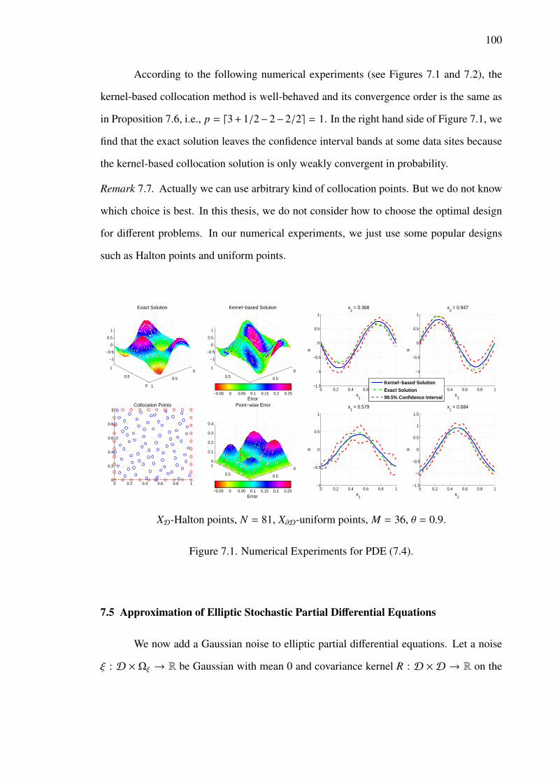
100
According to the following numerical experiments (see Figures 7.1 and 7.2), the
kernel-based collocation method is well-behaved and its convergence order is the same as
in Proposition 7.6, i.e., p = d3 + 1/2−2−2/2e = 1. In the right hand side of Figure 7.1, we
find that the exact solution leaves the confidence interval bands at some data sites because
the kernel-based collocation solution is only weakly convergent in probability.
Remark 7.7. Actually we can use arbitrary kind of collocation points. But we do not know
which choice is best. In this thesis, we do not consider how to choose the optimal design
for different problems. In our numerical experiments, we just use some popular designs
such as Halton points and uniform points.
0 0.2 0.4 0.6 0.8 10
0.2
0.4
0.6
0.8
1Collocation Points
0
0.5
10
0.5
1
−1
−0.5
0
0.5
1
Exact Solution
0
0.5
10
0.5
1
−1
−0.5
0
0.5
1
Kernel−based Solution
Error−0.05 0 0.05 0.1 0.15 0.2 0.25
0
0.5
10
0.5
1
0
0.1
0.2
0.3
0.4
Point−wise Error
Error−0.05 0 0.05 0.1 0.15 0.2 0.25
0 0.2 0.4 0.6 0.8 1−1.5
−1
−0.5
0
0.5
1
x1
ux
2 = 0.368
0 0.2 0.4 0.6 0.8 1−1.5
−1
−0.5
0
0.5
1
x1
u
x2 = 0.947
Kernel−based Solution
Exact Solution99.5% Confidence Interval
0 0.2 0.4 0.6 0.8 1−1
−0.5
0
0.5
1
x2
u
x1 = 0.579
0 0.2 0.4 0.6 0.8 1−1.5
−1
−0.5
0
0.5
1
1.5
x2
ux
1 = 0.684
XD-Halton points, N = 81, X∂D-uniform points, M = 36, θ = 0.9.
Figure 7.1. Numerical Experiments for PDE (7.4).
7.5 Approximation of Elliptic Stochastic Partial Differential Equations
We now add a Gaussian noise to elliptic partial differential equations. Let a noise
ξ : D × Ωξ → R be Gaussian with mean 0 and covariance kernel R : D × D → R on the

101
0.02 0.04 0.06 0.08 0.1 0.12 0.14 0.160.1
0.15
0.2
0.25
0.3
0.35
0.4
0.45
0.5
fill distance
real
tive
max
err
or
θ = 1.1
θ = 1.3
θ = 1.6
θ = 2.1
Figure 7.2. Convergence Rates for PDE (7.4).
probability space(Ωξ,Fξ,Pξ
). We use the Gaussian additive noise ξ to set up a stochastic
elliptic PDE, i.e., Pu = f + ξ, inD,
Bu = g, on ∂D,(7.5)
where f : D → R and g : ∂D → R. We select a positive definite kernel K : D ×D → R
such that the solution u of SPDE (7.5) almost surely belongs to its reproducing kernel
Hilbert space HK(D) which is embedded into the Sobolev space Hm(D) of order m >
n + d/2, where n := max O(P),O(B). Moreover, we suppose that its integral-type kernel∗
K satisfies the conditions (7.2).
Remark 7.8. In this section, we only discuss the noises on the right-hand side of SPDEs.
But we do not consider random coefficients on the left-hand side of SPDEs which we will
consider in our future work.
We firstly simulate the values of ξ at the collocation points XD, i.e.,
ξ :=(ξx1 , · · · , ξxN
)T∼ N
(0,AR,XD
),

102
where AR,XD :=(R(x j, xk)
)N,N
j,k=1. Consequently, the values at the collocation points XD and
X∂D
y j := f (x j) + ξx j , j = 1, · · · ,N, yN+ j := g(xN+ j), j = 1, · · · ,M,
are known and we denote that
yξ := (y1, · · · , yN , yN+1, · · · , yN+M)T .
Moreover, let pyξ ∼ N (mX,ΣX) be the probability density function of the multi normal
random vector yξ, where
mX := ( f (x1), · · · , f (xN), g(xN+1), · · · , g(xN+M))T , ΣX :=
AR,XD 0
0 0
∈ RN+M,N+M.
We define the product space(ΩKξ,FKξ,P
µξ
)with
ΩKξ := ΩK ×Ωξ, FKξ := FK ⊗ Fξ, Pµξ := Pµ ⊗ Pξ,
where the probability measure Pµ is defined on (HK(D),B (HK(D))) = (ΩK ,FK) as in
Theorem 7.2. We assume that the random variables defined on the original probability
spaces are extended to random variables on the new probability space in the natural way:
if random variables V1 : ΩK → R and V2 : Ωξ → R are defined on (ΩK ,FK ,Pµ) and(
Ωξ,Fξ,Pξ), respectively, then
V1(ω1, ω2) := V1(ω1), V2(ω1, ω2) := V2(ω2), for all ω1 ∈ ΩK and all ω2 ∈ Ωξ.
Note that in this case the random variables have the same probability distributional proper-
ties, and they are independent on(ΩKξ,FKξ,P
µξ
). This implies that the stochastic processes
PS , BS , S and ξ can be extended to the product space(ΩKξ,FKξ,P
µξ
)while preserving the
original probability distributional properties, and that (PS , BS , S ) and ξ are independent.
Moreover, since u can be seen as a map from Ωξ intoHK(D) = ΩK , we have u(·, ω2) ∈ ΩKξ
for all ω2 ∈ Ωξ.
103
We fix any x ∈ D. Let
Ex(v) :=ω1 × ω2 ∈ ΩKξ = ΩK ×Ωξ : ω1(x) = v
, v ∈ R,
and
EX(yξ(ω2)) :=ω1 × ω2 ∈ ΩKξ : Pω1(x1) = y1(ω2), . . . , Pω1(xN) = yN(ω2),
Bω1(xN+1) = yN+1(ω2), . . . , Bω1(xN+M) = yN+M(ω2) .
Since PS x(ω1, ω2) = PS x(ω1) = Pω1(x), BS x(ω1, ω2) = BS x(ω1) = Bω1(x), S x(ω1, ω2) =
S x(ω1) = ω1(x) and yξ(ω1, ω2) = yξ(ω2) for all ω1 ∈ ΩK and all ω2 ∈ Ωξ, we can approx-
imate the solution u(x, ω2) by the optimal estimator u(x, ω2) maximizing the conditional
probability given the data values yξ(ω2):
u(x, ω2) ≈ u(x, ω2) :=argmaxv∈R
supµ∈HK (D)
Pµξ
(Ex(v)
∣∣∣EX(yξ(ω2)))
=argmaxv∈R
supµ∈HK (D)
Pµξ
(S x = v
∣∣∣SX = yξ(ω2))
=argmaxv∈R
supµ∈HK (D)
pµx(v∣∣∣yξ(ω2)
)=∗
kX(x)T∗
KX−1yξ(ω2),
where the conditional probability density function pµx(·|·) is defined in Corollary 7.4. It is
obvious that u(·, ω2) ∈ HK(D) for all ω2 ∈ Ωξ.
Remark 7.9. If the collocation points X = XD ∪ X∂D are determined, then the random
part of u(x) is only related to yξ. We can formally rewrite u(x, ω2) as u(x, yξ) and u(x)
can be transferred to a random variable defined on the finite-dimensional probability space(RN+M,B
(RN+M
), µyξ
), where the probability measure µyξ is defined by µyξ(dv) := pyξ(v)dv.
Moreover, the probability distributional properties of u(x) do not change when(Ωξ,Fξ,Pξ
)is replaced by
(RN+M,B
(RN+M
), µyξ
).
Now we discuss the weak convergence of the kernel-based collocation solution. Let
Ex(ε) :=ω1 × ω2 ∈ ΩKξ : |ω1(x) − u(x, ω2)| ≥ ε
, ε > 0,

104
and
Ex(ε; X) :=ω1 × ω2 ∈ ΩKξ : |ω1(x) − u(x, ω2)| ≥ ε
and Pω1(x1) = y1(ω2), . . . , Pω1(xN) = yN(ω2),
Bω1(xN+1) = yN+1(ω2), . . . , Bω1(xN+M) = yN+M(ω2) .
We can deduce that
Pµξ (Ex(ε; X)) =
∫RN+MPµξ
(Ex(ε)
∣∣∣EX(v))µyξ(dv)
=
∫RN+MPµξ
(|S x − u(x, v)| ≥ ε
∣∣∣SX = v)µyξ(dv)
=
∫RN+M
∫|v−u(x,v)|≥ε
pµx(v|v)pyξ(v)dvdv
= erfc(
ε√
2σX(x)
),
where the variance σX(x)2 is defined in Corollary 7.4. According to Lemma 7.5, if P is an
elliptic differential operator of order 2 and B is an identity operator, then we have
supµ∈HK (D)
Pµξ (Ex(ε; X)) = O
hpX,D
ε
,where p := dm−2−d/2e and hX,D is the fill distance of X forD. Since |u(x, ω2) − u(x, ω2)| ≥
ε if and only if u(·, ω2) ∈ Ex(ε; X) we conclude that:
Proposition 7.7. If P is an elliptic differential operator of order 2 and B is an identity
operator, then
supµ∈HK (D)
Pµξ
(‖u − u‖L∞(D) ≥ ε
)≤ sup
µ∈HK (D),x∈DPµξ (Ex(ε; X))→ 0, when hX,D → 0,
for any ε > 0.
Therefore we say that the estimator u converges to the exact solution u in all proba-
bilities Pµξ when hX,D goes to 0. As in Section 7.4, ifHK(D) is dense inHm(D) with respect
to the Sobolev norm, then we can still say that u converges to u in probability even though
u ∈ Hm(D) almost surely.

105
7.5.1 Kernel-based Estimations for Regression. In this section, we construct another
kernel-based estimator using regression methods for smoothing spline models for obser-
vational data (see [24, 58]). For any given v ∈ RN+M, we can compute the conditional
expectation
m(x) :=∑v∈R
vP0ξ
(Ex(v)
∣∣∣EX(v))
=∑v∈R
vP0ξ
(S x = v
∣∣∣SX = v)
=EP0ξ
(S x
∣∣∣SX = v)
=∗
kX(x)T∗
KX−1v, x ∈ D.
So we can write m as a kernel-based regression model, i.e.,
m(x) =
N∑j=1
b jP2∗
K(x, x j) +
N+M∑j=N+1
b jB2∗
K(x, x j), x ∈ D,
where b1, . . . , bN+M ∈ R. Similar as in regression methods, y1, . . . , yN and yN+1, . . . , yN+M
can be thought of as the real-world observational data values of Pm(x1)+ξx1 , . . . , Pm(xN)+
ξxN and Bm(xN+1), . . . , Bm(xN+M) respectively. We use these observational data values to
compute the optimal coefficients of m from a ridge regression model, i.e.,
c := argminb∈RN+M
∥∥∥∥∥yξ −∗
KX b∥∥∥∥∥2
2+ bTΣX b =
(∗
KX + ΣX
)−1
yξ,
where ΣX ∈ R(N+M)×(N+M) is a covariance matrix of ξx1 , . . . , ξxN , 0, . . . , 0. Therefore, the
kernel-based estimation for regression has the form
u(x, ω2) ≈ u(x, ω2) = u(x, yξ(ω2)) =∗
kX(x)T(∗
KX + ΣX
)−1
yξ(ω2), x ∈ D.
According to Markov’s inequality [15] we have
ε2P0ξ (Ex(ε; X)) ≤ EP0
ξ
(EP0
ξ
(|S x − u(x)|2
∣∣∣SX = yξ))≤ σX(x)2, x ∈ D,
where ε > 0 and
σX(x)2 :=∗
K(x, x) −∗
kX(x)T(∗
KX + ΣX
)−1 (2ΣX + ΣX
∗
KX−1ΣX
) (∗
KX + ΣX
)−1 ∗kX(x).
7.5.2 Numerical Examples. Let the domain D := (0, 1)2 ⊂ R2 and the covariance kernel
of the Gaussian noise be
R(x, y) :=4π4 sin(πx1) sin(πx2) sin(πy1) sin(πy2)
+ 16π4 sin(2πx1) sin(2πx2) sin(2πy1) sin(2πy2).

106
We use the deterministic function
f (x) := −2π2 sin(πx1) sin(πx2) − 8π2 sin(2πx1) sin(2πx2)
and the Gaussian noise ξ with the covariance kernel R to set up the right hand side of the
stochastic Poisson equation with Dirichlet boundary condition, i.e.,∆u = f + ξ, inD,
u = 0, on ∂D.(7.6)
This means that P := ∆ and B := I|∂D and n = max O(P),O(B) = 2. Its exact solution has
the form
u(x) = sin(πx1) sin(πx2) + sin(2πx1) sin(2πx2) + ζ1 sin(πx1) sin(πx2)
+ζ2
2sin(2πx1) sin(2πx2), x = (x1, x2) ∈ D,
where ζ1, ζ2 are the independent standard normal random variable defined on(Ωξ,Fξ,Pξ
),
i.e., ζ1, ζ2 ∼ i.i.d. N(0, 1).
For the collocation methods, we use the Matern function G with shape parameter
θ > 0 and order m := 3 + 1/2 to set up the reproducing kernel K(x, y) := G(x − y) as in
Section 7.4.1. Next we choose Halton points inD and uniform grid points on ∂D as collo-
cation points. Using the kernel-based collocation method, we can set up the approximation
u defined as in Section 7.5.
We approximate the mean and variance of the arbitrary random variables U by its
sample mean and sample variance based on s := 10000 simulated sample paths using the
above algorithm, i.e.,
E(U) ≈1s
s∑k=1
U(ωk), Var(U) ≈1s
s∑k=1
U(ωk) −1s
s∑j=1
U(ω j)
2
.
According to the numerical results (see Figures 7.3 and 7.4), the approximate prob-
ability density functions are well-behaved. Its convergence order is also equal to p =
d3 + 1/2 − 2 − 2/2e = 1.

107
0
0.5
10
0.5
1
−0.5
0
0.5
1
1.5
Approximate Mean
Error0 0.05 0.1 0.15
0
0.5
10
0.5
1
0
0.5
1
Approximate Variance
Error−0.02 0 0.02 0.04 0.06 0.08 0.1
−4 −2 0 2 40
0.1
0.2
0.3
0.4
0.5
prob
abili
ty d
ensi
ty fu
nctio
n
x1 = 0.52632, x
2 = 0.52632
Empirical Theoretical
0 0.2 0.4 0.6 0.8 10
0.2
0.4
0.6
0.8
1Collocation Points
XD-Halton points, N = 81, X∂D-uniform points, M = 36, θ = 2.2.
Figure 7.3. Numerical Experiments for SPDE (7.6).
0.05 0.1 0.15 0.2 0.250
0.1
0.2
0.3
0.4
0.5
0.6
0.7
0.8
0.9
1
fill distance
rela
tive
max
err
or
Mean, θ = 1.6
Variance, θ = 1.6
Mean, θ = 2.6
Variance, θ = 2.6
Mean, θ = 3.6
Variance, θ = 3.6
Figure 7.4. Convergence Rates for SPDE (7.6).

108
7.6 Approximation of Parabolic Stochastic Partial Differential Equations
Suppose that(ΩW ,FW , Ft
Tt=0,PW
)is a stochastic basis with the usual assumptions.
We consider the following parabolic Ito equation
dUt = LUtdt + σdWt, inD, 0 < t < T,
BUt = 0, on ∂D,
U0 = u0,
(7.7)
where L is an elliptic differential operator of order 2, B is a boundary operator for Dirichlet
boundary conditions, u0 : D → R is a given deterministic function, and W is a Wiener
process with mean 0 and spatial covariance function R : D×D → R given by
E (Wt(x)Ws(y)) = mint, sR(x, y), x, y ∈ D, t, s > 0,
and the diffusion parameter σ > 0 (see for instance [9]).
We assume that SPDE (7.7) has a unique solution U ∈ L2 (ΩW × (0,T );Hm(D)),
where m > 2 + d/2.
The proposed numerical method for solving a general SPDE of the form (7.7) can
be described as follows:
1.) Discretize SPDE (7.7) in time by the implicit Euler scheme at equally spaced time
points 0 = t0 < t1 < . . . < tn = T ,
Uti − Uti−1 = LUtiδt + σδWi, i = 1, . . . , n, (7.8)
where δt := ti − ti−1 = T/n and δWi := Wti −Wti−1 .
2.) Under the assumption that the noise at each time step ti is independent from the
solution Uti−1 at the previous step, we simulate the Gaussian field with covariance
structure R(x, y) at a finite collection of predetermined collocation points
XD := x1, · · · , xN ⊂ D, X∂D := xN+1, · · · , xN+M ⊂ ∂D.

109
3.) Let the differential operator P := I − δtL, and the noise term ξ := σδWi. It is easy
to check that P is the elliptic differential operator of order 2 and ξ is a Gaussian
field with mean E (ξx) = 0 and covariance kernel Cov(ξx, ξy
)= σ2δtR(x, y). Equa-
tion (7.8) together with the corresponding boundary condition becomes an elliptic
SPDE of the form Pu = f + ξ, inD,
Bu = 0, on ∂D,(7.9)
where u := Ut j is seen as an unknown part and f := Uti−1 and ξ are viewed as given
parts. We solve for u using the kernel-based collocation method as in Section 7.5,
i.e.,
u(x) ≈ u(x) :=N∑
k=1
ckP2∗
K(x, xk) +
M∑k=1
cN+kB2∗
K(x, xN+k),
where the reproducing kernel Hilbert space HK(D) of the reproducing kernel K :
D×D → R is equivalent to the Sobolev spaceHm(D) and its integral-type kernel∗
K
satisfies the conditions (7.2). The unknown random coefficients c := (c1, · · · , cN+M)T
are obtained by solving a random system of linear equations, i.e.,
∗
KX c = yξ,
where the interpolation matrix∗
KX is set up as in Corollary 7.3 and the random vector
yξ := (y1, · · · , yN , yN+1, · · · , yN+M)T is given by
y j := f (x j) + ξx j , j = 1, · · · ,N, yN+ j := 0, j = 1, · · · ,M.
Here f (x1), . . . , f (xN) can be computed at the previous time step ti−1 and ξxN+1 , . . . , ξxN+M
can be simulated by a multi-normal vector. When i − 1 = 0, then f (x j) = u0(x j) for
all j = 1, . . . ,N.
4.) Repeat S2 and S3 for all i = 1, . . . , n.
Using our kernel-based collocation method we can perform the computations to
numerically estimate the sample paths uij ≈ Uti(x j). An algorithm to solve SPDE (7.8) is

110
1. Initialize
• u0 := (u0(x1), · · · , u0(xN))T
•∗
KX :=
(P1P2
∗
K(x j, xk))N,N
j,k=1,
(P1B2
∗
K(x j, xN+k))N,M
j,k=1(B1P2
∗
K(xN+ j, xk))M,N
j,k=1,
(B1B2
∗
K(xN+ j, xN+k))M,M
j,k=1
• BX :=
(P2∗
K(x j, xk))N,N
j,k=1,
(B2∗
K(x j, xN+k))N,M
j,k=1
• Σξ := σ2δt
(R(x j, xk)
)N,N
j,k=1, δt := T/n
• AX := BX
∗
KX−1
2. Repeat for i = 1, 2, . . . , n, i.e., for t1, t2, . . . , tn = T
• Simulate ξ ∼ N(0,Σξ
)• ui := BX
∗
KX−1
ui−1 + ξ
0
= AX
ui−1 + ξ
0
Note that in the very last step the matrix AX is pre-computed and can be used for all time
steps, and for different sample paths; that makes the proposed algorithm to be quite effi-
cient.
Now we discuss the error bound of this algorithm. Let U i be the exact solution
of the elliptic SPDE (7.9) for each time step ti. Similar as the Euler method of SODE
(see [33]), we can use the Ito formula
Uti − Uti−1 =
∫ ti
ti−1
LUtdt + σ
∫ ti
ti−1
dWt.
to deduce that
Uti − U i D= O
(δt1/2
).
Here D= means to be equal in distribution. Denote that the numerical error at the collocation
points XD at time step ti is given by
ei := Uti − ui,
111
where Uti :=(Uti(x1), · · · ,Uti(xN)
)T . Combining the convergence orders of the kernel-
based collocation method discussed in Section 7.5, we have
ei D= AXei−1 + O
(hp
X,D
)+ O
((δt1/2
)),
where p := dm − 2 − d/2e. By induction, we can deduce that
en D=
(I + AX + · · · + An−1
X
) (O
(hp
X,D
)+ O
(δt1/2
)).
Suppose that the spectral radius r := ρ(AX) of AX satisfies r < 1. Thus
1√
N‖en‖2
D=
1 − rn
1 − r
(O
(hp
X,D
)+ O
(δt1/2
)).
Moreover [25] shows that the spectral radius r ∼ δt/h2X,D for the Sobolev-spline kernels with
the well-behaved shape parameters. This implies that ui is convergent to Uti in distribution
when both δt and hX,D go to zero.
Remark 7.10. We should mention that even for deterministic time-dependent PDEs to find
the exact rates of convergence of kernel-based methods is a delicate and nontrivial question,
only recently solved in [25]. We will address this question in the case of SPDEs in future
works.
7.6.1 Stochastic Parabolic Equations with Multiplicative Noise. In addition to the ad-
ditive noise case discussed here, we can also use the kernel-based collocation method to
approximate other well-posed stochastic parabolic equations with multiplicative noise, e.g.,
dUt = LUtdt + Σ (Ut) dWt, inD, 0 < t < T,
BUt = 0, on ∂D,
U0 = u0,
(7.10)
where Σ ∈ C2(R). Since∫ ti
ti−1Σ (Ut) dWt ≈ Σ
(Uti−1
)δWi, the algorithm for SPDE (7.10) is
similar to before:

112
1. Initialize
• u0 := (u0(x1), · · · , u0(xN))T
•∗
KX :=
(P1P2
∗
K(x j, xk))N,N
j,k=1,
(P1B2
∗
K(x j, xN+k))N,M
j,k=1(B1P2
∗
K(xN+ j, xk))M,N
j,k=1,
(B1B2
∗
K(xN+ j, xN+k))M,M
j,k=1
• BX :=
(P2∗
K(x j, xk))N,N
j,k=1,
(B2∗
K(x j, xN+k))N,M
j,k=1
• ΣR := δt
(R(x j, xk)
)N,N
j,k=1, δt := T/n
• AX := BX
∗
KX−1
2. Repeat for i = 1, 2, · · · , n, i.e., for t1, t2, · · · , tn = T
• V := diag(Σ(ui−1
1
), · · · ,Σ
(ui−1
N
))• Σξ := VTΣRV
• Simulate ξ ∼ N(0,Σξ
)
• ui := BX
∗
KX−1
ui−1 + ξ
0
= AX
ui−1 + ξ
0
7.6.2 Numerical Examples. We consider the stochastic heat equation with Dirichlet
boundary conditions
dUt = d2
dx2 Utdt + σdWt,i, inD := (0, 1) ⊂ R, 0 < t < T := 1,
Ut = 0, on ∂D,
U0 = u0,
(7.11)
driven by two types of space-time white noise (colored in space) W of the form
Wt,i :=∞∑
k=1
W (k)t qi
kψk, qk :=1kπ, ψk(x) :=
√2 sin(kπx),

113
where W (k)t , k ∈ N, is a sequence of independent scalar Brownian motions, and i = 1, 2
(see Appendix A). Note that choosing the larger value of i corresponds to a noise that is
smoother in space. Here the diffusion parameter σ > 0 and the initial condition is given by
u0(x) :=√
2 (sin(πx) + sin(2πx) + sin(3πx)) , x ∈ D.
The spatial covariance function Ri(x, y) =∑∞
k=1 q2ik ψk(x)ψk(y), i = 1, 2, takes the
specific forms
R1(x, y) = minx, y − xy, 0 < x, y < 1,
and
R2(x, y) =
−1
6 x3 + 16 x3y + 1
6 xy3 − 12 xy2 + 1
3 xy, 0 < x < y < 1,
−16y3 + 1
6 xy3 + 16 x3y − 1
2 x2y + 13 xy, 0 < y < x < 1.
The solution of SPDE (7.11) is given by (for more details see, for instance, [9])
Ut(x) =
∞∑k=1
ξt,kψk(x), x ∈ D, 0 < t < T,
where
ξ0,k :=∫ 1
0u0(x)ψk(x)dx, ξt,k := ξ0,ke−k2π2t +
σ
qik
∫ t
0ek2π2(s−t)dWk
s .
From this explicit solution we can get that
E (Ut(x)) =
∞∑k=1
ξ0,ke−k2π2tψk(x), Var (Ut(x)) =
∞∑k=1
σ2
2k2π2q2ik
(1 − e−2k2π2t) |ψk(x)|2 .
We discretize the time interval [0,T ] with n equal time steps so that δt := T/n. We
also choose the reproducing kernel K(x, y) := G(x − y), where
G(x) :=(3 + 3θ |x| + θ2 |x|2
)e−θ|x|, x ∈ R,
is the Matern function with shape parameter θ > 0 and order m := 3 as in Example 4.4. So
its integral-type kernel∗
K has the form∗
K(x, y) =
(632θ
+632|x − y| + 14θ |x − y|2 +
7θ2
2|x − y|3 +
θ3
2|x − y|4
+θ4
30|x − y|5
)e−θ|x−y| + H(x, y), x, y ∈ D.

114
where
H(x, y) :=(−
634θ−
454
(x + y) −17θ2
xy −5θ2
(x2 + y2
)− 2θ2
(xy2 + x2y
)−θ3
2x2y2
)e−θ(x+y)
+
(−θ3
2− 4θ2 −
27θ2−
452−
634θ
+
(θ3 + 6θ2 +
27θ2
+454
)(x + y)
+
(−2θ3 − 8θ2 −
17θ2
)xy +
(−θ3
2− 2θ2 −
5θ2
) (x2 + y2
)+
(θ3 + 2θ2
) (xy2 + x2y
)−θ3
2x2y2
)eθ(x+y−2).
As collocation points we select uniform grid points XD ⊂ (0, 1) and X∂D := 0, 1. Let
P := I−δtd2/dx2 and B := I|0,1. We also have p = d3−2−1/2e = 1. Using our kernel-based
collocation method we can perform the following computations to numerically estimate the
sample paths uij ≈ Uti(x j).
We approximate the mean and variance of Ut(x) by sample mean and sample vari-
ance from s := 10000 simulated sample paths using the above algorithm, i.e.,
E(Uti(x j)
)≈
1s
s∑k=1
uij(ωk), Var
(Uti(x j)
)≈
1s
s∑l=1
uij(ωl) −
1s
s∑k=1
uij(ωk)
2
.
Figure 7.5 shows that the histograms at different values of t and x resemble the
theoretical normal distributions. Our use of an implicit time stepping scheme reduces the
frequency of the white noise, i.e., limδt→0 δW/δt ∼ δ0. Consequently, Figure 7.6 shows
that the approximate mean is well-behaved but the approximate variance is a little smaller
than the exact variance. According to Figure 7.7 we find that this numerical method is
convergent as both δt and hX,D are refined. Finally, we want to mention that the distribution
of collocation points, the shape parameter, and the kernel itself were chosen empirically
and based on the authors’ experience. The convergence rate is close to our discussion in
Section 7.6, i.e., relative error ∼ O(hX,D + δt1/2
).
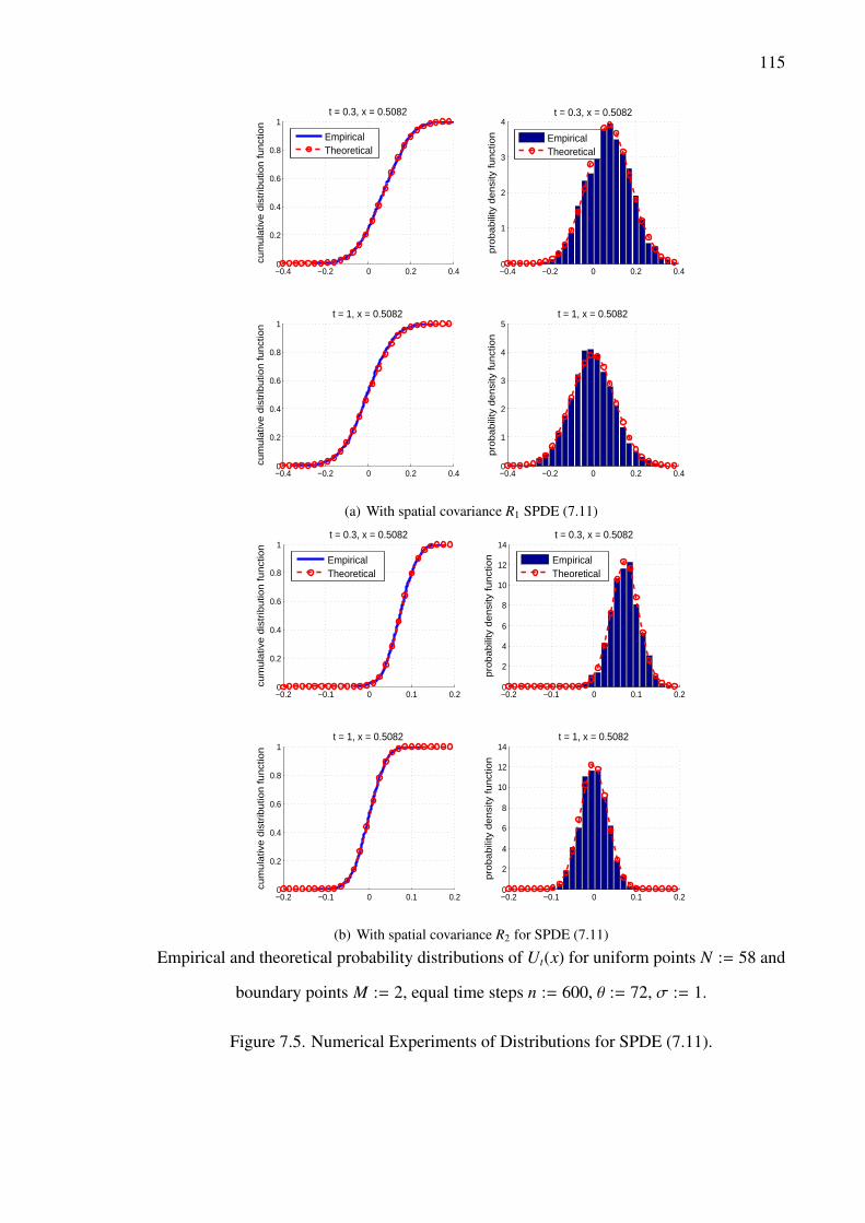
115
−0.4 −0.2 0 0.2 0.40
0.2
0.4
0.6
0.8
1
cum
ula
tive
dis
trib
utio
n f
un
ctio
n
t = 0.3, x = 0.5082
EmpiricalTheoretical
−0.4 −0.2 0 0.2 0.40
1
2
3
4
pro
ba
bili
ty d
en
sity
fu
nct
ion
t = 0.3, x = 0.5082
EmpiricalTheoretical
−0.4 −0.2 0 0.2 0.40
0.2
0.4
0.6
0.8
1
cum
ula
tive
dis
trib
utio
n f
un
ctio
n
t = 1, x = 0.5082
−0.4 −0.2 0 0.2 0.40
1
2
3
4
5
pro
ba
bili
ty d
en
sity
fu
nct
ion
t = 1, x = 0.5082
(a) With spatial covariance R1 SPDE (7.11)
−0.2 −0.1 0 0.1 0.20
0.2
0.4
0.6
0.8
1
cum
ula
tive
dis
trib
utio
n f
un
ctio
n
t = 0.3, x = 0.5082
EmpiricalTheoretical
−0.2 −0.1 0 0.1 0.20
2
4
6
8
10
12
14
pro
ba
bili
ty d
en
sity
fu
nct
ion
t = 0.3, x = 0.5082
EmpiricalTheoretical
−0.2 −0.1 0 0.1 0.20
0.2
0.4
0.6
0.8
1
cum
ula
tive
dis
trib
utio
n f
un
ctio
n
t = 1, x = 0.5082
−0.2 −0.1 0 0.1 0.20
2
4
6
8
10
12
14
pro
ba
bili
ty d
en
sity
fu
nct
ion
t = 1, x = 0.5082
(b) With spatial covariance R2 for SPDE (7.11)
Empirical and theoretical probability distributions of Ut(x) for uniform points N := 58 and
boundary points M := 2, equal time steps n := 600, θ := 72, σ := 1.
Figure 7.5. Numerical Experiments of Distributions for SPDE (7.11).

116
(a) With spatial covariance R1 for SPDE (7.11)
(b) With spatial covariance R2 for SPDE (7.11)
Approximate and theoretical means and variances for uniform points N := 58 and M := 2,
equal time steps n := 600, θ := 72, σ := 1.
Figure 7.6. Numerical Experiments of Mean and Variance for SPDE (7.11).

117
1 1.5 2 2.5
x 10−3
0.1
0.15
0.2
0.25
0.3
0.35
0.4
0.45
δ t
rela
tive
root
mea
n sq
uare
err
or
Mean, fill distance=3.03e−002
Variance, fill distance=3.03e−002
Mean, fill distance=2.00e−002
Variance, fill distance=2.00e−002
Mean, fill distance=1.00e−002
Variance, fill distance=1.00e−002
(a) With spatial covariance R1 for SPDE (7.11)
1 1.5 2 2.5
x 10−3
0.08
0.1
0.12
0.14
0.16
0.18
0.2
0.22
0.24
0.26
δ t
rela
tive
root
mea
n sq
uare
err
or
Mean, fill distance=3.03e−002
Variance, fill distance=3.03e−002
Mean, fill distance=2.00e−002
Variance, fill distance=2.00e−002
Mean, fill distance=1.00e−002
Variance, fill distance=1.00e−002
(b) With spatial covariance R2 for SPDE (7.11)
Convergence of mean and variance with respect to refinement of collocation points and
time steps for σ := 1, and the relative RMSE of exact u and approximate u is defined by
error(u, u) :=√
1n
n∑i=1
‖ui−ui‖22
‖ui‖22
where ui, ui ∈ RN are the numerical values at the collocation points for each time step ti.
Figure 7.7. Convergence Rates for SPDE (7.11).

118
CHAPTER 8
FUTURE WORK
Even though we have presented the unified theories for the relationships of repro-
ducing kernels and Green functions in this thesis, there are still a lot of unknown fields we
need to discuss more deeply.
8.1 Pseudo-differential Operators
The vector distributional operator P can be constructed by pseudo-differential op-
erators. Therefore their generalized Sobolev spaces HP(Rd) are isometrically equivalent
to the Beppo-Levi type spaces Xmτ (Rd). The paper [7] shows that the radial basis function
under tension may be associated to a pseudo-differential operator in a Beppo-Levi space.
For example, if
P :=
ωτF∂m
∂xm1, · · · ,
√m!α!ωτFDα, · · · , ωτF
∂m
∂xmd
T
,
then
HP(Rd) ≡ Xmτ (Rd) :=
f ∈ Lloc
1 (Rd) ∩ SI : ωτDα f ∈ L2(Rd) for all α ∈ Nd0 with |α| = m
,
where F is a distributional Fourier transform map and ωτ(x) := ‖x‖τ2, 0 6 τ < 1. However,
P may not satisfy the condition of Theorem 4.2. We have reserved these situations for our
future research.
8.2 Singular Green Kernels
We now present a standard singular Green kernel example from the theory of partial
differential equations (see [17, Chapter 2.2]) similar as our construction in Section 5.3. In
order to solve Poisson’s equation in the d-dimensional (d ≥ 2) open unit ballD := B(0, 1) =x ∈ Rd : ‖x‖2 < 1
with (homogeneous) Dirichlet boundary condition, one constructs the
non-symmetric Green kernel
G(x, y) := Φ(x − y) − Φ(‖x‖2 y − x), x, y ∈ D,
119
of the Laplace operator L := −∆ = −∑d
j=1∂2
∂x2j
subject to the given boundary condition,
where Φ is the fundamental solution of −∆ given by
Φ(x) :=
− 1
2π log ‖x‖2 , d = 2,
Γ(d/2+1)d(d−2)πd/2 ‖x‖2−d
2 , d ≥ 3.
Just as in our discussion below, the Laplace operator L = −∆ = P∗T P = −∇T∇ can be
computed using the gradient P := (P1, · · · , Pd)T = ∇ =(∂∂x1, · · · , ∂
∂xd
)Tand its distributional
adjoint operator P∗ :=(P∗1, · · · , P
∗d
)T= −∇. With the help of Green’s formulas [17] we can
further check that the kernel G has a reproduction property with respect to the gradient-
inner product on C10(D), i.e., for all f ∈ C1
0(D) ⊂ H0P(D) H1
0 (D) and all y ∈ D, we
have
( f ,G(·, y))P,D =
d∑j=1
(P j f , P jG(·, y)
)D
=
d∑j=1
∫D
∂ f (x)∂x j
∂G(x, y)∂x j
dx = f (y).
But this Green kernel G is not a reproducing kernel as in Definition 2.1 because G is sin-
gular along its diagonal, i.e., G(x, x) = ∞ for all x ∈ D. Schaback said that the singular
kernel might be able to use for interpolation problems. In our future work we want to
change the definition of the reproducing kernel such that the singular kernel is still a gen-
eralized reproducing kernel which can be used for scattered data approximation.
8.3 Optimal Shape Parameters
According to this thesis, we can construct various kinds of reproducing kernels.
However, it is still an open problem how to find the “optimal” kernel to approximate a
given target function. One of my future research topics is to find the optimal shape param-
eter of the kernel function. Example 4.4 shows that the reproducing kernel Hilbert spaces
induced by Matern functions can be seen to redefine the classical L2-based Sobolev spaces
employing different inner products in terms of shape parameters. This indicates that the
shape parameter will control the reproducing norm by affecting the weight of the various
derivatives involved. This may guide us in finding the kernel function with optimal shape

120
parameter to set up a kernel-based approximation for a given set of data values–an impor-
tant problem in practice for which no analytical solution exists.
8.4 Kernel-based Collocation Methods for SPDEs
The kernel-based collocation method can also be used to approximate systems of
elliptic SPDEs derived by vector Gaussian noises ξ1 and ξ2 or nonlinear SPDEs derived by
a Gaussian noise ξ, i.e.,Pu = f + ξ1, inD,
Bu = g + ξ2, on ∂D,or
F(Pu) = Σ( f , ξ), inD,
G(Bu) = g, on ∂D,
where P :=(P1, · · · , Pnp
)Tand B :=
(B1, · · · , Bnb
)T are a vector differential operator and
a vector boundary operator, respectively, and F ∈ C2(Rnp), G ∈ C2(Rnb), and Σ ∈ C2(R2).
We only discuss the rates of convergence of seconde-order elliptic differential equations in
Lemma 7.5. But we can also introduce the error bounds of the high-order elliptic differen-
tial equations with well-behaved boundary conditions in the similar way, i.e.,
|σX(x)| ≤np∑j=1
CP, j
∥∥∥∥∥PP j,1P j,2
∗
K,XD
∥∥∥∥∥L∞(D)
+
nb∑j=1
CB, j
∥∥∥∥∥PB j,1B j,2
∗
K,X∂D
∥∥∥∥∥L∞(∂D)
= O(hp1
XD,D
)+O
(hp2
X∂D,∂D
),
where CP, j,CB, j are positive constants independent on x ∈ D, and p1 := dm − O(P) −
d/2e, p2 := dm−O(B)− d/2e (here the integral-type kernel∗
K defined in Theorem 7.2). As
mentioned before, more precise methods for parabolic SPDEs are currently not available.
We will try to find the connections of reproducing kernels and noise covariance kernels
to choose the “best” reproducing kernel for different SPDE problems by the kernel-based
collocation methods. A rigorous investigation of these questions, as well as determination
of precise rates of convergence is reserved for our future work.

121
APPENDIX A
WHITE NOISE AND STOCHASTIC PARTIAL DIFFERENTIAL EQUATIONS
122
Definition A.1 ([31, Definition A] and [45, Definition 2.2.1]). A scalar Brownian motion
(Wiener process) is a continuous process adapted process Wt defined on some probability
space(Ω,F , Ft
∞t=0 ,P
), with the properties that W0 = 0 a.s. and for 0 ≤ s < t, the increment
Wt −Ws is independent of Fs and its normally distributed with mean 0 and variance t − s.
Theorem A.1 ([45, Theorem 5.2.1] (existence and uniqueness theorem for stochastic ordi-
nary differential equations)). Let Wt be a scalar Brownian motion defined on some proba-
bility space(Ω,F , Ft
∞t=0 ,P
). Suppose that the drift b : [0,T ] × R → R and the diffusion
Σ : [0,T ] × R→ R are measurable functions satisfying
|b(t, x)| + |Σ(t, x)| ≤ C1 (1 + |x|) , x ∈ R, t ∈ [0,T ],
and
|b(t, x) − b(t, y)| + |Σ(t, x) − Σ(t, y)| ≤ C2 |x − y| , x ∈ R, t ∈ [0,T ],
for some positive constants C1 and C2. Then the stochastic ordinary differential equationdXt = b(t, Xt)dt + Σ(t, Xt)dWt, 0 < t < T,
X0 = x ∈ R,
has a unique t-continuous solution and X ∈ L2 (Ω × (0,T )).
Definition A.2 ([9, Section 3.2]). Suppose that R is a semi-positive definite kernel defined
on a domain D ⊂ Rd andW (k)
t
∞k=1
is a sequence of independent, identically distributed
standard scalar Brownian motions defined on some probability space(Ω,F , Ft
∞t=0 ,P
). If
qk∞k=1 are the eigenvalues of R and their related normalized eigenfunctions ψk
∞k=1 are
some complete orthonormal bases of a Hilbert spaceH composing of functions defined on
D, then
Wt :=∞∑
k=1
W (k)t√
qkψk
is called a Wiener process in the Hilbert spaceH with spatial covariance operator R defined
on the probability space(Ω,F , Ft
∞t=0 ,P
).
123
Theorem A.2 ([9, Theorem 6.3 in Section 3.3]). Let Wt be a Wiener process in the Hilbert
spaceH with spatial covariance operator R defined on some probability space(Ω,F , Ft
∞t=0 ,P
).
Suppose that the drift b : [0,T ] × H → L2(D) and the diffusion Σ : [0,T ] × H → L2(D)
are measurable functions satisfying
‖b(t, f )‖L2(D) + ‖Σ(t, f )‖L2(D) ≤ C1(1 + ‖ f ‖H
), f ∈ H , t ∈ [0,T ],
and
‖b(t, f ) − b(t, g)‖L2(D) + ‖Σ(t, f ) − Σ(t, g)‖L2(D) ≤ C2 ‖ f − g‖H , f , g ∈ H , t ∈ [0,T ],
for some positive constants C1 and C2. Then the stochastic partial differential equation
dUt = (κ∆ − θI) Ut + b(t,Ut) + Σ(t,Ut)dWt, inD, 0 < t < T,
BUt = 0, on ∂D,
U0 = u0 ∈ H ,
has a unique (mild) solution Ut which is a continuous adapted process in H and U ∈
L2 (Ω × (0,T );H), where κ, θ ≥ 0 and B is a boundary operator for Dirichlet or Neumann
boundary conditions.

124
BIBLIOGRAPHY
[1] Mathematics Genealogy Project. http://www.genealogy.ams.org/.
[2] R. A. Adams and J. J. F. Fournier. Sobolev Spaces, volume 140 of Pure and AppliedMathematics (Amsterdam). Elsevier/Academic Press, Amsterdam, 2003.
[3] E. Alpaydin. Introduction to Machine Learning. MIT Press, 2010.
[4] I. Babuska, F. Nobile, and R. Tempone. A stochastic collocation method for ellipticpartial differential equations with random input data. SIAM Rev., 52(2):317–355,2010.
[5] A. Berlinet and C. Thomas-Agnan. Reproducing Kernel Hilbert Spaces in Probabilityand Statistics. Kluwer Academic Publishers, 2004.
[6] S. Bochner. Vorlesungen uber Fouriersche Integrale, volume 12 of Mathematik undihre Anwendungen. Akad. Verlagsges., Leipzig, 1932.
[7] A. Bouhamidi. Pseudo-differential operator associated to the radial basis functionsunder tension. In RFMAO 05—Rencontres Franco-Marocaines en Approximation etOptimisation 2005, volume 20 of ESAIM Proc., pages 72–82. EDP Sci., Les Ulis,2007.
[8] M. D. Buhmann. Radial Basis Functions: Theory and Implementations, volume 12of Cambridge Monographs on Applied and Computational Mathematics. CambridgeUniversity Press, 2003.
[9] P-L. Chow. Stochastic Partial Differential Equations. Chapman & Hall/CRC AppliedMathematics and Nonlinear Science Series. Chapman & Hall/CRC, Boca Raton, FL,2007.
[10] I. Cialenco, G. E. Fasshauer, and Q. Ye. Approximation of stochastic partial differ-ential equations by a kernel-based collocation method. Int. J. Comput. Math., 2012.Special Issue: Recent Advances on the Numerical Solutions of Stochastic Partial Dif-ferential Equations, DOI: 10.1007/s10444-011-9264-6.
[11] R. J. P. de Figueiredo and G. R. Chen. PDLg splines defined by partial differential op-erators with initial and boundary value conditions. SIAM J. Numer. Anal., 27(2):519–528, 1990.
[12] M. K. Deb, I. M. Babuska, and J. T. Oden. Solution of stochastic partial differentialequations using Galerkin finite element techniques. Comput. Methods Appl. Mech.Engrg., 190(48):6359–6372, 2001.
[13] P. Diaconis. Bayesian numerical analysis. in Statistical Decision Theory and RelatedTopics IV, Papers from the 4th Purdue Symp., West Lafayette/Indiana 1986. S. S. Guptaand J. O. Berger (eds.), Vol. 1. Springer-Verlag, pages 163–175, 1988.
[14] J. Duchon. Splines minimizing rotation-invariant semi-norms in sobolev spaces. In:Schempp, W and Zeller, K (eds.) Constructive Theory of Functions of Several Vari-ables, Springer Berlin, pages 85–100, 1977.
[15] R. Durrett. Probability: Theory and Examples. Duxbury Press, 1996.
125
[16] J. F. Erickson. Generalized Native Spaces. Doctor of philosophy in applied mathe-matics, Illinois INstitute of Technology, Chicago, Illinois, 2007.
[17] L. C. Evans. Partial Differential Equations, volume 19 of Graduate Studies in Math-ematics. American Mathematical Society, second edition, 2010.
[18] G. E. Fasshauer. Meshfree Approximation Methods with Matlab, volume 6 of In-terdisciplinary Mathematical Sciences. World Scientific Publishing Co. Pte. Ltd.,Hackensack, NJ, 2007.
[19] G. E. Fasshauer. Positive definite kernels: past, present and future. Dolomite ResearchNotes on Approximation, 4:21–63, 2011.
[20] G. E. Fasshauer and Q. Ye. Reproducing kernels of generalized Sobolev spaces viaa Green function approach with distributional operators. Numer. Math., 119(3):585–611, 2011.
[21] G. E. Fasshauer and Q. Ye. Reproducing kernels of Sobolev spaces via a Green kernelapproach with differential operators and boundary operators. Adv. Comput. Math.,2011. DOI: 10.1007/s10444-011-9264-6.
[22] G. E. Fasshauer and Q. Ye. Kernel-based collocation methods versus Galerkin finiteelement methods for approximating elliptic stochastic partial differential equations.Meshfree Methods for Partial Differential Equations VI, Springer series: LectureNotes in Computational Science and Engineering, 2012. to appear.
[23] C. F. Gauß. Theory of The Motion of The Heavenly Bodies Moving about The Sun inConic Sections. Hamburg: Friedrich Perthes and I. H. Besser, 1809.
[24] T. Hastie, R. Tibshirani, and J. Friedman. The Elements of Statistical Learning.Springer Series in Statistics. Springer, second edition, 2009. Data mining, inference,and prediction.
[25] Y. C. Hon and R. Schaback. The kernel-based method of lines for the heat equation.2010. University of Gottingen, preprint.
[26] L. Hormander. The Analysis of Linear Partial Differential Operators. I. Classics inMathematics. Springer-Verlag, 2003.
[27] J. K. Hunter and B. Nachtergaele. Applied Analysis. World Scientific Publishing Co.Inc., 2001.
[28] A. Iske. Multiresolution methods in scattered data modelling, volume 37 of LectureNotes in Computational Science and Engineering. Springer-Verlag, 2004.
[29] S. Janson. Gaussian Hilbert Spaces, volume 129 of Cambridge Tracts in Mathemat-ics. Cambridge University Press, 1997.
[30] A. Jentzen and P. E. Kloeden. Recent Advances in the Numerical Approximationof Stochastic Partial Differential Equations – Taylor Approximations of StochasticPartial Differential Equations. CBMS Lecture. 2010.
[31] I. Karatzas and S. E. Shreve. Brownian Motion and Stochastic Calculus, volume 113of Graduate Texts in Mathematics. Springer-Verlag, 1991.
[32] A. Khintchine. Korrelationstheorie der stationaren stochastischen Prozesse. Math.Ann., 109(1):604–615, 1934.

126
[33] P. E. Kloeden and E. Platen. Numerical Solution of Stochastic Differential Equations,volume 23 of Applications of Mathematics (New York). Springer-Verlag, 1992.
[34] J. Kybic, T. Blu, and M. Unser. Generalized sampling: a variational approach. I, II.Theory. IEEE Trans. Signal Process., 50(8):1965–1985, 2002.
[35] W. Light and H. Wayne. Spaces of distributions, interpolation by translates of a basisfunction and error estimates. Numer. Math., 81(3):415–450, 1999.
[36] M. N. Lukic and J. H. Beder. Stochastic processes with sample paths in reproducingkernel Hilbert spaces. Trans. Amer. Math. Soc., 353(10):3945–3969, 2001.
[37] W. R. Madych and S. A. Nelson. Multivariate interpolation and conditionally positivedefinite functions. II. Math. Comp., 54(189):211–230, 1990.
[38] M. Mathias. Uber positive Fourier-Integrale. Math. Z., 16(1):103–125, 1923.
[39] R. E. Megginson. An Introduction to Banach Space Theory. Graduate texts in math-ematics. Springer-Verlag, 1998.
[40] J. Mercer. Functions of positive an negative type and their connection with the theoryof integral equations. Philosophical Transactions of the Royal Society of London.Series A, Containing Papers of a Mathematical or Physical Character, 209:415–446,1909.
[41] C. A. Micchelli. Interpolation of scattered data: distance matrices and conditionallypositive definite functions. In Approximation theory and spline functions (St. John’s,Nfld., 1983), volume 136 of NATO Adv. Sci. Inst. Ser. C Math. Phys. Sci., pages 143–145. Reidel, Dordrecht, 1984.
[42] C. A. Micchelli. Interpolation of scattered data: distance matrices and conditionallypositive definite functions. Constr. Approx., 2(1):11–22, 1986.
[43] F. Nobile, R. Tempone, and C. G. Webster. An anisotropic sparse grid stochasticcollocation method for partial differential equations with random input data. SIAM J.Numer. Anal., 46(5):2411–2442, 2008.
[44] F. Nobile, R. Tempone, and C. G. Webster. A sparse grid stochastic collocationmethod for partial differential equations with random input data. SIAM J. Numer.Anal., 46(5):2309–2345, 2008.
[45] B. Øksendal. Stochastic Differential Equations. Universitext. Springer-Verlag, 2003.
[46] W. Rudin. Real and Complex Analysis, 3rd ed. McGraw-Hill, Inc., 1987.
[47] R. Schaback. Creating surfaces from scattered data using radial basis functions. pages477–496, 1995.
[48] R. Schaback. Spectrally optimized derivative formulae. 2008. In: Data Page of R.Schaback’s Research Group.
[49] R. Schaback and H. Wendland. Kernel techniques: from machine learning to meshlessmethods. Acta Numer., 15:543–639, 2006.
[50] M. Scheuerer, R. Schaback, and M. Schlather. Interpolation of spatial data – a stochas-tic or a deterministic problem? 2010. University of Gottingen, preprint.

127
[51] I. J. Schoenberg. Metric spaces and completely monotone functions. Ann. of Math.(2), 39(4):811–841, 1938.
[52] G. Song, J. Riddle, E. G. Fasshauer, and F. Hickernell. Multivariate interpolationwith increasingly flat radial basis functions of finite smoothness. Adv. Comput. Math.,36(3):485–501, 2012.
[53] E. M. Stein and G. Weiss. Introduction to Fourier analysis on Euclidean spaces.Princeton University Press, 1971.
[54] M. L. Stein. Interpolation of Spatial Data. Springer Series in Statistics. Springer-Verlag, 1999. Some theory for Kriging.
[55] I. Steinwart and A. Christmann. Support Vector Machines. Springer, 2008.
[56] J. Stewart. Positive definite functions and generalizations, an historical survey. RockyMountain J. Math., 6(3):409–434, 1976.
[57] G. Wahba. Bayesian “confidence intervals” for the cross-validated smoothing spline.J. Roy. Statist. Soc. Ser. B, 45(1):133–150, 1983.
[58] G. Wahba. Spline Models for Observational Data, volume 59 of CBMS-NSF Re-gional Conference Series in Applied Mathematics. Society for Industrial and AppliedMathematics (SIAM), 1990.
[59] H. Wendland. Piecewise polynomial, positive definite and compactly supported radialfunctions of minimal degree. Adv. Comput. Math., 4(4):389–396, 1995.
[60] H. Wendland. Scattered Data Approximation, volume 17 of Cambridge Monographson Applied and Computational Mathematics. Cambridge University Press, 2005.
[61] Q. Ye. Reproducing kernels of generalized Sobolev spaces via a Green function ap-proach with differential operators. Technical Report of Illinois Institute of Technology,2010.
[62] H. Zhang, Y. Xu, and J. Zhang. Reproducing kernel Banach spaces for machinelearning. J. Mach. Learn. Res., 10:2741–2775, 2009.
Top Related