


Languages
Pages
Legal


The sensitivity ofpulsar timing arrays
Christopher MooreInstitute of Astronomy, Cambridge
Work done in collaboration with Steve Taylor (IoA JPL) and Dr. Jonathan Gair (IoA)

Outline
● Introduction to pulsar timing arrays (PTAs)
● Sources of gravitational waves for PTA
● Defining a sensitivity curve: frequentist and Bayesian approaches
● Sensitivity of our PTA to different types of source
● Discussion and conclusions
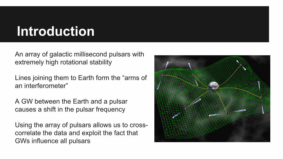
IntroductionAn array of galactic millisecond pulsars with extremely high rotational stability
Lines joining them to Earth form the “arms of an interferometer”
A GW between the Earth and a pulsar causes a shift in the pulsar frequency
Using the array of pulsars allows us to cross-correlate the data and exploit the fact that GWs influence all pulsars
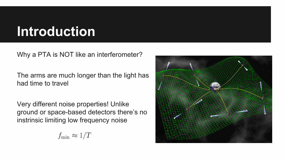
IntroductionWhy a PTA is NOT like an interferometer?
The arms are much longer than the light has had time to travel
Very different noise properties! Unlike ground or space-based detectors there’s no instrinsic limiting low frequency noise
Sources of GWs
Or a lower mass binary in the earlier stages of inspiral.
The main source of GWs in this frequency band is thought to be a population of supermassive black hole binaries, with typical masses and redshifts , in the early inspiral regime of their coalescence
As you move to lower frequencies there are more binaries per frequency bin and they superpose to form a stochastic background
Sources of GWs
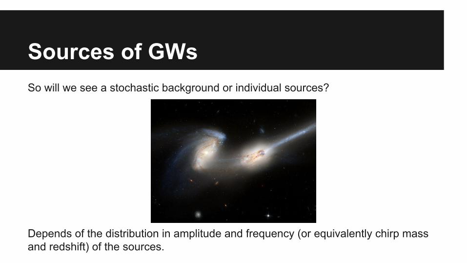
Sources of GWsSo will we see a stochastic background or individual sources?
Depends of the distribution in amplitude and frequency (or equivalently chirp mass and redshift) of the sources.
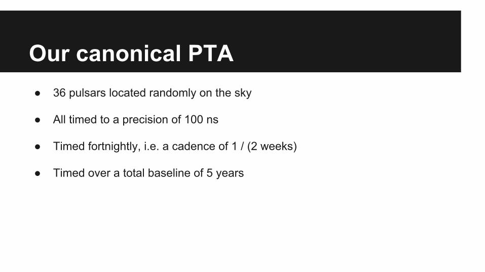
Our canonical PTA● 36 pulsars located randomly on the sky
● All timed to a precision of 100 ns
● Timed fortnightly, i.e. a cadence of 1 / (2 weeks)
● Timed over a total baseline of 5 years
Roughly equivalent to of the IPTA mock data challenge

Our canonical PTA● 36 pulsars located randomly on the sky
● All timed to a precision of 100 ns
● Timed fortnightly, i.e. a cadence of 1 / (2 weeks)
● Timed over a total baseline of 5 years
Roughly equivalent to of the IPTA mock data challenge

IPTA pulsar locationsJ0030+0451 J0218+4232J0437-4715 J0613-0200 J0621+1002 J0711-6830 J0751+1807 J0900-3144 J1012+5307 J1022+1001J1024-0719 J1045-4509 J1455-3330 J1600-3053 J1603-7202 J1640+2224J1643-1224 J1713+0747J1730-2304 J1732-5049 J1738+0333 J1741+1351 J1744-1134 J1751-2857 J1853+1303 J1857+0943 J1909-3744 J1910+1256J1918-0642 J1939+2134 J1955+2908 J2019+2425 J2124-3358 J2129-5721 J2145-0750 J2317+1439

Sensitivity curves
Interactive version of figure online at

Sensitivity curves
?
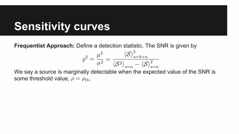
Sensitivity curvesFrequentist Approach: Define a detection statistic. The SNR is given by
We say a source is marginally detectable when the expected value of the SNR is some threshold value, .
Bayesian Approach: Calculate the evidence for two competing hypotheses. Bayes factor.
We say a source is marginally detectable when the expected Baye’s factor is some threshold value, .

Sensitivity curvesFrequentist Approach: Define a detection statistic. The SNR is given by
We say a source is marginally detectable when the expected value of the SNR is some threshold value, .
Bayesian Approach: Calculate the evidence for two competing hypotheses, the noise and signal hypothesis. The Bayes’ factor is the ratio
We say a source is marginally detectable when the expected Bayes’ factor is some threshold value, .

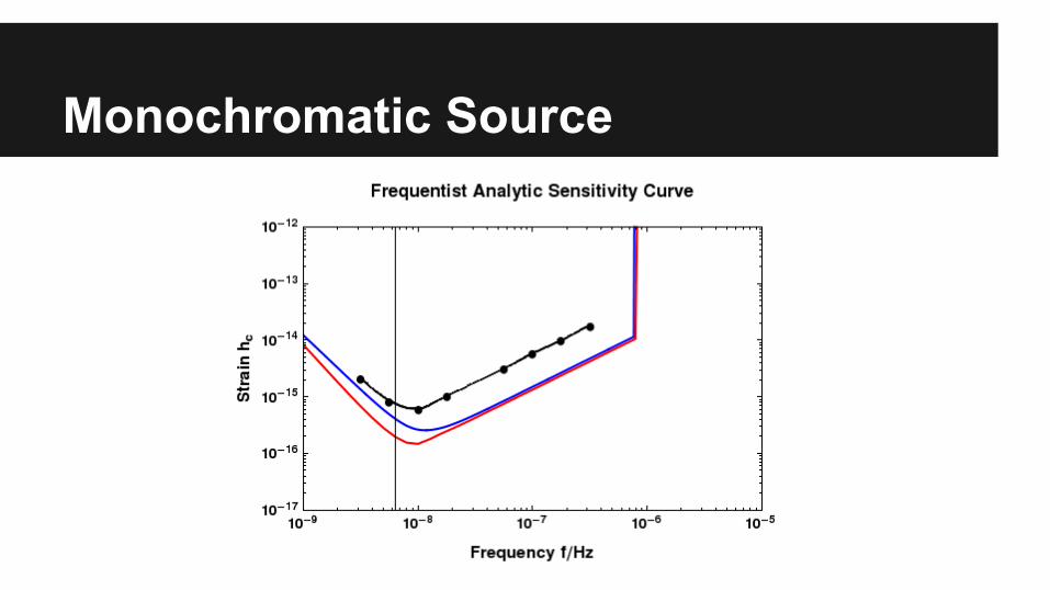
Monochromatic SourceFrequentist approach:
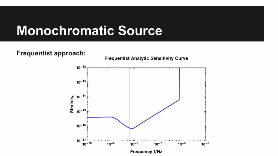
Monochromatic SourceFrequentist approach:

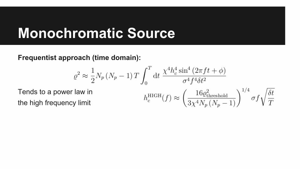
Frequentist approach (time domain):
Tends to a power law in the high frequency limit
Also a power law inthe low frequency limit
Monochromatic Source
0 0 0
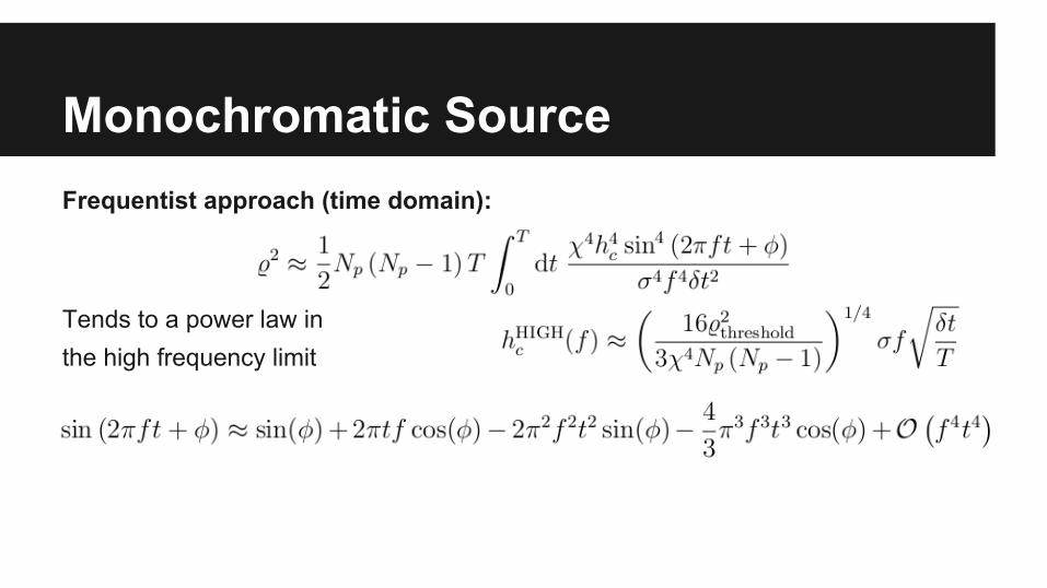
Frequentist approach (time domain):
Tends to a power law in the high frequency limit
Also a power law inthe low frequency limit
Monochromatic Source
0 0 0
Frequentist approach (time domain):
Tends to a power law in the high frequency limit
Also a power law inthe low frequency limit
Monochromatic Source

Frequentist approach (time domain):
Tends to a power law in the high frequency limit
Also a power law inthe low frequency limit
Monochromatic Source
0Distance
Frequentist approach (time domain):
Tends to a power law in the high frequency limit
Also a power law inthe low frequency limit
Monochromatic Source
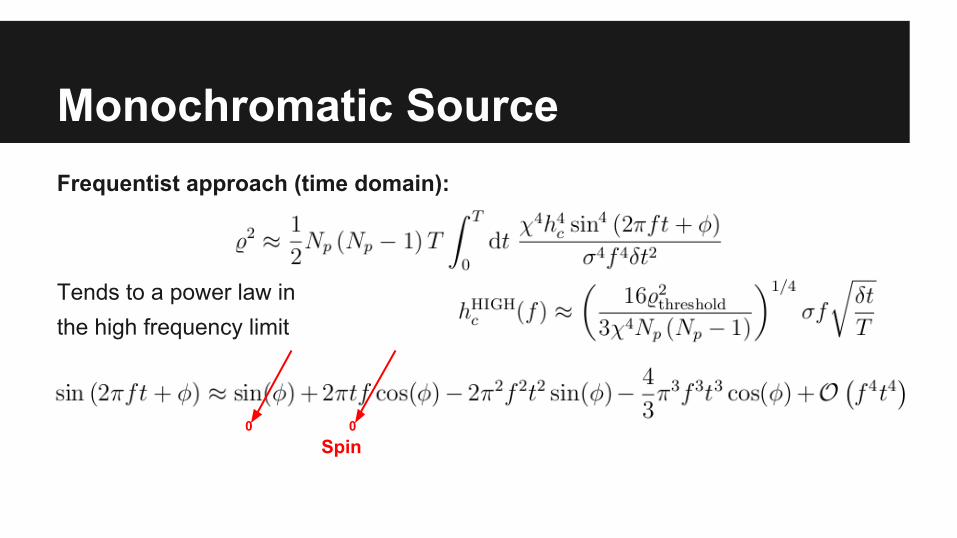
0Spin
0

Frequentist approach (time domain):
Tends to a power law in the high frequency limit
Also a power law inthe low frequency limit
Monochromatic Source
0 0 0Spin-down

Frequentist approach (time domain):
Tends to a power law in the high frequency limit
Also a power law inthe low frequency limit
Monochromatic Source
0 0 0

Frequentist approach (time domain):
Monochromatic Source

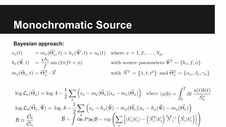
Bayesian approach:
Monochromatic Source
Bayesian approach:
Monochromatic Source
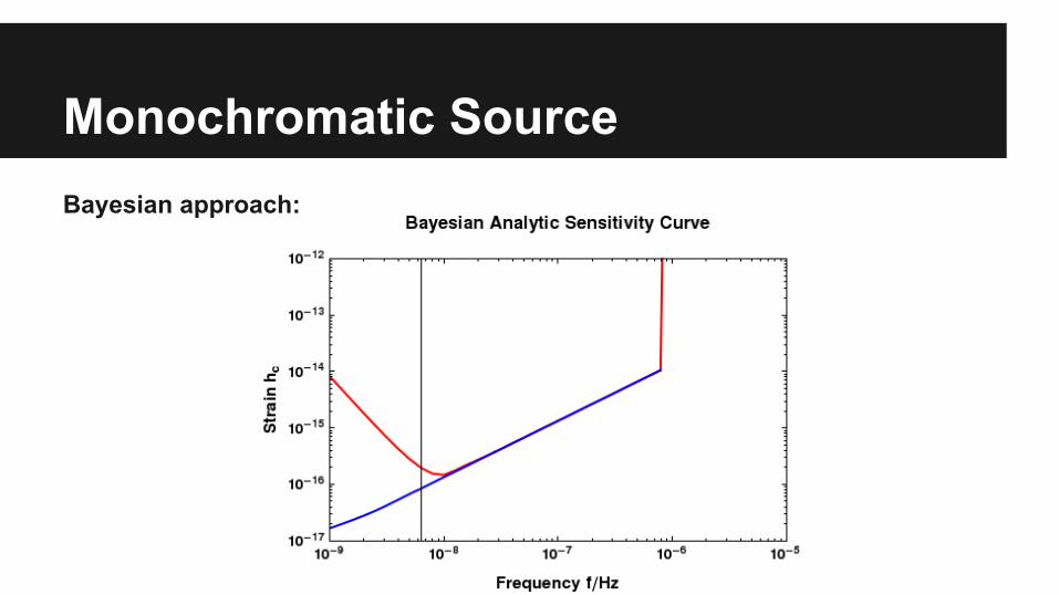
Monochromatic SourceBayesian approach:
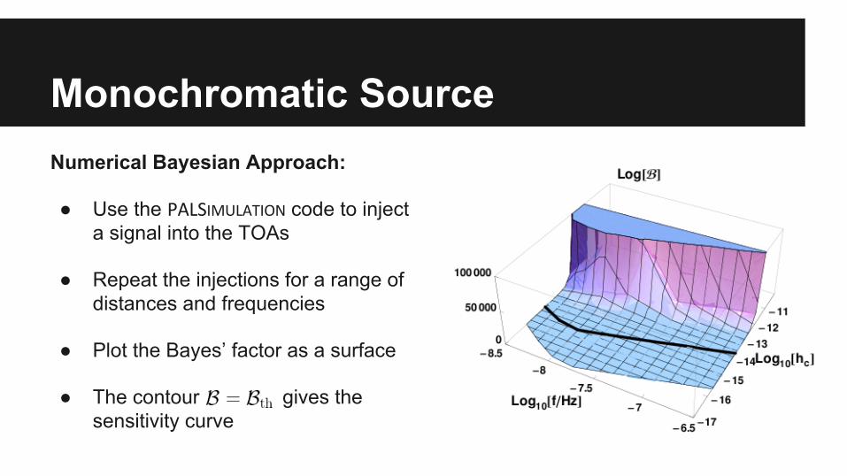
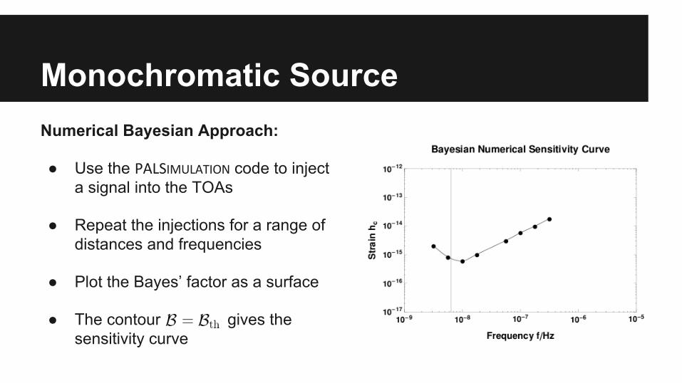
Monochromatic SourceNumerical Bayesian Approach:
● Use the code to inject a signal into the TOAs
● Repeat the injections for a range of distances and frequencies
● Plot the Bayes’ factor as a surface
● The contour gives the sensitivity curve
Monochromatic SourceNumerical Bayesian Approach:
● Use the code to inject a signal into the TOAs
● Repeat the injections for a range of distances and frequencies
● Plot the Bayes’ factor as a surface
● The contour gives the sensitivity curve

Monochromatic Source
Monochromatic Source

Monochromatic Source

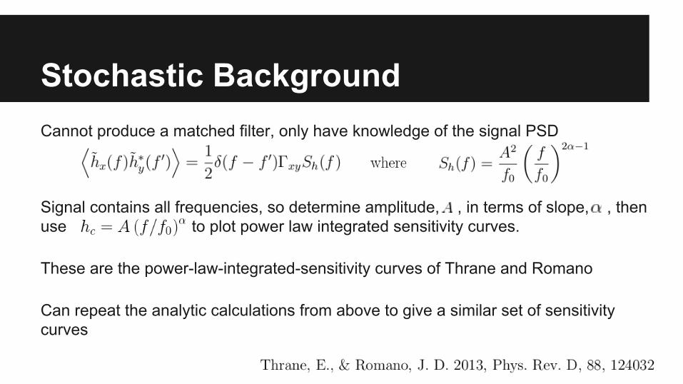
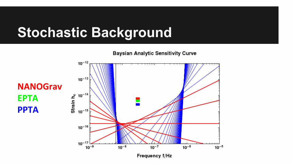
Stochastic BackgroundCannot produce a matched filter, only have knowledge of the signal PSD
Signal contains all frequencies, so determine amplitude, , in terms of slope, , then use to plot power law integrated sensitivity curves.
These are the power-law-integrated-sensitivity curves of Thrane and Romano
Can repeat the analytic calculations from above to give a similar set of sensitivity curves
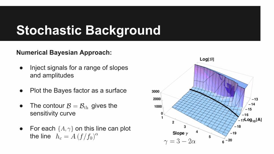
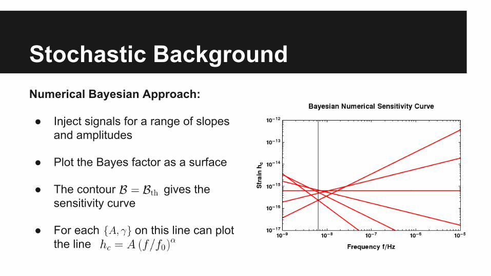
Stochastic BackgroundNumerical Bayesian Approach:
● Inject signals for a range of slopes and amplitudes
● Plot the Bayes factor as a surface
● The contour gives the sensitivity curve
● For each on this line can plot the line
Stochastic BackgroundNumerical Bayesian Approach:
● Inject signals for a range of slopes and amplitudes
● Plot the Bayes factor as a surface
● The contour gives the sensitivity curve
● For each on this line can plot the line
Stochastic Background
Stochastic Background
Conclusions
● The sensitivity curve depends on the properties of the source and the detector
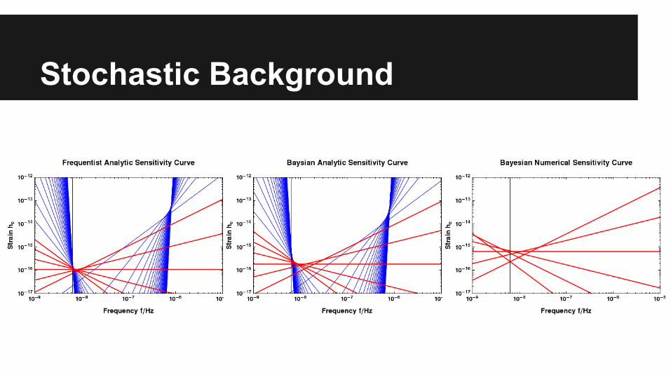
● The shape of the sensitivity curve can be understood using simple analytic arguments in either a Bayesian or frequentist approach
● The different approaches were found to be in good agreement and also in agreement with the numerical calculations
Top Related