


Languages
Pages
Legal

THE INFLUENCE OF MACROECONOMIC FACTORS
TOWARD GROSS DOMESTIC PRODUCT OF
INDONESIA FOR PERIOD 1981 – 2015
By:
Morinnalia Isadora
014201300111
A Skripsi presented to the
School of Business President University
in partial fulfillment of the requirements for
Bachelor Degree in Economics Major in Management
December 2016

i
PANEL OF EXAMINERS
APPROVAL SHEET
The Panel of Examiners declare that the skripsi entitled “THE INFLUENCE OF
MACROECONOMIC FACTORS TOWARD GROSS DOMESTIC
PRODUCT OF INDONESIA FOR PERIOD 1981 - 2015” that was submitted
by Morinnalia Isadora majoring in Management from School of Business was
assessed and approved to have passed the Oral Examinations on December 16th
2016.
Dr. Ir. Yunita Ismail Masjud, MSi
Chair – Panel of Examiners
Dr. Dra. Genoveva, MM
Examiner 1
Filda Rahmiati, MBA
Examiner 2
ii
SKRIPSI ADVISER
RECOMMENDATION LETTER
This skripsi entitled “THE INFLUENCE OF MACROECONOMIC
FACTORS TOWARD GROSS DOMESTIC PRODUCT OF INDONESIA
FOR PERIOD 1981 - 2015” prepared and submitted by Morinnalia Isadora in
partial fulfillment of the requirements for the degree of Bachelor in the School of
Business has been reviewed and found to have satisfied the requirement for a
skripsi fit to be examined. I therefore recommend this skripsi for Oral Defense.
Cikarang, Indonesia, December 9th
, 2016
Acknowledged by, Recommended by,
Dr. Dra. Genoveva, MM Filda Rahmiati, MBA
Head of Management Study Program Skripsi Advisor

iii
DECLARATION OF ORIGINALITY
I declare that this skripsi, entitled “THE INFLUENCE OF
MACROECONOMIC FACTORS TOWARD GROSS DOMESTIC
PRODUCT OF INDONESIA FOR PERIOD 1981 - 2015” is, to be the best of
my knowledge and belief, and original piece of work that has not been submitted,
either in a whole or in a part, to another university to obtain a degree.
Cikarang, Indonesia, December 9th
, 2016
Morinnalia Isadora
iv
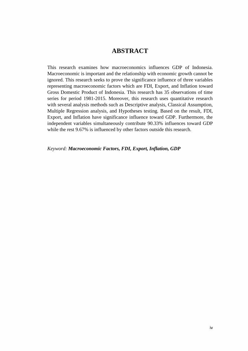
ABSTRACT
This research examines how macroeconomics influences GDP of Indonesia.
Macroeconomic is important and the relationship with economic growth cannot be
ignored. This research seeks to prove the significance influence of three variables
representing macroeconomic factors which are FDI, Export, and Inflation toward
Gross Domestic Product of Indonesia. This research has 35 observations of time
series for period 1981-2015. Moreover, this research uses quantitative research
with several analysis methods such as Descriptive analysis, Classical Assumption,
Multiple Regression analysis, and Hypotheses testing. Based on the result, FDI,
Export, and Inflation have significance influence toward GDP. Furthermore, the
independent variables simultaneously contribute 90.33% influences toward GDP
while the rest 9.67% is influenced by other factors outside this research.
Keyword: Macroeconomic Factors, FDI, Export, Inflation, GDP

v
ACKNOWLEDGEMENT
Through this opportunity, I would like to thank to God who always gave me
blessing and strength to finish this skripsi. Through this opportunity, I would like
to show my gratitude to the following people:
1. Researcher‟s beloved family, especially Mom, Dad, and brother who
always give the unlimited supports, love, blessings and prayers for me.
2. Researcher‟s skripsi advisor, Filda Rahmiati, BBa, MBA. Thank you so
much for the kindness, guidance, attention, and patience. I am so honored
and grateful to have you as skripsi advisor and lecturer.
3. Orlando Santos MBA, Rosita Widjojo, Dr. Dra. Genoveva, MBA, MM,
Marie Ann C, MBA, and the other President University lecturers who have
taught researcher so many knowledge and give so many advices during
these study times. Thank you so much for your care, time, and kindness,
you guys are so cool!
4. My best friends, Rosalia and Vivi Lorensa. Thank you for always being
my caring and supporting friends. You are awesome girls!
5. My comrade, David Willy Otniel, Viona Devi Anbielica, Aris Akbar,
Vivian Noreen, Florencia Irene Chang. Thank you for the crazy time we
shared together through the laugh and struggle.
6. The juniors-like-siblings, Elviny Edison, Joselind Agusta Pratama,
Richard Keane, Ade Dwi Septiani, Gweneal Benita, and others who have
supported and cared. Thank you for your jokes, stories, and craziness.
7. To those who indirectly contributed in this research, your kindness means
a lot. Thank you very much.
8. All of Management students who have shared many experiences through
years in university, I hope we can be impactful person with moral and
value in the future.

vi
The researcher fully realized that this skripsi is still far for perfection, but always
hope that this skripsi can be helpful for anyone who need it. Researcher hoped this
skripsi can give positive contribution to the readers.
Best Regards,
Morinnalia Isadora

vii
TABLE OF CONTENTS
PANEL OF EXAMINERS APPROVAL SHEET ............................................... i
SKRIPSI ADVISER RECOMMENDATION LETTER ................................... ii
DECLARATION OF ORIGINALITY .............................................................. iii
ABSTRACT .......................................................................................................... iv
ACKNOWLEDGEMENT .................................................................................... v
TABLE OF CONTENTS .................................................................................... vii
LIST OF TABLES ................................................................................................ x
LIST OF FIGURES .............................................................................................. x
LIST OF EQUATIONS ....................................................................................... xi
CHAPTER I ........................................................................................................... 1
1.1. Background ............................................................................................. 1
1.2. Need of the Study .................................................................................... 5
1.3. Problem Identification ........................................................................... 5
1.4. Research Questions ................................................................................ 6
1.5. Research Objectives ............................................................................... 7
1.6. Significance of Study .............................................................................. 7
1.7. Scope & Limitation ................................................................................ 8
1.8. Organization of the Skripsi ................................................................... 8
CHAPTER II ....................................................................................................... 10
2.1. Introduction .......................................................................................... 10
2.2. Gross Domestic Product....................................................................... 10
2.3. FDI .............................................................. Error! Bookmark not defined.
2.4. Exports .................................................................................................. 12
2.5. Inflation ................................................................................................. 13
2.6. Research Gap ........................................................................................ 14
CHAPTER III ..................................................................................................... 16
3.1. Introduction .......................................................................................... 16
3.2. Theoretical Framework ....................................................................... 16
3.3. Hypotheses ............................................................................................ 17
3.4. Operational Definitions of variables ................................................... 18

viii
3.5. Research Instrument ............................................................................ 18
3.6. Sampling ................................................................................................ 19
3.6.1. Population ...................................................................................... 19
3.6.2. Sampling Technique ..................................................................... 19
3.6.3. Sample ............................................................................................ 19
3.6.4. Data Collection Method ................................................................ 20
3.6.5. Data Analysis Method ................................................................... 20
3.6.5.1. Descriptive Statistic Analysis.................................................... 20
3.6.5.2. Stationarity Test ........................................................................ 20
3.6.5.3. Multiple Regression Test .......................................................... 20
3.6.5.4. Classical Assumption Test ........................................................ 21
3.6.5.5. Hypothesis Testing .................................................................... 23
CHAPTER IV ...................................................................................................... 25
4.1. Data Analysis ........................................................................................ 25
4.1.1. Descriptive Statistive Result ......................................................... 25
4.1.2. Normality of the Data ................................................................... 26
4.1.3. Stationarity Test ............................................................................ 27
4.1.4. Multiple Regression Model .......................................................... 27
4.1.5. Classical Assumption .................................................................... 28
4.1.5.1. Normality Test ........................................................................... 28
4.1.5.2. Heteroscedsticity Test ............................................................... 29
4.1.5.3. Multicollinearity Test ................................................................ 30
4.1.5.4. Autocorrelation Test ................................................................. 30
4.2. Hypothesis Testing ............................................................................... 31
4.2.1. T-Test ............................................................................................. 31
4.2.2. F-Test .............................................................................................. 32
4.3. Interpretation of Result ....................................................................... 33
4.3.1. Influence of FDI towards GDP .................................................... 33
4.3.2. Influence of Export towards GDP ............................................... 34
4.3.3. Influence of Inflation towards GDP ............................................ 34
4.3.4. Simultaneous Influence Factors ................................................... 35
CHAPTER V ....................................................................................................... 36
5.1. Conclusion ............................................................................................. 36

ix
5.2. Future Recommendation ..................................................................... 37
5.2.1. For Government ............................................................................ 37
5.2.2. For Future Researcher ................................................................. 38
REFERENCES .................................................................................................... 39
APPENDICES ..................................................................................................... 42
x
LIST OF TABLES
Table 4.1 Descriptive Statistic Result....................................................... 26
Table 4.2 Stationarity Test Result........................................………......... 28
Table 4.3 Multiple Regression Model Result.......……………………….. 28
Table 4.4 Normality Test Result........................…………………………. 30
Table 4.5 Heteroscedasticity Test: Glejser Result...............………….… 30
Table 4.6 Multicollinearity Test Result...................................................... 31
Table 4.7 Durbin-Watson Test Result.....................................………....... 32
Table 4.8 F-Test Result................................................................................ 33
Table 4.9 Coefficient of Determination (R2) Result.................................. 34
Table 4.10 Summary of Analysis.................................................................. 36
LIST OF FIGURES
Figure 1.1 Gross Domestic Product of Indonesia…………………….... 2
Figure 1.2 Gross Domestic Product Growth of Indonesia...................... 3
Figure 1.3 FDI Inflow of Indonesia.....….....…... 4
Figure 1.4 Annual Inflation Rate of Indonesia...............…………........ 5
Figure 3.1 Research Framework ……………………………………...... 17
Figure 4.1 Normality Test of the Data …………………………………. 27

xi
LIST OF EQUATIONS
Equation 1. Gross Domestic Product …………………………………... 11
Equation 2. Multiple Regression ………………………………...……... 21
Equation 3. Multiple Regression Result……………………………...… 29
1
CHAPTER I
INTRODUCTION
1.1. Background
Indonesia is the fourth most populous country in the world with 257,563,815 as
per 2015 following China, India, and the United States (World Bank, 2016). There
are 13,446 islands in Indonesia‟s territory, make Indonesia archipelago country
(Worldometers, 2016). On the other hand, a report released by World Economic
Forum that Indonesia secures 42nd place out 60 lists in the best country in the
world (Time, 2016). That was achieved from the overall view of economic
situations in the country.
According to Karya & Syamsuddin (2016) Gross Domestic Product (GDP) is the
output that produced in a country by both its people and not, as long as the goods
and services are produced within the country. GDP is the total amount of final
produced goods and services, by the circular flow principle, it is equal to the total
income earned through domestically located production and also equal to total
expenditure on goods and services that domestically produced (DeLong & Olney,
2006).
GDP can be calculated in a certain time period, and usually it is calculated
annually. According to Coyle (2014) GDP is a measurement of nation‟s overall
economic activity and commonly used as indicator of economic health. GDP of
Indonesia is shown in Figure 1.1. The figure shows the GDP of Indonesia is
increasing steadily from 1981, however it fall in 1998 and since 2002 it keep
rising until 2012, starting from 2013 the GDP of Indonesia keep falling until 2015.

2
Figure 1.1 Gross Domestic Product of Indonesia
Source: World Bank, 2016
Nasrullah (2014) stated that economic growth is an important phenomenon of a
country that it will influence the life quality of its people. To develop a country
and its people, a country needs labor, technology, and capital. The educated and
skilled labor is needed to do the job while the equipment and technology is needed
to equip the labor. On the other hand, capital can be received from investment.
Foreign Direct Investment (FDI) brings capital and technology to the host country,
it is important for the developing country to be able to have the access to advance
technology.
According to Simpson (2014), macroeconomic is one of important aspects that
driven the country and the prosperity of the citizens. Asian crisis in 1998 was one
of the worst conditions to the impacted countries such as Indonesia, Thailand, and
South Korea. Indonesia especially suffered from currency crisis, banking crisis,
and debt crisis. According to Bank Indonesia (2016), comparing the other
impacted countries, Indonesia suffered longer and worse because of the unstable
political condition. Followed by financial crisis in 2008 that triggered by America
and impacted to the global economic. As the impact to Indonesia, many foreign
investors disinvest from Indonesia lead to the weakened of Rupiah. Compared to
the other Asia countries such as Malaysia and Singapore, Indonesia was less
0
200.000
400.000
600.000
800.000
1.000.000
19
81
19
84
19
87
19
90
19
93
19
96
19
99
20
02
20
05
20
08
20
11
20
14
Mill
ion
USD
GDP of Indonesia
Indonesia

3
impacted because the value of Export was considered small compared to others
(Bank Indonesia, 2016).
During the crisis in 1998, the value of Indonesian GDP fall sharply from 215.749
billion USD in 1997 to 95.446 billion USD in 1998 as can be seen in Figure 1.1.
Meanwhile, GDP Growth of Indonesia can be seen in Figure 1.2, year 1998
marked to be the greatest fall out of Indonesian history with -13.127 percent GDP
growth. Thailand that suffered from the crisis also reached the bottom with -7.634
percent. Indonesia fall more than Thailand in 1998 and recover slower in the next
year. Thailand was able to recover to 4,572 percent in the next year, while
Indonesia recovered slowly to 0.791 percent in 1999 (World Bank, 2016).
Figure 1.2 Gross Domestic Product Growth of Indonesia
Source: World Bank, 2016
Following crisis in 1998, there was global crisis affected Indonesia at the end of
2008. Domestic currency in 1998 weakened to 9,698.963 from 9,141 in the
previous year, it lead to the fall of export value and Indonesian GDP growth fall to
6.014 percent in 2008 and impacted to the fall to 4.629 percent in 2009, as it is
shown in Figure 1.2. Similar to 1998, the crisis in 2008 brought fall to FDI in
2009, however it recovered quickly. Ever since 2012, Indonesia suffers economic
-15
-10
-5
0
5
10
1995 1997 1999 2001 2003 2005 2007 2009 2011 2013 2015
Pe
rce
nt
(%)
GDP Growth
Indonesia

4
slowdown caused by global condition such as the increase of interest rate, Greece
economic crisis, depreciation of Chinese Yuan, Greece (Merdeka, 2015).
As the impact of crisis, Indonesian currency weakened greatly, the value of
Indonesian Rupiah against USD was 2,909.380 in 1997 and it skyrocketed to
10,013.623 in 1998 when the Indonesia faced the crisis. A year later in 1999,
Rupiah strengthened to 7,855.150. However Rupiah were fluctuated and have
never gone back to the level of 2,909.380 ever since 1998 (World Bank, 2016).
Moreover, FDI of Indonesia has fallen several times as the impact of crisis. The
crisis in 1998 left Indonesia with -240,800,000 USD of FDI Inflow and in became
worse in the following years. FDI Inflow in 1999 was -1,866,000,000 and in 2000
it fall to -4,550,000,000. The data are shown in Figure 1.3. The unstable political
condition triggered disinvestment in Indonesia, and the value reached minus when
disinvestment is greater than investment (World Bank, 2016).
Figure 1.3 FDI Inflow of Indonesia
Source: World Bank, 2016
As the up and down of a country economic, the live of the people is influenced
(Karya & Syamsuddin, 2016). Inflation Rate can be seen in Figure 1.4.
Indonesia‟s Inflation rate in 1997 was 6.23 percent exploded to 58.387 percent
annually in 1998 and monthly inflation skyrocketed to more than 80 percent in
September 1998, marked Indonesia as a country suffered in Hyperinflation
(Inflation.eu, 2016). Thailand Inflation rate increase slightly from 5.626 percent in
-10.000.000.000
0
10.000.000.000
20.000.000.000
30.000.000.000
US
Do
llar
Foreign Direct Investment Inflow
Indonesia

5
1997 to 7.995 percent in 1998 and fall sharply to 0.285 in 1999, ever since then
there were a slight fluctuation. According to Karya & Syamsuddin (2016) the
hyperinflation brought misery to people along with the quality of education fell,
the quality of healthyness fell. From Figure 1.4, can be seen the value of Inflation
is increase from 4.29% in 2012 to to the point of 6.413 in 2013 and it stabel in
±6% for the next couple years, 6.395% in 2014 and 6.363% in 2015.
Figure 1.4 Annual Inflation Rate of Indonesia
Source: World Bank, 2016
1.2. Need of the Study
The need of this research is to examine the influence of Macroeconomic Factors
which are represented by FDI, Export, and Inflation toward Gross Domestic
Product of Indonesia.
1.3. Problem Identification
As shown by Figure 1.4. in the background of study, it is indicated that Indonesia
has an unstable Inflation rate and had suffered from hyperinflation in the 1998. In
-10
0
10
20
30
40
50
60
19
81
19
83
19
85
19
87
19
89
19
91
19
93
19
95
19
97
19
99
20
01
20
03
20
05
20
07
20
09
20
11
20
13
20
15
Pe
rce
nt
(%)
Inflation
Indonesia
6
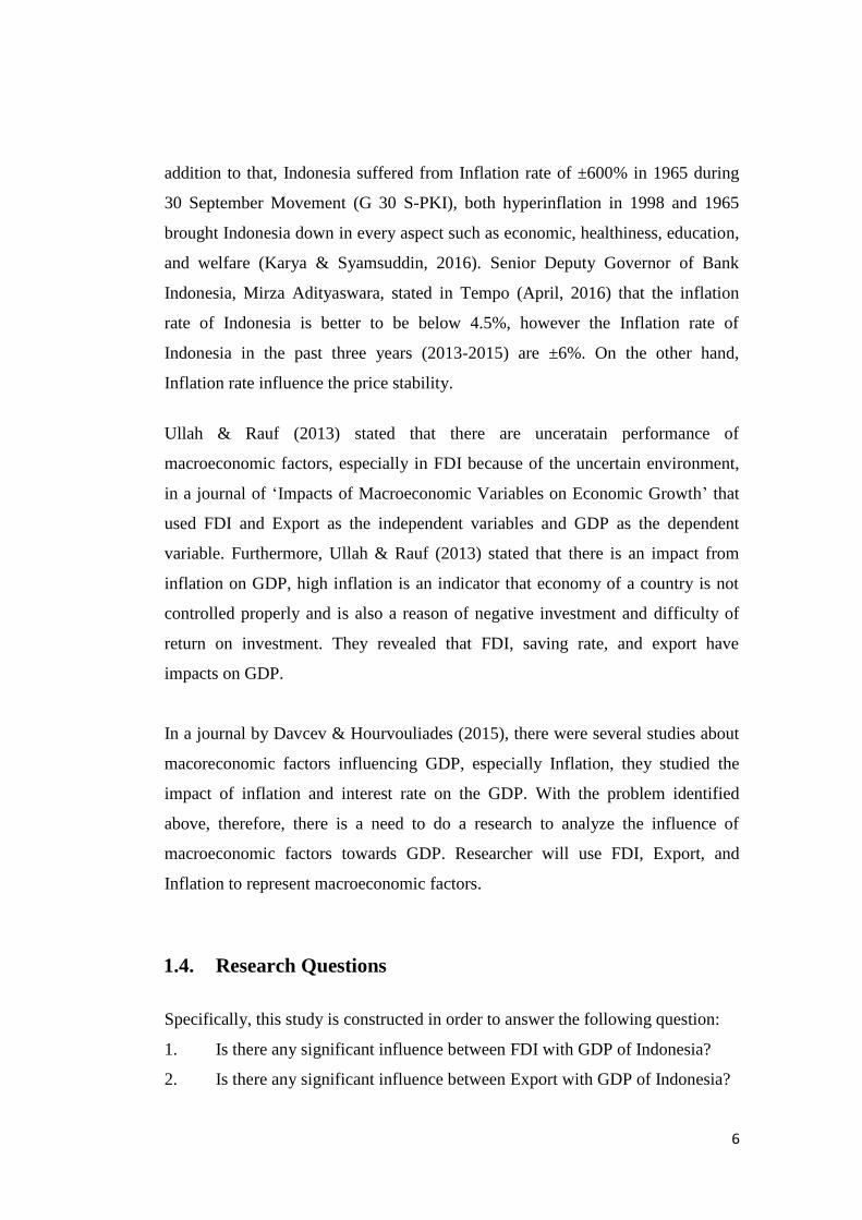
addition to that, Indonesia suffered from Inflation rate of ±600% in 1965 during
30 September Movement (G 30 S-PKI), both hyperinflation in 1998 and 1965
brought Indonesia down in every aspect such as economic, healthiness, education,
and welfare (Karya & Syamsuddin, 2016). Senior Deputy Governor of Bank
Indonesia, Mirza Adityaswara, stated in Tempo (April, 2016) that the inflation
rate of Indonesia is better to be below 4.5%, however the Inflation rate of
Indonesia in the past three years (2013-2015) are ±6%. On the other hand,
Inflation rate influence the price stability.
Ullah & Rauf (2013) stated that there are unceratain performance of
macroeconomic factors, especially in FDI because of the uncertain environment,
in a journal of „Impacts of Macroeconomic Variables on Economic Growth‟ that
used FDI and Export as the independent variables and GDP as the dependent
variable. Furthermore, Ullah & Rauf (2013) stated that there is an impact from
inflation on GDP, high inflation is an indicator that economy of a country is not
controlled properly and is also a reason of negative investment and difficulty of
return on investment. They revealed that FDI, saving rate, and export have
impacts on GDP.
In a journal by Davcev & Hourvouliades (2015), there were several studies about
macoreconomic factors influencing GDP, especially Inflation, they studied the
impact of inflation and interest rate on the GDP. With the problem identified
above, therefore, there is a need to do a research to analyze the influence of
macroeconomic factors towards GDP. Researcher will use FDI, Export, and
Inflation to represent macroeconomic factors.
1.4. Research Questions
Specifically, this study is constructed in order to answer the following question:
1. Is there any significant influence between FDI with GDP of Indonesia?
2. Is there any significant influence between Export with GDP of Indonesia?
7
3. Is there any significant influence between Inflation with GDP of
Indonesia?
4. Is there any simultaneously significant influence of FDI, Exchange Rate
and Inflation with GDP of Indonesia?
1.5. Research Objectives
According to the preceding research questions, the research objectives of the
study can be translated as follows:
1. To find out if there is significant influence between FDI with GDP of
Indonesia.
2. To find out if there is significant influence between Export with GDP of
Indonesia.
3. To find out if there is significant influence between Inflation with GDP of
Indonesia.
4. To find out if there is simultaneously significant influence between FDI,
Exchange Rate and Inflation with GDP of Indonesia.
1.6. Significance of Study
Through this research hopefully could expand knowledge, information, and
suggestion for:
1.6.1. Researcher
This research is partial fulfillment of requirement for the researcher to obtain
bachelor degree. However, this research will definitely give valuable experiences
for researcher in conducting a research especially in implementing international
business theories, especially in macroeconomic. In addition from the technical
point of view, researcher will gain knowledge deeply about how to conduct a
research in a right way.
8
1.6.2. Government
The result of this research hopefully could be a contribution or suggestion on
determining the policy of economic development in Indonesia.
1.6.3. The University
The result of research is expected to be useful for academic purpose of President
University students in particular for Management students concentrated in
International Business and it will contribute the literatures and studies in field of
Economic in terms of macroeconomic.
1.6.4. Future Researcher
The result of this research could be used as a baseline for the next research about
macroeconomic of Indonesia, especially in GDP.
1.7. Scope & Limitation
1.7.1. Scope
This research is conducted by analyzing the influence of macroeconomic factors
which is represented by FDI, Export, and Inflation toward GDP of Indonesia.
1.7.2. Limitation
This research focuses on the influence of macroeconomic factors which are FDI,
Export, and Inflation toward GDP of Indonesia for the period of 1981 to 2015.
The country used in this research will be a country part of South East Asia that
had suffered from hyperinflation and the GDP is decreasing in the past few years
which is Indonesia.
1.8. Organization of the Skripsi
This research consists of five chapters, which are Introduction, Literature Review,
Methodology, Data Analysis and Conclusion. Chapter 1 provides the overview of

9
entire research study which contains research background and the need for study
followed by problem statement, research questions and objectives, significance of
the study, limitation and organization of thesis. Chapter 2 provides review of
literature on each variable and research gap. Chapter 3 consists of research
framework, hypotheses, operational definitions, research design and sampling
plan. Chapter 4 consists of descriptive analysis, inferential analysis and
discussions. The last but not least is Chapter 5, which consists of conclusion of
this research.

10
CHAPTER II
LITERATURE REVIEW
2.1. Introduction
This chapter is focused not only on both dependent and independent variables, but
how independent variables influence dependent variable and the research gap. The
dependent variable is GDP and independent variables are FDI, Export and
Inflation.
2.2. Gross Domestic Product
Gross Domestic Product (GDP) is the most commonly used to measure output,
income, and the product, also is the total amount of final goods and services
produced according to Delong & Olney (2006). One contribution from Adam
Smith is that he recognized the importance of free trade and labor exchange as a
mechanism of economic growth (Karya & Syamsuddin, 2016). Through „The
Wealth of Nations‟ in 1776, Adam Smith created Gross Domestic Product concept
that countries should be calculated according to their production and commerce,
where the wealth of a country is measured by gold and silver deposit before.
This research uses GDP as the dependent variable because whenever there is an
increase in GDP, it will raise the overall output and it called economic growth
(Ullah and Rauf, 2013). In addition, Abdu (2013) stated that economic growth is
the growth in real terms of GDP in a given year. Economies grow as a result of
several factors, however GDP growth is the most critical because it symbolizes
the output of domestic industries, it creates employment and wealth. GDP is a
measurement of a final value of goods and services produced in a period of time.
The equation of GDP is as follow.
11
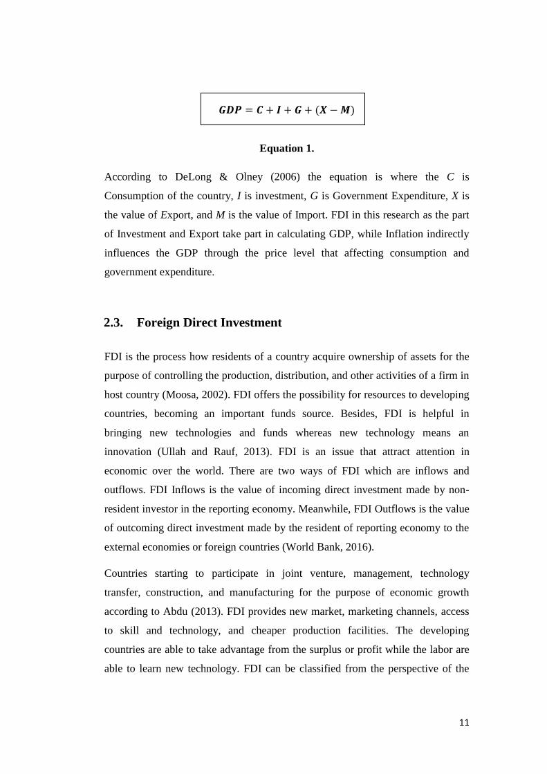
𝑮𝑫𝑷 = 𝑪 + 𝑰 + 𝑮 + (𝑿 −𝑴)
Equation 1.
According to DeLong & Olney (2006) the equation is where the C is
Consumption of the country, I is investment, G is Government Expenditure, X is
the value of Export, and M is the value of Import. FDI in this research as the part
of Investment and Export take part in calculating GDP, while Inflation indirectly
influences the GDP through the price level that affecting consumption and
government expenditure.
2.3. Foreign Direct Investment
FDI is the process how residents of a country acquire ownership of assets for the
purpose of controlling the production, distribution, and other activities of a firm in
host country (Moosa, 2002). FDI offers the possibility for resources to developing
countries, becoming an important funds source. Besides, FDI is helpful in
bringing new technologies and funds whereas new technology means an
innovation (Ullah and Rauf, 2013). FDI is an issue that attract attention in
economic over the world. There are two ways of FDI which are inflows and
outflows. FDI Inflows is the value of incoming direct investment made by non-
resident investor in the reporting economy. Meanwhile, FDI Outflows is the value
of outcoming direct investment made by the resident of reporting economy to the
external economies or foreign countries (World Bank, 2016).
Countries starting to participate in joint venture, management, technology
transfer, construction, and manufacturing for the purpose of economic growth
according to Abdu (2013). FDI provides new market, marketing channels, access
to skill and technology, and cheaper production facilities. The developing
countries are able to take advantage from the surplus or profit while the labor are
able to learn new technology. FDI can be classified from the perspective of the

12
investor and host country. According to Elia et al. (2013), types of FDI from the
perspective of investor are as follow:
1. Horizontal FDI
The investor produces the same or similar kinds of goods (in the same industry) in
the host country as in the home country such as Toyota that assembling cars in
both Japan as the home country and Indonesia as the host country.
2. Vertical FDI
The investor invests in different stages in the same industry. There are two types
of Vertical FDI, which are Forward Vertical and Backward Vertical. Backward
Vertical is where the investor moves back towards the raw materials, fulfilling the
role of supplier. Whereas, Forward Vertical is where it takes the investor closer to
the market and acquire the role of distributor such as Toyota acquires car
distributor in Indonesia.
3. Conglomerate FDI
Conglomerate FDI happens when the investor invests in a new unrelated business
with the previous business in host country.
The relationship between FDI and economic growth according to Abdu (2013) is
significantly influenced. In the study, it stated that stability of FDI can stimulate
product diversification through investment into new business. In addition, it
expands business and able to improve employment and raise wages. However,
these benefits are only for some people, such as the employee training limited to
some groups.
2.4. Exports
In macroeconomic theory, a relation between export and economic growth or
GDP is an equation since export is part of national income (Nasrullah, 2014). As a
part of national income, where it is an international trading system that one send

13
goods and services to another country for sale according to the applied conditions.
However, the higher the number of export, the more the country will be sensitive
to the fluctuation in the international market or the world economy (Nasrullah,
2014). Export is influenced by supply and demand of the goods and services.
Demand influences export through the prices, exchange rate, and devaluation
policy. On the other hand, supply influences export through production capacity,
investment, raw material, and deregulation policy.
According to Seyoum (2014) in the book of Export Import Theory, Practices, and
Procedure, international trade played an important role in the economic
development of North America and Australia in the nineteenth century and East
Asian in the twentieth century. While the new prosperity was shared among the
population, East Asia‟s growth leads to increased living standards and reduced
inequality. In addition, Thailand and Malaysia able to reduced poverty from
almost 50% in 1960s to less than 20% by 2000. All of this success is caused by
export, where the government provided the credits, developed export marketing
institutions and restricted competing imports. As the result, the economic grew
about 7 percent per year.
Export of a country is important factor that may affect economic growth.
According to Ullah and Rauf (2013) more exports mean more allocation of
resources and more utilization of resources means more production.
2.5. Inflation
Inflation is understood as an ongoing rise across a broad spectrum of prices.
Meanwhile, an increase in price of one or two goods cannot be described as
inflation unless that increase lead to other goods (Bank Indonesia, 2016).
According to Ullah and Rauf (2013) there are strong arguments that support
inflation as one of macroeconomic factors has effect on economic growth. High
level of inflation is an indicator that shows the economy is not controlled properly
and lead to low growth of economy. Furthermore, According to Kryeziu (2016)

14
inflation is due the fact that it affects the whole population which in modern
economy is done to alleviate the impact of inflationary situations. Inflationary
disorders are wrong economic policies‟ result. Besides, there are three categories
of Inflation:
1. Moderated Inflation
It happens when the overall price level increase slowly and the rate is in single
digit rate. In this state, the monetary system of a country is still functioning well.
2. Fulminant Inflation
It happens when the prices rise by two and three digit rate annually. In this state,
the economic system‟s functions go through serious disorders (Kryeziu, 2016).
3. Hyperinflation
Hyperinflation is a when prices of goods and services skyrocket for more than
50% in a month. Hyperinflation is a high inflation that impacting the price
mechanism to break down. During hyperinflation, people will never sure the true
value of the money and people tend to spend more money before it lose the value
(Delong & Olney, 2006). It rarely happens and usually occurs during war.
Hyperinflation happens in Indonesia during monetary crisis in 1998 whereas
Inflation rate reached 58.387 percent annually, and reached more than 80 percent
monthly (World Bank, 2016).
According to Simpson (2016) Inflation is a key concept in macroeconomic and a
major concern for government, company, and investor. It refers to a broad rise in
price of many goods and services in an economy for a period of time.
2.6. Research Gap
According to Kryeziu (2016), one of macroeconomic factors is Inflation, and
according to Ullah and Rauf (2013) FDI and Export are two of macroeconomic
factors. FDI is used by Yin and Tian (2013) as independent variable for the
research done in China Olusand Enu et al. (2013) done a research in Ghana using
cointegration approach. Furthermore, Olusanya (2013) did a research on FDI

15
Inflow on Economic Growth In a Pre and Post Deregulated Nigeria Economy by
using a granger casuality test. Meanwhile, Ullah and Rauf (2013) use FDI and
Export. In addition, Inflation is used by Kryeziu as one of independent variable on
the research done in Kosovo (2016).
A research by Farid Ullah & Abdur Rauf (2013) “Impacts of Macroeconomic
Variables on Economic Growth” was done using panel data with selected Asian
countries as the sample which are India, Indonesia, Malaysia, Sri-Lanka, and
Pakistan. Furthermore, the independent variables are FDI, Export, Savings, Labor
Force, and Tax Revenue. Ullah and Rauf stated that FDI has positive effect
towards Economic Growth while Exports has negative effect.
A research done by Alush Kryeziu (2016) “The Impact of Macroeconomic
Factors in Economic Growth” conducted in Kosovo by using Public Debt, Budget
Deficit, and Inflation as the independent variables. In addition, it stated that there
is a positive effect of Inflation on Economic Growth. Meanwhile, this research is
conducted with FDI, Export, and Inflation as the independent variables, and GDP
as the dependent variable, with time series data for period 1981 – 2015 in
Indonesia.
16
CHAPTER III
METHODS
3.1. Introduction
This chapter is designed to elaborate the research methodology that used by the
researcher in obtaining necessary information and data for the purpose of this
research. There are two methods to do scientific research; there are qualitative and
quantitative researches. Qualitative research is an inductive method of
reconnoitering the experiences of human being towards social phenomena to
discover the essence of such occurrences and quantitative research is a research
method that involves number and qualification in collecting and analyzing data
(Salvador, 2016). This research is using quantitative method to analyze the data.
3.2. Theoretical Framework
This research focused on The Influence of Macroeconomic Factors on Gross
Domestic Product of Indonesia. In this context, there are four variables in this
study consist of dependent variable that is GDP and independent variables such as
FDI, Export, and Inflation which are representing macroeconomic factors. The
research framework figure can be seen in Figure 3.1.

17
Figure 3.1 Research Framework
Source: Enu et al. (2013), Ullah and Rauf (2013), Davcev & Hourvouliades
(2015)
To support the statement of problem, theories, and opinions are explored.
Moreover, the data collection gathered by researcher from World Bank website.
The researcher will analyze whether there is influences of independents variables
toward dependent variable based on the data. Once the data has its outcome, the
researcher can continue to interpret the results by combining theories, previous
researches, and knowledge of the researcher.
3.3. Hypotheses
In accordance with this research framework that showed above, there are four
variables that will be tested and evaluated with regression analysis. The variables
are FDI (X1), Export (X2), and Inflation (X3) as the independent variables toward
GDP (Y) as dependent variable. Therefore, the research framework has
formulated some hypotheses which will be tested in this research as follow:
H1: There is a significant influence between FDI towards GDP of Indonesia
H2: There is a significant influence between Export towards GDP of Indonesia
FDI (X1)
Export (X2)
Inflation (X3)
GDP (Y)
Simultaneous
Partial
H1
H2
H3
H4
18
H3: There is a significant influence between Inflation towards GDP of
Indonesia
H4: There is a simultaneously significant influence between FDI, Export, and
Inflation toward GDP of Indonesia
3.4. Operational Definitions of variables
The operational definition of the variables is as follows:
FDI (X1): FDI is the process of the source country
resident acquires assets ownership for the
purpose of controlling the production,
distribution, and other activities of a firm in
the host country (Moosa, 2016).
Export (X2): Export is the value of goods and services
provided to the rest of the world (World
Bank, 2016).
Inflation (X3): Inflation is a rise in the prices of goods
common needs that occur continuously and
measured in percent (Muchlas and
Alamsyah, 2015).
Gross Domestic Product (Y): GDP is the value of goods and services
produced within a country by factors of
production (Muchlas and Alamsyah, 2015)
3.5. Research Instrument
Research Instrument is tool that is used to answer the research question. As a
quantitative research that focuses on calculation of data input to obtain the output,
19
the research requires some tools as supportive and generator result in analyzing.
Researcher use software application called SPSS (Statistical Package for Social
Sciences) version 20.0 to process the data and to analyze the statistic result, it is
commonly used to complete research by processing statistical data that help the
analyzing process.
3.6. Sampling
3.6.1. Population
The population for this research is countries that are included in South East Asia
region.
3.6.2. Sampling Technique
This research uses non-probability sampling. It will be used in this research since
the samples do not have known or predetermined chance of being selected as
subjects, with the focus in purposive sampling. Purposive sampling is chosen as
only specific types of sample to provide of information needed. In determining
sampling the researcher gets Indonesia based on criteria and purposes of the
study. These are the following criteria of the sample:
a. The country had suffered from Hyperinflation.
b. The GDP is keep falling in the last three years which are 2013,
2014, and 2015.
3.6.3. Sample
Based on the criteria mentioned above, Indonesia is selected as the sample of this
research as the country has suffered hyperinflation and the GDP is decreasing in
the past three years for the year period of 1981 to 2015.
20
3.6.4. Data Collection Method
As stated in Research Framework, the independent variables in this research are
FDI, Export, and Inflation. This research uses secondary data which data is in
annually timeline and is retrieved from World Bank and previous researches.
3.6.5. Data Analysis Method
3.6.5.1. Descriptive Statistic Analysis
According to Weiss (2012) Descriptive Statistic Analysis summarizes information
of each variable through the calculation of descriptive measures, Mean,
Maximum, Minimum, and Standard Deviation. Maximum is the largest data while
Minimum is the lowest data of observed variables. Moreover, Standard Deviation
is measurement of spread of data around the mean, the smaller the value, the
spread between the highest and the lowest value will be narrow (Schwert, 2010).
3.6.5.2. Stationarity Test
The future statistical characteristic can be forecasted based on the historical data
that occurred in the past (Rosadi, 2012). Stationarity test can be determined by
observing the unit root test of the data. The data has stationarity if the prob. Value
is not greater than the significant of α = 5%. This research uses significance level
of α = 5% or 0.05. Therefore, can be concluded that:
a. If Prob. Value > 0.05, accept null hypothesis (the data has no stationarity)
b. If Prob. Value < 0.05, reject null hypothesis (the data has stationarity)
3.6.5.3. Multiple Regression Test
Multiple Regression is used to forecast dependent variable in the future by
analyzing the empirical data of independent variables towards the dependent
variable in multiple linear regression model and this test shows the influence
between each variables (Santoso, 2013). This research used Multiple Regression

21
Analysis to determine the relationship with dependent variable. The form of
Multiple Regression function is as follow:
𝒀 = 𝜷𝟎 + 𝜷𝟏𝑿𝟏 + 𝜷𝟐𝑿𝟐 + 𝜷𝟑𝑿𝟑 + 𝜺
Equation 2.
Where:
Y : Gross Domestic Product (GDP)
β0 : Constanta
β1-β3 :Regression Coefficient of FDI, Export and Inflation
X1 : FDI
X2 : Export
X3 : Inflation
ε : Random error
According to Gujjarati (2004), it is needed to avoid a deviation of Classical
Assumption Test to avoid problem in Multiple Regression Analysis. Therefore,
the data is processed by conducting Classical Assumption Test which consists of
Normality Test, Heteroscedasticity Test, Multicollinearity Test, and
Autocorrelation Test.
3.6.5.4. Classical Assumption Test
a. Normality Test
Normality test is used to determine whether the dependent and independent
variables that being analyzed is normally distributed (Sugiyono, 2010). Normality
test is done through the graphical analysis or statistic analysis from the analysis
result. Meanwhile, the graphic analysis and statistical analysis is done through the
histogram result and the value of Jarque-Bera Test repectively. The data in
histogram can be determined to be normally distributed if the histogram forms a

22
bell-shape (Winarno, 2011). On the other side, to determine the data is normally
distributed in statistical result, the value of Jarque-Bera should be greater than the
significant level of α = 5% of 0.05, if the value of Jarque-Bera is not greater than
0.05 then the data is not normally distributed.
b. Heteroscedasticity Test
Heteroscedasticity Test tried to analyze whether the multiple regression model has
unequal variance from residual from residual from one observation to another
(Ghozali, 2005). Heteroscedasticity occurs when the dispersion of the error term‟s
probability distribution is not constant while homoscedasticity occurs when the
variance of errors are constant. Good regression model shows no
heteroscedasticity or homoscedasticity (Santoso, 2010). This research has
sgnificant level of α = 5% of 0.05 of significant value, therefore if the probability
value is greater than 0.05 then accept null hypothesis because there is no
heteroscedasticity, if the probability value is no greater than 0.05 then reject null
hypothesis because there is heteroscedasticity.
c. Multicollinearity Test
According to Lind et. al. (2012) stated that multicollinearity exists when
independent variables are correlated. The assumption required the independent
variables have no correlation one another means that if the correlation appeared,
then the multicollinearity problem occurs. The correlation between independent
variables will make the determination of inferences about the correlation among
the independent variables and the individual effect toward the dependent variable.
The method of testing Multicollinearity in regression model is from the value of
VIF (Variance Inflationary and Tolerance). Ghozali (2006) stated if VIF value is
between 0.1 and 10 then there are no multicollinearity between the independent
variables, meanwhile if the VIF value is greater than 10 then there are
multinollinearity between the independent variables.

23
d. Autocorrelation Test
Autocorrelation is the correlation of time series with its own past and future
values (Meko, 2013). A good model regression is when there is no autocorrelation
exists among observations (Santoso, 2013). The Durbin-Watson statistic measures
the autocorrelation in the residuals (Schwert, 2010). The multiple regression
model assumes the research is independent from each other and has neither
positive nor negative autcorrelation (Winarno, 2011). If there is a correlation,
there may be a problem of autocorrelation. According to Santoso (2013), the
basics to decide in autocorrelation test are as follow:
1. If the value of Durbin-Watson < -2 indicates positive autocorrelation.
2. If the value of Durbin-Watson is -2 < Durbin-Watson < 2 indicated
there is no autocorrelation.
3. If the value of Durbin-Watson > 2 indicated negative autocorrelation.
3.6.5.5. Hypothesis Testing
a. T –Test
Coefficient partial correlation analysis (T-Test) is used to find out the partial
influence from the independent variables to the dependent variable. The test is
calculated by comparing the probability value of t-statistics of each independent
variable with the significant level of α = 5%. According to Santoso (2013), if the
probability of t-statistics is greater than 5% or 0.05, then Ho is accepted and Ha is
rejected which means the independent variable has no significant influence
towards the dependent variable. Meanwhile, if the probability t-statistics is less
than 0.05, then Ho is rejected and Ha is accepted which means the independent
variable has significant influence toward the dependent variable.
b. F –Test
Overall Significant Test (F-Test) is applied to determine whether or not all of the
independent variables are simultaneously affecting the dependent variable. The
24
value to determine the simultaneous influence of independent variable towards the
dependent variable can be seen from the value of Prob. F-statistic of the multiple
regression model. According to Schwert (2010), if the p-value is less than 0.05,
then null hypothesis is accepted. The decision to accept or reject null hypothesis
can be concluded through the probability value of f-statistics. According to
Santoso (2010), the basic decisions of F-Test are as follow:
1. If the Prob. of f-statistics > 0.05, Ho is accepted and Ha is rejected
which means that all independent variables have no simultaneously
significant influence towards the dependent variable.
2. If the Prob. of f-statistics < 0.05, Ho is rejected and Ha is accepted
which means that all independent variables have simultaneously
significant influence toward the dependent variable.
c. Coefficient of Determination Analysis (R2)
Coefficient of determination explains how much the independent variables affect
the dependent variable (Winarno, 2011). Coefficient of determination can be
analyzed through the value of R2 if the number of independent variable is less
than two or the value of Adjusted R2
if regression model has more variables.
Coefficient of determination analysis analyzes how big the influence of the
independent variables towards the movement of the dependent variable. The value
of Adjusted R2
should range from 0 to 1.
1. If Adjusted R2
is close to 0, indicated that independent variables have
weak capability to explain dependent variable.
2. If Adjusted R2
is close to 1, indicates that independent variables have
strong capability to explain dependent variable.
25
CHAPTER IV
RESULTS AND DISCUSSION
4.1. Data Analysis
4.1.1. Descriptive Statistive Result
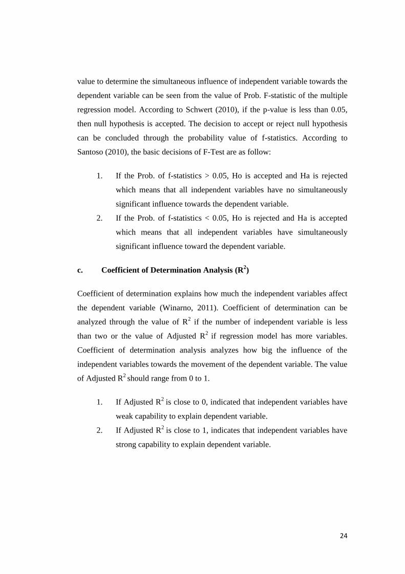
Table 4.1. Descriptive Statistic Result
Source: Processed secondary data
Descriptive statistic provides basic information of the object being researched in
this research, contains the summary of data such as the value of minimum,
maximum, mean, and standard deviation of each variable. Based on the output
above, it shows that:
a. The value of Mean
i. GDP : 3.08E+11
ii. FDI : 5.00E+09
iii. Export : 0.282
iv. Inflation : 0.097

26
b. The value of Standard Deviation
i. GDP : 2.86E+11
ii. FDI : 7.84E+09
iii. Export : 0.064
iv. Inflation : 0.091
c. The value of data processed is 35.
Based on the descriptive analysis result above, it shows the value of mean and
standard deviation of GDP is 3.08E+11 and 2.86E+11 respectively. It can be
estimated that approximately 95% of the values will fall in the range of 3.08E+11
– (1*2.86E+11) to 3.08E+11 + (1*2.86E+11) or between 2.2E+10 and 5.94E+11.
The value of mean is calculated from 1981 to 2015. Meanwhile, standard
deviation value is used to determine how wide the data will spread from minimum
value to the maximum value. Based on the mean and standard deviation, can be
concluded that the spread for GDP is 2.2E+10 to 5.94E+10 means that during the
period of 1981 until 2015, Indonesia maintained the GDP from 2.2E+10 point to
5.94E+11 point.
4.1.2. Normality of the Data
Figure 4.1. Normality Test of the Data
Source: Processed secondary data
27
This normality test is done with Ms. Excel as the tool to determine the normal
distribution of the data. From the figure above, it can be seen that with the total
data of 35, the data can be said normally distributed.
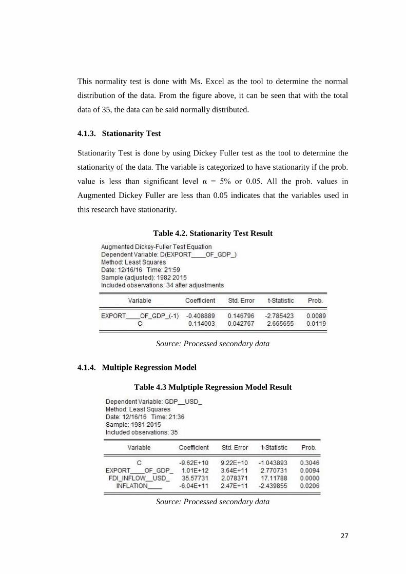
4.1.3. Stationarity Test
Stationarity Test is done by using Dickey Fuller test as the tool to determine the
stationarity of the data. The variable is categorized to have stationarity if the prob.
value is less than significant level α = 5% or 0.05. All the prob. values in
Augmented Dickey Fuller are less than 0.05 indicates that the variables used in
this research have stationarity.
Table 4.2. Stationarity Test Result
Source: Processed secondary data
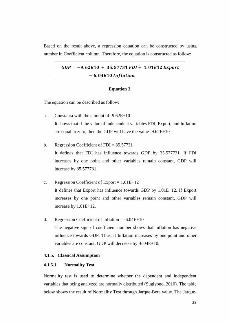
4.1.4. Multiple Regression Model
Table 4.3 Mulptiple Regression Model Result
Source: Processed secondary data
28
Based on the result above, a regression equation can be constructed by using
number in Coefficient column. Therefore, the equation is constructed as follow:
𝑮𝑫𝑷 = −𝟗.𝟔𝟐𝑬𝟏𝟎 + 𝟑𝟓.𝟓𝟕𝟕𝟑𝟏 𝑭𝑫𝑰 + 𝟏.𝟎𝟏𝑬𝟏𝟐 𝑬𝒙𝒑𝒐𝒓𝒕
− 𝟔.𝟎𝟒𝑬𝟏𝟎 𝑰𝒏𝒇𝒍𝒂𝒕𝒊𝒐𝒏
Equation 3.
The equation can be described as follow:
a. Constanta with the amount of -9.62E+10
It shows that if the value of independent variables FDI, Export, and Inflation
are equal to zero, then the GDP will have the value -9.62E+10
b. Regression Coefficient of FDI = 35.57731
It defines that FDI has influence towards GDP by 35.577731. If FDI
increases by one point and other variables remain constant, GDP will
increase by 35.577731.
c. Regression Coefficient of Export = 1.01E+12
It defines that Export has influence towards GDP by 1.01E+12. If Export
increases by one point and other variables remain constant, GDP will
increase by 1.01E+12.
d. Regression Coefficient of Inflation = -6.04E+10
The negative sign of coefficient number shows that Inflation has negative
influence towards GDP. Thus, if Inflation increases by one point and other
variables are constant, GDP will decrease by -6.04E+10.
4.1.5. Classical Assumption
4.1.5.1. Normality Test
Normality test is used to determine whether the dependent and independent
variables that being analyzed are normally distributed (Sugiyono, 2010). The table
below shows the result of Normality Test through Jarque-Bera value. The Jarque-

29
Bera value will be compared with X2
table with two degrees of freedom under
significant level α = 5%, which is 5.991. Based on the table below, the value of
Jarque-Bera is less than X2
which is 2.478781 < 5.991 and the prob. value is
greater than 0.05 which is 0.289581 > 0.05. As of the result, it can be concluded
that the data have normal distribution.
Table 4.4 Normality Test Result
Source: Processed secondary data
4.1.5.2. Heteroscedsticity Test
Table 4.5. Heteroscedasticity Test: Glejser Result
Source: Processed secondary data
Heteroscedasticity test aims to test whether there is disproportion variance of
residuals of one variable to another in regression model. If there is no
heteroscedasticity or there is homoscedasticity, then the regression model is

30
accepted. Heteroscedasticiy test can be seen from the value of Prob. F-statistic.
The table above shows the probability value is greater than the significant level.
Can be concluded that there are heteroscedasticity exists in the model.
4.1.5.3. Multicollinearity Test
Multicollinearity test is done to find out any correlation between one independent
variable and other independent variables in this research. According to Santoso
(2013), multicollinearity issue exists when there is any correlation. A good
regression model should not have correlation between the independent variables.
Table 4.6 Multicollinearity Test Result
Source: Processed secondary data
To know whether the multicollinearity exists between each independent variable,
it can be seen from the value of Centered Variance Inflation Factors (VIF) of each
variable. The value of Centered VIF should be in the range of 0.1 to 10. Based on
the table above, all values of Centered VIF of each variable are in the range of 0.1
to 10 where the value of FDI‟s Centered VIF is 1.142392, Export‟s Centered VIF
is 2.326990, and Inflation‟s Centered VIF is 2.163947. It means that there is no
multicollinearity between independent variables of the model.
4.1.5.4. Autocorrelation Test
Autocorrelation test is used to analyze whether there is a correlation of error
between t-period and t-1 period in the model. A good regression model is a model

31
without autocorrelation exists. To determine the autocorrelation status, it can be
seen from Durbin-Watson value. The value should be between -2 and 2 to indicate
the model has no autocorrelation.
Table 4.7. Durbin-Watson Test Result
Weighted Statistics
Durbin-Watson stat 1.531826
Source: Processed secondary data
Based on the table above, the result of Durbin-Watson test shows that the
regression model has no tendency of autocorrelation issue since the value is
1.531826 which is still in the range of -2 to 2. It means that the model has no
autocorrelation.
4.2. Hypothesis Testing
4.2.1. T-Test
T-test is used to know whether there is any significant influence between
independent variables toward dependent variable partially. To determine that the
independent variables have influence toward dependent variable, the value of
Prob. t-statistic should be less than significant level α = 5%. Based on Table 4.3.,
all of three independent variables which are FDI, Export, and Inflation have
partial significant influences toward GDP. The Prob. value of FDI, Export, and
Inflation are 0.0000, 0.0094, and 0.0206, respectively. The Prob. values are less
than significant level α = 5% indicates there is significant influence of each
variable towards dependent variable. The hypotheses of partial test are as follow:
H1: There is a significant influence between FDI towards GDP of Indonesia
H2: There is a significant influence between Export towards GDP of
Indonesia

32
H3: There is a significant influence between Inflation towards GDP of
Indonesia
As a result, H1, H2, and H3 are accepted since each independent variable (FDI,
Export, and Inflation) has significant influence towards dependent variable (GDP
of Indonesia).
4.2.2. F-Test
F-Test is conducted to determine the influence of independent variables
simultaneously toward dependent variable of this research. It can be determined
through the value of Prob. F-statistic result based on the calculation model, where
the value of Prob. F-statistic should be less than the significant level α = 5%. The
result is as follow:
Table 4.8. F-Test Result
Weighted Statistics
F-statistic
Prob(F-Statistic)
106.8092
0.000000
Source: Processeed secondary data
The hypothesis of overall significant test is as follow:
H4: There is a simultaneously significant influence between FDI, Export, and
Inflation towards GDP of Indonesia
Based on the table above, the value of Prob F-statistic is 0.000000 less than
significant level of α = 0.05 indicates there is a significant influence. Hence, H4 is
accepted since there is a simultaneous significant influence of FDI, Export, and
Inflation toward GDP of Indonesia.
4.2.3. Coefficient of Determination Analysis (R2)
Coefficient of determination (R2) defines how much the proportion of the
independent variables affect dependent variables (Winarno, 2011). This research
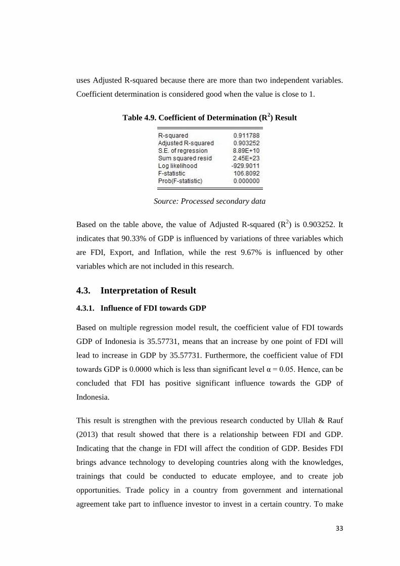
33
uses Adjusted R-squared because there are more than two independent variables.
Coefficient determination is considered good when the value is close to 1.
Table 4.9. Coefficient of Determination (R2) Result
Source: Processed secondary data
Based on the table above, the value of Adjusted R-squared (R2) is 0.903252. It
indicates that 90.33% of GDP is influenced by variations of three variables which
are FDI, Export, and Inflation, while the rest 9.67% is influenced by other
variables which are not included in this research.
4.3. Interpretation of Result
4.3.1. Influence of FDI towards GDP
Based on multiple regression model result, the coefficient value of FDI towards
GDP of Indonesia is 35.57731, means that an increase by one point of FDI will
lead to increase in GDP by 35.57731. Furthermore, the coefficient value of FDI
towards GDP is 0.0000 which is less than significant level α = 0.05. Hence, can be
concluded that FDI has positive significant influence towards the GDP of
Indonesia.
This result is strengthen with the previous research conducted by Ullah & Rauf
(2013) that result showed that there is a relationship between FDI and GDP.
Indicating that the change in FDI will affect the condition of GDP. Besides FDI
brings advance technology to developing countries along with the knowledges,
trainings that could be conducted to educate employee, and to create job
opportunities. Trade policy in a country from government and international
agreement take part to influence investor to invest in a certain country. To make

34
Indonesia more interesting to invest, government may create more friendly
investment policies and improve infrastructure which is currently being worked
on.
4.3.2. Influence of Export towards GDP
Multiple regression model result shows the coefficient value of Export towards
GDP of Indonesia which is 1.01E+12. It means that every increase of Export by
one point will lead to increase of GDP by 1.01E+12. Moreover, the prob.value of
Export towards GDP is less than 0.05 which is 0.009. Thus, Export is found to be
significant and have positive influence towards GDP. It indicates the change of
Export will affect the level of GDP of Indonesia.
This result is in line with the results from previous research that conducted by
Ullah & Rauf (2013) that Export has significant influence towards GDP. Export is
part of national income besides can bring welfare through employment for the
people. If the value of Export exceeds the value of Import, it will increase the
value of GDP. However, according to World Bank (2016) the value of Net Export
of Indonesia is falling steadily with greater amount of Import than Export in the
past few years, affecting the value of GDP. On the other hand, researcher found
that if a country‟s national income depends too much on Export, a country could
be vulnerable to world economic condition.
4.3.3. Influence of Inflation towards GDP
Coefficient value of Inflation towards GDP as shows in multiple regression model
is -6.04E+11. Meaning to say that every increase of Inflation by one point will
lead to increase of GDP by -6.04E+11. Therefore, can be concluded that Inflation
has negative significant influence towards GDP of Indonesia and the third
hypothesis that states there is a significant influence of Inflation on GDP is
accepted.
Unstable political condition affecting the rapid increase of price in the market or
inflation and it influence the investment. Therefore, the well-maintained and
35
stable inflation will have price stability to ensure people to invest. The findings is
in accordance with result from a research conducted by Davcev & Hourvouliades
(2015) that Inflation has influence on GDP of Romania and Bulgaria.
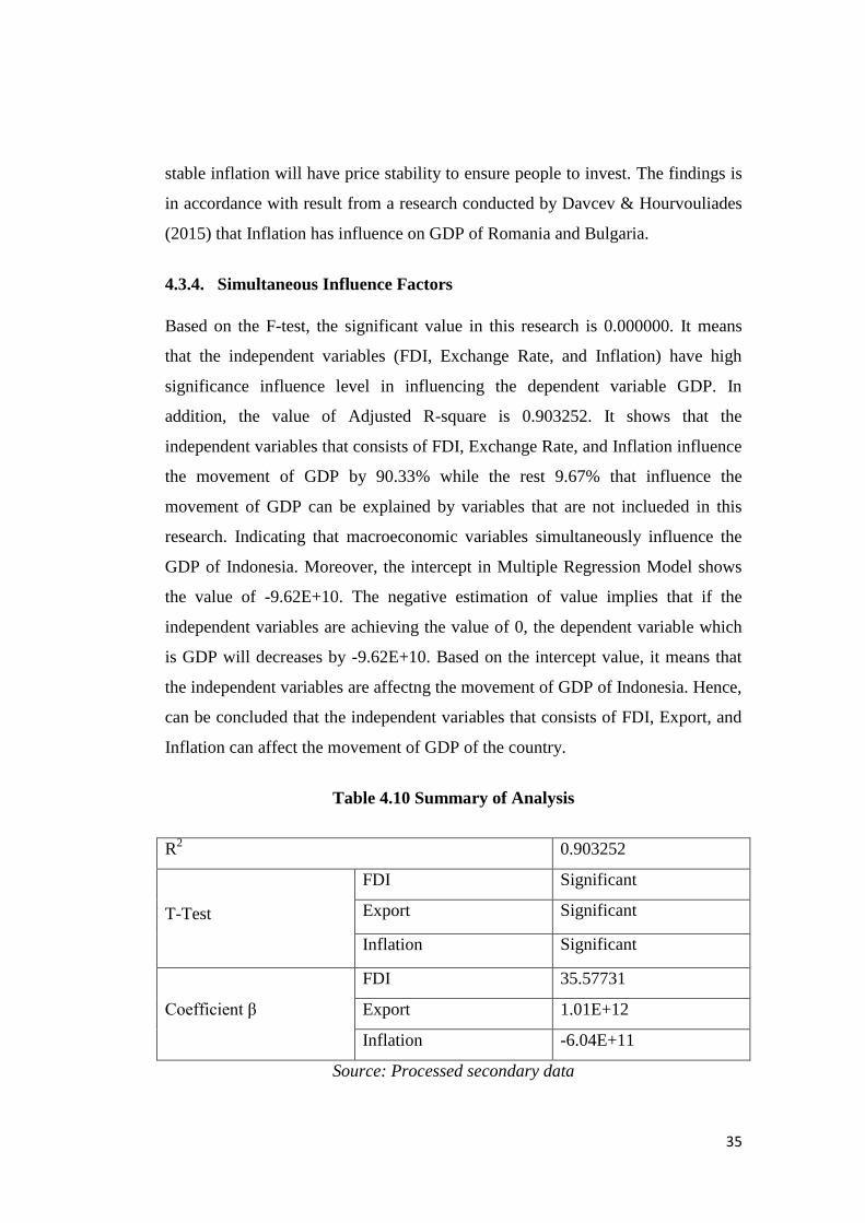
4.3.4. Simultaneous Influence Factors
Based on the F-test, the significant value in this research is 0.000000. It means
that the independent variables (FDI, Exchange Rate, and Inflation) have high
significance influence level in influencing the dependent variable GDP. In
addition, the value of Adjusted R-square is 0.903252. It shows that the
independent variables that consists of FDI, Exchange Rate, and Inflation influence
the movement of GDP by 90.33% while the rest 9.67% that influence the
movement of GDP can be explained by variables that are not inclueded in this
research. Indicating that macroeconomic variables simultaneously influence the
GDP of Indonesia. Moreover, the intercept in Multiple Regression Model shows
the value of -9.62E+10. The negative estimation of value implies that if the
independent variables are achieving the value of 0, the dependent variable which
is GDP will decreases by -9.62E+10. Based on the intercept value, it means that
the independent variables are affectng the movement of GDP of Indonesia. Hence,
can be concluded that the independent variables that consists of FDI, Export, and
Inflation can affect the movement of GDP of the country.
Table 4.10 Summary of Analysis
R2 0.903252
T-Test
FDI Significant
Export Significant
Inflation Significant
Coefficient β
FDI 35.57731
Export 1.01E+12
Inflation -6.04E+11
Source: Processed secondary data
36
CHAPTER V
CONCLUSION AND RECOMMENDATION
This chapter defines the conclusions according to the stated scope and limitation
and recommendation for related parties which are government of Indonesia and
future researcher as stated in the significance of the study.
5.1. Conclusion
The objective of this research is to analyze the influence of macroeconomic
factors toward GDP of Indonesia during the year period 1981 – 2015 in annual
basis. This research is conducted wth purposive sampling and time series data
method with a total of 35 observations. This research uses descriptive analysis,
classical assumption test, and hypothesis testing for the analysis. Thus, based on
the analysis which have been done, there are several conclusions that can be
drawn as follow:
From t-test result, the significant influence of each independent variable is
desrcribed as follow:
a. FDI has positive significant influence towards GDP of Indonesia.
H1: There is a significant influence between FDI towards GDP of
Indonesia
Based on the findings, H1 is accepted. The more FDI a country receive,
the more the value of GDP. By keep the stable inflation, keep
improving the infrastructure, have a friendly agreement and clear policy
to make the country interesting to invest.
b. Export has positive significant influence towards GDP of Indonesia.
H2: There is a significant influence between Export towards GDP of
Indonesia

37
Based on the result, H2 is accepted. The more the export of a country
the more it will bring job opportunities and support the country‟s
economic, and to build and maintain relationship with other countries.
Export is influenced by exchange rate, when the money value is high it
may decrease the number of Export.
c. Inflation has negative significant influence towards GDP of Indonesia.
H3: There is a significant influence between Inflation towards GDP of
Indonesia
According to the result, H3 is accepted. The change of Inflation rate
will influence the price stability that will influence to consumption level
of people, government expenditure, number of export, and investment.
Unstable and high inflation will affect the price stability and when
people can‟t afford the same amount of goods with the same number of
money, because the value of the money decreases.
5.1.2. From F-Test result, all independent variables which are FDI, Export, and
Inflation are concluded to have significant influence toward GDP of
Indonesia. The significant value of the F-Test is 0.000000, it means that all
independent varables have a high significant level in influencing the GDP
of Indonesia. FDI, Export, and Inflation are influencing the GDP by
90.33% while the remaining 9.67% is influenced by other variables
outside of this research. Indicating that the dependent variable which is
GDP is sensitive of the change in macroeconomic variables
simultaneously.
5.2. Future Recommendation
5.2.1. For Government
Researcher suggests the Government of Indonesia to have the Inflation rate well
maintained at low and stable for as long as possible in order to have price
stability. Price stability will ensure people to invest because the value of money

38
will be stable over time. Besides that, firms and consumers put investment
decision on information from prices. Unstable price level will complicate the
forecast of real return of investment project. In addition to Inflation rate,
researcher suggests the government to focus on Net Export or value of exports
minus imports. When the value of exports exceeds import, the Net Export will be
positive, the positive Net Exports will contribute to the national income, besides it
means more output from the domestic industries, ran by greater number of
employee. It will contribute to economic growth and reduces the number of
unemployment. Moreover, government may try to control the political conditions,
as political condition play a crucial part in the country. Political conditions
impacted the safety and economy of a country directly.
5.2.2. For Future Researcher
For future researcher, the researcher initiates to offer several recommendation and
suggestion for the future research related to the influence of macroeconomic
factors towards GDP. There are several variables that unfortunately are unable to
be used in this research which are labor force, import, savings, tax revenue,
consumer price index, and public debt. In addition, future researcher can analyze
the data monthly if there is supported data in order to gain more accuracy of
research. In addition, future researcher may widen the scope and limitation like
the time period or other samples. The last but not least, researcher suggests future
researcher who interested in economic may be able to examine the influence of
economic growth towards poverty, as it is known that poverty is still a concern for
developing countries.
39
REFERENCES
Books
Cooper, Donald R & Schindler, Pamela S., (author.) (2014). Business research
methods (Twelfth Edition, Mc Graw Hill International Edition). New
York, N.Y. McGraw-Hill
DeLong, J. B., & Olney, M. L. (2006). Macroeconomics (2nd ed., 0-07-111113-
1). New York, America: McGraw-Hill/Irwin.
Gujarati, D. N. (2004). Basic Econometrics. McGraw-Hill
Hahn, F. H. (2010). Economic Growth (978-0-230-28082-3) (S. N. Durlauf & L.
E. Blume, Eds.). United Kingdom: Palgrave Macmillan UK.
Karya, D., & Syamsuddin, S. (2016). Makro Ekonomi; Pengantar untuk
Manajemen ( 978-979-769-953-6). Jakarta: Rajawali Press.
Moosa, I. A. (2002). Foreign Direct Investment Theory, Evidence and Practice.
New York: PALGRAVE.
Rosadi, D. (2012). Ekonometrika & Analisis Runtun Waktu Terapan Dengan
Eviews. Yogyakarta: Penerbit Andi Yogyakarta
Santoso, S. (2013). Menguasai SPSS 21 di Era Informasi. Jakarta: PT Elex Media.
Seyoum, B. (2014). Export Import Theory, Practices, and Procedure (3rd ed.,
Ser. 9780203581506). New York: Routledge.
Sugiyono. (2010). Metode Penelitian Kuantitatif Kualitatif & RND. Bandung:
Alfabeta.
Weiss, N. A. (2012). Introductory Statistics. USA: Addison-Wesley
Winarno, Wing Wahyu (2011). Analisis Ekonometrika dan Statistika dengan
EViews. Yogyakarta: Unit Penerbit dan Percetakan STIM YKPN
Yogyakarta.
Journals
Abdu, M. (2013). Foreign Direct Investment And Economic Growth In Nigeria.
Conference of the International Journal of Arts & Sciences, 1942-6114,
63-72.
Davcev, L., & Hourvouliades, N. (2015). Impact of Interest Rate and Inflation on
GDP in Bulgaria, Romania and Fyrom. The Eleventh International

40
Conference:“Challenges of Europe: Growth, competitiveness and
inequality”, 19-38.
Elia, S., Maggi, E., & Mariotti, I. (2013). Horizontal, Vertical and Conglomerate
Investments in the Italian Logistics Industry: Drivers and Strategies.
Enu, E. D. (2013, July). Macroeconomic Determinants Of Economic Growth In
Ghana: Cointegration Approach. European Scientific Journal, 9, 1857-
7431, 156-175
Ghozali, I. (2005). Aplikasi Analisis Multivariate dengan Program SPSS.
Semarang: BP UNDIP.
Herger, N., & McCorriston, S. (2013, February). Horizontal, Vertical, and
Conglomerate FDI: Evidence from Cross Border Acquisitions. 1-23.
Kryeziu, A. (2016, March). The Impact Of Macroeconomic Factors In Economic
Growth. European Scientific Journal, 12(7), 1857-7431, 331-345.
Muchlas, Z., & Alamsyah, A. R. (n.d.). Faktor-faktor Yang Mempengaruhi Kurs
Rupiah Terhadap Dolar Amerika Pasca Krisis (2000-2010). Jurnal
JIBEKA, 9(1), 76-86
Olusanya, S. O. (2013, September). Impact Of Foreign Direct Investment Inflow
On Economic Growth In A Pre and Post Deregulated Nigeria Economy. A
Granger Casuality Test (1970-2010). European Scientific Journal, 9,
1857- 7431, 335-356.
.
Ullah, F., & Rauf, A. (2013). Impacts of Macroeconomic Variables On Economic
Growth: A Panel Data Analysis Of Selected Asian Countries. International
Journal of Information, Business and Management, 5(2), 2076-9202, 4-12.
Yin, J., & Tian, L. (2013). The Impact Of Foreign Direct Investment On
Economic Growth In China. Advances and Applications in Statistics, 36,
75-81.
Electronic Sources
Badan Pusat Statistik. (2016). Retrieved October 28, 2016, from
https://www.bps.go.id/
Bank Indonesia. (2016). Retrieved October 27, 2016, from http://www.bi.go.id/
Begley, S. (2016, January 20). This Is the Best Country in the World. Retrieved
October 10, 2016, from http://time.com/4186601/best-country-in-the-
world-davos/
41
Indonesia Population (LIVE). (2016). Retrieved October 10, 2016, from
http://www.worldometers.info/world-population/indonesia-population/
Inflation Indonesia 1998. (2016). Retrieved November 11, 2016, from
http://www.inflation.eu/inflation-rates/indonesia/historic-inflation/cpi-
inflation-indonesia-1998.aspx
Meko, D. (2013). Applied Time Series Analysis. Retrieved December 19, 2016,
from Laboratory of Tree-Ring :
http://www.ltrr.arizona.edu/~dmeko/geos585a.html
Sawitri, A. A. (2016, April 1). BI: Lebih Baik Inflasi Dijaga di Bawah 4,5 Persen.
BI: Lebih Baik Inflasi Dijaga di Bawah 4,5 Persen. Retrieved from
https://m.tempo.co/read/news/2016/04/01/087758933/bi-lebih-baik-inflasi-
dijaga-di-bawah-4-5-persen
Sholeh, M., & Hasits, M. (2015, August 25). Jokowi beberkan alasan penyebab
ekonomi melemah dan rupiah loyo. Merdeka. Retrieved November 2,
2016, from https://www.merdeka.com/peristiwa/jokowi-beberkan-alasan-
penyebab-ekonomi-melemah-dan-rupiah-loyo.html.
Schwert, G. W. (2010, April 2). Descriptive Statistic & Test. Retrieved December
19, 2016, from EViews 7 User's Guide I:
http://schwert.ssb.rochester.edu/a425/EV71.pdf
Simpson, S. D. (2014). Macroeconomics: Inflation. Retrieved October 29, 2016.
Wiyanti, S. (2013, August 24). Ini perbedaan krisis ekonomi 1998, 2008 dan 2013
versi BI. Merdeka. Retrieved November 2, 2016, from
https://www.merdeka.com/uang/ini-perbedaan-krisis-ekonomi-1998-2008-
dan-2013-versi-bi.html.
World Bank (2016). Retrieved October 29, 2016, from http://data.worldbank.org/

42
APPENDICES
Appendix 1: Raw Data
Year GDP (USD) FDI (USD) Export (%) Inflation (%)
1981 92,474,000,000 133,000,000 29.040 12.244
1982 94,715,000,000 225,000,000 25.303 9.481
1983 85,369,000,000 292,000,000 26.343 11.787
1984 87,612,000,000 222,000,000 25.587 10.456
1985 87,339,000,000 310,000,000 22.201 4.729
1986 80,061,000,000 258,000,000 19.487 5.827
1987 75,930,000,000 385,000,000 23.934 9.275
1988 88,788,000,000 576,000,000 23.776 8.043
1989 101,455,000,000 682,000,000 24.287 6.418
1990 114,426,000,000 1,093,000,000 25.329 7.813
1991 128,168,000,000 1,482,000,000 25.797 9.416
1992 139,116,000,000 1,777,000,000 27.891 7.526
1993 158,007,000,000 2,004,000,000 26.755 9.688
1994 176,892,000,000 2,109,000,000 26.511 8.518
1995 202,132,000,000 4,346,000,000 26.312 9.432
1996 227,370,000,000 6,194,000,000 25.825 7.968
1997 215,749,000,000 4,677,000,000 27.859 6.230
1998 95,446,000,000 -240,800,000 52.968 58.387
1999 140,001,000,000 -1,866,000,000 35.514 20.489
2000 165,021,000,000 -4,550,000,000 40.977 3.720
2001 160,447,000,000 -2,977,000,000 39.032 11.502
2002 195,661,000,000 145,085,549 32.688 11.879
2003 234,772,000,000 -596,923,828 30.478 6.586

43
2004 256,837,000,000 1,896,000,000 32.217 6.244
2005 285,869,000,000 8,336,000,000 34.067 10.452
2006 364,571,000,000 4,914,000,000 31.035 13.109
2007 432,217,000,000 6,928,000,000 29.436 6.407
2008 510,229,000,000 9,318,000,000 29.808 9.777
2009 539,580,000,000 4,877,000,000 24.159 4.814
2010 755,094,000,000 15,292,000,000 24.299 5.133
2011 892,969,000,000 20,565,000,000 26.327 5.357
2012 917,870,000,000 21,201,000,000 24.594 4.280
2013 912,524,000,000 23,282,000,000 23.924 6.413
2014 890,487,000,000 26,277,000,000 23.634 6.395
2015 861,934,000,000 15,508,000,000 21.092 6.363

44

45

46
Top Related