


Languages
Pages
Legal

The Inefficient Stock MarketWhat Pays Off and Why
(Prentice Hall, 1999)Visit our web-site at HaugenSystems.com

What

Probability Distribution For Returns to a Portfolio
Possible Rates of Returns
Probability
Expected Return
Variance of Return
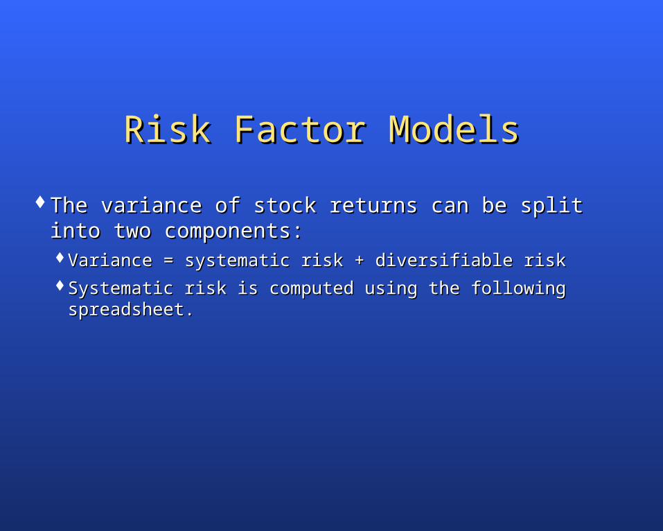
Risk Factor ModelsRisk Factor Models
The variance of stock returns can be split into two The variance of stock returns can be split into two components:components:Variance = systematic risk + diversifiable riskVariance = systematic risk + diversifiable riskSystematic risk is computed using the following spreadsheet.Systematic risk is computed using the following spreadsheet.

Risk Factor ModelsRisk Factor Models
Factor betas are estimated by relating stock returns Factor betas are estimated by relating stock returns to (unexpected) percentage changes in the factor to (unexpected) percentage changes in the factor over a period where the stock’s character is similar over a period where the stock’s character is similar to the present.to the present.

Relationship Between Return to General Relationship Between Return to General Electric and Changes in Interest Rates Electric and Changes in Interest Rates
-25%-25%
-20%-20%
-15%-15%
-10%-10%
-5%-5%
0%0%
5%5%
10%10%
15%15%
20%20%
25%25%
Return to G.E.Return to G.E.
-10%-10% -5%-5% 0%0% 5%5% 10%10%
Percentage Change in Yield on Long-term Govt. Bond Percentage Change in Yield on Long-term Govt. Bond
Line of Best FitLine of Best Fit
April, 1987April, 1987
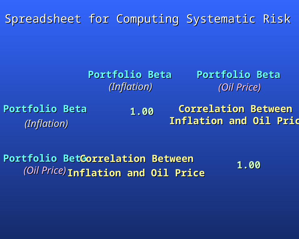
Spreadsheet for Computing Systematic RiskSpreadsheet for Computing Systematic Risk
Portfolio BetaPortfolio Beta Portfolio BetaPortfolio Beta(Inflation)(Inflation) (Oil Price)(Oil Price)
1.001.00 Correlation BetweenCorrelation BetweenInflation and Oil PriceInflation and Oil Price
Portfolio BetaPortfolio Beta
(Inflation)(Inflation)
Portfolio BetaPortfolio Beta(Oil Price)(Oil Price)
Correlation BetweenCorrelation Between
Inflation and Oil PriceInflation and Oil Price 1.001.00
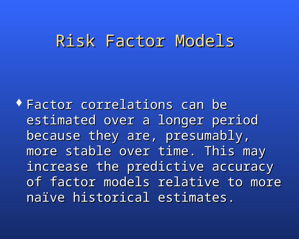
Risk Factor ModelsRisk Factor Models
Factor correlations can be estimated over a Factor correlations can be estimated over a longer period because they are, presumably, longer period because they are, presumably, more stable over time. This may increase the more stable over time. This may increase the predictive accuracy of factor models relative to predictive accuracy of factor models relative to more naïve historical estimates. more naïve historical estimates.
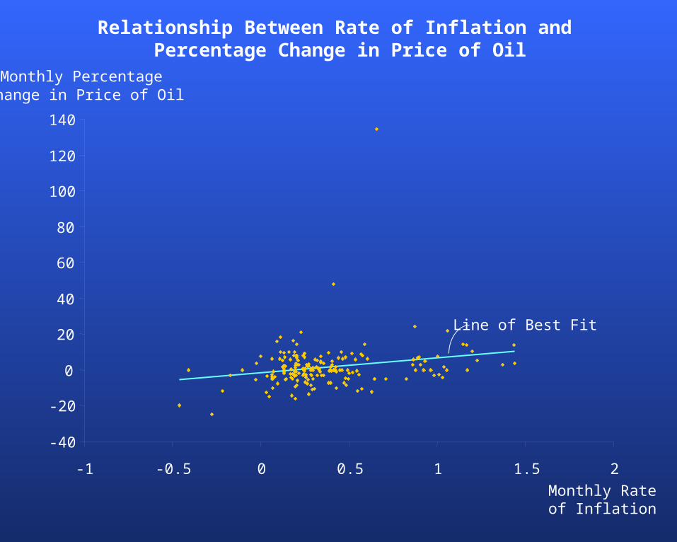
Relationship Between Rate of Inflation and Percentage Change in Price of Oil
-1 -0.5 0 0.5 1 1.5 2Monthly Rate of Inflation
-40
-20
0
20
40
60
80
100
120
140
Monthly Percentage Change in Price of Oil
Line of Best Fit

Computing Portfolio Systematic RiskComputing Portfolio Systematic Risk
Portfolio Beta * Portfolio Beta * 1.001.00
(Inflation) (Inflation)
+Portfolio Beta * Portfolio Beta * Correlation Between(Inflation) (Oil Price) Inflation and Oil Price
+Portfolio Beta * Portfolio Beta * 1.001.00 (Oil Price) (Oil Price)
+Portfolio Beta * Portfolio Beta * Correlation Between (Inflation) (Oil Price) Inflation and Oil Price
=Portfolio Systematic RiskPortfolio Systematic Risk

Risk Factor ModelsRisk Factor Models
If your factors have truly captured the structure behind the If your factors have truly captured the structure behind the correlations between stock returns, then portfolio diversifiable correlations between stock returns, then portfolio diversifiable risk can be estimated by summing the products of (a) the risk can be estimated by summing the products of (a) the diversifiable risk of each stock and (b) the square of its portfolio diversifiable risk of each stock and (b) the square of its portfolio weight.weight.
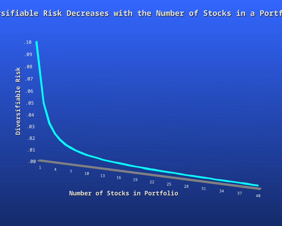
DiversifiableDiversifiable Risk Decreases with the Number of Stocks in a PortfolioRisk Decreases with the Number of Stocks in a Portfolio
40
1 47 10
13 1619
2225
2831
3437
.00
.01
.02
.03
.04
.05
.06
.07
.08
.09
.10
Div
ersi
fiab
le R
isk
D
iver
sifi
able
Ris
k
Number of Stocks in PortfolioNumber of Stocks in Portfolio

Study by Fedenia Study by Fedenia (University of Wisconsin)(University of Wisconsin)
Study covers all NYSE stocks (1963-94)Study covers all NYSE stocks (1963-94) Goal is to find lowest volatility portfolio for next 12 months for 100 randomly selected stks.Goal is to find lowest volatility portfolio for next 12 months for 100 randomly selected stks. The naïve estimate finds the low volatility portfolio over the previous 60 months.The naïve estimate finds the low volatility portfolio over the previous 60 months. Creates a risk model using, as factors, 5 portfolios that account for the correlations between Creates a risk model using, as factors, 5 portfolios that account for the correlations between
the 100 stocks.the 100 stocks. Finds the lowest volatility portfolio with risk model.Finds the lowest volatility portfolio with risk model. Repeats process 270 times for each year.Repeats process 270 times for each year.
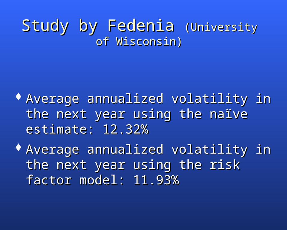
Study by Fedenia Study by Fedenia (University of Wisconsin)(University of Wisconsin)
Average annualized volatility in the next year Average annualized volatility in the next year using the naïve estimate: 12.32%using the naïve estimate: 12.32%
Average annualized volatility in the next year Average annualized volatility in the next year using the risk factor model: 11.93%using the risk factor model: 11.93%

Expected Return Factor ModelsExpected Return Factor Models The factors in an expected return model represent the character of the The factors in an expected return model represent the character of the
companies. They might include the history of their stock prices, its size, companies. They might include the history of their stock prices, its size, financial condition, cheapness or dearness of prices in the market, etc.financial condition, cheapness or dearness of prices in the market, etc.
Factor payoffs are estimated by relating individual stock returns to Factor payoffs are estimated by relating individual stock returns to individual stock characteristics over the cross-section of a stock individual stock characteristics over the cross-section of a stock population (here the largest 3000 U.S. stocks).population (here the largest 3000 U.S. stocks).

Five Factor FamiliesFive Factor Families
Risk Risk LiquidityLiquidityPrice level Price level Growth potentialGrowth potentialPrice historyPrice history
-1.0 -0.5 0.0 0.5 1.0 1.5 2.0 2.5 3.0
Book to Price
-100%
-50%
0%
50%
100%
-1.5
Tota
l R
etu
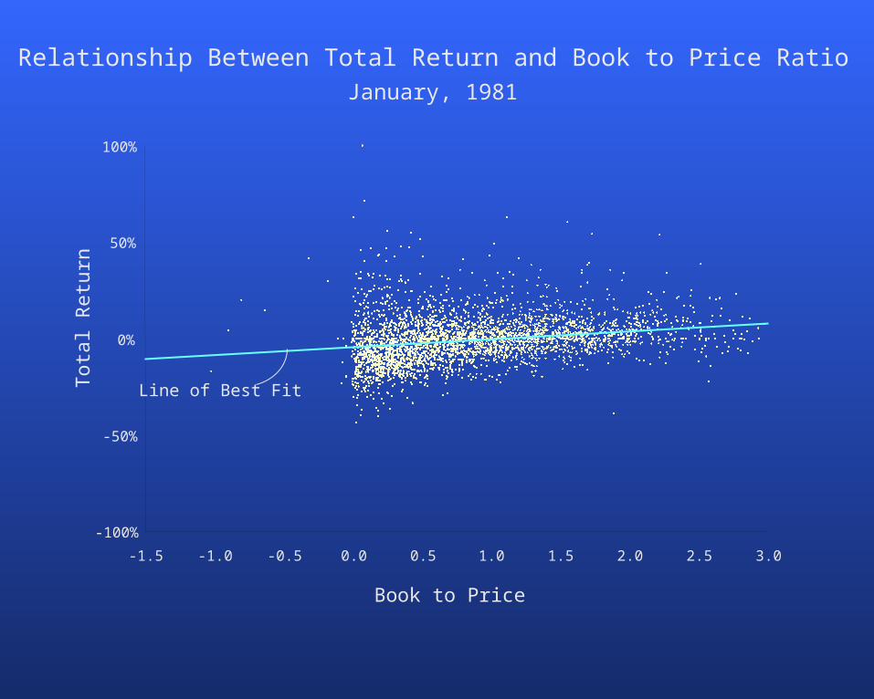
rnRelationship Between Total Return and Book to Price Ratio
January, 1981
Line of Best Fit
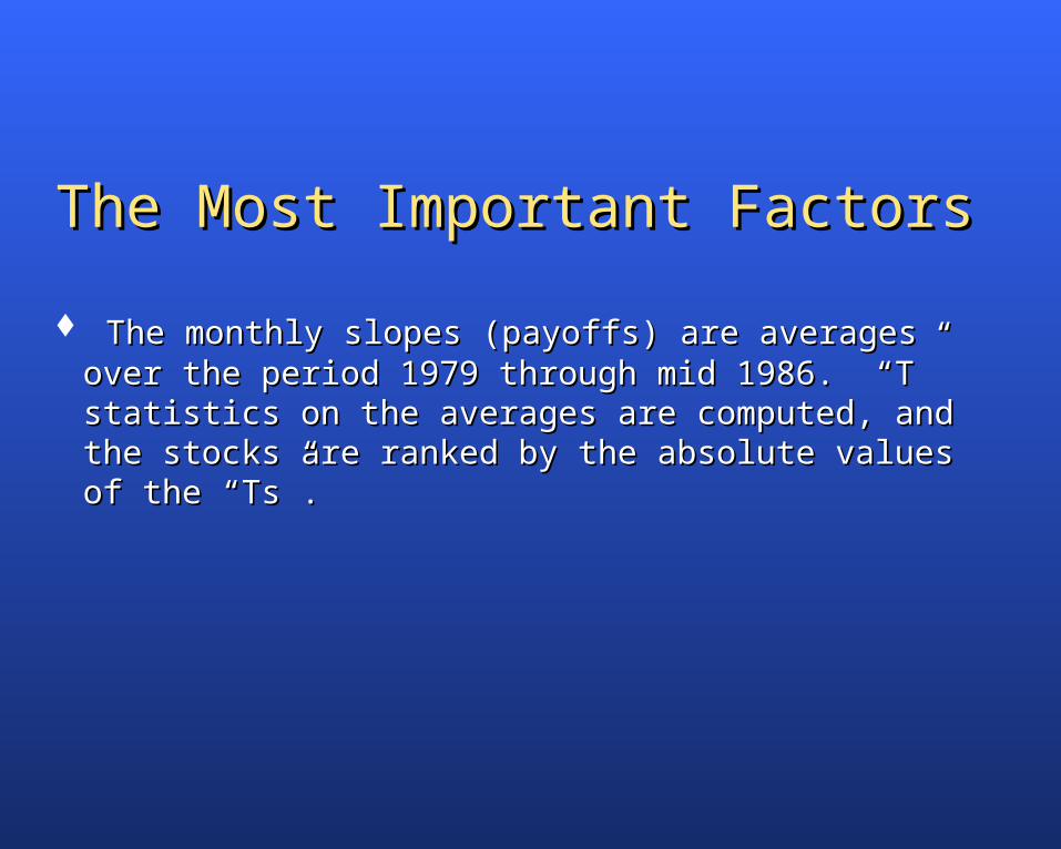
The Most Important FactorsThe Most Important Factors
The monthly slopes (payoffs) are averages over the The monthly slopes (payoffs) are averages over the period 1979 through mid 1986. “T” statistics on the period 1979 through mid 1986. “T” statistics on the averages are computed, and the stocks are ranked by averages are computed, and the stocks are ranked by the absolute values of the “Ts”.the absolute values of the “Ts”.

Most Important Factors
1979/01 through1986/06
1986/07 through 1993/12
Factor Mean Confidence Mean Confidence
One-month excess return -0.97% 99% -0.72% 99%
returnTwelve-month excess 0.52% 99% 0.52% 99%
Trading volume/marketcap
-0.35% 99% -0.20% 98%
Two-month excess return -0.20% 99% -0.11% 99%
Earnings to price 0.27% 99% 0.26% 99%
Return on equity 0.24% 99% 0.13% 97%
Book to price 0.35% 99% 0.39% 99%
Trading volume trend -0.10% 99% -0.09% 99%
Six-month excess return 0.24% 99% 0.19% 99%
Cash flow to price 0.13% 99% 0.26% 99%

Projecting Expected ReturnProjecting Expected Return
The components of expected return are obtained by multiplying the projected The components of expected return are obtained by multiplying the projected payoffpayoff to each factor (here the average of the past 12) by the stock’s current to each factor (here the average of the past 12) by the stock’s current exposureexposure to the to the factor. Exposures are measured in standard deviations from the cross-sectional mean.factor. Exposures are measured in standard deviations from the cross-sectional mean.
The individual components are then summed to obtain the aggregate expected return The individual components are then summed to obtain the aggregate expected return for the next period (here a month)for the next period (here a month)
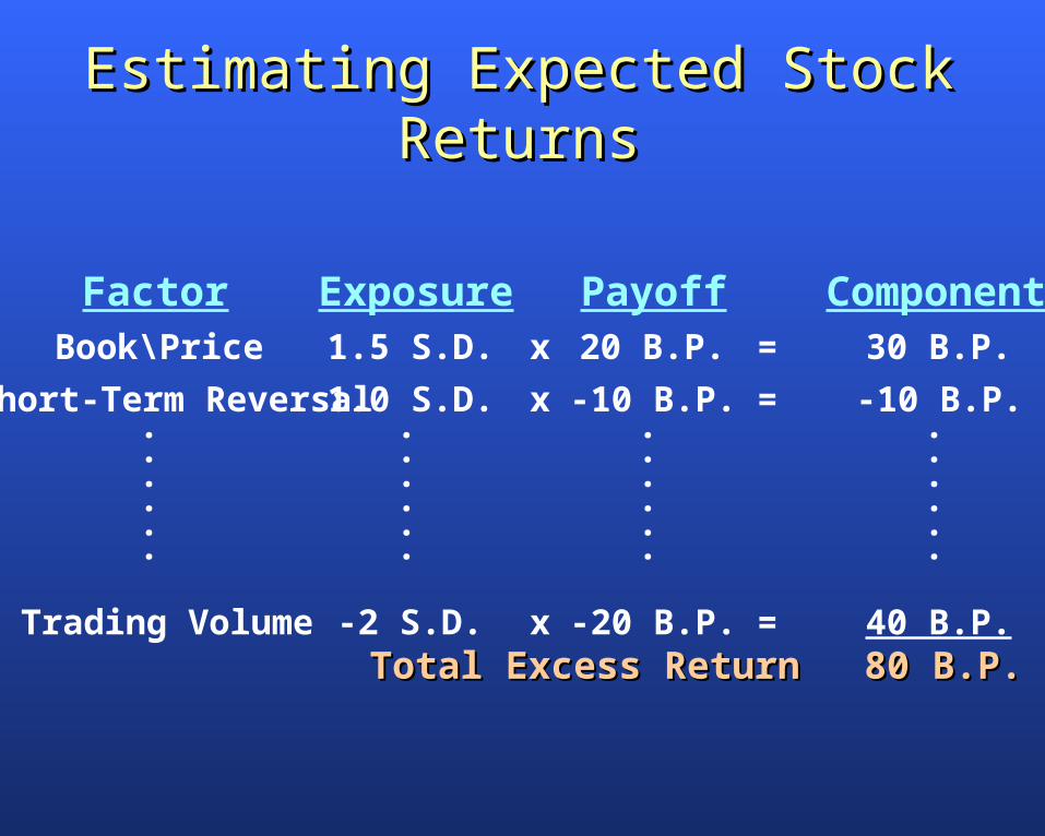
Factor Exposure Payoff ComponentBook\Price 1.5 S.D. x 20 B.P. = 30 B.P.
Short-Term Reversal 1.0 S.D. x -10 B.P. = -10 B.P.. . . .. . . .. . . .. . . .. . . .. . . .
Estimating Expected Stock ReturnsEstimating Expected Stock Returns
Trading Volume -2 S.D. x -20 B.P. = 40 B.P.Total Excess ReturnTotal Excess Return 80 B.P.80 B.P.

The Model’s Out-of-sample Predictive The Model’s Out-of-sample Predictive PowerPower
The 3000 stocks are ranked by expected return and formed into deciles The 3000 stocks are ranked by expected return and formed into deciles (decile 10 highest).(decile 10 highest).
The performance of the deciles is observed in the next month. Then The performance of the deciles is observed in the next month. Then expected returns are re-estimated, and the deciles are re-ranked.expected returns are re-estimated, and the deciles are re-ranked.
The process continues through 1993.The process continues through 1993.
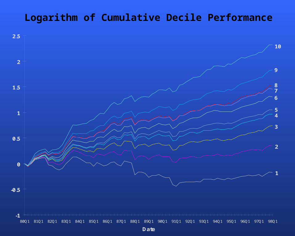
Logarithm of Cumulative Decile Performance
1
2
3
45
678
9
10
-1
-0.5
0
0.5
1
1.5
2
2.5
80Q1 81Q1 82Q1 83Q1 84Q1 85Q1 86Q1 87Q1 88Q1 89Q1 90Q1 91Q1 92Q1 93Q1 94Q1 95Q1 96Q1 97Q1 98Q1
Date

3 4 5 6 7 8 9 10Decile
-40%
-30%
-20%
-10%
0%
10%
20%
30%
0 1 2
Realized Return
Realized Return for 1984 by Decile
(Y/X = 5.5%)
Y
X

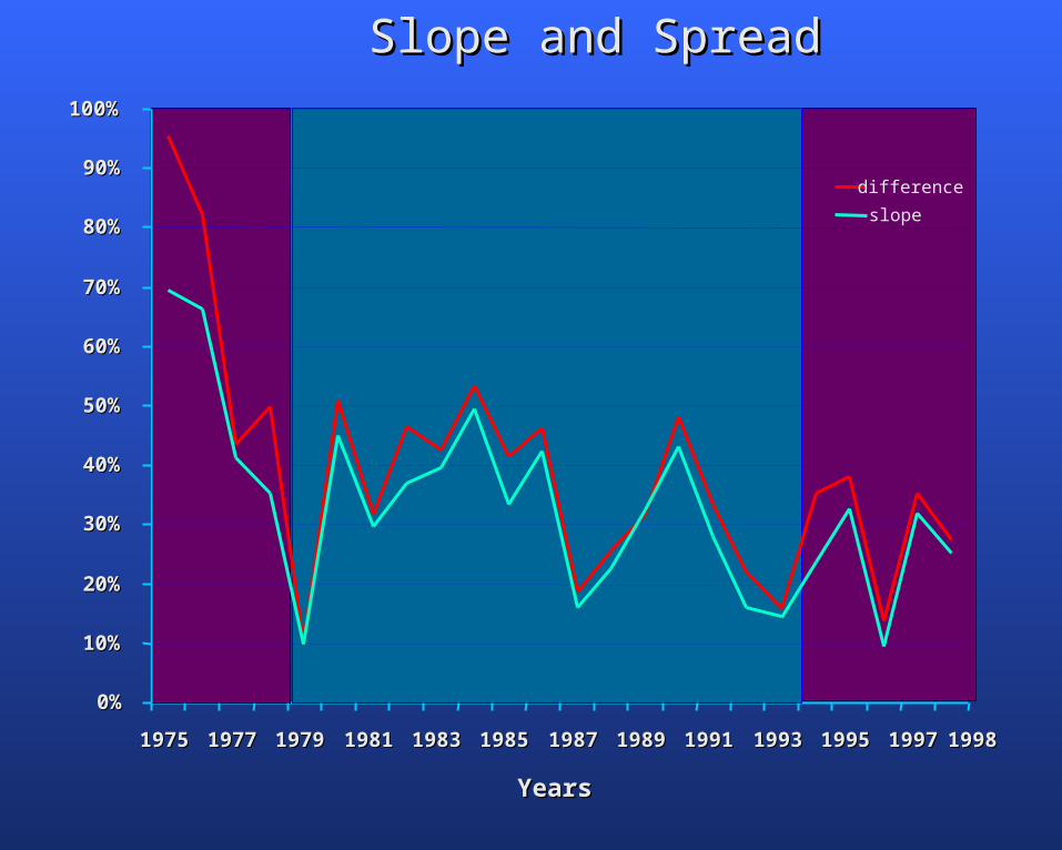
Extension of Study to Other Periods
(Nardin Baker)
• The same family of factors is used on a similar stock population.
• Years before and after initial study period are examined to determine slopes and spreads between decile 1 and 10.
19971997
0%0%
10%10%
20%20%
30%30%
40%40%
50%50%
60%60%
70%70%
80%80%
90%90%
100%100%
19751975 19771977 19791979 19811981 19831983 19851985 19871987 19891989 19911991 19931993 19951995
YearsYears
19981998
difference
slope
Slope and SpreadSlope and Spread

Decile Risk Characteristics
The characteristics reflect the character of the deciles over the period 1979-1993.

Fama-French Three- Factor Model
Monthly decile returns are regressed on monthly differences in the returns to the following:
S&P 500 and T bills.
The 30% of stocks that are smallest and largest.
The 30% of stocks with highest book-to-price and the lowest.

Sensitivities (Betas) to Market Returns
10
Decile
1 2 3 4 5 6 7 8 9
0.95
1
1.05
1.1
1.15
1.2
1.25
Market Beta
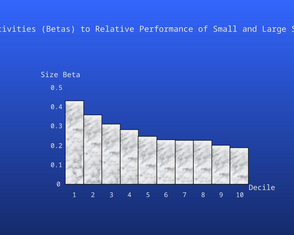
Sensitivities (Betas) to Relative Performance of Small and Large Stocks
2 3 4 5 6 7 8 9 10Decile0
0.1
0.2
0.3
0.4
0.5
1
Size Beta
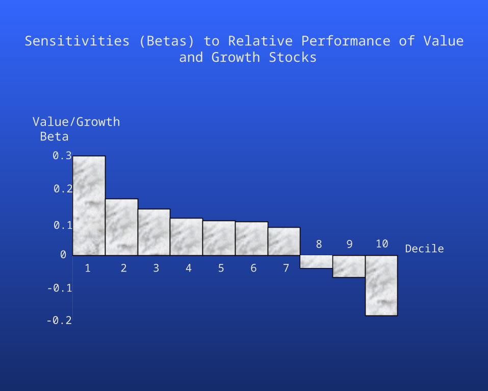
Sensitivities (Betas) to Relative Performance of Value and Growth Stocks
Decile8 9 10
1 2 3 4 5 6 7
-0.2
-0.1
0
0.1
0.2
0.3
Value/Growth Beta
Fundamental Characteristics
Averaged over all stocks in each decile and over all months (1979-83)

Risk
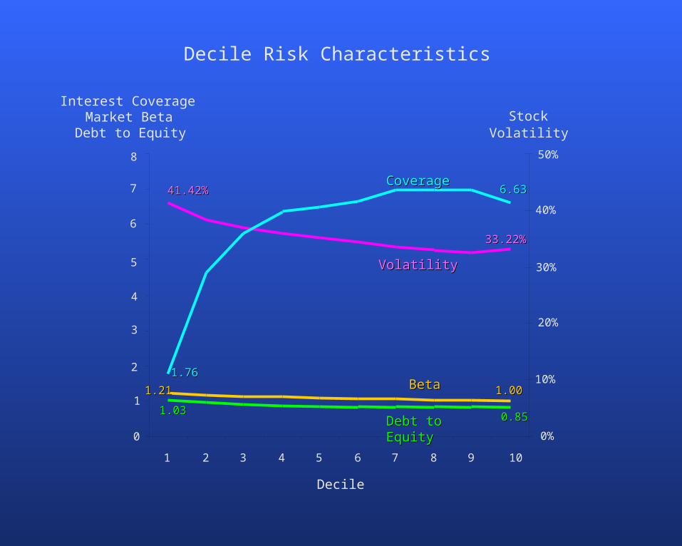
Decile Risk Characteristics
Debt to EquityDebt to Equity
1.031.030.850.85
StockVolatility
1 2 3 4 5 6 7 8 9 10
Decile
0%0
1
2
3
4
5
6
7
8
Interest CoverageMarket Beta
Debt to Equity
VolatilityVolatility
41.42%41.42%
33.22%33.22%
10%
20%
30%
40%
50%
Coverage Coverage
1.761.76
6.636.63
BetaBeta 1.001.001.211.21

Liquidity
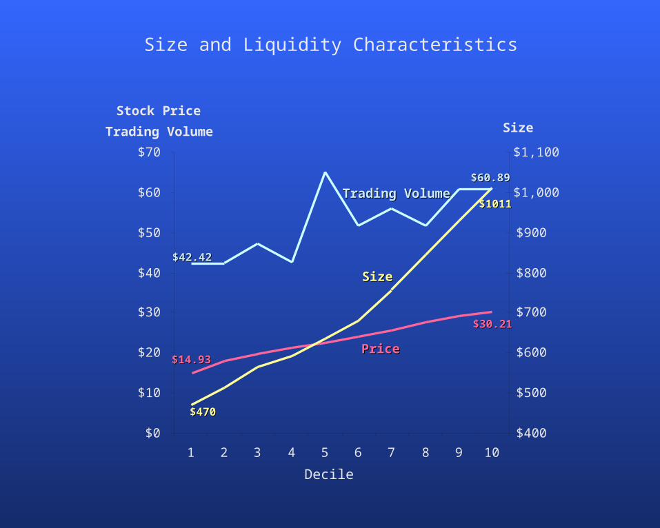
Size and Liquidity Characteristics
$0
$10
$20
$30
$40
$50
$60
$70
1 2 3 4 5 6 7 8 9 10
Decile
Stock Price
Trading Volume
$400
$500
$600
$700
$800
$900
$1,000
$1,100
Size
$14.93$14.93
$30.21$30.21
PricePrice
$470$470
$1011$1011
SizeSize
$42.42$42.42
$60.89$60.89
Trading VolumeTrading Volume

Price History

Technical History
1 2 3 4 5 6 7 8 9 10
Decile
-20%
-10%
0%
10%
20%
30%
Excess Return
2 months2 months
-1.80%-1.80%
1.21%1.21%
12 months12 months
-15.74%-15.74%
30.01%30.01%
3 months
-6.89%
8.83%
6 months6 months
-12.14%-12.14%
16.60%16.60%
1 1 monmonthth
0.09%0.09%
-0.14%-0.14%

Profitability
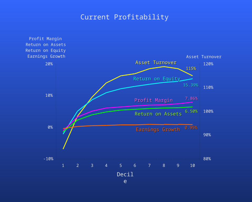
Current Profitability
Asset TurnoverAsset Turnover115%115%
Return on EquityReturn on Equity15.39%15.39%
Profit MarginProfit Margin 7.86%7.86%
Return on AssetsReturn on Assets 6.50%6.50%
90%
100%
110%
120%
Asset Turnover
2 3 4 5 6 7 8 9 10
Decile
80%-10%
0%
10%
20%
1
Profit Margin Return on Assets Return on Equity Earnings Growth
Earnings GrowthEarnings Growth 0.95%0.95%

Trends in Profitability

1 2 3 4 5 6 7 8 9 10
Decile
5 Year Trailing Growth
-1.5%
-1.0%
-0.5%
0.0%
Profitability Trends(Growth In)
Asset TurnoverAsset Turnover
-0.13%-0.13%Profit MarginProfit Margin
-0.95%-0.95% Return on AssetsReturn on Assets
-1.11%-1.11% Return on EquityReturn on Equity
-1.18%-1.18%

Cheapness in Stock Price

Price Level
Sales-to-PriceSales-to-Price214%214%
207%207%
Cash Flow-to-PriceCash Flow-to-Price
6%6%
17%17%
Earnings-to-PriceEarnings-to-Price
-1.55%-1.55%
10%10%
Dividend-to-PriceDividend-to-Price2.19%2.19%
3.69%3.69%
50%
100%
150%
200%
Sales-to-Price Book-to-Price
3 4 5 6 7 8 9 10
Decile
0%-10%
0%
10%
20%
1 2
Cash Flow-to-Price
Earnings-to-Price
Dividend-to-Price
Book-to-PriceBook-to-Price81%81%
80%80%
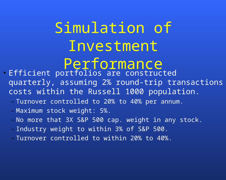
Simulation of Investment Performance
• Efficient portfolios are constructed quarterly, assuming 2% round-trip transactions costs within the Russell 1000 population.– Turnover controlled to 20% to 40% per annum.– Maximum stock weight: 5%.– No more that 3X S&P 500 cap. weight in any stock.– Industry weight to within 3% of S&P 500.– Turnover controlled to within 20% to 40%.

10%11%
12%13%
14%15%
18%
17%
16%
20%
19%
12%
Ann
ualiz
ed to
tal r
etur
n
17% 18%13% 14% 15% 16%
Annualized volatility of return
1000 Index
GI
H
L
Optimized Portfolios in the Russell 1000 Population: 1979-1993Optimized Portfolios in the Russell 1000 Population: 1979-1993
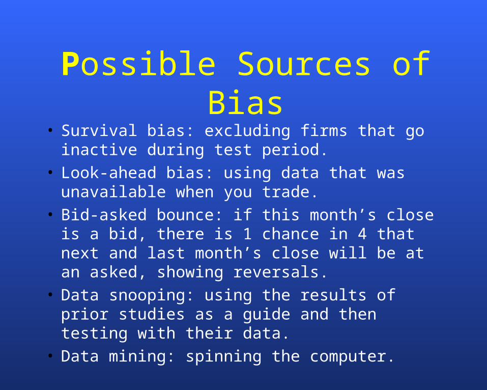
Possible Sources of Bias• Survival bias: excluding firms that go inactive
during test period.• Look-ahead bias: using data that was unavailable
when you trade.• Bid-asked bounce: if this month’s close is a bid,
there is 1 chance in 4 that next and last month’s close will be at an asked, showing reversals.
• Data snooping: using the results of prior studies as a guide and then testing with their data.
• Data mining: spinning the computer.

Using the Ad Hoc Expected Return Factor Model
Internationally• The most important factors across the 5
largest stock markets (1985-93).

Using the Ad Hoc Expected Return Factor Model
Internationally• The most important factors across the 5
largest stock markets (1985-93).
• Simulating investment performance.– Within countries, constraints are those stated
previously.
– Positions in countries are in accord with relative total market capitalization.
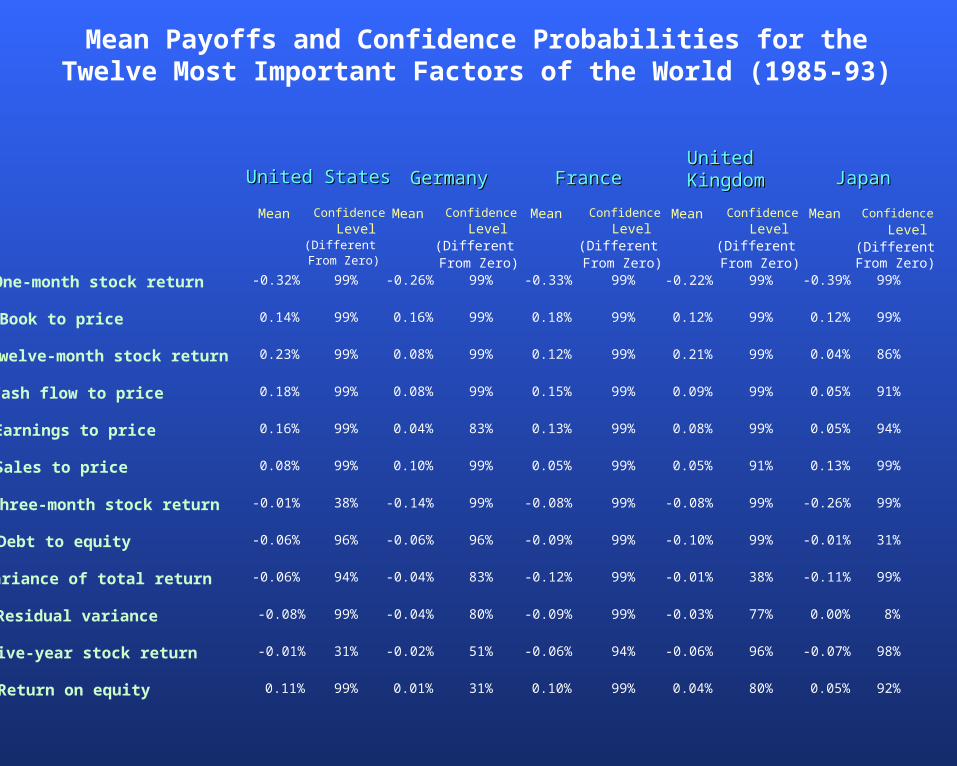
Mean Payoffs and Confidence Probabilities for theTwelve Most Important Factors of the World (1985-93)
One-month stock return
Book to price
Twelve-month stock return
Cash flow to price
Earnings to price
Sales to price
Three-month stock return
Debt to equity
Variance of total return
Residual variance
Five-year stock return
Return on equity
United StatesUnited States
Mean Confidence Level(DifferentFrom Zero)
-0.32% 99%
0.14% 99%
0.23% 99%
0.18% 99%
0.16% 99%
0.08% 99%
-0.01% 38%
-0.06% 96%
-0.06% 94%
-0.08% 99%
-0.01% 31%
0.11% 99%
GermanyGermany
Mean Confidence Level(DifferentFrom Zero)
-0.26% 99%
0.16% 99%
0.08% 99%
0.08% 99%
0.04% 83%
0.10% 99%
-0.14% 99%
-0.06% 96%
-0.04% 83%
-0.04% 80%
-0.02% 51%
0.01% 31%
FranceFrance
Mean Confidence Level(DifferentFrom Zero)
-0.33% 99%
0.18% 99%
0.12% 99%
0.15% 99%
0.13% 99%
0.05% 99%
-0.08% 99%
-0.09% 99%
-0.12% 99%
-0.09% 99%
-0.06% 94%
0.10% 99%
United United KingdomKingdom
Mean Confidence Level(DifferentFrom Zero)
-0.22% 99%
0.12% 99%
0.21% 99%
0.09% 99%
0.08% 99%
0.05% 91%
-0.08% 99%
-0.10% 99%
-0.01% 38%
-0.03% 77%
-0.06% 96%
0.04% 80%
JapanJapan
Mean Confidence Level(Different
From Zero)-0.39% 99%
0.12% 99%
0.04% 86%
0.05% 91%
0.05% 94%
0.13% 99%
-0.26% 99%
-0.01% 31%
-0.11% 99%
0.00% 8%
-0.07% 98%
0.05% 92%
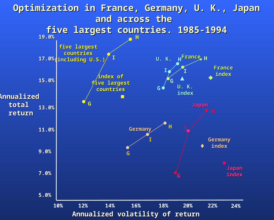
Optimization in France, Germany, U. K., Japan and across the Optimization in France, Germany, U. K., Japan and across the five largest countries. 1985-1994five largest countries. 1985-1994
19.0%19.0%
17.0%17.0%
15.0%15.0%
13.0%13.0%
11.0%11.0%
9.0%9.0%
7.0%7.0%
5.0%5.0%
10% 12% 14% 16% 18% 20% 22% 24%
G
I
HFranceFrance
FranceFranceindexindex
U. K.U. K. H
I
G U. K.U. K.indexindex
GermanyGermany
GermanyGermanyindexindex
H
I
G
JapanJapan
H
I
GG
JapanJapanindexindex
five largest five largest countries countries
(including U.S.)(including U.S.)
H
I
G
index ofindex offive largestfive largestcountriescountries
Annualized Annualized total total
returnreturn
Annualized volatility of returnAnnualized volatility of return

Expansion of the 1996 Study
(Nardin Baker)

Performance In Different Countries: 1985 - 1998 (Sept.)
0%
5%
10%
15%
20%
25%
30%
12% 14% 16% 18% 20% 22% 24% 26% 28% 30% 32%
Volatility
Return
AUS BEL CAN CHE DEU ESP FRA
GBR HKG ITA JPN NLD SWE USA

Actual Performance

Performance before fees, after transactions costs and includes reinvested dividends
Industrif inans Contact: Ole Jakob Wold +47.22.473300 Measured in Norw egian Krone (NOK), Managed to stay neutral in country and sector w eightsPast performance is not a guarantee of future results Managed using modif ied (Haugen-Baker) JFE Expected Return Model by Baker at Grantham Mayo Van Otterloo, Inc.
Industrifinans ForvaltningGlobal Fund
170.65%
144.04%
-20.00%
0.00%
20.00%
40.00%
60.00%
80.00%
100.00%
120.00%
140.00%
160.00%
180.00%
start jan.95 apr jul oct jan.96 apr jul oct jan.97 apr jul oct jan.98 apr jul oct jan.99 apr
Cumulative return since inception (31 October 1994)
Industrifinans WorldMorgan Stanley World NOK

Performance measured before fees, after transactions costs and includes reinvested dividends
Industrif inans Contact: Ole Jakob Wold +47.22.473300 Measured in Norw egian Krone (NOK), Managed to stay neutral in country and sector w eightsPast performance is not a guarantee of future results Managed using modif ied (Haugen-Baker) JFE Expected Return Model by Baker at Grantham Mayo Van Otterloo, Inc.
Industrifinans ForvaltningProbability that the expected return to the Global Fund has been higher than the Morgan Stanley World Index
92.2%
0.0%
10.0%
20.0%
30.0%
40.0%
50.0%
60.0%
70.0%
80.0%
90.0%
100.0%
dec.94 mar jun sep dec.95 mar jun sep dec.96 mar jun sep dec.97 mar jun sep dec.98 mar
Probability of out-performing the Morgan Stanley World Index since inception (31 October 1994)
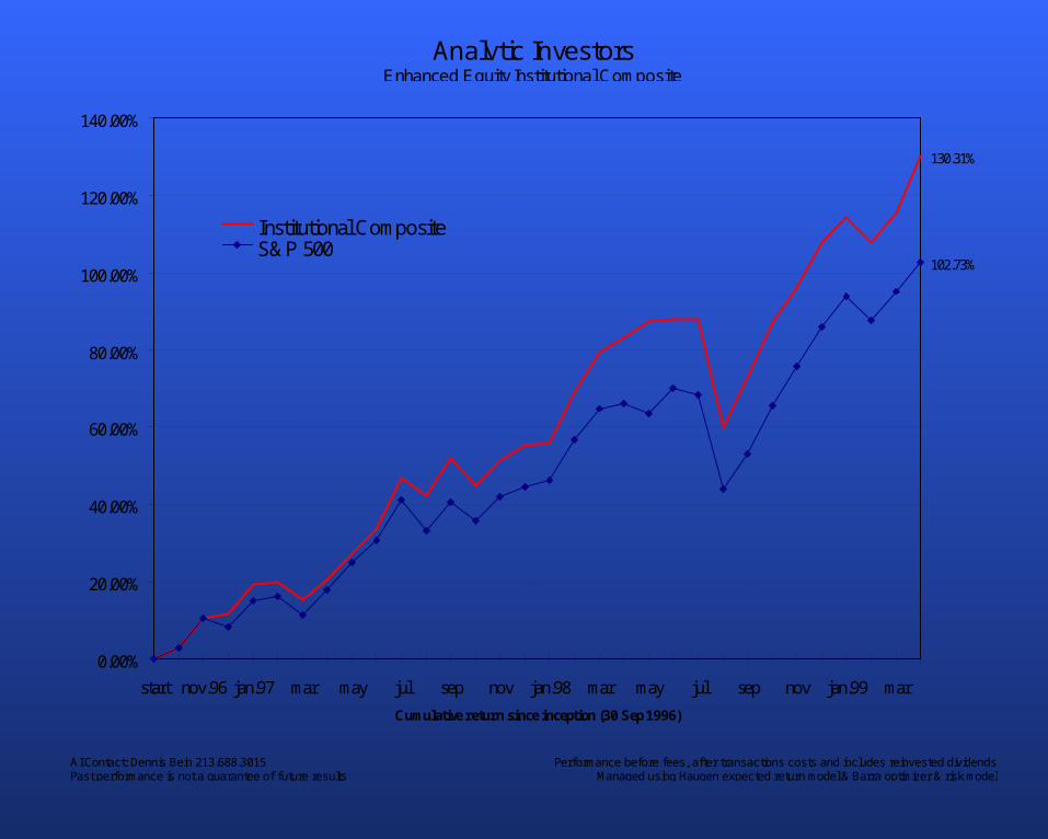
AI Contact: Dennis Bein 213.688.3015 Performance before fees, after transactions costs and includes reinvested dividendsPast performance is not a guarantee of future results Managed using Haugen expected return model & Barra optimizer & risk model
Analytic InvestorsEnhanced Equity Institutional Composite
130.31%
102.73%
0.00%
20.00%
40.00%
60.00%
80.00%
100.00%
120.00%
140.00%
start nov.96 jan.97 mar may jul sep nov jan.98 mar may jul sep nov jan.99 mar
Cumulative return since inception (30 Sep 1996)
Institutional CompositeS&P 500

AI Contact: Dennis Bein 213.688.3015 Performance before fees, after transactions costs and includes reinvested dividendsPast performance is not a guarantee of future results Managed using Haugen expected return model & Barra optimizer & risk model
Analytic InvestorsProbability that the expected return to the Enhanced Equity Institutional Composite has been higher than the S&P 500 Index
93.3%
0.0%
10.0%
20.0%
30.0%
40.0%
50.0%
60.0%
70.0%
80.0%
90.0%
100.0%
nov.96 feb.97 may aug nov feb.98 may aug nov feb.99
Probability of out-performing the S&P 500 Index since inception (30 Sep 1996)

Performance of 413 Mutual Funds 10/96 -
9/98
• “T” stat. on mean monthly out-performance to S&P 500
• Large funds with highest correlation with S&P with a 36 month history

Three YearThree Year OutOut--(Under)(Under)-Performance T-Distribution-Performance T-Distribution
0%0%
5%5%
10%10%
15%15%
20%20%
25%25%
to -5.0 -5.0 to
-4.5
-4.5 to
-4.0
-4.0 to
-3.5
-3.5 to
-3.0
-3.0 to
-2.5
-2.5 to
-2.0
-2.0 to
-1.5
-1.5 to
-1.0
-1.0 to
-0.5
-0.5 to
0.0
0.0 to
0.5
0.5 to
1.0
1.0 to
1.5
1.5 to
2.0
2.0 to
T-statistics for mean T-statistics for mean outout--(under)(under) performance performance
Per
cen
t o
f sa
mp
leP
erce
nt
of
sam
ple
Top Related