


Languages
Pages
Legal


CERDI, Etudes et Documents, E 2012.16
C E N T R E D ' E T U D E S
E T D E R E C H E R C H E S
S U R L E D E V E L O P P E M E N T
I N T E R N A T I O N A L
Document de travail de la série
Etudes et Documents
E 2012.16
The environmental Kuznets curve for deforestation:
a threatened theory? A meta-analysis
Johanna CHOUMERT, Pascale COMBES MOTEL,
Hervé K. DAKPO
avril 2012
CERDI
65 BD. F. MITTERRAND
63000 CLERMONT FERRAND - FRANCE
TEL. 04 73 17 74 00
FAX 04 73 17 74 28
www.cerdi.org

CERDI, Etudes et Documents, E 2012.16
Les auteurs
Johanna Choumert
Associate Professor, Clermont Université, Université d’Auvergne, CNRS, UMR 6587, Centre d’Etudes et de
Recherches sur le Développement International (CERDI), F-63009 Clermont-Ferrand, France
Email : [email protected]
Pascale Combes Motel
Professor, Clermont Université, Université d'Auvergne, CNRS, UMR 6587, Centre d’Etudes et de
Recherches sur le Développement International (CERDI), F-63009 Clermont-Ferrand, France
Email : [email protected]
Hervé K. Dakpo
Student, Clermont Université, Université d'Auvergne, CNRS, UMR 6587, Centre d’Etudes et de Recherches
sur le Développement International (CERDI), F-63009 Clermont-Ferrand, France
Email : [email protected]
Corresponding author: [email protected]
La série des Etudes et Documents du CERDI est consultable sur le site :
http://www.cerdi.org/ed
Directeur de la publication : Patrick Plane
Directeur de la rédaction : Catherine Araujo Bonjean
Responsable d’édition : Annie Cohade
ISSN : 2114-7957
Avertissement :
Les commentaires et analyses développés n’engagent que leurs auteurs qui restent seuls
responsables des erreurs et insuffisances.

CERDI, Etudes et Documents, E 2012.16
Highlights • We carry out a meta-analysis of Environmental Kuznets Curve (EKC) studies for
deforestation. • We analyze the results of 71 studies, offering a total of 631 estimations. • We investigate the incidence of choices made by authors (econometric strategy,
deforestation measure, temporal coverage, geographical area, measure of economic development…) on the probability of finding an EKC.
• After a phase of work corroborating the EKC, we find a turning point after the year 2001.
Abstract
Although widely studied, deforestation remains a topical and typical issue. The relationship
between economic development and deforestation is still at stake. This paper presents a meta-
analysis of Environmental Kuznets Curve (EKC) studies for deforestation. Using 71 studies,
offering 631 estimations, we shed light on why EKC results differ. We investigate the incidence
of choices made by authors (econometric strategy, deforestation measure, temporal coverage,
geographical area, measure of economic development…) on the probability of finding an EKC.
After a phase of work corroborating the EKC, we find a turning point after the year 2001.
Building on our results, we conclude that the EKC story will not fade until theoretical
alternatives will be provided.
Keywords
Meta-Analysis; Environmental Kuznets Curve; Deforestation, Development
JEL Codes
C12, C83, Q23, O13
CERDI, Etudes et Documents, E 2012.16
1
Mark Twain: “The report of my death was an exaggeration”
New York Journal 2 June 1897
1. Introduction
One important question which is still at stake, even more in an economic crisis
context, is whether environmental and economic objectives are compatible subjects.
This question gets high resonance in the literature devoted to the Environmental
Kuznets Curve (EKC) for deforestation which is a subject of confrontation between
optimistic and pessimistic views of development (Carson 2010). This literature has
gained considerable expansion in economics as well as in natural sciences (Mather et al.
1999). From the 1990s onwards, numerous studies following the idea of (Grossman &
Krueger 1995) tested an EKC for deforestation.
Studying EKCs for deforestation is an important matter for two reasons.
First, forest depletion has been given increasing attention especially with the
recognition of the role of forests in the global carbon cycle. Recent developments in the
literature on climate change put forward the potential role of forests in climate change
mitigation (N. H. Stern 2007). The impetus was given to the so-called “Reducing
emissions from deforestation and forest degradation” (REDD) device first proposed for
negotiation at the Montreal UNFCCC CoP held in 2005. The Bali Road Map adopted in
2007 went beyond with the REDD+ concept by enhancing other objectives such as
sustainable management of forests and valuation of forests carbon stocks (Angelsen,
Brockhaus, et al. 2009; Angelsen, Brown, et al. 2009; Engel & Palmer 2008). As pointed
out by (Geist & Lambin 2001) the role of forests in mitigating global environmental
threats such as climate change and biodiversity erosion is a research imperative and has
been motivating considerable efforts to the understanding of patterns and causes of the
CERDI, Etudes et Documents, E 2012.16
2
deforestation process and in fine to the derivation of policy implications (Angelsen &
Kaimowitz 1999).
Second, EKC has drawn attention from scholars for several years (e.g. (Ma & D. I.
Stern 2006). Studying EKCs for deforestation may therefore offer an interesting case in
the methodology of economics from a sociological point of view. According to (Kuhn
1996), scientists share common beliefs and practices which circumscribe the “normal
science”. They are often reluctant to diverge from them since they are most of the time
evaluated and published according to rules widely accepted within the normal science.
EKCs seem to belong to such a set of practices. It is indeed rather striking that several
researchers seem to consider it as “econometrics as usual” i.e. a relevant hypothesis
which helps understanding environmental degradation and for instance the
deforestation process. Other researchers have conducted critical reviews and forcefully
argued in favour of its obsolescence (Levinson 2002; D. I. Stern 2004). Thus there seems
to be a discrepancy between, on the one side, researchers who dismiss EKCs and, on the
other side, scientists who consider that EKCs are relevant. Among the latter, the EKC is
still presented as one of the hypotheses explaining the forest transition process (Barbier
et al. 2010; Rudel et al. 2005; Mather 1992).
The objective of this paper is to examine why scholars get accustomed to the EKC for
deforestation or whether they have “objective” reasons to dismiss it. In contrast with
existing studies or critical surveys on the EKC for deforestation, we propose to address
the subject with a meta-analysis which can be considered as an attempt to identify
“wheat from chaff” (Stanley 2001) i.e. identify a set of reasons that favour or falsify
empirical evidences of EKCs for deforestation.

CERDI, Etudes et Documents, E 2012.16
3
The rest of the paper is organised as follows. Section 2 presents the debate in the
literature on the EKC for deforestation. Section 3 further justifies the use of meta-
analysis. Section 4 is devoted to the construction of the database. Section 5 develops on
the empirical strategy and the econometric results. Section 6 discusses the results and
Section 7 concludes.
2. Contrasted Premises and Results
The story with EKCs started with (Grossman & Krueger 1995) and (Panayotou 1993).
According to (Beckerman 1992, p.482) : “[…] there is clear evidence that, although
economic growth usually leads to environmental deterioration in the early stages of the
process, in the end the best - and probably the only - way to attain a decent environment
in most countries is to become rich.” This optimistic premise was later mitigated by the
(Arrow et al. 1996) assertion according to which economic growth is not a sufficient
condition for getting environmental improvements or curbing environmental
degradation. It is even more doubtful to find EKCs when stock variables with strong
potential feedback are expected in, for instance, ecosystems such as tropical forests.
The economic literature provides theoretical underpinnings for an EKC. Many of them
model pollutants emissions – income relationships (Andreoni & Levinson 2001;
Xepapadeas 2005). (Munasinghe 1999) develops a static model showing that
appropriate policy measures (i.e. removal of subsidies on timber exports) could help
alleviating the pressure on tropical forest stocks and thus “tunnelling” through the EKC
for deforestation. Theoretical explanations of EKCs for deforestation were also
developed with the so-called poverty-environment hypothesis as opposed to the capital
or frontier model (Geist & Lambin 2001; Rudel & Roper 1997). The contention that
economic development has a negative (positive) impact on deforestation is suggested by
CERDI, Etudes et Documents, E 2012.16
4
the former (latter). Theoretical models explaining agricultural land expansion may also
be compatible with an EKC for deforestation (Barbier 2001). It is however worth to
notice that several authors are rather unsatisfied with the current theoretical literature
on the EKC for deforestation and call for further developments (Roy Chowdhury &
Moran 2012).
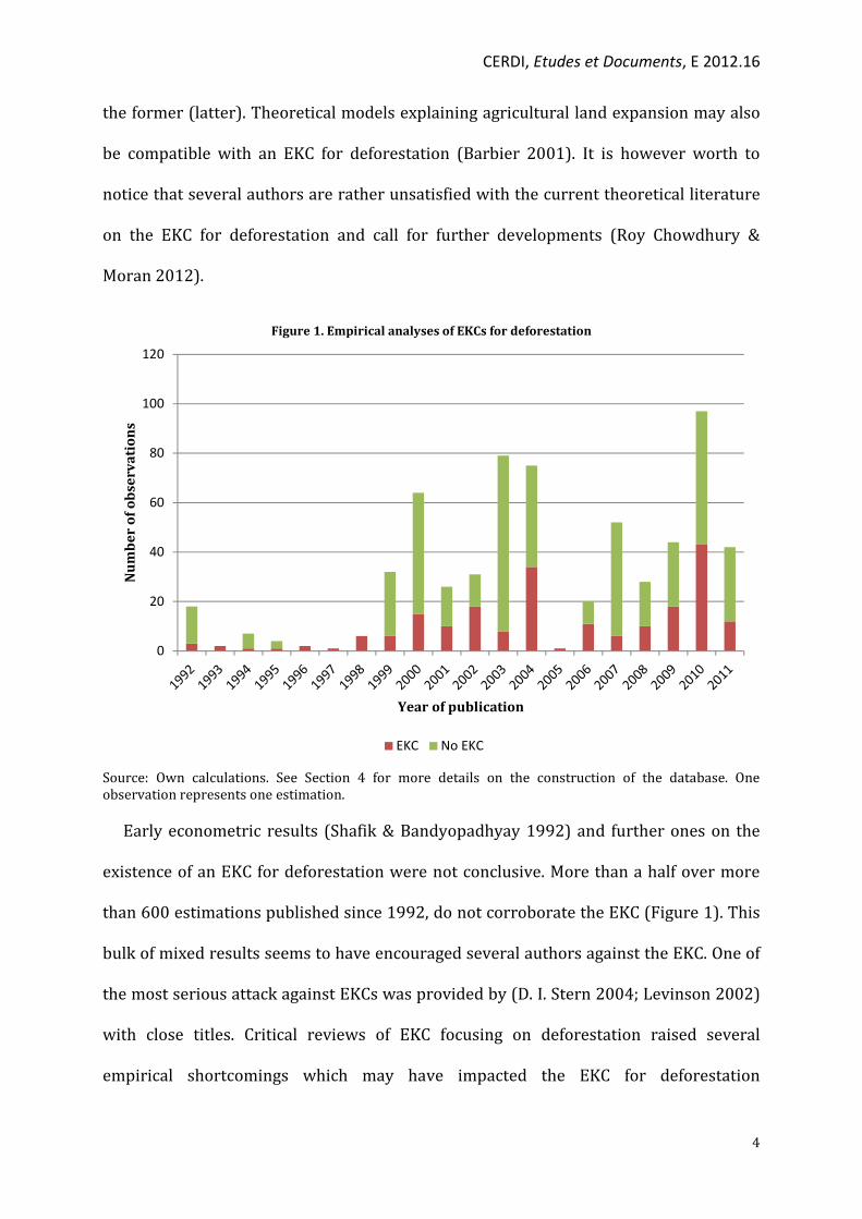
Figure 1. Empirical analyses of EKCs for deforestation
Source: Own calculations. See Section 4 for more details on the construction of the database. One observation represents one estimation.
Early econometric results (Shafik & Bandyopadhyay 1992) and further ones on the
existence of an EKC for deforestation were not conclusive. More than a half over more
than 600 estimations published since 1992, do not corroborate the EKC (Figure 1). This
bulk of mixed results seems to have encouraged several authors against the EKC. One of
the most serious attack against EKCs was provided by (D. I. Stern 2004; Levinson 2002)
with close titles. Critical reviews of EKC focusing on deforestation raised several
empirical shortcomings which may have impacted the EKC for deforestation
0
20
40
60
80
100
120
Nu
mb
er
of
ob
serv
ati
on
s
Year of publication
EKC No EKC
CERDI, Etudes et Documents, E 2012.16
5
corroboration. As mentioned by (Koop & Tole 1999), FAO databases were mostly used.
Early FAO databases were from FAO production yearbook. Supposedly, more recent
ones from Forest Resources Assessment published in most recent studies have greater
reliability. Irrelevant econometric methods are also put forward. Early estimates relied
on cross-section data which imply restrictive hypotheses (Dinda 2004; Koop & Tole
1999). More recent studies thus implemented panel data or more generally pooled cross
sectional time series data. It may be worth to examine whether improvements made in
econometric devices had an impact on the existence of an EKC for deforestation.
One may thus be confused between on the one side, Stern's contention according to
which “most of the EKC literature is econometrically weak” (D. I. Stern 2004, p.1420)
and empirical analyses still relying on or testing the EKC for deforestation. But one may
understand the situation while remembering (McCloskey 1983). It seems that
economists need more than statistical tests to get rid of a hypothesis like the EKC. Would
they give weight to the rhetoric surrounding the EKC? In this paper, we want to check
whether characteristics of publications dealing with EKCs for deforestation play a role in
their corroboration. We argue that conducting a meta-analysis of EKCs for deforestation
equations can contribute to their critical assessment.
3. The Use of Meta-Analysis
A meta-analysis produces, through a set of statistical techniques, an overall summary
of empirical knowledge on a specific topic. “Meta-analysis is the analysis of empirical
analyses that attempts to integrate and explain the literature about some important
parameter” (Stanley & Jarrell 1989, in (Stanley et al. 2008, p.163). “It can explain the
excess study-to-study variation typically found in empirical economics, uncover the
trace of statistical power that is associated with a false theory, and see through the

CERDI, Etudes et Documents, E 2012.16
6
distortion of publication selection and misspecification biases” (Stanley 2005, in
(Stanley et al. 2008, p.163).
Before the 90's, scientists synthesised the results of the research literature through
the use of narrative review. However, the limit of this method was quickly reached with
the increase in the amount of information available. Indeed it seems inconceivable using
this method to successfully synthesize the results of dozens of studies which, moreover,
are conflicting in their results. (Hunter & Schmidt 2004) explain that narrative surveys
developed the so-called “myth of the perfect study”: a researcher may be convinced that
some studies suffer from methodological flaws and exclude them from the review;
another one may consider different methodological flaws. Hence, idiosyncratic ideas
may lead one to reduce available literature on a topic from 100 studies to 10 and
another one from 100 to 50.
Meta-analysis allows to address the inherent limitations of the traditional narrative
review by providing a more effective approach (Stanley 2001); it allows to set up an
evaluation with several measures of “outcome”; it permits the use of moderators: some
characteristics of the samples used in different studies influence the results obtained.
Moreover, meta-analysis is a good tool for decision support because it helps in the
assistance in planning, in the generation of new hypotheses, and eventually, prospective
meta-analysis.
Research questions are often the subject of numerous studies leading to various
controversies. As mentioned earlier, the EKC for deforestation is no exception, on the
contrary, as shown in different reviews of the literature on the subject. Different
opinions differ on the question of the existence of an EKC for deforestation and this,
especially since empirical analysis validate and invalidate this hypothesis according to

CERDI, Etudes et Documents, E 2012.16
7
econometric models, measures of deforestation, study area, temporal coverage, etc.
Since 1992, empirical work has been accumulated and we even see a significant increase
in the number of studies since the 2000s (Figure 1). Finally, despite the abundance of
empirical studies, it is difficult to propose clear recommendations arising directly from
the relationship between economic growth and deforestation. Our approach, based on
the meta-analysis, is complementary with respect to existing surveys (D. I. Stern et al.
1996; D. I. Stern 2004; Dinda 2004). Indeed, it allows us to statistically analyse the
variation in results found between existing works and in particular to analyse the
influence of choices made by the authors on their results (Stanley 2001).
There exists meta-analysis for EKC studies. These encompass however various
environmental goods. (Cavlovic et al. 2000) performed a meta-analysis of 25 studies -
121 observations - with a focus on turning points. They cover 11 categories of
environmental goods such as urban air quality or deforestation. Observations for
deforestation represent only 6 % of their sample. The impact of deforestation on income
turning points depends on the econometric specification of the meta-analysis. (Jordan
2010) analyses 255 articles - 373 observations - among which 8 % deal with
deforestation. Results show no significant impact of deforestation on the probability of
finding an EKC.
The operationalization of a meta-analysis is done by following specific steps. The first
step is the formulation of the subject: what are the issues and objectives of the study
(central questions we would like answers to) and what are the assumptions made. The
second step is the overall design of the study: this is to clarify outcomes, populations,
settings, criteria for inclusion and exclusion of studies. The third step is to specify the
sampling plan, the units of observation and then begin the literature search. The fourth

CERDI, Etudes et Documents, E 2012.16
8
step is the extraction of data: it is directly applicable to studies that were selected for
further analysis after the application of inclusion / exclusion criteria. The fifth step is the
statistical analysis. As recommended by (Nelson & Kennedy 2008), we address relevant
issues such as heteroskedasticity, the non-independence of regressions, the specification
of the model, the non-normality of residuals and multicollinearity.
4. Construction of the Database
4.1. Sampling procedure and sample characteristics
This meta-analysis is based on 71 studies, offering 631 estimations.1 In a meta-
analysis, an important aspect of the work is to find studies that addressed the theme of
the investigation. We conducted our research using academic databases such as “Science
Direct”, “Springer”, “RePEc Ideas”, “Mendeley”, “Wiley”, etc. The first step of this research
was to enter keywords such as “Kuznets AND Deforestation”, “Income AND
Deforestation”, “Development AND Deforestation”, “Poverty AND Deforestation”. Given
that there are relevant studies which are not identified by bibliographic databases, in a
second step we carried out a manual search and this by identifying journals and articles
relevant to the topic. We then browsed these studies in order to identify new ones which
have addressed closely the subject. A third step was necessary as we had to directly
contact the authors since some studies are not accessible on the web. At the end of the
research process, we got to build up an information base of nearly 102 items that we
have then filtered through inclusion criteria.
At this stage, we selected eligibility criteria to be applied to the bibliographic
database. In order not to bias the meta-analysis on subjective considerations, we tried to
be broad in our inclusion criteria. First, we looked closely at the dependent variable
1 The list of primary studies is available from the authors upon request (See Table A - 1 in the Appendix).

CERDI, Etudes et Documents, E 2012.16
9
used in each estimation. Once done, we decided to retain all the measures relating
directly to deforestation. At the end of this inclusion work, we have reached 71 studies
that were used to build the database of this article.2
Every relevant estimation was carefully examined and the information was gathered
to build the database. Accordingly, we surveyed all the information given by the authors
related to the EKC (coefficients associated with variables of interest), the sample (size,
geographical area …), the econometric method, control variables, and all information
considered necessary to carry out this meta-analysis. In terms of coefficients and their
sign, they were adjusted according to the nature of the dependent variable and
depending on the outcome. For example, when the dependent variable is the rate of
deforestation, to obtain an EKC, the coefficient of per capita GDP should be positive and
negative for the squared GDP. By cons, if the dependent variable is the stock of forest,
the hypothesis of an EKC is confirmed if the coefficient of GDP is negative and that of
squared GDP is positive. Also to be as broad as possible we defined our null hypothesis
whenever the estimated marginal effects of GDP and GDP squared had the expected
signs at the 10% level.3 We did not try to minimise this type I error since it is
detrimental to the power of the test. In brief, we define our dependent variable as EKC
which equals to 1 when the existence of the EKC for deforestation is corroborated and 0
otherwise.
2 For instance were excluded from the sample studies analyzing biodiversity, the ecological footprint, land vulnerability or protected areas. Also studies focusing on households were excluded.
3 The decision on the results was based on the significance of all coefficients of interest. For instance, in the quadratic model, as in most studies tests for joint significance were not performed, the model is considered significant if the two coefficients (i.e. per capita GDP and squared per capita GDP) are individually significant.

CERDI, Etudes et Documents, E 2012.16
10
4.2. Moderator variables
At the end of this work, the database we had raw on hand included 631 observations
and numerous differences, most of which focused on the explanatory variables used.
Therefore for the sake of synthesis, these variables were grouped into classes. Table 1
presents the description and descriptive statistics of the variables. Next we shall discuss
factors that may affect the income-deforestation relationship. These are the explanatory
variables used in our model.
In view of the criticisms of the EKC literature, our variables of interest are the year of
publication and the econometric technique.
Regarding the time period, variables are the year of publication of the study, the
initial year of data, the final year of data. Differences between studies may reflect
numerous issues such an academic trend, the increasing quality and availability of
deforestation data, the mix of old and recent data or econometric requirements in peer-
reviewed journals. For instance, (Jordan 2010) finds that the most recent year of
publication is, the more likely to find an EKC decreases, while controlling for the nature
of environmental degradation.
With respect to econometric techniques, as pointed out in critical reviews of EKCs,
one may cast doubts on econometric techniques in early works. Advances in
econometrics may make recent studies more credible than they were in the nineties.
Several authors argued for instance that panel data regressions are more appropriate
for analysing the EKC. Indeed, deforestation is a dynamic process therefore the nature of
the relationship between income and deforestation should also be dynamic. If the time
dimension is ignored, a spurious income-deforestation relationship could be observed.
(Dinda 2004) argues that cross-section analysis is based on restrictive econometric

CERDI, Etudes et Documents, E 2012.16
11
assumptions as to admit the same constant. What is more, using panel data also allows
for controlling for substantial time-invariant unobservable variables (such as countries
physical characteristics or historical factors among many others). On top of that, the EKC
theory was developed in an a-spatial framework. Hence, we could expect the inclusion of
spatial dimension to alter the EKC hypothesis.
In addition to the variables of interest, we propose control variables or moderators.
Concerning the measures of deforestation, we note that in early studies, the latter is not
homogeneous. As part of this work 15 different measures are used. It is interesting to
investigate whether these modify the income-deforestation relationship. In fact, some
measures of deforestation are causes of the latter, as the expansion of agricultural land
or infrastructures. (Geist & Lambin 2001) illustrate the differentiated effects of different
causes of deforestation. We also believe relevant to include the geographical area; in fact
growth path are different in developed and developing countries which can influence
the occurrence of EKC and even more so that the samples of studies are based on recent
data that do not capture development phases of developed countries. As for the
measures of economic development, we observe some heterogeneity in the sample.
However, there is no a priori on why and in what way such differences affect the
occurrence of an EKC. Regarding the publication type, according to the aim of the study,
one can expect different strategies of the authors, without compromising their
neutrality. In particular, as Lindhjem (2007) finds a significant effect of master’s thesis
in his meta-analysis, we can also expect an effect of this publication type. In our case, we
suspect that Master students have less incentive to find an EKC, ceteris paribus. We also
include the presence of control variables for inequalities, life expectancy4 and
4 Life expectancy is correlated with environmental quality (Mariani et al. 2010).

CERDI, Etudes et Documents, E 2012.16
12
infrastructures. We expect the inclusion of these variables to alter the income-
deforestation relationship. In fact, they are correlated with income and this may rise
collinearity issues or shed light on transmission channels. Finally we add other sources
of variation namely the sample size, the h-index of the publication,5,6 the type of model
estimated (quadratic or cubic) and the number of regressions presented.7,8
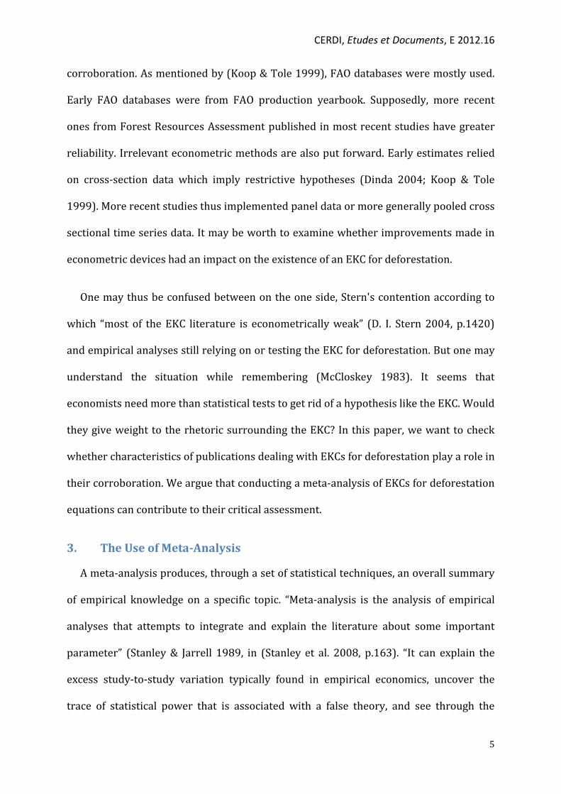
Table 1. Description and descriptive statistics of variables
Variables Description Mean SD Min Max
EKC = 1 if an EKC is found, 0 otherwise 0.330 0.470
Year Publication year 2004.582 4.705 1992 2011
initial data Initial year of data 1978.182 12.908 1948 2006
end data Final year of data 1997.403 5.475 1984 2010
sample size Sample size 73.643 211.526 4 2619
H index H index of the publication 0.518 0.412 0.000286 1.000286
reg Number of regressions presented in the study 24.324 19.81 1 60
Measures of deforestation
deforestation1 = 1 if Agricultural land expansion rate, 0 otherwise 0.019 0.137
deforestation2 = 1 if Arable land area, 0 otherwise 0.016 0.125
deforestation3 = 1 if Built-up land, 0 otherwise 0.005 0.069
deforestation4 = 1 if Crop Area, 0 otherwise 0.040 0.195
deforestation5 = 1 if Deforestation, 0 otherwise 0.777 0.417
deforestation6 = 1 if Forest area clearcut, 0 otherwise 0.013 0.112
deforestation7 = 1 if Forest stock, 0 otherwise 0.071 0.258
deforestation8 = 1 if Land use for fuel wood, charcoal, paper, and pulp, 0 otherwise
0.005 0.069
deforestation9 = 1 if Land use for pasture, 0 otherwise 0.005 0.069
deforestation10 = 1 if Land use to produce timber, 0 otherwise 0.005 0.069
deforestation11 = 1 if Mangrove deforestation index, 0 otherwise 0.006 0.079
deforestation12 = 1 if Paved roads in forest regions, 0 otherwise 0.029 0.167
deforestation13 = 1 if Roads encroaching on forest cover, 0 otherwise 0.006 0.079
5 The lower, the better
6 This ranking is done by “Ideas Repec”. At the date of last visit, journals were ranked from 1 to 3 496. So we calculated a ratio that is equal to the rank of the journal divided by the rank of the last journal listed (i.e. 3 496). However for studies that did not receive a ranking on this site, the ratio calculation was made assuming that the rank of this study will be equal to the rank of the last journal classified to which was added one.
7 Note that few studies provide tests to compare models. It is therefore not possible to provide a single regression per article.
8 Other information was collected from studies but was excluded due to collinearity issues such as the unit for the deforestation measure, the source of data for deforestation, etc.
CERDI, Etudes et Documents, E 2012.16
13
Variables Description Mean SD
deforestation14 = 1 if Timber harvest rate, 0 otherwise 0.002 0.040
deforestation15 = 1 if Urban forest canopy percentage, 0 otherwise 0.003 0.056
Econometric techniques
econometrics1 = 1 if Dynamic Panel, 0 otherwise 0.016 0.125
econometrics2 = 1 if Geographically Weighted Regression, 0 otherwise 0.003 0.056
econometrics3 = 1 if Least Absolute Deviation, 0 otherwise 0.002 0.040
econometrics4 = 1 if Logistic Panel Smooth Transition Regression, 0 otherwise 0.016 0.125
econometrics5 = 1 if Monte Carlo Estimation, 0 otherwise 0.006 0.079
econometrics6 = 1 if Ordinary Least Squares, 0 otherwise 0.434 0.496
econometrics7 = 1 if Panel Fixed Effects, 0 otherwise 0.387 0.487
econometrics8 = 1 if Panel Random Coefficients, 0 otherwise 0.013 0.112
econometrics9 = 1 if Panel Random Effects, 0 otherwise 0.082 0.275
econometrics10 = 1 if Spatial Panel Fixed Effects, 0 otherwise 0.019 0.137
econometrics11 = 1 if Spatial Panel Random Effects, 0 otherwise 0.013 0.112
econometrics12 = 1 if Time Series, 0 otherwise 0.010 0.097
fe_retain = 1 if Panel Fixed Effects chosen with Hausman test, 0 otherwise 0.371 0.483
re_retain = 1 if Panel Random Effects chosen with Hausman test, 0 otherwise 0.043 0.203
Geographical areas
area1 = 1 if Africa, 0 otherwise 0.043 0.203
area2 = 1 if Africa and Asia, 0 otherwise 0.014 0.119
area3 = 1 if Africa, Asia, North America, Latin America and Oceania, 0 otherwise 0.019 0.137
area4 = 1 if Africa, Asia, North America and Oceania, 0 otherwise 0.006 0.079
area5 = 1 if Africa, Asia and Latin America, 0 otherwise 0.301 0.459
area6 = 1 if Africa, Asia, Latin America and Europe, 0 otherwise 0.008 0.089
area7 = 1 if Africa, Asia, Latin America and Oceania, 0 otherwise 0.006 0.079
area8 = 1 if Asia, 0 otherwise 0.086 0.280
area9 = 1 if Asia and Latin America, 0 otherwise 0.070 0.255
area10 = 1 if Europe, 0 otherwise 0.024 0.152
area11 = 1 if Latin America, 0 otherwise 0.073 0.260
area12 = 1 if North America, 0 otherwise 0.022 0.147
area13 = 1 if World, 0 otherwise 0.328 0.470
Economic development measures
development1 = 1 if GDP, 0 otherwise 0.642 0.480
development2 = 1 if GNP, 0 otherwise 0.068 0.252
development3 = 1 if Household median income, 0 otherwise 0.003 0.056
development4 = 1 if Human Development Index, 0 otherwise 0.165 0.371
development5 = 1 if Per capita consumption, 0 otherwise 0.011 0.105
development6 = 1 if Poverty, 0 otherwise 0.010 0.097
development7 = 1 if Urbanization, 0 otherwise 0.101 0.302
Publication types
pub type1 = 1 if Article, 0 otherwise 0.498 0.500
pub type2 = 1 if Conference Paper, 0 otherwise 0.024 0.152
pub type3 = 1 if Discussion Paper, 0 otherwise 0.013 0.112
pub type4 = 1 if Other, 0 otherwise 0.166 0.373

CERDI, Etudes et Documents, E 2012.16
14
pub type5 = 1 if Working Papers, 0 otherwise 0.300 0.458
Presence of control variables
life expectancy = 1 if life expectancy variable, 0 otherwise 0.002 0.040
inequality = 1 if inequality variable, 0 otherwise 0.024 0.152
infrastructures = 1 if infrastructures variable, 0 otherwise 0.063 0.244
Others
cubic = 1 if Cubic model, 0 otherwise .0443 0.206
quadratic = 1 if Quadratic model, 0 otherwise 0.956 0.206
N = 631
5. Empirical Strategy and Results
Our response variable is a binary variable "EKC".9 Recall that we investigate the
factors that influence the occurrence of an EKC.10 We first estimate the model using
robust ordinary least squares.11 Indeed, in the presence of a binary dependent variable,
if the model is estimated by OLS, the errors are heteroskedastic. Therefore, it is
appropriate to make a robust estimation with White-corrected standard errors.
Furthermore, given that there may be a within-study autocorrelation leading to the
dependence of regressions within one article, we ran OLS with cluster-robust
inference.12 The reason is that each study estimates various regressions with different
units of measures (cf. Table 2). Then, we perform a bootstrap to deal with non-normality
of residuals and to get reliable standard errors.
9 In the field of environmental economics, the use of a binary criterion into a meta-analysis was used, among others, by (Jeppesen et al. 2002; Schläpfer 2006; Jacobsen & Hanley 2008; Kiel & Williams 2007; Jordan 2010)
10 It is important to note that, in this paper, we do not look into “effects size” which would imply using the income associated with turning points.
11 Several authors recommend running OLS when a binary variable is the endogenous regressor. See (Angrist 2001) for more details.
12 Standard errors are clustered by each study. Such approach has been used, for instance, by (Barrio & Loureiro 2010).
CERDI, Etudes et Documents, E 2012.16
15
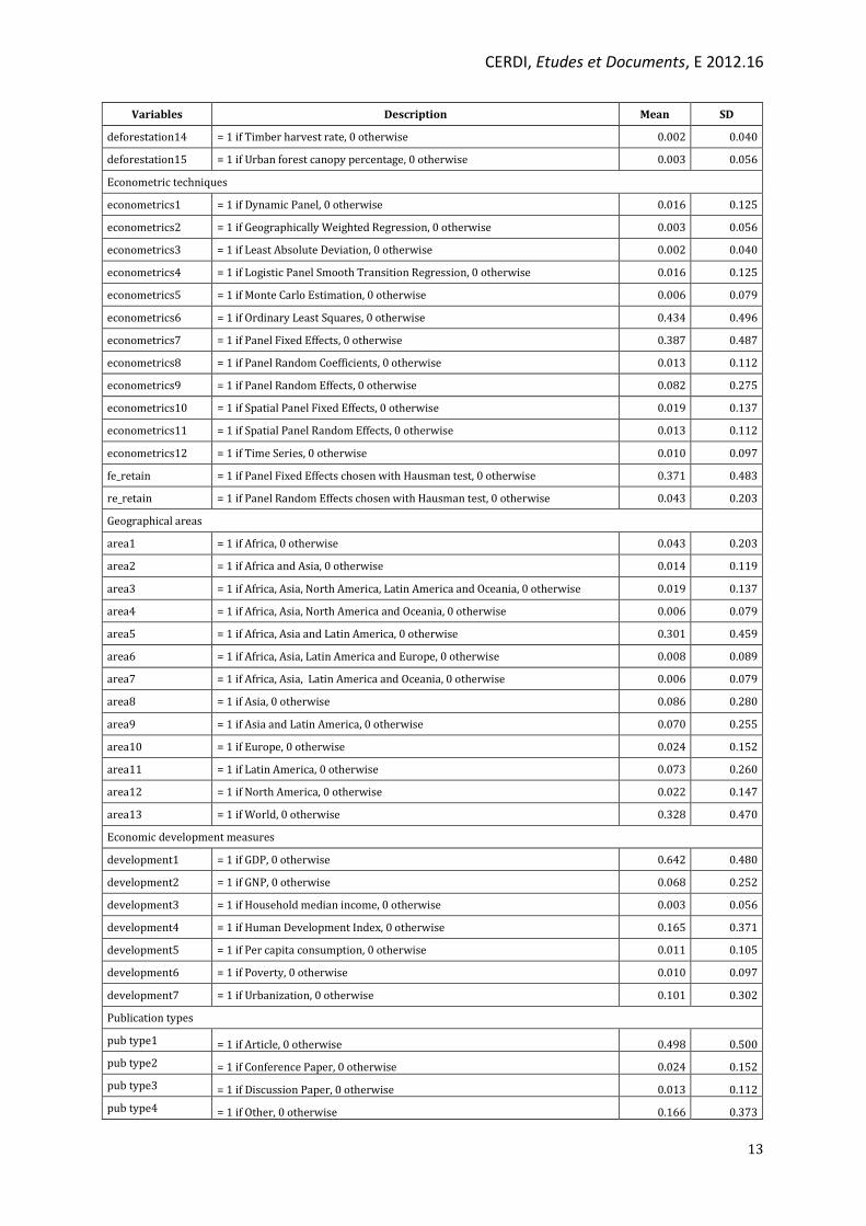
Table 2. Robust OLS equations
VARIABLES OLS robust OLS cluster-robust Boostrap OLS cluster-
robust
year -0.0220** -0.0220 -0.0220*** (0.00997) (0.0160) (0.00812) initial data 0.00591** 0.00591 0.00591*** (0.00276) (0.00495) (0.00218) end data 0.0111 0.0111 0.0111 (0.00947) (0.0151) (0.00763) sample size 0.000474*** 0.000474*** 0.000474*** (6.13e-05) (9.72e-05) (4.70e-05) H index -0.0686 -0.0686 -0.0686 (0.0799) (0.170) (0.0495) deforestation2 0.483 0.483* 0.483* (0.295) (0.272) (0.249) deforestation3 -0.468*** -0.468** -0.468*** (0.130) (0.184) (0.117) deforestation5 -0.0203 -0.0203 -0.0203 (0.111) (0.158) (0.0909) deforestation6 -0.364** -0.364* -0.364*** (0.149) (0.211) (0.123) deforestation7 -0.188 -0.188 -0.188 (0.154) (0.246) (0.123) deforestation8 -0.468*** -0.468** -0.468*** (0.130) (0.184) (0.119) deforestation9 -0.135 -0.135 -0.135 (0.293) (0.184) (0.334) deforestation10 -0.135 -0.135 -0.135 (0.293) (0.184) (0.340) deforestation11 0.559*** 0.559** 0.559*** (0.175) (0.252) (0.146) deforestation12 -0.0653 -0.0653 -0.0653 (0.162) (0.184) (0.146) deforestation13 -0.410*** -0.410* -0.410*** (0.143) (0.223) (0.127) deforestation14 0.477*** 0.477* 0.477*** (0.162) (0.269) (0.126) econometrics1 0.140 0.140 0.140 (0.159) (0.180) (0.162) econometrics2 -0.684*** -0.684*** -0.684*** (0.165) (0.204) (0.147) econometrics3 0.623*** 0.623** 0.623*** (0.137) (0.255) (0.109) econometrics6 -0.0403 -0.0403 -0.0403 (0.0795) (0.0984) (0.0732) fe_retain 0.0940 0.0940 0.0940 (0.0814) (0.0868) (0.0739) econometrics8 -0.435*** -0.435*** -0.435*** (0.113) (0.143) (0.114) re_retain -0.103 -0.103 -0.103 (0.126) (0.144) (0.114) econometrics10 -0.406*** -0.406*** -0.406*** (0.0920) (0.121) (0.0853) econometrics11 -0.406*** -0.406*** -0.406*** (0.0932) (0.121) (0.0868) econometrics12 0.181 0.181 0.181 (0.257) (0.307) (0.182) area1 0.0487 0.0487 0.0487 (0.0949) (0.146) (0.0859) area2 -0.273** -0.273 -0.273** (0.122) (0.236) (0.124) area3 -0.590*** -0.590*** -0.590*** (0.0724) (0.112) (0.0670) area4 -0.588*** -0.588*** -0.588*** (0.0723) (0.112) (0.0669) area5 0.103* 0.103 0.103** (0.0570) (0.122) (0.0454) area6 -0.00590 -0.00590 -0.00590 (0.240) (0.114) (0.253) area8 -0.0388 -0.0388 -0.0388 (0.0833) (0.136) (0.0694) area10 0.0532 0.0532 0.0532

CERDI, Etudes et Documents, E 2012.16
16
(0.151) (0.159) (0.142) area11 0.135 0.135 0.135 (0.0962) (0.191) (0.0867) area12 -0.117* -0.117 -0.117** (0.0638) (0.0877) (0.0592) development1 0.140** 0.140 0.140*** (0.0656) (0.131) (0.0498) development3 0.661*** 0.661*** 0.661*** (0.140) (0.200) (0.118) development5 0.302* 0.302 0.302* (0.176) (0.186) (0.182) pub type1 0.0232 0.0232 0.0232 (0.0733) (0.138) (0.0528) pub type2 -0.234 -0.234 -0.234 (0.220) (0.244) (0.163) pub type3 -0.250** -0.250 -0.250*** (0.124) (0.191) (0.0946) pub type4 -0.240** -0.240 -0.240*** (0.107) (0.184) (0.0821) life expectancy -0.195* -0.195* -0.195** (0.109) (0.114) (0.0978) Inequality 0.504*** 0.504** 0.504*** (0.150) (0.201) (0.0876) Infrastructures -0.352*** -0.352** -0.352*** (0.106) (0.170) (0.0781) quadratic 0.251** 0.251** 0.251*** (0.106) (0.107) (0.0868) reg 0.000892 0.000892 0.000892 (0.00198) (0.00287) (0.00165) Constant 10.35 10.35 10.35 (11.22) (25.74) (8.122) Observations 631 631 631 R-squared 0.242 0.242 0.242
Robust standard errors in parentheses; *** p<0.01, ** p<0.05, * p<0.1
Due to the high number of variables available – some being redundant – in a meta-
analysis, multicollinearity is a serious concern. Recall that multicollinearity leads to
unstable coefficients and inflated standard errors. We use Variance Inflation Factors
(VIFs) to detect it (cf. Table 3). Different views exist on the threshold to accept. Some
argue that VIFs should not go beyond 30; others adopt a more strict value of 10. As
shown in Table 3, VIF values do not exceed 10. What is more, the mean of VIFs is not
considerably larger than 1, which goes in line with the most conservative rule of thumb
(Chatterjee & Hadi 2006). We then perform the Ramsey’s RESET test, on robust OLS, in
order to check for omitted variables and model misspecification.13
13 We find that F(3, 578) = 1.23 with Prob > F = 0.2981. Therefore there is no omitted variable / misspecification issue in the model.

CERDI, Etudes et Documents, E 2012.16
17
Table 3. Variance Inflation Factors
Variables VIF
end data 7.28 infrastructures 2.12 econometrics11 1.33
econometrics6 6.37 re_retain 2.12 econometrics2 1.29
fe_retain 5.96 deforestation12 2.02 deforestation13 1.28
year 5.88 area5 2 area3 1.26
deforestation5 5.42 pub type3 1.7 deforestation10 1.2
pub type4 4.53 development3 1.66 deforestation3 1.2
deforestation7 4.45 area11 1.65 deforestation8 1.2
deforestation2 4.04 econometrics1 1.57 deforestation9 1.2
reg 3.75 econometrics12 1.56 development5 1.13
area12 3.67 inequality 1.54 area6 1.11
deforestation6 3.66 sample size 1.54 deforestation14 1.1
pub type2 3.59 deforestation11 1.5 area2 1.09
pub type1 3.57 area10 1.5 area4 1.09
initial data 3.51 econometrics10 1.49 econometrics3 1.08
H index 3.06 econometrics8 1.46 life expectancy 1.08
development1 2.79 area1 1.39
area8 2.26 quadratic 1.38 Mean VIF 2.44
Secondly, we estimate a Logit model and a Probit model with robust standard
deviations. The choice of one distribution or the other does not induce significant
differences between the results, although tests slightly favour the Probit model.14 Table
4 presents marginal effects for the Probit model.15
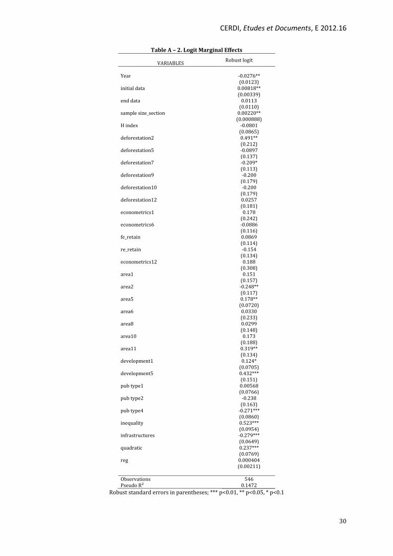
14 Tests and Logit estimations are available upon request. See Table A - 2 in the Appendix.
15 Logit and Probit estimations are available upon request to authors. Logit and Probit estimations are run on 546 observations (compared with 613 for OLS) because we have few observations for some variables.

CERDI, Etudes et Documents, E 2012.16
18
Table 4. Probit marginal effects
Robust probit
Probit cluster-robust
Probit Bootstrap cluster-robust VARIABLES
Year -0.0269** -0.0269 -0.0269*** (0.0112) (0.0176) (0.0102) initial data 0.00829*** 0.00829 0.00829*** (0.00316) (0.00531) (0.00274) end data 0.0110 0.0110 0.0110 (0.0104) (0.0164) (0.00879) sample size 0.00209** 0.00209 0.00209*** (0.000812) (0.00173) (0.000711) H index -0.0889 -0.0889 -0.0889 (0.0843) (0.180) (0.0573) deforestation2 0.486** 0.486** 0.486 (0.218) (0.200) (0.507) deforestation5 -0.0805 -0.0805 -0.0805 (0.126) (0.164) (0.114) deforestation7 -0.216* -0.216 -0.216** (0.116) (0.181) (0.105) deforestation9 -0.210 -0.210 -0.210 (0.196) (0.152) (0.137) deforestation10 -0.210 -0.210 -0.210* (0.196) (0.152) (0.127) deforestation12 0.0263 0.0263 0.0263 (0.174) (0.233) (0.155) econometrics1 0.183 0.183 0.183 (0.232) (0.277) (0.181) econometrics6 -0.0771 -0.0771 -0.0771 (0.110) (0.140) (0.108) fe_retain 0.105 0.105 0.105 (0.108) (0.122) (0.114) re_retain -0.134 -0.134 -0.134 (0.135) (0.151) (0.150) econometrics12 0.220 0.220 0.220 (0.279) (0.336) (0.201) area1 0.133 0.133 0.133 (0.143) (0.177) (0.150) area2 -0.264** -0.264 -0.264*** (0.111) (0.167) (0.0793) area5 0.166** 0.166 0.166*** (0.0678) (0.124) (0.0523) area6 0.0312 0.0312 0.0312 (0.233) (0.104) (0.209) area8 0.0259 0.0259 0.0259 (0.136) (0.178) (0.118) area10 0.156 0.156 0.156 (0.175) (0.207) (0.191) area11 0.292** 0.292* 0.292** (0.124) (0.176) (0.118) development1 0.123* 0.123 0.123** (0.0679) (0.133) (0.0573) development5 0.418** 0.418** 0.418*** (0.168) (0.172) (0.159) pub type1 0.0107 0.0107 0.0107 (0.0754) (0.134) (0.0588) pub type2 -0.221 -0.221 -0.221 (0.177) (0.194) (0.499) pub type4 -0.251*** -0.251 -0.251*** (0.0901) (0.153) (0.0802) inequality 0.530*** 0.530*** 0.530*** (0.0950) (0.133) (0.0605) infrastructures -0.297*** -0.297*** -0.297*** (0.0636) (0.106) (0.0514) quadratic 0.245*** 0.245*** 0.245*** (0.0764) (0.0827) (0.0798) reg 0.000182 0.000182 0.000182 (0.00202) (0.00275) (0.00189) Constant Observations 546 546 546 Pseudo R² 0.1478 0.1478 0.1478
Robust standard errors in parentheses; *** p<0.01, ** p<0.05, * p<0.1

CERDI, Etudes et Documents, E 2012.16
19
The quality of fit is tested. The quality of the prediction in contingency tables is
reported Table 5. The threshold is fixed at 36 % because in the population (546
observations), there are 36 % of “EKC” and 64 % of “no EKC”. Results suggest that we
reach 66.85 % of good predictions with the Probit model.
Table 5. Contingency tables Probit model for EKC
Classified D -D Total + 156 137 293 - 44 209 253
Total 200 346 546 Correctly classified : 66.85%
Classified + if predicted Pr(D) >= .36; True D defined as EKC = 0.
To validate the robustness of our results, we use other thresholds to reject the EKC,
that is to say 1% and 5% instead of 10% retained in this work. In other words, we build
two new dependent variables EKC01 and EKC05. With the first one, we choose a
significance level of 1% for the variables GDP per capita and its square. With the second
we use a threshold of 5%. Using the 10 % threshold we have 32 % of the observations
validating the EKC. It falls to 27 % for the 5 % threshold and 17 % for the 1 % one. We
then estimate the Probit model. Results do not significantly change.16
6. Results and Discussion
6.1. Main results
Our results show that the most recent year of publication is (year), the more likely to
have an EKC declines. We shall then identify the existence of non-linearity with respect
to the year of publication. In the OLS regressions (robust, cluster and bootstrap cluster),
we add the square of the year of publication. Both variables year and its square appear
to be significant in the three models, the first one having a positive coefficient and the
second having a negative one. In addition, coefficients are the same in each model
16 Tables are available from the authors upon request (See Table A – 3 in the Appendix)

CERDI, Etudes et Documents, E 2012.16
20
(respectively 18.89 and 0.00472). The turning point is around the year 2001.17,18 This
may be attributable to several factors, including an academic fad and technology
(econometric practices and better availability of data).
Empirical choices should be carefully done before deriving policies from empirical
results. On this issue, our results are not clear-cut which is not in line with (D. I. Stern
2004) contention according to which early empirical evidences of EKCs where the result
of weak econometrics.19 It is clear however from OLS regressions that the integration of
a spatial dimension (econometrics10 econometrics11) decreases the likelihood of an
EKC.20 Although these results are not to be taken per se, they raise the question of the
existence of spillovers between the rates of deforestation of countries. If these spillovers
exist, does it change the nature of the relationship between economic development and
deforestation? Existing work seem to go in that direction (e.g. Nguyen Van & Azomahou
2007).
We therefore believe that future work should incorporate the spatial dimension in
order to control for the existence of spatial autocorrelation (Anselin 1988). Regarding
deforestation, there may be several sources of spatial dependence between countries.
First, national policies for forest conservation may be influenced by policies in
neighboring countries resulting in a pattern of political spatial dependence. Second,
there may be positive or negative ecological spillovers between countries. For instance, 17 18.89/(2*0.00472) = 2001.06
18 Our robustness check provides consistent turning points. We precisely find 1999.29 for 1 %, 2000.98 for 5 % and 2000.39 for 10 %.
19 The existence of an EKC for deforestation was seldom performed on time series data. It was however the case with other types of pollutants such like CO2 or SO2. Even with recent econometric techniques, the results on the existence of an EKC are not conclusive (see e.g. Bernard et al. 2011).
20 It is likely that the number of spatial regressions is too small to be captured in Logit and Probit estimations. We run a regression with three dummies for econometric techniques: OLS, panel (dynamic, fixed effects and random effects) and spatial (panel and GWR). It did not change the results. OLS and panel estimations were not significant, whereas spatial estimations were negative and significant.

CERDI, Etudes et Documents, E 2012.16
21
seeds or forest fires – if necessary to recall – do not respect political boundaries. Third,
unobserved variables may be related by a spatial process. In the case of deforestation,
these may be climatic or geomorphological variables. And fourth, phenomena in
neighboring countries are likely to influence deforestation patterns in a given country.
For example, more stringent forest protection policies in a country may cause more
deforestation in an adjacent country. As a matter of fact, there is uncertainty about the
choice of the relevant spatial model (i.e. whether to estimate a spatial lag model, a
spatial error model, a spatial Durbin model or a Cliff-Ord type model). All effects can
occur simultaneously and there is no theoretical argument to exclude a form of spatial
dependence a priori. The use of spatial econometrics is relatively recent. Theoretical
(Corrado & Fingleton 2011; Elhorst 2010) and technical literature is growing fast
(Drukker et al. 2011). Regarding the EKC for deforestation thanks to the better
availability of data, their use will be facilitated and more relevant. This is an avenue of
research to dig that could call into question the existence of an EKC for deforestation.
At that point, we cannot conclude on the quality of data although this concern was put
forward (D. I. Stern et al. 1996).21 Still, we do find that the more recent data coincide
with the more chance of getting an EKC. It therefore stems the following question: Is it
appropriate to mix data of different quality? Our analysis cannot answer that question.
6.2. Five remarks
Sample size
The sample size (sample size) has a positive and significant effect on the existence of
the EKC. This result is line with other meta-analyses (Jeppesen et al. 2002). Indeed,
21 When gathering information we have extracted the data source. However, this information could not be used in the meta-analysis because these variables are highly correlated with measures of deforestation and because their source very often relies on FAO data.
CERDI, Etudes et Documents, E 2012.16
22
according to standard testing theory sample sizes increase the power of tests. In other
words, larger sample sizes reduce the probability of erroneously accepting the null
hypothesis.
Deforestation index
The term “deforestation” is not clear-cut. It covers a wide range of meanings. This is
striking in EKC studies for deforestation. Authors use different measures (Table 1). Our
results do not evidence a clear effect of the deforestation index on the probability of the
occurrence of an EKC for deforestation.
Infrastructures
Deforestation is driven by numerous factors. In some studies, authors only focus on
the income-deforestation nexus. In others, authors add control variables. We find that
adding infrastructures variables (infrastructures) decreases the probability of obtaining
an EKC. There is evidence that infrastructure expansion is a cause of deforestation (Pfaff
1999). However, this variable may be highly correlated to income. (D. I. Stern 2004)
addresses this issue and concludes that it is difficult to infer from studies that include
additional control variables. We add that our results for infrastructures are not
surprising. Indeed, if they are correlated with per capita income, it is normal that
authors do not find a significant relationship between economic development and
deforestation. Yet, we argue that it is not enough to conclude that there is no EKC in that
specific case, because such result could also be explained by the fact that this variable
plays a role in channelling the effect of economic development on deforestation.

CERDI, Etudes et Documents, E 2012.16
23
Inequality index
We find a strong positive relationship between the introduction of a control variable
for inequalities (inequality) and the probability of finding an EKC. Our result does not
contradict (Koop & Tole 2001) and (Heerink et al. 2001). They find that high inequality
strengthens the effect of economic development on deforestation.
Publication type
If the type of publication is a Master's thesis (pub type4), then the probability of an
EKC declines relative to an article, a working paper or conference paper, ceteris paribus.
This could be explained by a “publication strategy” effect. A Master’s student seems not
to have the same incentives to validate the existence of an EKC whereas a researcher
may be more prone to evidence an EKC as a means to publish his work in an academic
journal.
6.3. Publication Bias
Publication bias remains today the biggest problem facing meta-analyses. Indeed in
principle, the meta-analysis must combine exhaustively all the studies that have been
made in the area of interest. First there may be a bias in the reporting of results: the
estimation results are more likely to be published if they are significant. This problem is
referred as the “file drawer” problem by meta-analysts (Stanley et al. 2008). Non-
significant results may not be submitted to academic journals (nor published as a
working paper) or they may be more rejected by publishers of academic journals. Thus
the literature is not a perfect representation of all work in the field. The sources of this
type of bias are complex and highly dependent on the decisions of the authors as well as

CERDI, Etudes et Documents, E 2012.16
24
publishers. Secondly, studies with “good results” are often published in English. Here,
the means of dissemination may also be a source of publication bias.
Also, in our analysis we do not take into account the quality of the papers. This
problem is referred to as “garbage in, garbage out” (Borenstein et al. 2009). However,
we believe that excluding articles, on its own, would only add bias, compared to what we
believe to be a “good paper”. In addition, our work allows rather performing “waste
management”.22 In this sense, our work examines the characteristics of the studies that
are related to the occurrence of results.
7. Concluding Remarks
The objective of this paper was to shed light on why EKC for deforestation results
differ across studies. And that, in view of raising the attention of researchers,
practitioners and policy makers on the underlying causes that lead to the validation of
the EKC for deforestation in the academic literature, despite critical reviews of EKCs. We
have therefore constructed an original database gathering the characteristics of
econometric results for EKCs for deforestation and then implemented a meta-analysis.
Our main results are the following. Recent estimates do not corroborate the EKCs for
deforestation. The year 2001 appears to be a turning point. Our results also confirm that
empirical choices i.e. estimators choice affect the occurrence of an EKC for deforestation
with respect to the hypothesis of spatial autocorrelation in deforestation rates. The
contention of (D. I. Stern 2004) of the poor quality of econometrics underlying EKCs
estimates is thus given a particular flavour.
22 In the metaphorical sense proposed by (Borenstein et al. 2009)

CERDI, Etudes et Documents, E 2012.16
25
Finally, let us consider another interpretation of our results in a Popperian way. A
reason why EKCs are still considered is that scholars hardly make a definitive refutation
of the EKC hypothesis; they rather prefer evidencing the presence or the absence of
corrobation. Indeed, in order to test the relevance of the theory underlying the EKC,
scholars must consider auxiliary hypotheses. In the case of the EKC those auxiliary
hypotheses are partly provided by the econometric hypotheses. When the EKC is not
corroborated, scholars cannot identify whether it is the result of falsified theory or of the
econometric hypotheses. This is the essence of Quine’s holism (Quine 1951): the EKC for
deforestation cannot be tested in isolation.23 The EKC story is not at its end. Building on
our results, we can predict that empirical and theoretical research on EKCs is still lively
until theoretical alternatives will be provided. Following Popper, we can hope that
“refuted theory can be repaired to cope with the newly discovered anomalies” (Blaug
1992, p.25)
Lastly, as mentioned earlier, a meta-analysis opens the way for prospective meta-
analysis. In future work, we shall explore the quality of estimations. Indeed, in this
article we focused on estimators. Notably, we shall focus on EKC studies using panel
techniques and investigate the study-to-study variation focusing on econometric tests
performed such as tests for endogeneity, multicollinearity, Hausman test, etc.
23 The critic of Quine is also referred as the Duhem-Quine critic on the confirmation holism.

CERDI, Etudes et Documents, E 2012.16
26
References Andreoni, J. & Levinson, A., 2001. The simple analytics of the environmental Kuznets curve. Journal of
Public Economics, 80(2), p.269–286.
Angelsen, A., Brown, S., et al., 2009. Reducing Emissions from Deforestation and Forest Degradation (REDD):
an options assessment report. Prepared for the Government of Norway, Meridian Institute.
Angelsen, A., Brockhaus, M., et al. éd., 2009. Realising REDD+. National Strategy and Policy Options, Bogor: Center for International Forestry Research.
Angelsen, A. & Kaimowitz, D., 1999. Rethinking the Causes of Deforestation: Lessons from Economic Models. The World Bank Research Observer, 14(1), p.73–98.
Angrist, J.D., 2001. Estimation of Limited Dependent Variable Models with Dummy Endogenous Regressors: Simple Strategies for Empirical Practice. Journal of Business & Economic Statistics, 19(1), p.2–16.
Anselin, L., 1988. Spatial econometrics: methods and models, Dordrecht: Kluwer Academic Publishers.
Arrow, K. et al., 1996. Economic Growth, Carrying Capacity, and the Environment. Environment and
Development Economics, 1(01), p.104–110.
Barbier, E.B., 2001. The Economics of Tropical Deforestation and Land Use: An Introduction to the Special Issue. Land Economics, 77(2), p.155–171.
Barbier, E.B., Burgess, J.C. & Grainger, A., 2010. The forest transition: Towards a more comprehensive theoretical framework. Land Use Policy, 27(2), p.98–107.
Barrio, M. & Loureiro, M.L., 2010. A meta-analysis of contingent valuation forest studies. Ecological
Economics, 69(5), p.1023–1030.
Beckerman, W., 1992. Economic growth and the environment: Whose growth? whose environment? World
Development, 20(4), p.481–496.
Bernard, J.-T. et al., 2011. The Environmental Kuznets Curve: Tipping Points, Uncertainty and Weak Identification. SSRN eLibrary. Available at: http://papers.ssrn.com/sol3/papers.cfm?abstract_id=1974622.
Blaug, M., 1992. The Methodology of Economics. Or, How Economists Explain 2nd ed., Cambridge University Press.
Borenstein, M. et al., 2009. Introduction to Meta-Analysis, Chichester UK: John Wiley and Sons.
Carson, R.T., 2010. The Environmental Kuznets Curve: Seeking Empirical Regularity and Theoretical Structure. Review of Environmental Economics and Policy, 4(1), p.3 –23.
Cavlovic, T.A. et al., 2000. A meta-analysis of environmental Kuznets curve studies. Agricultural and
Resource Economics Review, 29(1), p.32–42.
Chatterjee, S. & Hadi, A.S., 2006. Regression Analysis by Example 4th ed., John Wiley and Sons.
Corrado, L. & Fingleton, B., 2011. Where Is the Economics in Spatial Econometrics? Journal of Regional
Science, p.1–30.
Dinda, S., 2004. Environmental Kuznets Curve Hypothesis: A Survey. Ecological Economics, 49(4), p.431–455.
Drukker, D.M., Prucha, I.R. & Raciborski, R., 2011. A command for estimating spatial-autoregressive models with spatial-autoregressive disturbances and additional endogenous variables. The Stata
Journal, 1(1), p.1–13.
Elhorst, J.P., 2010. Applied Spatial Econometrics: Raising the Bar. Spatial Economic Analysis, 5(1), p.9–28.
Engel, S. & Palmer, C., 2008. « Painting the forest REDD? » Prospects for mitigating climate change through reducing emissions from deforestation and degradation. IED Working paper, (3).
Geist, H.J. & Lambin, E.F., 2001. What drives tropical deforestation? A meta-analysis of proximate and
underlying causes of deforestation based on subnational case study evidence, Louvain-la-Neuve: LUCC International Project Office - University of Louvain.

CERDI, Etudes et Documents, E 2012.16
27
Grossman, G.M. & Krueger, A.B., 1995. Economic Growth and the Environment. The Quarterly Journal of
Economics, 110(2), p.353–377.
Heerink, N., Mulatu, A. & Bulte, E., 2001. Income inequality and the environment: aggregation bias in environmental Kuznets curves. Ecological Economics, 38(3), p.359–367.
Hunter, J.E. & Schmidt, F.L., 2004. Methods of Meta-Analysis. Correcting Errors and Bias in Research
Findings, Sage.
Jacobsen, J.B. & Hanley, N., 2008. Are There Income Effects on Global Willingness to Pay for Biodiversity Conservation? Environmental and Resource Economics, 43(2), p.137–160.
Jeppesen, T., List, J.A. & Folmer, H., 2002. Environmental Regulations and New Plant Location Decisions: Evidence from a Meta‐Analysis. Journal of Regional Science, 42(1), p.19–49.
Jordan, B.R., 2010. The Environmental Kuznets Curve: Preliminary Meta-Analysis of Published Studies, 1995-2010. Dans Workshop on Original Policy Research. Georgia Tech - School of Public Policy.
Kiel, K.A. & Williams, M., 2007. The impact of Superfund sites on local property values: Are all sites the same? Journal of Urban Economics, 61(1), p.170–192.
Koop, G. & Tole, L., 2001. Deforestation, distribution and development. Global Environmental Change, 11(3), p.193–202.
Koop, G. & Tole, L., 1999. Is there an environmental Kuznets curve for deforestation? Journal of
Development Economics, 58(1), p.231–244.
Kuhn, T.S., 1996. The structure of scientific revolutions 3rd ed., Chicago: University of Chicago Press.
Levinson, A., 2002. The ups and downs of the environmental Kuznets curve. In J. A. List & A. de Zeeuw, ed. Recent advances in environmental economics. London: Edward Elgar, p. 119.
Lindhjem, H., 2007. 20 years of stated preference valuation of non-timber benefits from Fennoscandian forests: A meta-analysis. Journal of Forest Economics, 12(4), p.251–277.
Ma, C. & Stern, D.I., 2006. Environmental and ecological economics: A citation analysis. Ecological
Economics, 58(3), p.491–506.
Mariani, F., Pérez-Barahona, A. & Raffin, N., 2010. Life expectancy and the environment. Journal of
Economic Dynamics and Control, 34(4), p.798–815.
Mather, A.S., 1992. The Forest Transition. Area, 24(4), p.367–379.
Mather, A.S., Needle, C.L. & Fairbairn, J., 1999. Environmental Kuznets Curves and Forest Trends. Geography, 84(1), p.55–65.
McCloskey, D.N., 1983. The Rhetoric of Economics. Journal of Economic Literature, 21(2), p.481–517.
Munasinghe, M., 1999. Is environmental degradation an inevitable consequence of economic growth: tunneling through the environmental Kuznets curve. Ecological Economics, 29(1), p.89–109.
Nelson, J.P. & Kennedy, P.E., 2008. The Use (and Abuse) of Meta-Analysis in Environmental and Natural Resource Economics: An Assessment. Environmental and Resource Economics, 42(3), p.345–377.
Nguyen Van, P. & Azomahou, T., 2007. Nonlinearities and heterogeneity in environmental quality: An empirical analysis of deforestation. Journal of Development Economics, 84(1), p.291–309.
Panayotou, T., 1993. Empirical Tests and Policy Analysis of environmental Degradation at Different Stages of
Economic Development, Geneva: International Labor Office.
Pfaff, A.S.P., 1999. What Drives Deforestation in the Brazilian Amazon?: Evidence from Satellite and Socioeconomic Data. Journal of Environmental Economics and Management, 37(1), p.26–43.
Quine, W.V.O., 1951. Main Trends in Recent Philosophy: Two Dogmas of Empiricism. The Philosophical
Review, 60(1), p.20–43.
Roy Chowdhury, R. & Moran, E.F., 2012. Turning the curve: A critical review of Kuznets approaches. Applied Geography, 32(1), p.3–11.
Rudel, T.K. et al., 2005. Forest transitions: towards a global understanding of land use change. Global
Environmental Change, 15(1), p.23–31.

CERDI, Etudes et Documents, E 2012.16
28
Rudel, T.K. & Roper, J., 1997. The paths to rain forest destruction: Crossnational patterns of tropical deforestation, 1975-1990. World Development, 25(1), p.53–65.
Schläpfer, F., 2006. Survey protocol and income effects in the contingent valuation of public goods: A meta-analysis. Ecological Economics, 57(3), p.415–429.
Shafik, N. & Bandyopadhyay, S., 1992. Economic Growth and Environmental Quality. Time-Series and Cross-Country Evidence. Policy Research Working Papers Series, 904.
Stanley, T.D., 2001. Wheat from Chaff: Meta-Analysis as Quantitative Literature Review. The Journal of
Economic Perspectives, 15(3), p.131–150.
Stanley, T.D., Doucouliagos, C. & Jarrell, S.B., 2008. Meta-regression analysis as the socio-economics of economics research. Journal of Socio-Economics, 37(1), p.276–292.
Stern, D.I., 2004. The Rise and Fall of the Environmental Kuznets Curve. World Development, 32(8), p.1419–1439.
Stern, D.I., Common, M.S. & Barbier, E.B., 1996. Economic growth and environmental degradation: The environmental Kuznets curve and sustainable development. World Development, 24(7), p.1151–1160.
Stern, N.H., 2007. The economics of climate change: the Stern review, Cambridge University Press.
Xepapadeas, A., 2005. Chapter 23 Economic growth and the environment. Dans K.-G. Mäler & J. R. Vincent, éd. Economywide and International Environmental Issues. Elsevier, p. 1219–1271.

CERDI, Etudes et Documents, E 2012.16
29
Appendix A – For the referees, not for publication
Table A – 1. Studies included in the sample (authors, year of publication, support of the publication)
Antle & Heidebrink (1995) Economic Development and
Cultural Change
Araujo et al (2009) Ecological Economics
Arcand et al (2008) Journal of Development Economics
Arcand et al (2002) CERDI working papers
Barbeau (2003) University de Montreal, Départment de
sciences économiques, Rapport de recherche
Barbier (2004) American Journal of Agricultural
Economics
Barbier & Burgess (2001) Journal of Economic Surveys
Basu & Nayak (2011) Forest Policy and Economics
Bhattarai & Hammig (2004) Environment and
Development Economics
Bhattarai & Hammig (2001) World Development
Castro Gomes & José Braga (2008) Universidade
Federal De Viçosa-UFV, Working papers
Buitenzorgy & Mol (2011) Environmental and Resource
Economics
Caviglia-Harris et al (2009) Ecological Economics
Combes et al (2008) CERDI working papers
Combes et al (2010) CERDI working papers
Combes Motel et al (2009) Ecological Economics
Corderi (2008) Economic Analysis Working Papers,
Colexio de Economistas de A Coruña, Spain and
Fundación Una Galicia Moderna
Cornelis van Kooten & Wang (2003) XII World Forestry
Congress (FAO)
Corrêa de Oliveira & Simoes de Almeida (2011)
Department of Economics- Federal University of Juiz
Juiz de Fora
Cropper & Griffiths (1994) American Economic Review
Culas & Dutta (2003) Working papers, University of
Sydney, Department of economics
Culas (2007) Ecological Economics
Damette & Delacote (2011) Ecological Economics
Delacote (2003) Mémoire de DEA CERDI
Diarra & Marchand (2011) CERDI working papers
Diarrasouba & Boubacar (2009) Selected paper for
presentation at the southern Agricultural economics
Association Annual Meeting
Duval & Wolff (2009) Laboratoire d'Economie et de
Management Nantes-Atlantique Université de Nantes,
HAL working Papers
Ehrhardt-Martinez et al (2002) Social Science Quarterly
Ehrhardt-Martinez (1998) Social Forces
Ferreira (2004) Land Economics
Frankel & Rose (2002) NBER Working papers
Galinato & Galinato (2010) Working papers, School of
Economic Sciences, Washington State University
Gangadharan & Valenzuela (2001) Ecological
Economics
Heerink et al (2001) Ecological Economics
Hilali & Ben Zina (2007) Unité de Recherches sur la
Dynamique Economique et l'Environnement (URDEE)
Hyde et al (2008) Environment for Development
Jorgenson (2006) Rural Sociology
Jorgenson (2008) The Sociological Quarterly
Kahuthu (2006) Environment, Development and
Sustainability
Kallbekken (2000) Environmental Economics and
Environmental Management, University of York
Kishor & Belle (2004) Journal of Sustainable Forestry
Koop & Tole (1999) Journal of Development Economics
Lantz (2002) Journal of Forest Economics
Lee et al (2009) Singapore Economic review conference
Leplay & Thoyer (2011) Laboratoire d'Economie et de
Management Nantes-Atlantique Université de Nantes,
HAL working Papers
Li (2006) International Studies Quarterly
Lim (1997) School of economics, University of New
South Wales Sydney, NSW 2no52, Australia
Lopez & Galinato (2004) Environmental Protection
Agency (EPA) report
Marchand (2010) CERDI working papers
Marquart-Pyatt (2004) International Journal of Sociology
Meyer et al (2003) International Forestry Review
Naito & Traesupap (2006) Journal of The faculty of
Economics, KGU
Nguyen Van & Azomahou (2003) Revue Economique
Nguyen Van & Azomahou (2007) Journal of
Development Economics
Panayotou (1993) World Employment Programme
research Working papers
Perrings & Ansuategi (2000) Journal of Economic
Studies
Reuveny et al (2010) Journal of Peace Research
Rock (1996) Ecological Economics
Shafik (1994) Oxford Economic Papers
Shafik & Bandyopadhyay (1992) Policy Research
Working papers, World Bank
Shandra (2007) Sociological Inquiry
Shandra (2007) International Journal of Comparative
Sociology
Shandra (2007) Social Science Quarterly
Skonhoft & Solem (2001) Ecological Economics
Turner et al (2006) Scandinavian Journal of Forest
Research
Turner et al (2005) Agricultural and Resource Economics
Review
Wang et al (2007) Forest Policy and Economics
Wang (2003) XII World Forestry Congress 2nono3
(FAO)
Yoshioka (2010) Faculty of economics, Nagasaki
University
Zhao et al (2011) Environment and Resource Economics
Zhu & Zhang (2006) Journal of Agricultural and Applied
Economics
CERDI, Etudes et Documents, E 2012.16
30
Table A – 2. Logit Marginal Effects
Robust logit VARIABLES
Year -0.0276** (0.0123) initial data 0.00818** (0.00339) end data 0.0113 (0.0110) sample size_section 0.00220** (0.000888) H index -0.0801 (0.0865) deforestation2 0.491** (0.212) deforestation5 -0.0897 (0.137) deforestation7 -0.209* (0.113) deforestation9 -0.200 (0.179) deforestation10 -0.200 (0.179) deforestation12 0.0257 (0.181) econometrics1 0.178 (0.242) econometrics6 -0.0886 (0.116) fe_retain 0.0869 (0.114) re_retain -0.154 (0.134) econometrics12 0.188 (0.308) area1 0.151 (0.157) area2 -0.248** (0.117) area5 0.178** (0.0720) area6 0.0330 (0.233) area8 0.0299 (0.148) area10 0.173 (0.188) area11 0.319** (0.134) development1 0.124* (0.0705) development5 0.432*** (0.151) pub type1 0.00568 (0.0766) pub type2 -0.238 (0.163) pub type4 -0.271*** (0.0860) inequality 0.523*** (0.0954) infrastructures -0.279*** (0.0649) quadratic 0.237*** (0.0769) reg 0.000404 (0.00211)
Observations 546 Pseudo R² 0.1472
Robust standard errors in parentheses; *** p<0.01, ** p<0.05, * p<0.1

CERDI, Etudes et Documents, E 2012.16
31
Table A - 3. Probit robustness check VARIABLES EKC01 EKC05
Year -0.0936*** -0.0630**
(0.0361) (0.0320)
initial data 0.0378*** 0.0195**
(0.0118) (0.00865)
end data 0.0104 0.0111
(0.0382) (0.0321)
sample size 0.00556* 0.00472**
(0.00319) (0.00211)
H index -0.175 -0.0494
(0.301) (0.254)
deforestation2 4.822*** 0.710
(0.736) (0.934)
deforestation5 -1.314*** -0.886**
(0.405) (0.355)
deforestation7 -2.194*** -1.577***
(0.698) (0.486)
deforestation9 -1.019 -0.933
(0.830) (0.811)
deforestation10 -1.019 -0.933
(0.830) (0.811)
deforestation11 -1.009 0.686
(0.925) (0.898)
deforestation12 -0.699
(0.576)
econometrics1 0.249 0.483
(0.661) (0.613)
econometrics6 -0.559 0.0765
(0.402) (0.322)
fe_retain -0.125 0.278
(0.366) (0.314)
re_retain -0.798 -0.497
(0.674) (0.500)
econometrics12 1.743** 1.101
(0.760) (0.737)
area1 0.261 0.225
(0.486) (0.375)
area2 -0.894 -0.916
(0.655) (0.587)
area5 0.469** 0.456***
(0.208) (0.175)
area6 -0.385
(0.606)
area8 0.168 -0.151
(0.479) (0.411)
area10 0.0680
(0.451)
area11 -0.0783 0.565*
(0.490) (0.334)
development1 0.852*** 0.389**
(0.224) (0.195)
development5 0.922 1.356**
(0.683) (0.605)
pub type1 0.269 0.0305
(0.269) (0.215)
pub type2 -4.576*** -0.273
(0.355) (0.768)
pub type4 -1.598*** -1.170***
(0.487) (0.386)
inequality 1.527*** 0.789*
(0.432) (0.428)
infrastructures -12.35 -5.542***
(8.348) (1.912)
quadratic 0.771** 0.828**
(0.392) (0.347)
reg 0.0169** 0.0101*
(0.00686) (0.00600)
Constant 90.88** 64.09**
(36.65) (31.70)
Observations 512 550
Pseudo R² 0.2908 0.1873
Robust standard errors in parentheses; *** p<0.01, ** p<0.05, * p<0.1
Top Related