


Languages
Pages
Legal


The Design and Implementation of a
Simulator for Multistatic RadarSystems
Marc BrookerBSc (Eng) UCT
A thesis submitted to the Department of Electrical Engineering,University of Cape Town, in fulfilment of the requirements for
the degree of
Doctor of Philosophy
at the
University of Cape Town
June 2008

“The purpose of computing is insight, not numbers.”Richard W. Hamming
i

Declaration
This report and the project on which it is based is entirely my own
work.
I have used the IEEE convention for citation and referencing. Each contri-
bution to, and quotation in, this report from the works of others has been
attributed, cited and referenced.
I have not allowed, nor will allow, any other student to copy my work with
the intention of passing it off as their own.
I acknowledge that plagiarism is wrong, and declare that this report, and the
project on which it is based, is entirely my own work.
Marc Brooker
ii

Abstract
This thesis presents the design and implementation of a signal level simulator
supporting a wide variety of radar systems, and focusing on multistatic and
netted radars. The simulator places few limits on the simulated system,
and supports systems with arbitrary numbers of receivers, transmitters,
and scatterers. Similarly, the simulator places no restrictions on the radar
waveform to be simulated, and supports pulsed, continuous wave (CW) and
carrier-free radar systems.
A flexible model is used to describe the radar system to be simulated, with
the parameters of the radar hardware, the properties of scatterers and the
layout of objects in the simulated environment specified in XML format. The
development of the simulation model focused on balancing the requirements
of flexibility and usability, ensuring that the model can be efficiently used to
represent any type of radar system.
Oscillator phase noise is a limiting factor on the performance of some
types of radar systems. The development of a model for the deterministic
and static components of phase noise is presented. Based on this model,
an algorithm for the efficient generation of synthetic phase noise sequences
was developed, based on a multirate signal processing approach. This thesis
presents this algorithm, and results of simulations of the effects of phase noise
on synthetic aperture radar (SAR) and pulse-Doppler radar systems.
The FERS simulator, an implementation of the simulation model presented
in this thesis, was developed in the C++ and Python programming languages.
This simulator is able to perform real-time simulation of some common radar
configurations on commodity PC hardware, taking advantage of multicore and
multiprocessor machines. FERS has been released as open source software
iii

under the GNU general public licence (GPL).
Validation of the simulator output was performed by comparison of simu-
lation results with both theory and measurements. The simulator output was
found to be accurate for a wide variety of radar systems, including netted
pulse-Doppler, moving target indication (MTI) and synthetic aperture (SAR)
radar systems.
iv

Acknowledgements
I am extremely grateful for the advice and guidance of my supervisor, Professor
Michael Inggs. Through sharing his expertise and extensive insight into
the theory and practice of radar, Professor Inggs has earned my highest
appreciation and made working on this project a extraordinarily fulfilling
experience.
This work would not have been possible without the financial support of
the SANDF, and the assistance of the CSIR Ledger program.
I would also like to thank the members of the Radar Remote Sensing
Group (RRSG) for providing me with a stimulating and enjoyable research
environment; Shaun Doughty, Stephan Sandenbergh and Sebastiaan Heunis
for sharing some of the data that was used for the validation of FERS; and
Regine Lord for protecting me from the university administration system. I
am grateful for the advice provided to me by Professor Christopher Baker
and Karl Woodbridge from University College London.
My parents, Chris and Elaine Brooker, have been especially supportive
and patient.
Finally, I would like to thank Kate McWilliams for providing me with
assistance, support, and inspiration.
v

Contents
Declaration ii
Abstract iii
Acknowledgements v
List of Figures ix
List of Tables xiii
List of Algorithms xiv
Nomenclature xv
1 Introduction 1
1.1 Research Objectives . . . . . . . . . . . . . . . . . . . . . . . . 1
1.2 Significance of Research . . . . . . . . . . . . . . . . . . . . . 8
1.3 Structure of Thesis . . . . . . . . . . . . . . . . . . . . . . . . 9
1.4 Statement of Originality . . . . . . . . . . . . . . . . . . . . . 10
2 Discrete-Time Radar Simulation Model 12
2.1 Introduction . . . . . . . . . . . . . . . . . . . . . . . . . . . . 12
2.2 Environment Model . . . . . . . . . . . . . . . . . . . . . . . . 21
2.3 Hardware Model . . . . . . . . . . . . . . . . . . . . . . . . . 37
2.4 Conclusion . . . . . . . . . . . . . . . . . . . . . . . . . . . . . 42
vi

CONTENTS
3 Time and Frequency Simulation 43
3.1 Introduction . . . . . . . . . . . . . . . . . . . . . . . . . . . . 43
3.2 Stochastic Model of Frequency Sources . . . . . . . . . . . . . 45
3.3 Generation of Synthetic Phase Noise Sequences . . . . . . . . 55
3.4 Multirate Filters and Noise Generation . . . . . . . . . . . . . 61
3.5 Phase Noise Generation Using Multirate Filters . . . . . . . . 69
3.6 Efficient Noise Synthesis for Pulsed Radar . . . . . . . . . . . 73
3.7 Effects of Oscillator Behaviour On Radar Signals . . . . . . . 77
3.8 Conclusion . . . . . . . . . . . . . . . . . . . . . . . . . . . . . 80
4 Simulator Development 81
4.1 Introduction . . . . . . . . . . . . . . . . . . . . . . . . . . . . 81
4.2 Software Structure and Implementation . . . . . . . . . . . . . 84
4.3 Fractional Delay Filter Design . . . . . . . . . . . . . . . . . . 97
4.4 Conclusion . . . . . . . . . . . . . . . . . . . . . . . . . . . . . 104
5 Validation of Simulator Accuracy 106
5.1 Introduction . . . . . . . . . . . . . . . . . . . . . . . . . . . . 106
5.2 Comparison with Theoretical Predictions . . . . . . . . . . . . 107
5.3 Comparison with Measurements . . . . . . . . . . . . . . . . . 117
5.4 Simulation of Phase Noise Effects . . . . . . . . . . . . . . . . 123
5.5 Conclusion . . . . . . . . . . . . . . . . . . . . . . . . . . . . . 125
6 Conclusion 126
6.1 Summary and Contributions . . . . . . . . . . . . . . . . . . . 126
6.2 Future Work . . . . . . . . . . . . . . . . . . . . . . . . . . . . 129
A Stochastic Simulation 132
A.1 Introduction . . . . . . . . . . . . . . . . . . . . . . . . . . . . 132
A.2 Bistatic Pulse-Doppler Radar . . . . . . . . . . . . . . . . . . 133
A.3 Synthetic Aperture Radar (SAR) . . . . . . . . . . . . . . . . 137
A.4 Conclusion . . . . . . . . . . . . . . . . . . . . . . . . . . . . . 143
vii

CONTENTS
B Limitations of the Simulation Model 144
B.1 Introduction . . . . . . . . . . . . . . . . . . . . . . . . . . . . 144
B.2 Linearity . . . . . . . . . . . . . . . . . . . . . . . . . . . . . . 144
B.3 Multiscatter . . . . . . . . . . . . . . . . . . . . . . . . . . . . 146
References 149
viii

List of Figures
1.1 Simulated SAR image of E-3 sentry aircraft, created by SARviz
(from [1]) . . . . . . . . . . . . . . . . . . . . . . . . . . . . . 3
1.2 Result viewer from SARSIM II showing the raw signal results
of simulation (from [2]) . . . . . . . . . . . . . . . . . . . . . . 4
1.3 Six widely used radar configurations, illustrating the diversity
of radar systems — and the common elements present in every
configuration. . . . . . . . . . . . . . . . . . . . . . . . . . . . 7
2.1 Bistatic passive receiver system . . . . . . . . . . . . . . . . . 14
2.2 Bistatic radar system showing possible propagation paths. . . 15
2.3 Comparison of real valued lowpass and bandpass radar signals. 16
2.4 Magnitude of the Fourier transform of the complex envelope
of the signal x(t) . . . . . . . . . . . . . . . . . . . . . . . . . 17
2.5 Axes of the model coordinate system . . . . . . . . . . . . . . 20
2.6 Transmission paths for transmitted energy from transmitter to
receiver. . . . . . . . . . . . . . . . . . . . . . . . . . . . . . . 21
2.7 Heirarchy of objects in the object model . . . . . . . . . . . . 23
2.8 Block diagram of the effect of phase shift on quadrature recep-
tion. Upmixers include suitable low pass filters. . . . . . . . . 25
2.9 Cumulative density functions and probability density functions
for Swerling cases 1 and 3 (σ = 1) . . . . . . . . . . . . . . . . 28
2.10 Geometric arrangement for reflection approach to multipath
simulation . . . . . . . . . . . . . . . . . . . . . . . . . . . . . 33
2.11 Equivalence of rearrangement of system geometry and multi-
path propagation . . . . . . . . . . . . . . . . . . . . . . . . . 35
ix
LIST OF FIGURES
2.12 Block diagram of the transmitter hardware model . . . . . . . 38
2.13 Block diagram of the receiver hardware model . . . . . . . . . 41
3.1 Doppler radar sensitivity is limited by clock phase noise where
clutter spreading exceeds the system thermal noise floor. Adapted
from Leeson et. al. [3] . . . . . . . . . . . . . . . . . . . . . . 43
3.2 Doppler shift of common target types versus system frequency.
Adapted from Vig [4] . . . . . . . . . . . . . . . . . . . . . . . 44
3.3 Comparison of specified phase noise measurements from two
quartz oscillators . . . . . . . . . . . . . . . . . . . . . . . . . 48
3.4 Examples of categories of phase noise, corresponding to power
law spectra of Sx(f) . . . . . . . . . . . . . . . . . . . . . . . 49
3.5 Definition of Period Jitter and Time Interval Error (after [5]) . 54
3.6 Deviation of truncated filters from the target response for
N = 105 and α = 1 (from [6]) . . . . . . . . . . . . . . . . . . 58
3.7 Comparison of deviations from the exact response of an optimal
IIR filter, and an AR filter designed using equation 3.30 (from
[6]) . . . . . . . . . . . . . . . . . . . . . . . . . . . . . . . . . 59
3.8 Comparison of deviation from α = 1 response for least-squares
optimal filter and truncated ideal filter (order = 30) . . . . . . 60
3.9 Deviation from α = 1 response for least-squares optimal filter
over the top decade of frequency (order = 10) . . . . . . . . . 63
3.10 Filter structure for Y (ω) . . . . . . . . . . . . . . . . . . . . . 64
3.11 Simple multirate implementation of filter structure for Y (ω) . 64
3.12 Optimised multirate implementation of filter structure for Y (ω)
(Adapted from Park et. al. [7]) . . . . . . . . . . . . . . . . . 65
3.13 A single branch of the optimised multirate filter structure for
Y (ω) . . . . . . . . . . . . . . . . . . . . . . . . . . . . . . . . 66
3.14 Comparison of generated noise PSD versus required PSD for
two coloured pseudonoise sequences . . . . . . . . . . . . . . . 68
3.15 Piecewise linear representation of the power law noise model . 69
x

LIST OF FIGURES
3.16 Modified multirate filter structure for the efficient generation
of noise matching a spectrum polynomial in f−1 (from Brooker
et. al. [6]) . . . . . . . . . . . . . . . . . . . . . . . . . . . . . 71
3.17 Results of synthesis of phase noise matching the specifications
of the Maxim DS4026 10MHz TCXO [8] . . . . . . . . . . . . 72
3.18 Autocorrelation of filtered noise sequences for α = 0 . . . . . . 74
3.19 Amplitude error as a result of ADC timing jitter (after [9]) . . 78
3.20 Data converter maximum SNR versus RMS timing jitter . . . 79
4.1 Block diagram of simulator software structure and data flow . 84
4.2 Bitmap antenna view and corresponding 3D gain plot . . . . . 86
4.3 Bistatic RCS (in dBm2) of an F5 fighter for transmitter at
(-60, 60) (data courtesy of Professor Keith Palmer, University
of Stellenbosch) . . . . . . . . . . . . . . . . . . . . . . . . . . 87
4.4 Simulator performance in return samples per second versus
transmitted pulse length and target count . . . . . . . . . . . 93
4.5 Simulator performance in return samples per second versus
transmitted pulse length . . . . . . . . . . . . . . . . . . . . . 94
4.6 Simulation time reduction versus pulse length for a four core
SMP computer . . . . . . . . . . . . . . . . . . . . . . . . . . 95
4.7 The effect of Kaiser window β parameter on the frequency
response of a FIR fractional delay filter with N = 32 . . . . . 100
4.8 The effect of filter length on the frequency response of a FIR
fractional delay filter (β = 5) . . . . . . . . . . . . . . . . . . . 101
4.9 Error of polynomial approximation of Kaiser window function
(N = 32, β = 5) . . . . . . . . . . . . . . . . . . . . . . . . . . 103
4.10 Peak subsample delay error versus distance from filter table
entry . . . . . . . . . . . . . . . . . . . . . . . . . . . . . . . . 104
5.1 Comparison simulated MTI improvement versus theoretically
predicted limit . . . . . . . . . . . . . . . . . . . . . . . . . . . 109
5.2 MTI Improvement factor limitation due to antenna scan mod-
ulation . . . . . . . . . . . . . . . . . . . . . . . . . . . . . . . 110
5.3 Airborne Stripmap SAR Geometry . . . . . . . . . . . . . . . 111
xi

LIST OF FIGURES
5.4 Processed results of VHF SAR simulation with single target . 112
5.5 Processed results of VHF SAR simulation with multiple targets113
5.6 The effect of synthetic aperture length on the sharpness of
SAR targets . . . . . . . . . . . . . . . . . . . . . . . . . . . . 113
5.7 Effect of sensor trajectory deviations on SAR processing . . . 114
5.8 Layout of the transmitter, receiver and target for PCL simulations115
5.9 Range-Doppler plots for processed PCL simulation results
(simulation by Sebastiaan Heunis) . . . . . . . . . . . . . . . . 116
5.10 Netrad geometry used for validation measurements . . . . . . 118
5.11 Measured and simulated range-Doppler images for netted radar
experiment . . . . . . . . . . . . . . . . . . . . . . . . . . . . . 120
5.12 Cuts through netted radar measurement and simulation in
range and Doppler . . . . . . . . . . . . . . . . . . . . . . . . 121
5.13 Experimental setup for CW sonar system . . . . . . . . . . . . 122
5.14 Comparison of measured and simulated results for pendulum
experiment . . . . . . . . . . . . . . . . . . . . . . . . . . . . . 124
A.1 Measured phase noise of NetRad cable-based clock transfer
system, and polynomial fit . . . . . . . . . . . . . . . . . . . . 134
A.2 Direct signal power spreading in range and Doppler versus
integration time for measured NetRad phase noise . . . . . . . 135
A.3 Direct signal power spreading in range and Doppler bins . . . 136
A.4 Cross sections of a single point in a SAR image . . . . . . . . 139
A.5 Histogram of distribution of ISLR for noise amplitude−40dBc/Hz
and α = 0 (100 experiments) . . . . . . . . . . . . . . . . . . . 142
B.1 Geometry of multiscatter example . . . . . . . . . . . . . . . . 148
xii

List of Tables
2.1 Jones vectors corresponding to various polarization cases . . . 20
2.2 Relation of chi-square fluctuations to other commonly used
fluctuation models . . . . . . . . . . . . . . . . . . . . . . . . 29
2.3 Parameters of the point target model . . . . . . . . . . . . . . 31
2.4 Parameters of multipath simulation surface . . . . . . . . . . . 37
2.5 Parameters of the transmitter hardware model . . . . . . . . . 40
2.6 Parameters of the receiver hardware model . . . . . . . . . . . 41
5.1 SASAR System Parameters (after [10]) . . . . . . . . . . . . . 111
A.1 Mean integrated sidelobe ratios (dB) versus noise amplitude
and category (α) . . . . . . . . . . . . . . . . . . . . . . . . . 141
A.2 Standard deviation of integrated sidelobe ratios (dB) versus
noise amplitude and category (α) . . . . . . . . . . . . . . . . 142
xiii

List of Algorithms
1 Dynamic pruning algorithm . . . . . . . . . . . . . . . . . . . 75
2 World model flow . . . . . . . . . . . . . . . . . . . . . . . . . 88
3 World model controller flow . . . . . . . . . . . . . . . . . . . 89
4 Environment model flow . . . . . . . . . . . . . . . . . . . . . 89
5 Thread controller flow . . . . . . . . . . . . . . . . . . . . . . 91
6 Response renderer flow . . . . . . . . . . . . . . . . . . . . . . 91
7 Window renderer flow . . . . . . . . . . . . . . . . . . . . . . 92
xiv

Nomenclature
ADC Analogue to Digital Converter
AR Autoregressive
ARMA Autoregressive Moving Average
CW Continuous Wave
DAC Digital to Analogue Converter
DDS Direct Digital Synthesis
EW Electronic Warfare
FIR Finite Impulse Response
FM Frequency Modulation
GUI Graphical User Interface
IIR Infinite Impulse Response
ISLR Integrated Sidelobe Ratio
ISO International Organization for Standardization
LF Low Frequency
LNA Low Noise Amplifier
MTI Moving Target Indication
xv

LIST OF ALGORITHMS
OCXO Oven Controlled Crystal Oscillator
PCL Passive Coherent Location
PCM Pulse Code Modulation
PM Phase Modulation
PRF Pulse Repetition Frequency
PRI Pulse Repetition Interval
PSD Power Spectral Density
PSL Peak Sidelobe Level
PSM Polarization Scattering Matrix
RCS Radar Cross Section
RF Radio Frequency
RRSG Radar Remote Sensing Group
SAR Synthetic Aperture Radar
SMP Symmetric Multiprocessing
STFT Short Time Fourier Transform
STP Standard Temperature and Pressure
T-R Transmit-Receive
TCXO Temperature Compensated Crystal Oscillator
TIE Time Interval Error
UCT University of Cape Town (South Africa)
xvi

Chapter 1
Introduction
1.1 Research Objectives
This thesis presents the development and validation of a simulator for netted
and multistatic [11] radar systems. The key objectives of this research were
to:
• Research and develop algorithms for the signal level simulation of
radar systems. The algorithms required must support the simulation of
systems with arbitrary numbers of receivers, transmitters and targets.
Simulation algorithms must also efficiently support CW radar, wideband
and carrier-free radar systems.
• Research and develop algorithms for the simulation of the effects of
phase noise and jitter on radar systems, and the synthesis of phase noise
matching measured oscillator parameters.
• Develop a complete simulator using the algorithms for radar simulation
and clock simulation. Key requirements for the simulator include
portability, ease of use, and applicability to a wide variety of radar
simulation problems.
• Verify that the simulation results are accurate, within the bounds of
the limitations of the simulation algorithms. Comparisons with both
1

1.1. RESEARCH OBJECTIVES
measured data and theoretical expectations must be performed, and
the differences between simulation results and expect results explained.
• Use the simulator to predict emergent behaviours not explicitly included
in the simulation model.
• Demonstrate that large multistatic radar systems can be simulated, at
the signal level, using low-cost computer hardware.
These objectives were identified as supporting the goal of developing
an accurate and flexible signal level simulator for monostatic, multistatic
and netted radar systems without restrictions on geometry, system design,
bandwidth or any other key parameter. The key hypothesis of this work is
that it is possible, with commodity computing hardware, to simulate the
performance of radar systems at the signal level with no restrictions on the
parameters of the systems to be simulated.
1.1.1 Radar Simulation
Radar simulators can be divided into a number of categories depending on
the type of results they are intended the produce, and the expectations of
the end user. Broadly defined, the categories of radar simulators are:
Result simulators produce a simulation of the results, after processing,
which could be expected when a radar system is run in a particular
environment. These types of simulators are useful for training both
humans and machines in result interpretation, training humans on radar
system operation, and simulating the effects of radar countermeasures
and camouflage. These types of simulators can run extremely efficiently,
as they do not need to model the actual operation of a radar system —
only the expected results.
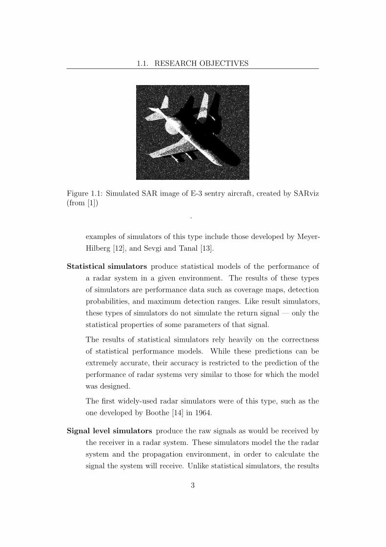
Figure 1.1 illustrates the results of the SAR image simulator, SARviz,
developed by Balz, et. al. [1] The simulator has produced a simulation
of how an E-3 Sentry aircraft would appear to a SAR system. Other
2
1.1. RESEARCH OBJECTIVES
Figure 1.1: Simulated SAR image of E-3 sentry aircraft, created by SARviz(from [1])
.
examples of simulators of this type include those developed by Meyer-
Hilberg [12], and Sevgi and Tanal [13].
Statistical simulators produce statistical models of the performance of
a radar system in a given environment. The results of these types
of simulators are performance data such as coverage maps, detection
probabilities, and maximum detection ranges. Like result simulators,
these types of simulators do not simulate the return signal — only the
statistical properties of some parameters of that signal.
The results of statistical simulators rely heavily on the correctness
of statistical performance models. While these predictions can be
extremely accurate, their accuracy is restricted to the prediction of the
performance of radar systems very similar to those for which the model
was designed.
The first widely-used radar simulators were of this type, such as the
one developed by Boothe [14] in 1964.
Signal level simulators produce the raw signals as would be received by
the receiver in a radar system. These simulators model the the radar
system and the propagation environment, in order to calculate the
signal the system will receive. Unlike statistical simulators, the results
3

1.1. RESEARCH OBJECTIVES
of a signal level simulator contain only a single sample of the statistical
properties of the system, targets and environment.
Two radar simulators developed in 1997 and 1998 at the University
of Cape Town, RadSim [15] and SARSIM II [2], are simulators of this
type. Raw signal simulators have also been developed by Franceschetti
et. al. [16, 17], Capsoni and D’Amicio [18], Xu and Jin [19], Nouvel et.
al. [20], amongst others.
Figure 1.2: Result viewer from SARSIM II showing the raw signal results ofsimulation (from [2])
.
Electromagnetic Simulators simulate the physical laws of electromag-
netic radiation, and produce results indicating the properties of the
electromagnetic field at discrete points in space. This type of simulation
is extremely useful in predicting the behaviour of individual parts of
radar systems (such as antennas and targets), but is not suited to the
simulation of complete systems.
4

1.1. RESEARCH OBJECTIVES
1.1.2 Non-Functional Software Requirements
Flexibility
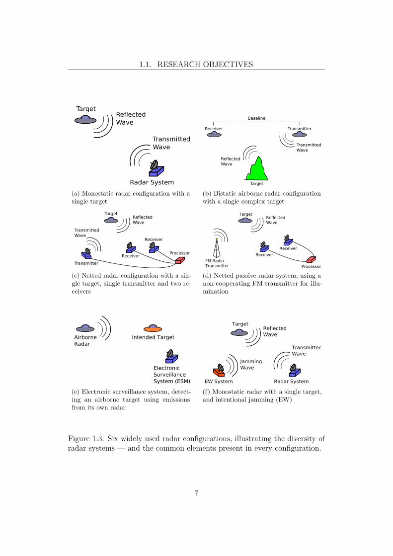
Figure 1.3 illustrates six possible radar configurations. In each of these
configurations there are one or more transmitters of electromagnetic signals,
one or more scatterers of those signals (targets), and one or more receivers
which capture and record the signals. This selection represents only a tiny
part of the diversity of radar systems, and clearly illustrates the need for a
flexible simulator.
Flexibility refers to the simulators applicability to a wide variety of radar
systems. Examples of supported systems include pulsed search radars (fig.
1.3(a)), netted radars (figs. 1.3(c) and 1.3(d)), airborne radars (figs. 1.3(b)
and 1.3(e)), electronic warfare systems (figs. 1.3(e) and 1.3(f)) and continuous
wave radar systems (fig. 1.3(d)).
The simulator was required to make no assumptions about waveforms;
system geometry and arrangement; system bandwidth; and numbers of tar-
gets, transmitters and receivers. The simulator will not perform any signal
processing on the output data, and makes no assumptions about the type of
signal processing that will be performed on the data.
Flexibility is a large part of the contribution of this work to the field of
signal-level radar simulation. Previous simulators have been typically focused
on a single application domain (monostatic pulsed systems in [15] and [2], or
SAR in [16] and [21], for example) or particular systems (the MARSIS radar
in [20], for example). The simulator presented in this work is intended to
be applicable to most radar application domains, and the majority of radar
systems.
Accuracy
The simulator is required to produce results which are accurate and precise
within a well described set of assumptions and bounding criteria. Limiting
assumptions and limitations on simulation accuracy must be clearly docu-
mented and discussed to ensure that the user is aware of these before applying
simulation results. Where tradeoffs require limitations on accuracy, the sim-
5

1.1. RESEARCH OBJECTIVES
ulator must ensure that the maximum possible accuracy and precision in
the parameters commonly used by radar signal processing algorithms are
retained.
Extensibility
The simulator is required to easily accept extensions and modifications to
allow for simulation of systems not included in the scope of the original
simulator. The extensibility requirement is two-fold. The simulator must
be able to accept extensions without modifying the base code, and the base
code must be easily modifiable to aid inclusion of extensions if the external
interfaces are inadequate.
Usability
ISO 9241-11 [22] defines usability in the context of software for office and
technical work as:
The extent to which a product can be used by specified users to
achieve specified goals with effectiveness, efficiency and satisfaction
in a specified context of use.
The simulator is required to maximize this property, ensuring that it is
effective and efficient to use. In the context of this work, usability is focused
on efficiency and effectiveness of use by an experienced user, not the ease of
learning to use the software for the first time.
Maximizing usability requires clear, well defined and consistent interfaces;
comprehensive documentation and predictable behaviour.
Portability
The simulator must not be restricted to any operating system or computer
architecture. The software will be written in standard C++ [23], a programming
language which is well supported on a variety of operating systems and
architectures. The extension mechanism is implemented in Python, with
interpreters available for all modern platforms and operating systems.
6
1.1. RESEARCH OBJECTIVES
(a) Monostatic radar configuration with asingle target
(b) Bistatic airborne radar configurationwith a single complex target
(c) Netted radar configuration with a sin-gle target, single transmitter and two re-ceivers
Reflected
Wave
FM Radio
Transmitter
Receiver
Receiver
Target
Processor
(d) Netted passive radar system, using anon-cooperating FM transmitter for illu-mination
Airborne
Radar
Intended Target
Electronic
Surveillance
System (ESM)
(e) Electronic surveillance system, detect-ing an airborne target using emissionsfrom its own radar
Radar System
Target
Transmitted
Wave
Reflected
Wave
EW System
Jamming
Wave
(f) Monostatic radar with a single target,and intentional jamming (EW)
Figure 1.3: Six widely used radar configurations, illustrating the diversity ofradar systems — and the common elements present in every configuration.
7
1.2. SIGNIFICANCE OF RESEARCH
1.2 Significance of Research
The exponential [24] rise of computing power available to engineers has lead to
a similar rise in interest in the simulation of complex systems. Simultaneously,
the rise of computing power and communications technology has lead to
increasing interest in the application of the ideas of sensor networks to radar
systems, greatly increasing the system level complexity, and hence difficulty
of analysis, of radars. Simulation can provide an invaluable tool tool to radar
researchers, engineers and operators.
The application of radar simulation in the research environment is to
reduce the difficulty and costs associated with testing new radar technologies
and approaches. Two traditional approaches are available to the researcher
wishing to analyse the performance of a new technology — prototyping and
closed form analysis. Simulation complements these two approaches by offering
a third tool — one which is much cheaper and quicker than prototyping, but
also easier and potentially more accurate than simplified analysis procedures.
The simulation model presented in this work is sufficiently flexible to allow
new technologies and hypotheses to be tested on a computer, reducing the
need for the development and testing of prototypes.
Accurate simulation adds a useful tool to the design process followed by
engineers working on the development of radar systems. The simulator reduces
the amount of time required for the development of systems by allowing
easy analysis of performance parameters of candidate designs. Similarly,
the application of simulation can reduce the amount of money required for
development by moving prototyping to a later stage in the design cycle —
when fewer design changes are likely to be required.
Education and training of radar engineers and operators is another area
where simulation can be used. The simulation can be used in the classroom to
demonstrate to students the effects of system parameters on radar performance,
and to allow students to freely experiment with these parameters. Combined
with a suitable interface, the simulator can also be used to develop scenarios
for the training of radar operators.
The application of radar simulation to research, development and education
8
1.3. STRUCTURE OF THESIS
provides a strong motivation for the development of a simulator which is
useful in all three of these roles.
1.3 Structure of Thesis
This chapter, Chapter 1, discusses the objectives of the research which has
been performed, the central hypothesis behind the research, and the approach
used to meet the required objectives. The final part of the chapter examines
the parts of the work which are believed to be novel contributions to the
field of radar. A brief discussion of past approaches to radar simulation is
included to support the objectives and approach. The key non-functional
requirements for the completed simulator are explained, and the importance
of each parameter examined.
Chapter 2 describes a flexible signal-level model for the simulation of
multistatic radar systems. The description includes discussions of the mod-
elling of the effects on radar signals of transmission, scattering, propagation
and reception. The model is applicable to radar systems with arbitrary
numbers of receivers and transmitters, and arbitrary numbers of scatterers in
the simulated environment.
Chapter 3 examines the generation of pseudonoise with statistical prop-
erties matching those obtained from the characterisation of oscillators in radar
hardware, and other sources of coloured noise in radar systems. An algorithm
for the efficient generation of coloured pseudonoise samples for the purposes
of radar simulation is described.
A model for clock generation in radar systems is presented, based on
existing models of timing sources and oscillators. Key performance parameters
for radar timing sources are discussed in the context of simulation of the
effects of degradation of these parameters.
Chapter 4 examines the development of a radar simulator using the
models and algorithms presented in Chapters 2 and 3. The design of the
software is presented and discussed, and justification for the choices made
during implementation is presented.
An overview of the software engineering design process is presented, with
9

1.4. STATEMENT OF ORIGINALITY
an examination of the efficient implementation of the simulation model on
parallel computers. The implementation of the simulator in C++ and the
extension mechanism in Python is presented, with a discussion of the key
performance parameters identified during implementation.
Chapter 5 presents the experimental validation and verification process
which has been undertaken to ensure the accuracy of simulation results. The
design of the equipment and experiments used for this verification process
is presented, along with the design of simulation scenarios matching these
experiments. Validation results from the NetRad netted radar system and
from an experimental sonar system are presented. Comparisons of simulation
and measurement results with theoretically expected values are presented and
analysed.
Chapter 6 concludes the work, and presents a list of possible future
extensions to the work presented here.
1.4 Statement of Originality
The candidate believes that the following parts of this work constitute original
contributions to the field of radar:
• The flexible simulation model, presented in Chapter 2, which allows
signal level simulations of radar systems with arbitrary number of trans-
mitters and receivers and arbitrary waveforms. This model is applicable
to a wide variety of types of radar systems, including multistatic, contin-
uous wave, and carrier-free systems. The flexibility and completeness of
this model exceeds that of the simulation models presented in existing
literature.
• An algorithm for the efficient generation of coloured pseudonoise se-
quences matching the measured characteristics of oscillators, presented
in Chapter 3.
• An algorithm for the efficient generation of sparse sequences of coloured
pseudonoise, presented in Chapter 3. This algorithm efficiently generates
10

1.4. STATEMENT OF ORIGINALITY
the pulsed sequences of coloured pseudonoise required for simulation of
pulse radar systems, while preserving the long memory nature of the
underlying noise generation process.
• The application of finite impulse response (FIR) subsample delay filters,
generated at runtime, to the accurate simulation of delay effects, includ-
ing both propagation delay and apparent delays caused by timing jitter,
in a digital radar simulator. This development allows the simulator
to accurately simulate the effects of these delays on any type of radar
waveform.
• The application of FIR subsample delay filters, generated at runtime,
to the accurate simulation of Doppler and phase effects in carrier-free
and continuous wave (CW) radar systems.
• The development of a flexible, extensible and freely available simulator
for multistatic and netted radar systems. The flexibility of the simulator
described in this work exceeds that of other freely available and well
described simulators. The simulator can be used to simulate radar
systems with arbitrary waveforms and arbitrary numbers of receivers,
transmitters and scatterers.
• The Monte Carlo simulation of the effects of phase noise on synthetic
aperture radar (SAR) and pulse-Doppler systems, as presented in Ap-
pendix A, is novel in its use of a phase noise generator capable of
generating realistic phase noise spectra.
11
Chapter 2
Discrete-Time Radar
Simulation Model
2.1 Introduction
This chapter describes a model for the simulation of a diverse range of radar
systems. The goal was to produce a model which is sufficiently generic to
adequately describe a wide variety of radar systems, while being sufficiently
specialised to allow efficient simulation. The simulation model is the most
important component of simulator development — the limitations of the
model are the limitations of the simulation, and the assumptions made during
model development are reflected in the simulator output.
The simulation model utilizes the superposition property of multistatic
radar systems, allowing the task of multistatic radar simulation to be de-
composed into multiple bistatic radar simulations. Each of these bistatic
radar simulations is performed using a two part bistatic radar simulation
model. This chapter provides justification for the use of superposition, and
describes the two parts of the radar simulation model in detail. In addition,
the parameters used for adjusting the model to match a particular system
are discussed, with emphasis on the relation of these parameters to physical
radar systems.
The simulation model was developed with software implementation in
12

2.1. INTRODUCTION
mind. A discussion of the implementation of this model in software is presented
in Chapter 4.
2.1.1 Superposition of Radar Systems
The principle of superposition applies to many of the key effects on signals in
radar systems. Expressed as a function f(x), these effects meet the criteria
of linearity — homogeneity:
f(αx) = αf(x), (2.1)
and additivity:
f(x+ y) = f(x) + f(y). (2.2)
Justifications for this observation will be given for the relevant phenomena in
this chapter. Based on the principle of superposition, a simple model for the
signals captured by receivers in multistatic radar systems can be formed. The
discrete-time signal yi[k] (where yi[k] is the kth sample of the bandlimited
signal yi(t)) received by receiver i, can be expressed as a sum of the modified
transmitted signals:
yi[n] =NT∑j=0
fij(xj[n]), (2.3)
where NT is the number of transmitters, xj is the signal transmitted by
transmitter j, and fij(x) is some linear (but not necessarily time invariant)
function which modifies the signal xj[n].
Considering the effects of transmission, propagation and reception sepa-
rately, the received signal can be expressed as:
yi[n] = Ri
(NT∑j=0
Eij(Tj(xj[n]))), (2.4)
where Ri is the effect of reception by receiver i, Eij is the environmental
effect of propagation along the path from transmitter j to receiver i, and Tj
is the effect of transmission by transmitter j. As these effects are not time
invariant, it is more accurate to express them as Ri(x, t), Tj(x, t) and Eij(x, t)
13

2.1. INTRODUCTION
Figure 2.1: Bistatic passive receiver system
— functions of both the signal and time. The key challenge in simulation is to
find the functions Ri(x, t), Eij(x, t) and Tj(x, t) which accurately model the
behaviour of the system under simulation.
2.1.2 Validity of Superposition
Modelling radar systems using equation 2.3 requires several assumptions to
be made about the behaviour of those systems. Theses assumptions are:
• No interaction between receivers. Each receiver in the radar system has
no effect on the signal received by the other receivers in the system.
This requires receivers to be passive listeners which do not emit or
absorb energy from the environment.
In the system illustrated in figure 2.1, under this assumption receiver
one will receive exactly the same signal at its antenna irrespective of
whether receiver two is present. This assumption is valid for most
common types of radar systems.
• No interaction between targets. No multiscatter returns — reflections
of energy from one target off another — are considered. The case of
multipath propagation is considered separately. In the system illustrated
in figure 2.2, three propagation paths via the targets exist: from the
transmitter to the first target and to the receiver; from the transmitter
to the second target and to the receiver; and from the transmitter to
14

2.1. INTRODUCTION
Figure 2.2: Bistatic radar system showing possible propagation paths.
the first target, to the second target then to the receiver. The third
path (marked with a dashed line in figure 2.2) is not considered by the
superposition model.
• No interaction between transmitters. Transmitters of electromagnetic
waves into the environment are assumed not to interact with other
transmitters — that is they do not absorb or otherwise modify the
waves transmitted by other transmitters. Similarly, superposition is
assumed to be valid for all interactions of electrodynamic waves and
targets. This assumption holds exactly in a vacuum, due to the linearity
of Maxwell’s equations in that medium [25], and holds closely in air at
all radar frequencies. These assumptions are examined in more detail
in Appendix B.
2.1.3 The Discrete Signal Model
For computer simulation of an analogue system, a discrete representation of
the analogue model is required. This representation is required to be both
discrete-time, as the computer cannot handle infinite numbers of samples,
and discrete in precision, as the computer cannot handle infinite precision.
The signals transmitted by radar systems can be separated logically into
two categories: lowpass signals and bandpass signals. As illustrated by figure
2.3, the Fourier transform of lowpass signals is limited to the band [−Ω,Ω].
The Fourier transform of a bandpass signal is constrained to a band around
the centre frequencies Ωc and −Ωc with bandwidth B = Ωh−Ωl. The majority
of radar signals are bandpass signals — lowpass signals are only widely used
15

2.1. INTRODUCTION
(a) Lowpass signal (b) Bandpass signal
Figure 2.3: Comparison of real valued lowpass and bandpass radar signals.
in carrier-free radar systems [26]. While the simulator supports both types of
radar signals, a significant reduction in computational costs can be achieved
through the use of a suitable model for bandpass signals.
The bandpass signal x(t) can be expressed as:
x(t) = a(t) cos (Ωct+ θ(t)) , (2.5)
where a(t) is the envelope and θ(t) the phase of x(t). Equivalently, x(t) can
be expressed in terms of inphase and quadrature parts [27]:
x(t) = xi(t) cos(Ωct)− xq(t) sin(Ωct), (2.6)
where xi(t) and xq(t) are real valued baseband signals and are referred to
as the inphase and quadrature parts of x(t). The complex envelope xl(t) is
defined as:
xl(t) = xi(t) + jxq(t). (2.7)
xl(t) is complex, situated at baseband, and has bandwidth Ωh − Ωl. The
Fourier transform of xl(t), Xl(ω) (Figure 2.4) is:
Xl(ω) = Xi(ω) + jXq(ω). (2.8)
For simulation of radar systems transmitting bandpass signals, it is conve-
nient to simulate using the complex envelope xl(t), and include phase effects
relevant to the original carrier frequency 2πΩc.
16

2.1. INTRODUCTION
Figure 2.4: Magnitude of the Fourier transform of the complex envelope ofthe signal x(t)
Discrete-Time Representation of Analogue Signals
The discrete-time signal x[n], equivalent to the continuous time signal x(t) is
defined as:
x[n] ≡ x
(n
fs
), (2.9)
where fs is the system sampling frequency. Provided that the signal x(t) is
bandlimited to the range from 0Hz to fs
2Hz [28, 29] and satisfies the Dirichlet
conditions [30] then,
x(t) =∞∑
n=−∞x[n] sinc (tfs − n) , (2.10)
where sinc(x) = sin(πx)/(πx). Performing the simulation using x[n] is there-
fore equivalent to simulating using x(t), provided that none of the simulated
effects cause x(t) to violate the criteria required for reconstruction. The sam-
pling rate fs must be chosen to ensure that the simulated x(t) remains limited
to the band [0, fs
2] when phase and frequency shift effects are considered.
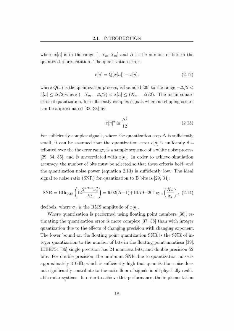
Quantization Effects on the Signal Model
Computer simulation requires mapping of the samples x[n] to a finite number
of bits of precision, known as quantization. For the fixed point (or integer)
case the quantization step, ∆, is defined [31] as:
∆ =Xm
2B, (2.11)
17
2.1. INTRODUCTION
where x[n] is in the range [−Xm, Xm] and B is the number of bits in the
quantized representation. The quantization error:
e[n] = Q(x[n])− x[n], (2.12)
where Q(x) is the quantization process, is bounded [29] to the range −∆/2 <
e[n] ≤ ∆/2 where (−Xm −∆/2) < x[n] ≤ (Xm −∆/2). The mean square
error of quantization, for sufficiently complex signals where no clipping occurs
can be approximated [32, 33] by:
e[n]2 u∆2
12(2.13)
For sufficiently complex signals, where the quantization step ∆ is sufficiently
small, it can be assumed that the quantization error e[n] is uniformly dis-
tributed over the the error range, is a sample sequence of a white noise process
[29, 34, 35], and is uncorrelated with x[n]. In order to achieve simulation
accuracy, the number of bits must be selected so that these criteria hold, and
the quantization noise power (equation 2.13) is sufficiently low. The ideal
signal to noise ratio (SNR) for quantization to B bits is [29, 34]:
SNR = 10 log10
(12
22B−2σ2x
X2m
)= 6.02(B−1)+10.79−20 log10
(Xm
σx
), (2.14)
decibels, where σx is the RMS amplitude of x[n].
Where quantization is performed using floating point numbers [36], es-
timating the quantization error is more complex [37, 38] than with integer
quantization due to the effects of changing precision with changing exponent.
The lower bound on the floating point quantization SNR is the SNR of in-
teger quantization to the number of bits in the floating point mantissa [39].
IEEE754 [36] single precision has 24 mantissa bits, and double precision 52
bits. For double precision, the minimum SNR due to quantization noise is
approximately 310dB, which is sufficiently high that quantization noise does
not significantly contribute to the noise floor of signals in all physically realiz-
able radar systems. In order to achieve this performance, the implementation
18
2.1. INTRODUCTION
must take care to ensure that floating point arithmetic operations are done
in the order which preserves maximum accuracy [39, 40].
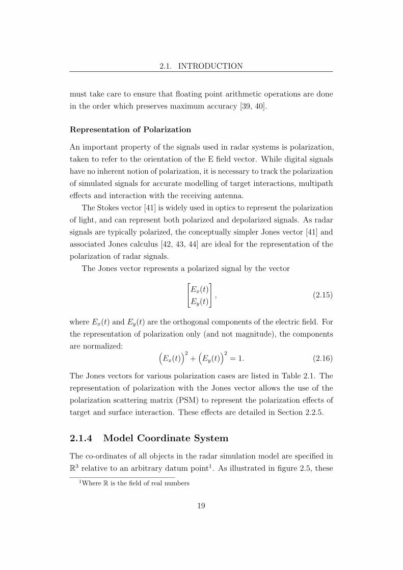
Representation of Polarization
An important property of the signals used in radar systems is polarization,
taken to refer to the orientation of the E field vector. While digital signals
have no inherent notion of polarization, it is necessary to track the polarization
of simulated signals for accurate modelling of target interactions, multipath
effects and interaction with the receiving antenna.
The Stokes vector [41] is widely used in optics to represent the polarization
of light, and can represent both polarized and depolarized signals. As radar
signals are typically polarized, the conceptually simpler Jones vector [41] and
associated Jones calculus [42, 43, 44] are ideal for the representation of the
polarization of radar signals.
The Jones vector represents a polarized signal by the vectorEx(t)Ey(t)
, (2.15)
where Ex(t) and Ey(t) are the orthogonal components of the electric field. For
the representation of polarization only (and not magnitude), the components
are normalized: (Ex(t)
)2+(Ey(t)
)2= 1. (2.16)
The Jones vectors for various polarization cases are listed in Table 2.1. The
representation of polarization with the Jones vector allows the use of the
polarization scattering matrix (PSM) to represent the polarization effects of
target and surface interaction. These effects are detailed in Section 2.2.5.
2.1.4 Model Coordinate System
The co-ordinates of all objects in the radar simulation model are specified in
R3 relative to an arbitrary datum point1. As illustrated in figure 2.5, these
1Where R is the field of real numbers
19

2.1. INTRODUCTION
Table 2.1: Jones vectors corresponding to various polarization cases
Polarization Jones Vector
x Linear[
10
]y Linear
[01
]Left circular 1√
2
[1j
]Right circular 1√
2
[1j
]
Figure 2.5: Axes of the model coordinate system
coordinates can be specified in terms of the Cartesian coordinates (x, y, z),
or the spherical coordinates (r, ϕ, θ). In this document, to match common
usage in radar literature, the zenith angle ϕ is referred to as elevation and is
measured from the xy plane. The azimuthal plane angle θ is referred to as
azimuth and is measured from the x axis.
The coordinate system is not referenced to any particular direction on the
Earth — applications of the simulator model are free to choose any direction
and datum point as a reference. The advantage of this system over the
north referenced coordinate system commonly used in the radar field [45] is
flexibility and applicability to a wide variety of radar configurations — not
all terrestrial.
The conversion of geodesic coordinates to Cartesian coordinates relative to
20

2.2. ENVIRONMENT MODEL
(a) Transmission path from transmitterto receiver via target
(b) Direct transmission from transmitterto receiver
Figure 2.6: Transmission paths for transmitted energy from transmitter toreceiver.
an arbitrary datum point is a complex problem, and depends on the geodetic
system (such as WGS84 [46]) used for the measurement of the coordinates.
For even modest ranges care must be taken in ensuring that the conversion
to Cartesian coordinates accounts for the assumptions of the geodetic system
in use.
2.2 Environment Model
The environment model, Eij(x), predicts the effects of propagation of the
signal x through the environment from transmitter j to receiver i. This model
depends on the positions and relative velocities of the transmitter j, receiver
i and all targets during the simulation period, as well as the properties of the
transmitters, receivers and targets.
Through the application of the superposition principle (Section 2.1.1), the
environment model is only concerned with a single transmitter-receiver pair —
while the entire simulator can handle arbitrary numbers of such pairs.
Considering both the direct (Figure 2.6(b)) transmitter to receiver trans-
mission path, and the paths via targets (Figure 2.6(a)), the environment
model can be expressed as:
Eij(x) = PijDij(x) +S∑k=1
PijkDijk(x), (2.17)
where Pijk and Pij are the attenuation due to propagation, Dijk and Dij are
21

2.2. ENVIRONMENT MODEL
the phase and frequency (Doppler) effects due to range and relative motion
of receiver i, transmitter j and target k, and S is the number of targets in
the environment.
2.2.1 The Object Model
In order to calculate the effects of propagation through the environment, the
model is required to keep track of the positions and properties of all the
objects in the environment. This is achieved through the application of an
hierarchical object model. The object model consists of six types of objects;
two parent object types and four physically realizable object types.
Figure 2.7 illustrates the object model, with the four physical object types
marked in grey. The six types of objects are:
Platform The platform parent object keeps track of the motion and rotation
of its child objects. A platform object has a defined three dimensional
path through the simulated world, and a defined rotation around an
arbitrary axis. All other types of objects depend on a platform object,
and can move without restriction through the simulated environment.
Radar The radar parent object embodies the common properties of radar
transmitters and receivers. The modelling of time and frequency control,
antenna behaviour and synchronisation behaviour is handled by the
radar object. A radar object can contain either a single transmitter,
single receiver, or both.
Target Targets represent any object in the environment which absorbs energy
from the environment, then re-emits that energy. The target object
models the RCS (including bistatic RCS and time dependent RCS) and
other aspects of target behaviour. Target motion is modelled by the
parent platform object.
Surface Surfaces represent planes in the environment with purely specular
(as defined in [41]) reflection of radar energy. Surfaces are used to
simulate the effects of multipath propagation.
22

2.2. ENVIRONMENT MODEL
Figure 2.7: Heirarchy of objects in the object model
Transmitter Transmitters represent any object which transmits electromag-
netic energy into the environment. The transmitter object models the
transmission schedule, transmitted waveform and the properties of the
transmitted signal. Antenna behaviour is modelled by the parent Radar
object.
Receiver Receivers represent objects which receive electromagnetic energy
from the environment, then capture a record of that energy. The receive
object models the receive schedule (receive window) and the properties
of the receiver hardware (such as gain, ADC precision, etc).
The object model keeps track of any number of each type of object. No
restrictions are placed on the arrangement, movement or rotation of objects
in the object model.
2.2.2 The Bistatic Radar Equation
The propagation attenuation for target paths is calculated using the bistatic
radar equation [26, 47, 48]. The power radiated in the direction of receiver i
by target k, illuminated by transmitter j is:
Pg = PtGtLtLptσb
4πR2kj
, (2.18)
where Pt is the transmitted power, Gt the transmitter antenna gain in the
direction of the target, Lt the loss in the transmitter, Lpt is the excess
propagation loss, σb the bistatic radar cross section (RCS) for the transmitter
and receiver angles, and Rkj the range between transmitter j and target k.
23

2.2. ENVIRONMENT MODEL
The power received by the antenna of receiver i from target k is:
Pr = PgGrLrLprλ
2
(4π)2R2ik
, (2.19)
where Gr is the receiver antenna gain in the direction of the target, Lr the
losses in the receiver system, Lpt is the excess propagation loss, λ is the
wavelength at the centre frequency of the radar system, and Rik the range
between target k and receiver i. The total received power is therefore:
Pr = PtGtGrLtLrLprLptσbλ
2
(4π)3R2kjR
2ik
. (2.20)
From a similar derivation, without including the target effects, the power
received by receiver i directly from transmitter j is:
Pr = PtGtGrLtLrλ
2
(4π)2R2ij
, (2.21)
where Rij is the range from i to j.
2.2.3 Phase and Frequency Effects
The finite speed of propagation of electromagnetic energy through the envi-
ronment introduces a delay on the arrival time of the transmitted signal at
the receiver.
For bandpass signals, we can consider the propagation delay to have two
separate effects on the signal — phase delay and group delay. From the
definition of the complex baseband signal (equation 2.7), a delay by the
propagation time τ can be expressed as:
xshift[n] = xi[n+ τfs] cos(2πf0(t+ τ))− xq[n+ τfs] sin(2πf0(t+ τ)), (2.22)
where fs is the system sample rate and f0 = Ωc
2π. The delay on the complex
baseband signal xl[n], τfs samples, is the group delay, and the delay on the
carrier signal, 2πf0τ radians, is the phase delay. For lowpass signals, where
24

2.2. ENVIRONMENT MODEL
Figure 2.8: Block diagram of the effect of phase shift on quadrature reception.Upmixers include suitable low pass filters.
simulation is performed at the full system sample rate, only the group delay
is considered.
Introducing a phase shift on the signal of a bandpass radar system, utilising
a quadrature upmixer and downmixer, introduces mixing of the inphase and
quadrature channels. For the system in figure 2.8, the signal after the carrier
phase shift θ, equivalent to time delay by τ = θ/ (2πf0) seconds, is:
xshift[n] = I[n+ τfs] cos(2πf0t+ θ)−Q[n+ τfs] sin(2πf0t+ θ). (2.23)
The output channel is therefore:
Iout[n] = xshift[n] cos(2πf0t), and (2.24)
Qout[n] = xshift[n] sin(2πf0t) (2.25)
which is equal to:
Iout[n] = I[n+ τfs] cos(θ)−Q[n+ τfs] sin(θ), and (2.26)
Qout[n] = Q[n+ τfs] cos(θ) + I[n+ τfs] sin(θ). (2.27)
Considering only the time shift τ (and hence carrier phase shift θ), and using
the definition of the complex baseband signal in equation 2.7, the output of
the system in figure 2.8 is:
y[n] = xl[n+ τfs]ejθ. (2.28)
25

2.2. ENVIRONMENT MODEL
Equivalently, for lowpass signals, the output of the system is:
y[n] = xl[n+ τfs], (2.29)
and lowpass signals can clearly be considered to be a special case of baseband
signals where f0 = 0 and xl[n] is purely real. Where τfs /∈ Z, some interpola-
tion2 is required to meaningfully define xl[n + τfs]. The ideal definition is
based on bandlimited interpolation (equation 2.10), and an implementation
of this interpolation is presented in Section 4.3 on page 97.
The time delay τ is:
τ =Rjk +Rik
c, (2.30)
where Rjk and Rik are the transmitter-target and target-receiver ranges, and
c is the propagation speed. For radar applications c ≈ c0, where c0 is the
speed of light in a vacuum (299792458ms−1) [49]. For radar in air, c = c0n
,
where n is the refractive index of air, approximately 1 + 2.92× 10⁻⁴ at STP
[41]. The propagation speed c in air is therefore ∼ 299704746ms−1. For sonar
simulations, c is the speed of sound in the relevant medium.
In both narrowband and wideband cases, the group delay is equal to τ
seconds. In the narrowband case, the phase delay experienced by the carrier
is:
θ = 2πf0Rjk +Rik
c= 2πf0τ. (2.31)
The Doppler Effect
The Doppler effect for velocities much less than the speed of light is widely
expressed in terms of frequency. For monostatic geometries, the Doppler shift
[26, 50] is:
fd =2vrλ, (2.32)
where fd is the Doppler shift, and v is the radial velocity of the target relative
to the radar system and vr c. For bistatic systems:
fd =vr + vtλ
, (2.33)
2Where Z is the ring of integers
26

2.2. ENVIRONMENT MODEL
where vt and vr are the radial velocities of the target relative to the transmitter
and receiver and |vt| + |vr| c. While these equations do not take the
relativistic Doppler effect into account, they match the relativistic Doppler
prediction within 0.1% for total velocities less than 6× 10⁵ms−1. Expressed
in terms of range, the instantaneous Doppler shift is:
fd =f0
c
(dRik
dt+dRjk
dt
), (2.34)
for propagation via a target. Substituting equation 2.30 into equation 2.34,
fd = f0dτ
dt. (2.35)
From equations 2.31 and 2.35 it is clear that the Doppler shift is equal to
a change in phase and group delay corresponding to the change in range.
In a discrete-time model, it it therefore not necessary to consider Doppler
separately from the propagation delay τ for each sample. If τ is calculated
per-sample, and fd(t) is properly sampled at fs, it is not necessary to consider
the Doppler effect at all for either the bandpass or lowpass cases.
It is necessary to ensure that xl[n] remains correctly sampled after the
application of time dependent phase shifts. Where B is the bandwidth of
xl[n], the sampling frequency fs must be chosen such that:
fs > 2 (B + fd) , (2.36)
in order to avoid aliasing.
2.2.4 Target Model
Targets in the simulator model are assumed to be point-like reflectors with a
specified bistatic RCS. The bistatic RCS is a function of both the measured
cross section of the target, and probabilistic variations in the apparent RCS
of the target.
27

2.2. ENVIRONMENT MODEL
0 1 2 3 4 5 60
0.2
0.4
0.6
0.8
1
σ
Pro
babi
lity
Swerling 1 CDFSwerling 3 CDFSwerling 1 PDFSwerling 3 PDF
Figure 2.9: Cumulative density functions and probability density functionsfor Swerling cases 1 and 3 (σ = 1)
The Swerling Cases
Statistical models of time dependent radar cross section fluctuations are
widely applied in the simulation and analysis of radar systems [26, 50, 51].
While the most commonly applied statistical models are the Swerling cases
[52, 53, 54], these have been found to be inadequate for many common radar
applications [55, 56, 57]. While many alternatives [58, 21, 59] are available,
the chi-square target model proposed by Swerling [57] is attractive as it is
easily implemented and widely applicable.
The traditional Swerling RCS fluctuation model [54, 53, 51] breaks RCS
fluctuations down into five cases. For cases one and two, the RCS probability
density function is:
p(σ) =1
σexp
(−σσ
)σ ≥ 0, (2.37)
where σ is the RCS and σ is the mean value of the RCS. In case one, the RCS
is constant throughout a scan, and is uncorrelated between scans. In case
two, the RCS is constant throughout a pulse, and is uncorrelated between
adjacent pulses.
28
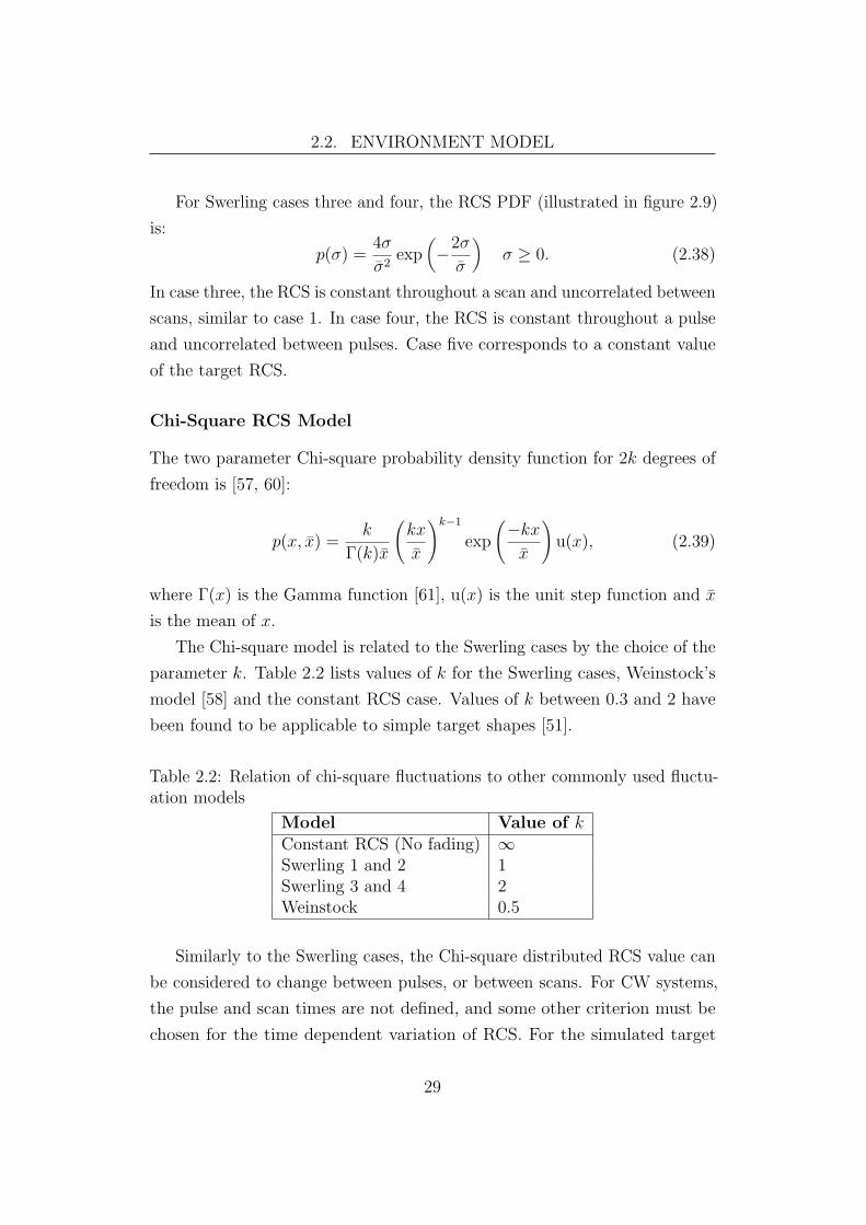
2.2. ENVIRONMENT MODEL
For Swerling cases three and four, the RCS PDF (illustrated in figure 2.9)
is:
p(σ) =4σ
σ2exp
(−2σ
σ
)σ ≥ 0. (2.38)
In case three, the RCS is constant throughout a scan and uncorrelated between
scans, similar to case 1. In case four, the RCS is constant throughout a pulse
and uncorrelated between pulses. Case five corresponds to a constant value
of the target RCS.
Chi-Square RCS Model
The two parameter Chi-square probability density function for 2k degrees of
freedom is [57, 60]:
p(x, x) =k
Γ(k)x
(kx
x
)k−1
exp
(−kxx
)u(x), (2.39)
where Γ(x) is the Gamma function [61], u(x) is the unit step function and x
is the mean of x.
The Chi-square model is related to the Swerling cases by the choice of the
parameter k. Table 2.2 lists values of k for the Swerling cases, Weinstock’s
model [58] and the constant RCS case. Values of k between 0.3 and 2 have
been found to be applicable to simple target shapes [51].
Table 2.2: Relation of chi-square fluctuations to other commonly used fluctu-ation models
Model Value of kConstant RCS (No fading) ∞Swerling 1 and 2 1Swerling 3 and 4 2Weinstock 0.5
Similarly to the Swerling cases, the Chi-square distributed RCS value can
be considered to change between pulses, or between scans. For CW systems,
the pulse and scan times are not defined, and some other criterion must be
chosen for the time dependent variation of RCS. For the simulated target
29

2.2. ENVIRONMENT MODEL
model in CW systems, the RCS changes every T seconds, with the values
between changes interpolated with cubic spline interpolation [62].
While the Chi-square distributed RCS model is widely used, and applicable
in many situations, other models for RCS fluctuations have been developed,
which can offer better fits to experimental data in some cases. Alternatives to
the chi-square model include models based on the Rician distribution [63], log-
normal distribution [64, 65], Legendre polynomials [21] and the non-central
Gamma distribution [59].
Target RCS Variation with Angle
The variation in radar cross section with the arrival and departure angles is
as important to system performance as statistical fluctuations in the target
RCS [66, 67]. The target model considers both the monostatic and bistatic
radar cross sections of the target, by defining RCS as a function of the angle
of arrival, angle of departure and the signal polarisation angle. The bistatic
RCS σb in the radar equation (equation 2.20) is therefore [68]:
σb = σ (θa, φa, θd, φd, φs) , (2.40)
where θa and θd are the azimuth angles of arrival and departure, φa and φd are
the elevation angles of arrival and departure and φs is the signal polarization.
Where accurate measurements of bistatic RCS are available, σb can be
interpolated from the measured data. Similarly, a variety of numerical methods
are available for the calculation of bistatic RCS from target models [68, 69].
The availability of such data is useful for ensuring the accuracy of simulations.
Bistatic RCS measurements and simulations are not always available for
simulations. Where monostatic measurements at f0 cos(β/2) are available,
for bistatic angle β, the monostatic RCS along the bisector of the bistatic
angle accurately estimates the bistatic RCS for small β [70, 69], typically
β < 5 [48].
To obtain the PDF of the bistatic RCS for a single target in the bistatic
configuration, the bistatic RCS function σ (θa, φa, θd, φd, φs) is substituted for
the mean RCS in equation 2.39. Discrete samples matching this RCS are
30
2.2. ENVIRONMENT MODEL
generated, per look or per pulse, and are used in equation 2.20.
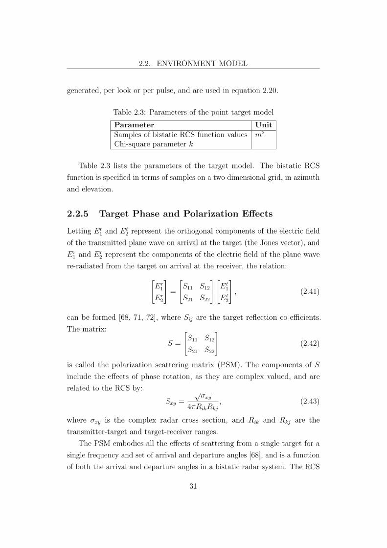
Table 2.3: Parameters of the point target model
Parameter UnitSamples of bistatic RCS function values m2
Chi-square parameter k
Table 2.3 lists the parameters of the target model. The bistatic RCS
function is specified in terms of samples on a two dimensional grid, in azimuth
and elevation.
2.2.5 Target Phase and Polarization Effects
Letting Et1 and Et
2 represent the orthogonal components of the electric field
of the transmitted plane wave on arrival at the target (the Jones vector), and
Er1 and Er
2 represent the components of the electric field of the plane wave
re-radiated from the target on arrival at the receiver, the relation:Er1
Er2
=
S11 S12
S21 S22
Et1
Et2
, (2.41)
can be formed [68, 71, 72], where Sij are the target reflection co-efficients.
The matrix:
S =
S11 S12
S21 S22
(2.42)
is called the polarization scattering matrix (PSM). The components of S
include the effects of phase rotation, as they are complex valued, and are
related to the RCS by:
Sxy =
√σxy
4πRikRkj
, (2.43)
where σxy is the complex radar cross section, and Rik and Rkj are the
transmitter-target and target-receiver ranges.
The PSM embodies all the effects of scattering from a single target for a
single frequency and set of arrival and departure angles [68], and is a function
of both the arrival and departure angles in a bistatic radar system. The RCS
31

2.2. ENVIRONMENT MODEL
model without considering phase and polarization effects corresponds to the
PSM:
S =1
4πRikRkj
√σ 0
0√σ
, (2.44)
for σ ∈ R. Where phase effects are considered, S remains diagonal, but
complex values of σ are included.
The voltage received by the receiver j is [68]:
√Pr ∝
∣∣∣∣∣~rj ·Er
1
Er2
∣∣∣∣∣, (2.45)
where ~rj is the polarization vector of the receiver j. Combining with the
bistatic radar equation (equation 2.20) the return power becomes:
√Pr =
∣∣∣∣∣~rj ·Er
1
Er2
∣∣∣∣∣√PtGtGrLtLrλ2
4π, (2.46)
and the propagation phase shift (equation 2.31) becomes:
λ = arg
~rj ·Er
1
Er2
+ 2πf0Rjk +Rik
c(2.47)
The RCS function can be specified to produce either real scalar RCS
values or the components of the PSM. The specified RCS samples (Table 2.3)
can therefore be either scalar or matrix values.
2.2.6 Bistatic Multipath Propagation
In an ideal bistatic radar system with a single target, two paths exist for
energy to pass from the transmitter to the receiver: directly, or via a target.
The addition of a plane with purely specular reflection to the configuration
increases the total number of available paths to six, assuming that all objects
are on the same side of the plane. The six paths are illustrated in figure
2.11(b). Propagation along any of the reflected paths alters the signal by
attenuation, phase shift, and a change in polarization.
32
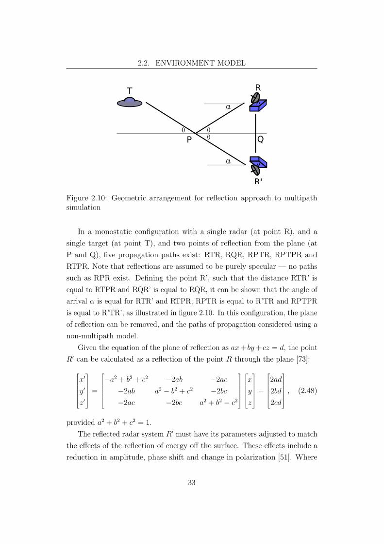
2.2. ENVIRONMENT MODEL
Figure 2.10: Geometric arrangement for reflection approach to multipathsimulation
In a monostatic configuration with a single radar (at point R), and a
single target (at point T), and two points of reflection from the plane (at
P and Q), five propagation paths exist: RTR, RQR, RPTR, RPTPR and
RTPR. Note that reflections are assumed to be purely specular — no paths
such as RPR exist. Defining the point R’, such that the distance RTR’ is
equal to RTPR and RQR’ is equal to RQR, it can be shown that the angle of
arrival α is equal for RTR’ and RTPR, RPTR is equal to R’TR and RPTPR
is equal to R’TR’, as illustrated in figure 2.10. In this configuration, the plane
of reflection can be removed, and the paths of propagation considered using a
non-multipath model.
Given the equation of the plane of reflection as ax+ by+ cz = d, the point
R′ can be calculated as a reflection of the point R through the plane [73]:
x′
y′
z′
=
−a2 + b2 + c2 −2ab −2ac
−2ab a2 − b2 + c2 −2bc
−2ac −2bc a2 + b2 − c2
x
y
z
−
2ad
2bd
2cd
, (2.48)
provided a2 + b2 + c2 = 1.
The reflected radar system R′ must have its parameters adjusted to match
the effects of the reflection of energy off the surface. These effects include a
reduction in amplitude, phase shift and change in polarization [51]. Where
33

2.2. ENVIRONMENT MODEL
these effects have been included, the sum of the signals at R and R′ without
the surface is equal to the signal at R with the reflecting surface.
The complex envelope of the simulated reflected signal xr[n] can be
expressed in terms of the complex envelope of the direct signal received from
the transformed receiver xe[n] by:
xr[n] = ρxe[n]ejφ, (2.49)
where ρ and φ are dependent on the properties of the surface of reflection.
This model considers only reflection from smooth surfaces, with a roughness
correction factor.
Reflection Properties of Smooth Surfaces
Long [71] defines the reflection coefficient, or proportion of the total energy
in the beam illuminating a surface reflected, as:
Reflection coefficient = ρsDR, (2.50)
where ρs is the reflection coefficient for a smooth earth, D is the reduction in
reflection energy caused by curvature of the surface, and R is the reduction
due to surface roughness. As the geometry in figure 2.10 is not valid for
curved surfaces, the factor D is assumed to be unity. The roughness factor
R, where 0 ≤ R ≤ 1 depends on the roughness of the surface, where 0 and 1
correspond to extremely rough and completely smooth.
The factor ρ is dependent on the frequency and polarization of the signal
and the angle of incidence (θ in figure 2.10), as well as on the electromagnetic
properties of the surface. Where this discussion refers to vertical and horizontal
polarization, it will mean perpendicular to and parallel to the surface of
reflection. For a surface with permittivity K and conductivity σ, the complex
dielectric constant ε is given by [71]:
ε =1
ε0
(K − jσ
2πf0
), (2.51)
34

2.2. ENVIRONMENT MODEL
(a) Transmission paths
(b) Receive paths
(c) Multiple paths replaced with multiple receivers andtransmitters
Figure 2.11: Equivalence of rearrangement of system geometry and multipathpropagation
35
2.2. ENVIRONMENT MODEL
where f0 is the radar centre frequency and ε0 is the electric constant [74].
For horizontal and vertical polarization respectively, the complex reflection
coefficients are:
Γh = ρhe−jφh =
sin β −√ε− cos2 β
sin β +√ε− cos2 β
(2.52)
Γv = ρve−jφv =
ε sin β −√ε− cos2 β
ε sin β +√ε− cos2 β
, (2.53)
where β = π − θ. As Γ is a complex quantity, both a magnitude change
(ρ) and phase shift (φ) occur during reflection. Equations 2.53 and 2.52 are
equivalent to the Fresnel equations [41] for linearly polarized waves.
The multipath model presented here is limited — especially by the smooth
surface and flat earth assumptions — but will provide useful results in cases
where the underlying assumptions are valid. The extensibility of the simulator
software (see Chapter 4) allows more complex models to be included, where
necessary.
Polarization and Phase in Multipath Propagation
For the case of linear polarization, the phase, amplitude and polarization
effects of reflection off a surface can be expressed in terms of a polarization
scattering matrix (see Section 2.2.5 on page 31).
For linear polarization in cases where no depolarization occurs (such as
for a smooth sea surface),
S =
Γh 0
0 Γv
. (2.54)
For circular polarization the PSM must be transformed using the Jones
calculus [42], and S becomes
S =1
2
1 −j1 j
Γh 0
0 Γv
1 1
−j j
. (2.55)
Where depolarization occurs, the matrix S is not diagonal, and the change
in polarization is expressed in the components S12 and S21. The simulation
36

2.3. HARDWARE MODEL
model accepts surface scattering parameters as either a single complex scalar
Γ, or the complete PSM for the surface interaction.
Table 2.4: Parameters of multipath simulation surface
Parameter UnitsCoefficients of plane equation mRoughness factor (R)Relative dielectric constant (ε), orReflection coefficient (Γ), orPSM coefficients
The parameters for the multipath surface model are listed in Table 2.4.
If the dielectric constant is specified, equations 2.52 and 2.53 are used with
equation 2.54 to derive the PSM. If a single value of Γ is specified, the PSM
S =
Γ 0
0 Γ
(2.56)
is used. Coefficients of the plane equation ax+ by + cz = d are specified in
meters, relative to the centre of the global coordinate system.
2.3 Hardware Model
Modelling the receiver (Ri(x, t)) and transmitter (Tj(x, t)) effects requires
modelling the behaviour of the radar system hardware and the effects of
that hardware on the radar signal. The diversity of radar hardware requires
that the model be sufficiently flexible to include all relevant effects. For
accurate simulation, the performance parameters of the radar hardware under
simulation must be mapped onto the model parameters.
2.3.1 The Transmitter Model
The transmitter model, illustrated in figure 2.12, consists of six parts: the
signal source, the time and frequency source, the quadrature upmixer, the
power amplifier, a bandpass filter, and the transmit antenna.
37

2.3. HARDWARE MODEL
Figure 2.12: Block diagram of the transmitter hardware model
The Signal Source and Quadrature Upmixer
The signal source and quadrature upmixer model the devices in a radar system
which generate the signal to be transmitted. The signal source generates
the inphase (real) and quadrature (imaginary) parts of the complex envelope
xl[n], samples of the continuous complex envelope xl(t). The quadrature
upmixer mixes this signal up to the transmit frequency.
In many types of radar systems, the output signal x(t) is not generated
with a structure similar to that illustrated in figure 2.12. Where these signals
can be mathematically represented as bandpass signals, their generation is
still adequately represented by figure 2.12 as the signal source and quadrature
upmixer together are mathematically equivalent to equation 2.6.
In modern digital radar systems (such as NetRad [75, 76, 77, 78], or
HYCAM [79]) the signal source is likely to model a direct digital synthesizer
(DDS), or a digital to analogue converter (DAC). For other types of radar
systems, the signal source and quadrature upmixer can model a frontend
based on magnetrons [80], Klystrons [51], IMPATT oscillators [81, 82], or
many other technologies [51].
The effects of local oscillator phase noise on the upmixing process, and of
timing source jitter on the signal source are considered in Chapter 3.
The parameters of the signal source are the system sampling frequency
(fs), and the digital samples of the complex envelope of the waveform to be
simulated. The parameter of the quadrature upmixer is the local oscillator
frequency (f0). The transmit schedule defines when the transmitter will
38

2.3. HARDWARE MODEL
transmit.
Time and Frequency Source
The time and frequency source is the source of the transmitter’s concept of
absolute time, relative time and frequency. The effects of imperfections in
the transmitter’s concept of time are complex, and are examined in detail
in Chapter 3. In addition to modelling the time and frequency references of
the transmitter, the timing source controls the transmit schedule, possibly
synchronising with receivers or other transmitters in the modelled system.
The parameters of the time and frequency source are the oscillator centre
frequency, oscillator phase noise curve, phase offset and frequency offset.
Power Amplifier
The power amplifier models the gain stages in the transmitter. The output
of the signal source and upmixer is normalized to the range [−1, 1], and the
power amplifier provides the gain necessary to achieve the required transmit
power.
The parameters of the power amplifier are the output power, noise tem-
perature [83] and noise bandwidth.
Bandpass Filter
The bandpass filter included before the antenna is not explicitly simulated —
it is included in the model to indicate the bandpass nature of the discrete-time
simulation model. Physical radar systems are also bandpass in nature, and
the simulation sample rate should be chosen to reflect the limited bandwidth
of the physical system being simulated.
Antenna
The antenna is modelled as a two dimensional (azimuth and elevation) far
field gain pattern. As the simulation does not consider nearfield effects, no
details of antenna construction or geometry are required. The phase centre
39
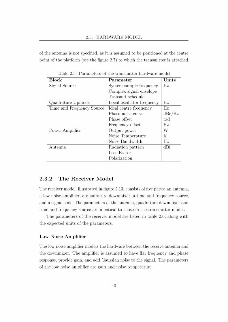
2.3. HARDWARE MODEL
of the antenna is not specified, as it is assumed to be positioned at the centre
point of the platform (see the figure 2.7) to which the transmitter is attached.
Table 2.5: Parameters of the transmitter hardware model
Block Parameter UnitsSignal Source System sample frequency Hz
Complex signal envelopeTransmit schedule
Quadrature Upmixer Local oscillator frequency HzTime and Frequency Source Ideal centre frequency Hz
Phase noise curve dBc/HzPhase offset radFrequency offset Hz
Power Amplifier Output power WNoise Temperature KNoise Bandwidth Hz
Antenna Radiation pattern dBiLoss FactorPolarization
2.3.2 The Receiver Model
The receiver model, illustrated in figure 2.13, consists of five parts: an antenna,
a low noise amplifier, a quadrature downmixer, a time and frequency source,
and a signal sink. The parameters of the antenna, quadrature downmixer and
time and frequency source are identical to those in the transmitter model.
The parameters of the receiver model are listed in table 2.6, along with
the expected units of the parameters.
Low Noise Amplifier
The low noise amplifier models the hardware between the receive antenna and
the downmixer. The amplifier is assumed to have flat frequency and phase
response, provide gain, and add Gaussian noise to the signal. The parameters
of the low noise amplifier are gain and noise temperature.
40

2.3. HARDWARE MODEL
Figure 2.13: Block diagram of the receiver hardware model
Signal Sink
The signal sink models the method used for capturing the signal seen at the
receiver. The signal sink does not perform any processing of the captured
data except for simulation of signal quantization. The parameters of the
signal sink are the system sample frequency, receive schedule, and number of
bits in the ADC.
Table 2.6: Parameters of the receiver hardware model
Block Parameter UnitsSignal Sink System sample frequency Hz
ADC bitsReceive schedule
Quadrature Downmixer Local oscillator frequency HzTime and Frequency Source Ideal centre frequency Hz
Phase noise curve dBc/HzPhase offset radFrequency offset Hz
Low Noise Amplifier GainNoise Temperature KNoise Bandwidth Hz
Antenna Radiation pattern dBiLoss FactorPolarization
41

2.4. CONCLUSION
2.4 Conclusion
A model for the simulation of radar systems has been developed. The goal of
the model was to retain as much flexibility as possible, while having sufficient
descriptive power to clearly define radar simulation problems. In the interests
of simulation flexibility, where particular models (such as the Chi-square RCS
variation model in Section 2.2.4) for physical behaviours have been used, the
simulation system allows these models to be bypassed or replaced.
The radar simulation model presented here is an hierarchical model (see
figure 2.7 on page 23) recognising four physically realizable object types. Each
of these object types has a number of parameters which set their properties
and behaviour. Of these four object types three (receivers, transmitters
and targets) can exist in any number in the simulated environment and one
(surfaces) can only have a single embodiment. The simulation model breaks
a complex simulation problem down into simpler simulations of monostatic
and bistatic radar configurations, through application of the superposition
principle.
Implementation of the radar simulation model as a computer program is
discussed in Chapter 4.
42
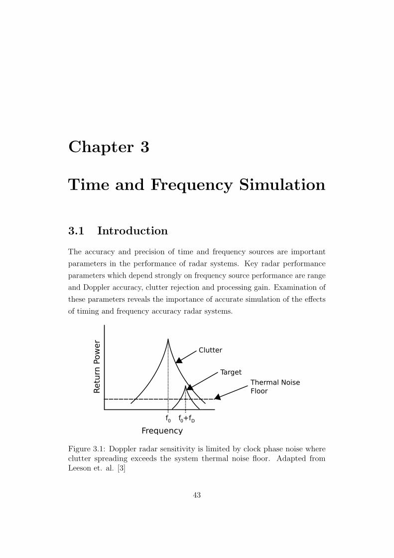
Chapter 3
Time and Frequency Simulation
3.1 Introduction
The accuracy and precision of time and frequency sources are important
parameters in the performance of radar systems. Key radar performance
parameters which depend strongly on frequency source performance are range
and Doppler accuracy, clutter rejection and processing gain. Examination of
these parameters reveals the importance of accurate simulation of the effects
of timing and frequency accuracy radar systems.
Figure 3.1: Doppler radar sensitivity is limited by clock phase noise whereclutter spreading exceeds the system thermal noise floor. Adapted fromLeeson et. al. [3]
43
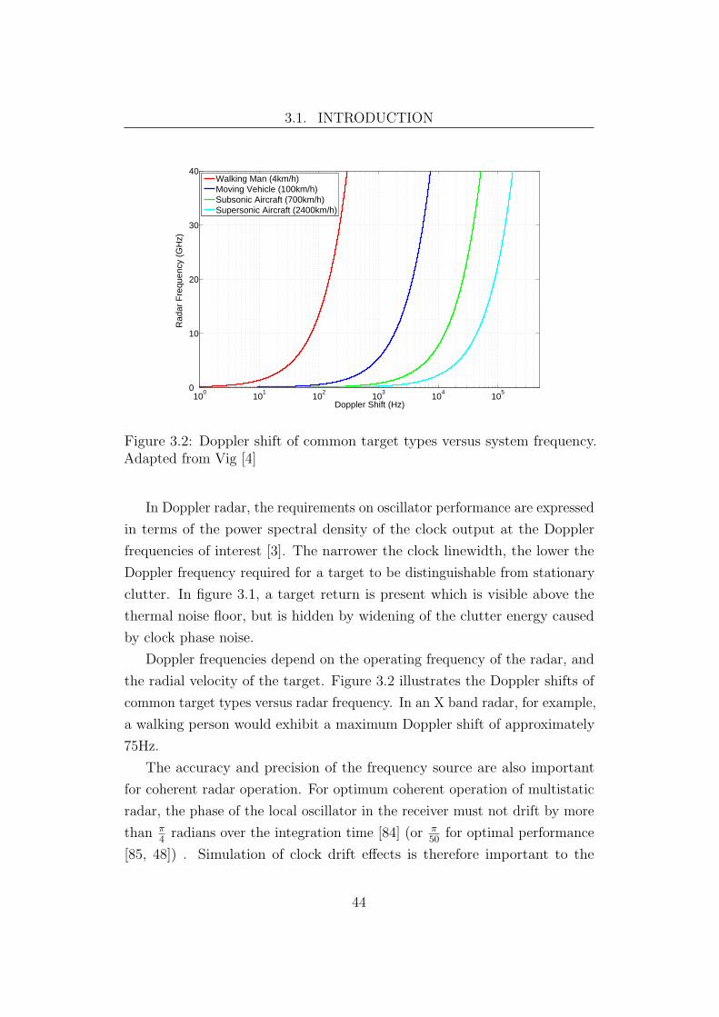
3.1. INTRODUCTION
100
101
102
103
104
1050
10
20
30
40
Doppler Shift (Hz)
Rad
ar F
requ
ency
(G
Hz)
Walking Man (4km/h)Moving Vehicle (100km/h)Subsonic Aircraft (700km/h)Supersonic Aircraft (2400km/h)
Figure 3.2: Doppler shift of common target types versus system frequency.Adapted from Vig [4]
In Doppler radar, the requirements on oscillator performance are expressed
in terms of the power spectral density of the clock output at the Doppler
frequencies of interest [3]. The narrower the clock linewidth, the lower the
Doppler frequency required for a target to be distinguishable from stationary
clutter. In figure 3.1, a target return is present which is visible above the
thermal noise floor, but is hidden by widening of the clutter energy caused
by clock phase noise.
Doppler frequencies depend on the operating frequency of the radar, and
the radial velocity of the target. Figure 3.2 illustrates the Doppler shifts of
common target types versus radar frequency. In an X band radar, for example,
a walking person would exhibit a maximum Doppler shift of approximately
75Hz.
The accuracy and precision of the frequency source are also important
for coherent radar operation. For optimum coherent operation of multistatic
radar, the phase of the local oscillator in the receiver must not drift by more
than π4
radians over the integration time [84] (or π50
for optimal performance
[85, 48]) . Simulation of clock drift effects is therefore important to the
44
3.2. STOCHASTIC MODEL OF FREQUENCY SOURCES
accurate simulation of the performance of coherent radar systems.
Time and frequency stability, and hence simulation of the effects of
instability, is critical in multistatic and netted radar systems. Relative drifts
and offsets in the phase and frequency of the timing sources in separate
nodes can seriously degrade system performance, and must be included in a
simulation of multistatic radar performance.
Timing instabilities can have a significant effect on the performance of
netted radar systems. For example, if timing accuracy is sufficient to operate
a netted radar system in coherent mode, the system signal to noise ratio
increases with the square of the number of nodes [86, 87]. In non-coherent
mode, the signal to noise ratio increases linearly with the number of nodes.
3.2 Stochastic Model of Frequency Sources
3.2.1 Definition of the Instantaneous Phase Deviation
An ideal oscillator produces the instantaneous output voltage Videal(t):
Videal(t) = V0 sin(2πv0t), (3.1)
where v0 is the nominal frequency of the oscillator, and V0 is the nominal
output voltage. In physically realizable systems, several errors reduce the
accuracy of the oscillator output — amplitude modulation (ε(t)), phase
fluctuations (ϕ(t)) and additive noise (V1(t)). Adding these error sources
creates a black box [88] model of the expected output of physically realizable
timing sources [89, 90, 91, 4]:
V (t) = (V0 + ε(t)) sin(2πv0t+ ϕ(t)) + V1(t). (3.2)
In this section, we assume that the additive noise V1(t), and amplitude
modulation ε(t), are much smaller than the oscillator output voltage V0, and
hence we do not consider these effects.
Using these assumptions, Barnes et. al. [89, 90] define the instantaneous
45
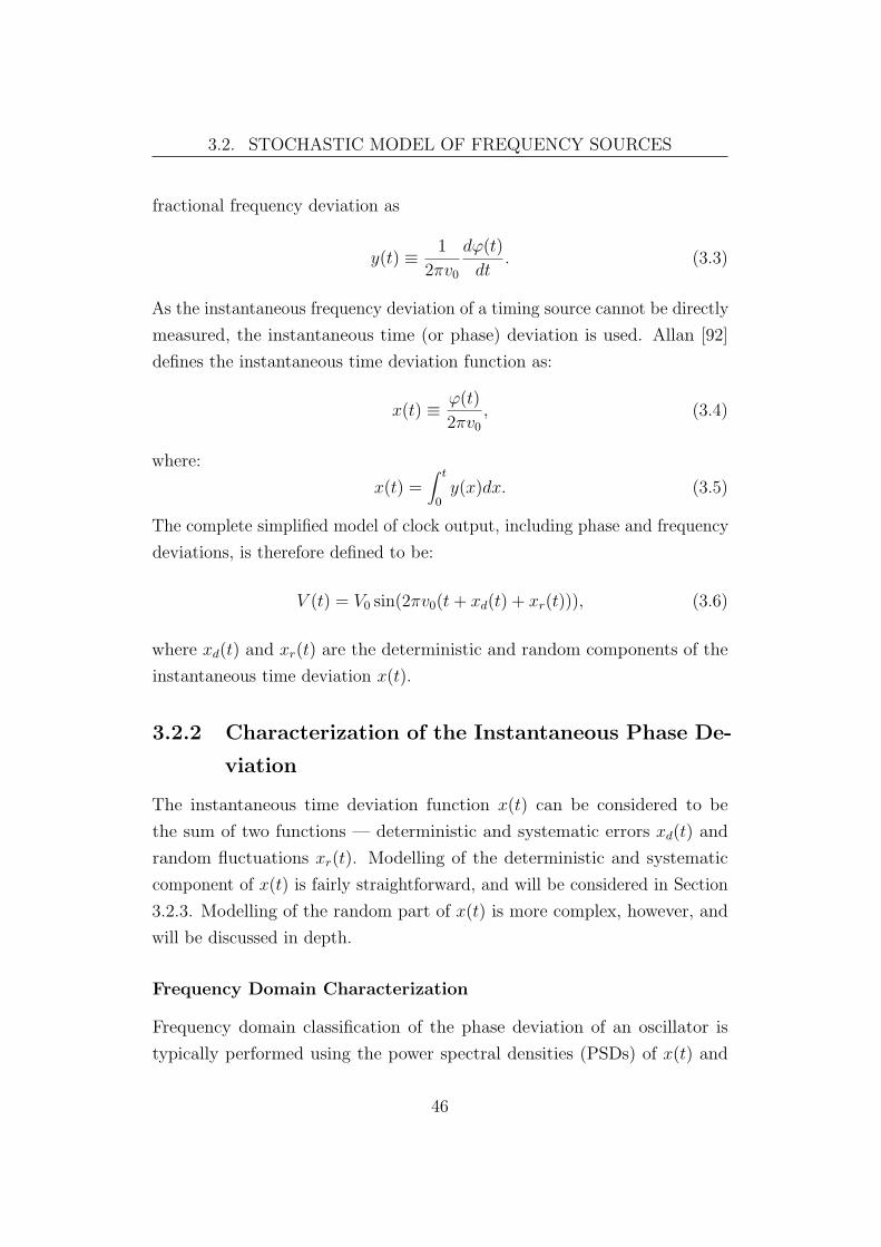
3.2. STOCHASTIC MODEL OF FREQUENCY SOURCES
fractional frequency deviation as
y(t) ≡ 1
2πv0
dϕ(t)
dt. (3.3)
As the instantaneous frequency deviation of a timing source cannot be directly
measured, the instantaneous time (or phase) deviation is used. Allan [92]
defines the instantaneous time deviation function as:
x(t) ≡ ϕ(t)
2πv0
, (3.4)
where:
x(t) =∫ t
0y(x)dx. (3.5)
The complete simplified model of clock output, including phase and frequency
deviations, is therefore defined to be:
V (t) = V0 sin(2πv0(t+ xd(t) + xr(t))), (3.6)
where xd(t) and xr(t) are the deterministic and random components of the
instantaneous time deviation x(t).
3.2.2 Characterization of the Instantaneous Phase De-
viation
The instantaneous time deviation function x(t) can be considered to be
the sum of two functions — deterministic and systematic errors xd(t) and
random fluctuations xr(t). Modelling of the deterministic and systematic
component of x(t) is fairly straightforward, and will be considered in Section
3.2.3. Modelling of the random part of x(t) is more complex, however, and
will be discussed in depth.
Frequency Domain Characterization
Frequency domain classification of the phase deviation of an oscillator is
typically performed using the power spectral densities (PSDs) of x(t) and
46

3.2. STOCHASTIC MODEL OF FREQUENCY SOURCES
y(t), denoted as Sx(f) and Sy(f). For many types of precision oscillators,
Sy(f) can be approximated by a power law model [91]:
Sy(f) =∑
hαfα Hz2/Hz, (3.7)
where fα is the noise category, and hα is the intensity coefficient in that
category. From equations 3.5 and 3.7, the PSD of x(t) can be written [93] as:
Sx(f) =Sy(f)
(2πf)2=∑ hα
4π2fα−2 (3.8)
Five categories of noise, corresponding to integer values of α in equation
3.7, are typically used for the analysis of phase deviation in the frequency
domain. These categories are white phase modulation (α = 2), flicker phase
modulation (α = 1), white frequency modulation (α = 0), flicker frequency
modulation (α = −1) and random walk frequency modulation (α = −2).
Figure 3.4 on page 49 shows examples of x(t) for each noise category.
Considering only the noise categories typically found in frequency sources
[94, 95, 89], a complete frequency domain noise measure can be expressed as:
Sx(f) =2∑
α=−2
hα4π2
fα−2 (3.9)
The phase noise figure L(f) is typically specified on the data sheets of
precision oscillators. The definition of L(f) [96, 97] is:
L(f) = 10 log10(1
2Sx(f)) dBc/Hz. (3.10)
Some devices specify the complete curve of L(f), and some specify only values
of L(f) at certain offset frequencies. L(f) is the IEEE1139-1999 standard [96]
frequency domain measure of oscillator stability. Figure 3.3 illustrates L(f)
specifications for two quartz crystal oscillators — a Wenzel oven controlled
crystal oscillator (OCXO) [98], and a low cost Maxim temperature compen-
sated crystal oscillator (TCXO) [8]. For comparison, requirements of oscillator
phase noise levels for airborne Doppler radars are typically −110dBc/Hz [3]
47
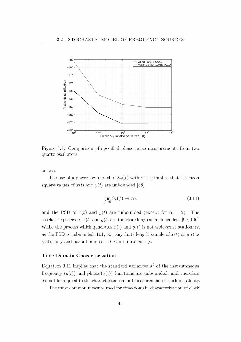
3.2. STOCHASTIC MODEL OF FREQUENCY SOURCES
101
102
103
104
105−180
−170
−160
−150
−140
−130
−120
−110
−100
−90
Frequency Relative to Carrier (Hz)
Pha
se N
oise
(dB
c/H
z)
Wenzel 10MHz OCXOMaxim DS4026 10MHz TCXO
Figure 3.3: Comparison of specified phase noise measurements from twoquartz oscillators
or less.
The use of a power law model of Sx(f) with α < 0 implies that the mean
square values of x(t) and y(t) are unbounded [88]:
limf→0
Sx(f)→∞, (3.11)
and the PSD of x(t) and y(t) are unbounded (except for α = 2). The
stochastic processes x(t) and y(t) are therefore long-range dependent [99, 100].
While the process which generates x(t) and y(t) is not wide-sense stationary,
as the PSD is unbounded [101, 60], any finite length sample of x(t) or y(t) is
stationary and has a bounded PSD and finite energy.
Time Domain Characterization
Equation 3.11 implies that the standard variances σ2 of the instantaneous
frequency (y(t)) and phase (x(t)) functions are unbounded, and therefore
cannot be applied to the characterization and measurement of clock instability.
The most common measure used for time-domain characterization of clock
48
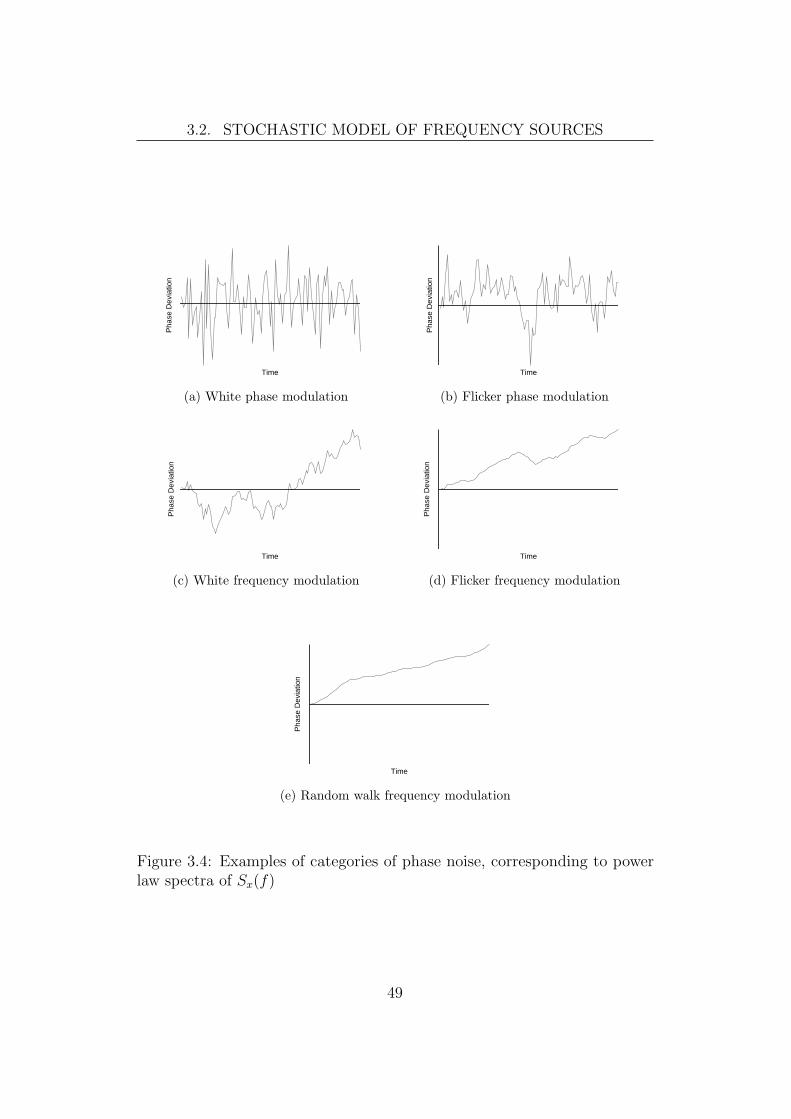
3.2. STOCHASTIC MODEL OF FREQUENCY SOURCES
0 10 20 30 40 50 60 70 80 90 100
−2
−1.5
−1
−0.5
0
0.5
1
1.5
2
Time
Pha
se D
evia
tion
(a) White phase modulation
0 10 20 30 40 50 60 70 80 90 100
−6
−4
−2
0
2
4
6
Time
Pha
se D
evia
tion
(b) Flicker phase modulation
0 10 20 30 40 50 60 70 80 90 100
−8
−6
−4
−2
0
2
4
6
8
Time
Pha
se D
evia
tion
(c) White frequency modulation
0 10 20 30 40 50 60 70 80 90 100
−100
−50
0
50
100
Time
Pha
se D
evia
tion
(d) Flicker frequency modulation
0 10 20 30 40 50 60 70 80 90 100
−250
−200
−150
−100
−50
0
50
100
150
200
250
Time
Pha
se D
evia
tion
(e) Random walk frequency modulation
Figure 3.4: Examples of categories of phase noise, corresponding to powerlaw spectra of Sx(f)
49

3.2. STOCHASTIC MODEL OF FREQUENCY SOURCES
instability is the two-sample, or Allan, variance. In discrete sampled systems,
the two-sample variance is defined as the dimensionless number [102, 103]
σ2y(τ) = lim
N→∞
1
N
N∑n=1
(xn − 2xn−1 + xn−2)2
2τ 2(3.12)
where xn = x(nτ0) and τ0 is the system sample rate. Where only finite
numbers of data points are available, the Allan variance can be estimated as
σ2y(τ) =
1
N − 2m
N−2∑n=1
(xn+2m − 2xn+m + xn)2
2m2τ 20
, (3.13)
where τ = mτ0, τ0 is the system sample rate, and N data points are available.
In bandlimited systems, the Allan variance is known to converge for all
α > −3.
The Allan variance is useful for characterization of noise as σ2y(τ) ∼ τ−α−1
for −3 < α ≤ 1 [104]. Thus, the Allan variance can be used to estimate both
the intensity and power spectral density of noise.
The characterization power of the Allan variance is limited by an ambiguity
where α ≥ 1 — it cannot differentiate between white phase modulation (PM)
and flicker PM noise. This shortcoming is addressed by the modified Allan
variance [104], which is defined as:
Mod σ2y(τ) =
1
2τ 2
⟨(1
n
n∑i=1
(xi+2n − 2xi+n + xi)
)2⟩, (3.14)
where τ = nτ0 and 〈x〉 is the infinite ensemble average of x. For a finite data
set of N points, Mod σ2y(τ) can be estimated as:
Mod σ2y(τ) =
1
2τ 2n2(N − 3n+ 1)
N−3n+1∑j=1
n+j−1∑i=j
(xi+2n − 2xi+n + xi)
2
.
(3.15)
For the modified Allan variance, Mod σ2y(τ) ∼ τ−α−1 for −3 < α < 3.
The modified Allan variance can therefore be used to characterize any of the
five common types of noise, but at a greater computational cost than the
50

3.2. STOCHASTIC MODEL OF FREQUENCY SOURCES
Allan variance.
For long averaging times the total variance measure [105, 106] is a superior
measure of oscillator statistics than estimates of the Allan variance (equation
3.13) . The definition of this measure is similar to the Allan variance, but
operates on a synthetically lengthened sample sequence:
Totvar(τ) =1
2τ 2(N − 2)
N−1∑n=2
(x#n−m − 2x#
n + x#n+m
)2. (3.16)
For n = 1 to N , x#n = xn and for j = 1 to N − 2, x#
1−j = 2x1 − x1+j, and
x#N+j = 2xN − xN−j.
For Totvar(τ), white and flicker phase modulations produce slopes of
τ−1; white frequency modulation (FM), flicker FM and random walk FM
correspond to τ−12 , τ 0 and τ
12 , respectively [105].
Relationship Between Time and Frequency Measures
An integral relationship exists between the PSD and the Allan variance
[94, 107]:
σ2y(τ) =
8
τ 2
∫ ∞0
Sx(f) sin4(πτf)df, (3.17)
however, this relationship is not easily calculated. Simplification of this
relationship can be performed using the model expressed in equation 3.9. The
contribution of each term in the summation can be considered independently,
greatly simplifying the calculation of σ2y(τ) from Sy(f) or Sx(f). The con-
tribution of each term is presented in the following table (from [90]), where
fh is the upper frequency limit of the measurement system, and γ is the
Euler-Mascheroni constant (γ ' 0.57722).
Noise Category Contribution to σ2y(τ)
White PM h23fh
(2π)2τ2
Flicker PM h1
(2π)2τ2 (3 [γ + ln(2πfhτ)]− ln(2))
White FM h0
2|τ |−1
Flicker FM 2h−1 ln(2)
Random Walk FM h−2
6(2π)2|τ |
51

3.2. STOCHASTIC MODEL OF FREQUENCY SOURCES
The Allan variance σ2y(τ) can’t be unambiguously mapped onto Sx(f) (or
Sy(f)), even for −3 < α ≤ 1. Greenhall [107] examines the limitations on the
mapping of the Allan variance onto Sx(f). Due to this limitation, it is more
convenient to specify a simulation model of stochastic oscillator behaviour in
terms of the unambiguous PSDs Sx(f) or Sy(f), than the Allan variance.
3.2.3 Modelling of Deterministic Phase Deviation
Many common types of oscillators exhibit systematic and deterministic devia-
tions from the expected phase in addition to the stochastic phase deviation.
When applying simplified models (such as equation 3.9) to the random part of
the phase deviation, accuracy can be improved by considering deterministic
errors separately.
Environmental Effects
A key source of systematic errors on frequency source outputs is environmental
factors. A large number of such factors exist, including ambient temperature,
vibration, power supply noise, radio frequency (RF) noise picked up from
the environment, vibrations and many others. Many of these factors are
strongly periodic — such as 100Hz for power supply noise, and daily and
yearly periods for temperature effects.
Periodic environmental effects can be added to the frequency domain
model of phase deviation. Considering each environmental factor i to have
amplitude ai and period Ti, then the equation 3.7 can be modified to include
periodic environmental factors:
Sy(f) =∑α
hαfα +
∑i
ai1
Ti. (3.18)
Similarly, periodic environmental factors can be included in the instanta-
neous phase deviation (equation 3.5) as periodic components:
xd(t) ≡1
v0
∑i
(ait sin
(2πt
1
Ti
))(3.19)
52

3.2. STOCHASTIC MODEL OF FREQUENCY SOURCES
Offsets, Drift and Aging
In addition to periodic effects, frequency sources often exhibit other determin-
istic behaviours, such as a constant frequency offset, linear drift, and aging
related behaviours.
Offset is a systematic inaccuracy in the output frequency of an oscillator,
which does not effect the precision of the oscillator and drift is the time
dependent systematic change in frequency of an oscillator [4]. Combining
drift with a frequency offset yields the drift function d(t), which is included
in the oscillator model (equation 3.2) as follows:
V (t) = (V0 + ε(t)) sin (2π(v0 + d(t))t+ ϕ(t)) + V1(t). (3.20)
Considering only linear drift and constant offset allows the definition of
the drift function as d(t) = ∆v + vdriftt, where ∆t is the frequency offset and
vdrift is the frequency drift per unit time. Using this definition, drift and
offset can be included in the definition of instantaneous frequency deviation
(equation 3.3) to form:
y(t) ≡ 1
v0
(∆v + vdriftt+
1
2π
dϕ(t)
dt
). (3.21)
Combining the offset and drift factors with the periodic components of
xd(t) (equation 3.19) yields:
xd(t) ≡1
v0
(∆vt+ vdriftt
2 +∑i
(ait sin
(2πt
1
Ti
))). (3.22)
3.2.4 Timing Jitter
When considering a digital waveform, jitter is the short-term variation in the
timing of significant events (such as edges), compared to the ideal timing
of these events [5]. In this definition, short-term is commonly considered to
refer to events with a frequency greater than 10Hz [108]. Jitter is typically
measured in one of three ways, as illustrated in figure 3.5: period jitter, cycle
to cycle jitter and time interval error (TIE). Period jitter is the random
53

3.2. STOCHASTIC MODEL OF FREQUENCY SOURCES
Figure 3.5: Definition of Period Jitter and Time Interval Error (after [5])
deviation of the length of each period of the waveform, cycle to cycle jitter
is the random deviation in the length of each pair of adjacent cycles, and
time interval error is the deviation of the position of edges from their ideal
positions. Period jitter sample N is related to cycle to cycle jitter sample N
by:
CN = PN − PN−1 (3.23)
and to the TIE at period N by:
TIEN =N∑i=0
(PN − Pideal) , (3.24)
where Pideal is the ideal period.
The jitter on a digital clock signal derived from an oscillator with phase
noise can be calculated by integrating the phase noise spectrum over the
frequency band of interest [109]. Typically, the lowest frequency of interest is
10Hz, and the highest frequency of interest is 2f0, where f0 is the oscillator
frequency [110]. From the definition of L(f) (equation 3.10), the time interval
error noise power can be estimated by:
J =∫ 2f0Hz
10HzL(f)df. (3.25)
54

3.3. GENERATION OF SYNTHETIC PHASE NOISE SEQUENCES
The estimated RMS jitter is therefore [110]:
JRMS =
√2√
10J/10
2πf0
seconds. (3.26)
3.3 Generation of Synthetic Phase Noise Se-
quences
Generation of synthetic clock signals for computer simulation requires calcula-
tion of the deterministic phase deviation xd(t), and generation of a synthetic
noise sequence matching the statistical properties of the random phase devia-
tion xr(t).
Calculation of xd(t) is straightforward, and can be performed directly
using equation 3.22. The synthesis of xr(t) matching the required PSD and
statistical properties is more complex, especially where large numbers of
samples are required.
For computer simulation, a discrete representation of xr(t), which will be
called xr[n], must be used. In this model, xr[n] will be considered a discrete
representation of a version of xr(t) strictly bandlimited to f02
Hz, where f0 is
the system sample frequency. Using a strictly bandlimited xr(t) allows the
model to ignore the effects of aliasing [102] of the higher frequency components
of xr(t) on the spectral density of xn[t].
3.3.1 Power Law Noise Model
Equation 3.8 defines a power-law PSD model for xr(t). An explicit distinction
must be made between random numbers with a power law distribution (that
is, a probability density function (PDF) of the form p(x) ∝ x−α), and random
numbers with a power law power spectral density (such as those defined by
equation 3.8) — this section is concerned with the latter. To avoid confusion,
we will refer to the noise types of interest as 1/f noise, for all α.
55

3.3. GENERATION OF SYNTHETIC PHASE NOISE SEQUENCES
3.3.2 Autocorrelation
The discrete Einstein-Wiener-Khinchine [111, 60] theorem relates the auto-
correlation sequence φxx[n] of the samples x[n] to the PSD Sx[f ] of those
samples:
φxx[n] =1
N
N−1∑f=0
Sx[f ] exp(
1
n2jπfN
)(3.27)
By the localisation property of the discrete Fourier transform [29], the auto-
correlation φxx[n] tends to spread as the PSD Sx[f ] becomes more compact.
Following this observation, it is clear that for noise matching the PSD in
equation 3.8 will have a wide spread autocorrelation where α ≤ 1 due to the
strongly compact nature of the PSD. As x(f) is long-range dependent [100]
(see Section 3.2.2),∞∑n=1
|φxx[n]| =∞. (3.28)
Categorising phase noise as a long-range dependent process adds the
requirement of a long memory to processes which produce noise of this type.
Long-term autocorrelation also implies that phase noise correlations may exist
between radar pulses — these correlations must be preserved for accurate
simulation.
3.3.3 Existing Approaches to 1/f Synthesis
Techniques for the digital synthesis of 1/f noise samples are well described
in literature. Available techniques can be divided into two categories: exact
and inexact. Exact generation techniques, where no systematic deviation is
allowed from the required spectrum, include fast Fourier transform (FFT)
based methods [112, 113] and time-domain filtering of discrete Poisson events
[114]. Inexact synthesis methods, where some ripple or error is permissible
in the noise PSD, include cascaded infinite impulse response (IIR) filters
[115], cellular automata [116], iterated function systems [117], truncated
autoregressive (AR) filters [113], Wavelets [118, 119, 120] and others.
The requirements for noise synthesis for radar simulation include the ability
to generate noise sequences for all 2 ≤ α ≤ −2, computational efficiency,
56

3.3. GENERATION OF SYNTHETIC PHASE NOISE SEQUENCES
memory efficiency and accuracy. Radar simulations require large volumes of
random samples to be generated, and algorithms must be chosen which are
suitable for this use.
3.3.4 Synthesis Using Time Domain Filtering
In general, it is not possible to filter a sequence of samples using a finite
length digital filter to produce an exact 1/f response [113]. It is not possible,
therefore, to apply a filter of shorter than N samples to produce the desired
N samples of the 1/f noise process.
The processing of N samples with an N tap filter can be performed in
O(N logN) time, using the FFT [112, 113] provided N is known. If N is
not known, filtering must be performed in the time domain, requiring O(N2)
operations and O(N) memory. For large radar simulation problems, the
requirement of O(N) memory for N noise samples is likely to be restrictive,
and alternate approaches which do not require storage of all noise samples
must be sought.
In the generation of noise for radar simulation some ripple, provided it is
sufficiently small, can be allowed in the 1/f PSD of the generated samples.
Relaxing the requirement for exact synthesis allows implementation of time
domain filtering with filters shorter than N .
Truncation of Exact Filters
The transfer function of an ideal filter for the generation of 1/f noise is [121]:
H(z) =1
(1− z−1)(−α+2)/2. (3.29)
From this relation, it is clear that trivial filters can be derived using the
inverse z-transform [29] for α = 2, α = 0 and α = −2. For α = 0, the
required filter is an ideal integrator, and for α = −2 it is a cascade of two
ideal integrators.
Where α does not take on one of these convenient values, the M co-
efficients for an exact autoregressive (AR) filter for M = N can be derived
57

3.3. GENERATION OF SYNTHETIC PHASE NOISE SEQUENCES
10−4
10−3
10−2
10−1−2
0
2
4
6
8
10
Normalized Frequency
Err
or (
dB)
1000 Samples100 Samples
Figure 3.6: Deviation of truncated filters from the target response for N = 105
and α = 1 (from [6])
from equation 3.29 [113]:
a0 = 1 and
ak =(k − 1− −α + 2
2
)ak−1
k. (3.30)
An approximation of the exact roll-off is produced where M < N . The PSD
of the noise generated using such a truncated filter matches the required
slopes at high frequencies but has a flat spectrum at low frequencies. The
roll-off between the required slopes and flat response depends on M and α
[6], but occurs at approximately ω = 2πM
.
Figure 3.6 illustrates the deviation from the required response for two
truncated filters for α = 1 generated using equation 3.30. Errors are well
constrained for ω > 2πM
, but increase at approximately 3dB per octave at
lower frequencies.
While equation 3.30 produces ideal filters for M = N , the filters produced
for M < N do not produce optimal results for a filter of length M . For
example, a numerically designed third order IIR filter for α = 1 (due to
Bristow-Johnson [122]) can match the required roll-off within 0.3dB over ten
58

3.3. GENERATION OF SYNTHETIC PHASE NOISE SEQUENCES
10−3
10−2
10−1−5
−4
−3
−2
−1
0
1
2
Frequency (Normalized to fs =1)
Dev
iatio
n fr
om f−
1 res
pons
e (d
B)
IIR Filter (Order 3)AR Filter (Order 100)
Figure 3.7: Comparison of deviations from the exact response of an optimalIIR filter, and an AR filter designed using equation 3.30 (from [6])
octaves [122]. Figure 3.7 compares a hand designed order three filter for α = 1
with an order 100 filter designed using equation 3.30.
Filter Design Using Optimization Techniques
A variety of optimisation based design techniques exist, aimed at the direct
design of digital (both finite impulse response (FIR) and IIR) filters approach-
ing a desired response. These approaches can be divided into two categories:
least-squares optimisation, and Chebyshev optimisation.
Least-squares optimisation approaches aim to design a filter with a chosen
number of coefficients which approaches the target response in the least
squares sense. That is, they aim to find a rational transfer function H(z)
which minimises the value of S, where
S =1
2π
∫ 2π
0
(Ht(e
jω)−H(ejω))2dω, (3.31)
and Ht(z) is the desired transfer function. One optimisation method of
59

3.3. GENERATION OF SYNTHETIC PHASE NOISE SEQUENCES
10−5
10−4
10−3
10−2
10−1
100−5
0
5
10
15
20
25
30
Normalized Frequency
Err
or (
dB)
Least−squares Optimised FilterTruncated Ideal Filter
Figure 3.8: Comparison of deviation from α = 1 response for least-squaresoptimal filter and truncated ideal filter (order = 30)
this kind, the modified Yule-Walker [123] method, is very widely used and
implemented.
Despite its wide applicability to filter design problems, least squares opti-
misation is not suited to finding filters with 1/f type responses. Optimisation
of S (equation 3.31) will find filters which closely match the required response
for high frequencies, but like the truncated ideal filters, they do not match
the required roll-off at low frequencies. This is because the width of the low
frequency error is fairly low, and it has less effect on least-squares error than
ripple at higher frequencies. Figure 3.8 compares the performance of an order
30 filter designed using the Yule-Walker least-squares optimisation procedure,
and the order 30 truncation of the ideal filter for α = 1. In this case, the
least-squares designed filter performs better than the truncated filter at high
frequencies.
Filter design using Chebyshev norm optimisation (also known as minimax
optimisation and l∞ optimisation) seeks to find the rational transfer function
H(z) which minimizes [124]
‖H(ejω)−Ht(eω)‖ = max
0≤ω≤2π|H(ejω)−Ht(e
jω)|, (3.32)
60

3.4. MULTIRATE FILTERS AND NOISE GENERATION
where Ht(z) is the required transfer function. That is, this procedure seeks
to find the filter which minimizes the maximum deviation, at the cost of
increased least-squares error [125].
Chebyshev optimal filter design is not as widely used as least-squares
filter design, but has been extensively developed for cases where minimax
optimisation is required. Available algorithms for Chebyshev optimisation
include those based linear programming [126, 127], linear programming with
differential correction [128, 129], the rational Remez exchange algorithm [124],
eigenvalue decomposition [130, 131], and others.
Time domain filtering approaches are suitable for the efficient approxi-
mation of 1/f noise sequences for radar simulation. The design of filters for
odd (and non-integer) α is challenging, and requires compromise between
filter length, minimax error and least-squares error. Chebyshev optimal filters
reduce error close to the carrier, but tend to introduce unacceptable deviations
from the required response at higher frequencies. Least-squares optimal and
truncated ideal filters match the required roll-off closely at high frequencies,
at the cost of a flat response at low frequencies and truncation of the noise
autocorrelation sequence.
3.4 Multirate Filters and Noise Generation
The time domain filtering technique is the most promising for the generation
of synthetic phase noise sequences for radar simulation. The shortcomings of
this technique, namely the difficulty of filter design and truncation of auto-
correlation sequences, can be addressed by using multirate signal processing
techniques.
3.4.1 Overview of Multirate Signal Processing
Multirate signal processing refers to digital signal processing performed with
a set of operations including the compression and expansion operations, in
addition to the operations used in single rate digital signal processing (DSP)
[29]. The compression (also widely referred to as decimation) operation,
61

3.4. MULTIRATE FILTERS AND NOISE GENERATION
typically written as ↓ k for integer k, corresponds to the creation of a signal
which contains every kth sample of the original signal [132, 133]. Where y[m]
is x[n] compressed by the factor k,
y[m] = x[nk]. (3.33)
The expansion operation, typically written as ↑ k for integer k, corresponds to
the creation of a signal, every kth sample of which is a sample of the original
signal [132], and the rest are zero. Where y[n] is x[n] expanded by the factor
k,
y[m] =
x[mk
] mk∈ Z,
0 otherwise.(3.34)
The upsampling operation is related to the expansion operation, by the
use of a suitable filter for rejecting the images of x[n] in the frequency
domain introduced by expansion. The downsampling operation is related
to compression, by the use of a suitable anti-aliasing filter to remove all
frequencies of x[n] above 1k
times the sampling rate of x[n]. The resampling
operation by the rational factor ab
corresponds to upsampling by a, followed
by downsampling by b.
3.4.2 Multirate Filterbanks for 1/f Noise
Examination of figure 3.8 on page 60 reveals that the least-squares optimal
filter for α = 1 designed using the modified Yule-Walker [123] algorithm
closely matches the required response over the top decade of frequency (that
is, from 12fs to 1
10fs). Figure 3.9 shows that the maximum deviation from the
required response in this range for an order 10 least-squares IIR filter is less
than 0.05dB.
Based on the observation that standard filter design procedures can
accurately match the required response over a single decade of frequency, it
can be hypothesised that a filter Y (ω) exists with similarly low ripple, made
up of filters Gi(ω) which match the required roll-off in the ith decade and
62
3.4. MULTIRATE FILTERS AND NOISE GENERATION
10−1
100−0.05
−0.04
−0.03
−0.02
−0.01
0
0.01
0.02
Normalized Frequency
Err
or (
dB)
Figure 3.9: Deviation from α = 1 response for least-squares optimal filterover the top decade of frequency (order = 10)
ideal bandpass filters Bi(ω), which select that decade:
Y (ω) =∞∑i=1
Bi(ω)Gi(ω). (3.35)
Such a filter would not be practically realizable, as it requires an infinite
sequence of subfilters and ideal bandpass filters. The decades of frequency
below a particular limit can be discarded, as radar simulations are unlikely
to be interested in phase noise periods in the order of centuries. Selecting D
decades of frequency:
Y (ω) =D∑i=1
Bi(ω)Gi(ω). (3.36)
Y (ω) could be physically realised using the structure shown in figure
3.10. In this structure y[n] are the simulated phase noise samples, and
g[n] are independent white Gaussian noise samples. Simplification of this
structure, and application of multirate signal processing techniques, allows
an approximation to the ideal filter Y (ω) to be implemented computationally
efficiently.
63

3.4. MULTIRATE FILTERS AND NOISE GENERATION
Figure 3.10: Filter structure for Y (ω)
Figure 3.11: Simple multirate implementation of filter structure for Y (ω)
Multirate Implementation of Y (ω)
The ideal time-domain noise filter Y (ω) is ideally suited to implementation as
a multirate filterbank. The top subband B0(ω) G0(ω) has only slightly less
bandwidth than the whole system, so it must be run at the system sample
rate f0. The next subband has ten times less bandwith, and therefore can be
run at a tenth of the sample rate and so on. In addition, the ideal bandpass
filter Bi(w) can be divided into two sections, a lowpass Li(ω) and a highpass
Hi(ω).
Executing each branch of the filter structure (figure 3.10) at sample rate
suitable for its bandwidth has several advantages. If branches are spaced
decades of frequency apart, and the sample rate in each branch is ten times
lower than the next branch up, the same filters G(ω) and B(ω) can be used
in each branch.
Figure 3.11 illustrates a simple adaptation of the structure in figure 3.10
64

3.4. MULTIRATE FILTERS AND NOISE GENERATION
Figure 3.12: Optimised multirate implementation of filter structure for Y (ω)(Adapted from Park et. al. [7])
to use multirate signal processing principles. In this figure ↑ N corresponds
to expansion by a factor of N , and Li(ω) in an anti-imaging (interpolation)
filter suitable for the upsampling operation. This structure can be further
re-arranged to increase efficiency [7] by reducing the number of filtering
operations required in each branch and the number of operations performed
at the full rate.
Figure 3.12 illustrates an optimised structure for the implementation of
Y (ω). In this structure, the bandpass filter B(ω) has been divided into
highpass (H(ω)) and lowpass (L(ω)) sections. The lowpass sections have
been combined with the anti-imaging (interpolation) filters for each branch,
reducing the number of filtering operations required. In addition, the filters
used for each branch are identical — only one set of filter designs is required.
For optimal performance of the structure in figure 3.12, the filters H(ω) and
L(ω) must have narrow transition bandwidths, adequate stopband attenuation,
and a flat (within reasonable bounds) summed response. The design of pairs
of filters with the required specifications is well understood [133, 132] and can
65

3.4. MULTIRATE FILTERS AND NOISE GENERATION
Figure 3.13: A single branch of the optimised multirate filter structure forY (ω)
be performed with standard filter design techniques. Elliptic [29, 134] filters
are ideal for this purpose, as ripple can be tolerated in both the passband
and stopband.
3.4.3 Computational Efficiency
The computational requirements of a single branch (figure 3.13) of the mul-
tirate filter structure for noise generation (figure 3.12) can be computed by
adding up the individual computational requirements of each element. The
branch includes two filters operating at the branch’s sample rate, and one
at ten times that rate. The summation and upsampling operations are also
included.
Assuming that the three filters G(ω), H(ω) and L(ω) are implemented
as direct form II [29] IIR filters with order N , each sample passed through
these filters will require 2N + 1 multiplications, 2N additions and N memory
slots [27]. The filter L(ω) is clocked at ten times the rate, and hence will
require 20N + 10 multiplications and 20N additions for each noise sample
produced by the branch. Expansion is a simple padding operation, and does
not require any calculations. The total number of calculations for C required
for each branch is C = 4NG + 4NH + 40NL + 12 for each sample, where NG,
NH and NL are the orders of G(ω), H(ω) and L(ω) respectively. The highest
rate branch does not require L(ω), and hence requires C = 4NG + 4NH + 2
calculations.
For each sample produced by the complete structure with D branches,
66

3.4. MULTIRATE FILTERS AND NOISE GENERATION
the number of calculations required is
Ct = 4
(NG +NH +
D∑i=1
1
10i(NG +NH + 10NL + 12)
). (3.37)
Choosing N = maxNH , NG, NL, the upper bound of
Cu = 4
(2N + (12N + 13)
D∑i=1
1
10i
)=
1
9(120N + 48) (3.38)
is set.
If a single IIR filter with the required response and order M were
to exist, producing each sample with such a filter would require 2M + 1
calculations. The multirate filter bank is therefore more efficient when
M > 118
(120N + 48) + 1. For example, for N = 30 the multirate struc-
ture is more efficient where M ≥ 204 — and, as Section 3.3.4 discusses, no
filter with such a short length is possible for most values of α over more than
a few decades of frequency.
3.4.4 Accuracy
The accuracy of fit of the PSD of the noise generated using the multirate
approach depends on the performance of the filters in the multirate filterbank.
Specifically, the accuracy of the slope of the generated noise PSD depends on
how well G(ω) matches the required slopes over the top decade of frequency.
Deviations from perfect reconstruction in the filter pair H(ω) and L(ω) will
cause ripple on decade boundaries. Passband ripple on H(ω) and L(ω) will
produce ripple on the produced PSD, and insufficient stopband attenuation
in these filters will allow the behaviour of G(ω) outside the band of interest
to reduce the accuracy of the required estimate.
Figure 3.14 shows the performance of the filterbank for various α, estimated
using the FFT and averaged over 100 runs to reduce the variance. For G(ω), an
11th order IIR filter designed using the modified Yule-Walker [123] algorithm
was used. For H(ω) and L(ω), a pair of 11th order Elliptic (Cauer) filters
[135, 27] was used.
67

3.4. MULTIRATE FILTERS AND NOISE GENERATION
10−5
10−4
10−3
10−2
10−1
100
−90
−80
−70
−60
−50
−40
−30
−20
−10
0
10
Normalized Frequency
Noi
se P
ower
(dB
)
Measured PSDIdeal PSD
(a) α = 0
10−5
10−4
10−3
10−2
10−1
100
−50
−40
−30
−20
−10
0
10
Normalized Frequency
Noi
se P
ower
(dB
)
Measured PSDIdeal PSD
(b) α = 1
Figure 3.14: Comparison of generated noise PSD versus required PSD fortwo coloured pseudonoise sequences
68

3.5. PHASE NOISE GENERATION USING MULTIRATE FILTERS
Figure 3.15: Piecewise linear representation of the power law noise model
3.5 Phase Noise Generation Using Multirate
Filters
The multirate filtering procedure for generation of coloured noise sequences
described in Section 3.4 on page 61 is well suited to the generation of synthetic
phase noise sequences for radar simulation. The procedure, as presented, is
suitable to the generation of coloured noise for a single value of α, generaliza-
tions to the procedure can be made to allow the generation of noise sequences
matching the model presented in equation 3.8.
3.5.1 Polynomial Model of the Noise Spectrum
Where Sx(f) matches the power law noise model (equation 3.9), it can
be represented as a linear combination of powers of f−1 [102, 136], which
corresponds to a strictly decreasing upwardly concave curve on a log-log scale.
Figure 3.15 illustrates such a model, where noise of each category dominates
over some part of the spectrum. The positions of the breakpoints in the linear
piecewise model of the noise PSD depend on the values of hα for each noise
category of interest.
For each noise category α, hα must be chosen to obtain a least-squares fit
between the modelled PSD and the measured instantaneous phase deviation
69
3.5. PHASE NOISE GENERATION USING MULTIRATE FILTERS
PSD of the device to be simulated. That is,
Error =∫ fs
2
0
2∑α=−2
(hα4π2
f−α)− Smx (f)
2
df, (3.39)
must be minimised, where Smx (f) is the instantaneous phase deviation PSD
of the measured oscillator. Methods for the extraction of hα from measured
data depend on the type of measurements available. Widely used techniques
include extraction from the Allan variance or modified Allan variance (Section
3.2.2), the lag 1 autocorrelation technique [137] and least squares polynomial
fitting. Direct least-squares polynomial fitting of Smx (f) is not possible, but
hα for −2 ≤ α ≤ 2 can be extracted from a fourth order polynomial fit to
f 4Sxm(f).
In order to perform this direct fitting, the spectrum of the phase noise
must be estimated from a limited number of samples. The periodogram, the
FFT of the samples with the application of a suitable window, has two major
disadvantages for the estimation of power-law spectra [138]: high variance,
and the effects of spectral leakage. High variance reduces the accuracy of
a polynomial fit to the spectrum, and spectral leakage causes errors in the
slope of the spectrum estimate where α < 0.
Austin et. al. [138] recommend Capon’s estimator [139] as particularly
well suited to the estimation of power-law spectra. Other suitable techniques
include the widely used Welch [140] modified periodogram method, and a
variety of methods based on wavelets ([120] and [119], for example). An
extensive discussion of spectral estimation procedures can be found in Kay
[141].
The power law model (equation 3.9) can be directly implemented using
a multirate filterbank to generate noise independently for each value of α.
Efficiency can be increased, however, by only calculating each noise type over
the decades of frequency where that noise type dominates. For example, if
α = 0 noise dominates Sx(f) for some of the second and third highest decades
of frequency, only those branches of the multirate filterbank corresponding to
that frequency range need to be calculated. As some overlap is required for
70

3.5. PHASE NOISE GENERATION USING MULTIRATE FILTERS
Figure 3.16: Modified multirate filter structure for the efficient generation ofnoise matching a spectrum polynomial in f−1 (from Brooker et. al. [6])
accuracy, and as frequency breakpoints are unlikely to be situated on decade
boundaries, care must be taken to remove only those branches which will
have an insignificant effect on the total noise PSD.
3.5.2 Phase Noise Generation Example
Figure 3.17 illustrates the result of the application of the piecewise noise
generation model to the synthesis of phase noise matching the specifications
of the MAXIM DS4026, a 10MHz TCXO [8]. A polynomial representation of
Sx(f) for −2 ≤ α ≤ 2 (equation 3.9) was fitted to the specified characteristic
phase noise PSD of the oscillator. The least-squares fit, figure 3.17(a), was
found to match the specified phase noise curve within 4dBc/Hz between 10Hz
and 1MHz from the carrier.
An implementation of the multirate filterbank, figure 3.12, was used to
generate coloured noise for each α, which were scaled with hα derived from
the polynomial fit. Figure 3.17(b) compares the PSD of 106 generated samples
and the target PSD. The generated noise closely matches the required PSD
71

3.5. PHASE NOISE GENERATION USING MULTIRATE FILTERS
101
102
103
104
105
106
−160
−150
−140
−130
−120
−110
−100
−90
Frequency (Hz)
Pha
se N
oise
(dB
c/H
z)
Polynomial FitSpecified Phase Noise
(a) Least-squares polynomial fit to specified phase noise curve
101
102
103
104
105
−200
−190
−180
−170
−160
−150
−140
−130
−120
−110
−100
−90
Frequency (Hz)
Pha
se N
oise
(dB
c/H
z)
(b) Comparison of PSD of generated phase noise and target polynomial
Figure 3.17: Results of synthesis of phase noise matching the specifications ofthe Maxim DS4026 10MHz TCXO [8]
72

3.6. EFFICIENT NOISE SYNTHESIS FOR PULSED RADAR
over the entire range of frequencies of interest.
3.6 Efficient Noise Synthesis for Pulsed Radar
For simulations of pulsed radar systems, synthetic phase noise is only required
for simulation during the transmit and receive windows [26, 50]. It is necessary,
however, to conserve the long-term correlations which are inherent in phase
noise, due to the long-memory [100, 142] nature of the generating process. It
is computationally inefficient to generate phase noise samples corresponding
to the times when the simulated radar system is neither transmitting nor
receiving.
The discrete Einstein-Wiener-Khinchin theorem [111, 60] states that the
PSD of a sequence of samples x[n] is equal to the discrete Fourier transform
of the autocorrelation sequence of x[n] [27]. From this observation, and
the localisation property of the Fourier transform, it can be observed that
the low-frequency branches of the multirate structure make the strongest
contribution to the long-term correlations of x[n].
Figure 3.18 illustrates the autocorrelation sequence for a 105 point noise
sequence where α = 0. The autocorrelation sequences of the filtered noise
illustrates the effects of removing branches from the multirate filter. The
autocorrelation of the lowpassed sequence (figure 3.18(b)) corresponds to the
removal of the three highest frequency (and hence highest rate) branches
from the tree. The autocorrelation of the highpassed sequence (figure 3.18(c))
illustrates the change in total autocorrelation due to the removal of these
branches. While the absolute value of the differences is due to the relatively
lower energy in the higher frequency bands, the shape of the high frequency
autocorrelation illustrates that it makes little contribution to the long term
correlation of the noise sequence. This results corresponds to the localisation
property of the PSD — the support of the highpassed sequence is wide,
therefore it has a narrow autocorrelation, conversely the support of the
lowpassed sequence is narrow, and it has a wide autocorrelation. Similar
results are obtained for 1 ≤ α ≤ −2.
73

3.6. EFFICIENT NOISE SYNTHESIS FOR PULSED RADAR
0 0.5 1 1.5 2x 10
5
−2
0
2
4
6
8
10
12x 109
Lag
Aut
ocor
ella
tion
(a) Full spectrum
0 0.5 1 1.5 2x 10
5
−2
0
2
4
6
8
10
12x 109
Lag
Aut
ocor
rela
tion
(b) Lowpass at ω = 2π/1000
0 0.5 1 1.5 2x 10
5
−1
−0.5
0
0.5
1
1.5
2
2.5x 10⁷
Lag
Aut
ocor
rela
tion
(c) Highpass at ω = 2π/1000
Figure 3.18: Autocorrelation of filtered noise sequences for α = 0
74

3.6. EFFICIENT NOISE SYNTHESIS FOR PULSED RADAR
The Dynamic Pruning Approach
The long-term correlations present in 1/f noise sequences can be preserved
while reducing computational costs by dynamically ‘pruning’ the higher
frequency branches from the multirate filterbank during inter-pulse periods.
Assuming H(w) in figure 3.16 is an ideal high pass filter, the nth branch
of the filter bank will decorrelate in approximately 10k
fsseconds. Branches
which decorrelate during the inter pulse interval can be pruned during this
interval without destroying the long-memory nature of the generated sequence.
Pruned branches are flushed and restarted at the end of the interval.
Algorithm 1 Dynamic pruning algorithm
while Phase noise samples are required do
while In the receive/transmit period do
Calculate samples using complete structure
end while
Compute the number of branches that will decorrelate during the inter
pulse interval, K
Disable top K branches from the filter structure
while In the inter pulse period do
Calculate samples using pruned structure
end while
Flush memory of top K branches
Re-enable top K branches
end while
If K of the D branches of the filterbank can be pruned during the interpulse
periods, the number of operations per sample (equation 3.37) is reduced to
Ct = 4 (NG +NH + 10NL = 12)D∑i=K
1
10i(3.40)
The total reduction per branch removed is therefore approximately
Ct =(NG +NH + 10NL = 12)
∑Di=1
110i
(NG +NH + 10NL = 12)∑Di=2
110i
=1
10, (3.41)
75
3.6. EFFICIENT NOISE SYNTHESIS FOR PULSED RADAR
or 90% reduction per branch removed.
Applying the pruning approach to preserving long-term correlations allows
these correlations to be preserved over the inter-pulse interval with low
computational and memory requirements.
Dynamic Pruning Performance Example
The real world performance advantages of the pruned multirate filterbank
approach were measured during the simulations of the pulse-Doppler system
described in Section A.2 on page 133. This simulated system has a PRI of
50µs and a receive window of 2.5µs, for a total receiver duty cycle of 5%. To
compare the performance of the pruned and complete structures, 200× 106
samples were generated using the pruned and complete filterbanks.
The complete structure generated 200 × 106 samples in an average of
6.01s. The Callgrind [143] cache simulator estimated that 2.09× 10¹⁰ CPU
cycles were required on an Intel Core 2 processor. In this example, 95% of
the generated samples were unused. Using the dynamic pruning approach,
the samples were generated in an average of 0.25s, requiring an estimated
1.13 × 10⁹ CPU cycles. This difference in computation time reflects an
reduction in the required computation time by 18.5 times, while preserving
the long-memory nature of the generated noise sequences.
Another example of the advantages of the dynamic pruning algorithm is
present in Section A.2 in Appendix A. In this example, long term phase noise
correlations were preserved over simulation times up to 100 seconds — which
would have required a naive algorithm to generate 100 × 108 phase noise
samples. For the 100s simulation, the dynamic pruning algorithm reduced
the computer time required to generate the phase noise samples by a factor
of 105.
76

3.7. EFFECTS OF OSCILLATOR BEHAVIOUR ON RADAR SIGNALS
3.7 Effects of Oscillator Behaviour On Radar
Signals
3.7.1 Upmixing and Downmixing Effects
The effects of deviations from the ideal behaviour of the receiver (figure 2.13)
and transmitter (figure 2.12) local oscillators can be modelled as a variety of
effects on the complex signal envelope xl[n]. The effects of these deviations
on the performance of radar systems is complex, and highly dependent on the
type of processing used on the received signals. Analyses for moving target
indication (MTI) radar systems, for example, can be found in Shrader and
Gregers-Hansen [144] and Kerr [145].
Deterministic Phase and Frequency Errors
Constant phase errors on the system clock (xd(t) = φ for constant φ in
equation 3.6) is equivalent to a phase shift of the received signal, and is not
distinguishable from the phase shift due to propagation delay (equation 2.28).
Constant frequency offset on the system clock (xd(t) = fet for constant fe in
equation 3.6) is equivalent to a time dependent phase shift on the received
signal. For a single target, this time dependent phase shift is indistinguishable
from the frequency shift caused by a time-dependent change in the target
range — the Doppler effect.
Coherent [146] radar systems seek to reduce these constant deterministic
errors through time and frequency calibration, as coherent operation has many
advantages in both monostatic [147] and multistatic [86, 87] radar systems.
Random Phase and Frequency Errors
Including phase noise on the local oscillators in figure 2.8, an expression for the
complex output y(t), in terms of the input complex signal xl(t), instantaneous
phase deviation on the transmit and receive local oscillators nt(t) and nr(t),
77
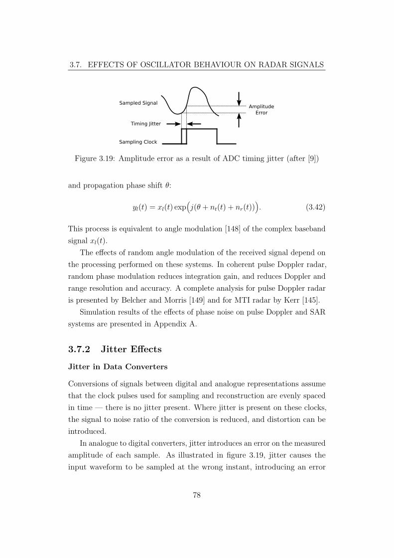
3.7. EFFECTS OF OSCILLATOR BEHAVIOUR ON RADAR SIGNALS
Figure 3.19: Amplitude error as a result of ADC timing jitter (after [9])
and propagation phase shift θ:
yl(t) = xl(t) exp(j(θ + nt(t) + nr(t))
). (3.42)
This process is equivalent to angle modulation [148] of the complex baseband
signal xl(t).
The effects of random angle modulation of the received signal depend on
the processing performed on these systems. In coherent pulse Doppler radar,
random phase modulation reduces integration gain, and reduces Doppler and
range resolution and accuracy. A complete analysis for pulse Doppler radar
is presented by Belcher and Morris [149] and for MTI radar by Kerr [145].
Simulation results of the effects of phase noise on pulse Doppler and SAR
systems are presented in Appendix A.
3.7.2 Jitter Effects
Jitter in Data Converters
Conversions of signals between digital and analogue representations assume
that the clock pulses used for sampling and reconstruction are evenly spaced
in time — there is no jitter present. Where jitter is present on these clocks,
the signal to noise ratio of the conversion is reduced, and distortion can be
introduced.
In analogue to digital converters, jitter introduces an error on the measured
amplitude of each sample. As illustrated in figure 3.19, jitter causes the
input waveform to be sampled at the wrong instant, introducing an error
78

3.7. EFFECTS OF OSCILLATOR BEHAVIOUR ON RADAR SIGNALS
10−12
10−11
10−10
10−9
10−8−50
0
50
100
150
200
250
300
Timing Jitter (s)
SN
R (
dB)
100KHz Bandwidth1MHz Bandwidth100MHz Bandwidth
Figure 3.20: Data converter maximum SNR versus RMS timing jitter
proportional to the slope of the signal between the ideal sampling instant
and the actual sampling instant. Similar effects are present on the output
of digital to analogue converters [150]. In sampling of a single sinusoid of
frequency f0, the maximum SNR of the sampling system is [151]:
SNRmax =1
4π2f 20σ
2t
, (3.43)
where σt is the RMS jitter in seconds. For non-sinusoidal band-limited signals
with bandwidth B and σt 1/B, the maximum signal to noise ratio (SNR)
is approximately [9]:
SNRmax =1
2π2B2σ2t
. (3.44)
Figure 3.20 illustrates the maximum SNR of a data converter in terms
of the bandwidth of the converter and RMS timing jitter. The output SNR
of the sampling process is degraded when the peak amplitude error due to
timing jitter becomes bigger than the quantization step size at the effective
number of bits of the ADC.
79

3.8. CONCLUSION
3.8 Conclusion
A multirate filterbank for the synthesis of coloured noise sequences has been
developed, expanding on the results of Park et. al. [7]. This approach to the
generation of coloured noise offers improved efficiency over methods such as
direct IIR filtering [113], FFT based methods [112], and other widely used
methods.
An investigation into the statistical properties of oscillator phase and
frequency noise has been completed. A polynomial model for the power-
spectral density of oscillator phase noise has been derived, based on a simple
model of oscillator behaviour. This model has been combined with the
multirate filterbank approach to coloured noise generation to create a complete
algorithm for the generation of synthetic clock phase noise sequences, matching
measured or specified oscillator performance parameters. Algorithms for the
generation of sparse or pulsed sequences of synthetic oscillator phase noise
samples have also been developed.
The multirate approach to the generation of synthetic phase noise se-
quences matching a specified PSD is believed to be novel, and an original
contribution to the field. The application of pruning of multirate filterbanks
to the generation of sparse coloured noise sequences is also believed to be
novel.
80

Chapter 4
Simulator Development and
Software Design
4.1 Introduction
This chapter presents a discussion of the development of the Flexible Exten-
sible Radar Simulator (FERS), based on the simulation model presented in
Chapter 2. FERS is freely available for use, modification and distribution
under the terms of the GNU General Public Licence (GPL) [152]. FERS was
designed and written for maximum portability, and can be compiled and used
without modification on most modern operating systems (including Linux,
Apple OSX and Microsoft Windows). The simulator uses open standards for
data interchange, and does not require any commercial software or special
purpose hardware. Complete source code for FERS is available from the
Radar Remote Sensing Group, or for download from Sourceforge.net1.
In this chapter, a high level discussion of the structure of the simulator is
presented, along with detailed discussions of critical parts of the simulator
software. A complete discussion of the development and implementation of
an algorithm for designing fractional delay filters is presented, along with an
examination of the importance of subsample accuracy in radar simulation.
In addition, motivation for the choice of programming languages used to
1http://www.sourceforge.net/projects/fers/
81

4.1. INTRODUCTION
implement the simulator software is presented.
4.1.1 Choice of Programming Language
The standard C++ [23] programming language was chosen for the implemen-
tation of the core simulator components and the Python [153] programming
language was chosen for the implementation of extensions.
The Choice of C++
A wide variety of programming languages are available for the implementa-
tion of application level software. In order to choose a language, a set of
requirements was developed.
Portability The language is required to be well supported on all major
platforms and operating systems, including Linux, Microsoft Windows,
Apple OSX and Unix. High quality compilers or interpreters for the
language on these platforms must be widely available at low cost.
Standardization The language is required to be well standardized — allow-
ing the code to be used for future projects without requiring specific
compiler versions or specific software.
Performance The language is required to offer good and predictable per-
formance for large numerical calculations and other computationally
intensive tasks.
Multithreading The language is required to support multiple threads or
processes, to allow the simulator to spread load over a number of
processors or systems.
The ISO14882 [23, 154] standard C++ programming language, together
with the widely used [155] and formally reviewed Boost [156] C++ libraries
were found to meet these requirements better than alternative languages. C++
is a standardised language, with a wide variety of compliers available, both
as open source and commercial software. It is supported on all widely used
82

4.1. INTRODUCTION
platforms and operating systems, and offers performance competitive with
the best languages for numeric computations with freely available compilers
[157]. The C++ programming language is extremely popular, and has a market
share of approximately 9% [158] (compared to approx. 20% for the market
leader, Java). As several different versions of the C++ language are available,
C++ will be used in this document to mean the ISO1442:2003 standard C++
language (sometimes called C++03).
Multithreading support for C++ is provided by the boost.thread library,
which adds multithreading, synchronisation and thread management support
to the C++ language. The boost.thread library is conceptually compatible
with the thread support proposed [159] for addition to the C++ language in
the upcoming revision of the ISO standard (widely called C++0x).
The C++ standard library [160, 154] offers a rich set of data structures and
algorithms, including vectors, queues, heaps and searches and sorts optimised
for these structures. These facilities are efficient, well characterized [161]
and well documented. The FERS code makes extensive use of this standard
library, as well as the extensions provided by the Boost [156] project.
C++ supports the Object Orientated (OO) programming paradigm, which
was chosen as it is a natural match for the object focus of the simulation
model (Chapter 2).
The Choice of Python
Where a compiled language, C++, was chosen for the implementation of the
simulator, it was concluded that an interpreted language was more suitable
for the implementation of extension components. Interpreted languages do
not need to be compiled, and are interpreted from source code at program
run time. This allows the simulation user to make changes to the components
and have them available for simulation without recompiling.
Python [153] is a widely used interpreted programming language, with
approximately 4.5% market share as of March 2008 [158]. It offers a wide
variety of numerical and computational capabilities through the scipy and
numeric libraries. In addition, Python provides mechanisms for interfacing
83

4.2. SOFTWARE STRUCTURE AND IMPLEMENTATION
Figure 4.1: Block diagram of simulator software structure and data flow
with C++ code — simplifying the implementation of the extension mechanism.
4.2 Software Structure and Implementation
As illustrated in figure 4.1, the FERS simulator program consists of three
software elements: the environment model, the signal renderer and optional
extension modules. Each of these modules is completely independent, and
communicates using well defined data structures over a simple interface.
The simulator takes a number of definition files as input. The simulation
definition, or script, uses the extensible markup language (XML) to describe
the radar system and environment to be simulated. The other definition files
provide complete descriptions of antennas, target radar cross sections, and
the waveform transmitted by each transmitter.
The simulator produces two sets of output. The first set is an XML file
containing the results of the environment model — the basic parameters
of radar performance such as range, return power, SNR, and other similar
results. The signal renderer produces the second set of results: a binary file
(in the widely used HDF5 format) containing the samples of each receive
84

4.2. SOFTWARE STRUCTURE AND IMPLEMENTATION
window as captured by each receiver in the simulated system.
4.2.1 Input Data Files
The input data file formats for FERS were chosen to allow maximum flexibility
in the specification of the parameters of the simulation and objects within
the simulated world. The extensible markup language (XML) is used for
all human readable data files, and the Hierarchical Data Format version 5
(HDF5) is used for all binary files. XML is a free, widely used container
language for storing structured data in a human readable format. HDF5 is a
widely used hierarchical binary file format, which is well supported and can
be read and written by both MATLAB and GNU Octave.
Simulation Definition
The simulation definition file is an XML file containing all the simulation
parameters, the parameters of each of the objects in the simulated environment,
and all other simulator settings. Where complete details of the parameters
of an object (an antenna gain pattern, for example) cannot be stored in the
definition, the definition references an external file.
The major sections of the simulation definition are:
parameters One section describing simulation parameters such as start time,
end time and propagation speed.
pulse One or more sections describing transmitted waveforms, or pointing
to an external file containing waveform data.
timing One or more sections containing performance parameters for timing
sources, such as phase noise and drift.
antenna One or more sections describing antenna gain patterns, or pointing
to a file containing gain pattern data.
platform One or more sections describing platforms, and the receivers and
transmitters attached to them.
85
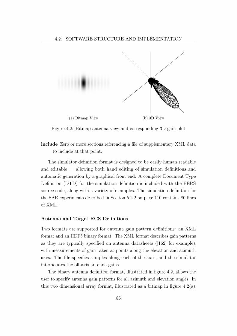
4.2. SOFTWARE STRUCTURE AND IMPLEMENTATION
(a) Bitmap View (b) 3D View
Figure 4.2: Bitmap antenna view and corresponding 3D gain plot
include Zero or more sections referencing a file of supplementary XML data
to include at that point.
The simulator definition format is designed to be easily human readable
and editable — allowing both hand editing of simulation definitions and
automatic generation by a graphical front end. A complete Document Type
Definition (DTD) for the simulation definition is included with the FERS
source code, along with a variety of examples. The simulation definition for
the SAR experiments described in Section 5.2.2 on page 110 contains 80 lines
of XML.
Antenna and Target RCS Definitions
Two formats are supported for antenna gain pattern definitions: an XML
format and an HDF5 binary format. The XML format describes gain patterns
as they are typically specified on antenna datasheets ([162] for example),
with measurements of gain taken at points along the elevation and azimuth
axes. The file specifies samples along each of the axes, and the simulator
interpolates the off-axis antenna gains.
The binary antenna definition format, illustrated in figure 4.2, allows the
user to specify antenna gain patterns for all azimuth and elevation angles. In
this two dimensional array format, illustrated as a bitmap in figure 4.2(a),
86

4.2. SOFTWARE STRUCTURE AND IMPLEMENTATION
Figure 4.3: Bistatic RCS (in dBm2) of an F5 fighter for transmitter at (-60,60) (data courtesy of Professor Keith Palmer, University of Stellenbosch)
samples of the antenna gain are specified on a rectangular grid in azimuth
and elevation. The grid spans π radians in elevation and 2π radians in
azimuth. The grid spacing is user defined, and gains between the grid points
are calculated by the simulator using cubic spline interpolation [62]. Figure
4.2(b) shows a 3D view of the antenna gain pattern corresponding to the
bitmap in figure 4.2(a).
Monostatic target RCS patterns are specified in the same way as antenna
gain patterns, using either the XML or binary format. Bistatic RCS patterns
are a function of four variables (arrival azimuth and elevation, and departure
azimuth and elevation), and are stored in an HDF5 file as a four dimensional
binary array.
Figure 4.3 illustrates the bistatic RCS of an F5 fighter for a transmitter
at 60 azimuth and −60 elevation, with the fighter pointing down the y axis
and the colour scale in dBm2. This is a three dimensional representation of a
single two-dimensional slice of the entire bistatic RCS function.
87

4.2. SOFTWARE STRUCTURE AND IMPLEMENTATION
Signal Definition
Signal definitions are stored as 64bit floating point samples in an HDF5 binary
file. The signal is stored as samples of the complex envelope (see Section 2.1.3
on page 15) of the transmitted signal. The real (inphase) and imaginary
(quadrature) parts of the signal are stored in separate columns.
4.2.2 Implementation of World Model
The world model calculates the parameters of each response (transmitter-
receiver pair or receiver-target-transmitter triple), building work lists which
the renderer uses to create the simulated data. The world model interfaces
with the renderer through a set of work stacks, one per receiver, and is allowed
to run to completion before the renderer starts.
The world model is completely multithreaded, allowing the simulator to
take advantage of SMP systems and multicore CPUs.
Algorithm 2 World model flow
Load XML file with environment description
Build lists of transmitters, receivers and targets
Add transmitters and receivers for simulated multipath
for i = 1 to the number of receivers do
while Running threads is equal to limit do
Wait
end while
Create work stack for receiver i
Create thread for receiver i
Call world model in thread
end for
88

4.2. SOFTWARE STRUCTURE AND IMPLEMENTATION
Algorithm 3 World model controller flow
for j = 1 to number of transmitted pulses do
Add direct propagation from transmitter j to receiver i to work stack
for k = 1 to number of targets do
Add propagation from transmitter j via target k to receiver i to work
stack
end for
end for
Pass work stack to environment model
Algorithm 4 Environment model flow
for i = 1 to the number of items in work stack do
if Item i is a direct propagation then
Calculate receive and transmit antenna gain in relevant direction
Calculate propagation loss
Calculate range (R) and dRdt
else
Calculate receive and transmit antenna gain in direction of the target
Calculate propagation losses
Calculate receive range (Rr) and transmitter range (Rt) to the target
Calculate dRr
dtand dRt
dt
Calculate target RCS
end if
Calculate polarization effects
end for
4.2.3 Work Stack Entries
Each work stack entry corresponds to a single transmitted pulse (or entire
waveform, for CW systems), from a single transmitter, received by a single
receiver, and optionally via a single target. Work stack entries differ between
long pulses and short pulses. For short pulses, the world model assumes that
the first derivatives of range and power are constant (note that this is not
89

4.2. SOFTWARE STRUCTURE AND IMPLEMENTATION
equivalent to the stop-go assumption used in some other radar simulators,
which assumes these derivatives are zero). For longer pulses and CW, the
work stack entry consists of a number of samples of these parameters, which
are interpolated to calculate the values of these parameters in the renderer.
The number of samples taken during the pulse interval is set in the simulation
definition.
Each interpolation point contains the power, range, phase shift and Doppler
shift for the pulse at the time of that interpolation point. Short pulse work
list items contain two interpolation points — one at the beginning of the
pulse and one at the end. Long pulse work list items contain a number of
interpolation points set by the user. In addition to interpolation points, work
list items contain the transmitted waveform, and the transmitter parameters
including power and noise temperature.
4.2.4 Implementation of Renderer
The renderer consists of three sections, the thread controller, the response
renderer and the window renderer. The thread controller section is run once
per receive window, and calls the response renderer, as required, per response.
The window renderer combines the responses to form the signal as seen in
the receiver’s receive window.
The renderer is completely multithreaded, allowing the simulator to take
advantage of SMP and multicore computers.
Thread Controller
The thread controller takes a worklist for the pulses seen by the receiver from
the world model, and calls the other renderer sections to render each receive
window. It is run once per receive window. The flow of the thread controller
is:
The thread controller ensures that the optimum number of threads are
running until the worklist is complete. The simulator implementation assumes
this number is equal to the number of cores in the machine. As the thread
controller is not computationally intensive and spends the majority of the
90

4.2. SOFTWARE STRUCTURE AND IMPLEMENTATION
Algorithm 5 Thread controller flow
Launch window renderer threadfor i = 1 to limit of render threads per window do
while Number of render threads is equal to global limit doWait
end whileLaunch response renderer thread
end for
time waiting, it is not included in the total thread count.
Response Renderer
The response renderer modifies the transmitted signal to produce the response
received by the receiver for each transmitter-target pair. In the notation
developed in Section 2.1.1 on page 13, the response renderer calculates
yijk[n] = Ri (Eijk (Tj (x[n]))) . (4.1)
The flow of the response renderer is:
Algorithm 6 Response renderer flow
while Work list not empty doLock work list mutexPop work unit x from work listUnlock work list mutexfor i = 1 to the number of samples in x[n] do
Calculate the phase shift, time shift and amplitude at the time of ix[i] = x[i] * amplitudeDesign fractional delay filter for the time shift (see Section 4.3)Apply filter to x[i]x[i] = x[i] * amplitude * exp (−j ∗ phase shift)
end forAdd results to local window
end whileLock render window mutexAdd local window to receive windowUnlock render window mutex
91
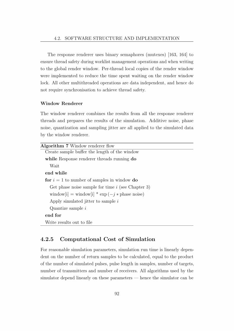
4.2. SOFTWARE STRUCTURE AND IMPLEMENTATION
The response renderer uses binary semaphores (mutexes) [163, 164] to
ensure thread safety during worklist management operations and when writing
to the global render window. Per-thread local copies of the render window
were implemented to reduce the time spent waiting on the render window
lock. All other multithreaded operations are data independent, and hence do
not require synchronisation to achieve thread safety.
Window Renderer
The window renderer combines the results from all the response renderer
threads and prepares the results of the simulation. Additive noise, phase
noise, quantization and sampling jitter are all applied to the simulated data
by the window renderer.
Algorithm 7 Window renderer flow
Create sample buffer the length of the window
while Response renderer threads running do
Wait
end while
for i = 1 to number of samples in window do
Get phase noise sample for time i (see Chapter 3)
window[i] = window[i] * exp (−j ∗ phase noise)
Apply simulated jitter to sample i
Quantize sample i
end for
Write results out to file
4.2.5 Computational Cost of Simulation
For reasonable simulation parameters, simulation run time is linearly depen-
dent on the number of return samples to be calculated, equal to the product
of the number of simulated pulses, pulse length in samples, number of targets,
number of transmitters and number of receivers. All algorithms used by the
simulator depend linearly on these parameters — hence the simulator can be
92
4.2. SOFTWARE STRUCTURE AND IMPLEMENTATION
02
46
8
0
1
2
3
40
1
2
3
4
5
6x 10
6
Log10
of
pulse length
Log10
of
number of targets
Ret
urn
Sam
ples
Per
Sec
ond
Figure 4.4: Simulator performance in return samples per second versustransmitted pulse length and target count
said to run in O(N) time, where
N =NxNtargNtransNrecvt
PRI(4.2)
and Nx is the pulse length, t is the simulation interval and PRI is the system
pulse repetition interval. For CW simulations, tPRI
= 1.
Figure 4.4 presents simulator performance versus pulse length and target
count. Simulator performance increases for large numbers, as startup over-
heads such as loading the script and pulse data dominate simulation time
for small N . Performance reaches a plateau for large numbers of targets and
pulse lengths, demonstrating the O(N) nature of the simulation algorithm.
The performance in figure 4.4 was achieved on a modestly priced quad
core PC, with four cores at 2.4GHz (Intel Core 2 Quad Q6600) and 2GB of
RAM. In this example, peak performance achieved was 5.63× 10⁶ samples
per second. This performance corresponds to realtime simulation of an air
search radar with a PRF of 400Hz, pulse width of 10µs, bandwidth of 25MHz
and 50 targets, or a CW simulation with bandwidth of 5.6MHz requiring
93

4.2. SOFTWARE STRUCTURE AND IMPLEMENTATION
100
102
104
106
10810
4
105
106
107
Pulse Length (Samples)
Ret
urn
Sam
ples
Per
Sec
ond
Four CPUsSingle CPU
Figure 4.5: Simulator performance in return samples per second versustransmitted pulse length
approximately one second of runtime per second of simulated time per target.
A small decrease (approximately 5%) in performance is visible for large
pulse lengths. Measurement with the Callgrind [143] cache and memory
simulation tool based on the Valgrind [165, 166] binary instrumentation
framework indicates that this is due to an increase in L2 data cache misses
[167] with increasing working set size. The most significant cause of L2 data
cache misses in the simulator is rendering data replacing the work stack entries
in the data cache, causing cache misses when these entries are accessed.
SMP Scaling
Due to the multithreaded nature of the world model and signal renderer,
simulator performance scales well with increasing processor count on sym-
metric multiprocessing (SMP) computers. Figure 4.5 compares simulator
performance between a single CPU and four CPUs on the same hardware.
The simulator is marginally faster on a single CPU for very small simula-
tions (N 100) due to reduced thread management overhead, but performs
significantly better on multiple processors for larger simulations. Figure 4.6
illustrates the improvement factor achieved by running the simulator on a
94

4.2. SOFTWARE STRUCTURE AND IMPLEMENTATION
100
101
102
103
104
105
1060.5
1
1.5
2
2.5
3
Pulse Length (Samples)
SM
P S
peed
up
Figure 4.6: Simulation time reduction versus pulse length for a four core SMPcomputer
four core SMP computer. Significant performance improvements are visible
for N > 100, converging on an improvement of approximately three times.
The Karp-Flatt metric [168] is widely used to estimate how well a com-
putation task parallelizes. In the model used by the Karp-Flatt metric,
parallelization seeks to reduce the serial portion e, defined as:
e =1ψ− 1
p
1− 1p
, (4.3)
where ψ is the speedup observed when the program is run on p processors.
The speedup ψ is defined as the ratio:
ψ =T1
Tp, (4.4)
where T1 and Tp are the runtime of the program when run on 1 processor and
p processors, respectively. Using this metric, and the data from figure 4.5,
the serial portion e for large N can be estimated at ≈ 11%.
95

4.2. SOFTWARE STRUCTURE AND IMPLEMENTATION
4.2.6 Extending Parallelization to Cluster Computers
MapReduce [169] is a pattern for the parallelization of programs based on a
generalization of the map and reduce higher-order functions from functional
programming ([170] or [171], for example). The MapReduce pattern allows
simple parallelization of computing tasks on many types of computers, in-
cluding clusters [169, 172], shared memory symmetric multiprocessing (SMP)
computers [173] and heterogeneous multicore computers [174]. The term
MapReduce is used in this section to apply to the pattern only, and not the
implementation of the same name from Google, Inc.
The higher-order function map applies a function to a list of elements.
Given the list a = [b, c, d] and the function f(x), the function map f a will
return [f(b), f(c), f(d)]. The higher-order reduce (or fold) function combines
a list of elements to produce a single value. Given the list a = [b, c, d] and
the function f(x, y), the function reduce f a will return f(a, f(c, d)), using
the ’right fold’ and f(f(a, b), c) using the ’left fold’.
The MapReduce model breaks a computation task up into two subtasks:
a map task and a reduce task. The map tasks performs the map higher
order function on a list of key/value pairs to produce an intermediate list of
key/value pairs. The reduce task performs the corresponding higher order
function on the intermediate list, to merge all the intermediate list items with
the same key. Examples of this process for a variety of computation tasks are
provided by Dean and Ghemawat [169].
FERS as a MapReduce Problem
The FERS renderer can be expressed as two MapReduce problems. The
input to the first process would be a list of the signals transmitted from each
transmitter in the environment. The first map step would produce a list of
scattered signals for each transmitter/scatterer pair, which would be reduced
to a list of scattered signals from each scatterer by the first reduce step. This
process would be equivalent to the calculation of the results of Eijk for all
j and k in equation 4.1. The second MapReduce problem would then map
the list of scatterer/scattered signal pairs onto a list of scattered signals for
96
4.3. FRACTIONAL DELAY FILTER DESIGN
each scatterer/receiver pair. The final reduce function would sum this list to
produce a list of received signals for each receiver, completing the evaluation
of equation 4.1.
The operations performed by such an implementation would be the same
as those performed by the renderer implementation described in Section 4.2.4.
The two implementations are therefore equivalent, and the FERS renderer can
be considered an application specific implementation of the MapReduce model.
While the current implementation scales efficiently on SMP machines, its
equivalence to a MapReduce problem suggests that it could be implemented
to scale efficiently on large computing clusters.
4.3 Fractional Delay Filter Design
In order to relax the stop-go limitation — the assumption that the round
trip time is constant during a pulse — the simulator must be able to apply a
time-varying group delay to each sample of the simulated pulse. Typically,
this group delay will not be an exact multiple of the sample time, and a
fractional sample delay is required. FIR fractional delay filters are well suited
to this application, as they are computationally efficient and offer acceptable
performance.
This section discusses the derivation and implementation of a design
process for FIR fractional delay filters which offers sufficient computational
efficiency to be executed per-sample.
4.3.1 Ideal Fractional Delay Filters
In a continuous time system, an ideal delay applied to the signal x(t) can be
expressed as:
y(t) = x(t− d), (4.5)
where d is the delay in seconds. In a discrete time system, this becomes:
y[n] = x[n− df0], (4.6)
97

4.3. FRACTIONAL DELAY FILTER DESIGN
where f0 is the system sample rate. Taking the z transform of the system
expressed by equation 4.6 yields
H(z) = z−df0 , (4.7)
which corresponds to a digital allpass filter with the transfer function
H(ejω) = e−jωd. (4.8)
Equation 4.7 can be implemented directly as a finite length FIR filter where
df0 ∈ Z. Where the delay is not an integer number of samples, this transfer
function must be realized using the family of filters known as fractional delay
filters (FD filters) [175, 176].
The ideal FIR implementation of fractional delay filters is most simply
derived from the Shannon interpolation formula [30, 28]:
x(t) =∞∑
n=−∞x[n] sinc (tfs − n) . (4.9)
The samples of the fractionally delayed signal x(t − d), can therefore be
represented as:
x(t− d) =∞∑
n=−∞x[n] sinc
((t− d)fs − n
). (4.10)
The samples of the fractionally delayed signal y[k] (equation 4.6) can therefore
be expressed as:
y[k] =∞∑
n=−∞x[n] sinc
(k + dfs − n
), (4.11)
which is equivalent to convolution of x[n] with an infinite length FIR lowpass
filter with a transition frequency of fs/2.
Direct implementation of a fractional delay such a FIR filter is not desirable,
as it requires O(N2) processing time for x[n] with length N . Truncation of
this infinite length filter is therefore required.
98

4.3. FRACTIONAL DELAY FILTER DESIGN
4.3.2 Window Design of FIR FD Filters
Window design of FIR filters [29, 177] is simple, robust, computationally
efficient, guaranteed to converge, and approaches the performance of the
best known FIR filter design methods available for FD filters [178, 179]. The
choice of window and window parameters is critical in realising optimum
performance from fractional delay filters. The Hamming [180], von Hann
[179], and Kaiser [181, 182, 183] windows have been applied to the design of
FD filters.
The window design of FIR filters is performed by truncating the number
of filter coefficients and applying a suitable window function to the remaining
coefficients. The choice of window function influences the transition width,
passband ripple and stopband attenuation [29, 134] of the resulting filter.
The Kaiser (or I0-sinh) window [184, 185] is an approximation, using the
modified Bessel function of order zero of the first kind [186], of the prolate
spheroidal wave functions [187] which provide a least-squares optimal tradeoff
between the time and frequency domain widths of the window function [134]
and hence maximize the ratio between mainlobe and sidelobe energy. The
Kaiser window function is defined as
w(k) =
I0
(β√
1−(k/N)2)
I0(β), |k| ≤ N
0, |k| > N
(4.12)
where I0(x) is the modified Bessel function of the first kind [61], N is the
width of the window in samples, and β is the window shape parameter.
Effects of N and β
The Kaiser window parameters β and N make this window good for the
implementation of an adjustable FIR fractional delay filter design procedure,
as the requirements for filter size (and hence computational cost), passband
ripple, and bandwidth can be adjusted for the application in question.
In fractional delay filter design, the window shape parameter β represents
a tradeoff between ripple in the passband and limited bandwidth. Figure
99

4.3. FRACTIONAL DELAY FILTER DESIGN
0
5
100 1 2 3 4 5 6
0.6
0.7
0.8
0.9
1
1.1
1.2
Frequency
Kaiser β
Mag
nitu
de
(a) System frequency response versus β for N = 32
0 0.1 0.2 0.3 0.4 0.5 0.6 0.7 0.8 0.9 1−3
−2.5
−2
−1.5
−1
−0.5
0
0.5
1
Normalized Frequency
Fre
quen
cy R
espo
nse
(dB
)
β = 0.1β = 5β = 10
(b) Cuts through β = 0.1, β = 5 and β = 10
Figure 4.7: The effect of Kaiser window β parameter on the frequency responseof a FIR fractional delay filter with N = 32
100

4.3. FRACTIONAL DELAY FILTER DESIGN
0.8 0.85 0.9 0.95 1−3
−2.5
−2
−1.5
−1
−0.5
0
0.5
Normalized Frequency
Fre
quen
cy R
espo
nse
(dB
)
32 Samples64 Samples128 Samples
Figure 4.8: The effect of filter length on the frequency response of a FIRfractional delay filter (β = 5)
4.7 illustrates the effects of β on the frequency response of a fractional delay
filter with N = 32 and d = 0.5/fs. For small β, the filter is within 2dB of
the ideal flat response up to 0.49fs, at the cost of 1.4dB peak-to-peak ripple
in the passband. For larger β, the ripple is reduced, but the system passband
is significantly narrowed. The ideal allpass response is flat across the entire
frequency range.
The Kaiser window has the same mainlobe width as the Hamming window
for β = 5.441, and the Blackman window for β = 8.885 [134]. The Kaiser
window offers reduced ripple and better stopband attenuation than these
windows for the same mainlobe width.
The length of the truncated filter represents a tradeoff between the system
passband and the computational cost of filter implementation. Figure 4.8
illustrates the effects of the filter length N on a Kaiser windowed fractional
delay filter with β = 5 and d = 0.5/fs. The figure clearly shows that the
system passband tends towards the ideal allpass response as for increasing N .
Each doubling of N approximately halves the width of the transition band.
For the simulation of radar systems where the pulses are oversampled,
101

4.3. FRACTIONAL DELAY FILTER DESIGN
even by a small amount, the ideal tradeoff is a large β, for example 5 ≤ β ≤ 10
and a short filter (e.g. N = 32 is sufficient in the case where the waveform is
oversampled by 10%). Where the radar waveform is close to critically sampled
the tradeoff is between significantly larger N (and hence longer computation
times) and passband ripple due to decreased β.
The window design of FIR fractional delay filters is efficient, simple and
offers excellent performance for oversampled signals. Alternative direct FIR
filter design procedures are likely to be too computationally expensive for
execution on a per-sample basis. While the Farrow [188] structure provides
another alternative to the direct implementation of fractional delays which is
well suited to time-varying delay applications, the associated computational
costs are higher than for the table-based implementation of windowed FIR
FD filters.
4.3.3 Implementation
The subsample filter design and application process requires O(NM) runtime
for window length N and signal length M . As the window length is constant,
and small compared to the signal length, it can be assumed that the process
runs in linear time. The most computationally expensive part of the imple-
mentation of the filter design process is the computing of the modified Bessel
function I0(x) used by the Kaiser window. The modified Bessel function of
the first kind is defined as [61]:
Iv(x) = (1
2x)v
∞∑n=0
(14x2)n
n!Γ (v + n+ 1), (4.13)
which, for order zero, simplifies to [134]:
I0(x) = 1 +∞∑n=1
[(x/2)n
n!
]2
. (4.14)
The Kaiser window requires values of I0(x) in the range [0, β]. FERS uses
a twelfth order polynomial approximation to I0(x) (from Abramowitz and
Stegun [61]), with a maximum error of 8×10⁻⁸ in the range [0, 20]. Using this
102

4.3. FRACTIONAL DELAY FILTER DESIGN
0 5 10 15 20 25 30
−1
−0.5
0
0.5
1x 10⁻⁸
Sample
w(x
)−w
poly
(x)
Figure 4.9: Error of polynomial approximation of Kaiser window function (N= 32, β = 5)
polynomial approximation, the approximated Kaiser window function wpoly(x)
is defined. Figure 4.9 illustrates the error in the approximated function,
compared to the exact Kaiser window function w(x) (equation 4.12).
For moving targets, transmitters or receivers (where dRdt
is non-zero), the
delay filter is recalculated for each sample and convolved with the input
signal x[n] to produce the output signal y[k]. As an optional optimisation, the
simulator builds a table of precalculated subsample delay filters, for subsample
delays in the range [−0.5, 0.5]. The filter is extracted from this table for the
subsample delay value of each sample.
In this approach, T × M filter co-efficients are calculated at program
startup, where T is the number of entries in the table and M is the filter
length. As the filter table lookup is a cheap operation, the table based
approach reduces runtimes for T ×M N , for N defined in equation 4.2
on page 93. The processing speed gain due to this approach depends on the
simulation parameters, and will be largest when Nx is the dominant factor in
equation 4.2. Callgrind [143] measurements show that this approach decreases
runtime by approximately 30% for the SAR simulations described in Section
5.2.2.
103

4.4. CONCLUSION
−0.5 −0.4 −0.3 −0.2 −0.1 0 0.1 0.2 0.3 0.4 0.5−120
−110
−100
−90
−80
−70
−60
−50
−40
Distance from entry (entries)
Pea
k E
rror
(dB
)
100 Entries1000 Entries10000 Entries
Figure 4.10: Peak subsample delay error versus distance from filter tableentry
The loss in accuracy due to the table based approach depends on the level
of quantization of the fractional delay, and hence on the number of table
entries T . Figure 4.10 illustrates the peak error caused by using filters from
the lookup table versus offset from the table entries (d× T − bd× T + 0.5c,where d is the subsample delay). For a table of 10000 entries, requiring
approximately 2.6MB of memory, the peak error is approximately −83dB.
For comparison, the peak error for an implementation without subsample
accuracy is approximately −6dB.
Sample accurate group delay implementation simulates the Doppler effect
on baseband signals, and complex envelope of bandpass signals. Validation
of the performance of the baseband Doppler implementation using bistatic
sonar measurements is presented in Section 5.3.2 on page 119.
4.4 Conclusion
The FERS simulator, as described in this chapter, consists of approximately
9000 lines of C++ code implementing the simulation model described in
Chapter 2 and the synthetic phase noise generation algorithm described in
104

4.4. CONCLUSION
Chapter 3. In addition, the simulator includes over 1500 lines of support
code in MATLAB, Python and C++. The complete source code for the FERS
simulator is freely available under the GNU GPL [152] version 2.
As described in section 4.2, the simulator implementation is divided into
two parts: the world model and the signal renderer. The world model produces
a high level description of the simulator output in XML format and provides
these results to the signal renderer. The renderer combines the world model
results to produce complete raw signal results for all simulated receivers. The
complete simulator supports arbitrary radar configurations, including numbers
of transmitters, receivers and targets limited only by available memory.
FERS runs well on modern PC hardware, with typical simulations (see
Section 4.2.5 on page 92) taking from a few seconds to several minutes.
Modern SMP PC hardware, including mass market multicore hardware, offers
a nearly linear speed up with processor count for large simulation tasks.
105
Chapter 5
Validation of Simulator
Accuracy
5.1 Introduction
Validation of the accuracy of the simulation model and implementation
was performed using two approaches: comparison of simulation results with
theoretical expectations, and comparison of simulations with measurements
from the NetRad [76, 77, 78] netted radar and a bistatic sonar system. This
chapter presents the results of these comparisons, and discusses the conclusions
which can be drawn about the accuracy of the simulation results from each
step of the validation process.
The validation programme was specifically designed to validate two types
of simulator behaviour: the accuracy of simulation of phenomena explicitly
implemented in the model, and the accuracy of emergent behaviours which
are not explicitly implemented. Emergent behaviours reflect the ability of
the simulator to predict aspects of radar performance beyond the scope of
the simulation model. Validation of these behaviours tests many aspects of
simulator performance.
The comparisons described in this chapter show that simulation results
match measured results with a high degree of accuracy, and suggest that
simulation results for other systems will be accurate.
106

5.2. COMPARISON WITH THEORETICAL PREDICTIONS
5.2 Comparison with Theoretical Predictions
Radar signal processing techniques, such as moving target indication (MTI)
and synthetic aperture radar (SAR) use the phase and amplitude of the
received pulse to reject clutter (in MTI) and improve cross-range resolution
(in SAR). These techniques are based on theoretical predictions about the
properties of the received information. Processing simulated radar signals
using these techniques will measure how accurately the simulated results
match the predictions that the processing is based on, and hence will measure
the accuracy of some aspects of the simulation results.
5.2.1 Moving Target Identification Radar
The term moving target identification (MTI) is typically applied to radars
operating at a low PRF which enhance the detection of moving targets through
application of time-delay cancelers. The simplest such canceller, the two pulse
canceller, outputs the vector difference between two consecutive pulses [145]:
xo[t+ PRI] = xi[t]− xi[t+ PRI], (5.1)
where PRI is the system pulse repetition interval. For a single target return
processed by a two pulse canceller, the output power is 4 sin2(πfdPRI), where
fd is the Doppler frequency of the target. When the target Doppler frequency
is a multiple of the system PRF the target will be cancelled along with the
clutter — these frequencies are referred to as blind frequencies.
Improved cancelers and processing techniques are available which seek
to sharpen the notch at zero Doppler (cascaded delay cancelers) and reduce
blind frequencies (PRF stagger). While these systems will not be considered
in this section, the conclusions presented here also apply to these types of
processing.
A key performance attribute for MTI systems is the improvement factor
[144] — “The signal-to-clutter ratio at the output of the clutter filter divided
by the signal-to-clutter ratio at the input of the clutter filter, averaged
uniformly over all target radial velocities of interest” [189]. Errors in the
107

5.2. COMPARISON WITH THEORETICAL PREDICTIONS
receiver LO frequency limit the improvement factor to [144, 145]:
IdB = 20 log10
(1
2πδfT
), (5.2)
where T is the round trip propagation delay, and δf is the pulse to pulse
frequency change.
Figure 5.1 compares the results of simulation of the effects of receiver LO
frequency drift on MTI improvement factor with the theoretical limit. The
simulation was structured to ensure that LO frequency drift was the limiting
factor on MTI improvement. The simulated and theoretical results agree very
closely at both short (20km) and long (210km) ranges.
Another limit on the MTI improvement factor is antenna scan modulation:
the return power changes between views caused by the antenna gain pattern.
The clutter power standard deviation due to scanning with a Gaussian pattern
antenna is [144]:
σc = 0.265SrWb, (5.3)
where Sr is the antenna scan rate (in degrees per second) and Wb is the −3dB
beamwidth of the antenna, in degrees. The improvement factor limit for a
three delay canceller is [50]:
z =2πσcPRF
(5.4)
I2 =(1− 4
3exp
(−z2
2
)+
1
3exp
(−2z2
))−1. (5.5)
Figure 5.2 compares the results of simulation of the improvement factor of
an MTI system versus the limit from equation 5.5. The simulated system has
an antenna beamwidth of 6, scan rate of 360 per second and other parameters
chosen to ensure that the improvement factor is limited by scan modulation.
The simulated results and theoretical predictions match extremely closely
over the entire range of pulse repetition frequencies simulated.
Comparison of the results of the simulation of an MTI system with
theoretical performance predictions revealed very close agreement between
theory and predictions. The phenomena tested by the simulation of MTI
108

5.2. COMPARISON WITH THEORETICAL PREDICTIONS
0 20 40 60 80 100 1200
5
10
15
20
25
30
35
40
45
Receiver LO Frequency Offset (Hz)
MT
I Im
prov
emen
t Fac
tor
(dB
)
Theoretical LimitSimulation Results
(a) 420km Round Trip
0 200 400 600 800 1000 12000
10
20
30
40
50
60
70
Receiver LO Frequency Offset (Hz)
MT
I Im
prov
emen
t Fac
tor
(dB
)
Theoretical LimitSimulation Results
(b) 40km Round Trip
Figure 5.1: Comparison simulated MTI improvement versus theoreticallypredicted limit
109

5.2. COMPARISON WITH THEORETICAL PREDICTIONS
1 2 3 4 5 6 7 8 9 1020
30
40
50
60
70
80
90
PRF (kHz)
MT
I Im
prov
emen
t Fac
tor
(dB
)
Simulated PerformanceTheoretical Prediction
Figure 5.2: MTI Improvement factor limitation due to antenna scan modula-tion
systems are not explicitly implemented in the simulation model, and are
emergent behaviours of the model.
5.2.2 Synthetic Aperture Radar
Synthetic aperture radar (SAR) is a type of radar signal processing which
simulates the effect of a narrow beam (or long aperture) by performing signal
processing on a train of received pulses [190, 191]. Conceptually, the simplest
type of SAR is airborne stripmap SAR, where an aircraft is flown along a
linear track with an antenna looking sideways at a swath of ground. Figure
5.3 illustrates the geometry of an ideal stripmap SAR system.
The South African SAR system (SASAR) is a VHF SAR sensor [192, 193]
designed and built in South Africa during the 1990s. Part of the project was
the development of an advanced Range-Doppler SAR processing suite, titled
G2 [10, 194]. This section presents the results of simulation of a SAR system
with the same parameters as SASAR, with the results processed with the G2
SAR processor. Table 5.1 lists the parameters of the SASAR system used in
the simulations in this section.
110

5.2. COMPARISON WITH THEORETICAL PREDICTIONS
(a) Side view (after [10]) (b) Top view
Figure 5.3: Airborne Stripmap SAR Geometry
Table 5.1: SASAR System Parameters (after [10])
Parameter ValueCentre Frequency 141MHzBandwidth 12MHzPulse modulation monochromaticPRF 545HzGround Speed 90 ms−1
Altitude 4000 mAzimuth Beamwidth 60
Elevation Beamwidth 60
Sample rate 24MHz
111

5.2. COMPARISON WITH THEORETICAL PREDICTIONS
(a) SAR Image
−150 −100 −50 0 50 100 150
−30
−25
−20
−15
−10
−5
0
Along Track Range (m)P
ower
(dB
)
(b) Cut through target
Figure 5.4: Processed results of VHF SAR simulation with single target
Figure 5.4 illustrates a SAR image of a single target, simulated with FERS
and processed with G2. The image in 5.4(b) spans 1245m in slant range by
165m in along track range. Four seconds of simulated data were generated,
corresponding to a synthetic aperture of 360m. The image clearly shows a
single, sharpened target — demonstrating that the phase calculations in the
simulator match the theoretical predictions used by focused SAR processing.
Figure 5.5 is a multiple target test, with the targets spaced 80m apart in along
track range and 200m apart in ground range. This test case demonstrates
that phase calculations are valid at all ranges.
Increasing the effective synthetic aperture of a SAR system improves
resolution, and reduces the width of a single target. Figure 5.6 illustrates the
effects of increasing the synthetic aperture on the sharpness of a single target.
Results are presented for 1s, 2s and 10s of data.
Deviations in the trajectory of the radar sensor reduce the accuracy of
SAR processing, as the phases of consecutive pulses can no longer be precisely
aligned. Most SAR systems perform motion compensation using measure-
ments of the platform’s position to correct for these deviations. The G2
processor, for example, can perform motion compensation using measure-
ments from GPS and an inertial platform [10].
Figure 5.7 on page 114 shows the effects of uncorrected sensor trajectory
112
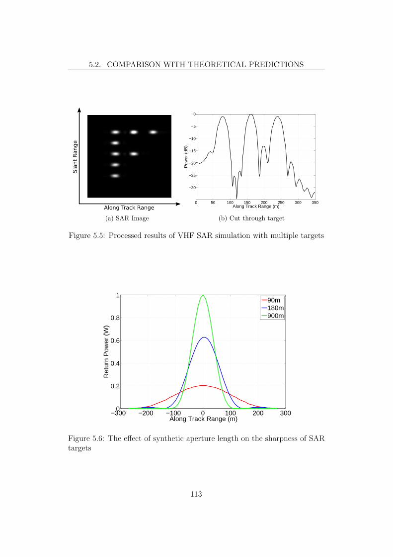
5.2. COMPARISON WITH THEORETICAL PREDICTIONS
(a) SAR Image
0 50 100 150 200 250 300 350
−30
−25
−20
−15
−10
−5
0
Along Track Range (m)
Pow
er (
dB)
(b) Cut through target
Figure 5.5: Processed results of VHF SAR simulation with multiple targets
−300 −200 −100 0 100 200 3000
0.2
0.4
0.6
0.8
1
Along Track Range (m)
Ret
urn
Pow
er (
W)
90m180m900m
Figure 5.6: The effect of synthetic aperture length on the sharpness of SARtargets
113

5.2. COMPARISON WITH THEORETICAL PREDICTIONS
0 50 100 150 200 250 300 350
−35
−30
−25
−20
−15
−10
−5
0
Along Track Range (m)
Pow
er (
dB)
Perfect TrajectoryUncorrected Trajectory Deviations
Figure 5.7: Effect of sensor trajectory deviations on SAR processing
deviations as a cut through the target. In this example, the altitude was
perturbed with a sinusoidal modulation with an amplitude of 0.25m and a
period of 2s. The results clearly illustrate how sensor trajectory deviations
reduce the integrated sidelobe ratio (ISLR) and increase the peak sidelobe level
— corresponding to the along track blurring of SAR images. A discussion of the
effects of local oscillator phase noise on SAR processing, and its equivalence
to uncompensated motion errors, is presented in Appendix A.
These results of from SAR processing provide a qualitative demonstration
of the accuracy of the simulation of a VHF SAR system produced by FERS.
In each case, the parameters of the processed SAR image depend on the pa-
rameters of the simulation in the way predicted by theory. This demonstrates
the accuracy of phase calculations, and the simulation of systems with moving
sensors.
5.2.3 Passive Coherent Location
A passive coherent location (PCL) radar is a multistatic radar system which
uses non-cooperating ’illuminators of opportunity’ instead of a traditional
transmitters [195]. Suitable illuminators include FM radio transmissions
[196, 197, 198, 199], analog television [200, 201], GSM cellular telephone
transmitters [202] and satellite transmitters [203]. The advantages of PCL
114

5.2. COMPARISON WITH THEORETICAL PREDICTIONS
Figure 5.8: Layout of the transmitter, receiver and target for PCL simulations
include reduced cost, improved resistance to some types of stealth technology,
improved resistance to electronic counter measures and stealthy operation.
Working examples of PCL systems include the Silent Sentry air surveillance
radar from Lockheed Martin, and the Manastash Ridge system for remote
sensing of the upper atmosphere [199].
A PCL air surveillance radar, based on FM radio transmissions, is currently
under development at UCT. The prototype system will use receivers based
at UCT and the FM transmitter at Constantiaberg to track aircraft targets
approaching Cape Town International Airport. In simulation experiments
designed and performed by Sebastiaan Heunis at UCT, FERS was used to
predict the performance of the prototype simulation system. This section
demonstrates the accuracy of FERS simulations of a CW PCL system using
some of the results from these experiments.
Simply, the PCL system receives the direct (reference) signal and scattered
signal using two separate antennae. The reference signal (which is much higher
in power than the scattered signal [195]) is phase shifted and mixed with the
scattered signal channel, to attenuate the portion of the direct signal received
in that channel. Processing is performed by correlating the reference signal,
and Doppler shifted versions of the reference signal, with the scattered signal.
Figure 5.9 shows the range-Doppler plots of the processed results for
two PCL signals with 50MHz bandwidth. In figure 5.9(a), the signal used
was a one second simulated commercial FM radio signal, with the station
115

5.2. COMPARISON WITH THEORETICAL PREDICTIONS
Doppler Shift (Hz)
Del
ay (
µs)
−100 −50 0 50 1000
10
20
30
40
50
60
−30
−25
−20
−15
−10
−5
0
(a) Simulated FM radio signal
Doppler Shift (Hz)
Del
ay (
µs)
−100 −50 0 50 1000
10
20
30
40
50
60
−30
−25
−20
−15
−10
−5
0
(b) White Gaussian Noise
Figure 5.9: Range-Doppler plots for processed PCL simulation results (simu-lation by Sebastiaan Heunis)
116

5.3. COMPARISON WITH MEASUREMENTS
transmitting a metalcore (similar to punk and heavy metal music) track.
The signal used for figure 5.9(b) was white Gaussian noise with the same
bandwidth as the simulated FM signal. In both examples, processing was
performed using a frequency domain cross-correlation method.
The comparison of figures 5.9(a) and 5.9(b) clearly demonstrates that,
while the FM signal clearly shows the target, the ’ambiguity function’ (in
the sense used by Baker, et. al. [204]) for the white Gaussian noise is
closer to optimal. In both cases, the target is shown at the correct range
(approximately 36.4µs delay) and Doppler shift (approximately −59.5Hz.
Note that the delay figure refers to the difference in arrival times of the
scattered signal and reference signal. These preliminary results show that
FERS is able to simulate a CW system, and introduce the correct Doppler
and time shifts onto the return signal. The structural similarity of the results
in figure 5.9(a) and the results obtained by Baker, et. al. [204] for FM signals
suggests that the FERS simulation and processing are producing plausible
results.
These results present the first results of an ongoing process of simulating
PCL performance. They are a strong demonstration that the FERS simulator
is able to simulate a PCL system, and can be used for the prediction of PCL
performance.
5.3 Comparison with Measurements
The ultimate goal of a simulator is to produce results matching those which
would be produced by a physical system with the same specifications as the
simulated system. Comparison of simulator outputs against measured results
is therefore an extremely important step in the verification process. This
section describes two sets of verification comparisons — one with a prototype
netted radar system and one with a simple bistatic sonar system. The goal of
the netted radar comparisons was to verify the accuracy of simulations of a
multistatic pulse Doppler radar. The goal of the comparison with the bistatic
sonar was to verify the accuracy of the baseband delay (and hence Doppler)
calculations and the group delay renderer (Section 4.3).
117

5.3. COMPARISON WITH MEASUREMENTS
Figure 5.10: Netrad geometry used for validation measurements
5.3.1 Netted Radar System
Netrad [75, 76, 205, 77, 78] is an experimental pulse-Doppler netted radar
system developed at the University College London. The system has three
nodes operating at 2.4GHz, with a maximum bandwidth of 50MHz, maximum
power of −23dBm, and antenna gain of 15dBi [162]. For the comparisons
presented here, the nodes were set up as illustrated in figure 5.10.
In the default configuration, transmissions are interleaved between the
nodes (with node 1 transmitting, then node 2, then 3) with a total PRF of
20kHz. The measurements described in this section were performed with a
1.5ms linear chirp with a bandwidth of 50MHz.
A series of measurements using the Netrad system were performed by
Doughty, et. al. at UCL in July 2007. Comparisons between data from this
measurement campaign and simulations of the measured scenarios were used
to validate the accuracy of FERS simulations of netted radar systems. A
number of scenarios were simulated, including static targets, large moving
targets (such as a van), and small moving targets (such as a walking man).
In all cases, it was found that the simulated results closely matched the
measured results, taking into account the assumptions made by the radar
simulator. While the range used for the measurements was relatively free
of clutter [77], some clutter returns were still present in the measured data
— and absent in the simulations. Some types of moving targets, including
118

5.3. COMPARISON WITH MEASUREMENTS
people and vehicles, were found to be spread out over several Doppler bins,
due to microdoppler, an effect which wasn’t included in simulations of the
netted radar system.
Figures 5.11 and 5.12 present a comparison between simulated and mea-
sured results for an experiment performed with Netrad. In this experiment,
a van was driven obliquely across the range at 9ms−1 and observed using
interleaved pulses from each transmitter in turn. Pulses were received on all
three transmitters. Range-Doppler plots for pulses transmitted by Node 1
and received by Node 3 are shown in figure 5.11. The overall structure of the
simulated and measured results are identical — with the peak in range bin
15 and Doppler bin 9. Stationary clutter is present in Doppler bin 0 in the
measured data, but is clearly separated from the moving target.
Cuts through the the target in range and Doppler are presented in figure
5.12. In Doppler (figure 5.12(a)), the peak position and rolloff of the simulated
data and measured data are similar. Noise is less effectively suppressed in the
measured data, and the maximum deviation between measured and simulated
signals is small. In the range cut (figure 5.12(b)), the differences between the
simulated and measured data are small — mostly limited to clutter returns
beyond range bin 30.
While these figures only present the results of a single simulation, they
correlate well with the results of simulations of other measurements taken
with the netted radar hardware. In all cases, it was found that the processed
range-Doppler results of the simulations closely match the measured results.
The results demonstrate both the accuracy of the simulation model for bistatic
radar (Chapter 2) and the correctness of the implementation of this model.
5.3.2 Bistatic Sonar
Validation of the baseband phase and frequency shift model, and its implemen-
tation (Section 4.2.4), was performed using a bistatic CW sonar (ultrasound)
system. The sonar system used for these tests was designed and built by the
author.
Figure 5.13 illustrates the setup of the ultrasound sonar system. A 40kHz
119

5.3. COMPARISON WITH MEASUREMENTS
Range Bin
Dop
pler
Fre
quen
cy (
Hz)
10 12 14 16 18 200
50
100
150
200
250
300
−30
−25
−20
−15
−10
−5
0
(a) Measured result
Range Bin
Dop
pler
Fre
quen
cy (
Hz)
10 12 14 16 18 200
50
100
150
200
250
300
−30
−25
−20
−15
−10
−5
0
(b) Simulated result
Figure 5.11: Measured and simulated range-Doppler images for netted radarexperiment
120

5.3. COMPARISON WITH MEASUREMENTS
0 5 10 15 20 25 30−50
−40
−30
−20
−10
0
Doppler Bin
Ret
urn
Pow
er (
dB)
Measured DataSimulated Data
(a) Cut through Doppler bin 7
0 10 20 30 40 50 60−60
−50
−40
−30
−20
−10
0
Range Bin
Ret
urn
Pow
er (
dB)
Measured DataSimulated Data
(b) Cut through range bin 15
Figure 5.12: Cuts through netted radar measurement and simulation in rangeand Doppler
121

5.3. COMPARISON WITH MEASUREMENTS
40kHz
100kHz
A/DPendulumRest Point
100mm
600mm
Murata MA40B8
(a) Top view
600mm
A/D
100KHz
(b) Side view
Figure 5.13: Experimental setup for CW sonar system
12Vp−p sinusoid was generated with a signal generator and used to drive a
Murata MA40B8S [206] piezoelectric sonar transducer. A spherical pendulum
was suspended with its rest point 600mm from the center of the sonar baseline.
The return signal captured with Murata MA40B8R transducer, amplified and
sampled at 8 bits. To reduce the effects of the analog sampling process, the
signal was sampled at a rate of 200kHz, followed by polyphase downsampling
to 100kHz with a steep rolloff. Due to the extremely limited bandwidth, and
high quality factor (Q) [83], of the transducers used the received signal was
strongly bandlimited. A sample rate of 100kHz was sufficient to capture the
received signal without aliasing.
The pendulum was suspended from a fixed point 505mm above the plane of
the sonar transducers, and raised to an angle of 37 degrees. The sonar returns
were recorded for 8 seconds. The returns were normalized then analysed
with the short time Fourier transform (STFT) [207, 29], using transforms of
4096 samples, 50% overlap, and a Hamming [134] window. A simulation was
122

5.4. SIMULATION OF PHASE NOISE EFFECTS
performed using the FERS simulator, with an extension module to simulate
pendulum motion and the results processed in the same way as the measured
signal.
Figure 5.14 compares the STFTs of results of the simulation of the sonar
system with the measured results. The results show a frequency modulation of
the return signal due to motion of the target, and an unmodulated version of
the signal received directly from the transmitter. The simulated and measured
results show identical overall structure, peak Doppler (332± 0.6Hz) and ratio
between the direct and return signals.
Using the differential equation of pendulum motion,
d2θ
dt2= −g
lsin θ, (5.6)
where g = 9.81ms−1 and l = 505mm, the maximum velocity of the pendulum
is expected to be 1.41ms−1. The maximum measured bistatic Doppler is there-
fore expected to be 332.58Hz. This closely matches the maximum Doppler in
both the measured and simulated results. While equation 5.6 was used to
define the motion in the simulator extension used, the results demonstrate
that the baseband Doppler shift algorithm (based on the fractional delay
filters described in Section 4.2.4) produces the expected results. These results
also highlight the usefulness of the simulator extension mechanism.
5.4 Simulation of Phase Noise Effects
Simulation of the effects of local oscillator phase noise on radar signals is an
important feature of the FERS simulator, and the simulation model. The
pruned multirate filterbank approach to the generation of synthetic phase
noise sequences, as described in Section 3.6, allows simulation of the effects of
phase noise in pulsed systems with little increase in simulation time. Appendix
A contains two case studies of the results of simulation of phase noise effects.
While these results were not directly considered to be part of the verification
process, they provide a demonstration that the behaviour of the phase noise
generation process is correct.
123
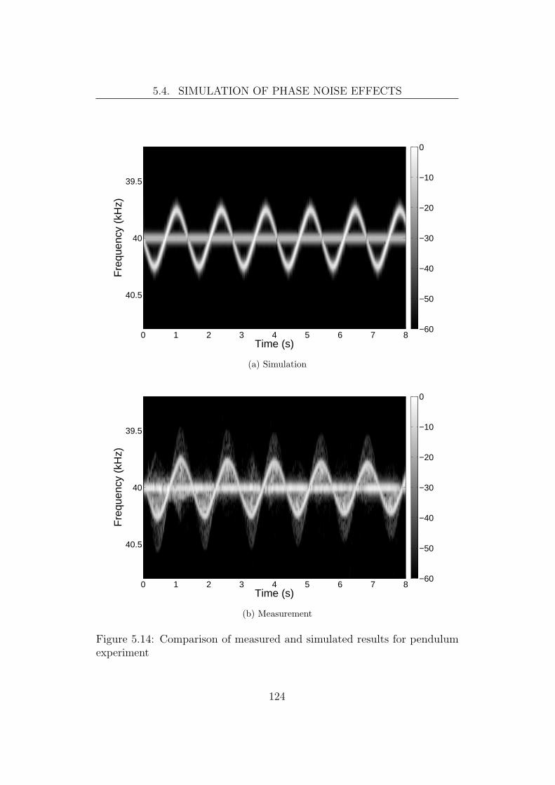
5.4. SIMULATION OF PHASE NOISE EFFECTS
Time (s)
Fre
quen
cy (
kHz)
0 1 2 3 4 5 6 7 8
39.5
40
40.5
−60
−50
−40
−30
−20
−10
0
(a) Simulation
Time (s)
Fre
quen
cy (
kHz)
0 1 2 3 4 5 6 7 8
39.5
40
40.5
−60
−50
−40
−30
−20
−10
0
(b) Measurement
Figure 5.14: Comparison of measured and simulated results for pendulumexperiment
124
5.5. CONCLUSION
The results presented in the Appendix demonstrate that the dynamic
pruning algorithm effectively preserves long range correlations in 1/f noise
processes. This can be clearly seen in the long integration time results
in the pulse-Doppler radar example (Section A.2), where the long-memory
components of phase noise cause increasing degradation of Doppler resolution.
If the long-memory nature of 1/f noise was destroyed by the generation
algorithm, the Doppler resolution would have been observed to improve over
long integration times.
5.5 Conclusion
The accuracy of the results of the FERS simulator has been demonstrated by
comparing these results to both measurements and theoretical predictions. In
the comparison to theoretical predictions, it was found that the simulations of
the behaviour of an MTI radar system closely matches the predicted behaviour
of such a system. In addition, the phase shift calculations were verified by
demonstrating that the simulated results produce a sharp SAR image, with
the targets at the expected positions. As the SAR processing was performed
with a well validated SAR processor, this strongly suggests that the simulator
results are correct to within the parameters used in SAR processing.
Comparison of simulation results to measurements taken using the NetRad
netted radar also show a high degree of correspondence. The postion of range
and Doppler peaks match between the simulated and measured results (figure
5.11), and cuts through these peaks show a nearly identical structure (figure
5.12). Further comparisons with measurements taken using a bistatic sonar
system demonstrate the correctness of the baseband Doppler shift algorithm,
and the implementation of this algorithm using FIR fractional delay filters.
The process of validating the accuracy of FERS is ongoing. Preliminary
results of work currently underway at UCT, by Yoann Paichard and Sebastiaan
Heunis, have suggested the FERS simulations of an FM radio based passive
coherent location (PCL) system match the expectations of theory. The use of
FERS in this research is likely to provide a large amount of validation data,
from both theory and measurements.
125

Chapter 6
Conclusion
6.1 Summary and Contributions
This thesis describes the design and implementation of FERS, a flexible
and extensible signal level radar simulator. FERS is capable of simulating
a diverse range of radar system designs and radar phenomena, including
arbitrary numbers of targets, transmitters and receivers. The simulator’s
extensibility and flexibility make it ideal for research and development —
supporting the student or engineer in effectively exploring the radar design
space without artificial constraints on system parameters.
FERS is also suitable for education and training. In a university envi-
ronment, the simulator could be used to demonstrate the effects of radar
parameters on output signals, to generate example signals for radar signal
processing exercises, or to provide a means for the student to test the perfor-
mance of hypothetical radar systems. Coupled with a suitable graphical user
interface (GUI) and signal processor, FERS could be used for training radar
operators and technicians.
Chapter 1 introduces the work, and describes the different philosophies
and approaches to radar systems. The diverse nature of radar is presented
to the reader, and a justification for the requirements of flexibility and
extensibility is presented. The introduction also describes the structure of
this thesis, and briefly lists the contributions of this work to the field of radar
126

6.1. SUMMARY AND CONTRIBUTIONS
simulation.
A discrete-time model for radar simulation is presented in Chapter
2. The emphasis of the model is on providing maximum flexibility while
not significantly limiting descriptive power. The structure of the model is
described, with the details of each section of the model clearly explained. The
key contributions of this chapter are:
• A radar simulation model without restrictions on the configuration of
the system under simulation. The model places no restriction on the
system geometry; the number of transmitters, receivers and targets; the
transmitted waveform; or the key parameters of the simulated system.
• The use of the superposition principle to reduce the simulation of the
return of a multistatic radar system into a linear time problem, without
placing any restrictions on the system being simulated.
Chapter 3 describes the approach used for the generation of phase
noise sequences in FERS. A model of the performance of frequency sources
tailored to radar systems, including both random and deterministic effects,
is developed. This model draws on both the radar field and the time and
frequency field, and presents the key parameters of oscillator performance in
a manner which is relevant to radar simulation. A quantitative study of a
variety of algorithms for the generation of synthetic phase noise sequences is
presented. Chapter 3 describes two contributions to the radar field:
• A multirate filterbank for the efficient generation of phase noise se-
quences matching the measured performance of high precision oscilla-
tors. While the generation of coloured noise using multirate filterbanks
has been described in the literature [7], the structure presented here
is the first which allows the power spectral density slope to change
between bands, modelling the performance of real oscillators. The use
of multirate filters for synthetic phase noise generation has not been
described in the literature in the context of radar simulation.
• A novel extension of the multirate approach to the generation of phase
noise sequences allowing the efficient generation of sparse or pulsed
127

6.1. SUMMARY AND CONTRIBUTIONS
coloured noise sequences. This approach is more efficient than any other
currently available method for generating sparse sequences of coloured
noise while preserving long term correlations.
The implementation of the simulation model as a C++ program is described
in Chapter 4. A high-level overview of the software design is presented,
and the simulator inputs and outputs described in detail. The chapter
examines the design of the two stages of simulation (the world model and
the signal renderer), and presents pseudocode for the top level flow of each
stage. Performance figures for single- and multiprocessor machines and the
design and implementation of an algorithm for the windowed design of FIR
fractional delay filters are presented. The key contributions of this chapter
are:
• The mapping of the multistatic radar simulation problem onto multi-
threaded computers by exploiting the superposition property of linear
systems.
• The use of a table of FIR fractional delay filters to efficiently and
accurately apply a subsample accurate group delay to arbitrary digital
signals. The use of this approach in a radar simulator has not been
described in the open literature, and is believed to be a novel contribution
to the field of radar simulation.
Chapter 5 presents selected results from the validation of the simulator.
Simulated results are compared against both theoretical expectations, and
measurements from a multistatic radar system. The use of the FERS for
simulating the effects of local oscillator phase noise on the performance of a
pulse-Doppler radar system is described. In addition, Appendix A describes
the use of the simulator as part of a stochastic simulation of the effects of
phase noise on Synthetic Aperture Radar.
128
6.2. FUTURE WORK
6.2 Future Work
This section describes possible future directions for research into radar simu-
lation. Areas for future work can be divided into two categories: extension of
the scope and accuracy of the simulator, and uses of the simulator to obtain
a better understanding of radar phenomena.
Radio Propagation Modelling
The free space propagation equation, as described in Section 2.2.2, does not
consider the effects of terrain and the atmosphere on the propagation of radar
signals. A more complete model, including simulation of terrain effects, would
improve the applicability of simulator results to real-world radar systems.
Research is currently underway at UCT, by Gunter Lange and others, into
combining the results of the propagation simulator AREPS [208, 209] with
the results of FERS in the context of an FM based passive coherent location
(PCL) system.
The extension of this work to the development of a simple method for
combining the results of the two simulations would increase the value of FERS
in terrain-dominated simulations. Alternatively, an open-source terrain effect
model could be implemented as an extension to FERS. In order for such a
model to be valuable, it would need to consider effects which are not included
in AREPS — such as propagation in indoor and built up environments.
The inclusion of a complete channel model in FERS would also increase
the value of the simulation in some circumstances. Such a model could
consider fading, scattering and dispersion in environments where these effects
are relevant to the performance of radar systems.
Global Illumination
The expansion of the environment model (Section 2.2) to consider multiscatter
effects (Section B.3 in Appendix B) would improve the accuracy of the
simulation algorithm in some radar applications. The most promising source
of algorithms for efficient implementation of multiscatter is likely to be the
129

6.2. FUTURE WORK
computer graphics field of global illumination (see [210] and [211] for good
introductions to the topic). Specifically, indirect illumination algorithms such
as radiosity and ray tracing are likely to prove to be adaptable to the radar
simulation problem.
Section B.3 provides a justification for the exclusion of multiscatter effects
from the simulation model described in this work. Where the assumptions
made in this section do not hold, however, the implementation of a global
illumination based simulation of multiscatter effects will increase the accuracy
of radar simulation. In addition, global illumination algorithms could provide
an extension of the limited multipath simulation model described in Section
2.2.6.
Target and Antenna Modelling
The extension of FERS to include electromagnetic simulation capabilities
would enable the simulator to calculate bistatic RCS patterns and antenna
radiation patterns dynamically, based on the requirements of the simulations.
A simple way to achieve this goal would be the development of an extension
to FERS to allow integration with an existing electromagnetic simulator (such
as FEKO [212]). The implementation of a method of moments or physical
optics code as an extension to FERS would also be desirable.
Optimisation of Radar Systems
The number of parameters which must be considered during the development
and deployment of radar systems makes direct optimisation of designs pro-
hibitively difficult, especially for netted and multistatic designs with large
numbers of sensors. Traditional engineering approaches, such as the applica-
tion of heuristics, allows workable solutions to be found — but these are not
likely to be truly optimal.
The use of a simulator such as FERS in the loop of powerful optimisation
approaches, such as genetic algorithms, could allow better optimisation of
system parameters and improve the performance-to-cost ratio of radar systems.
A future project at UCT will look at the use of a combination of FERS and
130

6.2. FUTURE WORK
AREPS for the optimisation of the placement of sensors in a PCL system.
131

Appendix A
Stochastic Simulation of Phase
Noise Effects
A.1 Introduction
This chapter presents an example of the use of FERS to investigate aspects of
radar performance which are not well covered by theory. In the case studies
presented here, FERS is used to examine the effects of phase noise on two
radar systems: a VHF SAR system, and a multistatic pulse-Doppler system.
The pulse-Doppler case study presents simulations of the effects of phase
noise on the Doppler resolution of a multistatic radar system, modelled after
NetRad [76, 205, 77, 78]. Traditional theory predicts [26] that the Doppler
resolution of such a system increases with integration time. The simulations
presented in this chapter examine the validity of that assumption in the
presence of phase noise generated by long-memory processes.
In the SAR case study, the effects of phase noise on Synthetic Aperture
Radar (SAR) processing are investigated, with the goal of deriving relation-
ships between the properties of the phase noise and SAR performance. As
in Section 5.2.2, the SASAR VHF system has been used as a model for the
simulation parameters.
In this chapter, the stochastic simulation (Monte Carlo) approach is used
to analyse the performance of radar systems in the presence of phase noise.
132

A.2. BISTATIC PULSE-DOPPLER RADAR
This approach is necessary due to the random nature of phase noise — each
run will produce different results, but general rules about performance can be
extracted from the results of multiple runs. A similar approach, with different
details, was used to analyse the performance of SAR systems in the presence
of Gaussian phase deviations by Greene and Moller [213].
The goal of this chapter is to illustrate the type of simulation and analysis
which can be performed with FERS, that can not be performed with other
widely available radar simulators.
A.2 Bistatic Pulse-Doppler Radar
As illustrated in figure 3.1 on page 43 the detectability of targets in a pulse-
Doppler radar system can be compromised by Doppler spreading of stronger
targets in the same range bin. This spreading is typically caused by local
oscillator phase noise. This effect is especially important in multistatic radar
systems, as the direct signal from a transmitter to a receiver is likely to be
much higher in power than any target responses, and is not rejected by a T-R
switch as in traditional monostatic systems.
In an ideal system, the visibility of targets separated in range and Doppler
from these high power direct signals is limited only by the ambiguity function
of the transmitted waveform. Phase noise on the receiver’s local oscillator,
however, will spread these signals out over more Doppler bins than predicted
by the ambiguity function, effectively reducing the visibility of targets close
to the direct path in range and Doppler.
In this case study, FERS was used to simulate the effects of phase noise on
a multistatic radar system similar to NetRad. The transmitter was assumed to
contain an ideal local oscillator and the phase noise on the receiver’s oscillator
was chosen to match the measured phase noise on the NetRad system. Figure
A.1 shows the phase noise curve used for simulations, based on the phase
noise measured between two nodes in the NetRad system.1
The simulator was configured with two nodes: a receiver, and a single
1Thanks to Stephan Sandenbergh at the University of Cape Town for performing thesemeasurements and sharing the results
133

A.2. BISTATIC PULSE-DOPPLER RADAR
102
104
106−120
−110
−100
−90
−80
−70
−60
Frequency (Hz)
Pha
se N
oise
(dB
c/H
z)
Specificied Phase NoisePolynomial Fit
Figure A.1: Measured phase noise of NetRad cable-based clock transfersystem, and polynomial fit
transmitter 55m away in the main beam of the receiver. No targets or
multipath effects were included in the simulation. The results from each
range-Doppler bin were taken as the mean of the return powers over 50
simulations.
A.2.1 Simulation Results
Figure A.2 illustrates the direct signal from transmitter to receiver in range-
Doppler space, with the Doppler scale in Hertz. The intensity and contours
represent power normalized to 0dB, with contours at 10dB intervals. In
the ideal case, with zero phase noise, each of these plots would be a single
horizontal line, with the peak Doppler sidelobe below −200dB.
For an integration time of 0.1 seconds (figure A.2(a)), Doppler sidebands
above −50dB extend up to 100Hz above and below the zero Doppler line.
Increasing the integration time to one second (figure A.2(b)) reduces the
power in the sidelobes, effectively increasing the detectability of targets close
to the transmitter. Further increases in the integration time do not improve
the sensitivity — a slight decrease is evident for 10s of integration (figure
A.2(c)), with a significant decrease for 100s (figure A.2(d)).
134

A.2. BISTATIC PULSE-DOPPLER RADAR
Range (m)
Dop
pler
(H
z)
0 20 40 60 80 100−100
−50
0
50
100
−80
−70
−60
−50
−40
−30
−20
−10
0
(a) 0.1s integration time.
Range (m)
Dop
pler
(H
z)
0 20 40 60 80 100−100
−50
0
50
100
−80
−70
−60
−50
−40
−30
−20
−10
0
(b) 1s integration time.
Range (m)
Dop
pler
(H
z)
0 20 40 60 80 100−100
−50
0
50
100
−80
−70
−60
−50
−40
−30
−20
−10
0
(c) 10s integration time.
Range (m)
Dop
pler
(H
z)
0 20 40 60 80 100−100
−50
0
50
100
−80
−70
−60
−50
−40
−30
−20
−10
0
(d) 100s integration time.
Figure A.2: Direct signal power spreading in range and Doppler versusintegration time for measured NetRad phase noise
135

A.2. BISTATIC PULSE-DOPPLER RADAR
Range (m)
Dop
pler
(B
ins)
0 20 40 60 80 100−100
−50
0
50
100
−80
−70
−60
−50
−40
−30
−20
−10
0
(a) 0.1s integration time.
Range (m)
Dop
pler
(B
ins)
0 20 40 60 80 100−100
−50
0
50
100
−80
−70
−60
−50
−40
−30
−20
−10
0
(b) 1s integration time.
Range (m)
Dop
pler
(B
ins)
0 20 40 60 80 100−100
−50
0
50
100
−80
−70
−60
−50
−40
−30
−20
−10
0
(c) 10s integration time.
Range (m)
Dop
pler
(B
ins)
0 20 40 60 80 100−100
−50
0
50
100
−80
−70
−60
−50
−40
−30
−20
−10
0
(d) 100s integration time.
Figure A.3: Direct signal power spreading in range and Doppler bins
136

A.3. SYNTHETIC APERTURE RADAR (SAR)
The mean of white Gaussian phase noise tends towards a constant with
increased integration time. For integration times during which the phase
noise is dominated by noise of this type, increasing the number of samples to
be integrated reduces the spread of the received signal in Doppler. This effect
is evident between the integration times of 0.1s (figure A.2(a)) and 1s (figure
A.2(b)). For longer integration times, long-memory phase noise processes
dominate and longer integration times no longer improve performance (figure
A.2(c)). The means of these processes (where α ≤ 1) do not tend toward a
constant, therefore longer integration times do not improve performance. For
the longest integration times (figure A.2(d)), random walk FM dominates
and performance deteriorates strongly with integration time.
Figure A.3 illustrates 100 Doppler bins (pixels) either side of zero for
the same data as figure A.2. The figure clearly illustrates that increasing
the number of Doppler bins per Hz of Doppler, and hence increasing the
integration time, does not improve the detectability of targets positioned
close to the transmitter in range and Doppler.
While the integration times presented in these results are much longer
than typically used in pulse-Doppler systems, these results illustrate the
challenges of achieving extremely high Doppler resolution in real systems, and
the use of FERS in simulating the effects of phase noise of the performance
of radar systems. Simulations of lengths on the order of many seconds clearly
demonstrate the advantages of the multirate noise generation algorithm with
dynamic pruning (see Section 3.6 on page 73), which preserves correlations
and long-memory behaviour over long simulation times without requiring
prohibitively large amounts of computing time.
A.3 Synthetic Aperture Radar (SAR)
Due to the integration of large numbers of pulses, SAR signal processing is
highly resistant to additive white noise. The SNR improvement factor for a
137
A.3. SYNTHETIC APERTURE RADAR (SAR)
typical SAR system is [190]:
Improvement Factor =τiτ0
PRF L
v, (A.1)
where τi and τ0 are the uncompressed and compressed pulse lengths, PRF
is the system pulse repetition frequency, L is the synthetic aperture length,
and v is the velocity of the platform. SAR processing is similarly resistant
to uncorrelated phase error, but where these errors are large they cause
spreading of the effective beam, decrease the ratio between mainlobe and
sidelobe energy, and increase the peak sidelobe level [190, 213].
Phase errors which are correlated between pulses (α < 2) are not effectively
cancelled out by integration in SAR processing, and therefore have a much
larger effect on SAR performance than white Gaussian phase errors (α = 2).
It is therefore interesting to consider the effects of phase errors introduced by
local oscillator phase noise, which show strong correlations between pulses in
many radar oscillator designs.
Figure A.4 illustrates the effects of phase noise on the cross sections of
a single target in two cases. In each case 5 runs are presented, showing the
variation in performance between runs. Figure A.4(a) illustrates the effects of
random walk phase modulation (α = 0) at −40dBc/Hz at 10Hz — the peak
sidelobe level and total sidelobe energy are significantly increased compared
to the ideal response from the same system (figure 5.6 on page 113). The
effects of flicker frequency modulation (α = −1) at −60dBc/Hz at 10Hz are
illustrated in figure A.4(b). Several effects of phase errors are evident in this
image, including the displacement of the mainlobe from its expected position
(beam canting), a large increase in sidelobe energy, and a significant increase
in peak sidelobe level.
The large changes in performance between runs suggest that statistical
tools are required to describe the effects of phase noise on the structure of
SAR returns. Measurement of the properties of these effects using stochastic
simulation is straightforward with the FERS simulator.
138

A.3. SYNTHETIC APERTURE RADAR (SAR)
0
200
400
600
0
0.25
0.5
0.75
1
Slant Range (m)
Pow
er
(a) −40dBc/Hz at 10Hz, α = 0
0
200
400
600
0
0.25
0.5
0.75
1
Slant Range (m)
Pow
er
(b) −60dBc/Hz at 10Hz, α = −1
Figure A.4: Cross sections of a single point in a SAR image
139
A.3. SYNTHETIC APERTURE RADAR (SAR)
Equivalence of Phase Noise and Uncorrected Motion Errors in SAR
Expressing focused SAR processing as a weighted sum [190, 191]:
∑n
SnWne−jφn , (A.2)
where Sn is the nth pulse, and Wn and φn are the nth weighting and phase
correction factors, the effects of phase noise can be expressed as:
∑n
SnWne−jφne−jθn , (A.3)
=∑n
SnWne−j(φn+θn) (A.4)
where θn is the phase deviation due to local oscillator phase noise. From
equation A.3, it can be observed that the effects of phase noise are equivalent
to the effects of phase errors from other sources (such as uncorrected motion
errors). The receiver is unable to differentiate between phase errors caused
by motion, and phase errors caused by noise on its oscillators.
A phase deviation of θn radians is equal to a deviation of
Path deviation =θnc
2πf0
(A.5)
meters along the slant range direction, where f0 is the system’s centre fre-
quency and c is the propagation speed in the medium.
A.3.1 Results of Stochastic Simulation
A key figure of merit for SAR systems is the integrated sidelobe ratio (ISLR),
the ratio between the power in the mainlobe and the integrated power across
all sidelobes. Because the ISLR changes between simulation runs — due
to the stochastic nature of phase noise — it is necessary to consider the
distribution of the ISLR over a large number of simulation runs.
For each simulator run, an image of a single target at a slant range of
8000m with an effective aperture length of 360m was simulated with FERS
and processed with G2. The parameters of the simulated system are listed
140

A.3. SYNTHETIC APERTURE RADAR (SAR)
Table A.1: Mean integrated sidelobe ratios (dB) versus noise amplitude andcategory (α)
Noise amplitude Noise Category (α)dBc/Hz at 10Hz 2 1 0 -1 -2
-100 4.79-90 -0.72-80 5.13 -4.66-70 1.47 -5.29-60 5.23 -4.52-50 4.91 -7.6-40 5.23 -2.51-30 4.73 -5.54-20 5.18 -6.46-10 -7.13
in Table 5.1 on page 111. Fifty runs were used for each combination of
noise amplitude and noise category. Where a target was discernable from the
majority of simulation runs, the mean and standard deviation of the ISLR
was recorded. The simulation runs were collected using a GNU Octave script
to call FERS, followed by a program to translate between FERS output and
the format expected by G2, followed by the G2 SAR processor.
Tables A.1 and A.2 present the results of the simulations. Values have
been omitted from the table where no target was discernable in the output
image, and where there was no significant ISLR reduction due to phase
noise. A histogram of the measured ISLR for α = 0 and noise amplitude
of −40dBc/Hz at 10Hz and 200 simulator runs is shown in figure A.5. The
ISLR in this case is normally distributed, with a confidence of 0.71.
A strong correlation between the ISLR at a given noise amplitude and the
noise category is evident. This strongly indicates that SAR performance is
dependent on the power spectral density (PSD) of the local oscillator phase
noise (Sx(f) in Chapter 3).
As α decreases, the PSD of a phase noise sequence becomes more localized
around the carrier, and by the Einstein-Wiener-Khinchin [111, 60] theorem
and the localization property of the DFT [29], the autocorrelation function
141

A.3. SYNTHETIC APERTURE RADAR (SAR)
Table A.2: Standard deviation of integrated sidelobe ratios (dB) versus noiseamplitude and category (α)
Noise amplitude Noise Category (α)dBc/Hz at 10Hz 2 1 0 -1 -2
-100 0.59-90 3.85-80 0.12 2.94-70 2.88 2.74-60 0.05 2.3-50 0.36 2.72-40 0.04 2.8-30 0.42 2.57-20 0.05 2.22-10 1.82
−9 −7 −5 −3 −1 1 30
5
10
15
20
25
Integrated Sidelobe Ratio (dB)
Figure A.5: Histogram of distribution of ISLR for noise amplitude −40dBc/Hzand α = 0 (100 experiments)
142
A.4. CONCLUSION
of the noise becomes less localized. Correlation between the phase noise
in adjacent pulses is therefore increased for decreasing α, and integration
becomes less effective at cancelling out phase errors.
A.4 Conclusion
The phase noise simulation capabilities of the FERS simulator can be used
with stochastic simulation approaches to explore the effects of phase noise
on radar systems. In SAR, this approach has been used to demonstrate the
dependence of ISLR on the shape of the PSD of phase noise, and highlight the
importance of the specification of complete phase noise curves (or, equivalently,
complete Allan variance [102, 103] or modified Allan variance [104] curves)
for oscillators in radar systems. In pulse-Doppler radar, this approach has
been used to demonstrate the limitation of Doppler resolution due to phase
noise. While these qualitative conclusions are not new, the ability of the
FERS to obtain quantitative predictions of radar performance in the presence
of phase noise exceeds that of any simulator described in the literature.
FERS is a powerful tool, which allows the radar engineer to apply powerful
techniques such as stochastic simulation to explore the radar system design
space, both qualitatively and quantitatively.
143
Appendix B
Limitations of the Simulation
Model
B.1 Introduction
This appendix examines the validity of two of the assumptions underlying the
superposition model presented in Chapter 2. The assumption of the linearity
of propagation of radar signals is examined in Section B.2, and discusses the
extension of the model to include effects such as anisotropy and dispersion.
Section B.3 examines the validity of the exclusion of multiscatter propagation
paths from the environment model.
B.2 Linearity
The application of the principle of superposition to radar simulation requires
that target interaction and propagation are linear in the sense that they must
meet the requirements of homogeneity:
f(αx) = αf(x), (B.1)
for constant scalar α, and additivity:
f(x+ y) = f(x) + f(y). (B.2)
144

B.2. LINEARITY
The superposition model does not assume that the transmitter is linear, as
any output that can be produced by a non-linear transmitter can be produced
by a linear transmitter with the appropriate input signal. As expressed
in equation 2.4 on page 13 the receiver model operates on the summed
signal from all propagation paths, and hence can include non-linear effects
without violating the validity of the superposition assumption. The only
non-linear process included in the receiver model as described in Section 2.3.2
is quantization of the signal, but the simulator extension mechanism can
be used to include simulation of other nonlinear effects (such as distortion
introduced by the LNA).
For propagation, the superposition model assumes that the medium is
linear. The electric field intensity E and electric flux density D are assumed
to be related by:
D = εE, (B.3)
where ε is the permittivity of the medium and is not dependent on E or B.
Similarly, the magnetic field density B and and magnetic field intensity H
are related by:
B = µH, (B.4)
where µ is the permeability of the medium and is not dependent on E or B.
The permittivity ε and permeability µ are included in the simulation model
through the definition of the propagation speed in the medium c:
c =c0√µµ0
εε0
ms−1, (B.5)
where c0 is the speed of light in a vacuum and µ0 and ε0 are the permeability
and permittivity of free space, respectively. The superposition model does
not require the permittivity ε and permeability µ to be constant or scalar
— propagation effects such as anisotropy (where ε and µ are second rank
tensors [25]) and dispersion (where ε and µ are functions of frequency) can be
included in the model. These effects are not currently considered, but could
be implemented in the current simulation architecture (see Section 6.2 on
page 129).
145

B.3. MULTISCATTER
For target interactions, it is assumed that the bistatic RCS (σ) of the
target is constant at a pair of arrival and departure angles, and does not
depend on the power density at the target.
B.3 Multiscatter
The environment model as described in Section 2.2 considers only direct
(transmitter-receiver) and first order (transmitter-target-receiver) propagation
paths. For a simulation with T transmitters, R receivers and S scatterers
(targets), the total number of propagation paths considered is:
N = TR + TSR. (B.6)
The number of responses is linear in T , S and R, and hence the simulation
problem can be considered to run in linear time (see Section 4.2.5). The
inclusion of multiscatter paths — where reflections from one target to others
are included increases the number of paths to:
N = TR +M−1∑k=0
TS(S − 1)kR, (B.7)
where paths containing a total of M targets are considered. The inclusion
of these paths makes the environment model computationally equivalent
to the radiosity algorithm [210, 211] used in computer graphics for global
illumination calculations.
While the environment model, as described in Section 2.2, includes only
direct and single target paths, it can be extended to any value of M (as
defined in equation B.7). When M > 1, the simulation runtime becomes
O(SM) — greatly increasing the required number of operations for large S.
The extension of the model to utilise full global illumination provides scope
for future work (see Section 6.2).
146
B.3. MULTISCATTER
B.3.1 The Effects of Multiscatter
The bistatic radar equation (see Section 2.2.2 on page 23) can generalised to
include multiscatter paths for n targets as follows. The power density at the
first scatterer in a multiscatter path is:
S1 =PtGt
4πR2t1
, (B.8)
where Pt is the transmitted power, Gt is the gain in the direction of the first
scatterer, and Rt1 is the range from the transmitter to the first scatterer. The
power re-radiated in the direction of the second scatterer is:
P12 = σ12S1, (B.9)
where σ12 is the bistatic RCS for the relevant angles, which causes the power
density at the second scatterer of:
S2 =σ12S1
4πR212
, (B.10)
where R12 is the range for scatterer 1 to scatterer 2. The power density at
the nth scatterer is therefore:
Sn =
(PtGt
4πR2t1
)n∏k=2
σ(k−1)(k)
4πR2(k−1)(k)
, (B.11)
producing the power received by the receiver:
Pr = Snσnr
4πR2nr
Grλ2
4π, (B.12)
where Gr is the gain of the receive antenna in the direction of the nth scatterer.
The complete expression for the received power along a path with n targets
is:
Pr =(
1
4π
)n+2 PtGt
R2t1
Grλ2σnr
R2nr
n∏k=2
σ(k−1)(k)
R2(k−1)(k)
. (B.13)
This formula for the radar equation assumes, as does the standard bistatic
147
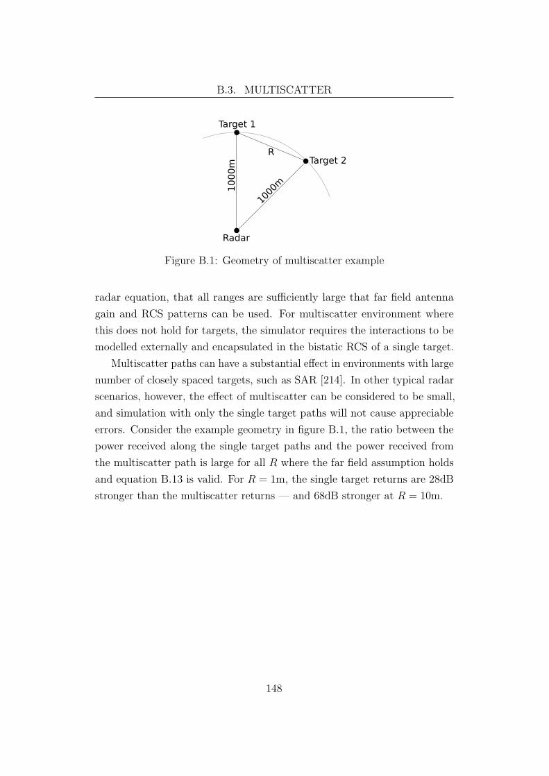
B.3. MULTISCATTER
Figure B.1: Geometry of multiscatter example
radar equation, that all ranges are sufficiently large that far field antenna
gain and RCS patterns can be used. For multiscatter environment where
this does not hold for targets, the simulator requires the interactions to be
modelled externally and encapsulated in the bistatic RCS of a single target.
Multiscatter paths can have a substantial effect in environments with large
number of closely spaced targets, such as SAR [214]. In other typical radar
scenarios, however, the effect of multiscatter can be considered to be small,
and simulation with only the single target paths will not cause appreciable
errors. Consider the example geometry in figure B.1, the ratio between the
power received along the single target paths and the power received from
the multiscatter path is large for all R where the far field assumption holds
and equation B.13 is valid. For R = 1m, the single target returns are 28dB
stronger than the multiscatter returns — and 68dB stronger at R = 10m.
148

References
[1] T. Balz, “Real-time SAR simulation on graphics processing units,” in
EUSAR 2006: 6th European Conference on Synthetic Aperture Radar,
2006.
[2] R. Lengenfelder, “The design and implementation of a radar simulator,”
Master’s thesis, University of Cape Town, Sep. 1998.
[3] D. B. Leeson and G. F. Johnson, “Short-term stability for a doppler
radar: Requirements, measurements and techniques,” Proceedings of
the IEEE, vol. 54, pp. 244–248, Feb. 1966.
[4] J. R. Vig, “Quartz crystal resonators and oscillators for frequency control
and timing applications: A tutorial,” U.S. Army Communications-
Electronics Command, Jan. 2000.
[5] “A guide to understanding and characterizing timing jitter,” Tektronix,
Inc., http://www.tektronix.com/jitter/, Tech. Rep., 2003.
[6] M. Brooker and M. Inggs, “Efficient generation of fα noise sequences
for radar simulation,” Submitted to IEEE Transactions on Aerospace
Electronic Systems, 2007.
[7] J. Park, K. Muhammad, and K. Roy, “Efficient modeling of 1/fα noise
using multirate process,” IEEE Transactions on Computer-Aided Design
of Integrated Circuits and Systems, vol. 25, no. 7, pp. 1247–1256, Jul.
2006.
[8] Maxim DS4026 10MHz to 51.84MHz TCXO, Dallas Semiconductor,
2007.
149

REFERENCES
[9] J. A. Scheer, “Timing jitter effects,” in Coherent Radar Performance
Estimation, J. A. Scheer and J. L. Kurtz, Eds. Artech House, 1993,
ch. 4.
[10] J. M. Horrell, “Range-doppler synthetic aperture radar processing at
vhf frequencies,” Ph.D. dissertation, University of Cape Town, May
1999.
[11] H. D. Griffiths, “Bistatic and multistatic radar,” University College
London, Tech. Rep., 2002.
[12] J. Meyer-Hilberg, “Pirdis: A new versatile tool for SAR/MTI systems
simulation,” in EUSAR 2006: 6th European Conference on Synthetic
Aperture Radar, 2006.
[13] L. Sevgi and A. S. Tanal, “Surface wave HF radar simulator,” in IEEE
Radar 1997, 1997.
[14] R. R. Boothe, “A digital computer program for determining the per-
formance of an aquisition radar through application of radar detection
probability theory,” U. S. Army Missile Command, Redstone Arsenal,
Report RD-TR-64-2, Dec. 1964.
[15] P. J. Golda, “Software simulation of synthetic aperture radar,” Master’s
thesis, University of Cape Town, 1997.
[16] G. Franceschetti, M. Migliaccio, D. Riccio, and G. Shirinzi, “SARAS: a
synthetic aperture radar (SAR) raw signal simulator,” IEEE Transac-
tions on Geoscience and Remote Sensing, vol. 30, no. 1, pp. 110–123,
Jan. 1992.
[17] G. Franceschetti, A. Iodice, D. Riccio, and G. Ruello, “A 2-D Fourier
domain approach for spotlight SAR raw signal simulation of extended
scenes,” in 2002 IEEE Internation Geoscience and Remote Sensing
Symposium, 2002, pp. 853–855.
150
REFERENCES
[18] C. Capsoni and M. D’Amicio, “A physically based radar simulator,”
Journal of Atmospheric and Oceanic Technology, vol. 15, no. 2, pp.
593–598, Apr. 1998.
[19] F. Xu and Y.-Q. Jin, “Imaging simulation of polarimetric sar for a com-
prehensive terrain scene using the mapping and projection algorithm,”
IEEE Transactions on Geoscience and Remote Sensing, vol. 44, no. 11,
pp. 3219–3234, Nov. 2006.
[20] J. F. Nouvel, A. Herique, W. Kofman, and A. Safaeinili, “Marsis radar
signal simulation,” in 2003 IEEE International Geoscience and Remote
Sensing Symposium, 2003. IGARSS ’03. Proceedings., vol. 4, Jul. 2003,
pp. 2756–2758.
[21] X. Xu and P. Huang, “A new RCS statistical model of radar targets,”
IEEE Transactions on Aerospace and Electronic Systems, vol. 33, no. 2,
pp. 710–714, Apr. 1997.
[22] ISO 9241-11:1998: Ergonomic requirements for office work with visual
display terminals (VDTs) – Part 11: Guidance on usability. Interna-
tional Organization for Standardization, 1998.
[23] ISO/IEC 14882:2003: Programming languages – C++. International
Organization for Standardization, 2003.
[24] G. E. Moore, “Cramming more components onto integrated circuits,”
Electronics, vol. 38, no. 8, pp. 1–4, 1965.
[25] J. D. Jackson, Classical Electrodynamics, 3rd ed. Wiley, 1999.
[26] S. Kingsley and S. Quegan, Understanding Radar Systems. SciTech
Publishing, 1999.
[27] J. G. Proakis and D. G. Manolakis, Digital Signal Processing: Principles,
Algorithms and Applications. Prentice Hall, 1996.
[28] C. E. Shannon, “A mathematical theory of communication,” Bell System
Technical Journal, vol. 27, pp. 379–423,623–656, 1948.
151

REFERENCES
[29] A. V. Oppenheim, R. W. Schafer, and J. R. Buck, Discrete-Time Signal
Processing, 2nd ed. Prentice Hall, 1999.
[30] V. A. Kotelnikov, “On the transmission capacity of the ether and of ca-
bles in electrical communications,” in Proceedings of the first All-Union
Conference on the technological reconstruction of the communications
sector and the development of low-current engineering, 1933, translation
by C C Bissel and V E Katsnelson.
[31] B. M. Oliver, J. Pierce, and C. E. Shannon, “The philosophy of PCM,”
Proceedings of the Institute of Radio Engineers, vol. 36, pp. 1324–1331,
Nov. 1948.
[32] W. R. Bennett, “Spectra of quantized signals,” Bell System Technical
Journal, vol. 27, pp. 446–472, 1948.
[33] R. M. Gray and D. L. Neuhoff, “Quantization,” IEEE Transactions on
Information Theory, vol. 44, no. 6, pp. 2325–2384, Oct. 1998.
[34] J. A. Scheer, “A/D conversion effects,” in Coherent Radar Performance
Estimation, J. A. Scheer and J. L. Kurtz, Eds. Artech House, 1993,
ch. 5.
[35] J. D. Echard and M. L. Watt, “The quantization noise spectrum of
a sinusoid on colored noise,” IEEE Transactions on Acoustics, Speech
and Signal Processing, vol. 39, no. 8, pp. 1780–1787, Aug. 1991.
[36] IEEE Std 754-1984: Standard for Binary Floating-Point Arithmetic.
The Institute of Electrical and Electronics Engineers, Inc., 1985.
[37] F. Hartwig and A. Lacroix, “The properties of floating point single
quantization including under- and overflow,” in Proceedings of the 1996
European Signal Processing Conference, 1996.
[38] R. Dunay, I. Kollar, and B. Widrow, “Dithering for floating-point num-
ber representation,” in 1st International Online Workshop on Dithering
in Measurement, Mar. 1998.
152
REFERENCES
[39] W. S. Brown, “A simple but realistic model of floating-point computa-
tion,” ACM Transactions on Mathematical Software (TOMS), vol. 7,
no. 4, pp. 445–480, Dec. 1981.
[40] D. Goldberg, “What every computer scientist should know about float-
ing point,” ACM Computing Surveys, vol. 23, no. 1, pp. 5–48, Mar.
1991.
[41] E. Hecht, Optics, 4th ed. Addison-Wesley, 2002.
[42] R. C. Jones, “New calculus for the treatment of optical systems,” Journal
of the Optical Society of America, vol. 31, pp. 488–493, 1941.
[43] ——, “A new calculus for the treatment of optical systems II: Proof of
three general equivalence theorems,” Journal of the Optical Society of
America, vol. 31, pp. 493–, 1941.
[44] ——, “New calculus for the treatment of optical systems VIII: Electro-
magnetic theory,” Journal of the Optical Society of America, vol. 46,
pp. 126–, 1956.
[45] M. C. Jackson, “The geometry of bistatic radar systems,” IEE Proceed-
ings, Part F, vol. 133, pp. 604–612, Dec. 1986.
[46] “DoD world geodetic system 1984: Its definition and relationships with
local geodetic systems,” National Geospatial-Intelligence Agency, Tech.
Rep. TR8350.2, Jun. 2004.
[47] V. S. Chernyak, Fundamentals of Multisite Radar Systems. Gordon
and Breach Scientific Publishers, 1998.
[48] N. J. Willis, “Bistatic radar,” in Radar Handbook, 2nd ed., M. I. Skolnik,
Ed. McGraw-Hill, 1990, ch. 25.
[49] ISO 31-5: Quantities and units: Electricity and Magnetism. Interna-
tional Organization for Standardization, 1992.
[50] D. Barton, Modern Radar System Analysis. Artech House, Inc, 1988.
153

REFERENCES
[51] M. I. Skolnik, Introduction to Radar Systems, 2nd ed. McGraw-Hill,
2001.
[52] P. Swerling, “Detection of fluctuating pulsed signals in the presence of
noise,” Transactions of the IRE, vol. IT-3, pp. 175–178, 1957.
[53] J. I. Marcum and P. Swerling, “Studies of target detection by pulsed
radar,” IRE Transactions on Information Theory, vol. IT-6, p. 2, Apr.
1960.
[54] P. Swerling, “Probability of detection for fluctuating targets,” IEEE
Transactions on Information Theory, vol. 6, no. 2, pp. 269–308, Apr.
1960.
[55] S. L. Johnston, “Target fluctuation models for radar system design and
performance analysis: An overview of three papers,” IEEE Transactions
on Aerospace and Electronic Systems, vol. 33, no. 2, pp. 696–670, Apr.
1997.
[56] ——, “Target model pitfalls (illness, diagnosis and prescription),” IEEE
Transactions on Aerospace and Electronic Systems, vol. 33, no. 2, pp.
715–720, Apr. 1997.
[57] P. Swerling, “Radar probability of detection for some additional fluc-
tuating target cases,” IEEE Transactions on Aerospace and Electronic
Systems, vol. 33, no. 2, pp. 698–709, Apr. 1997.
[58] W. W. Weinstock, “Target cross section models for radar systems
analysis,” Ph.D. dissertation, University of Pennsylvania, 1956.
[59] D. A. Shnidman, “Expanded Swerling target models,” IEEE Transac-
tions on Aerospace and Electronic Systems, vol. 39, no. 3, pp. 1059–1069,
Jul. 2003.
[60] P. Z. Peebles, Probability, Random Variables and Random Signal Prin-
ciples, 4th ed. McGraw Hill, 2001.
154

REFERENCES
[61] M. Abramowitz and I. A. Stegun, The Handbook of Mathematical
Functions. Dover Publications, 1965.
[62] W. H. Press, S. A. Teukolsky, W. T. Vetterling, and B. P. Flannery,
Numerical Recipes in C: The Art of Scientific Computing. Cambridge
University Press, 1992.
[63] J. K. Jao and M. Elbaum, “First-order statistics of a non-Rayleigh
fading singal and its detection,” Proceedings of the IEEE, vol. 66, pp.
781–789, Jul. 1978.
[64] G. R. Heidbreder and R. L. Mitchell, “Detection probabilies for log-
normally distributed signals,” IEEE Transactions on Aerospace and
Electronic Systems, vol. 3, pp. 5–13, Jan. 1967.
[65] G. E. Pollon, “Statistical parameters for scattering from randomly
orientated arrays,” IEEE Transactions on Antennas and Propagation,
vol. 18, pp. 68–75, Jan. 1970.
[66] J. D. Wilson, “Probability of detecting aircraft targets,” IEEE Trans-
actions on Aerospace Electronic Systems, vol. 8, pp. 757–761, 1972.
[67] P. E. Hudson, “Passive multistatic radars in anti-stealth air defence,”
Master’s thesis, Canadian Forces College, 2003. [Online]. Available:
http://wps.cfc.forces.gc.ca/papers/csc/csc29/mds/hudson.pdf
[68] E. F. Knott, J. F. Shaeffer, and M. T. Tuley, Radar Cross Section,
2nd ed. Artech House, 1993.
[69] J. I. Glaser, “Some results in the bistatic radar cross section (RCS) of
complex objects,” Proceedings of the IEEE, vol. 77, no. 5, pp. 639–648,
May 1989.
[70] R. E. Kell, “On the derivation of bistatic RCS from monostatic mea-
surements,” Proceedings of the IEEE, vol. 53, no. 8, pp. 983–987, Aug.
1965.
155

REFERENCES
[71] M. W. Long, Radar Reflectivity of Land and Sea, 2nd ed. Artech
House, Inc., 1983.
[72] J. H. Huynen, “Phenomenological theory of radar targets,” in Electro-
magnetic Scattering, L. E. Uslenghi, Ed. Academic Press, New York,
1978.
[73] I. M. Yaglom, Geometric Transformations I. Random House, 1962.
[74] P. J. Mohr and B. N. Taylor, “CODATA recommended values of the
fundamental physical constants: 2002,” Reviews of Modern Physics,
vol. 77, pp. 1–107, 2005.
[75] S. R. Doughty, “Development and performance evaluation of a multi-
static radar system,” Ph.D. dissertation, University College London,
Jul. 2008.
[76] T. E. Derham, S. Doughty, K. Woodbridge, and C. J. Baker, “Design
and evaluation of a low-cost multistatic netted radar system,” IET
Radar, Sonar and Navigation, vol. 1, no. 5, pp. 362–368, Oct. 2007.
[77] S. Doughty, K. Woodbridge, and C. Baker, “Characterisation of a
multistatic radar system,” in Radar Conference, 2006. 3rd European,
2006.
[78] S. R. Doughty, “Multistatic radar measurements and development,”
Master’s thesis, University College London, Dec. 2005.
[79] Y. Paichard, J. Castelli, P. Dreuillet, and G. Bobillot, “HYCAM: A
RCS measurement and analysis system for time-varying targets,” in
Instrumentation and Measurement Technology Conference, 2006. IMTC
2006. Proceedings of the IEEE, Apr. 2006.
[80] R. Buderi, The invention that changed the world: the story of radar
from war to peace. Simon & Schuster, 1996.
[81] G. Brooker, “Long-range imaging radar for autonomous navigation,”
Ph.D. dissertation, University of Sydney, 2005.
156

REFERENCES
[82] A. Celliers, “The design of a 94GHz high resolution coherent radar,”
Ph.D. dissertation, University of Cape Town, 1987.
[83] P. Horowitz and W. Hill, The Art of Electronics. Cambridge University
Press, 1989.
[84] R. S. Raven, “Requirements on master oscillators for coherent radar,”
Proceedings of the IEEE, vol. 54, pp. 237–243, 1966.
[85] J. C. Kirk, “Bistatic SAR motion compensation,” in IEEE International
Radar Conference, 1985.
[86] C. J. Baker and A. L. Hume, “Netted radar sensing,” IEEE aerosp.
electron. syst. mag., vol. 18, no. 2, pp. 3–6, Feb. 2003.
[87] A. L. Hume and C. J. Baker, “Netted radar sensing,” in Proceedings of
the 2001 IEEE Radar Conference, May 2001.
[88] E. J. Baghdady, R. N. Lincoln, and B. D. Nelin, “Short-term frequency
stability: Characterization, theory and measurement,” Proceedings of
the IEEE, vol. 53, pp. 704–722, 1965.
[89] J. A. Barnes, A. R. Chi, L. S. Cutler, D. J. Healey, D. B. Leeson, T. E.
McGunigal, J. A. Mullen, W. L. Smith, and R. L. Sydnor, “Characteri-
zation of frequency stability,” National Bureau of Standards, Technical
Note 394, Oct. 1970.
[90] ——, “Characterization of frequency stability,” IEEE Transactions on
Instrumentation and Measurement, vol. IM-20, pp. 105–120, May 1971.
[91] T. Walter, “Characterizing frequency stability: A continuous power-law
model with discrete sampling,” IEEE Transactions on Instrumentation
and Measurement, vol. 43, no. 1, pp. 69–79, Feb. 1994.
[92] D. W. Allan, “Time and frequency (time-domain) characterization,
estimation and prediction of precision clocks and oscillators,” IEEE
Transactions on Ultrasonics, Ferroelectrics and Frequency Control, vol.
UFFC-34, no. 6, pp. 647–654, Nov. 1987.
157

REFERENCES
[93] W. Davenport and W. Root, Random Signals and Noise. McGraw-Hill,
1958.
[94] L. S. Cutler and C. L. Searle, “Some aspects of the theory and measure-
ment of frequency fluctuations in frequency standards,” Proceedings of
the IEEE, vol. 54, pp. 135–154, Feb. 1966.
[95] J. A. Barnes, “Atomic timekeeping and statistics of precision signal
generators,” Proceedings of the IEEE, vol. 54, pp. 207–220, Feb. 1966.
[96] IEEE Std 1139-1999: IEEE standard definitions of physical quantities
for fundamental frequency and time metrology - random instabilities.
The Institute of Electrical and Electronics Engineers, Inc., 1999.
[97] G. W. Ewell, “Stability and stable sources,” in Coherent Radar Perfor-
mance Estimation, J. A. Scheer and J. L. Kurtz, Eds. Artech House,
1993, ch. 2.
[98] HF Ultra Low Noise OCXO, Wenzel Associates, Inc., 2006.
[99] J. Bendat and A. Piersol, Random Data: Analysis and Measurement
Procedures. Wiley-Interscience, 1986.
[100] G. Samorodnitsky, “Long range dependence,” in Encyclopedia of Actu-
arial Science, J. L. Teugels and B. Sundt, Eds. John Wiley & Sons,
Ltd., 2004, vol. 2, pp. 1033–1036.
[101] G. Lindgren, “Stationary processes,” in Encyclopedia of Actuarial Sci-
ence, J. L. Teugels and B. Sundt, Eds. John Wiley & Sons, Ltd., 2004,
vol. 3, pp. 1589–1593.
[102] D. Howe, D. Allan, and J. Barnes, “Properties of signal sources and
measurement methods,” in Thirty Fifth Annual Frequency Control
Symposium, 1981, pp. 669–716.
[103] J. A. Barnes, R. H. Jones, P. V. Tryon, and D. W. Allan, “Stochastic
models for atomic clocks,” in NASA. Goddard Space Flight Center
158
REFERENCES
Proc. of the 14th Ann. Precise Time and Time Interval (PTTI) Appl.
Planning Meeting, Feb. 1983.
[104] D. W. Allan and J. A. Barnes, “A modified ’Allan variance’ with
increased oscillator characterization ability,” in Thirty Fifth Annual
Frequency Control Symposium, 1981, pp. 470–475.
[105] D. A. Howe, “The total deviation approach to long-term characterization
of frequency stability,” IEEE Transactions on Ultrasonics, Ferroelectrics,
and Frequency Control, vol. 47, pp. 1102–1109, 2000.
[106] C. A. Greenhall, D. A. Howe, and D. B. Percival, “Total variance,
an estimator of long-term frequency stability,” IEEE Transactions on
Ultrasonics, Ferroelectrics, and Frequency Control, vol. 46, no. 5, pp.
1183–1191, Sep. 1999.
[107] C. A. Greenhall, “Spectral ambiguity of Allan variance,” IEEE Transac-
tions on Instrumentation and Measurement, vol. 47, no. 3, pp. 623–627,
Jun. 1998.
[108] ITU-T, “Definitions and terminology for synchronization networks,”
International Telecommunication Union, Standard G.810, Aug. 1996.
[109] N. Roberts, “Phase noise and jitter — a primer for digital designers,”
Zarlink Semiconductor, Tech. Rep., 2003.
[110] W. Kester, “Converting oscillator phase noise to time jitter,” Analog
Devices, Application Note MT-008, 2005.
[111] A. Einstein, “Method for the determinination of the statistical values
of observations concerning quantities subject to irregular fluctuations,”
IEEE ASSP Magazine, vol. 4, no. 4, p. 6, Oct. 1987.
[112] C. A. Greenhall, “FFT-based methods for simulating flicker FM,” in
34th Annual Precise Time and Time Interval (PTTI) Meeting, Dec.
2002, pp. 481–491.
159

REFERENCES
[113] N. J. Kasdin, “Discrete simulation of colored noise and stochastic
processes and 1/f power law noise generation,” Proceedings of the IEEE,
vol. 83, no. 5, pp. 802–827, May 1995.
[114] E. Milotti, “Exact numerical simulation of power-law noises,” Physical
Review E, vol. 72, no. 5, p. 056701, 2005.
[115] S. Plaszczynski, “Generating long streams of 1/fα noise,” Fluctuation
and Noise Letters, vol. 7, no. 1, pp. R1–R13, 2007.
[116] J. Nagler and J. Claussen, “1/fa spectra in elementry cellular automata
and fractal signals,” Physical Review E, vol. 71, p. 067103, 2005.
[117] J. C. Claussen, J. Nagler, and H. G. Schuster, “Sierpinski signal gener-
ates 1/fα spectra,” Physical Review E, vol. 70, pp. 032 101–1, 2004.
[118] Y. Meyer, F. Sellan, and M. S. Taqqu, “Wavelets, generalized white
noise and fractional integration: The synthesis of fractional brownian
motion,” The Journal of Fourier Analysis and Applications, vol. 5, no. 5,
pp. 465–494, 1999.
[119] E. J. McCoy and A. T. Walden, “Wavelet analysis and synthesis of sta-
tionary long-memory processes,” Journal of Computational and Graph-
ical Statistics, vol. 5, no. 1, pp. 26–56, Mar. 1996.
[120] P. Flandrin, “Wavelet analysis and synthesis of fractional Brownian
motion,” IEEE Transactions on Information Theory, vol. 38, no. 2, pp.
910–917, Mar. 1992.
[121] J. R. M. Hosking, “Fractional differencing,” Biometrika, vol. 68, no. 1,
pp. 165–176, Apr. 1981.
[122] R. Whittle, “DSP generation of pink noise,”
http://www.firstpr.com.au/dsp/pink-noise/, Tech. Rep., 2007.
[123] B. Friedlander and B. Porat, “The modified Yule-Walker method of
ARMA spectral estimation,” IEEE Transactions on Aerospace and
Electronic Systems, vol. AES-20, no. 2, pp. 158–173, Mar. 1984.
160

REFERENCES
[124] I. W. Selesnick, M. Lang, and C. S. Burrus, “Magnitude squared design
of recursive filters with the chebyshevnorm using a constrained rational
Remez algorithm,” in Sixth IEEE Digital Signal Processing Workshop,
1994.
[125] A. Rodriguez and S. G. Johnson, “Efficient generation of correlated
random numbers using chebyshev-optimal magnitude-only IIR filters,”
Mar. 2007, eprint arXiv:physics/0703152.
[126] P. Thajchayapong and P. Rayner, “Recursive digital filter design by
linear programming,” IEEE Transactions on Audio and Electroacoustics,
vol. 21, no. 2, pp. 107–112, Apr. 1973.
[127] L. R. Rabiner, N. Y. Graham, and H. D. Helms, “Linear programming
design of IIR digital filters with arbitrary magnitude function,” IEEE
Transactions on Acoustics, Speech, And Signal Processing, vol. 22, no. 2,
pp. 117–123, Apr. 1974.
[128] D. E. Dudgeon, “Recursive filter design using differential correction,”
IEEE Transactions on Acoustics, Speech, and Signal Processing, vol. 22,
no. 6, pp. 443–448, Dec. 1974.
[129] I. Barrodale, M. Powell, and F. Roberts, “The differential correction
algorithm for rational l∞ approximation,” SIAM Journal of Numerical
Analysis, vol. 9, pp. 493–504, 1972.
[130] X. Zhang, K. Suzuki, and T. Yoshikawa, “Complex chebyshev approx-
imation for IIR digital filters based on eigenvalue problem,” IEEE
Transactions on Circuits and Systems II, vol. 47, no. 12, pp. 1429–1436,
Dec. 2000.
[131] X. Zhang and H. Iwakura, “Design of IIR digital filters based on
eigenvalue problem,” IEEE Transactions on Signal Processing, vol. 44,
no. 6, pp. 1325–1333, Jun. 1996.
[132] P. P. Vaidyanathan, Multirate Systems and Filter Banks. Prentice
Hall, 1992.
161

REFERENCES
[133] R. Crochiere and L. Rabiner, Multirate Digital Signal Processing.
Prentice-Hall, 1983.
[134] R. W. Hamming, Digital Filters, 3rd ed. Dover Publications, Inc.,
1999.
[135] T. W. Parks and C. S. Burrus, Digital Filter Design. Wiley, New York,
1987.
[136] M. A. Lombardi, “Fundamentals of time and frequency,” in The Mecha-
tronics Handbook, R. H. Bishop, Ed. CRC Press, 2002, ch. 17.
[137] W. J. Riley and C. A. Greenhall, “Power law noise identification using
the lag 1 autocorrelation,” in 18th European Frequency and Time Forum,
2004.
[138] R. T. Austin, A. W. England, and G. H. Wakefield, “Special problems
in the estimation of power-law spectra as applied to topographical
modeling,” IEEE Transactions on Geoscience and Remote Sensing,
vol. 32, no. 4, pp. 928–939, Jul. 1994.
[139] J. Capon, “High-resolution frequency-wavenumber spectrum analysis,”
Proceedings of the IEEE, vol. 57, pp. 1408–1418, 1969.
[140] P. D. Welch, “The use of the fast Fourier transform for the estimation
of power spectra: A method base on time averaging over short, modified
periodograms,” IEEE Transactions on Audio and Electroacoustics, vol.
AU-15, pp. 70–73, Jun. 1967.
[141] S. M. Kay, Modern Spectral Estimation. Prentice Hall, 1988.
[142] B. B. Mandelbrot and J. W. V. Ness, “Fractional brownian motions,
fractional noises and applications,” SIAM Review, vol. 10, no. 4, pp.
422–436, Oct. 1968.
[143] J. Weidendorfer, M. Kowarschik, and C. Trinitis, “A tool suite for
simulation based analysis of memory access behavior,” in Proceedings
162

REFERENCES
of the 4th International Conference on Computational Science (ICCS
2004), Jun. 2004.
[144] W. V. Shrader and V. Gregers-Hansen, “MTI radar,” in Radar Handbook,
2nd ed., M. I. Skolnik, Ed. McGraw-Hill, 1990, ch. 15.
[145] R. R. Kerr, “MTI systems,” in Coherent Radar Performance Estimation,
J. A. Scheer and J. L. Kurtz, Eds. Artech House, 1993, ch. 8.
[146] J. A. Scheer, “Introduction to coherent radar systems,” in Coherent
Radar Performance Estimation, J. A. Scheer and J. L. Kurtz, Eds.
Artech House, 1993, ch. 1.
[147] J. A. Scheer and J. L. Kurtz, Eds., Coherent Radar Performance
Estimation. Artech House, 1993.
[148] F. G. Stremler, Introduction to Communication Systems, 3rd ed. Ad-
dison Wesley, 1992.
[149] M. L. Belcher and G. V. Morris, “Pulsed doppler radar,” in Coherent
Radar Performance Estimation, J. A. Scheer and J. L. Kurtz, Eds.
Artech House, 1993, ch. 9.
[150] J. Steensgaard-Madsen, “High-performance data converters,” Ph.D.
dissertation, The Technical University of Denmark, 1999.
[151] P. Smith, “Little known characteristics of phase noise,” Analog Devices,
Application Note AN-741, 2004.
[152] GNU, “The GNU General Public Licence,”
http://www.gnu.org/licenses/gpl.html, June 1991.
[153] G. van Rossum, Python Reference Manual, 2nd ed., Python Software
Foundation, http://docs.python.org/ref/ref.html, Feb. 2008.
[154] B. Stroustrup, The C++ Programming Language, 3rd ed. Addison-
Wesley, 1997.
[155] S. Meyers, Effective C++, 3rd ed. Addison-Wesley, 2005.
163

REFERENCES
[156] “Boost C++ libraries,” http://www.boost.org/.
[157] “The computer language benchmarks game,”
http://shootout.alioth.debian.org/, accessed March 2008.
[158] “Tiobe programming community in-
dex for March 2008,” TIOBE Software,
http://www.tiobe.com/index.php/content/paperinfo/tpci/index.html,
Tech. Rep., Mar. 2008, accessed March 2008.
[159] H. E. Hinnant, B. Dawes, L. Crowl, J. Garland, and A. Williams,
“Multi-threading library for standard C++,” ISO JTC1/SC22/WG21
- The C++ Standards Committee, http://www.open-
std.org/jtc1/sc22/wg21/docs/papers/2007/n2320.html, Tech. Rep.
N2320, Jun. 2007.
[160] N. M. Josuttis, The C++ Standard Library: A Tutorial and Reference.
Addison-Wesley, 1999.
[161] S. Meyers, Effective STL. Addison-Wesley, 2001.
[162] SD15 2.4GHz Parabolic antenna, Stella Doradus Ireland Ltd., data
Sheet.
[163] E. Dijkstra, “Over sienpalen (EWD 74) (Dutch),”
http://www.cs.utexas.edu/users/EWD/ewd00xx/EWD74.PDF.
[164] A. B. Downey, The Little Book of Semaphores. Green Tea Press, 2008.
[165] N. Nethercote and J. Seward, “Valgrind: A framework for heavyweight
dynamic binary instrumentation,” in Proceedings of ACM SIGPLAN
2007 Conference on Programming Language Design and Implementation,
Jun. 2007.
[166] N. Nethercote, “Dynamic binary analysis and instrumentation,” Ph.D.
dissertation, University of Cambridge, Nov. 2004.
164

REFERENCES
[167] A. S. Tanenbaum, Structured Computer Organization, 4th ed. Prentice
Hall, 1999.
[168] A. H. Karp and H. P. Flatt, “Measuring parallel processor performance,”
Communications of the ACM, vol. 33, no. 5, pp. 539–543, May 1990.
[169] J. Dean and S. Ghemawat, “Mapreduce: Simplified data processing
on large clusters,” in OSDI’04: Sixth Symposium on Operating System
Design and Implementation,, 2004, pp. 137–150.
[170] G. E. Revesz, Lambda Calculus, Combinators, and Functional Program-
ming. Cambridge University Press, 1988.
[171] G. Michaelson, An Introduction to Functional Programming through
Lambda Calculus. Addison-Wesley, 1989.
[172] J. Dean and S. Ghemawat, “Mapreduce: Simplified data processing
on large clusters,” Communications of the ACM, vol. 51, no. 1, pp.
107–113, Jan. 2008.
[173] C. Ranger, R. Raghuraman, A. Penmetsa, G. Bradski, and C. Kozyrakis,
“Evaluating mapreduce for multi-core and multiprocessor systems,” in
High Performance Computer Architecture, 2007. HPCA 2007. IEEE
13th International Symposium on, 2007, pp. 13–24.
[174] M. D. Linderman, J. D. Collins, H. Wang, and T. H. Meng, “Merge: a
programming model for heterogeneous multi-core systems,” in Proceed-
ings of the 13th international conference on Architectural support for
programming languages and operating systems, 2008, pp. 287–296.
[175] T. I. Laakso, V. Vlimki, M. Karjalainen, and U. K. Laine, “Splitting
the unit delay - tools for fractional delay filter design,” IEEE Signal
Processing Magazine, vol. 13, no. 1, pp. 30–60, Jan. 1996.
[176] V. Valimaki and T. I. Laakso, “Fractional delay filters — design and
applications,” in Theory and Applications of Nonuniform Sampling,
F. Marvasti, Ed. Kluwer, 2000.
165

REFERENCES
[177] L. R. Rabiner and B. Gold, Theory and Application of Digital Signal
Processing. Prentice-Hall, 1975.
[178] V. Valimaki and T. I. Laakso, “Principles of fractional delay filters,”
in IEEE International Conference on Acoustics, Speech and Signal
Processing. IEEE, Jun. 2000.
[179] A. Yardim, G. Cain, and P. Henry, “Optimal two-term offset windowing
for fractional delay,” Electronics Letters, vol. 32, no. 6, pp. 526–527,
Mar. 1996.
[180] G. Cain, A. Yardim, and P. Henry, “New FIR fractional delayors for
effective signal interpolation,” in Proc. DSP’94 ESA Workshop on DSP
for Space Applications, Sep. 1994, pp. 42–49.
[181] ——, “Offset windowing for FIR fractional-sample delay,” in Proc.
ICASSP’95, May 1995, pp. 1276–1279.
[182] J. O. Smith and P. Gossett, “A flexible sampling-rate conversion
method,” in Proceedings of the International Conference on Acous-
tics, Speech, and Signal Processing, vol. 2, Mar. 1984, pp. 19.4.1–19.4.2.
[183] J. O. Smith, Digital Audio Resampling Home Page. http://www-
ccrma.stanford.edu/˜jos/resample/, Jan. 2002.
[184] J. F. Kaiser, “Using the I0 sinh window function,” IEEE Transactions
on Circuits and Systems, vol. 22, pp. 20–23, 1974.
[185] J. Kaiser and R. Schafer, “On the use of the i0-sinh window for spec-
trum analysis,” IEEE Transactions on Acoustics, Speech, and Signal
Processing, vol. 28, no. 1, pp. 105–107, Feb. 1980.
[186] J. F. Kaiser, “Digital filters,” in System Analysis by Digital Computer,
F. F. Kuo and J. F. Kaiser, Eds. Wiley, 1966, pp. 218–285.
[187] D. Slepian, H. O. Pollack, and H. J. Landau, “Prolate spheroidal wave
functions, Fourier analysis and uncertainty,” Bell Systems Technical
Journal, vol. 40, pp. 43–63, Jan. 1961.
166

REFERENCES
[188] C. W. Farrow, “A continuously variable digital delay element,” in
Circuits and Systems, 1988., IEEE International Symposium on, vol. 3,
Jun. 1988, pp. 2641–2645.
[189] J. Radatz, Ed., IEEE Standard dictionary of electrical and electronics
terms, 6th ed. Institute of Electrical and Electronics Engineers, 1997.
[190] L. J. Cutrona, “Synthetic aperture radar,” in Radar Handbook, 2nd ed.,
M. I. Skolnik, Ed. McGraw-Hill, 1990, ch. 15.
[191] J. C. Curlander and R. N. McDonough, Synthetic Aperture Radar:
Systems and Signal Processing. Wiley, 1991.
[192] M. R. Inggs, “First results from the South African VHF imaging radar,”
in Proceedings of the 3rd IMACS/IEEEE International Multiconference
on Circuits, Systems, Communications and Computers, Jul. 1999.
[193] M. R. Inggs, J. M. Horrell, A. Knight, and P. G. Koeppen, “iSAR: A
multispectral polarimetric airborne SAR system,” in Proceedings of the
1994 Internation Geoscience and Remote Sensing Symposium, vol. 4,
Aug. 1994, pp. 2237–2239.
[194] R. T. Lord, “Aspects of stepped-frequency processing for low-frequency
SAR systems,” Ph.D. dissertation, University of Cape Town, Feb. 2000.
[195] H. D. Griffiths and C. J. Baker, “Passive coherent location radar systems.
part 1: Performance prediction,” IEE Proceedings on Radar, Sonar and
Navigation, vol. 152, pp. 153–159, 2005.
[196] P. E. Howland, D. Maksimiuk, and G. Reitsma, “Fm radio based bistatic
radar,” IEEE Proceedings on Radar, Sonar and Navigation, vol. 152,
pp. 107–115, 2005.
[197] J. Baniak, G. Baker, A. Cunningham, and L. Martin, “Silent sentry
passive surveillance,” Aviation week and space technology, Jun. 1999.
167

REFERENCES
[198] Z. Jiabing, T. Liang, and H. Yi, “Adaptive beamforming passive radar
based on fm radio transmitter,” in CIE ’06 International Conference
on Radar, Oct. 2006, pp. 1–4.
[199] J. D. Sahr and F. D. Lind, “The manastash ridge radar: A passive
bistatic radar for upper atmospheric radio science,” Radio Science,
vol. 32, no. 6, pp. 2345–2358, 1997.
[200] P. E. Howland, “Target tracking using television-based bistatic radar,”
IEE Proceedings on Radar, Sonar and Navigation, vol. 146, no. 3, pp.
166–174, 1999.
[201] H. D. Griffiths and N. R. Long, “Television-based bistatic radar,” IEE
Proceedings, Part F, vol. 133, no. 7, pp. 649–657, Dec. 1986.
[202] H. Sun, D. K. P. Tan, and Y. Lu, “Design and implementation of an
experimental gsm based passive radar,” in Proceedings of the IEEE
International Radar Conference, 2003, pp. 418–422.
[203] H. D. Griffiths, C. J. Baker, J. Baubert, N. Kitchen, and M. Treagust,
“Bistatic radar using satellite-borne illuminators,” in Proceedings of the
IEEE International Radar Conference, 2002.
[204] C. J. Baker, H. D. Griffiths, and I. Papoutsis, “Passive coherent location
radar systems. part 2: Waveform properties,” IEE Proceedings on Radar,
Sonar and Navigation, vol. 152, no. 3, pp. 160–168, Jun. 2005.
[205] T. Derham, S. Doughty, K. Woodbridge, and C. Baker, “Realisation
and evaluation of a low cost netted radar system,” in Radar, 2006. CIE
’06. International Conference on, 2006.
[206] Piezotite Ultrasonic Sensor MA Series, muRata.
[207] J. B. Allen and L. R. Rabiner, “A unified approach to short-time Fourier
analysis and synthesis,” Proceedings of the IEEE, vol. 65, pp. 1558–1564,
Nov. 1977.
168
REFERENCES
[208] W. L. Patterson, “Advanced refractive effects prediction system
(AREPS),” in Radar Conference, 2007 IEEE, 2007.
[209] ——, “Advanced refractive effects prediction system (AREPS),” Space
and Naval Warfare Systems Center, San Diego, Research paper A242434,
Aug. 2001.
[210] P. Dutre, K. Bala, and P. Bekaert, Advanced Global Illumination. A
K Peters Ltd., 2006.
[211] M. Pharr and G. Humphreys, Physically Based Rendering : From
Theory to Implementation. Morgan Kaufmann, 2004.
[212] U. Jakobus, User’s Guide To FEKO, EM Software & Systems-SA (Pty)
Ltd.
[213] C. A. Greene and R. T. Moller, “The effect of normally distributed ran-
dom phase errors on synthetic array gain patterns,” IRE Transactions,
vol. MIL-6, pp. 119–121, Apr. 1962.
[214] D. L. Evans, T. G. Farr, J. P. Ford, T. W. Thompson, and C. L. Werner,
“Multipolarization radar images for geologic mapping and vegetation
discrimination,” IEEE Transactions on Geoscience and Remote Sensing,
vol. GE-24, no. 2, pp. 246–257, Mar. 1986.
169
Top Related