


Languages
Pages
Legal

QEDQueen’s Economics Department Working Paper No. 1363
The cointegrated vector autoregressive model with generaldeterministic terms
Søren JohansenUniversity of Copenhagen and CREATES
Morten Ørregaard NielsenQueen’s University and CREATES
Department of EconomicsQueen’s University
94 University AvenueKingston, Ontario, Canada
K7L 3N6
7-2016
The cointegrated vector autoregressive modelwith general deterministic terms
Søren Johansen∗
University of Copenhagenand CREATES
Morten Ørregaard Nielsen†
Queen’s Universityand CREATES
June 4, 2017
Abstract
In the cointegrated vector autoregression (CVAR) literature, deterministic termshave until now been analyzed on a case-by-case, or as-needed basis. We give a compre-hensive unified treatment of deterministic terms in the additive model Xt = γZt + Yt,where Zt belongs to a large class of deterministic regressors and Yt is a zero-meanCVAR. We suggest an extended model that can be estimated by reduced rank regres-sion, and give a condition for when the additive and extended models are asymptoticallyequivalent, as well as an algorithm for deriving the additive model parameters from theextended model parameters. We derive asymptotic properties of the maximum like-lihood estimators and discuss tests for rank and tests on the deterministic terms. Inparticular, we give conditions under which the estimators are asymptotically (mixed)Gaussian, such that associated tests are χ2-distributed.
Keywords: Additive formulation, cointegration, deterministic terms, extended model,likelihood inference, VAR model.
JEL Classification: C32.
1 IntroductionThe cointegrated vector autoregressive (CVAR) model continues to be one of the most com-monly applied models in many areas of empirical economics, as well as other disciplines.However, the formulation and modeling of deterministic terms in the CVAR model haveuntil now been analyzed only on a case-by-case basis because no general treatment exists.Moreover, the role of deterministic terms is not always intuitive and is often diffi cult tointerpret. Indeed, Hendry and Juselius (2001, p. 95) note that “In general, parameter infer-ence, policy simulations, and forecasting are much more sensitive to the specification of thedeterministic than the stochastic components of the VAR model.”
∗Corresponding author. Address: Department of Economics, University of Copenhagen, ØsterFarimagsgade 5, building 26, DK-1353, Copenhagen K, Denmark. Telephone: +45 35323071. Email:[email protected]†Email: [email protected]
1
The CVAR model with general deterministic terms 2
In this paper we give a comprehensive unified treatment of the CVAR model for a largeclass of deterministic regressors and derive the relevant asymptotic theory. There are twoways of modeling deterministic terms in the CVAR model, and we call these the additiveand innovation formulations. In the additive formulation, the deterministic terms are addedto the process, and in the innovation formulation they are added to the dynamic equations.
1.1 The additive formulation
In this paper, we analyze the additive formulation. To fix ideas, let the p-dimensional timeseries Xt be given by the additive model,
Haddr : Xt = Yt + γZt, t = 1− k, . . . ,−1, 0, . . . , T, (1)
Π(L)Yt = εt, t = 1, . . . , T,
where Zt is a multivariate deterministic regressor and
Π(z) = (1− z)Ip − αβ′z −k−1∑i=1
Γi(1− z)zi (2)
is the lag-polynomial defining the cointegrated I(1) process Yt. Furthermore, εt is i.i.d. (0,Ω),Y0, . . . , Y1−k are fixed initial values. We let π = (α, β,Γ1, . . . ,Γk−1) denote the parametersin Π(L) and let λ = (π, γ) with true value λ0 = (π0, γ0). Then λ consists of freely varyingparameters, where α, β are p × r for some r < p. Throughout, we will use the Gaussianlikelihood function to derive (quasi-) maximum likelihood estimators (MLEs), but as usual,asymptotic properties will not require normality. We also fix Ω = Ω0 at the true value, whichis without loss of generality in the asymptotic analysis of the remaining parameters becauseinference on Ω is asymptotically independent of inference on λ.The advantage of the formulation in (1) is that the role of the deterministic terms for the
properties of the process is explicitly modeled, and the interpretation is relatively straight-forward. One can, for example, focus on the mean of the stationary processes ∆Xt and β′Xt,for which we find from (1) that
E(∆Xt) = γ∆Zt and E(β′Xt) = β′γZt. (3)
Thus, γ can be interpreted as a “growth rate”, and, moreover, β′γ can be more accuratelyestimated than the rest of γ, because the information
∑Tt=1 ZtZ
′t in general is larger than∑T
t=1 ∆Zt∆Z′t. Note that if Zt contains the constant with parameter γ1 ∈ Rp, then the
corresponding entry in ∆Zt is zero and does not contain information about γ1, and we cantherefore only identify β′γ1.When analyzing properties of the process, the following I(1) conditions are important,
see Johansen (1996, Theorem 4.2). Here, and throughout, for any p × s matrix a of ranks < p we denote by a⊥ a p × (p − s) matrix such that a′⊥a = 0, and for s ≤ p we definea = a(a′a)−1.
Assumption 1. The roots of det Π(z) = 0 are either greater than one in absolute value orequal to 1, thus ruling out seasonal roots. The matrices α and β are p× r of rank r, and forΓ = Ip −
∑k−1i=1 Γi, we assume that det(α′⊥Γβ⊥) 6= 0, such that Yt is an I(1) process, β′Yt is
a stationary I(0) process, and C = β⊥(α′⊥Γβ⊥)−1α′⊥ is well defined.
The CVAR model with general deterministic terms 3
It follows from Assumption 1, specifically det(α′⊥Γβ⊥) 6= 0, that (β,Γ′α⊥) has full rank,see (51), and we use this property throughout. In the statistical analysis of the model Hadd
r
in (1), we assume freely varying parameters. Thus, for example, α and β will be freelyvarying p× r matrices. For the probability analysis of the data generating process, however,we assume the conditions of Assumption 1. Thus, for instance, the true values of α and βwill be of full rank, and the matrix C is well defined because α′⊥Γβ⊥ has full rank whenevaluated at the true values. We can then find the solution of the model equations (1) forYt. The solution is given by the following version of Granger’s Representation Theorem,
Yt = Ct∑i=1
εi +
t−1∑i=0
C∗i εt−i + At, (4)
where At depends on initial values of Yt and β′At decreases to zero exponentially. Therepresentation for Xt is therefore
Xt = Ct∑i=1
εi +t−1∑i=0
C∗i εt−i + γZt + At, (5)
which again illustrates the explicit role of the deterministic terms in the additive formulation.The additive formulation has been analyzed by several authors, but each for very specific
choices of deterministic terms. For example, for Zt in model (1), Lütkepohl and Saikko-nen (2000) and Saikkonen and Lütkepohl (2000a) consider a linear trend, Saikkonen andLütkepohl (2000b) and Trenkler, Saikkonen, and Lütkepohl (2007) consider a linear trendtogether with an impulse dummy and a shift dummy, while Nielsen (2004, 2007) considersa linear trend together with impulse dummies. In contrast, we give a unified analysis ofgeneral deterministic terms.
1.2 The innovation formulation
The most commonly applied method of modeling deterministic terms in the CVAR model isthe innovation formulation, where the regression variables are added in the dynamic equation,i.e.,
∆Xt = αβ′Xt−1 +k−1∑i=1
Γi∆Xt−i + γZt + εt, (6)
and the deterministic terms are possibly restricted to lie in the cointegrating space; seeJohansen (1996) for a detailed treatment of the case Zt = (t, 1)′ or Rahbek and Mosconi(1999) for stochastic regressors, Zt, in the innovation formulation. They point out that theasymptotic distribution of the test for rank contains nuisance parameters, and that thesecan be avoided by including the cumulated Zt as a regressor with a coeffi cient proportionalto α. We show below that starting with the additive formulation, the highest order regressorautomatically appears with a coeffi cient proportional to α in the innovation formulation,and we find conditions for inference to be asymptotically free of nuisance parameters.Under Assumption 1, the I(1) solution for the process Xt in (6) is given by, see (4),
Xt = Ct∑i=1
(εi + γZi) +t−1∑i=0
C∗i (εt−i + γZt−i) + At. (7)
The CVAR model with general deterministic terms 4
A model like (6) is easy to estimate using reduced rank regression, but it follows from (7)that the deterministic terms in the process are generated by the dynamics of the model. Wesee that the deterministic term in the process is a combination of the cumulated regressors inthe first term and a weighted sum of lagged regressors. Thus, for instance, an outlier dummyin the equation (6) becomes a combination of a step dummy from the first term in the process(7) and an exponentially decreasing function from the second term in (7), giving a gradualshift from one level to another. A constant in the equation (6) becomes a linear function inthe process (7), see for instance Johansen (1996, Chapter 5) for a discussion of some simplemodels and Johansen, Mosconi, and Nielsen (2000) for a discussion of a model with brokentrends and impulse dummies to eliminate a few observations just after the break. Thus, onecan use the innovation formulation to model the deterministic terms in the process by takinginto account the dynamics of the model.Applications including broken trends and several types of dummy variables are also given
in, for example, Doornik, Hendry, and Nielsen (1998), Hendry and Juselius (2001), Juselius(2006, 2009), and Belke and Beckmann (2015). An application using various dummies,including a “volcanic function” dummy variable for modeling volcanic eruptions, is givenin Model V of Pretis (2015), see also Pretis et al. (2016) for the definition of the volcanicfunction.The remainder of the paper is organized as follows. In the next section we discuss
the structure of the regressors, derive the extended model, and consider identification andestimation. In Section 3 we derive the asymptotic theory for the parameter estimators inboth the extended and additive models, and in Section 4 we derive and discuss tests onthe cointegrating rank and on the coeffi cients to the regressors. Finally, we conclude andgive some general recommendations in Section 5. The proofs of all results are given in theappendix.
2 The regressors and the additive and extended modelsGoing back to the additive formulation of Hadd
r in (1), we find by applying Π(L) on bothsides of (1) that Hadd
r has the alternative formulation
Haddr : ∆Xt = αβ′Xt−1 +
k−1∑i=1
Γi∆Xt−i + γ∆Zt − αβ′γZt−1 −k−1∑i=1
Γiγ∆Zt−i + εt. (8)
From (8) it follows that maximum likelihood estimation and inference is not so straightfor-ward as in the model with no deterministic terms, and this is the issue we want to addressin the present paper.In the model equation (8) forXt, the coeffi cients (γ,−αβ′γ,−Γ1γ, . . . ,−Γk−1γ) all involve
γ. These depend nonlinearly on the model parameters, so the model becomes a nonlinearrestriction in the usual linear CVAR model with k lags and an innovation formulation of thedeterministic term (∆Zt, Zt−1,∆Zt−1, . . . ,∆Zt−k+1).A general technique for handling such nonlinear models consists of finding a larger model
where the estimation problem is easier to handle. As a simple special example of thisprinciple, consider a linear regression with autoregressive errors, i.e. Xt = Yt + γZt, whereYt = ρYt−1+εt and εt is i.i.d. (0, σ2). The equation forXt isXt = ρXt−1+γZt−ργZt−1+εt andmaximum likelihood leads to non-linear least squares estimation. Now consider extending
The CVAR model with general deterministic terms 5
the model to Xt = ρXt−1 + γZt + γ1Zt−1 + εt with ρ, γ, γ1, σ2 freely varying. This extended
statistical model can be easily estimated by (linear) least squares, and asymptotic propertiesof the estimators are derived under the assumption that the original (non-linear) model isthe data generating process. If we are interested in the original parameters, we can choosethe estimators of ρ, γ from the extended model. Alternatively, we can use these (consistent)estimators as starting values for an iteration to find the MLE.Extending model (8) in a similar way to the simple example above, leads to the problem
that the regressors Zt−1 and ∆Zt−i for i = 0, . . . , k − 1 may be linearly dependent. As asimple example of this, consider Zt−1 = (t − 1, 1)′ with ∆Zt−i = (1, 0)′ for i ≥ 0, which areclearly linearly dependent. Such a linear dependence between the regressors has to be avoidedbefore the parameters can be estimated and the properties of the estimators derived. Wetherefore first discuss a formulation of the regressors that allows an analysis of the additivemodel and its extension.
2.1 Formulation of a class of regressors
If a univariate deterministic regressor Ut has the property that it is linearly dependent onsome of its differences, i.e.
∑ni=0 ci∆
iUt = 0 for all t, say, then Ut is the solution to a lineardifference equation. A basis for the solution of such an equation is of the form at
∑pi=0 ait
i,where a is a root of multiplicity p + 1 of
∑ni=0 cia
i = 0, see Miller (1968). For a = 1 wetherefore get a polynomial, for a = −1 and p = 0 we get a seasonal (semi-annual) dummy(−1)t, and for a = ±i, i =
√−1, we can find quarterly dummies. We do not deal with
exponential regressors Zt = at, |a| > 1, because the asymptotic theory is different since theCentral Limit Theorem does not apply to sums of the form
∑Tt=1 εta
t for |a| > 1.Thus, in the following we consider all regressors that are linearly independent of their
differences, but for regressors that are linearly dependent on their differences we only considera polynomial and seasonal dummies.For asymptotic analysis, such as proving consistency of a regression coeffi cient, an impor-
tant property of a regressor is whether its information is divergent (in which case consistencyusually follows) or bounded (in which case consistency cannot be shown). For a general re-gressor, Ut, the simple inequality (∆i+1Ut)
2 ≤ 2(∆iUt)2 + 2(∆iUt−1)2 shows that if the
information of ∆iUt is bounded, then it is also bounded for ∆i+1Ut. On the other hand, ifthe information of ∆i+1Ut is divergent then so is the information of ∆iUt. Thus, for a givendeterministic regressor these considerations motivate the following definition of the order ofa regressor.
Definition 1. For a univariate deterministic regressor Ut we define the information as∑Tt=1 U
2t . If the information of Ut diverges, we define the order of Ut as the largest integer i
for which the information of ∆iUt diverges, i.e.
m = supi ≥ 0 :T∑t=1
(∆iUt)2 →∞ as T →∞. (9)
In particular, if the information of ∆iUt diverges for all i we define the order to be ∞.Finally, if the information of Ut is bounded, we define the order to be m = −1.
Example 1. For a polynomial in t of degree m, say Pm(t), we note that ∆mPm(t) is aconstant which has diverging information, but ∆m+1Pm(t) = 0. Thus, the order (9) of the
The CVAR model with general deterministic terms 6
polynomial is equal to the degree, m. More generally, for the power function Ut = ta, witha ∈ R and a > −1/2, the order of Ut is m = [a+ 1/2], where [x] denotes the integer part ofx. Example 2. For the impulse dummy Ut = 1t=t0, where 1A denotes the indicator functionfor the event A, we find
∑Tt=1(∆iUt)
2 → ci for all i, so the order of Ut ism = −1. In this case,all differences ∆iUt are linearly independent. For the broken linear trend Ut = (t − t0)+,with x+ = max0, x, we see that all differences are linearly independent, but because∆Ut = 1t≥t0+1 satisfies
∑Tt=1(∆Ut)
2 → ∞ and∑T
t=1(∆2Ut)2 =
∑Tt=1 1t=t0+1 = 1, the
order of Ut in this case is m = 1. Example 3. For the semi-annual dummy Ut = (−1)t (orthogonalized on the constant) wehave ∆iUt = (−2)i+1Ut, so that
∑Tt=1(∆iUt)
2 = 4i+1T →∞ for all i, and hence the order ism =∞. Moreover, for the semi-annual dummy we find the linear dependence ∆Ut = 2Ut =M2Ut. Similarly, for the quarterly dummy U1t = it + (−1)t + i−t (also orthogonalized on theconstant) and Ut = (U1t, U1,t−1, U1,t−2)′ ∈ R3, we find that ∆Ut = M4Ut, where
M4 =
1 −1 00 1 −11 1 2
. (10)
The matrix M4 has eigenvalues (2, 1 + i, 1− i). In general, a seasonal dummy with s seasonscorrected for the constant is given by U1t =
∑s−1u=1(e2πiu/s)t, so setting Ut = (U1,t, . . . , U1,t−s+1)′
we find the linear dependence ∆Ut = MsUt, where the matrixMs has eigenvalues 1− e2πij/s,j = 1, . . . , s− 1. The regressors considered are conveniently expressed in differences (rather than lags)
since these have natural interpretations in many cases. Furthermore, as both Definition 1and the examples suggest, the sums of squares of differences of the regressors will typicallyhave different orders of magnitude, and hence different normalizations. We therefore definethe structure of regressors in terms of differences.
Definition 2. Let U1t, . . . , Uqt be linearly independent regressors with orders mv < ∞ forv = 1, . . . , q. Assume further that ∆iUvt, i ≥ 0 are either linearly independent for alli ≥ 0, or (for a polynomial) equal to zero for i > mv. Let Use,t be an (s − 1)-dimensionalseasonal dummy variable orthogonalized to the constant term. We define the multivariateq-dimensional regressor Ut = (U1t, . . . , Uqt)
′ and consider the regressor defined as
Zt = (U ′t ,∆U′t , . . . ,∆
nU ′t , U′se,t)
′,
which is of dimension (n+ 1)q + s− 1. We decompose γ correspondingly,
γ = (γ0, . . . , γn, γse), γi = (γi1, . . . , γiq), i = 0, . . . , n,
such that
γZt =
n∑i=0
γi∆iUt + γseUse,t =
q∑v=1
n∑i=0
γiv∆iUvt + γseUse,t. (11)
It is important to note that some of the components of Zt may be zero (if a polynomialis differenced too many times), or more generally have bounded information if the order ofthe component is less than n.
The CVAR model with general deterministic terms 7
2.2 Some reparametrizations of the additive model
To express the deterministic term in the additive model in terms of differences of Ut, weexpand Π(z) around z = 1 and find the coeffi cients
Π(z) = Φ0 + Φ1(1− z) + · · ·+ Φk(1− z)k, Φi = (−1)iDizΠ(z)|z=1/i!,
where Φi are functions of the dynamic parameters in π. In particular, see (1),
Φ0 = −αβ′ and Φ1 = αβ′ + (Ip −k−1∑i=1
Γi) = αβ′ + Γ. (12)
The deterministic term in the additive model equation, see (8) and (11), is then
Π(L)γZt =
k∑i=0
Φi(
n∑j=0
γj∆i+jUt + γse∆iUse,t) =
n+k∑i=0
Υi∆iUt + ΥseUse,t, (13)
where we have introduced the coeffi cients Υ0,Υ1, . . . ,Υn+k,Υse depending on (π, γ) andgiven by
Υi = Υi(π, γ) =
mini,k∑j=max0,i−n
Φj(π)γi−j, 0 ≤ i ≤ n+ k,Υse =k∑i=0
Φi(π)γseM is. (14)
In particular, we find
Υ0(π, γ) = Φ0(π)γ0 = −αβ′γ0 and Υ1(π, γ) = Φ0(π)γ1 + Φ1(π)γ0 = −αβ′γ1 + (αβ′ + Γ)γ0.
We note that Υ0 is proportional to α, and define the parameter ρ′ = α′Υ0 = α′Φ0γ0 = −β′γ0.
It is then clear from (14) that, for given values of the dynamic parameter π, the parametersρ and Υ = (Υ1, . . . ,Υn+k,Υse) are linear functions of γ, and for given β also linear functionsof π. In Theorem 1 we next give an algorithm for recovering the parameter γ as a linearfunction of the parameters Υ0,Υ1, . . . ,Υn, α
′⊥ΓΥn+1,Υse, for given values of π.
Theorem 1. Let Assumption 1 be satisfied and consider the deterministic term in the addi-tive model, Π(L)γZt, and the parameter functions Υ0,Υ1, . . . ,Υn+k,Υse, see (13) and (14).Then, for i = 0, . . . , n,
β′γi = −α′Υi + α′mini,k∑j=1
Φjγi−j and α′⊥Γγi = α′⊥Υi+1 − α′⊥
mini+1,k∑j=2
Φjγi+1−j, (15)
which can be solved for γi because (β,Γ′α⊥) has full rank. Moreover,
vec(γse) = (k∑i=0
M is ⊗ Φi)
−1 vec(Υse). (16)
The relations (15) show that, for a given value of π, the parameters (γ0, . . . , γi−1, β′γi)can be found recursively as an invertible linear function of (ρ,Υ1, . . . ,Υi) because (β,Γ′α⊥)has full rank, see Assumption 1. In particular, we can find γ0 from
ρ′ = −β′γ0 = α′Υ0 and α′⊥Γγ0 = α′⊥Υ1. (17)
Note that the coeffi cients β′Υn+1,Υn+2 . . . ,Υn+k are not needed to recover the coeffi cientsin γ.
The CVAR model with general deterministic terms 8
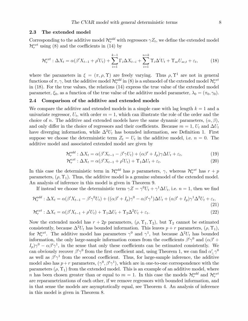
2.3 The extended model
Corresponding to the additive model Haddr with regressors γZt, we define the extended model
Hextr using (8) and the coeffi cients in (14) by
Hextr : ∆Xt = α(β′Xt−1 + ρ′Ut) +
k−1∑i=1
Γi∆Xt−i +
n+k∑i=1
Υi∆iUt + ΥseUse,t + εt, (18)
where the parameters in ξ = (π, ρ,Υ) are freely varying. Thus ρ,Υ1 are not in generalfunctions of π, γ, but the additive modelHadd
r in (8) is a submodel of the extended modelHextr
in (18). For the true values, the relations (14) express the true value of the extended modelparameter, ξ0, as a function of the true value of the additive model parameter, λ0 = (π0, γ0).
2.4 Comparison of the additive and extended models
We compare the additive and extended models in a simple case with lag length k = 1 and aunivariate regressor, Ut, with order m = 1, which can illustrate the role of the order and thechoice of n. The additive and extended models have the same dynamic parameters, (α, β),and only differ in the choice of regressors and their coeffi cients. Because m = 1, Ut and ∆Uthave diverging information, while ∆2Ut has bounded information, see Definition 1. Firstsuppose we choose the deterministic term Zt = Ut in the additive model, i.e. n = 0. Theadditive model and associated extended model are given by
Haddr : ∆Xt = α(β′Xt−1 − β′γUt) + (αβ′ + Ip)γ∆Ut + εt, (19)
Hextr : ∆Xt = α(β′Xt−1 + ρ′Ut) + Υ1∆Ut + εt. (20)
In this case the deterministic term in Haddr has p parameters, γ, whereas Hext
r has r + pparameters, (ρ,Υ1). Thus, the additive model is a genuine submodel of the extended model.An analysis of inference in this model is given in Theorem 9.If instead we choose the deterministic term γZ = γ0Ut + γ1∆Ut, i.e. n = 1, then we find
Haddr : ∆Xt = α(β′Xt−1 − β′γ0Ut) + ((αβ′ + Ip)γ
0 − αβ′γ1)∆Ut + (αβ′ + Ip)γ1∆2Ut + εt,
(21)
Hextr : ∆Xt = α(β′Xt−1 + ρ′Ut) + Υ1∆Ut + Υ2∆2Ut + εt. (22)
Now the extended model has r + 2p parameters, (ρ,Υ1,Υ2), but Υ2 cannot be estimatedconsistently, because ∆2Ut has bounded information. This leaves p+ r parameters, (ρ,Υ1),for Hext
r . The additive model has parameters γ0 and γ1, but because ∆2Ut has bounded
information, the only large-sample information comes from the coeffi cients β′γ0 and (αβ′ +Ip)γ
0 − αβ′γ1, in the sense that only these coeffi cients can be estimated consistently. Wecan obviously recover β′γ0 from the first coeffi cient and, using Theorem 1, we can find α′⊥γ
0
as well as β′γ1 from the second coeffi cient. Thus, for large-sample inference, the additivemodel also has p+ r parameters, (γ0, β′γ1), which are in one-to-one correspondence with theparameters (ρ,Υ1) from the extended model. This is an example of an additive model, wheren has been chosen greater than or equal to m = 1. In this case the models Hadd
r and Hextr
are reparametrizations of each other, if we remove regressors with bounded information, andin that sense the models are asymptotically equal, see Theorem 4. An analysis of inferencein this model is given in Theorem 8.
The CVAR model with general deterministic terms 9
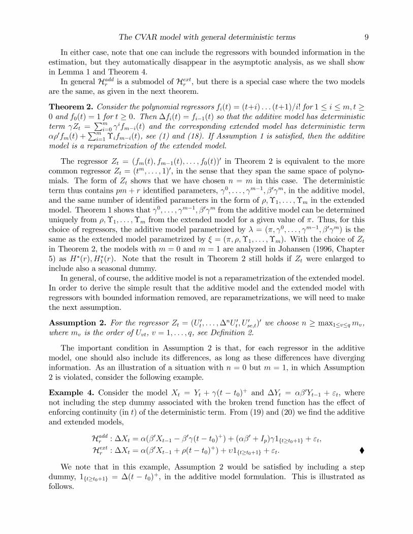
In either case, note that one can include the regressors with bounded information in theestimation, but they automatically disappear in the asymptotic analysis, as we shall showin Lemma 1 and Theorem 4.In general Hadd
r is a submodel of Hextr , but there is a special case where the two models
are the same, as given in the next theorem.
Theorem 2. Consider the polynomial regressors fi(t) = (t+i) . . . (t+1)/i! for 1 ≤ i ≤ m, t ≥0 and f0(t) = 1 for t ≥ 0. Then ∆fi(t) = fi−1(t) so that the additive model has deterministicterm γZt =
∑mi=0 γ
ifm−i(t) and the corresponding extended model has deterministic termαρ′fm(t) +
∑mi=1 Υifm−i(t), see (1) and (18). If Assumption 1 is satisfied, then the additive
model is a reparametrization of the extended model.
The regressor Zt = (fm(t), fm−1(t), . . . , f0(t))′ in Theorem 2 is equivalent to the morecommon regressor Zt = (tm, . . . , 1)′, in the sense that they span the same space of polyno-mials. The form of Zt shows that we have chosen n = m in this case. The deterministicterm thus contains pm+ r identified parameters, γ0, . . . , γm−1, β′γm, in the additive model,and the same number of identified parameters in the form of ρ,Υ1, . . . ,Υm in the extendedmodel. Theorem 1 shows that γ0, . . . , γm−1, β′γm from the additive model can be determineduniquely from ρ,Υ1, . . . ,Υm from the extended model for a given value of π. Thus, for thischoice of regressors, the additive model parametrized by λ = (π, γ0, . . . , γm−1, β′γm) is thesame as the extended model parametrized by ξ = (π, ρ,Υ1, . . . ,Υm). With the choice of Ztin Theorem 2, the models with m = 0 and m = 1 are analyzed in Johansen (1996, Chapter5) as H∗(r), H∗1 (r). Note that the result in Theorem 2 still holds if Zt were enlarged toinclude also a seasonal dummy.In general, of course, the additive model is not a reparametrization of the extended model.
In order to derive the simple result that the additive model and the extended model withregressors with bounded information removed, are reparametrizations, we will need to makethe next assumption.
Assumption 2. For the regressor Zt = (U ′t , . . . ,∆nU ′t , U
′se,t)
′ we choose n ≥ max1≤v≤qmv,where mv is the order of Uvt, v = 1, . . . , q, see Definition 2.
The important condition in Assumption 2 is that, for each regressor in the additivemodel, one should also include its differences, as long as these differences have diverginginformation. As an illustration of a situation with n = 0 but m = 1, in which Assumption2 is violated, consider the following example.
Example 4. Consider the model Xt = Yt + γ(t − t0)+ and ∆Yt = αβ′Yt−1 + εt, wherenot including the step dummy associated with the broken trend function has the effect ofenforcing continuity (in t) of the deterministic term. From (19) and (20) we find the additiveand extended models,
Haddr : ∆Xt = α(β′Xt−1 − β′γ(t− t0)+) + (αβ′ + Ip)γ1t≥t0+1 + εt,
Hextr : ∆Xt = α(β′Xt−1 + ρ(t− t0)+) + υ1t≥t0+1 + εt.
We note that in this example, Assumption 2 would be satisfied by including a stepdummy, 1t≥t0+1 = ∆(t − t0)+, in the additive model formulation. This is illustrated asfollows.
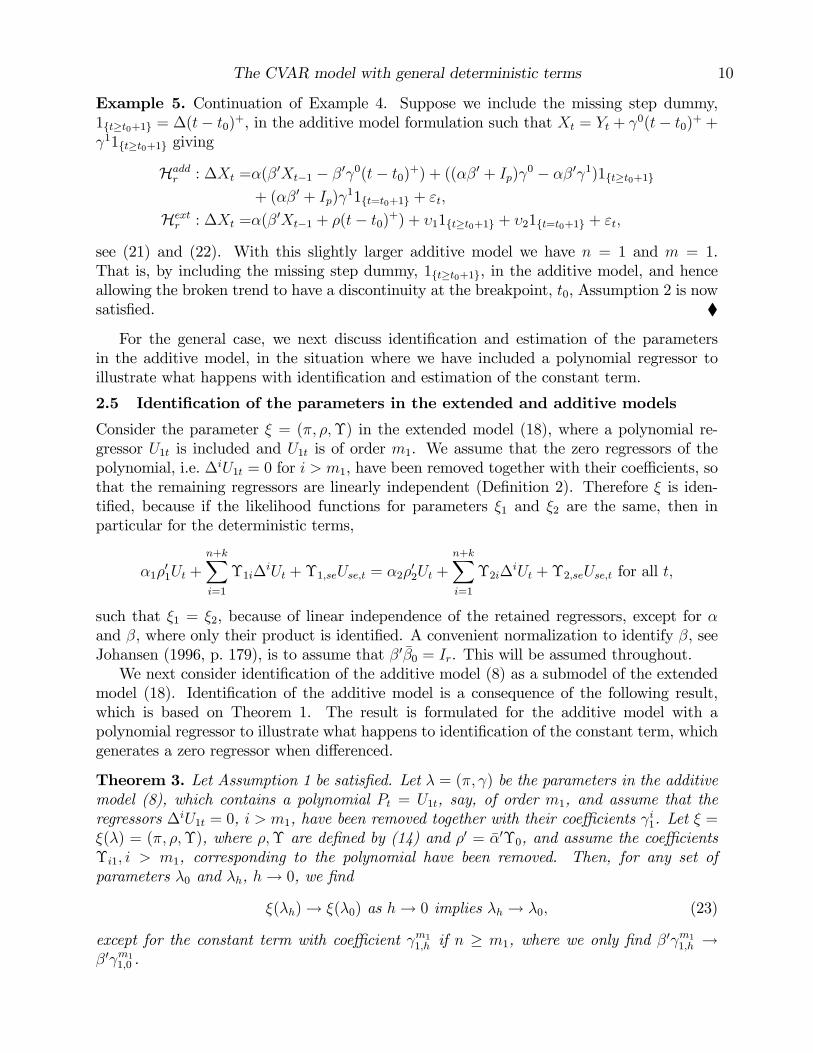
The CVAR model with general deterministic terms 10
Example 5. Continuation of Example 4. Suppose we include the missing step dummy,1t≥t0+1 = ∆(t− t0)+, in the additive model formulation such that Xt = Yt + γ0(t− t0)+ +γ11t≥t0+1 giving
Haddr : ∆Xt =α(β′Xt−1 − β′γ0(t− t0)+) + ((αβ′ + Ip)γ
0 − αβ′γ1)1t≥t0+1
+ (αβ′ + Ip)γ11t=t0+1 + εt,
Hextr : ∆Xt =α(β′Xt−1 + ρ(t− t0)+) + υ11t≥t0+1 + υ21t=t0+1 + εt,
see (21) and (22). With this slightly larger additive model we have n = 1 and m = 1.That is, by including the missing step dummy, 1t≥t0+1, in the additive model, and henceallowing the broken trend to have a discontinuity at the breakpoint, t0, Assumption 2 is nowsatisfied.
For the general case, we next discuss identification and estimation of the parametersin the additive model, in the situation where we have included a polynomial regressor toillustrate what happens with identification and estimation of the constant term.
2.5 Identification of the parameters in the extended and additive models
Consider the parameter ξ = (π, ρ,Υ) in the extended model (18), where a polynomial re-gressor U1t is included and U1t is of order m1. We assume that the zero regressors of thepolynomial, i.e. ∆iU1t = 0 for i > m1, have been removed together with their coeffi cients, sothat the remaining regressors are linearly independent (Definition 2). Therefore ξ is iden-tified, because if the likelihood functions for parameters ξ1 and ξ2 are the same, then inparticular for the deterministic terms,
α1ρ′1Ut +
n+k∑i=1
Υ1i∆iUt + Υ1,seUse,t = α2ρ
′2Ut +
n+k∑i=1
Υ2i∆iUt + Υ2,seUse,t for all t,
such that ξ1 = ξ2, because of linear independence of the retained regressors, except for αand β, where only their product is identified. A convenient normalization to identify β, seeJohansen (1996, p. 179), is to assume that β′β0 = Ir. This will be assumed throughout.We next consider identification of the additive model (8) as a submodel of the extended
model (18). Identification of the additive model is a consequence of the following result,which is based on Theorem 1. The result is formulated for the additive model with apolynomial regressor to illustrate what happens to identification of the constant term, whichgenerates a zero regressor when differenced.
Theorem 3. Let Assumption 1 be satisfied. Let λ = (π, γ) be the parameters in the additivemodel (8), which contains a polynomial Pt = U1t, say, of order m1, and assume that theregressors ∆iU1t = 0, i > m1, have been removed together with their coeffi cients γi1. Let ξ =ξ(λ) = (π, ρ,Υ), where ρ,Υ are defined by (14) and ρ′ = α′Υ0, and assume the coeffi cientsΥi1, i > m1, corresponding to the polynomial have been removed. Then, for any set ofparameters λ0 and λh, h→ 0, we find
ξ(λh)→ ξ(λ0) as h→ 0 implies λh → λ0, (23)
except for the constant term with coeffi cient γm11,h if n ≥ m1, where we only find β′γ
m11,h →
β′γm11,0 .
The CVAR model with general deterministic terms 11
Identification of the additive model as a submodel of the extended model follows fromTheorem 3 because if ξ(λ1) = ξ(λ0) then, choosing λh = λ1, we find from (23) that λ1 = λ0.Thus, a special case of Theorem 3 implies identification of the parameters of the additivemodel in the usual sense.However, in anticipation of our proof of consistency, Theorem 3 proves the more general
result that ξ depends continuously on the parameter λ, which one could call “continuousidentification”. The function ξ(λ) is clearly a continuous function of all parameters. If Λdenotes the parameter space for λ and we let ξ(Λ) denote the image of Λ, then Theorem 1shows that the function ξ restricted to ξ(Λ) is invertible. What is shown in Theorem 3 isthat this inverse function is continuous on ξ(Λ).The result in Theorem 3 thus shows continuous identification of γ, with the exception
that, if n ≥ m1 (so that the constant term, ∆m1Pt = ∆m1U1t, is included in the model), thenthe coeffi cient to the constant term is only identified in the β-directions.
2.6 Estimation of the parameters in the extended and additive models
For estimation we continue to assume that the zero regressors ∆iU1t = 0, i > m1, havebeen removed together with their coeffi cients, so that the remaining regressors are linearlyindependent. Then maximum likelihood estimation of the parameters of the extended model(18) can be conducted by reduced rank regression of ∆Xt on (X ′t−1, U
′t)′ corrected for the
non-zero regressors. See Anderson (1951) and Johansen (1996, Chapter 6).The additive model (8) has no simple closed-form estimation algorithm, but one can use a
numerical optimization algorithm to maximize the likelihood function, using that the modelis a submodel of the extended model subject to the restrictions (14). Starting values forthe iterations in the numerical optimization of the likelihood function can be found, usingTheorem 1, from parameter estimates of the extended model.
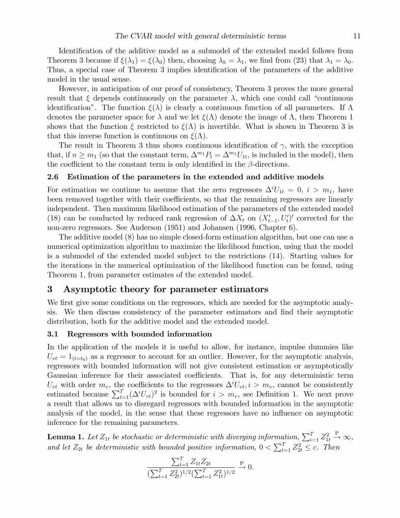
3 Asymptotic theory for parameter estimatorsWe first give some conditions on the regressors, which are needed for the asymptotic analy-sis. We then discuss consistency of the parameter estimators and find their asymptoticdistribution, both for the additive model and the extended model.
3.1 Regressors with bounded information
In the application of the models it is useful to allow, for instance, impulse dummies likeUvt = 1(t=t0) as a regressor to account for an outlier. However, for the asymptotic analysis,regressors with bounded information will not give consistent estimation or asymptoticallyGaussian inference for their associated coeffi cients. That is, for any deterministic termUvt with order mv, the coeffi cients to the regressors ∆iUvt, i > mv, cannot be consistentlyestimated because
∑Tt=1(∆iUvt)
2 is bounded for i > mv, see Definition 1. We next provea result that allows us to disregard regressors with bounded information in the asymptoticanalysis of the model, in the sense that these regressors have no influence on asymptoticinference for the remaining parameters.
Lemma 1. Let Z1t be stochastic or deterministic with diverging information,∑T
i=1 Z21t
P→∞,and let Z2t be deterministic with bounded positive information, 0 <
∑Tt=1 Z
22t ≤ c. Then∑T
t=1 Z1tZ2t
(∑T
t=1 Z22t)
1/2(∑T
t=1 Z21t)
1/2
P→ 0.
The CVAR model with general deterministic terms 12
A consequence of Lemma 1 is that the limit of the information matrix normalized by itsdiagonal elements will be asymptotically block diagonal, with one block corresponding toregressors with bounded information. This is used to prove that the latter type of regressorsdo not contribute to the asymptotic distribution of the remaining parameters. To this end,we now define the additive and extended models where regressors with bounded informationhave been removed, and subsequently we give the result.
Definition 3. Define Hadd∗r as the additive “core”model, given by Hadd
r in (8), but whereregressors with bounded information have been removed. Similarly define Hext∗
r as the ex-tended “core”model, given by Hext
r in (18), but where regressors with bounded informationhave been removed.
Theorem 4. The asymptotic distribution of the MLEs inHadd∗r is the same as the asymptotic
distribution of the MLEs of the same parameters in Haddr , and the asymptotic distribution
of the MLEs in Hext∗r is the same as the asymptotic distribution of the MLEs of the same
parameters in Hextr . Moreover, if Assumptions 1 and 2 are satisfied, then the models Hext∗
r
and Hadd∗r are reparametrizations of each other.
There are two important results in Theorem 4. First, the asymptotic distributions ofthe MLEs in the core models are the same as the asymptotic distributions of the MLEs ofthe same parameters in the models that include the regressors with bounded information.Consequently, we will therefore assume in the asymptotic analysis that all such regressorsand their coeffi cients have been removed. Second, under Assumptions 1 and 2, Theorem 4shows that the two core models, Hext∗
r and Hadd∗r , are reparametrizations of each other. That
is, in general Hextr and Hadd
r are not reparametrizations as for polynomials, see Theorem 2,but Assumption 2 is the important condition that allows us to establish that, asymptotically,a result that parallels Theorem 2 holds for the core models.
Example 6. Continuation of Examples 4 and 5. It is seen that the two models in Ex-ample 5 are not reparametrizations as for polynomials, see Theorem 2, but the coeffi cientυ2 is associated with a regressor with information
∑Tt=1 12
t=t0+1 = 1, and hence does notcontribute to the asymptotic analysis (Lemma 1). That is, by including the missing stepdummy, 1t≥t0+1, in the additive model, and hence allowing the broken trend to have adiscontinuity at the breakpoint, t0, Assumption 2 is now satisfied and the two models inExample 5 are asymptotically equivalent in the sense that their respective core models arereparametrizations of each other, see Theorem 4. 3.2 Partition and normalization of regressors with diverging information
In the following we consider only the core models,Hext∗r andHadd∗
r , based on the arguments inTheorem 4. That is, we remove regressors Uvt with bounded information and assume, withoutloss of generality, that all components Uvt have mv ≥ 0, and we discard the regressors ∆iUvtwith i > mv. We then find that the deterministic term in the extended model (18),
α
q∑v=1
ρ′vUvt +n+k∑i=1
q∑v=1
Υiv∆iUvt + ΥseUse,t, (24)
can be replaced– without changing the results of the asymptotic analysis– by
αρ′Z0t + Υ1Z1t, (25)

The CVAR model with general deterministic terms 13
where Z0t = Ut and Z1t are the regressors with diverging information including the seasonaldummies,
Z1t = (∆iUvt, 1 ≤ i ≤ minn+ k,mv, 1 ≤ v ≤ q;U ′se,t)′, (26)
and where the corresponding freely varying coeffi cients are
ρ′ = −β′γ0 and Υ1 = (Υiv, 1 ≤ i ≤ minn+ k,mv, 1 ≤ v ≤ q; Υse). (27)
We note that Z1t may be empty, in which case the remainder of the analysis is easily simplifiedaccordingly. We also note that the true values ρ0 and Υ1
0 are both functions of (π0, γ0), see(14).The asymptotic analysis is based on the behaviour of suitable product moments. We
therefore introduce the notation for product moments of sequences Ut, Vt,Wt, t = 1, . . . , T ,
〈U, V 〉T = T−1
T∑t=1
UtV′t ,
and for the residuals of Ut corrected for Wt,
(Ut|Wt) = Ut − 〈U,W 〉T 〈W,W 〉−1T Wt.
Product moments of residuals are denoted
〈U, V |W 〉T = 〈(U |W ), (V |W )〉T = 〈U, V 〉T − 〈U,W 〉T 〈W,W 〉−1T 〈W,V 〉T .
When the limit as T →∞ of a product moment exists, we use the notation 〈U, V 〉T → 〈U, V 〉.Next, for the asymptotic analysis we need the following normalizations of the regressors
and a mild condition to rule out asymptotically multicollinear regressors. For a regressorwith diverging information, i.e. ∆iUvt with i ≤ mv, we introduce the normalization MT iv.The normalizations of Z0t and Z1t are then given by the diagonal matrices
NT0 = diag(MT0v, 1 ≤ v ≤ q),
NT1 = diag(MT iv, 1 ≤ i ≤ mv, 1 ≤ v ≤ q; ι′s−1),
where ιs−1 is an (s− 1)-vector of ones, because the s− 1 seasonal dummies need no normal-ization. This defines the normalized regressors
Z0Tt = N−1T0Z0t and Z1Tt = N−1
T1Z1t. (28)
Assumption 3. The normalizations satisfy M−1T ivT
−1/2 → 0 and M−1T ivMT,i+1,v → 0 and the
asymptotic information matrix for the normalized regressors is nonsingular, i.e. satisfies⟨(Z0T
Z1T
),
(Z0T
Z1T
)⟩T
→⟨(
Z0
Z1
),
(Z0
Z1
)⟩> 0. (29)
Example 7. The nonsingularity condition in Assumption 3 rules out asymptotically multi-collinear regressors, and is easily satisfied in practice. As an example of what is ruled out,consider the regressor Ut = (t + 1t≥t0+1, t + 1t≥t0−1)
′ and suppose n = m = 1 such thatZ0t = Ut, Z1t = ∆Ut, see Definition 2 and (26). We normalize by MT0v = T and MT1v = 1
The CVAR model with general deterministic terms 14
and find Z0T [Tν] → (ν, ν)′ and Z1T [Tν] → (1, 1)′, such that the limit in (29) is singular. Inthis case, one could choose instead Ut = (t+ 1t≥t0+1, 1t≥t0−1− 1t≥t0+1)
′, which spans thesame space, but T−1U[Tν] → (ν, 0)′ and ∆U[Tν] → (1, 0)′, such that we can discard the secondcomponent and find Z0T [Tν] → ν, Z1T [Tν] → 1, which gives rise to consistent estimation witha non-singular asymptotic information matrix.
Finally, for a sequence εt, which is i.i.d. (0,Ω), we define the Brownian motion Wε as theweak limit of the partial sum of εt; that is, for St =
∑ti=1 εi we define Wε from
T−1/2S[Tν] = T−1/2
[Tν]∑t=1
εiD→ Wε(ν). (30)
Of course, Wε can be considered as Wε = Ω1/2B, where B is standard Brownian motion,but we find that using Wε is a simpler notation. For the asymptotic analysis we make thefollowing high-level assumption, for which primitive suffi cient conditions are well-known.
Assumption 4. The following limits as T →∞ exist and the convergences hold jointly,
T 1/2 〈ZjT , ε〉T = T−1/2N−1Tj
∑Tt=1 Zjtε
′t
D→ 〈Zj, ε〉 for j = 0, 1,
T−1/2 〈ZjT , St−1〉T = T−3/2N−1Tj
∑Tt=1 ZjtS
′t−1
D→ 〈Zj,Wε〉 for j = 0, 1,
T−1/2 〈St−1, ε〉T = T−3/2∑T
t=1 St−1ε′t
D→∫ 1
0Wε(dWε)
′ = 〈Wε, ε〉 .
Again, we use 〈Zj, ε〉, for example, as the notation for the limit of a product moment,because simple expressions in terms of stochastic integrals are not possible for all regressors.Examples of the limits in Assumption 4 are given next.
Example 8. Let Ut = (t, (t − t0)+)′ with ∆Ut = (1, 1t≥t0+1)′. Then MT0v = T and
MT1v = 1 and we note that M−1T ivT
−1/2 → 0 and M−1T0vMT1v → 0, reflecting that the order of
the regressor in this case decreases when differenced. We define
u(ν) = limT→∞
UT,[Tν] = limT→∞
N−1T0U[Tν] = (ν, (ν − ν0)+)′,
u(ν) = limT→∞
∆UT,[Tν] = limT→∞
N−1T1 ∆U[Tν] = (1, 1ν>ν0)
′.
For this example we find the limits, as T →∞,
〈UT ,∆UT 〉T = T−1∑T
t=1(T−1Ut)(∆Ut)′ →
∫ 1
0u(ν)u(ν)′dν = 〈U,∆U〉 ,
T 1/2 〈UT , ε〉T = T−1/2∑T
t=1 T−1Utε
′t
D→∫ 1
0u(ν)dWε(ν)′ = 〈U, ε〉 ,
T−1/2 〈UT , St−1〉T = T−3/2∑T
t=1 T−1UtS
′t−1
D→∫ 1
0u(ν)Wε(ν)′dν = 〈U,Wε〉 .
The previous example illustrates a relatively simple regressor, which when appropri-ately normalized has a limit, u(ν), in L2. In this case, the limit of the product momentT 1/2 〈UT , ε〉T , for example, can be expressed as a stochastic integral of u(ν) with respect toBrownian motion, Wε. However, such simple limit expressions are not always possible, asthe following example shows.
The CVAR model with general deterministic terms 15
Example 9. Let Use,t = (−1)t be a seasonal dummy variable. Then, as T →∞,
T 1/2 〈Use, ε〉T = T−1/2
T∑t=1
Use,tε′t
D→ N(0,Ω) = 〈Use, ε〉 ,
T−1/2 〈St−1, Use〉T = T−3/2
T∑t=1
St−1Use,t = OP (T−1),
where we note that 〈Use, ε〉 is not a stochastic integral involving a limit of Use,t because Use,tdoes not converge in L2.
3.3 Consistency of parameter estimators
Because we have eliminated regressors with bounded information by the above arguments,see in particular Theorem 4, from this point onwards the asymptotic analysis will focuson the additive and extended core models, Hadd∗
r and Hext∗r , see (8), 18), and Definition
3. The parameters of the additive core model, Hadd∗r , are given by λ = (π, γ) with true
value λ0 = (π0, γ0), and the parameters of the extended core model, Hext∗r , are given by
ξ = (π, ρ,Υ1) with true value ξ0 = (π0, ρ0,Υ10) = (π0,−β′0γ0,Υ
1(π0, γ0)).Let θ denote a parametrization of the conditional mean, e.g. λ or ξ. Then, for this
parametrization, the negative (quasi-) log-likelihood function is, apart from a constant term,
L(θ) = − logLT (θ,Ω = Ω0) =1
2trΩ−1
0
T∑t=1
εt(θ)εt(θ)′, (31)
where we have set Ω = Ω0 (without loss of generality for asymptotic inference on the remain-ing parameters) and εt(θ) are the residuals, which are defined for the additive and extended(core) models as
Hadd∗r : εt(λ) = ∆Xt − α(β′Xt−1 − β′γ0Z0t)−
k−1∑i=1
Γi∆Xt−i −Υ1(π, γ)Zt, (32)
Hext∗r : εt(ξ) = ∆Xt − α(β′Xt−1 + ρ′Z0t)−
k−1∑i=1
Γi∆Xt−i −Υ1Z1t, (33)
see (1) and (18). The MLEs of λ and ξ are then defined as λ = arg minλ L(λ) and ξ =arg minξ L(ξ), respectively. The latter can be obtained by reduced rank regression, but theformer requires numerical optimization, see Section 2.6.To prove consistency, we use the fact that both the additive and extended models can be
expressed as nonlinear submodels of a linear regression model. The Gaussian log-likelihoodfunction in the linear regression model is quadratic and therefore the level curves are ellipses.This means that, for any ellipse, the log-likelihood is smaller outside the ellipse than all valuesinside the ellipse. This simple fact can be used to prove consistency for a nonlinear submodel,as in the following result from Johansen (2006, Lemma 16, p. 114), which we will apply.
The CVAR model with general deterministic terms 16
Lemma 2. Consider the regression model yt = ς ′zt+εt, where εt is i.i.d. (0,Ω0), with stochas-tic or deterministic regressors, and let ς = ς(τ) be a continuously identified parametrizationof a submodel. We define the estimator τ as the minimizer of
trΩ−10
T∑t=1
(yt − ς(τ)′zt)(yt − ς(τ)′zt)′.
If the information diverges in probability for all components of zt, that is,
P(ωmin(
∑T
t=1ztz′t) > A
)→ 1 for all A > 0 as T →∞,
where ωmin(·) denotes the smallest eigenvalue of the argument, then τ exists with probabilityconverging to one and is consistent as T →∞.
Consistency of the continuously identified parameters in both the additive and extendedcore models thus follows from Theorems 3 and 4 because we only include regressors withdivergent information.
Theorem 5. Suppose Assumptions 1 and 3 are satisfied. In the extended core model Hext∗r ,
see Definition 3 and (18), with parameter ξ, the MLE ξ exists with probability converging to
one and ξ P→ ξ0. Similarly, in the additive core model Hadd∗r , see Definition 3 and (8), with
parameter λ, the MLE λ exists with probability converging to one and λ P→ λ0.
3.4 Asymptotic distribution of estimators
Letting Π0(L) denote the characteristic polynomial with the true values π0 inserted, we firstnote that the residuals (33) for the extended model are
εt(ξ) = Π(L)Xt − αρ′Z0t −Υ1Z1t = Π(L)Yt + Π(L)γ0Zt − αρ′Z0t −Υ1Z1t
= (Π(L)− Π0(L))Yt + Π(L)γ0Zt − αρ′Z0t −Υ1Z1t + εt. (34)
The deterministic term in (34) is
Π(L)γ0Zt − αρ′Z0t −Υ1Z1t = −α(β′γ00 + ρ′)Z0t − (Υ1 −Υ1(π, γ0))Z1t. (35)
The stochastic term in the residuals in (34) is, using the normalization β = β0 +β0⊥β′0⊥(β−
β0),
(Π(L)− Π0(L))Yt = −(α− α0)β′0Yt−1 − α(β − β0)′β0⊥β′0⊥Yt−1 −
k−1∑i=1
(Γi − Γi,0)∆Yt−i, (36)
see (2), where we note in particular that, from (4) and (30),
T−1/2β′0⊥Y[Tν] = T−1/2β′0⊥C0S[Tν] + oP (1)D→ β′0⊥C0Wε(ν)
as T →∞.We simplify the notation by defining new parameters to account for the parameters that
actually appear in (35) and (36) and to account for different normalizations. After deriving
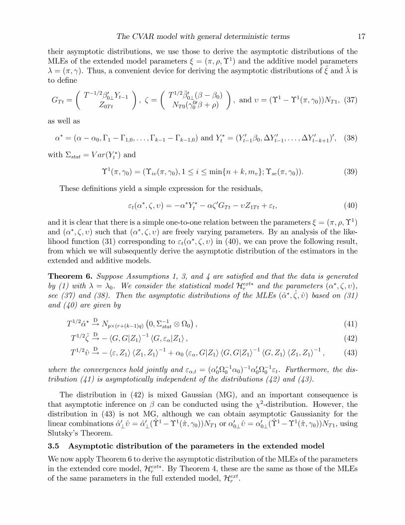
The CVAR model with general deterministic terms 17
their asymptotic distributions, we use those to derive the asymptotic distributions of theMLEs of the extended model parameters ξ = (π, ρ,Υ1) and the additive model parametersλ = (π, γ). Thus, a convenient device for deriving the asymptotic distributions of ξ and λ isto define
GTt =
(T−1/2β′0⊥Yt−1
Z0Tt
), ζ =
(T 1/2β′0⊥(β − β0)NT0(γ0′
0 β + ρ)
), and υ = (Υ1 −Υ1(π, γ0))NT1, (37)
as well as
α∗ = (α− α0,Γ1 − Γ1,0, . . . ,Γk−1 − Γk−1,0) and Y ∗t = (Y ′t−1β0,∆Y′t−1, . . . ,∆Y
′t−k+1)′, (38)
with Σstat = V ar(Y ∗t ) and
Υ1(π, γ0) = (Υiv(π, γ0), 1 ≤ i ≤ minn+ k,mv; Υse(π, γ0)). (39)
These definitions yield a simple expression for the residuals,
εt(α∗, ζ, υ) = −α∗Y ∗t − αζ ′GTt − υZ1Tt + εt, (40)
and it is clear that there is a simple one-to-one relation between the parameters ξ = (π, ρ,Υ1)and (α∗, ζ, υ) such that (α∗, ζ, υ) are freely varying parameters. By an analysis of the like-lihood function (31) corresponding to εt(α∗, ζ, υ) in (40), we can prove the following result,from which we will subsequently derive the asymptotic distribution of the estimators in theextended and additive models.
Theorem 6. Suppose Assumptions 1, 3, and 4 are satisfied and that the data is generatedby (1) with λ = λ0. We consider the statistical model Hext∗
r and the parameters (α∗, ζ, υ),see (37) and (38). Then the asymptotic distributions of the MLEs (α∗, ζ, υ) based on (31)and (40) are given by
T 1/2α∗D→ Np×(r+(k−1)q)
(0,Σ−1
stat ⊗ Ω0
), (41)
T 1/2ζD→ −〈G,G|Z1〉−1 〈G, εα|Z1〉 , (42)
T 1/2υD→ −〈ε, Z1〉 〈Z1, Z1〉−1 + α0 〈εα, G|Z1〉 〈G,G|Z1〉−1 〈G,Z1〉 〈Z1, Z1〉−1 , (43)
where the convergences hold jointly and εα,t = (α′0Ω−10 α0)−1α′0Ω−1
0 εt. Furthermore, the dis-tribution (41) is asymptotically independent of the distributions (42) and (43).
The distribution in (42) is mixed Gaussian (MG), and an important consequence isthat asymptotic inference on β can be conducted using the χ2-distribution. However, thedistribution in (43) is not MG, although we can obtain asymptotic Gaussianity for thelinear combinations α′⊥υ = α′⊥(Υ1−Υ1(π, γ0))NT1 or α′0⊥υ = α′0⊥(Υ1−Υ1(π, γ0))NT1, usingSlutsky’s Theorem.
3.5 Asymptotic distribution of the parameters in the extended model
We now apply Theorem 6 to derive the asymptotic distribution of the MLEs of the parametersin the extended core model, Hext∗
r . By Theorem 4, these are the same as those of the MLEsof the same parameters in the full extended model, Hext
r .
The CVAR model with general deterministic terms 18
Theorem 7. Suppose Assumptions 1, 3, and 4 are satisfied and that the data is generated by(1) with λ = λ0. We consider the statistical model Hext∗
r and the parameters ξ = (π, ρ,Υ1).Then:
(i) The asymptotic distribution of T 1/2(α−α0, Γ1−Γ1,0, . . . , Γk−1−Γk−1,0) is given in (41)in Theorem 6, and the asymptotic distribution of T β′0⊥(β − β0) follows from (42).
(ii) For ρ′ = (ρ′1, . . . , ρ′q), ζ = (ζ ′1, ζ
′2)′ defined in (37), ζ ′2 = (ζ2,1, . . . , ζ2,q), and 1 ≤ v ≤ q,
the expansions
ρ′v − ρ′v0 = −(β − β0)′γ00v − β′(γ0
v − γ00v) = −(T 1/2ζ ′1β
′0⊥γ
00v)T
−1 + (T 1/2ζ2,v)M−1T0vT
−1/2
(44)shows that the asymptotic distribution of ρ−ρ0, suitably normalized, follows from (42),and is mixed Gaussian.
(iii) For 1 ≤ v ≤ q and 1 ≤ i ≤ mv, the asymptotic distribution of Υiv − Υiv,0 = Υiv −Υiv(π0, γ0) consists of two terms,
Υiv −Υiv,0 = (T 1/2υiv)T−1/2M−1
T iv + (T 1/2Υiv(π − π0, γ0))T−1/2, (45)
see (37). The asymptotic distribution of T 1/2υiv is given in (43), and, replacing β byβ0, the asymptotic distribution of T 1/2Υiv(π−π0, γ0) depends only on that of α∗, whichis Gaussian and given in (41), and the two terms on the right-hand side of (45) areasymptotically independent.
The asymptotic distributions in parts (ii) and (iii) of Theorem 7 both depend only onthe largest term. That is, in part (ii) the asymptotic distribution depends on the relationbetween the normalizations T−1 andM−1
T0vT−1/2 as well as the value of the parameter β′0⊥γ
00v,
whereas in part (iii) it depends on the relation between T−1/2M−1T iv and T
−1/2. Haldrup (1996)encounters a similar problem of different limit behaviour of estimators in the context of aDickey-Fuller regression with a slope coeffi cient.
3.6 Asymptotic distribution of the estimators in the additive model
Under Assumption 2, the extended and additive core models are reparametrizations of eachother, see Theorem 4. Thus, in this case we have that Υ1 = Υ1(π, γ), such that
Υ1(π, γ)−Υ1(π, γ0) = Υ1(π, γ − γ0). (46)
We use this fact, together with the simple one-to-one relation between the parameters inthe extended core model, ξ, and the parameters in Theorem 6, and the one-to-one relationbetween ξ and λ(ξ) in Theorem 1 to derive the asymptotic distribution of the maximumlikelihood estimator for the additive model, which we here denote λ = λ(ξ), from the resultsin Theorem 6.
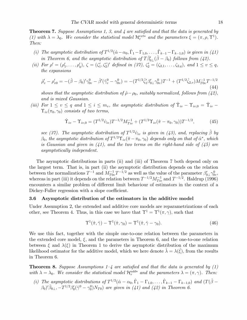
Theorem 8. Suppose Assumptions 1—4 are satisfied and that the data is generated by (1)with λ = λ0. We consider the statistical model Hadd∗
r and the parameters λ = (π, γ). Then:
(i) The asymptotic distributions of T 1/2(α − α0, Γ1 − Γ1,0, . . . , Γk−1 − Γk−1,0) and (T (β −β0)′β0⊥,−T 1/2β′0(γ0 − γ0
0)NT0) are given in (41) and (42) in Theorem 6.
The CVAR model with general deterministic terms 19
(ii) For 1 ≤ v ≤ q and 0 ≤ i ≤ mv, the asymptotic distributions of T 1/2MT iv(γiv − γi0v) are
given in terms of those of υiv = (Υiv −Υiv(π, γ0))MT iv, see (37) and (43), as follows,
T 1/2β′0(γiv − γiv0)MT iv = −T 1/2α′0υiv + oP (1), 1 ≤ i ≤ mv, (47)
T 1/2α′0⊥Γ0(γiv − γiv0)MT,i+1,v = T 1/2α′0⊥υi+1,v + oP (1), 0 ≤ i ≤ mv − 1, (48)
T 1/2 vec(γse − γse0 ) = (k∑i=0
M i′s ⊗ Φi0)−1T 1/2 vec(υse). (49)
(iii) The distributions (47)—(49) are asymptotically independent of the distribution (41)given above.
The main result in Theorem 8 is that the simple condition in Assumption 2 of includingenough differenced regressors in the additive model, implies that the additive and extendedcore models are reparametrizations of each other (Theorem 4). This permits relativelystraightforward inference on the parameters of the additive model. Moreover, by Theorem4, the asymptotic distributions of the MLEs of the parameters in the additive core model,Hadd∗r , given in Theorem 8, are the same as those for the same parameters in the full additive
model, Haddr .
Recall that the distribution in (42) is mixed Gaussian (MG), so that asymptotic inferenceon β can be conducted using the χ2-distribution also in the additive model. Also note thatT 1/2α′0⊥υi+1,v is asymptotically Gaussian, see (43), but T 1/2α′0υiv is neither asymptoticallyGaussian nor mixed Gaussian. Thus, to use Theorem 8, for example, to test hypotheseson the parameter γ0
v , the parameter needs to be divided into two components for which theestimators have different convergence rates as in (42) and (48). This is discussed in detailin Section 4.
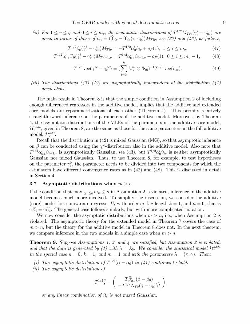
3.7 Asymptotic distributions when m > n
If the condition that max1≤v≤qmv ≤ n in Assumption 2 is violated, inference in the additivemodel becomes much more involved. To simplify the discussion, we consider the additive(core) model for a univariate regressor Ut with order m, lag length k = 1, and n = 0, that isγZt = γUt. The general case follows similarly, but with more complicated notation.We now consider the asymptotic distributions when m > n, i.e., when Assumption 2 is
violated. The asymptotic theory for the extended model in Theorem 7 covers the case ofm > n, but the theory for the additive model in Theorem 8 does not. In the next theorem,we compare inference in the two models in a simple case when m > n.
Theorem 9. Suppose Assumptions 1, 3, and 4 are satisfied, but Assumption 2 is violated,and that the data is generated by (1) with λ = λ0. We consider the statistical model Hadd∗
r
in the special case n = 0, k = 1, and m = 1 and with the parameters λ = (π, γ). Then:
(i) The asymptotic distribution of T 1/2(α− α0) in (41) continues to hold.(ii) The asymptotic distribution of
T 1/2ζ =
(T β′0⊥(β − β0)
−T 1/2NT0(γ − γ0)′β
),
or any linear combination of it, is not mixed Gaussian.
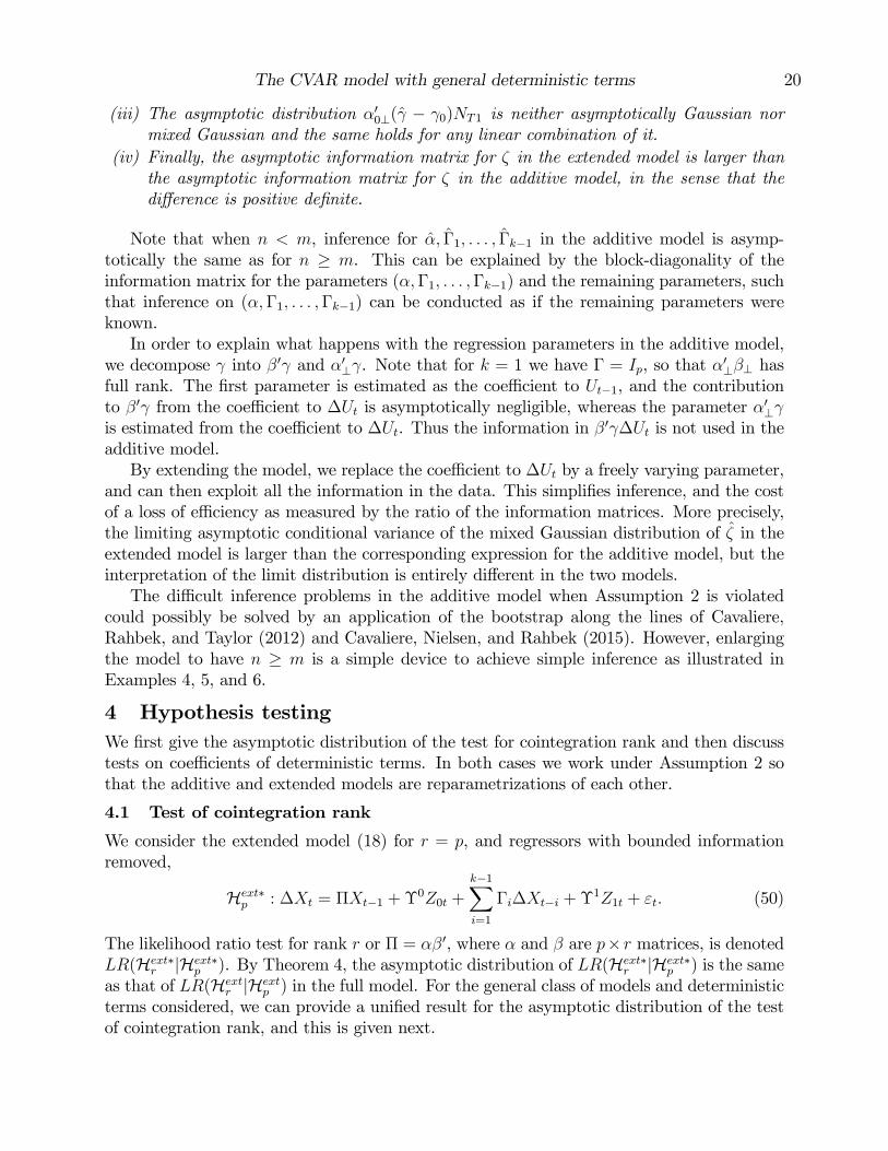
The CVAR model with general deterministic terms 20
(iii) The asymptotic distribution α′0⊥(γ − γ0)NT1 is neither asymptotically Gaussian normixed Gaussian and the same holds for any linear combination of it.
(iv) Finally, the asymptotic information matrix for ζ in the extended model is larger thanthe asymptotic information matrix for ζ in the additive model, in the sense that thedifference is positive definite.
Note that when n < m, inference for α, Γ1, . . . , Γk−1 in the additive model is asymp-totically the same as for n ≥ m. This can be explained by the block-diagonality of theinformation matrix for the parameters (α,Γ1, . . . ,Γk−1) and the remaining parameters, suchthat inference on (α,Γ1, . . . ,Γk−1) can be conducted as if the remaining parameters wereknown.In order to explain what happens with the regression parameters in the additive model,
we decompose γ into β′γ and α′⊥γ. Note that for k = 1 we have Γ = Ip, so that α′⊥β⊥ hasfull rank. The first parameter is estimated as the coeffi cient to Ut−1, and the contributionto β′γ from the coeffi cient to ∆Ut is asymptotically negligible, whereas the parameter α′⊥γis estimated from the coeffi cient to ∆Ut. Thus the information in β′γ∆Ut is not used in theadditive model.By extending the model, we replace the coeffi cient to ∆Ut by a freely varying parameter,
and can then exploit all the information in the data. This simplifies inference, and the costof a loss of effi ciency as measured by the ratio of the information matrices. More precisely,the limiting asymptotic conditional variance of the mixed Gaussian distribution of ζ in theextended model is larger than the corresponding expression for the additive model, but theinterpretation of the limit distribution is entirely different in the two models.The diffi cult inference problems in the additive model when Assumption 2 is violated
could possibly be solved by an application of the bootstrap along the lines of Cavaliere,Rahbek, and Taylor (2012) and Cavaliere, Nielsen, and Rahbek (2015). However, enlargingthe model to have n ≥ m is a simple device to achieve simple inference as illustrated inExamples 4, 5, and 6.
4 Hypothesis testingWe first give the asymptotic distribution of the test for cointegration rank and then discusstests on coeffi cients of deterministic terms. In both cases we work under Assumption 2 sothat the additive and extended models are reparametrizations of each other.
4.1 Test of cointegration rank
We consider the extended model (18) for r = p, and regressors with bounded informationremoved,
Hext∗p : ∆Xt = ΠXt−1 + Υ0Z0t +
k−1∑i=1
Γi∆Xt−i + Υ1Z1t + εt. (50)
The likelihood ratio test for rank r or Π = αβ′, where α and β are p× r matrices, is denotedLR(Hext∗
r |Hext∗p ). By Theorem 4, the asymptotic distribution of LR(Hext∗
r |Hext∗p ) is the same
as that of LR(Hextr |Hext
p ) in the full model. For the general class of models and deterministicterms considered, we can provide a unified result for the asymptotic distribution of the testof cointegration rank, and this is given next.
The CVAR model with general deterministic terms 21
Theorem 10. Under Assumptions 1— 4, the asymptotic distribution of the test of cointe-grating rank in either the extended core model, Hext∗
r , or in the additive core model, Hadd∗r ,
is given by
−2 logLR(Hext∗r |Hext∗
p )D→ tr〈εα⊥ , G|Z1〉 〈G,G|Z1〉−1 〈G, εα⊥|Z1〉,
where εα⊥,t = (α′0⊥Ω0α0⊥)−1/2α′0⊥εt is i.i.d. (0, Ip−r). By Theorem 4, the statistics LR(Hextr |Hext
p )and LR(Hadd
r |Haddp ) have the same asymptotic distribution as LR(Hext∗
r |Hext∗p ).
Note that the limit distribution of the rank test depends on the type of regressors andneeds to be simulated for the various cases. However, it does not depend on the values ofthe regression parameters, i.e. the rank test is asymptotically similar with respect to theregression parameters, see Nielsen and Rahbek (2000). This is a consequence of startingfrom the additive formulation with n ≥ max1≤v≤qmv, and deriving the extended model fromthe additive model. In the innovation formulation (6), this is not the case, see for examplethe analysis of the model with an unrestricted constant term in Johansen (1996, Chapter13.5).
4.2 Tests of hypotheses on deterministic terms
We consider inference on the coeffi cients γiv, 0 ≤ i ≤ mv ≤ n, in the additive model underAssumption 2. It follows from Theorems 6 and 8 that the limit distribution of γiv − γiv0
naturally decomposes in two parts, and we therefore split the hypothesis γiv = 0 into a testthat β′γiv = 0 and a test that α′⊥Γγiv = 0 assuming β′γiv = 0 (since the matrix (β,Γ′α⊥) hasfull rank under Assumption 1, see Theorem 1). It appears natural first to investigate if γ0
v ,i.e. the coeffi cient of Uvt, is zero. If we cannot reject that it is zero, then we can proceed totest that the coeffi cient of ∆Uvt is zero, that is, test the hypothesis γ1
v = 0, assuming γ0v = 0,
etc. Thus we can apply the asymptotic distributions in Theorems 7 and 8 as in Theorem 11to test recursively that γiv = 0, provided we assume that γjv = 0, 0 ≤ j < i.Under Assumption 2 the additive and extended core models are reparametrizations (The-
orem 4). Therefore, estimation of the unrestricted model can be performed by reduced rankregression of ∆Xt on (X ′t−1, Z
′0t)′ corrected for lagged ∆Xt and the regressors Z1t, where
Z0t = Ut, see (25) and Section 2.6. Under the hypothesis β′γ0v = 0, the parameters can be
estimated in the same way by reduced rank regression, but removing Uvt from Z0t. Finally,if both β′γ0
v = 0 and α′⊥Γγ0v = 0, so that γ0
v = 0, the estimation can also be performed byreduced rank regression, but replacing Uvt with ∆Uvt in Z0t and removing ∆Uvt from Z1t.
Theorem 11. Let Assumptions 1—4 be satisfied. Then:
(i) In the additive core model, Hadd∗r , the likelihood ratio test for the hypothesis ρ′v =
−β′γ0v = 0 is asymptotically χ2(r)-distributed.
(ii) In the additive core model, Hadd∗r , with mv ≥ 1, the likelihood ratio test for the hypoth-
esis α′⊥Γγ0v = 0, given that ρ′v = 0, is asymptotically χ2(p− r)-distributed.
(iii) In the additive core model, Hadd∗r , with mv ≥ 1, the likelihood ratio test for the joint
hypothesis, γ0v = 0, is asymptotically χ2(p)-distributed.
(iv) By Theorem 4, the same results hold in the additive model, Haddr .
The CVAR model with general deterministic terms 22
5 ConclusionsWe define the CVAR model with additive deterministic terms and derive the correspondinginnovation formulation which is nonlinear in the parameters. This additive model is extendedto a model which is linear in the coeffi cients of the deterministic terms and hence allowsestimation by reduced rank regression. A general class of regressors is defined and for eachregressor its order. This setup allows a discussion of the relation between the innovationformulation of the additive model and its extension.A simple condition for when the additive and the extended model are (asymptotically)
identical is given. The condition, given as Assumption 2, is that for each regressor in theadditive model one should also include its differences, as long as they have diverging infor-mation. If this recommendation is not followed, asymptotic inference is considerably morecomplicated. For example, when the regressor is a polynomial or power function, say ta forsome a > −1/2, the recommendation is to include (at least) m = [a + 1/2] differences ofta, which seems like a natural thing to do. Indeed, not doing so seems quite strange in mostcircumstances. On the other hand, for the broken trend function, (t− t0)+, it may in fact bereasonable to exclude the first difference, 1t≥t0+1, when insisting on continuity of the trendfunction as in Example 4. However, the recommendation is to include the first differenceanyway, even if it is believed to be zero, because including it leads to simple inference, seeExamples 5 and 6.We derive the asymptotic distribution of the rank test in both the additive and the
extended models, and show that both are similar with respect to the regression parameters.The asymptotic distribution of the parameter estimates is found to be a mixture of a Gaussiandistribution and a mixed Gaussian distribution, and finally we show how it can be appliedto test that the regression coeffi cients are zero.
A Appendix: proofs of resultsA.1 Proof of Theorem 1
The two results in (15) follow from (14) when multiplying by α′ and α′⊥, respectively, usingΦ0 = −αβ′ and Φ1 = αβ′ + Γ. It follows from
(β,Γ′α⊥)′(β, β⊥) =
(β′β 0α′⊥Γβ α′⊥Γβ⊥
), (51)
and Assumption 1 that α′⊥Γβ⊥ has full rank, and hence that also (β,Γ′α⊥) has full rank,so that the relations in (15) can be solved for γi. To solve for γse, we let (ωj, vj), j =1, . . . , s − 1, be the eigenvalues and eigenvectors of Ms. It is clear from (14) that Υse isa linear function of γse, and we want to show that this function is non-singular, that is,that Υse =
∑ki=0 Φiγ
seM is = 0 implies γse = 0. To see this, post-multiply by vj and use
M isvj = ωijvj, such that
0 = Υsevj =k∑i=0
ΦiγseM i
svj =
k∑i=0
Φiωijγ
sevj = Π(1− ωj)γsevj.
Now ωj = 1 − e2πij/s, j = 1, . . . , s − 1, see Example 3, such that Π(1 − ωj) = Π(e2πij/s),which by Assumption 1 has full rank, such that γsevj = 0 for all j and hence γse = 0. The
The CVAR model with general deterministic terms 23
definition of Υse is therefore
vec(Υse) = (k∑i=0
M is ⊗ Φi) vec(γse),
where∑k
i=0Mis ⊗ Φi is of full rank. The solution is then given by (16).
A.2 Proof of Theorem 2
The result ∆fi(t) = fi−1(t) follows from the identity
(t+ i) · · · (t+ 1)− (t− 1 + i) · · · t = (t+ i) ((t− 1 + i) · · · (t+ 1))− ((t− 1 + i) · · · (t+ 1)) t
= ((t− 1 + i) · · · (t+ 1)) (t+ i− t) = ((t− 1 + i) · · · (t+ 1)) i
after division by i!.The additive formulation of model (1) with Zt = (fm(t), . . . , f0(t))′ has n = m and
deterministic term
Π(L)γZt =k∑i=0
Φi∆i
m∑j=0
γjfm−j(t) =k∑i=0
m∑j=0
Φiγjfm−j−i(t)
=m∑s=0
Υsfm−s(t) = αρ′fm(t) +m∑s=1
Υsfm−s(t),
where the penultimate equality follows because ∆jfm(t) = 0 for j > m.
A.3 Proof of Theorem 3
The proof follows from Theorem 1 because ξ(λ) determines λ as a linear, and hence contin-uous, function except for α′⊥Γγm1
1 (in the case n ≥ m1).
A.4 Proof of Lemma 1
For T1 ≤ T , we decompose the numerator asT∑t=1
Z1tZ2t =
T1∑t=1
Z1tZ2t +T∑
t=T1+1
Z1tZ2t,
and evaluate the second term using the Cauchy-Schwarz inequality,
|T∑
t=T1+1
Z1tZ2t| ≤ (
T∑t=T1+1
Z21t)
1/2(
T∑t=T1+1
Z22t)
1/2 ≤ (
T∑t=1
Z21t)
1/2(
∞∑t=T1+1
Z22t)
1/2.
Because∑T
t=1 Z22t ≤ c, it follows that, for all ε > 0 and T1 suffi ciently large, we have
|T∑
t=T1+1
Z1tZ2t|(T∑t=1
Z21t)−1/2 ≤ (
∞∑t=T1+1
Z22t)
1/2 ≤ ε/2.
Finally, because∑T
t=1 Z21t
P→ ∞, we can choose T so large that, for any (fixed) T1 and anyδ > 0, we have
|T1∑t=1
Z1tZ2t|(T∑t=1
Z21t)−1/2 ≤ ε/2
with probability greater than 1− δ, which completes the proof.
The CVAR model with general deterministic terms 24
A.5 Proof of Theorem 4
Lemma 1 shows that, for both the additive and the extended models, the limit of the infor-mation matrix normalized by its diagonal elements is asymptotically block diagonal. Oneblock corresponds to the coeffi cients of the regressors with bounded information and anothercorresponds to the parameters in the core model. This implies that the asymptotic distrib-utions of the MLEs in the core models are the same as the asymptotic distributions of theMLEs of the same parameters in the full models.Under Assumptions 1 and 2, the core models, Hext∗
r and Hadd∗r , have the same number of
parameters. For the core model Hext∗r , see (27) the parameters are, apart from π and Υse,
the rq +∑q
v=1mv parameters collected in
(ρ,Υi1, . . . ,Υi,mv , 1 ≤ v ≤ q). (52)
For the core model Hadd∗r , the parameters are, see (11), apart from π and Υse, the pq +∑q
i=1(p(mv − 1) + r) parameters collected in
(γ0, γ1v , . . . , γ
mv−1v , β′γmv
v , 1 ≤ v ≤ q). (53)
Theorem 1 shows how (52) can be recovered from (53) and vice versa. Thus, the core modelsare reparametrizations of each other.
A.6 Proof of Theorem 5
We can express both the additive model (8) and the extended model (18) as nonlinearsubmodels of a linear regression model as follows. Because we have normalized β on β′β0 =Ir, we can define θ = β′0⊥(β−β0) such that β = β0 +β0⊥θ. Then the extended model (18) is
∆Xt = αβ′0Xt−1 + αθ′β′0⊥Xt−1 + αρ0′Z0t +k−1∑i=1
Γi∆Xt−i + Υ1Z1t + Υ2Z2t + εt,
which is a submodel of the linear regression model
∆Xt = α(β′0Xt−1) + φ(β′0⊥Xt−1) + ψZ0t +k−1∑i=1
Γi∆Xt−i + Υ1Z1t + Υ2Z2t + εt (54)
defined by the restrictions φ = αθ′, ψ = αρ0′, and the remaining parameters being the samein the two models. From Theorem 3 it follows that, because α0ρ
0′h → α0ρ
0′0 and α0θ
′h → α0θ
′0
implies θh → θ0 and ρ0h → ρ0
0, the extended model is continuously identified in the largerlinear regression model (54). Similarly, the additive model is continuously identified in theextended model and hence in the larger linear regression model. The result now followsimmediately from Theorems 3 and 4.
A.7 Proof of Theorem 6
The likelihood is given in (31) with εt(θ) replaced by the residuals εt(α∗, ζ, υ), see 40).Derivatives of εt: At the true values, (α∗, ζ, υ) = (α∗0, ζ0, υ0) = (0, 0, 0), we find the
derivatives
Dα∗εt(α∗0, ζ0, υ0; dα∗) = −(dα∗)Y ∗t ,
Dζεt(α∗0, ζ0, υ0; dζ) = −α0(dζ)′GTt,
Dυεt(α∗0, ζ0, υ0; dυ) = −(dυ)Z1Tt.
The CVAR model with general deterministic terms 25
Score and information: We denote the score function with respect to α∗, for example,in the direction dα∗ as Sα∗ = Dα∗ logL(α∗0, ζ0, υ0; dα∗). The information with respect to α∗
and ζ, for example, is similarly denoted by Iα∗ζ = D2α∗ζ logL(α∗0, ζ0, υ0; dα∗, dζ). Then the
scores are
T−1/2Sα∗ = − trΩ−10 (dα∗)T 1/2 〈Y ∗, ε〉T
D→ − trΩ−10 (dα∗) 〈Y ∗, ε〉, (55)
T−1/2Sζ = − trΩ−10 α0(dζ)′T 1/2 〈GT , ε〉T
D→ − trΩ−10 α0(dζ)′ 〈G, ε〉, (56)
T−1/2Sυ = − trΩ−10 (dυ)T 1/2 〈Z1T , ε〉T
D→ − trΩ−10 (dυ) 〈Z1, ε〉, (57)
and the diagonal elements of the information are
T−1Iα∗α∗ = trΩ−10 (dα∗) 〈Y ∗, Y ∗〉T (dα∗)′+ oP (1)
P→ trΩ−10 (dα∗)Σstat(dα
∗)′, (58)
T−1Iζζ = trΩ−10 α0(dζ)′ 〈GT , GT 〉T (dζ)α′0+ oP (1)
D→ trΩ−10 α0(dζ)′ 〈G,G〉 (dζ)α′0, (59)
T−1Iυυ = trΩ−10 (dυ) 〈Z1T , Z1T 〉T (dυ)′+ oP (1)
D→ trΩ−10 (dυ) 〈Z1, Z1〉 (dυ)′.
There is one non-zero off-diagonal element,
T−1Iζυ = trΩ−10 α0(dζ)′ 〈GT , Z1T 〉T (dυ)′+ oP (1)
D→ trΩ−10 α0(dζ)′ 〈G,Z1〉 (dυ)′,
and the following are asymptotically negligible,
T−1Iα∗ζ = trΩ−10 (dα∗) 〈Y ∗, GT 〉T (dζ)α′0+ oP (1)
P→ 0, (60)
T−1Iα∗υ = trΩ−10 (dα∗) 〈Y ∗, Z1T 〉T (dυ)′+ oP (1)
P→ 0.
Because the information is asymptotically block diagonal, α∗ and (ζ , υ) are asymptoticallyindependent, and we consider inference separately for α∗ and (ζ, υ).The asymptotic distribution of T 1/2α∗: By the usual Taylor expansion of the likelihood
equations, we find that the equation for the asymptotic distribution of T 1/2α∗ is given by
trΩ−10 (dα∗) 〈Y ∗, Y ∗〉T (T 1/2α∗)′ = − trΩ−1
0 (dα∗)T 1/2 〈Y ∗, ε〉T+ oP (1) for all dα∗,
and henceΣstatT
1/2α∗′ = −T 1/2 〈Y ∗, ε〉T + oP (1),
which by the Central Limit Theorem gives the result in (41).The asymptotic distribution of T 1/2(ζ , υ): Similarly, we find the equations for determining
the limit distribution of (ζ , υ),
〈GT , GT 〉T (T 1/2ζ)α′0Ω−10 α0 + 〈GT , Z1T 〉T (T 1/2υ)′Ω−1
0 α0 = −T 1/2 〈GT , ε〉T Ω−10 α0 + oP (1),
(61)
〈Z1T , GT 〉T (T 1/2ζ)α′0Ω−10 + 〈Z1T , Z1T 〉T (T 1/2υ)′Ω−1
0 = −T 1/2 〈Z1T , ε〉T Ω−10 + oP (1).
(62)
Pre-multiplying (62) by 〈GT , Z1T 〉T 〈Z1T , Z1T 〉−1T , post-multiplying by α0, and subtracting
the result from (61) we find
〈GT , GT |Z1T 〉T (T 1/2ζ)α′0Ω−10 α0 = −〈GT , ε|Z1T 〉T Ω−1
0 α0,
which implies (42) and inserted into (62) gives (43).
The CVAR model with general deterministic terms 26
A.8 Proof of Theorem 7
First note that Hext∗r with the parameters ξ is a simple one-to-one reparametrization of Hext∗
r
with the parameters (α∗, ζ, υ). Thus, these parametrizations have the same likelihood andthe MLEs of ξ can easily be found from those of (α∗, ζ, υ) and vice versa.Proof of (i): The result for the dynamic parameters π = (α, β,Γ1, . . . ,Γk−1) follows
directly from (41) and (42) by the definitions of α∗ and ζ, see (37) and (38).Proof of (ii): Using ρ′v = −β′γ0
v and the definition of ζ = (ζ ′1, ζ′2)′ in (37), we find the
expansion (44). This expansion shows that the limit is a linear combination of the elementsof the limit of ζ, and hence mixed Gaussian, see (42).Proof of (iii): The expansion (45) follows directly from the definition of υiv in (37).
Clearly the limit of the first term, T 1/2υiv, is given in (43). Because β converges at rate T(super consistency), see (42), we can replace β by β0 in the second term, T 1/2Υiv(π−π0, γ0),without changing the asymptotic properties. Hence, T 1/2Υiv(π − π0, γ0) becomes a linearcombination of T 1/2α∗, see (38), and is therefore asymptotically Gaussian. Asymptoticindependence of the two terms follows because the limits in (42) and (43) are independent,see Theorem 6.
A.9 Proof of Theorem 8
Under Assumption 2, the extended and additive core models are reparametrizations of eachother, see Theorem 4. Moreover, the simple one-to-one relation between the parameters inthe extended core model, ξ, and the parameters in Theorem 6 then show that in fact theadditive core model and the extended core model parametrized by (α∗, ζ, υ) are reparame-trizations. Hence, they have the same likelihood and the MLEs of the parameters of theadditive model can be found directly from the MLEs in Theorem 6 using Theorem 1.Proof of (i): First, β′0(γ0 − γ0
0)NT0 = β′(γ0 − γ00)NT0 + oP (1) by Slutsky’s Theorem and
consistency of β. Under Assumption 2 it follows from Theorem 4 that β′(γ0 − γ00)NT0 =
−(ρ′ + β′γ00)NT0 = ζ ′2, where ζ = (ζ ′1, ζ
′2)′, see (37). The results for the dynamic parameters
π = (α, β,Γ1, . . . ,Γk−1) and for β′0(γ0 − γ00)NT0 then follow directly from (41) and (42) by
the definitions of α∗ and ζ, see (37) and (38).Proof of (ii): Again, by Slutsky’s Theorem and consistency of β it follows that T 1/2β′0(γiv−
γiv0)MT iv = T 1/2β′(γiv − γiv0)MT iv + oP (1) and T 1/2α′0⊥Γ0(γiv − γiv0)MT,i+1,v = T 1/2α′⊥Γ(γiv −γiv0)MT,i+1,v + oP (1). Next, we note that, under Assumption 2, υiv = (Υiv − Υiv(π, γ0)) =Υiv(π, γ − γ0) by (46) and Theorem 4. By Theorem 1, applied to (π, γ0) and (π, γ), we thenfind that β′(γiv − γiv0) for i = 1, . . . ,mv and α′⊥Γ(γiv − γiv0) for i = 0, . . . ,mv − 1 can beexpressed in terms of υiv as
T 1/2β′(γiv − γiv0)MT iv = −T 1/2α′0Υiv(π, γ − γ0)MT iv + T 1/2α′ mini,k∑j=1
Φj(γi−jv − γi−jv0 )MT iv
= −T 1/2α′Υiv(π, γ − γ0)MT iv + oP (1)
= −T 1/2α′υiv + oP (1) = −T 1/2α′0υiv + oP (1)
using that M−1T,i−j,vMT iv → 0 for j = 1, . . . ,mini, k (by Assumption 3) and using Slutsky’s
The CVAR model with general deterministic terms 27
Theorem again for the final equality. Similarly, for i = 0, . . . ,mv − 1,
T 1/2α′⊥Γ(γiv − γiv0)MT,i+1,v =T 1/2α′⊥Υi+1,v(π, γ − γ0)MT,i+1,v
− T 1/2α′⊥
mini+1,k∑j=2
Φj(γi+1−jv − γi+1−j
v0 )MT,i+1,v
=T 1/2α′⊥Υi+1,v(π, γ − γ0)MT,i+1,v + oP (1)
=T 1/2α′⊥υi+1,v + oP (1) = T 1/2α′0⊥υi+1,v + oP (1)
because M−1T,i−j+1,vMT,i+1,v → 0 for j = 2, . . . ,mini + 1, k,mv. This proves (47) and (48).
Finally, (49) follows directly from vectorization of (14) and noting that∑k
i=0 Mi′s ⊗ Φ0i is
invertible by Theorem 3.Proof of (iii): That (47)—(49) are asymptotically independent of (41), is shown in Theo-
rem (6).
A.10 Proof of Theorem 9
Proof of (i): Because k = 1 and n = 0 we have Ut = Zt, γ0 = γ, and
εt(λ) = ∆Xt − α(β′Xt−1 − β′γZt−1)− γ∆Zt.
Furthermore, α′0⊥Γ0β0⊥ = α′0⊥β0⊥ and γ − γ0 can be decomposed as
γ − γ0 = α(β′α)−1β′(γ − γ0) + β⊥(α′⊥β⊥)−1α′⊥(γ − γ0). (63)
We define ζ ′2 = −β′(γ − γ0)MT0 and φ′ = T 1/2(α′⊥β⊥)−1α′⊥(γ − γ0)MT1 as well as α∗ =α− α0, Y
∗t = β′0Yt−1, see (37) and (38). The corresponding likelihood is then based on
εt(α∗, ζ, φ) = −α∗Y ∗t − αζ ′GTt − α(β′α)−1ζ ′2M
−1T0MT1Z1Tt − β⊥φ′Z1Tt + εt,
see (40). We note that ζ2 appears in two places, but M−1T0MT1 → 0, and therefore the term
ζ ′2M−1T0MT1Z1Tt disappears in the asymptotic analysis of the score and information, because
it is dominated by the term αζ ′GTt.Mimicking the analysis in the proof of Theorem 6, we find at the true values, α∗0 = 0, ζ0 =
0, φ0 = 0, the derivatives
Dα∗εt(α∗0, ζ0, φ0; dα∗) = −(dα∗)Y ∗t ,
Dζεt(α∗0, ζ0, φ0; dζ) = −α0(dζ)′GTt − α0(β′0α0)−1(dζ2)′M−1
T0MT1Z1Tt = −α0(dζ)′GTt + o(1),
Dφεt(α∗0, ζ0, φ0; dφ) = −β0⊥(dφ)′Z1Tt.
The limits of the scores for α∗ and ζ are therefore given in (55) and (56), and for φ we find
T−1/2Sφ = − trΩ−10 β0⊥(dφ)′T 1/2 〈Z1T , ε〉T
D→ − trΩ−10 β0⊥(dφ)′ 〈Z1, ε〉.
The limits of the information matrix blocks Iα∗α∗, Iζζ , and Iα∗ζ are given in (58), (59), and(60), respectively, and for φ we find
T−1Iφφ = trΩ−10 β0⊥(dφ)′ 〈Z1T , Z1T 〉T (dφ)β′0⊥+ oP (1)
D→ trΩ−10 β0⊥(dφ)′ 〈Z1, Z1〉 (dφ)β′0⊥,
T−1Iα∗φ = trΩ−10 (dα∗) 〈Y ∗, Z1T 〉T (dφ)β′0⊥+ oP (1)
P→ 0,
T−1Iζφ = trΩ−10 α0(dζ)′ 〈GT , Z1T 〉T (dφ)β′0⊥+ oP (1)
D→ trΩ−10 α0(dζ)′ 〈G,Z1〉 (dφ)β′0⊥.
The CVAR model with general deterministic terms 28
Thus, the only difference compared with the extended model is the factor β0⊥, which comesfrom estimating φ = (α′0⊥β0⊥)−1α′0⊥(γ − γ0) as the coeffi cient to ∆Zt. It is seen that thelimit information is block-diagonal corresponding to α∗ and (ζ, φ), such that the asymptoticdistribution of T 1/2α∗ = T 1/2(α− α0) is as given in (41) in Theorem 6.Proof of (ii): We find the equations for determining the limit distribution of the MLE
T 1/2(ζ , φ), but compared with (61) and (62) there is now an extra factor β0⊥ in (65),
〈G,G〉 (T 1/2ζ)α′0Ω−10 α0 + 〈G,Z1〉 (T 1/2φ)β′0⊥Ω−1
0 α0D→− 〈G, ε〉Ω−1
0 α0, (64)
〈Z1, G〉 (T 1/2ζ)α′0Ω−10 β0⊥ + 〈Z1, Z1〉 (T 1/2φ)β′0⊥Ω−1
0 β0⊥D→− 〈Z1, ε〉Ω−1
0 β0⊥. (65)
Eliminating T 1/2φ from (64), we find the right-hand side
−〈G, ε〉Ω−10 α0 + 〈G,Z1〉 〈Z1, Z1〉−1 〈Z1, ε〉Ω−1
0 β0⊥(β′0⊥Ω−10 β0⊥)−1β′0⊥Ω−1
0 α0.
If we condition on G, or equivalently on α′0⊥Wε, the right-hand side is Gaussian with meanproportional to
E(〈Z1, ε〉Ω−10 β0⊥|α′0⊥Wε) = 〈Z1, ε〉α0⊥(α′0⊥Ω0α0⊥)−1α′0⊥β0⊥ 6= 0. (66)
Thus, the limit distribution of T 1/2ζ is not mixed Gaussian, and the same holds for anylinear combination of T 1/2ζ.Proof of (iii): If we eliminate T 1/2ζ from the equations (64) and (65), we find that the
right-hand side becomes
〈Z1, G〉 〈G,G〉−1 〈G, ε〉Ω−10 α0(α′0Ω−1
0 α0)−1α′0Ω−10 β0⊥ − 〈Z1, ε〉Ω−1
0 β0⊥.
Conditional on G this distribution has mean −E(〈Z1, ε〉Ω−10 β0⊥|α′0⊥Wε), see (66), and the
limit distribution of T 1/2φ is neither Gaussian nor mixed Gaussian, and the same holds forany linear combination.Proof of (iv): From (61) and (62) we find the equations to determine the limit distribution
of the MLE in the extended model T 1/2(ζ , υ),
〈G,G〉 (T 1/2ζ)α′0Ω−10 α0 + 〈G,Z1〉 (T 1/2υ)Ω−1
0 α0D→− 〈G, ε〉Ω−1
0 α0,
〈Z1, G〉 (T 1/2ζ)α′0Ω−10 + 〈Z1, Z1〉 (T 1/2υ)Ω−1
0D→− 〈Z1, ε〉Ω−1
0 ,
and from these we find that the limit of the information matrix for (ζ, υ) in the extendedmodel is, (
α′0Ω−10 α0 ⊗ 〈G,G〉 Ω−1
0 α0 ⊗ 〈G,Z1〉α′0Ω−1
0 ⊗ 〈Z1, G〉 Ω−10 ⊗ 〈Z1, Z1〉
)=
(Iextζζ Iextζυ
Iextυζ Iextυυ
),
say. In the additive model, the limit of the information matrix for (ζ, φ) is, see (64) and(65), (
α′0Ω−10 α0 ⊗ 〈G,G〉 α′0Ω−1
0 β0⊥ ⊗ 〈G,Z1〉β′0⊥Ω−1
0 α0 ⊗ 〈Z1, G〉 β′0⊥Ω−10 β0⊥ ⊗ 〈Z1, Z1〉
)=
(Iaddζζ Iaddζφ
Iaddφζ Iaddφφ
).
We note that the left factors in the information matrix for (ζ, φ) satisfy the relation
α′0Ω−10 α0 − α′0Ω−1
0 β0⊥(β′0⊥Ω−10 β0⊥)−1β′0⊥Ω−1
0 α0 = α′0β0(β′0Ω−10 β0)−1β′0α0 > 0.
The CVAR model with general deterministic terms 29
This has the consequence that
Iaddζζ − Iaddζφ (Iaddφφ )−1Iaddφζ
= α′0Ω−10 α0 ⊗ 〈G,G〉 − α′0Ω−1
0 β0⊥(β′0⊥Ω−10 β0⊥)−1β′0⊥Ω−1
0 α0 ⊗ 〈G,Z1〉 〈Z1, Z1〉−1 〈Z1, G〉> α′0Ω−1
0 α0 ⊗ 〈G,G〉 − α′0Ω−10 α0 ⊗ 〈G,Z1〉 〈Z1, Z1〉−1 〈Z1, G〉
= α′0Ω−10 α0 ⊗ 〈G,G|∆Z〉 = Iextζζ − Iextζυ (Iextυυ )−1Iextυζ ,
where the inequality means that the difference is positive definite, almost surely. It followsthat the asymptotic conditional variance of ζ in the additive model is larger than that of ζin the extended model because
AsV ar(ζadd) = (Iaddζζ − Iaddζφ (Iaddφφ )−1Iaddφζ )−1 < (Iextζζ − Iextζυ (Iextυυ )−1Iextυζ )−1 = AsV ar(ζext),
almost surely.
A.11 Proof of Theorem 10
Normalization of parameters and an auxiliary model : We introduce the p × r matrix β0 ofrank r, decompose Π as
Π = Πβ0β′0 + Πβ0⊥β
′0⊥,
and define the auxiliary hypothesis
H = Πβ0⊥ = 0 and β′0(γ0 − γ00) = 0.
We note that under the assumptions in H, Π = αβ′0 for α = Πβ0, such that
H = Π = αβ′0 and β′0(γ0 − γ0
0) = 0.
Thus, if β∗ = (β′, β′γ0)′ then
Hext∗p ∩H = Hext∗
r ∩ β∗ = β∗0.
To facilitate the analysis of the test for rank, we introduce the extra hypothesis H inmodels Hext∗
p and Hext∗r , see Lawley (1956) for an early application of this idea or Johansen
(2002, p. 1947) and Johansen and Nielsen (2012, p. 2699) for applications to the (fractional)CVAR model. We then find
LR(Hext∗r |Hext∗
p ) =maxHext∗r
LT (ξ)
maxHext∗pLT (ξ)
=maxHext∗p ∩H LT (ξ)
maxHext∗pLT (ξ)
/maxHext∗r ∩β∗=β∗0 LT (ξ)
maxHext∗rLT (ξ)
.
That is, instead of the rank test statistic, we analyze the ratio of two test statistics,
LR(Hext∗r |Hext∗
p ) =LR(H|Hext∗
p )
LR(β∗ = β∗0 |Hext∗r )
. (67)
Analysis of LR(H|Hext∗p ): We apply the formulas (35) and (36) for Hext∗
p , using α−α0 =(Π− Π0)β0, to find
−Π(L)(γ − γ0)Zt = Π(γ0 − γ00)NT0Z0Tt −Υ1(π, γ − γ0)NT1Z1Tt,
(Π(L)− Π0(L))Yt = −α∗Y ∗t − T 1/2Πβ0⊥T−1/2β′0⊥Yt−1,
The CVAR model with general deterministic terms 30
where α∗ and Y ∗t are given in (38). Defining
ζ ′ = (T 1/2Πβ0⊥,Π(γ0 − γ00)NT0) and GTt =
(T−1/2β′0⊥Yt−1
Z0Tt
), (68)
we then obtain the residuals
εt(ξ) = −α∗Y ∗t − ζ ′GTt −Υ1(π, γ − γ0)NT1Z1Tt + εt,
see also (40). This shows that the likelihood for Hext∗p is maximized by regression of εt on
(GTt, Y∗t , Z1Tt), and the maximized likelihood function becomes
−2T−1 logLmax(Hext∗p ) = log det 〈ε, ε|GT , Y
∗, Z1T 〉T = log det 〈ε, ε|GT , Z1T 〉T + oP (1)
because 〈ε, Y ∗〉T = OP (T−1/2). The hypothesis H is just ζ = 0, and we find similarly
−2T−1 logLmax(Hext∗p ∩H) = log det 〈ε, ε|Y ∗, Z1T 〉T = log det 〈ε, ε|Z1T 〉T + oP (1).
It follows from
〈ε, ε|GT , Z1T 〉T = 〈ε, ε|Z1T 〉T − 〈ε,GT |Z1T 〉T 〈GT , GT |Z1T 〉−1T 〈GT , ε|Z1T 〉T
and 〈ε, ε|Z1T 〉TP→ Ω0 that
−2 logLR(H|Hext∗p ) = trΩ−1
0 T 1/2 〈ε,GT |Z1T 〉T 〈GT , GT |Z1T 〉−1T T 1/2 〈GT , ε|Z1T 〉T+ oP (1)
D→ trΩ−10 〈ε,G|Z1〉 〈G,G|Z1〉−1 〈G, ε|Z1〉. (69)
Analysis of LR(β∗ = β∗0 |Hext∗r ): The hypothesis we want to test here involves only β
and γ0, and because inference on α∗ is asymptotically independent of inference on (β, γ0),we can assume that α∗ = α∗0 = 0 for the asymptotic analysis of this statistic. We now findfor β = β0 + β0⊥β
′0⊥(β − β0) that
−Π(L)|α∗=α∗0(γ − γ0)Zt = α0β′(γ0 − γ0
0)NT0Z0Tt −Υ1(π, γ − γ0)NT1Z1Tt,
(Π(L)− Π0(L))|α∗=α∗0Yt = −α0(β − β0)′β0⊥β′0⊥Yt−1.
We define GTt as above, see (68), and define
ζ ′ = (T 1/2(β − β0)′β0⊥, β′(γ0 − γ0
0)NT0),
and note that the hypothesis β = β0 and β′γ0 = β′0γ00 is again ζ = 0. We then find
Hext∗r : εt(ξ) = −α0ζ
′GTt −Υ1(π, γ − γ0)NT1Z1Tt + εt.
We split the residuals by multiplying by α′Ω0 = (α′0Ω−10 α0)′α′0Ω−1
0 and α′0⊥ into
α′Ω0εt(ξ) = −ζ ′GTt − α′Ω0Υ1(π, γ − γ0)NT1Z1Tt + α′Ω0εt,
α′0⊥εt(ξ) = −α′0⊥Υ1(π, γ − γ0)NT1Z1Tt + α′0⊥εt.
The CVAR model with general deterministic terms 31
The errors α′Ω0εt and α′0⊥εt are independent and both sets of residuals are analyzed byregression, and we find
−2T−1 logLmax(Hext∗r ) = log det
⟨α′Ω0ε, α
′Ω0ε|GT , Z1T
⟩T
+ log det 〈α′0⊥ε, α′0⊥ε|Z1T 〉Tand
−2T−1 logLmax(Hext∗r ∩ ζ = 0) = log det
⟨α′Ω0ε, α
′Ω0ε|Z1T
⟩T
+ log det 〈α′0⊥ε, α′0⊥ε|Z1T 〉T .
The test of β∗ = β∗0 in Hext∗r , using
⟨α′Ω0ε, α
′Ω0ε⟩−1
T
P→ α′Ω0Ω0αΩ0 = (α′0Ω−10 α0)−1, is
−2 logLR(β∗ = β∗0 |Hext∗r )
= trα′0Ω−10 α0T
1/2⟨α′Ω0ε,GT |Z1T
⟩T〈GT , GT |Z1T 〉−1
T T 1/2⟨GT , α
′Ω0ε|Z1T
⟩T+ oP (1)
D→ trΩ−10 α0(α′0Ω−1
0 α0)−1α′0Ω−10 〈ε,G|Z1〉 〈G,G|Z1〉−1 〈G, ε|Z1〉. (70)
Analysis of LR(Hext∗r |Hext∗
p ): By (67), the test for rank r converges to the differencebetween (69) and (70), i.e.,
−2 logLR(Hext∗r |Hext∗
p )D→ tr(Ω−1
0 −Ω−10 α0(α′0Ω−1
0 α0)−1α′0Ω−10 ) 〈ε,G|Z1〉 〈G,G|Z1〉−1 〈G, ε|Z1〉.
Using the identity Ω−10 − Ω−1
0 α0(α′0Ω−10 α0)−1α′0Ω−1
0 = α0⊥(α′0⊥Ω0α0⊥)−1α′0⊥ and definingεα⊥,t = (α′0⊥Ω0α0⊥)−1/2α′0⊥εt, we obtain the result.
A.12 Proof of Theorem 11
Proof of (i): We find from Theorem 7(ii) that ρ′v − ρ′v0, suitably normalized, is mixedGaussian. Hence, the likelihood ratio test for β′γ0
v = −ρ′v = 0 is a χ2(r) test.Proof of (ii): We test the hypothesis that α′⊥Γγ0
v = 0 using the statistic α′⊥Γγ0v , assuming
that β′0γ0v0 = −ρ′v0 = 0. Under the null that also α′0⊥Γ0γ
0v0 = 0, we find that γ0
v0 = 0 because(β0,Γ
′0α0⊥) has full rank by Assumption 1, and it follows that α′⊥Γγ0
v = α′⊥Γ(γ0v−γ0
0v). FromSlutsky’s Theorem and consistency of π (Theorem 5), we then find
T 1/2α′⊥Γ(γ0v − γ0
v0)MT1v = T 1/2α′0⊥Γ0(γ0v − γ0
v0)MT1v + oP (1).
The asymptotic distribution of the first term on the right-hand side is found from (48) inTheorem 8 and (43) in Theorem 6,
T 1/2α′0⊥Γ0(γ0v − γ0
v0)MT1v = T 1/2α′0⊥υ1v + oP (1)D→ −α′0⊥ 〈ε, Z1〉 〈Z1, Z1〉−1A
for a suitable selection matrix A. This limit is Gaussian so that T 1/2α′⊥Γ(γ0v − γ0
v0)MT1v isasymptotically Gaussian, and hence the likelihood ratio test for α′⊥Γγ0
v = 0 is asymptoticallyχ2(p− r).Proof of (iii): Follows trivially from (i) and (ii).
AcknowledgementsWe are grateful to two anonymous referees, Giusepppe Cavaliere, Anders Rahbek, and sem-inar participants at various universities and conferences for comments, and to Bent Nielsenfor help. We would like to thank the Canada Research Chairs program, the Social Sciencesand Humanities Research Council of Canada (SSHRC), and the Center for Research inEconometric Analysis of Time Series (CREATES - DNRF78, funded by the Danish NationalResearch Foundation) for research support.
The CVAR model with general deterministic terms 32
References1. Anderson, T.W. (1951). Estimating linear restrictions on regression coeffi cients formultivariate normal distributions. Annals of Mathematical Statistics 22, pp. 327—351.
2. Belke, A., and Beckmann, J. (2015). Monetary policy and stock prices —cross-countryevidence from cointegrated VAR models. Journal of Banking and Finance 54, pp.254—265.
3. Cavaliere, G., Nielsen, H.B., and Rahbek, A. (2015). Bootstrap testing of hypotheseson cointegration relations in VAR models. Econometrica 83, pp. 813—831.
4. Cavaliere, G., Rahbek, A., and Taylor, A.M.R. (2012). Bootstrap determination of thecointegration rank in VAR models. Econometrica 80, pp. 1721—1740.
5. Doornik, J.A., Hendry, D.F., and Nielsen, B. (1998). Inference in cointegrated models:UK M1 revisited. Journal of Economic Surveys 12, pp. 533—572.
6. Haldrup, N. (1996). Mirror image distributions and the Dickey-Fuller regression witha maintained trend. Journal of Econometrics 72, pp. 301—312.
7. Hendry, D.F., and Juselius, K. (2001). Explaining cointegration analysis: part II.Energy Journal 22, pp. 75—120.
8. Johansen, S. (1996). Likelihood-Based Inference in Cointegrated Vector AutoregressiveModels (2.ed.), Oxford University Press, Oxford.
9. Johansen, S. (2002). A small sample correction for the test of cointegrating rank inthe vector autoregressive model. Econometrica 70, pp. 1929—1961.
10. Johansen, S. (2006). Statistical analysis of hypotheses on the cointegrating relationsin the I(2) model. Journal of Econometrics 132, pp. 81—115.
11. Johansen, S., Mosconi, R., and Nielsen, B. (2000). Cointegration analysis in the pres-ence of structural breaks in the deterministic trend. Econometrics Journal 3, pp.216—249.
12. Johansen, S. and Nielsen, M.Ø. (2012). Likelihood inference for a fractionally cointe-grated vector autoregressive model. Econometrica 80, pp. 2667—2732.
13. Juselius, K. (2006). The Cointegrated VAR Model: Methodology and Applications,Oxford University Press, Oxford.
14. Juselius, K. (2009). The long swings puzzle: what the data tell when allowed to speakfreely. In T. Mills and K. Patterson (eds.) Palgrave Handbook of Econometrics, Volume2: Applied Econometrics, Palgrave-MacMillan, New York, pp. 349—384.
15. Lütkepohl, H., and Saikkonen, P. (2000). Testing for the cointegrating rank of a VARprocess with a time trend. Journal of Econometrics 95, pp. 177—198.
16. Miller, K.S. (1968). Linear Difference Equations, Benjamin, New York.17. Nielsen, H.B. (2004). Cointegration analysis in the presence of outliers. Econometrics
Journal 7, pp. 249—271.18. Nielsen, H.B. (2007). UK money demand 1873-2011: a long time series analysis and
event study. Cliometrics 1, pp. 45—61.19. Nielsen, B., and Rahbek, A. (2000). Similarity issues in cointegration analysis. Oxford
Bulletin of Economics and Statistics 62, pp. 5—22.20. Pretis, F. (2015). Econometric models of climate systems: the equivalence of two-
component energy balance models and cointegrated VARs. Department of Economics
The CVAR model with general deterministic terms 33
Discussion Paper Series 750, University of Oxford.21. Pretis, F., Schneider, L., Smerdon, J.E., and Hendry, D.F. (2016). Detecting volcanic
eruptions in temperature reconstructions by designed break-indicator saturation. Jour-nal of Economic Surveys 30, pp. 403—429.
22. Rahbek, A., and Mosconi, R. (1999). Cointegration rank inference with stationaryregressors in VAR models. Econometrics Journal 2, pp. 76—91.
23. Saikkonen, P., and Lütkepohl, H. (2000a). Testing for the cointegrating rank of a VARprocess with an intercept. Econometric Theory 16, pp. 373—406.
24. Saikkonen, P., and Lütkepohl, H. (2000b). Testing for the cointegrating rank of aVAR process with structural shifts. Journal of Business & Economic Statistics 18,pp. 451—464.
25. Trenkler, C., Saikkonen, P., and Lütkepohl, H. (2007). Testing for the cointegratingrank of a VAR process with a level shift and a trend break. Journal of Time SeriesAnalysis 29, pp. 331—358.
Top Related