


Languages
Pages
Legal

ARTICLE IN PRESS
JID: FINEC [m3Gdc; September 6, 2018;2:41 ]
Journal of Financial Economics 0 0 0 (2018) 1–30
Contents lists available at ScienceDirect
Journal of Financial Economics
journal homepage: www.elsevier.com/locate/jfec
The CAPM strikes back? An equilibrium model with disasters
�
Hang Bai a , Kewei Hou
b , c , Howard Kung
d , e , Erica X.N. Li f , Lu Zhang
b , g , ∗
a School of Business, University of Connecticut, 2100 Hillside Road, Storrs, CT 06269, USA b Fisher College of Business, Ohio State University, 2100 Neil Avenue, Columbus OH 43210, USA c China Academy of Financial Research (CAFR), China d London Business School, Regent’s Park, Sussex Place, London NW1 4SA, UK e The Center for Economic and Policy Research (CEPR), USA f Cheung Kong Graduate School of Business, 1 East Chang An Avenue, Oriental Plaza, Beijing 100738, China g National Bureau of Economic Research (NBER), USA
a r t i c l e i n f o
Article history:
Received 12 May 2015
Revised 12 February 2018
Accepted 23 February 2018
Available online xxx
JEL classification:
G12
G14
Keywords:
CAPM
Rare disasters
Measurement errors
Consumption CAPM
General equilibrium
a b s t r a c t
Embedding disasters into a general equilibrium model with heterogeneous firms induces
strong nonlinearity in the pricing kernel, helping explain the empirical failure of the (con-
sumption) CAPM. Our single -factor model reproduces the failure of the CAPM in explaining
the value premium in finite samples without disasters and its relative success in sam-
ples with disasters. Due to beta measurement errors, the estimated beta-return relation
is flat, consistent with the beta “anomaly,” even though the true beta-return relation is
strongly positive. Finally, the consumption CAPM fails in simulations, even though a non-
linear model with the true pricing kernel holds exactly by construction.
Published by Elsevier B.V.
� For helpful comments, we thank our discussants Michael Brennan,
Max Croce, and Francisco Gomes, as well as Ron Balvers, Jack Favilukis,
Wayne Ferson, Finn Kydland, Ian Martin, Thien Nguyen, Bill Schwert
(the editor), Berk Sensoy, René Stulz, Selale Tuzel, Mike Weisbach, In-
grid Werner, Chen Xue, and other seminar participants at Federal Reserve
Bank of New York, McMaster University, Ohio State University, Peking
University, the 2013 Society of Economic Dynamics Annual Meetings, the
2013 University of British Columbia Summer Finance Conference, the 2014
American Economic Association Annual Meetings, the 2014 Econometric
Society Winter Meetings, the 2015 University of Southern California Mar-
shall Ph.D. Conference in Finance, and the 2016 Society of Financial Stud-
ies Cavalcade. We are particularly indebted to John Cochrane (the referee)
for extensive and insightful comments that have improved greatly the
quality of our work. This paper supersedes our previous work on “The
CAPM strikes back? An investment model with disasters.”∗ Corresponding author at: Fisher College of Business, Ohio State Uni-
versity, 2100 Neil Avenue, Columbus OH 43210, USA.
E-mail addresses: [email protected] (H. Bai), [email protected]
(K. Hou), [email protected] (H. Kung), [email protected] (E.X.N. Li),
[email protected] (L. Zhang).
https://doi.org/10.1016/j.jfineco.2018.08.009
0304-405X/Published by Elsevier B.V.
Please cite this article as: H. Bai et al., The CAPM strikes back?
Economics (2018), https://doi.org/10.1016/j.jfineco.2018.08.009
1. Introduction
Despite similar market betas, firms with high book-
to-market (value firms) earn higher average stock returns
than firms with low book-to-market (growth firms). This
stylized fact is commonly referred to as the value premium
puzzle. In the US sample from July 1963 to June 2017, the
high-minus-low book-to-market decile return is, on aver-
age, 0.47% per month ( t = 2 . 53 ). However, its market beta
is only 0.07 ( t = 0 . 86 ), giving rise to an economically large
alpha of 0.43% ( t = 1 . 89 ) in the capital asset pricing model
(CAPM) ( Fama and French, 1992 ). However, the CAPM per-
forms better in explaining the value premium in the long
sample from July 1926 onward that contains the Great De-
pression ( Ang and Chen, 2007 ). The high-minus-low re-
turn is, on average, 0.48% ( t = 2 . 5 ), but its CAPM alpha
An equilibrium model with disasters, Journal of Financial

2 H. Bai et al. / Journal of Financial Economics 0 0 0 (2018) 1–30
ARTICLE IN PRESS
JID: FINEC [m3Gdc; September 6, 2018;2:41 ]
is only 0.19% ( t = 0 . 99 ), with a large market beta of 0.45( t = 3 . 87 ).
This paper studies whether incorporating rare disas-
ters helps explain the value premium puzzle. To this
end, we embed disasters into a general equilibrium pro-
duction economy with heterogeneous firms. The resulting
model features three key ingredients, including rare, but
severe, declines in aggregate productivity growth, asym-
metric adjustment costs, and recursive utility. We calibrate
the model to disaster moments estimated from a histori-
cal cross-country panel dataset ( Nakamura et al., 2013 ). We
quantify the model’s properties on simulated samples in
which disasters are not realized as well as on samples in
which disasters are realized.
We report three key quantitative results. First, our equi-
librium model succeeds in replicating the failure of the
CAPM in explaining the value premium in finite samples in
which disasters are not materialized as well as its better
performance in samples in which disasters are material-
ized. Intuitively, with asymmetric adjustment costs, when
a disaster hits, value firms are burdened with more unpro-
ductive capital and find it more difficult to reduce capital
than growth firms. As such, value firms are more exposed
to the disaster risk than growth firms. Combined with the
household’s high marginal utility in disasters, the model
implies a sizeable value premium.
More important, the disaster risk induces strong non-
linearity in the pricing kernel, making the linear CAPM
a poor empirical proxy for the pricing kernel. When dis-
asters are not realized in a finite sample, the estimated
market beta only measures the weak covariation of the
value-minus-growth return with the market excess re-
turn in normal times. However, the value premium is
primarily driven by the higher exposures of value stocks
to disasters than growth stocks. Consequently, the CAPM
fails to explain the value premium in normal times. In
contrast, when disasters are realized, the estimated market
beta provides a better account for the large covariation
between the value-minus-growth return and the pricing
kernel. As such, the CAPM does better in capturing the
value premium in samples with disasters. In all, disasters
help explain the value premium puzzle.
Second, our equilibrium model is also consistent with
the beta “anomaly” that the empirical relation between the
market beta and the average return is too flat to be con-
sistent with the CAPM ( Frazzini and Pedersen, 2014 ). In
simulated samples, with and without disasters, sorting on
the preranking market beta yields an average return spread
that is economically small and statistically insignificant, a
postranking beta spread that is economically large and sig-
nificantly positive, and a CAPM alpha spread that is eco-
nomically large and often significantly negative.
The crux is that the estimated market beta is a poor
proxy for the true beta. Intuitively, based on prior 60-
month rolling windows, the preranking beta is the average
beta over the prior five years. In contrast, the true beta
accurately reflects changes in aggregate and firm-specific
state variables. In simulations, the true beta often mean re-
verts within a given rolling window, giving rise to a nega-
tive correlation with the rolling beta, especially in samples
without disasters. However, while the realization of dis-
Please cite this article as: H. Bai et al., The CAPM strikes back?
Economics (2018), https://doi.org/10.1016/j.jfineco.2018.08.009
asters makes the rolling beta more aligned with the true
beta, the measurement errors remain large, and the beta
anomaly persists even in the disaster samples.
Third, our equilibrium model, in which a nonlinear con-
sumption CAPM holds by construction, also largely suc-
ceeds in replicating the empirical failure of the standard,
linearized consumption CAPM. In simulations, with and
without disasters, the consumption betas from regressing
excess returns on the aggregate consumption growth in
the first-stage regressions are mostly insignificant and of-
ten even negative. In the second-stage cross-sectional re-
gressions, the slopes for the price of consumption risk are
significantly negative, but the intercepts are significantly
positive. Intuitively, the aggregate consumption growth is a
poor proxy for the pricing kernel based on recursive utility.
The true pricing kernel performs substantially better in the
linearized consumption CAPM tests, especially in the dis-
aster samples. However, without the extreme observations
from disasters, even the true price kernel encounters diffi-
culty in the linear tests. Finally, as a byproduct from using
the 25 size and book-to-market portfolios as testing assets
for the consumption CAPM, our equilibrium model also re-
produces the stylized fact that the average value premium
is stronger in small firms than in big firms. Decreasing
returns to scale and the disaster risk drive this result in
our model, without any limit to arbitrage per Shleifer and
Vishny (1997) .
Our work contributes to investment-based asset pricing
theories. Building on Cochrane (1991) and Berk et al.
(1999) , early models explain the value premium with
only one aggregate shock. Carlson et al. (2004) highlight
operating leverage. Zhang (2005) emphasizes asymmetric
adjustment costs, which make assets in place harder
to reduce and cause the assets to be riskier than growth
options, especially in bad times. We turbocharge the asym-
metry mechanism via disasters. Cooper (2006a) examines
nonconvex adjustment costs and investment irreversibility.
Tuzel (2010) studies real estate capital and shows that
firms with high real estate are riskier than firms with low
real estate, since it depreciates more slowly. A limitation
of these one-shock models is that the CAPM roughly holds
in simulations, as the CAPM alpha of the value premium
is economically too small relative to that in the post-1963
sample ( Lin and Zhang, 2013 ).
Several recent studies try to explain the failure of the
CAPM by breaking the tight link between the pricing
kernel and the market excess return via multiple aggre-
gate shocks, including short-run and long-run shocks ( Ai
and Kiku, 2013 ), investment-specific technological shocks
( Kogan and Papanikolaou, 2013 ), stochastic adjustment
costs ( Belo et al., 2014 ), and uncertainty shocks ( Koh,
2015 ). Although successful in explaining the failure of the
CAPM in the post-1963 sample, these two-shock models
contradict the long sample evidence by construction. We
retain the single-factor structure but fail the CAPM via
disaster-induced nonlinearity in the pricing kernel.
Methodologically, most prior models are partial equi-
librium in nature, with exogenous pricing kernels. We
instead construct a general equilibrium model with het-
erogenous firms in which consumption and the pricing
kernel are endogenously determined. A major challenge
An equilibrium model with disasters, Journal of Financial

H. Bai et al. / Journal of Financial Economics 0 0 0 (2018) 1–30 3
ARTICLE IN PRESS
JID: FINEC [m3Gdc; September 6, 2018;2:41 ]
in solving the general equilibrium model is that the
infinite-dimensional cross-sectional distribution of firms
is an endogenous, aggregate state variable. We adapt the
approximate aggregation algorithm of Krusell and Smith
(1997, 1998) to overcome the computational difficulty. Sub-
stantively, the general equilibrium allows us to explain the
poor performance of the consumption CAPM in the data. 1
We also contribute to the disaster literature, which uses
disasters to explain the equity premium puzzle, so far
mostly in endowment economies. Barro (20 06, 20 09) re-
vives the idea of Rietz (1988) by calibrating the disas-
ter model to a long cross-country panel dataset. Gabaix
(2012) and Wachter (2013) use time-varying disaster prob-
ability to explain the market volatility and time series pre-
dictability. Gourio (2012) embeds disasters into an aggre-
gate production economy to jointly explain asset prices
and business cycles. In an endowment economy with mul-
tiple assets, Martin (2013) shows that return correlations
arise endogenously to spike in disasters. To the best of
our knowledge, we provide the first equilibrium produc-
tion model for the cross-section with disasters. Integrating
the disaster literature with investment-based asset pricing,
we show how disasters help resolve a long-standing puz-
zle in the latter literature in explaining the failure of the
(consumption) CAPM. 2
The rest of the paper is organized as follows.
Section 2 presents the stylized facts, Section 3 constructs
the equilibrium model, Section 4 reports the quantitative
results, and Section 5 concludes.
1 On the technical challenge and extreme importance of general equi-
librium, Cochrane (2005a) writes: “Bringing multiple firms in at all is the
first challenge for a general equilibrium model that wants to address the
cross-section of returns. Since the extra technologies represent nonzero
net supply assets, each ‘firm’ adds another state variable to the equilib-
rium. Many of the above papers circumvent this problem by modeling the
discount factor directly as a function of shocks rather than specify pref-
erences and derive the discount factor from the equilibrium consumption
process. Then each firm can be valued in isolation. This is a fine short cut
in order to learn about useful specifications of technology, but in the end,
of course we don’t really understand risk premia until they come from
the equilibrium consumption process fed through a utility function” (p.
67). “The general equilibrium approach is a vast and largely unexplored
new land. The papers covered here are like Columbus’s report that the
land is there. The pressing challenge is to develop a general equilibrium
model with an interesting cross-section. The model needs to have multi-
ple ‘firms’; it needs to generate the fact that low-price ‘value’ firms have
higher returns than high price ‘growth firms’; it needs to generate the
failure of the CAPM to account for these returns, and it needs to gener-
ate the comovement of value firms that underlies Fama and French’s factor
model, all this with preference and technology specifications that are at
least not wildly inconsistent with microeconomic investigation” (p. 91–92,
original emphasis). 2 Cochrane (2005a) emphasizes the importance of explaining the failure
of the (consumption) CAPM: “[The value premium] puzzle is not so much
the existence of value and growth firms but the fact that these charac-
teristics do not correspond to betas. None of the current models really
achieves this step. Most models price assets by a conditional CAPM or a
conditional consumption-based model; the ‘value’ firms have higher con-
ditional betas. Any failures of the CAPM in the models are due to omitting
conditioning information or the fact that the stock market is imperfectly
correlated with consumption. My impression is that these features do not
account quantitatively for the failures of the CAPM or consumption-based
model in the data” (p. 67–68).
Please cite this article as: H. Bai et al., The CAPM strikes back?
Economics (2018), https://doi.org/10.1016/j.jfineco.2018.08.009
2. Stylized facts
This section shows the stylized facts to be explained,
including the CAPM performance ( Section 2.1 ), the beta
anomaly ( Section 2.2 ), and the consumption CAPM perfor-
mance ( Section 2.3 ).
2.1. The failure of the CAPM
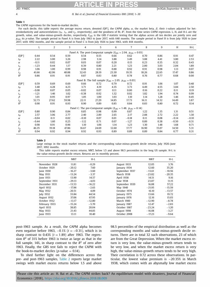
Table 1 reports the monthly CAPM regressions for the
book-to-market deciles. The monthly returns data for the
deciles, the value-weighted market portfolio, and the one-
month Treasury bill rate are from Kenneth French’s data
library. The data are from July 1926 to June 2017.
Panel A shows that, consistent with Fama and French
(1992) , the CAPM has difficulty in explaining the value pre-
mium (the value-minus-growth decile return) in the sam-
ple after July 1963. Moving from the growth decile to the
value decile, the average excess return rises from 0.44% per
month to 0.91%, and the average return spread is 0.47%
( t = 2 . 53 ). Despite the increasing relation between book-
to-market and the average excess return, the market beta
is largely flat across the deciles. The value-minus-growth
decile has only a small market beta of 0.07 ( t = 0 . 86 ). Ac-
cordingly, its CAPM alpha is economically large, 0.43%, al-
beit only marginally significant ( t = 1 . 89 ). The CAPM alpha
is nearly identical in magnitude to the average value pre-
mium. The regression R 2 is essentially zero. The Gibbons
et al. (1989 , GRS) test rejects the null hypothesis that the
alphas across all ten deciles are jointly zero at the 5% sig-
nificance level. 3
Panel B shows that the CAPM explains the value pre-
mium in the long sample from July 1926 to June 2017,
consistent with Ang and Chen (2007) . Their sample ends
in December 2001, and we replicate their result in our
extended sample. The average excess return varies from
0.59% per month for the growth decile to 1.07% for the
value decile. The value premium is, on average, 0.48% ( t =2 . 5 ), which is close to 0.47% in the post-1963 sample. More
important, the CAPM explains the value premium, with a
small alpha of 0.19% ( t = 0 . 99 ) and a large market beta of
0.45 ( t = 3 . 87 ). Relative to the post-1963 sample, the re-
gression R 2 rises considerably from zero to 14%. However,
the GRS test still rejects the null that the CAPM alphas are
jointly zero across the ten deciles.
Panel C shows that the CAPM does a good job in ex-
plaining the value premium from July 1926 to June 1963.
The value-minus-growth decile return is, on average, 0.51%
per month, albeit insignificant ( t = 1 . 3 ). The magnitude of
the value premium is comparable to that in the post-1963
sample. Most important, its market beta is economically
large and statistically significant, 0.71 ( t = 5 . 31 ), in sharp
contrast to the market beta of 0.07 ( t = 0 . 86 ) in the
3 In the original July 1963–December 1990 sample in Fama and French
(1992) , the average excess return goes from 0.22% per month for the
growth decile to 0.81% for the value decile, and the value premium is,
on average, 0.59% ( t = 2 . 41 ) (untabulated). However, the market beta de-
creases slightly from 1.08 for the growth decile to 1.05 for the value
decile. As a result, the CAPM alpha for the value-minus-growth decile is
0.6% ( t = 2 . 17 ).
An equilibrium model with disasters, Journal of Financial
4 H. Bai et al. / Journal of Financial Economics 0 0 0 (2018) 1–30
ARTICLE IN PRESS
JID: FINEC [m3Gdc; September 6, 2018;2:41 ]
Table 1
The CAPM regressions for the book-to-market deciles.
For each decile, this table reports the average excess return, denoted E [ R e ], the CAPM alpha, α, the market beta, β , their t -values adjusted for het-
eroskedasticity and autocorrelations ( t R e , t α , and t β , respectively), and the goodness of fit, R 2 , from the time series CAPM regression. L, H, and H-L are the
growth, value, and value-minus-growth deciles, respectively. F GRS is the GRS F -statistic testing that the alphas across all ten deciles are jointly zero and
p GRS its p -value. The sample period in Panel A is from July 1963 to June 2017, with 648 months. The sample period in Panel B is from July 1926 to June
2017, with 1092 months, and the sample period in Panel C is from July 1926 to June 1963, with 4 4 4 months.
L 2 3 4 5 6 7 8 9 H H-L
Panel A: The post-Compustat sample ( F GRS = 2 . 04 , p GRS = 0 . 03 )
E [ R e ] 0.44 0.54 0.59 0.54 0.55 0.66 0.62 0.70 0.86 0.91 0.47
t R e 2.22 3.00 3.26 2.98 3.14 3.88 3.49 3.88 4.41 3.80 2.53
α −0.11 0.02 0.07 0.03 0.07 0.20 0.15 0.23 0.35 0.32 0.43
t α −1.23 0.44 1.17 0.39 0.80 2.21 1.23 2.00 3.03 2.04 1.89
β 1.06 1.00 0.99 0.98 0.91 0.88 0.92 0.91 0.98 1.13 0.07
t β 41.66 42.06 40.88 32.43 28.19 23.30 19.35 18.26 22.65 17.47 0.86
R 2 0.86 0.91 0.91 0.87 0.83 0.80 0.78 0.76 0.77 0.68 0.00
Panel B: The full sample ( F GRS = 2 . 05 , p GRS = 0 . 03 )
E [ R e ] 0.59 0.69 0.69 0.66 0.72 0.79 0.72 0.91 1.06 1.07 0.48
t R e 3.40 4.28 4.23 3.71 4.19 4.35 3.73 4.49 4.55 3.84 2.50
α −0.08 0.07 0.05 −0.02 0.07 0.11 0.00 0.16 0.22 0.11 0.19
t α −1.21 1.46 1.02 −0.38 0.92 1.32 0.02 1.82 1.94 0.74 0.99
β 1.01 0.95 0.97 1.05 1.00 1.03 1.10 1.14 1.28 1.46 0.45
t β 52.73 27.62 59.98 22.11 27.29 14.85 17.73 16.11 14.32 14.49 3.87
R 2 0.90 0.91 0.93 0.90 0.89 0.85 0.84 0.83 0.80 0.72 0.14
Panel C: The pre-Compustat sample ( F GRS = 1 . 48 , p GRS = 0 . 14 )
E [ R e ] 0.80 0.90 0.84 0.85 0.98 0.99 0.87 1.22 1.35 1.31 0.51
t R e 2.57 3.06 2.77 2.40 2.89 2.65 2.17 2.88 2.72 2.22 1.30
α −0.04 0.11 0.02 −0.10 0.07 0.01 −0.18 0.11 0.08 −0.14 −0.10
t α −0.44 1.60 0.25 −1.12 0.71 0.07 −1.27 0.89 0.38 −0.50 −0.31
β 0.98 0.91 0.96 1.10 1.06 1.14 1.23 1.30 1.48 1.68 0.71
t β 46.35 19.18 47.86 16.67 24.69 12.60 17.77 16.90 15.07 14.50 5.31
R 2 0.94 0.92 0.94 0.92 0.93 0.89 0.89 0.89 0.84 0.77 0.31
Table 2
Large swings in the stock market returns and the corresponding value-minus-growth decile returns, July 1926–June
2017, 1092 months.
This table reports market excess returns, MKT, below 1.5 and above 98.5 percentiles in the long US sample. H-L is
the value-minus-growth decile return. Returns are in monthly percent.
MKT H-L MKT H-L
November 1928 11.81 −0.29 August 1933 12.05 3.76
October 1929 −20.12 7.60 January 1934 12.60 35.20
June 1930 −16.27 −3.60 September 1937 −13.61 −10.56
May 1931 −13.24 −3.37 March 1938 −23.82 −20.35
June 1931 13.90 14.57 April 1938 14.51 9.16
September 1931 −29.13 −4.03 June 1938 23.87 11.15
December 1931 −13.53 −16.22 September 1939 16.88 57.22
April 1932 −17.96 −2.65 May 1940 −21.95 −15.59
May 1932 −20.51 4.09 October 1974 16.10 −13.57
July 1932 33.84 44.54 January 1975 13.66 19.72
August 1932 37.06 67.95 January 1976 12.16 15.03
October 1932 −13.17 −12.80 March 1980 −12.90 −8.78
February 1933 −15.24 −5.70 January 1987 12.47 −2.83
April 1933 38.85 20.04 October 1987 −23.24 −1.20
May 1933 21.43 44.85 August 1998 −16.08 −3.27
June 1933 13.11 10.40 October 2008 −17.23 −9.64
post-1963 sample. As a result, the CAPM alpha becomes
even negative before 1963, −0 . 1% ( t = −0 . 31 ), which is in
sharp contrast to 0.43% ( t = 1 . 89 ) after 1963. The regres-
sion R 2 of 31% before 1963 is twice as large as that in the
full sample, 14%, in sharp contrast to the R 2 of zero after
1963. Finally, the GRS test fails to reject the CAPM with
the book-to-market deciles ( p -value = 0.14).
To shed further light on the differences across the
pre- and post-1963 samples, Table 2 reports large market
swings with market excess returns below 1.5 and above
Please cite this article as: H. Bai et al., The CAPM strikes back?
Economics (2018), https://doi.org/10.1016/j.jfineco.2018.08.009
98.5 percentiles of the empirical distribution as well as the
corresponding months and value-minus-growth decile re-
turns. There are in total 32 such observations, 23 of which
are from the Great Depression. When the market excess re-
turn is very low, the value-minus-growth return tends to
be very low, and when the market excess return is very
high, the value-minus-growth return tends to be very high.
Their correlation is 0.72 across these observations. In par-
ticular, the lowest value premium is −20 . 35% in March
1938, which comes with an abysmally low market excess
An equilibrium model with disasters, Journal of Financial

H. Bai et al. / Journal of Financial Economics 0 0 0 (2018) 1–30 5
ARTICLE IN PRESS
JID: FINEC [m3Gdc; September 6, 2018;2:41 ]
Fig. 1. The CAPM regressions for the value-minus-growth decile, July 1926–June 2017. The figure presents the scatter plot and fitted line for the time series
CAPM regression of the value premium, defined as the value-minus-growth decile return. In Panel A, the monthly market excess returns below the 1.5 and
above 98.5 percentiles are dated in red. Returns are in monthly percent. The sample period in Panel A is from July 1926 to June 2017, with 1092 months,
and the sample period in Panel B is from July 1963 to June 2017, with 648 months. (For interpretation of the references to color in this figure legend, the
reader is referred to the web version of this article.)
return of −23 . 82% . The highest value premium is 67.95% in
August 1932, which comes with an exuberantly high mar-
ket excess return of 37.06%. More recently, following the
bankruptcy of Lehman Brothers, the market excess return
is −17.23% in October 2008, during which the value-minus-
growth return is −9 . 64% .
Fig. 1 presents the scatter plots and fitted market re-
gression lines for the value-minus-growth decile return for
the long sample (Panel A) and the post-1963 sample (Panel
B). Panel A highlights in red the observations with monthly
market excess returns below 1.5 and above 98.5 percentiles
of the empirical distribution. These observations clearly
contribute to the market beta of 0.45 ( t = 3 . 87 ) for the
value-minus-growth decile in the long sample. In contrast,
Panel B shows that large swings in the stock market are
scarce in the post-1963 sample, giving rise to a largely flat
regression line. In all, the CAPM does a good job in ex-
plaining the value premium in the long sample that in-
cludes the Great Depression but largely fails in the short
post-1963 sample.
2.2. The beta anomaly
Refuting Ang and Chen (2007) , who argue that the
CAPM explains the value premium in the long sample,
Fama and French (2006) emphasize the CAPM’s problem
that the cross-sectional variation in the market beta goes
unrewarded. This flat relation between the market beta
and the average return, known as the beta anomaly, has
a long tradition in empirical asset pricing ( Fama and Mac-
Beth, 1973; Fama and French, 1992; Frazzini and Pedersen,
2014 ).
Table 3 presents the average excess returns and CAPM
regressions across the market beta deciles. At the end of
June of each year t , NYSE, Amex, and Nasdaq stocks are
Please cite this article as: H. Bai et al., The CAPM strikes back?
Economics (2018), https://doi.org/10.1016/j.jfineco.2018.08.009
sorted into deciles based on the NYSE breakpoints of the
preranking betas from rolling-window CAPM regressions
in the prior 60 months (24 months minimum). Monthly
value-weighted returns are calculated from July of year t
to June of t + 1 , and the deciles are rebalanced in June.
The sample starts in July 1928 because we use the data
from the first 24 months to estimate the preranking betas
in June 1928.
Panel A shows that, contradicting the CAPM, the re-
lation between the market beta and the average return
in the data is largely flat. Moving from the low to high
beta decile, the average excess return rises from 0.52% per
month to 0.55%, and the tiny spread of 0.03% is within
0.2 standard errors from zero. Sorting on the preranking
beta yields an economically large postranking beta spread
of 1.06 ( t = 11 . 81 ) across the extreme deciles. As such, the
CAPM alpha for the high-minus-low market beta decile
is economically large, −0 . 52% , albeit marginally significant
( t = −1 . 94 ).
From Panel B, the sample from July 1928 onward yields
largely similar results. The average excess return varies
from 0.58% per month for the low beta decile to 0.75%
for the high beta decile, and the small spread of 0.16%
is within one standard error from zero. The preranking
beta sort again yields an economically large spread of
1.13 ( t = 18 . 82 ) in the postranking beta across the extreme
deciles. As such, the CAPM alpha for the high-minus-low
beta decile is negative, both economically large, −0 . 55% ,
and statistically significant ( t = −2 . 81 ).
2.3. The failure of the consumption CAPM
To test the consumption CAPM, we use two-stage
Fama and MacBeth (1973) cross-sectional regressions be-
cause the aggregate consumption growth is not tradable
An equilibrium model with disasters, Journal of Financial

6 H. Bai et al. / Journal of Financial Economics 0 0 0 (2018) 1–30
ARTICLE IN PRESS
JID: FINEC [m3Gdc; September 6, 2018;2:41 ]
Table 3
The CAPM regressions for the preranking market beta deciles.
For each decile, this table reports the average excess return, E [ R e ], the CAPM alpha, α, the postranking market beta, β , t -statistics adjusted for het-
eroskedasticity and autocorrelations ( t R e , t α , and t β , respectively), and the goodness of fit, R 2 , from the time series CAPM regressions. L, H, and H-L are the
low, high, and high-minus-low preranking market beta decile. F GRS is the GRS F -statistic testing that the alphas across all ten deciles are jointly zero and
p GRS its p -value. The sample period in Panel A is from July 1963 to June 2017, with 648 months. The sample period in Panel B is from July 1928 to June
2017, with 1068 months, with the 24 monthly observations from July 1926 to June 1928 used to estimate the market betas for July 1928.
L 2 3 4 5 6 7 8 9 H H-L
Panel A: The post-Compustat sample ( F GRS = 1 . 39 , p GRS = 0 . 18 )
E [ R e ] 0.52 0.52 0.56 0.58 0.69 0.55 0.67 0.55 0.57 0.55 0.03
t R e 3.85 3.64 3.45 3.38 3.75 2.86 3.14 2.42 2.23 1.72 0.11
α 0.22 0.17 0.13 0.12 0.18 0.01 0.07 −0.08 −0.13 −0.29 −0.52
t α 2.11 1.76 1.69 1.42 2.17 0.18 0.85 −0.82 −1.10 −1.49 −1.94
β 0.57 0.68 0.82 0.87 0.98 1.03 1.15 1.22 1.34 1.62 1.06
t β 12.39 17.21 20.57 20.68 28.13 31.21 50.25 41.76 35.41 30.92 11.81
R 2 0.53 0.68 0.77 0.79 0.86 0.86 0.88 0.86 0.84 0.77 0.43
Panel B: The full sample ( F GRS = 2 . 41 , p GRS = 0 . 01 )
E [ R e ] 0.58 0.63 0.65 0.74 0.83 0.72 0.79 0.73 0.77 0.75 0.16
t R e 5.03 4.66 4.41 4.46 4.54 3.71 3.74 3.11 2.94 2.44 0.66
α 0.22 0.16 0.13 0.14 0.17 0.01 0.02 −0.13 −0.17 −0.33 −0.55
t α 2.87 2.22 2.21 2.31 2.49 0.20 0.27 −1.51 −1.68 −2.29 −2.81
β 0.57 0.73 0.83 0.94 1.05 1.11 1.22 1.36 1.48 1.70 1.13
t β 22.86 30.50 36.61 40.31 41.41 39.61 48.26 36.17 26.65 40.93 18.82
R 2 0.66 0.81 0.85 0.88 0.90 0.90 0.91 0.90 0.88 0.84 0.57
( Breeden et al., 1989; Jagannathan and Wang, 2007 ). To
ensure a sufficient number of observations in the second-
stage regressions, we use the 25 size and book-to-market
portfolios as testing assets ( Fama and French, 1996 ). In the
first stage, we regress excess returns on the aggregate con-
sumption growth, g Ct :
R
e it = a i + βC
i g Ct + e it , (1)
in which R e it
is portfolio i ’s excess return, βC i
the consump-
tion beta, and e it the residual.
In the second stage, we regress portfolio excess returns
on the consumption betas:
R
e it = φ0 + φ1 β
C i + αi , (2)
in which φ0 is the intercept, φ1 the price of consump-
tion risk, and αi the residual. The consumption CAPM pre-
dicts that φ0 + αi = 0 , φ1 is significantly positive, and the
expected risk premium equals φ1 βC i
. We test φ0 + αi = 0
with a χ2 -test, which is the cross-sectional counterpart of
the time series GRS test, following Eq. (12.14) in Cochrane
(2005b) . We adjust the variance-covariance matrix of the
pricing errors with the Shanken (1992) method per Eq.
(12.20) in Cochrane (2005b) .
We obtain consumption data from National Income and
Product Accounts (NIPA) Table 7.1 from Bureau of Eco-
nomic Analysis. Consumption is the sum of per capita non-
durables plus services in chained dollars. The annual se-
ries is from 1929 to 2016, and the quarterly series from
the first quarter (Q1) of 1947 to the second quarter (Q2)
of 2017. The annual series contains the Great Depression
but the quarterly series does not. We test the consumption
CAPM with both annual and quarterly data. We also im-
plement the Jagannathan and Wang (2007) fourth-quarter
consumption growth model, in which annual consump-
tion growth is calculated with only the fourth-quarter con-
sumption data. The rationale is that investors are more
likely to make their consumption and portfolio choice deci-
Please cite this article as: H. Bai et al., The CAPM strikes back?
Economics (2018), https://doi.org/10.1016/j.jfineco.2018.08.009
sions simultaneously in the fourth-quarter because the tax
year ends in December.
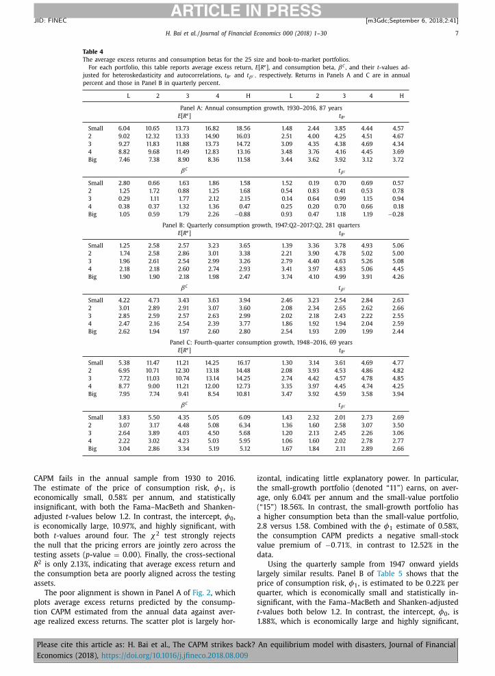
Table 4 reports the average excess returns and con-
sumption betas for the 25 size and book-to-market portfo-
lios. The portfolio returns data are from Kenneth French’s
website. Panel A shows that in the 1930–2016 annual sam-
ple, the average value premium is stronger in small firms
than in big firms. In the smallest quintile, the value-minus-
growth quintile return is, on average, 12.52% per annum
( t = 4 . 31 ), whereas in the biggest quintile, only 4.12% ( t =1 . 74 ). The pattern is similar in the 1947:Q2–2017:Q2 quar-
terly sample. The value premium is, on average, 2.4% per
quarter ( t = 5 . 01 ) in the smallest quintile but only 0.57%
( t = 1 . 33 ) in the biggest quintile. The results from the
shorter 1948–2016 annual sample are largely similar.
Panel A also shows that the consumption betas es-
timated from annual consumption growth do not align
with the average returns across the 25 portfolios. For
example, despite the high average excess return, 18.56%
per annum, of the small-value portfolio, relative to only
6.04% of the small-growth portfolio, the consumption
beta of the former is lower than that of the latter, 1.58
versus 2.8. Similarly, Panel B shows that the consumption
betas estimated from quarterly consumption growth do
not align either with the average returns. The contrast in
the average return between the small-growth and small-
value portfolios is 1.25% versus 3.65% per quarter, but the
consumption beta goes in the wrong direction, 4.22 ver-
sus 3.94. Finally, consistent with Jagannathan and Wang
(2007) , the consumption betas estimated from fourth-
quarter consumption growth align better with the average
returns. The small-value portfolio has a consumption beta
of 6.09, which is higher than 3.83 of the small-growth
portfolio, going in the right direction in explaining the
average returns.
Table 5 reports the second-stage cross-sectional tests
of the consumption CAPM. From Panel A, the consumption
An equilibrium model with disasters, Journal of Financial
H. Bai et al. / Journal of Financial Economics 0 0 0 (2018) 1–30 7
ARTICLE IN PRESS
JID: FINEC [m3Gdc; September 6, 2018;2:41 ]
Table 4
The average excess returns and consumption betas for the 25 size and book-to-market portfolios.
For each portfolio, this table reports average excess return, E [ R e ], and consumption beta, βC , and their t -values ad-
justed for heteroskedasticity and autocorrelations, t R e and t βC , respectively. Returns in Panels A and C are in annual
percent and those in Panel B in quarterly percent.
L 2 3 4 H L 2 3 4 H
Panel A: Annual consumption growth, 1930–2016, 87 years
E [ R e ] t R e
Small 6.04 10.65 13.73 16.82 18.56 1.48 2.44 3.85 4.44 4.57
2 9.02 12.32 13.33 14.90 16.03 2.51 4.00 4.25 4.51 4.67
3 9.27 11.83 11.88 13.73 14.72 3.09 4.35 4.38 4.69 4.34
4 8.82 9.68 11.49 12.83 13.16 3.48 3.76 4.16 4.45 3.69
Big 7.46 7.38 8.90 8.36 11.58 3.44 3.62 3.92 3.12 3.72
βC t βC
Small 2.80 0.66 1.63 1.86 1.58 1.52 0.19 0.70 0.69 0.57
2 1.25 1.72 0.88 1.25 1.68 0.54 0.83 0.41 0.53 0.78
3 0.29 1.11 1.77 2.12 2.15 0.14 0.64 0.99 1.15 0.94
4 0.38 0.37 1.32 1.36 0.47 0.25 0.20 0.70 0.66 0.18
Big 1.05 0.59 1.79 2.26 −0.88 0.93 0.47 1.18 1.19 −0.28
Panel B: Quarterly consumption growth, 1947:Q2–2017:Q2, 281 quarters
E [ R e ] t R e
Small 1.25 2.58 2.57 3.23 3.65 1.39 3.36 3.78 4.93 5.06
2 1.74 2.58 2.86 3.01 3.38 2.21 3.90 4.78 5.02 5.00
3 1.96 2.61 2.54 2.99 3.26 2.79 4.40 4.63 5.26 5.08
4 2.18 2.18 2.60 2.74 2.93 3.41 3.97 4.83 5.06 4.45
Big 1.90 1.90 2.18 1.98 2.47 3.74 4.10 4.99 3.91 4.26
βC t βC
Small 4.22 4.73 3.43 3.63 3.94 2.46 3.23 2.54 2.84 2.63
2 3.01 2.89 2.91 3.07 3.60 2.08 2.34 2.65 2.62 2.66
3 2.85 2.59 2.57 2.63 2.99 2.02 2.18 2.43 2.22 2.55
4 2.47 2.16 2.54 2.39 3.77 1.86 1.92 1.94 2.04 2.59
Big 2.62 1.94 1.97 2.60 2.80 2.54 1.93 2.09 1.99 2.44
Panel C: Fourth-quarter consumption growth, 1948–2016, 69 years
E [ R e ] t R e
Small 5.38 11.47 11.21 14.25 16.17 1.30 3.14 3.61 4.69 4.77
2 6.95 10.71 12.30 13.18 14.48 2.08 3.93 4.53 4.86 4.82
3 7.72 11.03 10.74 13.14 14.25 2.74 4.42 4.57 4.78 4.85
4 8.77 9.00 11.21 12.00 12.73 3.35 3.97 4.45 4.74 4.25
Big 7.95 7.74 9.41 8.54 10.81 3.47 3.92 4.59 3.58 3.94
βC t βC
Small 3.83 5.50 4.35 5.05 6.09 1.43 2.32 2.01 2.73 2.69
2 3.07 3.17 4.48 5.08 6.34 1.36 1.60 2.58 3.07 3.50
3 2.64 3.89 4.03 4.50 5.68 1.20 2.13 2.45 2.26 3.06
4 2.22 3.02 4.23 5.03 5.95 1.06 1.60 2.02 2.78 2.77
Big 3.04 2.86 3.34 5.19 5.12 1.67 1.84 2.11 2.89 2.66
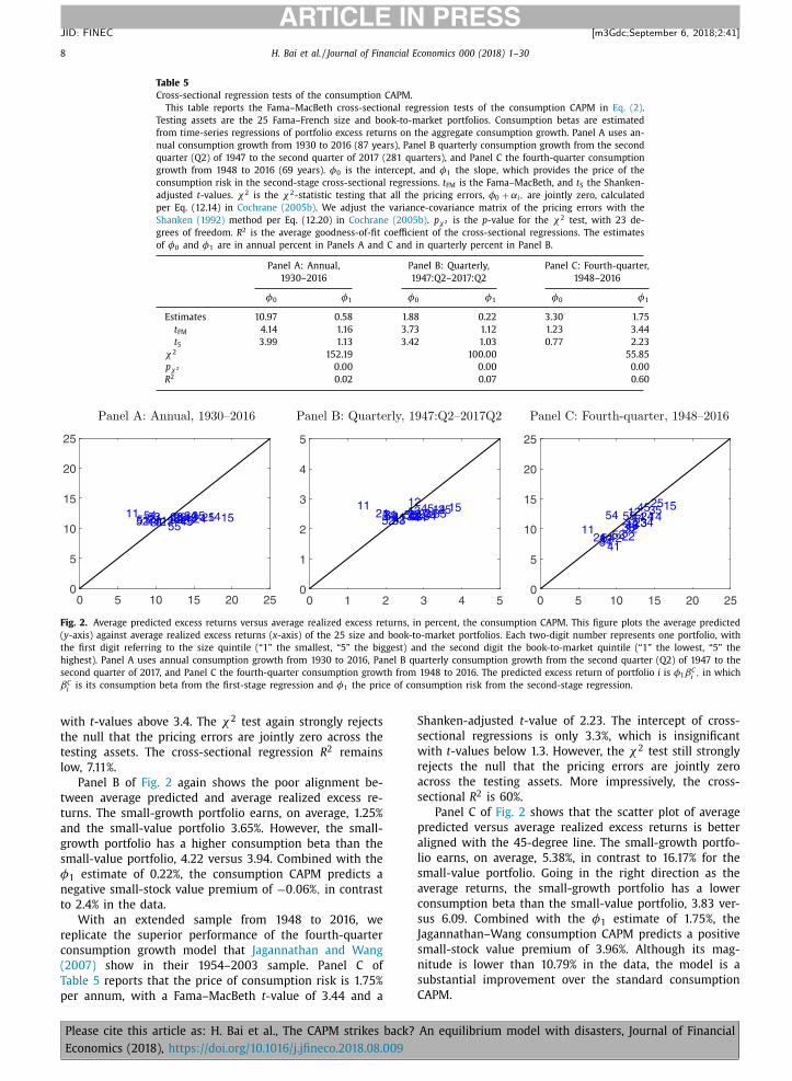
CAPM fails in the annual sample from 1930 to 2016.
The estimate of the price of consumption risk, φ1 , is
economically small, 0.58% per annum, and statistically
insignificant, with both the Fama–MacBeth and Shanken-
adjusted t -values below 1.2. In contrast, the intercept, φ0 ,
is economically large, 10.97%, and highly significant, with
both t -values around four. The χ2 test strongly rejects
the null that the pricing errors are jointly zero across the
testing assets ( p -value = 0.00). Finally, the cross-sectional
R 2 is only 2.13%, indicating that average excess return and
the consumption beta are poorly aligned across the testing
assets.
The poor alignment is shown in Panel A of Fig. 2 , which
plots average excess returns predicted by the consump-
tion CAPM estimated from the annual data against aver-
age realized excess returns. The scatter plot is largely hor-
Please cite this article as: H. Bai et al., The CAPM strikes back?
Economics (2018), https://doi.org/10.1016/j.jfineco.2018.08.009
izontal, indicating little explanatory power. In particular,
the small-growth portfolio (denoted “11”) earns, on aver-
age, only 6.04% per annum and the small-value portfolio
(“15”) 18.56%. In contrast, the small-growth portfolio has
a higher consumption beta than the small-value portfolio,
2.8 versus 1.58. Combined with the φ1 estimate of 0.58%,
the consumption CAPM predicts a negative small-stock
value premium of −0 . 71% , in contrast to 12.52% in the
data.
Using the quarterly sample from 1947 onward yields
largely similar results. Panel B of Table 5 shows that the
price of consumption risk, φ1 , is estimated to be 0.22% per
quarter, which is economically small and statistically in-
significant, with the Fama–MacBeth and Shanken-adjusted
t -values both below 1.2. In contrast, the intercept, φ0 , is
1.88%, which is economically large and highly significant,
An equilibrium model with disasters, Journal of Financial
8 H. Bai et al. / Journal of Financial Economics 0 0 0 (2018) 1–30
ARTICLE IN PRESS
JID: FINEC [m3Gdc; September 6, 2018;2:41 ]
Table 5
Cross-sectional regression tests of the consumption CAPM.
This table reports the Fama–MacBeth cross-sectional regression tests of the consumption CAPM in Eq. (2) .
Testing assets are the 25 Fama–French size and book-to-market portfolios. Consumption betas are estimated
from time-series regressions of portfolio excess returns on the aggregate consumption growth. Panel A uses an-
nual consumption growth from 1930 to 2016 (87 years), Panel B quarterly consumption growth from the second
quarter (Q2) of 1947 to the second quarter of 2017 (281 quarters), and Panel C the fourth-quarter consumption
growth from 1948 to 2016 (69 years). φ0 is the intercept, and φ1 the slope, which provides the price of the
consumption risk in the second-stage cross-sectional regressions. t FM is the Fama–MacBeth, and t S the Shanken-
adjusted t -values. χ2 is the χ2 -statistic testing that all the pricing errors, φ0 + αi , are jointly zero, calculated
per Eq. (12.14) in Cochrane (2005b) . We adjust the variance-covariance matrix of the pricing errors with the
Shanken (1992) method per Eq. (12.20) in Cochrane (2005b) . p χ2 is the p -value for the χ2 test, with 23 de-
grees of freedom. R 2 is the average goodness-of-fit coefficient of the cross-sectional regressions. The estimates
of φ0 and φ1 are in annual percent in Panels A and C and in quarterly percent in Panel B.
Panel A: Annual, Panel B: Quarterly, Panel C: Fourth-quarter,
1930–2016 1947:Q2–2017:Q2 1948–2016
φ0 φ1 φ0 φ1 φ0 φ1
Estimates 10.97 0.58 1.88 0.22 3.30 1.75
t FM 4.14 1.16 3.73 1.12 1.23 3.44
t S 3.99 1.13 3.42 1.03 0.77 2.23
χ2 152.19 10 0.0 0 55.85
p χ2 0.00 0.00 0.00
R 2 0.02 0.07 0.60
Fig. 2. Average predicted excess returns versus average realized excess returns, in percent, the consumption CAPM. This figure plots the average predicted
( y -axis) against average realized excess returns ( x -axis) of the 25 size and book-to-market portfolios. Each two-digit number represents one portfolio, with
the first digit referring to the size quintile (“1” the smallest, “5” the biggest) and the second digit the book-to-market quintile (“1” the lowest, “5” the
highest). Panel A uses annual consumption growth from 1930 to 2016, Panel B quarterly consumption growth from the second quarter (Q2) of 1947 to the
second quarter of 2017, and Panel C the fourth-quarter consumption growth from 1948 to 2016. The predicted excess return of portfolio i is φ1 βC i , in which
βC i
is its consumption beta from the first-stage regression and φ1 the price of consumption risk from the second-stage regression.
with t -values above 3.4. The χ2 test again strongly rejects
the null that the pricing errors are jointly zero across the
testing assets. The cross-sectional regression R 2 remains
low, 7.11%.
Panel B of Fig. 2 again shows the poor alignment be-
tween average predicted and average realized excess re-
turns. The small-growth portfolio earns, on average, 1.25%
and the small-value portfolio 3.65%. However, the small-
growth portfolio has a higher consumption beta than the
small-value portfolio, 4.22 versus 3.94. Combined with the
φ1 estimate of 0.22%, the consumption CAPM predicts a
negative small-stock value premium of −0 . 06% , in contrast
to 2.4% in the data.
With an extended sample from 1948 to 2016, we
replicate the superior performance of the fourth-quarter
consumption growth model that Jagannathan and Wang
(2007) show in their 1954–2003 sample. Panel C of
Table 5 reports that the price of consumption risk is 1.75%
per annum, with a Fama–MacBeth t -value of 3.44 and a
Please cite this article as: H. Bai et al., The CAPM strikes back?
Economics (2018), https://doi.org/10.1016/j.jfineco.2018.08.009
Shanken-adjusted t -value of 2.23. The intercept of cross-
sectional regressions is only 3.3%, which is insignificant
with t -values below 1.3. However, the χ2 test still strongly
rejects the null that the pricing errors are jointly zero
across the testing assets. More impressively, the cross-
sectional R 2 is 60%.
Panel C of Fig. 2 shows that the scatter plot of average
predicted versus average realized excess returns is better
aligned with the 45-degree line. The small-growth portfo-
lio earns, on average, 5.38%, in contrast to 16.17% for the
small-value portfolio. Going in the right direction as the
average returns, the small-growth portfolio has a lower
consumption beta than the small-value portfolio, 3.83 ver-
sus 6.09. Combined with the φ1 estimate of 1.75%, the
Jagannathan–Wang consumption CAPM predicts a positive
small-stock value premium of 3.96%. Although its mag-
nitude is lower than 10.79% in the data, the model is a
substantial improvement over the standard consumption
CAPM.
An equilibrium model with disasters, Journal of Financial

H. Bai et al. / Journal of Financial Economics 0 0 0 (2018) 1–30 9
ARTICLE IN PRESS
JID: FINEC [m3Gdc; September 6, 2018;2:41 ]
U
Y
4 Kopecky and Suen (2010) show that the Rouwenhorst (1995) method
dominates other popular methods in the Markov-chain approximation to
autoregressive processes in the context of the stochastic growth model.
Petrosky-Nadeau and Zhang (2017) show similar results in the search
model of equilibrium unemployment. 5 To construct the P matrix, we set p = (ρg + 1) / 2 , and define the tran-
sition matrix for n g = 3 as
˜ P (3) ≡[
p 2 2 p(1 − p) (1 − p) 2
p(1 − p) p 2 + (1 − p) 2 p(1 − p) (1 − p) 2 2 p(1 − p) p 2
] . (11)
To obtain P =
P (5) , we use the following recursion:
p
[˜ P (n g ) 0
0 ′ 0
]+ (1 − p)
[0 ˜ P (n g )
0 0 ′
]+ (1 − p)
[0 ′ 0 ˜ P (n g ) 0
]+ p
[0 0 ′ 0 ˜ P (n g )
],
(12)
in which 0 is a n g × 1 column vector of zeros. We then divide all but the
top and bottom rows by two to ensure that the conditional probabilities
sum up to one in ˜ P (n g +1) (see Rouwenhorst, 1995 , p. 306–307, p. 325–
329).
3. An equilibrium model
Our general equilibrium model with disasters and het-
erogeneous firms draws elements from the disaster model
of Rietz (1988) and Barro (2006, 2009) as well as the neo-
classical investment model of Zhang (2005) . The economy
is populated by a representative household with recursive
utility and heterogenous firms. The firms take the house-
hold’s intertemporal rate of substitution as given when de-
termining optimal policies. The production technology is
subject to both aggregate and firm-specific shocks. The ag-
gregate shock contains normally distributed states as well
as a disaster and a recovery state.
3.1. Preferences
The representative household has recursive utility, U t ,
defined over aggregate consumption, C t :
t =
[(1 − �) C
1 − 1 ψ
t + �
(E t [U
1 −γt+1
]) 1 −1 /ψ 1 −γ
] 1 1 −1 /ψ
, (3)
in which ϱ is the time discount factor, ψ the intertemporal
elasticity of substitution, and γ the relative risk aversion
( Epstein and Zin, 1989 ). The pricing kernel is given by
M t+1 = �
(C t+1
C t
)− 1 ψ
(
U
1 −γt+1
E t [U
1 −γt+1
])
1 /ψ−γ1 −γ
. (4)
We adopt the recursive utility to delink the relative risk
aversion, γ , from the intertemporal elasticity of substitu-
tion, ψ . Their values are both higher than unity in our
calibration ( Section 4.1 ). Nakamura et al. (2013) show that
a low value of ψ less than unity implies counterfactually
a surge in stock prices at the onset of disasters. The rea-
son is that entering a (persistent) disaster state generates
a strong desire to save, since consumption is expected to
fall substantially in the future. With a small ψ , this effect
dominates the negative effect of the disaster state on firms’
cash flows, raising their stock prices. Gourio (2012) makes
a similar point in a production economy that when ψ < 1,
the onset of disasters counterfactually increases invest-
ment.
3.2. Technology
Firms produce output with capital and are subject to
both aggregate and firm-specific shocks. Output for firm i
at time t , denoted Y it ≡ Y ( K it , Z it , X t ), is given by
it = (X t Z it ) 1 −ξ K
ξit , (5)
in which ξ > 0 is the curvature parameter, X t is the aggre-
gate productivity, Z it is the firm-specific productivity, and
K it is capital. Operating profits, denoted it , are defined as
it = Y it − f K it , (6)
in which fK it , with f > 0, is the fixed costs of produc-
tion. The fixed costs are scaled by capital to ensure that
the costs do not become trivially small along a balanced
growth path.
Please cite this article as: H. Bai et al., The CAPM strikes back?
Economics (2018), https://doi.org/10.1016/j.jfineco.2018.08.009
The log aggregate productivity growth, g xt ≡log (X t /X t−1 ) , is specified as
g xt = g + g t , (7)
in which g is the constant mean. We assume that g t follows
a first-order autoregressive process:
g t+1 = ρg g t + σg εg t+1
, (8)
in which εg t+1
is a standard normal shock, and the uncon-
ditional mean of g t is zero.
The firm-specific productivity for firm i , Z it , has a tran-
sition function given by
z it+1 = (1 − ρz ) z + ρz z it + σz εz it+1 , (9)
in which z it ≡ log Z it , z is the unconditional mean of z itcommon to all firms, and εz
it+1 is an independently and
identically distributed standard normal shock. We assume
that εz it+1
and εz jt+1
are uncorrelated for any i � = j , and εg t+1
and εz it+1
are uncorrelated for all i .
3.3. Disasters
We follow Rouwenhorst (1995) to discretize the de-
meaned aggregate productivity growth, g t , into a five-point
grid, { g 1 , g 2 , g 3 , g 4 , g 5 }. 4 The grid is symmetric around
the long-run mean of zero and even spaced. The dis-
tance between any two adjacent grid point is given by
2 σg / √
(1 − ρ2 g )(n g − 1) , in which n g = 5 . The Rouwenhorst
procedure also produces a transition matrix, ˜ P , given by
˜ P =
⎡ ⎢ ⎢ ⎣
p 11 p 12 . . . p 15
p 21 p 22 . . . p 25
. . . . . .
. . . . . .
p 51 p 52 . . . p 55
⎤ ⎥ ⎥ ⎦
, (10)
in which p ij , for i, j = 1 , . . . , 5 , is the probability of g t+1 =g j conditional on g t = g i .
5
Alternatively, instead of the autoregressive process of
g t in Eq. (8) , we could specify g t directly as the five-
state Markov process with the transition matrix given by˜ P . The benefit of starting from the autoregressive process
An equilibrium model with disasters, Journal of Financial
10 H. Bai et al. / Journal of Financial Economics 0 0 0 (2018) 1–30
ARTICLE IN PRESS
JID: FINEC [m3Gdc; September 6, 2018;2:41 ]
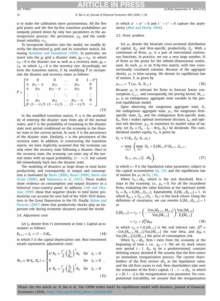
is to make the calibration more parsimonious. All the five
grid points and the five-by-five transition probabilities are
uniquely pinned down by only two parameters in the au-
toregressive process: the persistence, ρg , and the condi-
tional volatility, σ g .
To incorporate disasters into the model, we modify di-
rectly the discretized g t grid and its transition matrix, fol-
lowing Danthine and Donaldson (1999) . In particular, we
insert into the g t grid a disaster state, g 0 = λD , in which
λD < 0 is the disaster size as well as a recovery state, g 6 =
λR , in which λR > 0 is the recovery size. Accordingly, we
form the transition matrix, P , by modifying ˜ P to incorpo-
rate the disaster and recovery states as follows:
P =
⎡ ⎢ ⎢ ⎢ ⎢ ⎢ ⎣
θ 0 0 . . . 0 1 − θη p 11 − η p 12 . . . p 15 0
η p 21 p 22 − η . . . p 25 0
. . . . . .
. . . . . .
. . . . . .
η p 51 p 52 . . . p 55 − η 0
0 (1 − ν) / 5 (1 − ν) / 5 . . . (1 − ν) / 5 ν
⎤ ⎥ ⎥ ⎥ ⎥ ⎥ ⎦
.
(13)
In the modified transition matrix, P , η is the probabil-
ity of entering the disaster state from any of the normal
states, and θ is the probability of remaining in the disaster
state next period conditional on the economy in the disas-
ter state in the current period. As such, θ is the persistence
of the disaster state. Similarly, ν is the persistence of the
recovery state. In addition, in constructing the transition
matrix, we have implicitly assumed that the economy can
only enter the recovery state following a disaster. Once in
the recovery state, the economy can enter any of the nor-
mal states with an equal probability, (1 − ν) / 5 , but cannot
fall immediately back into the disaster state.
The modeling of disasters as large drops in total factor
productivity, and consequently, in output and consump-
tion is motivated by Barro (2006) , Barro (2009) , Barro and
Ursúa (2008) , and Nakamura et al. (2013) . These studies
show evidence on consumption and output disasters in a
historical cross-country panel. In addition, Cole and Oha-
nian (1999) show that negative shocks to total factor pro-
ductivity can account for over half of the 1929–1933 down-
turn in the Great Depression in the US. Finally, Kehoe and
Prescott (2007) show that productivity shocks play an im-
portant role during economic disasters around the world.
3.4. Adjustment costs
Let I it denote firm i ’s investment at time t . Capital accu-
mulates as follows:
K it+1 = I it + (1 − δ) K it , (14)
in which δ is the capital depreciation rate. Real investment
entails asymmetric adjustment costs:
�it ≡ �(I it , K it ) =
⎧ ⎪ ⎪ ⎪ ⎨ ⎪ ⎪ ⎪ ⎩
a + K it +
c +
2
(I it K it
)2
K it for I it > 0
0 for I it = 0
a −K it +
c −
2
(I it K it
)2
K it for I it < 0
,
(15)
Please cite this article as: H. Bai et al., The CAPM strikes back?
Economics (2018), https://doi.org/10.1016/j.jfineco.2018.08.009
in which a − > a + > 0 and c − > c + > 0 capture the asym-
metry ( Abel and Eberly, 1994 ).
3.5. Firms’ problem
Let μt denote the bivariate cross-sectional distribution
of capital, K it , and firm-specific productivity, Z it . With a
continuum of firms, μt is a pair of interrelated continu-
ous functions. In practice, we use a very large number, N ,
of firms as the proxy for the infinite-dimensional contin-
uum. As such, μt is an N -by-two matrix, with two cross-
sectionally correlated columns. Because of the aggregate
shocks, μt is time-varying. We denote its equilibrium law
of motion, Y, as given by
μt+1 = ϒ(μt , X t , X t+1 ) . (16)
Because μt is relevant for firms to forecast future con-
sumption, C t+1 , and consequently, the pricing kernel, M t+1 ,
μt is an endogenous, aggregate state variable in the gen-
eral equilibrium model.
Upon observing the exogenous aggregate state, X t ,
the endogenous aggregate state, μt , the exogenous firm-
specific state, Z it , and the endogenous firm-specific state,
K it , firm i makes optimal investment decision, I it , and opti-
mal exit decision, χ it , to maximize its market value of eq-
uity. Let D it ≡ it − I it − �(I it , K it ) be dividends. The cum-
dividend market equity, V it , is given by
V it ≡ V (K it , Z it ; X t , μt )
= max { χit }
(max { I it }
D it + E t [ M t+1 V (K it+1 , Z it+1 ;
X t+1 , μt+1 )] , sK it
), (17)
in which s > 0 is the liquidation value parameter, subject to
the capital accumulation Eq. (14) and the equilibrium law
of motion for μt in Eq. (16) .
When V it ≥ sK it , which is the exit threshold, firm i
stays in the economy, i.e., χit = 0 . For all the incumbent
firms, evaluating the value function at the optimum yields
V it = D it + E t [ M t+1 V it+1 ] . Equivalently, E t [ M t+1 R it+1 ] = 1 , in
which R it+1 ≡ V it+1 / (V it − D it ) is the stock return. Using the
definition of covariance, we can rewrite E t [ M t+1 R it+1 ] = 1
as
E t [ R it+1 ] = r f t +
(−Cov t [ R it+1 , M t+1 ]
Var t [ M t+1 ]
)Var t [ M t+1 ]
E t [ M t+1 ]
= r f t + βM
it φMt (18)
in which r f t ≡ 1 /E t [ M t+1 ] is the real interest rate, βM
i ≡
−Cov t [ R it+1 , M t+1 ] / Var t [ M t+1 ] the true beta, and φMt ≡Var t [ M t+1 ] / E t [ M t+1 ] the price of consumption risk.
When V it < sK it , firm i exits from the economy at the
beginning of time t , i.e., χit = 1 . We set its stock return
over period t − 1 , R it , to be a predetermined, constant
delisting return, denoted
R . We assume that the firm enters
an immediate reorganization process. The current share-
holders of the firm receive sK it as the liquidation value,
and the old firm ceases to exit. New shareholders take over
the remainder of the firm’s capital, (1 − s − κ) K it , in which
κ ∈ [0 , 1 − s ] is the reorganization cost parameter. For com-
putational tractability, we assume that the reorganization
An equilibrium model with disasters, Journal of Financial

H. Bai et al. / Journal of Financial Economics 0 0 0 (2018) 1–30 11
ARTICLE IN PRESS
JID: FINEC [m3Gdc; September 6, 2018;2:41 ]
V
C
process occurs instantaneously. At the beginning of t , the
old firm is replaced by a new firm with an initial capital
of (1 − s − κ) K it and a new firm-specific log productivity,
z it , that equals its unconditional mean, z . This modeling of
entry and exit keeps the number of firms constant in the
economy.
Prior theoretical models, all of which have no disasters,
have largely ignored the exit decision. With disasters, firms
are more likely to exit in the disaster state, especially when
the liquidation value parameter, s , is high. As such, we in-
corporate the exit decision, and the related entry decision,
into the model to better quantify the impact of disaster dy-
namics on the cross-section.
3.6. Competitive equilibrium
A recursive competitive equilibrium consists of an op-
timal investment rule, I ( K it , Z it ; X t , μt ); an optimal exit
rule, χ ( K it , Z it ; X t , μt ); a value function, V ( K it , Z it ; X t , μt );
and an equilibrium law of motion for the firm distribution,
ϒ(μt , X t , X t+1 ) , such that the following conditions hold.
• Optimality: I ( K it , Z it ; X t , μt ), χ ( K it , Z it ; X t , μt ), and V ( K it ,
Z it ; X t , μt ) solve the value maximization problem in
Eq. (17) for each firm.
• Consistency: The aggregate behavior of the economy is
consistent with the optimal behavior of all firms in the
economy. Let Y t , I t , K t , �t denote the aggregate output,
investment, capital, and adjustment costs, respectively,
then
Y t =
∫ Y it μt (dK it , dZ it ) , (19)
I t =
∫ I it μt (dK it , dZ it ) , (20)
K t =
∫ K it μt (dK it , dZ it ) , (21)
�t =
∫ �it μt (dK it , dZ it ) . (22)
Also, the law of motion for the firm distribution, ϒ , is
consistent with the optimal decisions of firms. Let � be
any measurable set in the product space of K it+1 and
Z it+1 , then ϒ is given by
μt+1 (�, X t+1 ) = T (�, (K it , Z it ) , X t ) μt (K it , Z it , X t ) ,
(23)
in which
T (�, (K it , Z it ) , X t )
≡∫ ∫
1 { (I it +(1 −δ) K it ,Z it+1 ) ∈ �} Q Z (dZ it+1 | Z it ) Q X (dX t+1 | X t ) ,
(24)
1 { · } is an indicator function that takes the value of one
if the event described in { · } is true, and zero otherwise,
and Q Z and Q X are the transition functions for Z it and
X t , respectively.
Please cite this article as: H. Bai et al., The CAPM strikes back?
Economics (2018), https://doi.org/10.1016/j.jfineco.2018.08.009
• Market clearing: Aggregate consumption equals aggre-
gate output minus aggregate investment:
C t = Y t − I t ⇒ C t = D t + f K t + �t . (25)
We treat the fixed costs of production, fK t , and capital
adjustment costs, �t , as compensation to labor and in-
clude their sum as part of consumption. Doing so drives
a wedge between consumption and aggregate dividends
to help explain risk premiums ( Abel, 1999 ).
3.7. Solving for the competitive equilibrium
Because the model features a balanced growth path,
we first reformulate it in terms of stationary variables be-
fore solving for its competitive equilibrium. We define the
following stationary variables: U t ≡ U t /C t , it ≡ it /X t−1 ,
it ≡ V it /X t−1 , K it ≡ K it /X t−1 ,
I it ≡ I it /X t−1 , �it ≡ �it /X t−1 ,
t ≡ C t /X t−1 , and
D it ≡ D it /X t−1 , and then rewrite the key
equations as follows:
• The log utility-to-consumption ratio, u t ≡ log ( U t ) :
exp ( u t ) =
[ (1 − �) + � ( E t [ exp [ (1 − γ )
× ( u t+1 +
g ct+1 + g xt ) ] ] ) 1 −1 /ψ
1 −γ
] 1 1 −1 /ψ
, (26)
in which
g ct+1 ≡ log ( C t+1 / C t ) is the log growth rate of
detrended consumption.
• The pricing kernel:
M t+1 = � exp
[ − 1
ψ
( g ct+1 + g xt )
] ×[
exp [ (1 − γ )( u t+1 +
g ct+1 ) ]
E t [ exp [ (1 − γ )( u t+1 +
g ct+1 ) ] ]
] 1 /ψ−γ1 −γ
.
(27)
• Profits: it ≡ exp [(1 − ξ ) g xt ] Z 1 −ξit K
ξit
− f K it .
• Capital accumulation: K it+1 exp (g xt ) = (1 − δ) K it +
I it .
• The adjustment costs function:
�it =
⎧ ⎪ ⎪ ⎪ ⎪ ⎨ ⎪ ⎪ ⎪ ⎪ ⎩
a + K it +
c +
2
( I it K it
)2 K it for I it > 0
0 for I it = 0
a − K it +
c −
2
( I it K it
)2 K it for I it < 0
. (28)
• The cross-sectional distribution of K it and Z it , μt and its
equilibrium law of motion, ϒt .
• The value function, V it ≡ V ( K it , Z it , g t , μt
): V it = max
{ χit } [ max
{ I it } D it + E t [ M t+1
V ( K it+1 , Z it+1 , g t+1 , μt+1 )]
× exp (g xt ) , s K it ] . (29)
• The stock return for an incumbent firm: R it+1 ≡ V it+1 exp (g xt ) / ( V it − D it ) .
A major challenge in solving and analyzing our general
equilibrium model is that the cross-sectional distribution,
μt , is an endogenous, aggregate state variable that affects
the pricing kernel, M t+1 . We adopt the idea of approximate
aggregation from Krusell and Smith (1997, 1998) to make
the firms’ problem computationally tractable. We guess
An equilibrium model with disasters, Journal of Financial
12 H. Bai et al. / Journal of Financial Economics 0 0 0 (2018) 1–30
ARTICLE IN PRESS
JID: FINEC [m3Gdc; September 6, 2018;2:41 ]
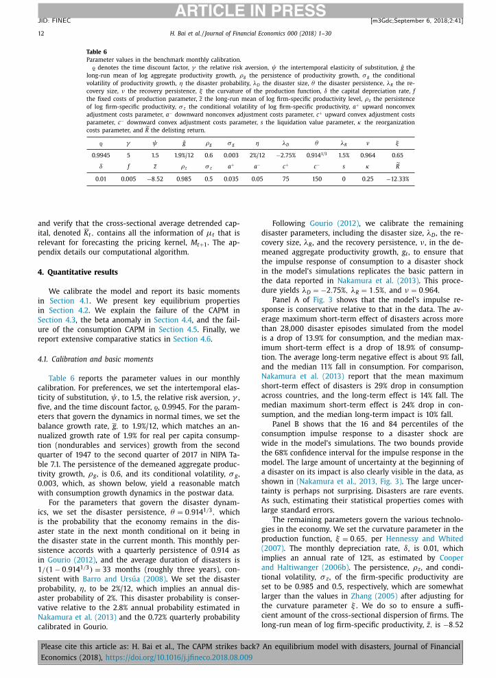
Table 6
Parameter values in the benchmark monthly calibration.
ϱ denotes the time discount factor, γ the relative risk aversion, ψ the intertemporal elasticity of substitution, g the
long-run mean of log aggregate productivity growth, ρg the persistence of productivity growth, σ g the conditional
volatility of productivity growth, η the disaster probability, λD the disaster size, θ the disaster persistence, λR the re-
covery size, ν the recovery persistence, ξ the curvature of the production function, δ the capital depreciation rate, f
the fixed costs of production parameter, z the long-run mean of log firm-specific productivity level, ρz the persistence
of log firm-specific productivity, σ z the conditional volatility of log firm-specific productivity, a + upward nonconvex
adjustment costs parameter, a − downward nonconvex adjustment costs parameter, c + upward convex adjustment costs
parameter, c − downward convex adjustment costs parameter, s the liquidation value parameter, κ the reorganization
costs parameter, and R the delisting return.
ϱ γ ψ g ρg σ g η λD θ λR ν ξ
0.9945 5 1.5 1.9%/12 0.6 0.003 2%/12 −2.75% 0.914 1/3 1.5% 0.964 0.65
δ f z ρz σ z a + a − c + c − s κ ˜ R
0.01 0.005 −8 . 52 0.985 0.5 0.035 0.05 75 150 0 0.25 −12 . 33%
and verify that the cross-sectional average detrended cap-
ital, denoted K t , contains all the information of μt that is
relevant for forecasting the pricing kernel, M t+1 . The ap-
pendix details our computational algorithm.
4. Quantitative results
We calibrate the model and report its basic moments
in Section 4.1 . We present key equilibrium properties
in Section 4.2 . We explain the failure of the CAPM in
Section 4.3 , the beta anomaly in Section 4.4 , and the fail-
ure of the consumption CAPM in Section 4.5 . Finally, we
report extensive comparative statics in Section 4.6 .
4.1. Calibration and basic moments
Table 6 reports the parameter values in our monthly
calibration. For preferences, we set the intertemporal elas-
ticity of substitution, ψ , to 1.5, the relative risk aversion, γ ,
five, and the time discount factor, ϱ, 0.9945. For the param-
eters that govern the dynamics in normal times, we set the
balance growth rate, g , to 1.9%/12, which matches an an-
nualized growth rate of 1.9% for real per capita consump-
tion (nondurables and services) growth from the second
quarter of 1947 to the second quarter of 2017 in NIPA Ta-
ble 7.1. The persistence of the demeaned aggregate produc-
tivity growth, ρg , is 0.6, and its conditional volatility, σ g ,
0.003, which, as shown below, yield a reasonable match
with consumption growth dynamics in the postwar data.
For the parameters that govern the disaster dynam-
ics, we set the disaster persistence, θ = 0 . 914 1 / 3 , which
is the probability that the economy remains in the dis-
aster state in the next month conditional on it being in
the disaster state in the current month. This monthly per-
sistence accords with a quarterly persistence of 0.914 as
in Gourio (2012) , and the average duration of disasters is
1 / (1 − 0 . 914 1 / 3 ) = 33 months (roughly three years), con-
sistent with Barro and Ursúa (2008) . We set the disaster
probability, η, to be 2%/12, which implies an annual dis-
aster probability of 2%. This disaster probability is conser-
vative relative to the 2.8% annual probability estimated in
Nakamura et al. (2013) and the 0.72% quarterly probability
calibrated in Gourio.
Please cite this article as: H. Bai et al., The CAPM strikes back?
Economics (2018), https://doi.org/10.1016/j.jfineco.2018.08.009
Following Gourio (2012) , we calibrate the remaining
disaster parameters, including the disaster size, λD , the re-
covery size, λR , and the recovery persistence, ν , in the de-
meaned aggregate productivity growth, g t , to ensure that
the impulse response of consumption to a disaster shock
in the model’s simulations replicates the basic pattern in
the data reported in Nakamura et al. (2013) . This proce-
dure yields λD = −2 . 75% , λR = 1 . 5% , and ν = 0 . 964 .
Panel A of Fig. 3 shows that the model’s impulse re-
sponse is conservative relative to that in the data. The av-
erage maximum short-term effect of disasters across more
than 28,0 0 0 disaster episodes simulated from the model
is a drop of 13.9% for consumption, and the median max-
imum short-term effect is a drop of 18.9% of consump-
tion. The average long-term negative effect is about 9% fall,
and the median 11% fall in consumption. For comparison,
Nakamura et al. (2013) report that the mean maximum
short-term effect of disasters is 29% drop in consumption
across countries, and the long-term effect is 14% fall. The
median maximum short-term effect is 24% drop in con-
sumption, and the median long-term impact is 10% fall.
Panel B shows that the 16 and 84 percentiles of the
consumption impulse response to a disaster shock are
wide in the model’s simulations. The two bounds provide
the 68% confidence interval for the impulse response in the
model. The large amount of uncertainty at the beginning of
a disaster on its impact is also clearly visible in the data, as
shown in (Nakamura et al., 2013, Fig. 3) . The large uncer-
tainty is perhaps not surprising. Disasters are rare events.
As such, estimating their statistical properties comes with
large standard errors.
The remaining parameters govern the various technolo-
gies in the economy. We set the curvature parameter in the
production function, ξ = 0 . 65 , per Hennessy and Whited
(2007) . The monthly depreciation rate, δ, is 0.01, which
implies an annual rate of 12%, as estimated by Cooper
and Haltiwanger (2006b) . The persistence, ρz , and condi-
tional volatility, σ z , of the firm-specific productivity are
set to be 0.985 and 0.5, respectively, which are somewhat
larger than the values in Zhang (2005) after adjusting for
the curvature parameter ξ . We do so to ensure a suffi-
cient amount of the cross-sectional dispersion of firms. The
long-run mean of log firm-specific productivity, z , is −8 . 52
An equilibrium model with disasters, Journal of Financial

H. Bai et al. / Journal of Financial Economics 0 0 0 (2018) 1–30 13
ARTICLE IN PRESS
JID: FINEC [m3Gdc; September 6, 2018;2:41 ]
0 5 10 15 20 25-0.2
-0.15
-0.1
-0.05
0
0 5 10 15 20 25-0.6
-0.4
-0.2
0
0.2
0.4
Fig. 3. The impulse response of consumption to a disaster shock in the model. In simulated data, when the economy enters the disaster state, we calculate
the cumulative fractional drop in consumption for 25 years after the impulse. The impulse responses are based on more than 28,0 0 0 disaster episodes.
Consumption is time aggregated from the monthly to annual frequency. The blue solid line is the mean impulse response, the black dotted line is the
median, and the two red broken lines in Panel B are the 16 and 84 percentiles in the simulations. (For interpretation of the references to color in this
figure legend, the reader is referred to the web version of this article.)
6 The relatively high frequency of the disaster samples out of 20 0 0 ar-
tificial samples is consistent with the low disaster probability of only 2%
per year. The crux is that we count a (long) sample as a disaster sample if
it contains at least one disaster episode. Roughly, if a disaster occurs with
a probability of p in any given period, the chance of observing no disas-
ters in a given sample is (1 − p) T , in which T is the sample length. The
probability with at least one disaster in the sample is 1 − (1 − p) T . With
to scale the long-run average detrended capital around
unity in simulations.
We set the liquidation value parameter, s = 0 , implying
that shareholders receive nothing in bankruptcy. We set
the reorganizational cost parameter, κ , to 0.25, and the ad-
justment cost parameters a + = 0 . 035 , a − = 0 . 05 , c + = 75 ,
c − = 150 , and the fixed costs parameter, f = 0 . 005 . Be-
cause of the lack of evidence on their values, we calibrate
these parameters to the properties of the book-to-market
deciles and conduct extensive comparative statics to quan-
tify their impact ( Section 4.6 ). Finally, Hou et al. (2017) re-
port that the average delisting return is −12 . 33% in the
Center for Research in Security Prices (CRSP) database. Ac-
cordingly, we set the delisting return in the model, ˜ R , to
the same value.
Table 7 reports the basic moments of aggregate out-
put, consumption, and investment growth rates both in the
data and in the model. Output in the data is per capita
gross domestic product in chained dollars from NIPA Table
7.1. Consumption is per capita consumption expenditures
on nondurables plus services in chained dollars from NIPA
Table 7.1. Investment is real nonresidential gross private,
fixed domestic investment from NIPA Table 1.1.3, scaled
by population series from NIPA Table 7.1. The data sam-
ple with disasters is annual from 1930 to 2016, and the
data sample without disasters is quarterly from the second
quarter of 1947 to that of 2017.
To calculate the model moments, we simulate 20 0 0 ar-
tificial samples, each with 30,0 0 0 firms and 20 0 0 months.
Because we need to compute consumption moments, we
simulate a large number of firms, 30,0 0 0, which is nec-
essary to ensure convergence in the laws of motion in
the Krusell–Smith algorithm ( Appendix A.2 ). We start
each simulation by setting the initial capital stocks of all
firms to unity and the initial log firm-specific productiv-
ity levels to its long-run mean, z . We drop the first 944
Please cite this article as: H. Bai et al., The CAPM strikes back?
Economics (2018), https://doi.org/10.1016/j.jfineco.2018.08.009
months to neutralize the impact of the initial condition.
The remaining 1056 months of simulated data are treated
as from the model’s stationary distribution. The sample
size is comparable with the annual sample from 1929
to 2016 for output, consumption, and investment in the
data.
When at least one disaster is realized in an artificial
sample, we time aggregate the 1056 months into 88 an-
nual observations. Time aggregation means that we add up
12 months within a given year, and treat the sum as the
year’s observation. On artificial samples with no disasters,
we time aggregate the initial 846 months into 282 quar-
ters to be comparable with the quarterly sample from the
first quarter of 1947 to the second quarter of 2017 in the
data. Out of the 20 0 0 artificial samples, 1688 have at least
one disaster, and the remaining 312 have none. As such,
the frequency of having 1056 months (88 years) with at
least one disaster episode is 1688 / 20 0 0 = 84 . 4% . 6
From Panel A of Table 7 , the output volatility in the
model is close to that in the data, 4.41% versus 4.79% per
annum, with disasters, but lower, 0.5% versus 0.94% per
quarter, without disasters. The first-order autocorrelation
of output growth is somewhat higher in the model than
that in the data, 0.69 versus 0.54, with disasters, and 0.43
versus 0.37, without disasters. The autocorrelations turn
negative at the four- and five-year horizons in the data, but
remain positive in the model.
our monthly calibration, this probability is 1 − (1 − 0 . 02 / 12) 1 , 056 = 82 . 8% .
An equilibrium model with disasters, Journal of Financial

14 H. Bai et al. / Journal of Financial Economics 0 0 0 (2018) 1–30
ARTICLE IN PRESS
JID: FINEC [m3Gdc; September 6, 2018;2:41 ]
Table 7
Basic moments of log output, consumption, and investment growth.
The data moments in samples with disasters are based on the annual sample from 1930 to 2016 (87 years), and those in samples without disasters
on the quarterly sample from the second quarter of 1947 to the second quarter of 2017 (281 quarters). “Vol” denotes volatility, “Skew” skewness, and
“Kurt” kurtosis. The volatilities in samples with disasters are in annual percent and the volatilities in samples without disasters in quarterly percent. Ar i is the i th-order autocorrelation. Output in the data is per capita gross domestic product in chained dollars from NIPA Table 7.1, consumption per capita
consumption expenditures on nondurables plus services in chained dollars from NIPA Table 7.1, and investment real nonresidential gross private, fixed
domestic investment from NIPA Table 1.1.3, scaled by population series from NIPA Table 7.1. The model moments in the columns denoted “mean” are
averaged across 20 0 0 samples, each with 30,0 0 0 firms and 20 0 0 months. Columns denoted “2.5,” “50,” and “97.5” report 2.5, 50, and 97.5 percentiles
across the simulations. The p -value ( p ) is the percentage with which a model moment is larger than its data counterpart.
Samples with disasters, annual Samples without disasters, quarterly
Data Mean 2.5 50 97.5 p Data Mean 2.5 50 97.5 p
Panel A: Output growth
Vol 4.79 4.41 1.37 4.26 8.50 0.41 0.94 0.50 0.44 0.49 0.65 0.00
Skew −0.29 −1.89 −4.32 −2.09 2.07 0.15 −0.18 0.02 −0.32 −0.02 1.02 0.88
Kurt 6.14 11.43 2.95 9.54 27.52 0.78 4.51 3.05 2.41 2.90 5.11 0.04
Ar 1 0.54 0.69 0.27 0.73 0.93 0.80 Ar 1 0.37 0.43 0.30 0.42 0.63 0.82
Ar 2 0.19 0.38 −0.15 0.40 0.82 0.74 Ar 4 −0.07 0.11 −0.06 0.09 0.35 0.99
Ar 3 −0.14 0.23 −0.22 0.21 0.72 0.92 Ar 8 −0.02 0.07 −0.09 0.06 0.26 0.82
Ar 4 −0.34 0.14 −0.26 0.12 0.62 0.99 Ar 12 −0.12 0.05 −0.10 0.04 0.24 0.99
Ar 5 −0.19 0.09 −0.25 0.07 0.53 0.94 Ar 20 0.05 0.02 −0.13 0.02 0.19 0.35
Panel B: Consumption growth
Vol 2.13 4.28 1.30 4.13 8.28 0.87 0.50 0.46 0.40 0.45 0.60 0.09
Skew −1.48 −1.93 −4.42 −2.14 2.13 0.32 −0.41 0.02 −0.31 −0.03 1.14 0.99
Kurt 8.09 11.66 2.98 9.63 28.82 0.63 4.17 3.10 2.44 2.93 5.83 0.04
Ar 1 0.48 0.69 0.24 0.74 0.93 0.85 Ar 1 0.31 0.44 0.31 0.44 0.66 0.97
Ar 2 0.18 0.39 −0.15 0.42 0.83 0.75 Ar 4 0.10 0.13 −0.05 0.12 0.39 0.61
Ar 3 −0.05 0.24 −0.22 0.23 0.72 0.86 Ar 8 −0.02 0.08 −0.08 0.08 0.30 0.86
Ar 4 −0.19 0.16 −0.24 0.13 0.63 0.95 Ar 12 0.08 0.06 −0.10 0.05 0.28 0.35
Ar 5 0.00 0.10 −0.24 0.08 0.55 0.70 Ar 20 −0.04 0.03 −0.13 0.03 0.21 0.83
Panel C: Investment growth
Vol 13.53 19.56 3.10 12.28 71.84 0.45 2.40 1.09 0.98 1.08 1.33 0.00
Skew −1.33 −0.17 0.02 −1.56 2.69 0.68 −0.53 −0.20 −0.58 −0.20 0.25 0.96
Kurt 7.07 27.45 6.68 19.50 100.98 0.96 4.73 3.70 2.85 3.41 5.26 0.03
Ar 1 0.41 0.18 0.00 0.23 0.59 0.17 Ar 1 0.46 0.24 0.11 0.24 0.38 0.01
Ar 2 −0.15 −0.06 0.00 0.00 −0.44 0.71 Ar 4 −0.03 −0.00 −0.12 −0.01 0.14 0.63
Ar 3 −0.33 −0.07 0.00 0.00 0.38 0.96 Ar 8 −0.18 −0.01 −0.12 −0.01 0.11 1.00
Ar 4 −0.17 −0.06 −0.00 0.00 −0.07 0.84 Ar 12 −0.09 −0.01 −0.13 −0.01 0.11 0.90
Ar 5 −0.05 −0.05 −0.00 −0.05 −0.06 0.57 Ar 20 0.03 −0.00 −0.12 0.00 0.11 0.29
Panel B shows that the consumption volatility in the
model is close to that in the data, 0.46% versus 0.5% per
quarter, without disasters, but higher, 4.28% versus 2.13%
per annum, with disasters. The consumption growth is
negatively skewed and fat tailed both in the data and in
the model, with disasters. Without disasters, the autocor-
relation structure of the consumption growth in the model
resembles that in the data. Except for the first-quarter au-
tocorrelation, which is somewhat higher in the model than
in the data, 0.44 versus 0.31, none of the p -values at longer
lags indicate incompatibility between the data and model
autocorrelations. With disasters, the autocorrelations are
somewhat higher in the model than in the data, but none
of the p -values indicate incompatibility.
Finally, Panel C shows that the investment volatility in
the model is higher than that in the data, 19.6% versus
13.5% per annum, with disasters, but lower, 1.1% versus
2.4% per quarter, without disasters. The aggregate invest-
ment growth is more autocorrelated in the data than in
the model. The first-lag autocorrelation is 0.41 in the long
annual sample but only 0.18 in the model’s disaster sam-
ples. The first-lag autocorrelation is 0.46 in the short quar-
terly sample in the data but 0.24 in the model’s samples
without disasters. Investment growth is negatively autocor-
Please cite this article as: H. Bai et al., The CAPM strikes back?
Economics (2018), https://doi.org/10.1016/j.jfineco.2018.08.009
related at longer lags in annual samples with disasters but
largely uncorrelated in quarterly samples without disasters.
For aggregate asset pricing moments, it is customary in
the disaster literature to match international data ( Barro,
2006 ). In particular, Petrosky-Nadeau et al. (2018) com-
pile a historical cross-country panel of real stock market
returns and real interest rates by drawing from Global Fi-
nancial Data and an updated Dimson et al. (2002) dataset
obtained from Morningstar. Petrosky-Nadeau et al.
(2018) report that the equity premium is, on average,
6.6% per annum across countries, ranging from 3.66% in
the United Kingdom to 9.66% in Japan. The real interest
rate is, on average, 1%, ranging from −2 . 44% in Austria to
3.5% in Denmark. The stock market volatility is, on average,
25.6%, and the real interest rate volatility 12.32%. The high
interest rate volatility in the historical data is mostly due
to sovereign default, which is abstracted from our model.
In simulations, our model implies an average equity
premium of 9.6%, with a 95% confidence interval of (8.5%,
10.2%), and an average interest rate of 2.6%, with a confi-
dence interval of (0.15%, 4.15%). The interest rate volatility
is 0.8%, as the intertemporal elasticity of substitution, ψ , is
1.5. More important, the stock market volatility is only 7.7%
in the model. This lower volatility than that in the data
An equilibrium model with disasters, Journal of Financial

H. Bai et al. / Journal of Financial Economics 0 0 0 (2018) 1–30 15
ARTICLE IN PRESS
JID: FINEC [m3Gdc; September 6, 2018;2:41 ]
-0.540
0
0
0.5
1
Detrended capital
20
Log firm-specific productivity
1.5
-10
0 -20
-0.540
0
0
0.5
1
Detrended capital
20
Log firm-specific productivity
1.5
-10
0 -20
Panel A: Iit/ Kit in the disaster state Panel B: The difference in Iit/ Kit betweenthe mean normal state and disaster state
Fig. 4. Optimal policy functions in the model. Based on the model’s competitive equilibrium, Panel A plots the investment-to-capital ratio, I it / K it , on the K it - z it - g t - K t grid when the demeaned aggregate productivity growth, g t , is set to be the disaster size, λD . K it is the detrended firm-level capital, z it log firm-
specific productivity, and K t the cross-sectional average detrended capital (which is set to be the median of its grid). Panel B plots the investment-to-capital
ratio when g t is set to be zero (the mean normal state) minus the investment-to-capital ratio in the disaster state.
is in line with Barro (20 06, 20 09) . Introducing the time-
varying disaster probability per Gourio (2012) and Wachter
(2013) can fix this weakness. Alas, doing so would add one
more state and increase the computational burden expo-
nentially. More important, introducing an extra aggregate
state will most likely strengthen the model’s ability to ex-
plain the failure of the CAPM, which is our main focus. We
opt to achieve this goal with a more parsimonious model.
4.2. Key properties of the competitive equilibrium
Before we present detailed quantitative results on the
cross-section, we characterize key equilibrium properties
by presenting key variables on the numerical grid and
across the book-to-market deciles.
4.2.1. Optimal policy functions
Fig. 4 uses the model’s solution on the K it - z it - g t - K t
grid to plot the optimal investment-to-capital ratio, I it / K it ,
against the detrended capital, K it , and the log firm-specific
productivity, z it . Panel A makes the plot in the disaster
state, with the demeaned aggregate productivity growth,
g t , set to the disaster size, λD . To examine the impact of
disasters, Panel B plots the difference between
I it / K it , when
g t = 0 (the mean of normal states), and
I it / K it when g t =
λD . In both panels, the cross-sectional average detrended
capital, K t , is set to be the median on its grid.
Panel A shows that the optimal investment-to-capital
ratio, I it / K it , rises with firms-specific productivity. Intu-
itively, more productive firms have higher shadow value
of capital and consequently invest more. In addition, I it / K it
decreases with capital. This pattern is a result of decreas-
ing returns to scale in the production function in Eq. (5) .
In Panel A, only a portion of the K it - z it grid is plotted.
The missing region is exactly where firms exit the econ-
omy. Naturally, firms with low firm-specific productivity
are more likely to exit than firms with high firm-specific
Please cite this article as: H. Bai et al., The CAPM strikes back?
Economics (2018), https://doi.org/10.1016/j.jfineco.2018.08.009
productivity. In addition, because the fixed costs of pro-
duction are proportional to capital, firms with more cap-
ital have to pay higher costs than firms with less capital to
stay in production. As such, high- K firms are more likely to
exit than low- K firms.
Panel B shows that the disaster risk affects the invest-
ment policy the most for firms that are close to the exit
boundary. For these firms, the differences in the optimal
investment-to-capital ratio between the mean normal state
and the disaster state are most visible.
4.2.2. Risk and risk premiums
Fig. 5 plots the true beta, βM
it , and the expected risk
premium, E t [ R it+1 ] − r f t , against the detrended capital, K it ,
and the log firm-specific productivity, z it , for two values of
the detrended aggregate productivity growth, g t , the disas-
ter state, λD , and the mean normal state (zero). The cross-
sectional average detrended capital, K t , is again set to be
the median of its grid.
Panel A shows that in the disaster state, firms that are
close to the exit boundary, such as low- z firms, are sub-
stantially riskier than firms that are far away from the exit
boundary, such as high- z firms. Accordingly, Panel C shows
that low- z firms earn substantially higher risk premiums
than high- z firms in the disaster state. In sharp contrast,
Panels B and D show that risk and risk premiums are
largely flat across firms in the mean normal state.
Intuitively, the economic mechanism is similar qual-
itatively to, but turbocharged quantitatively relative to,
the asymmetry mechanism in Zhang (2005) . Because of
asymmetric adjustment costs, low- z firms are burdened
with more unproductive capital, finding it more difficult to
downsize than high- z firms. As such, low- z firms are riskier
than high- z firms in disasters. In contrast, in normal times,
even low- z firms do not have strong incentives to disinvest.
As such, the asymmetry mechanism fails to take strong ef-
fect, giving rise to weak spreads in risk and risk premiums
An equilibrium model with disasters, Journal of Financial

16 H. Bai et al. / Journal of Financial Economics 0 0 0 (2018) 1–30
ARTICLE IN PRESS
JID: FINEC [m3Gdc; September 6, 2018;2:41 ]
040
10
0
20
Detrended capital
20
Log firm-specific productivity
30
-10
0 -20
040
10
0
20
Detrended capital
20
Log firm-specific productivity
30
-10
0 -20
040
0
0.5
Detrended capital
20
Log firm-specific productivity
1
-10
0 -20
040
0
0.5
Detrended capital
20
Log firm-specific productivity
1
-10
0 -20
Panel A: True beta, βMit , the disaster state Panel B: True beta, βM
it , the mean normalstate
Panel C: Expected risk premium,Et[Rit+1] − rft, the disaster state
Panel D: Expected risk premium,Et[Rit+1] − rft, the mean normal state
Fig. 5. Disaster risk and risk premiums in the model. This figure plots the true beta, βM it
, and the expected risk premium, E t [ R it+1 ] − r f t , on the K it - z it - g t - K t grid. K it is the detrended firm-level capital, z it log firm-specific productivity, g t the demeaned aggregate productivity growth, and K t the cross-sectional
average detrended capital. We set g t to be the disaster size, λD , in Panels A and C and set g t to be zero, which is the mean of the normal states, in Panels
B and D. K t is set to be the median of its grid in all panels.
across firms. While Zhang describes the working of this
mechanism in recessions, we turbocharge it in disasters.
This asymmetry mechanism is related to our modeling
of disasters as large drops in the aggregate productivity
growth. Besides productivity disasters, Gourio (2012) also
models disasters via capital destruction, which would seem
to weaken the asymmetry mechanism in Fig. 5 . However,
while capital destruction is realistic for wars, it is less obvi-
ous for economic disasters. Because we aim to explain the
stylized facts that feature the Great Depression, which is
an economic disaster, we opt not to model capital destruc-
tion. More important, Gourio motivates capital destruction
in disasters as large negative shocks on the “quality” of
capital: “Perhaps it is not the physical capital but the in-
tangible capital (customer and employee value) that is de-
stroyed during prolonged economic depressions (p. 2740).”
The accumulation of a large quantity of capital with dete-
riorating quality in disasters likely strengthens the asym-
metry mechanism.
Please cite this article as: H. Bai et al., The CAPM strikes back?
Economics (2018), https://doi.org/10.1016/j.jfineco.2018.08.009
4.2.3. Value versus growth
To shed light on the key properties of the book-to-
market deciles, we simulate 20 0 0 artificial samples, each
with 50 0 0 firms and 20 0 0 months. We start each simu-
lation by setting the initial capital stocks of all firms at
unity and the initial log firm-specific productivity to its
long-run mean, z . We drop the first 908 months to neu-
tralize the impact of the initial condition and treat the re-
maining 1092 months as from the economy’s stationary
distribution. The sample size is comparable to the period
from July 1926 to June 2017 in the data. We calculate the
model moments on each artificial sample and report cross-
simulation averaged results. To demonstrate the impact of
disasters, we calculate cross-simulation averages separately
on samples with and without disasters.
Fig. 6 reports the results. From Panel A, value firms
with high book-to-market have about 4.5 times more cap-
ital than growth firms with low book-to-market. All firms
have slightly more capital in the disaster samples than in
An equilibrium model with disasters, Journal of Financial
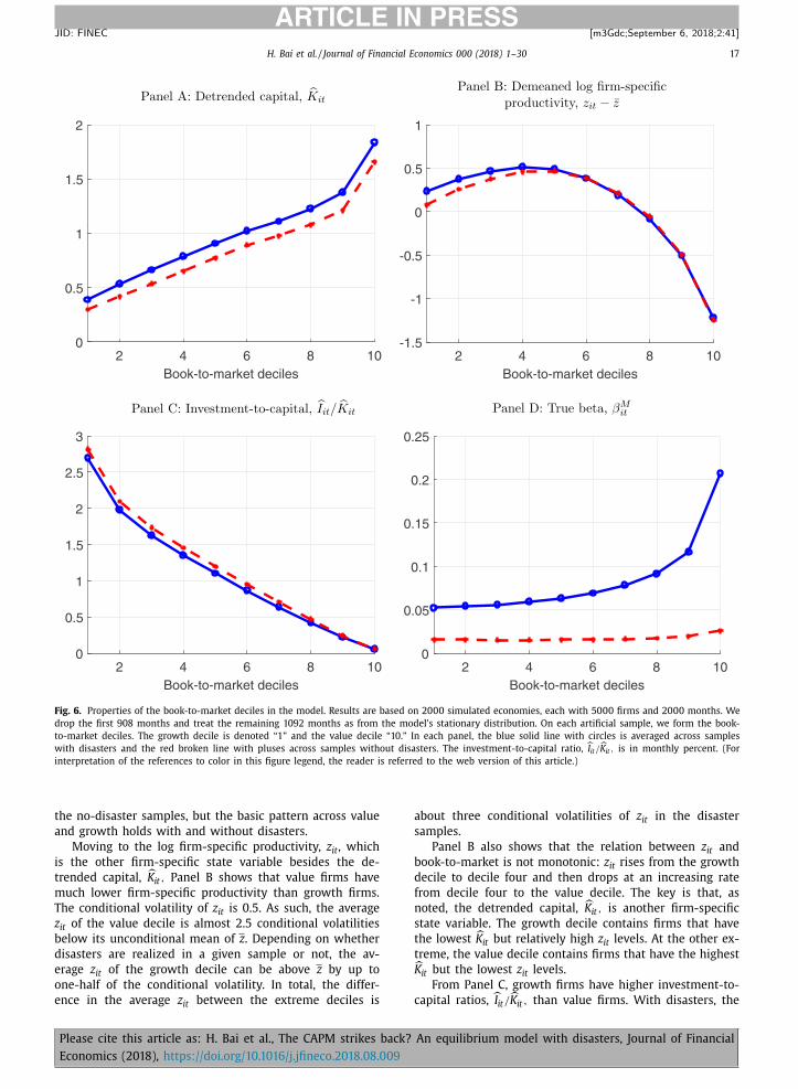
H. Bai et al. / Journal of Financial Economics 0 0 0 (2018) 1–30 17
ARTICLE IN PRESS
JID: FINEC [m3Gdc; September 6, 2018;2:41 ]
2 4 6 8 10Book-to-market deciles
0
0.5
1
1.5
2
2 4 6 8 10Book-to-market deciles
-1.5
-1
-0.5
0
0.5
1
2 4 6 8 10Book-to-market deciles
0
0.5
1
1.5
2
2.5
3
2 4 6 8 10Book-to-market deciles
0
0.05
0.1
0.15
0.2
0.25
Panel A: Detrended capital, KitPanel B: Demeaned log firm-specific
productivity, zit − z
Panel C: Investment-to-capital, Iit/ Kit Panel D: True beta, βMit
Fig. 6. Properties of the book-to-market deciles in the model. Results are based on 20 0 0 simulated economies, each with 50 0 0 firms and 20 0 0 months. We
drop the first 908 months and treat the remaining 1092 months as from the model’s stationary distribution. On each artificial sample, we form the book-
to-market deciles. The growth decile is denoted “1” and the value decile “10.” In each panel, the blue solid line with circles is averaged across samples
with disasters and the red broken line with pluses across samples without disasters. The investment-to-capital ratio, I it / K it , is in monthly percent. (For
interpretation of the references to color in this figure legend, the reader is referred to the web version of this article.)
the no-disaster samples, but the basic pattern across value
and growth holds with and without disasters.
Moving to the log firm-specific productivity, z it , which
is the other firm-specific state variable besides the de-
trended capital, K it , Panel B shows that value firms have
much lower firm-specific productivity than growth firms.
The conditional volatility of z it is 0.5. As such, the average
z it of the value decile is almost 2.5 conditional volatilities
below its unconditional mean of z . Depending on whether
disasters are realized in a given sample or not, the av-
erage z it of the growth decile can be above z by up to
one-half of the conditional volatility. In total, the differ-
ence in the average z it between the extreme deciles is
Please cite this article as: H. Bai et al., The CAPM strikes back?
Economics (2018), https://doi.org/10.1016/j.jfineco.2018.08.009
about three conditional volatilities of z it in the disaster
samples.
Panel B also shows that the relation between z it and
book-to-market is not monotonic: z it rises from the growth
decile to decile four and then drops at an increasing rate
from decile four to the value decile. The key is that, as
noted, the detrended capital, K it , is another firm-specific
state variable. The growth decile contains firms that have
the lowest K it but relatively high z it levels. At the other ex-
treme, the value decile contains firms that have the highest K it but the lowest z it levels.
From Panel C, growth firms have higher investment-to-
capital ratios, I it / K it , than value firms. With disasters, the
An equilibrium model with disasters, Journal of Financial
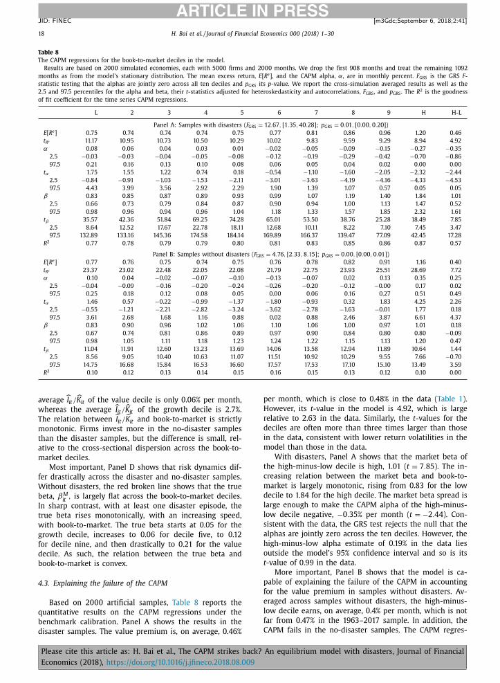
18 H. Bai et al. / Journal of Financial Economics 0 0 0 (2018) 1–30
ARTICLE IN PRESS
JID: FINEC [m3Gdc; September 6, 2018;2:41 ]
Table 8
The CAPM regressions for the book-to-market deciles in the model.
Results are based on 20 0 0 simulated economies, each with 50 0 0 firms and 20 0 0 months. We drop the first 908 months and treat the remaining 1092
months as from the model’s stationary distribution. The mean excess return, E [ R e ], and the CAPM alpha, α, are in monthly percent. F GRS is the GRS F -
statistic testing that the alphas are jointly zero across all ten deciles and p GRS its p -value. We report the cross-simulation averaged results as well as the
2.5 and 97.5 percentiles for the alpha and beta, their t -statistics adjusted for heteroskedasticity and autocorrelations, F GRS , and p GRS . The R 2 is the goodness
of fit coefficient for the time series CAPM regressions.
L 2 3 4 5 6 7 8 9 H H-L
Panel A: Samples with disasters ( F GRS = 12 . 67 , [1 . 35 , 40 . 28] ; p GRS = 0 . 01 , [0 . 00 , 0 . 20] )
E [ R e ] 0.75 0.74 0.74 0.74 0.75 0.77 0.81 0.86 0.96 1.20 0.46
t R e 11.17 10.95 10.73 10.50 10.29 10.02 9.83 9.59 9.29 8.94 4.92
α 0.08 0.06 0.04 0.03 0.01 −0.02 −0.05 −0.09 −0.15 −0.27 −0.35
2.5 −0.03 −0.03 −0.04 −0.05 −0.08 −0.12 −0.19 −0.29 −0.42 −0.70 −0.86
97.5 0.21 0.16 0.13 0.10 0.08 0.06 0.05 0.04 0.02 0.00 0.00
t α 1.75 1.55 1.22 0.74 0.18 −0.54 −1.10 −1.60 −2.05 −2.32 −2.44
2.5 −0.84 −0.91 −1.03 −1.53 −2.11 −3.01 −3.63 −4.19 −4.16 −4.33 −4.53
97.5 4.43 3.99 3.56 2.92 2.29 1.90 1.39 1.07 0.57 0.05 0.05
β 0.83 0.85 0.87 0.89 0.93 0.99 1.07 1.19 1.40 1.84 1.01
2.5 0.66 0.73 0.79 0.84 0.87 0.90 0.94 1.00 1.13 1.47 0.52
97.5 0.98 0.96 0.94 0.96 1.04 1.18 1.33 1.57 1.85 2.32 1.61
t β 35.57 42.36 51.84 69.25 74.28 65.01 53.50 38.76 25.28 18.49 7.85
2.5 8.64 12.52 17.67 22.78 18.11 12.68 10.11 8.22 7.10 7.45 3.47
97.5 132.89 133.16 145.36 174.58 184.14 169.89 166.37 139.47 77.09 42.45 17.28
R 2 0.77 0.78 0.79 0.79 0.80 0.81 0.83 0.85 0.86 0.87 0.57
Panel B: Samples without disasters ( F GRS = 4 . 76 , [2 . 33 , 8 . 15] ; p GRS = 0 . 00 , [0 . 00 , 0 . 01] )
E [ R e ] 0.77 0.76 0.75 0.74 0.75 0.76 0.78 0.82 0.91 1.16 0.40
t R e 23.37 23.02 22.48 22.05 22.08 21.79 22.75 23.93 25.51 28.69 7.72
α 0.10 0.04 −0.02 −0.07 −0.10 −0.13 −0.07 0.02 0.13 0.35 0.25
2.5 −0.04 −0.09 −0.16 −0.20 −0.24 −0.26 −0.20 −0.12 −0.00 0.17 0.02
97.5 0.25 0.18 0.12 0.08 0.05 0.00 0.06 0.16 0.27 0.51 0.49
t α 1.46 0.57 −0.22 −0.99 −1.37 −1.80 −0.93 0.32 1.83 4.25 2.26
2.5 −0.55 −1.21 −2.21 −2.82 −3.24 −3.62 −2.78 −1.63 −0.01 1.77 0.18
97.5 3.61 2.68 1.68 1.16 0.88 0.02 0.88 2.46 3.87 6.61 4.37
β 0.83 0.90 0.96 1.02 1.06 1.10 1.06 1.00 0.97 1.01 0.18
2.5 0.67 0.74 0.81 0.86 0.89 0.97 0.90 0.84 0.80 0.80 −0.09
97.5 0.98 1.05 1.11 1.18 1.23 1.24 1.22 1.15 1.13 1.20 0.47
t β 11.04 11.91 12.60 13.23 13.69 14.06 13.58 12.94 11.89 10.64 1.44
2.5 8.56 9.05 10.40 10.63 11.07 11.51 10.92 10.29 9.55 7.66 −0.70
97.5 14.75 16.68 15.84 16.53 16.60 17.57 17.53 17.10 15.10 13.49 3.59
R 2 0.10 0.12 0.13 0.14 0.15 0.16 0.15 0.13 0.12 0.10 0.00
average I it / K it of the value decile is only 0.06% per month,
whereas the average I it / K it of the growth decile is 2.7%.
The relation between
I it / K it and book-to-market is strictly
monotonic. Firms invest more in the no-disaster samples
than the disaster samples, but the difference is small, rel-
ative to the cross-sectional dispersion across the book-to-
market deciles.
Most important, Panel D shows that risk dynamics dif-
fer drastically across the disaster and no-disaster samples.
Without disasters, the red broken line shows that the true
beta, βM
it , is largely flat across the book-to-market deciles.
In sharp contrast, with at least one disaster episode, the
true beta rises monotonically, with an increasing speed,
with book-to-market. The true beta starts at 0.05 for the
growth decile, increases to 0.06 for decile five, to 0.12
for decile nine, and then drastically to 0.21 for the value
decile. As such, the relation between the true beta and
book-to-market is convex.
4.3. Explaining the failure of the CAPM
Based on 20 0 0 artificial samples, Table 8 reports the
quantitative results on the CAPM regressions under the
benchmark calibration. Panel A shows the results in the
disaster samples. The value premium is, on average, 0.46%
Please cite this article as: H. Bai et al., The CAPM strikes back?
Economics (2018), https://doi.org/10.1016/j.jfineco.2018.08.009
per month, which is close to 0.48% in the data ( Table 1 ).
However, its t -value in the model is 4.92, which is large
relative to 2.63 in the data. Similarly, the t -values for the
deciles are often more than three times larger than those
in the data, consistent with lower return volatilities in the
model than those in the data.
With disasters, Panel A shows that the market beta of
the high-minus-low decile is high, 1.01 ( t = 7 . 85 ). The in-
creasing relation between the market beta and book-to-
market is largely monotonic, rising from 0.83 for the low
decile to 1.84 for the high decile. The market beta spread is
large enough to make the CAPM alpha of the high-minus-
low decile negative, −0 . 35% per month ( t = −2 . 44 ). Con-
sistent with the data, the GRS test rejects the null that the
alphas are jointly zero across the ten deciles. However, the
high-minus-low alpha estimate of 0.19% in the data lies
outside the model’s 95% confidence interval and so is its
t -value of 0.99 in the data.
More important, Panel B shows that the model is ca-
pable of explaining the failure of the CAPM in accounting
for the value premium in samples without disasters. Av-
eraged across samples without disasters, the high-minus-
low decile earns, on average, 0.4% per month, which is not
far from 0.47% in the 1963–2017 sample. In addition, the
CAPM fails in the no-disaster samples. The CAPM regres-
An equilibrium model with disasters, Journal of Financial

H. Bai et al. / Journal of Financial Economics 0 0 0 (2018) 1–30 19
ARTICLE IN PRESS
JID: FINEC [m3Gdc; September 6, 2018;2:41 ]
Fig. 7. The CAPM regressions of the value premium in the model. The value premium is the value-minus-growth decile return. The market excess return
is the market portfolio return value-weighted from all the firms minus the interest rate. Based on 20 0 0 simulations from the model, this figure reports
the scatter plot and the fitted line from regressing the value premium on the market excess return. The fitted line in Panel A is estimated by stacking the
monthly observations from all the samples with disasters and the fitted line in Panel B from all the samples without disasters. Both the value premium
and market excess return are in monthly percent.
7 The scatter plot in Panel A of Fig. 7 shows three large blocks, with
the left, middle, and right blocks from disasters, normal times, and re-
coveries, respectively. The discreteness arises because we simulate from
the discrete Markov chain with the transition probabilities in Eq. (13) . If
we use a sufficiently large number of grid points for the normal states
and also simulate the economy for a sufficiently long period to ensure re-
mote grid points are visited, the discreteness would disappear. However,
because the persistence in the aggregate demeaned productivity growth,
ρg , is relatively low, 0.6, a five-point grid is sufficient to ensure accuracy
for simulated moments.
sion of the high-minus-low decile yields an alpha of 0.25%
( t = 2 . 26 ). The 95% confidence interval for the alpha spans
from 0.02% to 0.49%, and the interval for its t -value from
0.18 to 4.37. As such, the alpha estimate of 0.43% ( t = 1 . 89 )
in the data lies well within the model’s distribution. Also,
the market beta for the high-minus-low decile is small,
0.18 ( t = 1 . 44 ), which is not far from 0.07 ( t = 0 . 86 ) in the
data ( Table 1 ). The R 2 is in effect zero. Finally, again con-
sistent with data, the GRS test rejects that the alphas are
jointly zero across the ten deciles.
4.3.1. Nonlinearity in the CAPM regressions
To shed light on the driving force behind our key re-
sults in Table 8, Fig. 7 reports the scatter plots of the CAPM
regressions of the value-minus-growth decile in the model.
Panel A is the scatter plot from stacking the disaster sam-
ples underlying Panel A in Table 8 , and Panel B the scat-
ter plot from stacking the no-disaster samples underlying
Panel B in Table 8 .
The basic pattern in Fig. 7 resembles Fig. 1 in the
US sample. From Panel A of Fig. 7 , the value-minus-
growth return covaries strongly with the market excess
return in the disaster samples. Both returns are large
and negative in disasters but large and positive in the
subsequent recoveries. As a result, the market beta for the
value-minus-growth decile is 1.06, which is a population
moment because of the large number of simulations.
However, the CAPM alpha is −0 . 39% per month, implying
that the unconditional CAPM does not hold in our dynamic
single-factor model. In contrast, Panel B shows that the
value-minus-growth return does not covary much with the
market excess return in the no-disaster samples. Without
the large swings in the same direction in the value-minus-
growth return and market excess return during disasters
and subsequent recoveries, the CAPM regression line is
largely flat, resembling the 1963–2017 US evidence ( Fig. 1 ).
Please cite this article as: H. Bai et al., The CAPM strikes back?
Economics (2018), https://doi.org/10.1016/j.jfineco.2018.08.009
The market beta is only 0.18, and the CAPM alpha is 0.25%
per month. 7
4.3.2. Nonlinearity in the pricing kernel
The disaster risk induces strong nonlinearity in the
pricing kernel, making the CAPM a poor proxy of the pric-
ing kernel. If the CAPM holds exactly, the pricing kernel
can be expressed as a linear function of the market ex-
cess return, R Mt+1 , i.e., M t+1 = l 0 + l 1 R Mt+1 , in which l 0 and
l 1 are constants ( Cochrane, 2005b ). Fig. 8 shows that the
pricing kernel in the model is far from a linear function of
the market excess return. Panel A reports the scatter plot
for regressing the pricing kernel on the market excess re-
turn based on the disaster samples. The regression yields
an intercept of 1.22, a slope of −0 . 14 , but an R 2 of only
21%, despite the model’s single-factor structure. The linear
CAPM fits poorly the observations from the disaster state,
with high realizations of the pricing kernel, and the ob-
servations from the recovery state, with low realizations
of the pricing kernel. From Panel B, the CAPM is an even
worse proxy for the pricing kernel in the no-disaster sam-
ples. The regression slope is only −0 . 03 , although the R 2 is
23% (because of missing large outliers). As such, the CAPM
fails badly in the no-disaster samples.
An equilibrium model with disasters, Journal of Financial
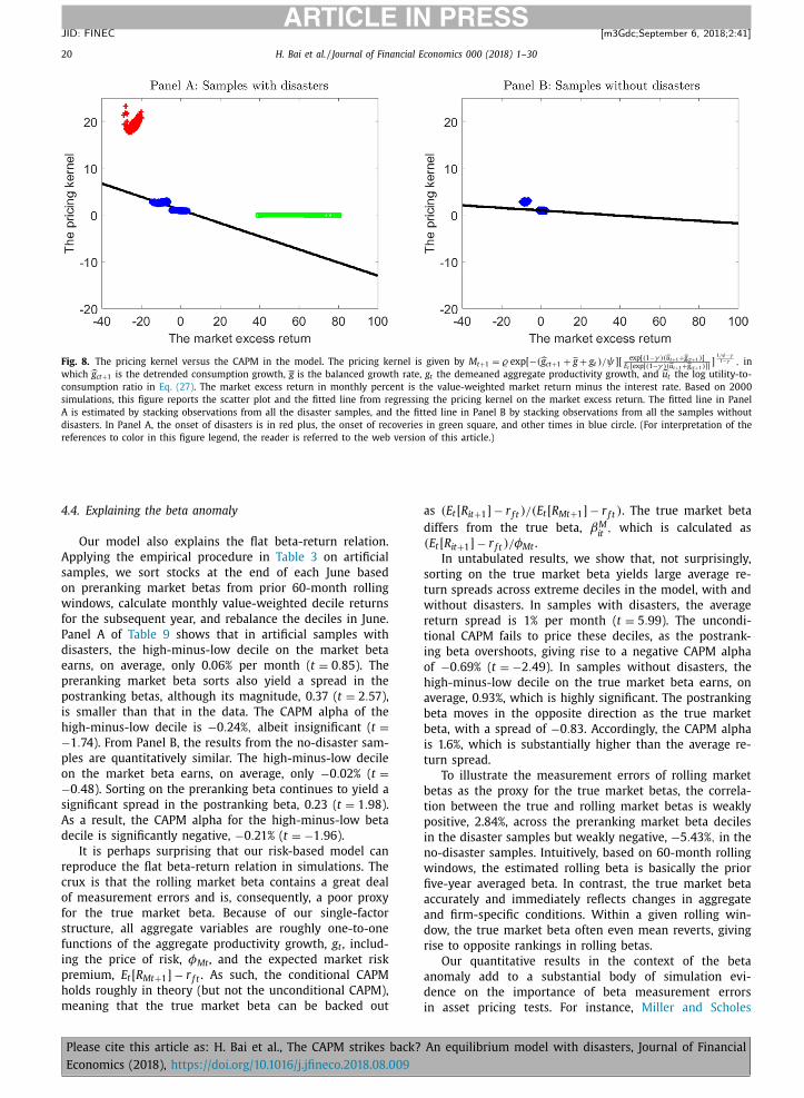
20 H. Bai et al. / Journal of Financial Economics 0 0 0 (2018) 1–30
ARTICLE IN PRESS
JID: FINEC [m3Gdc; September 6, 2018;2:41 ]
Fig. 8. The pricing kernel versus the CAPM in the model. The pricing kernel is given by M t+1 = � exp [ −( g ct+1 + g + g t ) /ψ][ exp [(1 −γ )( u t+1 + g ct+1 )] E t [ exp [(1 −γ )( u t+1 + g ct+1 )]]
] 1 /ψ−γ
1 −γ , in
which g ct+1 is the detrended consumption growth, g is the balanced growth rate, g t the demeaned aggregate productivity growth, and u t the log utility-to-
consumption ratio in Eq. (27) . The market excess return in monthly percent is the value-weighted market return minus the interest rate. Based on 20 0 0
simulations, this figure reports the scatter plot and the fitted line from regressing the pricing kernel on the market excess return. The fitted line in Panel
A is estimated by stacking observations from all the disaster samples, and the fitted line in Panel B by stacking observations from all the samples without
disasters. In Panel A, the onset of disasters is in red plus, the onset of recoveries in green square, and other times in blue circle. (For interpretation of the
references to color in this figure legend, the reader is referred to the web version of this article.)
4.4. Explaining the beta anomaly
Our model also explains the flat beta-return relation.
Applying the empirical procedure in Table 3 on artificial
samples, we sort stocks at the end of each June based
on preranking market betas from prior 60-month rolling
windows, calculate monthly value-weighted decile returns
for the subsequent year, and rebalance the deciles in June.
Panel A of Table 9 shows that in artificial samples with
disasters, the high-minus-low decile on the market beta
earns, on average, only 0.06% per month ( t = 0 . 85 ). The
preranking market beta sorts also yield a spread in the
postranking betas, although its magnitude, 0.37 ( t = 2 . 57 ),
is smaller than that in the data. The CAPM alpha of the
high-minus-low decile is −0 . 24% , albeit insignificant ( t =
−1 . 74 ). From Panel B, the results from the no-disaster sam-
ples are quantitatively similar. The high-minus-low decile
on the market beta earns, on average, only −0 . 02% ( t =
−0 . 48 ). Sorting on the preranking beta continues to yield a
significant spread in the postranking beta, 0.23 ( t = 1 . 98 ).
As a result, the CAPM alpha for the high-minus-low beta
decile is significantly negative, −0 . 21% ( t = −1 . 96 ).
It is perhaps surprising that our risk-based model can
reproduce the flat beta-return relation in simulations. The
crux is that the rolling market beta contains a great deal
of measurement errors and is, consequently, a poor proxy
for the true market beta. Because of our single-factor
structure, all aggregate variables are roughly one-to-one
functions of the aggregate productivity growth, g t , includ-
ing the price of risk, φMt , and the expected market risk
premium, E t [ R Mt+1 ] − r f t . As such, the conditional CAPM
holds roughly in theory (but not the unconditional CAPM),
meaning that the true market beta can be backed out
Please cite this article as: H. Bai et al., The CAPM strikes back?
Economics (2018), https://doi.org/10.1016/j.jfineco.2018.08.009
as (E t [ R it+1 ] − r f t ) / (E t [ R Mt+1 ] − r f t ) . The true market beta
differs from the true beta, βM
it , which is calculated as
(E t [ R it+1 ] − r f t ) /φMt .
In untabulated results, we show that, not surprisingly,
sorting on the true market beta yields large average re-
turn spreads across extreme deciles in the model, with and
without disasters. In samples with disasters, the average
return spread is 1% per month ( t = 5 . 99 ). The uncondi-
tional CAPM fails to price these deciles, as the postrank-
ing beta overshoots, giving rise to a negative CAPM alpha
of −0 . 69% ( t = −2 . 49 ). In samples without disasters, the
high-minus-low decile on the true market beta earns, on
average, 0.93%, which is highly significant. The postranking
beta moves in the opposite direction as the true market
beta, with a spread of −0 . 83 . Accordingly, the CAPM alpha
is 1.6%, which is substantially higher than the average re-
turn spread.
To illustrate the measurement errors of rolling market
betas as the proxy for the true market betas, the correla-
tion between the true and rolling market betas is weakly
positive, 2.84%, across the preranking market beta deciles
in the disaster samples but weakly negative, −5 . 43% , in the
no-disaster samples. Intuitively, based on 60-month rolling
windows, the estimated rolling beta is basically the prior
five-year averaged beta. In contrast, the true market beta
accurately and immediately reflects changes in aggregate
and firm-specific conditions. Within a given rolling win-
dow, the true market beta often even mean reverts, giving
rise to opposite rankings in rolling betas.
Our quantitative results in the context of the beta
anomaly add to a substantial body of simulation evi-
dence on the importance of beta measurement errors
in asset pricing tests. For instance, Miller and Scholes
An equilibrium model with disasters, Journal of Financial
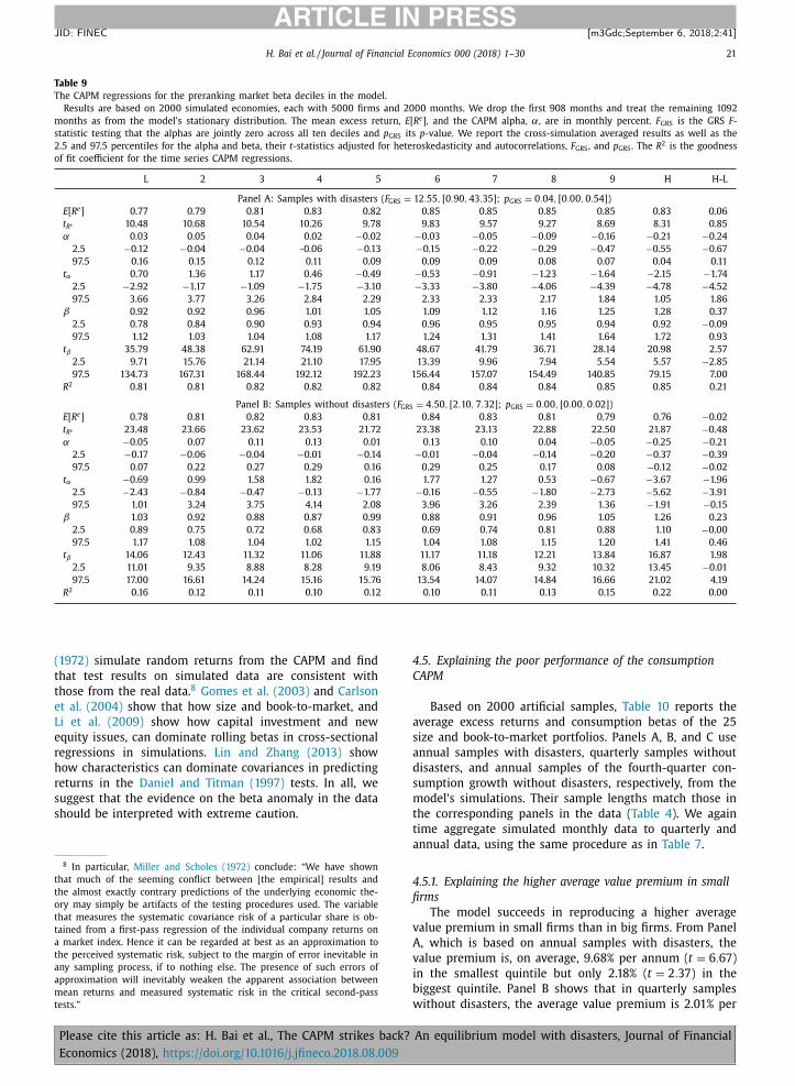
H. Bai et al. / Journal of Financial Economics 0 0 0 (2018) 1–30 21
ARTICLE IN PRESS
JID: FINEC [m3Gdc; September 6, 2018;2:41 ]
Table 9
The CAPM regressions for the preranking market beta deciles in the model.
Results are based on 20 0 0 simulated economies, each with 50 0 0 firms and 20 0 0 months. We drop the first 908 months and treat the remaining 1092
months as from the model’s stationary distribution. The mean excess return, E [ R e ], and the CAPM alpha, α, are in monthly percent. F GRS is the GRS F -
statistic testing that the alphas are jointly zero across all ten deciles and p GRS its p -value. We report the cross-simulation averaged results as well as the
2.5 and 97.5 percentiles for the alpha and beta, their t -statistics adjusted for heteroskedasticity and autocorrelations, F GRS , and p GRS . The R 2 is the goodness
of fit coefficient for the time series CAPM regressions.
L 2 3 4 5 6 7 8 9 H H-L
Panel A: Samples with disasters ( F GRS = 12 . 55 , [0 . 90 , 43 . 35] ; p GRS = 0 . 04 , [0 . 00 , 0 . 54] )
E [ R e ] 0.77 0.79 0.81 0.83 0.82 0.85 0.85 0.85 0.85 0.83 0.06
t R e 10.48 10.68 10.54 10.26 9.78 9.83 9.57 9.27 8.69 8.31 0.85
α 0.03 0.05 0.04 0.02 −0.02 −0.03 −0.05 −0.09 −0.16 −0.21 −0.24
2.5 −0.12 −0.04 −0.04 -0.06 −0.13 −0.15 −0.22 −0.29 −0.47 −0.55 −0.67
97.5 0.16 0.15 0.12 0.11 0.09 0.09 0.09 0.08 0.07 0.04 0.11
t α 0.70 1.36 1.17 0.46 −0.49 −0.53 −0.91 −1.23 −1.64 −2.15 −1.74
2.5 −2.92 −1.17 −1.09 −1.75 −3.10 −3.33 −3.80 −4.06 −4.39 −4.78 −4.52
97.5 3.66 3.77 3.26 2.84 2.29 2.33 2.33 2.17 1.84 1.05 1.86
β 0.92 0.92 0.96 1.01 1.05 1.09 1.12 1.16 1.25 1.28 0.37
2.5 0.78 0.84 0.90 0.93 0.94 0.96 0.95 0.95 0.94 0.92 −0.09
97.5 1.12 1.03 1.04 1.08 1.17 1.24 1.31 1.41 1.64 1.72 0.93
t β 35.79 48.38 62.91 74.19 61.90 48.67 41.79 36.71 28.14 20.98 2.57
2.5 9.71 15.76 21.14 21.10 17.95 13.39 9.96 7.94 5.54 5.57 −2.85
97.5 134.73 167.31 168.44 192.12 192.23 156.44 157.07 154.49 140.85 79.15 7.00
R 2 0.81 0.81 0.82 0.82 0.82 0.84 0.84 0.84 0.85 0.85 0.21
Panel B: Samples without disasters ( F GRS = 4 . 50 , [2 . 10 , 7 . 32] ; p GRS = 0 . 00 , [0 . 00 , 0 . 02] )
E [ R e ] 0.78 0.81 0.82 0.83 0.81 0.84 0.83 0.81 0.79 0.76 −0.02
t R e 23.48 23.66 23.62 23.53 21.72 23.38 23.13 22.88 22.50 21.87 −0.48
α −0.05 0.07 0.11 0.13 0.01 0.13 0.10 0.04 −0.05 −0.25 −0.21
2.5 −0.17 −0.06 −0.04 −0.01 −0.14 −0.01 −0.04 −0.14 −0.20 −0.37 −0.39
97.5 0.07 0.22 0.27 0.29 0.16 0.29 0.25 0.17 0.08 −0.12 −0.02
t α −0.69 0.99 1.58 1.82 0.16 1.77 1.27 0.53 −0.67 −3.67 −1.96
2.5 −2.43 −0.84 −0.47 −0.13 −1.77 −0.16 −0.55 −1.80 −2.73 −5.62 −3.91
97.5 1.01 3.24 3.75 4.14 2.08 3.96 3.26 2.39 1.36 −1.91 −0.15
β 1.03 0.92 0.88 0.87 0.99 0.88 0.91 0.96 1.05 1.26 0.23
2.5 0.89 0.75 0.72 0.68 0.83 0.69 0.74 0.81 0.88 1.10 −0.00
97.5 1.17 1.08 1.04 1.02 1.15 1.04 1.08 1.15 1.20 1.41 0.46
t β 14.06 12.43 11.32 11.06 11.88 11.17 11.18 12.21 13.84 16.87 1.98
2.5 11.01 9.35 8.88 8.28 9.19 8.06 8.43 9.32 10.32 13.45 −0.01
97.5 17.00 16.61 14.24 15.16 15.76 13.54 14.07 14.84 16.66 21.02 4.19
R 2 0.16 0.12 0.11 0.10 0.12 0.10 0.11 0.13 0.15 0.22 0.00
(1972) simulate random returns from the CAPM and find
that test results on simulated data are consistent with
those from the real data. 8 Gomes et al. (2003) and Carlson
et al. (2004) show that how size and book-to-market, and
Li et al. (2009) show how capital investment and new
equity issues, can dominate rolling betas in cross-sectional
regressions in simulations. Lin and Zhang (2013) show
how characteristics can dominate covariances in predicting
returns in the Daniel and Titman (1997) tests. In all, we
suggest that the evidence on the beta anomaly in the data
should be interpreted with extreme caution.
8 In particular, Miller and Scholes (1972) conclude: “We have shown
that much of the seeming conflict between [the empirical] results and
the almost exactly contrary predictions of the underlying economic the-
ory may simply be artifacts of the testing procedures used. The variable
that measures the systematic covariance risk of a particular share is ob-
tained from a first-pass regression of the individual company returns on
a market index. Hence it can be regarded at best as an approximation to
the perceived systematic risk, subject to the margin of error inevitable in
any sampling process, if to nothing else. The presence of such errors of
approximation will inevitably weaken the apparent association between
mean returns and measured systematic risk in the critical second-pass
tests.”
Please cite this article as: H. Bai et al., The CAPM strikes back?
Economics (2018), https://doi.org/10.1016/j.jfineco.2018.08.009
4.5. Explaining the poor performance of the consumption
CAPM
Based on 20 0 0 artificial samples, Table 10 reports the
average excess returns and consumption betas of the 25
size and book-to-market portfolios. Panels A, B, and C use
annual samples with disasters, quarterly samples without
disasters, and annual samples of the fourth-quarter con-
sumption growth without disasters, respectively, from the
model’s simulations. Their sample lengths match those in
the corresponding panels in the data ( Table 4 ). We again
time aggregate simulated monthly data to quarterly and
annual data, using the same procedure as in Table 7 .
4.5.1. Explaining the higher average value premium in small
firms
The model succeeds in reproducing a higher average
value premium in small firms than in big firms. From Panel
A, which is based on annual samples with disasters, the
value premium is, on average, 9.68% per annum ( t = 6 . 67 )
in the smallest quintile but only 2.18% ( t = 2 . 37 ) in the
biggest quintile. Panel B shows that in quarterly samples
without disasters, the average value premium is 2.01% per
An equilibrium model with disasters, Journal of Financial

22 H. Bai et al. / Journal of Financial Economics 0 0 0 (2018) 1–30
ARTICLE IN PRESS
JID: FINEC [m3Gdc; September 6, 2018;2:41 ]
Table 10
The average excess returns and consumption betas for the 25 size and book-to-market portfolios in the model.
Results are based on 20 0 0 simulations, each with 50 0 0 firms and 20 0 0 months. We drop the first 908 months
and treat the remaining 1092 months as from the model’s stationary distribution. For each portfolio, we report
its average excess return, E [ R e ], and its consumption beta, βC , as well as their t -values adjusted for heteroskedas-
ticity and autocorrelations, t R e and t βC , respectively. Returns in Panels A and C are in annual percent and those
in Panel B in quarterly percent.
L 2 3 4 H L 2 3 4 H
Panel A: Annual samples with disasters
E [ R e ] t R e
Small 13.69 14.54 15.95 17.90 23.37 12.34 11.38 10.77 10.43 10.26
2 12.33 13.29 14.21 15.45 18.90 12.00 11.71 11.43 11.25 10.78
3 12.05 12.17 12.42 12.95 14.62 10.00 12.01 11.91 11.33 10.33
4 10.57 10.40 10.42 10.85 13.84 12.01 11.89 11.47 10.59 10.41
Big 7.96 7.92 8.18 8.86 10.14 10.16 9.96 9.80 9.67 9.23
βC t βC
Small −0.64 −0.77 −0.93 −1.15 −1.28 −0.61 −0.68 −0.72 −0.74 −0.47
2 −0.49 −0.59 −0.72 −0.89 −1.34 −0.55 −0.62 −0.69 −0.81 −0.97
3 −0.43 −0.47 −0.53 −0.64 −0.74 −0.50 −0.56 −0.63 −0.72 −0.70
4 −0.32 −0.33 −0.36 −0.46 −0.69 −0.41 −0.46 −0.52 −0.64 −0.79
Big −0.07 −0.08 −0.10 −0.22 −0.23 −0.01 −0.04 −0.08 −0.28 −0.09
Panel B: Quarterly samples without disasters
E [ R e ] t R e
Small 3.16 3.31 3.56 3.92 5.17 45.90 34.22 31.77 32.39 29.73
2 2.89 3.08 3.24 3.45 4.09 29.73 31.09 31.73 32.26 28.72
3 2.84 2.85 2.88 2.96 3.33 16.28 29.04 30.16 28.11 19.54
4 2.53 2.48 2.47 2.53 3.19 23.35 23.40 21.99 18.86 18.87
Big 1.93 1.91 1.96 2.07 2.42 13.66 13.75 14.14 15.06 14.71
βC t βC
Small 0.11 0.12 0.12 0.13 0.27 1.45 1.13 0.96 0.95 1.39
2 0.12 0.12 0.13 0.13 0.18 1.10 1.04 1.10 1.09 1.14
3 0.16 0.13 0.14 0.16 0.25 0.83 1.19 1.30 1.36 1.30
4 0.16 0.18 0.22 0.24 0.24 1.33 1.54 1.71 1.56 1.37
Big 0.74 0.93 1.08 0.94 0.85 4.83 6.32 7.60 6.51 4.74
Panel C: Annual samples with fourth-quarter consumption growth without disasters
E [ R e ] t R e
Small 13.54 14.20 15.34 17.00 22.80 43.01 32.13 30.08 30.64 28.12
2 12.35 13.21 13.91 14.86 17.76 28.37 29.75 30.32 30.72 27.52
3 12.13 12.15 12.28 12.63 14.31 15.79 27.81 28.90 26.74 18.91
4 10.75 10.53 10.48 10.72 13.66 22.29 22.50 21.19 18.31 18.16
Big 8.13 8.04 8.25 8.75 10.28 13.21 13.29 13.76 14.64 14.31
βC t βC
Small 0.21 0.23 0.22 0.24 0.50 1.55 1.23 0.99 1.01 1.42
2 0.24 0.22 0.24 0.25 0.31 1.27 1.17 1.23 1.18 1.11
3 0.27 0.22 0.24 0.26 0.35 0.83 1.17 1.30 1.28 1.07
4 0.26 0.28 0.30 0.32 0.36 1.21 1.38 1.38 1.27 1.09
Big 0.82 0.97 1.08 0.95 0.84 3.22 4.03 4.62 4.02 2.82
quarter ( t = 11 . 29 ) in the smallest quintile but only 0.49%
( t = 2 . 29 ) in the biggest quintile. The results from the an-
nual samples without disasters are largely similar (Panel
C).
The key mechanism underlying this result is decreas-
ing returns to scale. The curvature parameter, ξ , in the
production function in Eq. (5) is less than one (0.65 in
the benchmark calibration). As a result, the detrended cap-
ital, K it , is a firm-specific state variable in addition to
the firm-specific productivity, z it . With constant returns to
scale, ξ = 1 , the investment-to-capital ratio, I it / K it , is in-
dependent of capital, meaning that K it is not a separate
state variable. When ξ < 1, I it / K it clearly depends on
K it ,
with small firms investing faster than big firms ( Fig. 4 ).
Fig. 5 shows further that big spikes in risk and risk pre-
Please cite this article as: H. Bai et al., The CAPM strikes back?
Economics (2018), https://doi.org/10.1016/j.jfineco.2018.08.009
miums in the disaster states accrue to firms with small
capital stock and low firm-specific productivity. This pat-
tern implies that the expected return spread between the
low- and high- z it firms is higher in small- K it firms than in
big- K it firms.
The disaster risk also plays a role in reproducing the
higher value premium in small firms. The presence of
the disaster state and the subsequent recovery state en-
larges the cross-sectional dispersion in the detrended cap-
ital, making firms more heterogeneous. As a result, we can
perform independent sorts on size and book-to-market to
form the 25 portfolios in simulated samples.
Without showing the details, we can report that such
independent sorts are infeasible in the Lin and Zhang
(2013) model, which is in turn a simplified version of the
An equilibrium model with disasters, Journal of Financial
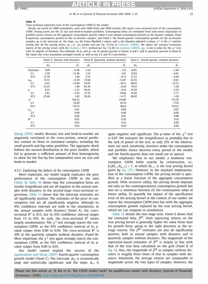
H. Bai et al. / Journal of Financial Economics 0 0 0 (2018) 1–30 23
ARTICLE IN PRESS
JID: FINEC [m3Gdc; September 6, 2018;2:41 ]
Table 11
Cross-sectional regression tests of the consumption CAPM in the model.
Results are based on 20 0 0 simulations, each with 50 0 0 firms and 20 0 0 months. We report cross-sectional tests of the consumption
CAPM. Testing assets are the 25 size and book-to-market portfolios. Consumption betas are estimated from time-series regressions of
portfolio excess returns on the aggregate consumption growth. Panel A uses annual consumption growth on the disaster samples, Panel
B quarterly consumption growth on the no-disaster samples, and Panel C the fourth-quarter consumption growth on the no-disaster
samples. φ0 is the intercept, φ1 the slope, t FM the Fama–MacBeth t -values, and t S the Shanken-adjusted t -values. χ2 is the χ2 -statistic
testing that all the pricing errors, φ0 + αi , are jointly zero per Eq. (12.14) in Cochrane (2005b) . We adjust the variance-covariance
matrix of the pricing errors with the Shanken (1992) method per Eq. (12.20) in Cochrane (2005b) . p χ2 is the p -value for the χ2 test,
with 23 degrees of freedom. The estimates of φ0 and φ1 are in annual percent in Panels A and C and in quarterly percent in Panel B.
We report the cross-simulation averaged results as well as the 2.5 and 97.5 percentiles.
Panel A: Annual, with disasters Panel B: Quarterly, without disasters Panel C: Fourth-quarter, without disasters
φ0 φ1 φ0 φ1 φ0 φ1
Estimates 9.09 −6 . 48 3.34 −1.19 14.05 −3.40
2.5 5.28 −13 . 46 3.14 −1.67 12.83 −6.81
97.5 13.70 1.46 3.53 −0.72 15.37 −0.48
t FM 15.57 −6 . 30 73.94 −13.67 63.93 −8.61
2.5 6.55 −12 . 84 53.97 −18.11 49.83 −15.53
97.5 52.25 1.48 83.30 −8.26 79.11 −1.28
t S 8.22 −3 . 31 44.22 −9.14 36.59 −5.33
2.5 3.81 −5 . 95 27.35 −10.94 19.28 −7.77
97.5 25.46 1.45 58.20 −6.77 60.92 −1.26
χ2 194.32 114.99 173.29
2.5 35.69 41.59 17.16
97.5 1171.4 418.4 1123.3
p χ2 0.01 0.00 0.07
2.5 0.00 0.00 0.00
97.5 0.04 0.01 0.80
R 2 0.61 0.30 0.16
2.5 0.01 0.12 0.00
97.5 0.95 0.49 0.46
Zhang (2005) model. Because size and book-to-market are
negatively correlated in the cross-section, several portfo-
lios contain no firms in simulated samples, including the
small-growth and big-value portfolios. The aggregate shock
follows the normal distribution in the prior models, which
fail to generate a sufficient amount of firm heterogeneity
to allow for the five-by-five independent sorts on size and
book-to-market.
4.5.2. Explaining the failure of the consumption CAPM
More important, our model largely replicates the poor
performance of the consumption CAPM in the data
( Table 4 ). Table 10 shows that the consumption betas are
mostly insignificant and are all negative in the annual sam-
ples with disasters. In the second-stage cross-sectional re-
gressions, Table 11 shows that the intercept estimates are
all significantly positive. The estimates of the price of con-
sumption risk are all significantly negative, although its
95% confidence intervals are wide in the simulations. In
the annual samples with disasters (Panel A), the cross-
sectional R 2 is 61%, but its 95% confidence interval ranges
from 1% to 95%. As such, the cross-sectional R 2 seems
largely uninformative. The χ2 test strongly rejects the con-
sumption CAPM, as the 95% confidence interval of its p -
value ranges from 0.00 to 0.04. The cross-sectional R 2 is
30% in the quarterly samples without disasters (Panel B).
More important, the χ2 test again strongly rejects the con-
sumption CAPM, as the 95% confidence interval of its p -
value ranges from 0.00 to 0.01.
Our model cannot explain the success of the
Jagannathan and Wang (2007) fourth-quarter consumption
growth model (Panel C). The intercept, φ0 , is economically
large and statistically significant, and the slope, φ , is
1Please cite this article as: H. Bai et al., The CAPM strikes back?
Economics (2018), https://doi.org/10.1016/j.jfineco.2018.08.009
again negative and significant. The p -value of the χ2 test
is 0.07. We interpret the insignificance as probably due to
the lack of power of the test, as only 25% of the observa-
tions are used. Intuitively, investors make the consumption
and portfolio choice decision every period in the model,
and the fourth-quarter does not stand out as special.
We emphasize that in our model, a nonlinear con-
sumption CAPM holds exactly by construction, i.e.,
E t [ M t+1 R it+1 ] = 1 , in which M t+1 is the true pricing kernel
given by Eq. (27) . However, in the standard implementa-
tion of the consumption CAPM, the pricing kernel is spec-
ified as a linear function of the aggregate consumption
growth. With recursive utility, the pricing kernel depends
not only on the contemporaneous consumption growth but
also on (a nonlinear function of) the continuation value of
future utility. To quantify the impact of the specification
error of the pricing kernel in the context of our model, we
repeat the consumption CAPM tests but with the aggregate
consumption growth replaced by the true pricing kernel,
which we can compute in simulations.
Table 12 details the two-stage tests. Panel A shows that
the estimated beta, ˆ βM , from regressing returns on the
true pricing kernel is generally higher for value firms than
for growth firms, going in the right direction as the av-
erage returns. The ˆ βM estimates are also all significantly
positive, both in annual samples with disasters and in
quarterly samples without disasters. The magnitude of the
regression-based estimates of ˆ βM is largely in line with
that of the true beta calculated on the grid (Panel D of
Fig. 6 ). Also, the magnitude of ˆ βM in samples without dis-
asters is roughly three times of that in samples with dis-
asters. Intuitively, the average returns are comparable in
magnitude across the two types of samples. However, the
An equilibrium model with disasters, Journal of Financial
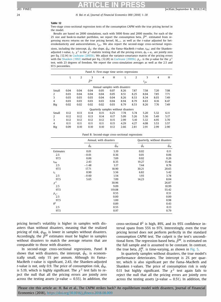
24 H. Bai et al. / Journal of Financial Economics 0 0 0 (2018) 1–30
ARTICLE IN PRESS
JID: FINEC [m3Gdc; September 6, 2018;2:41 ]
Table 12
Two-stage cross-sectional regression tests of the consumption CAPM with the true pricing kernel in
the model.
Results are based on 20 0 0 simulations, each with 50 0 0 firms and 20 0 0 months. For each of the
25 size and book-to-market portfolios, we report the consumption beta, ˆ βM , estimated from re-
gressing excess returns on the true pricing kernel, M t+1 , as well as the t -value adjusted for het-
eroskedasticity and autocorrelations, t ˆ βM . We also report the second-stage cross-sectional regres-
sions, including the intercept, ˆ φ0 ; the slope, ˆ φM ; the Fama–MacBeth t -value, t FM ; and the Shanken-
adjusted t -value, t S . χ2 is the χ2 -statistic testing that all the pricing errors, φ0 + αi , are jointly zero
per Eq. (12.14) in Cochrane (2005b) . We adjust the variance-covariance matrix of the pricing errors
with the Shanken (1992) method per Eq. (12.20) in Cochrane (2005b) . p χ2 is the p -value for the χ2
test, with 23 degrees of freedom. We report the cross-simulation averages as well as the 2.5 and
97.5 percentiles.
Panel A: First-stage time series regressions
L 2 3 4 H L 2 3 4 H
ˆ βM t ˆ βM
Annual samples with disasters
Small 0.04 0.04 0.04 0.05 0.07 8.26 7.87 7.58 7.20 7.08
2 0.03 0.04 0.04 0.04 0.05 8.51 8.25 8.04 7.85 7.71
3 0.03 0.03 0.03 0.04 0.04 8.26 8.53 8.34 8.03 7.49
4 0.03 0.03 0.03 0.03 0.04 8.94 8.79 8.63 8.16 8.47
Big 0.02 0.02 0.02 0.02 0.03 8.79 8.53 8.26 7.76 7.49
Quarterly samples without disasters
Small 0.12 0.13 0.14 0.15 0.25 7.78 5.74 5.20 5.32 6.11
2 0.12 0.12 0.13 0.14 0.17 5.09 5.26 5.36 5.49 5.17
3 0.12 0.12 0.12 0.12 0.15 2.99 5.10 5.32 4.95 3.70
4 0.11 0.11 0.11 0.11 0.15 4.29 4.27 4.08 3.53 3.57
Big 0.09 0.10 0.10 0.10 0.12 2.66 2.81 2.91 2.99 2.90
Panel B: Second-stage cross-sectional regressions
Annual, with disasters Quarterly, without disasters
ˆ φ0 ˆ φM
ˆ φ0 ˆ φM
Estimates 0.01 5.19 0.02 0.11
2.5 −0 . 01 0.36 0.01 0.06
97.5 0.06 7.69 0.02 0.26
t FM 2.43 8.35 19.27 15.46
2.5 −1 . 48 3.17 7.44 8.76
97.5 17.71 18.90 30.21 20.65
t S 0.90 3.56 6.82 5.42
2.5 −0 . 60 1.54 1.93 3.78
97.5 5.65 7.09 14.23 8.04
χ2 30.96 26.87
2.5 9.09 10.99
97.5 119.08 55.42
p χ2 0.55 0.51
2.5 0.00 0.00
97.5 1.00 0.98
R 2 0.89 0.43
2.5 0.55 0.13
97.5 0.97 0.79
pricing kernel’s volatility is higher in samples with dis-
asters than without disasters, meaning that the realized
pricing of risk, φMt , is lower in samples without disasters.
Accordingly, the ˆ βM estimates must be higher in samples
without disasters to match the average returns that are
comparable to those with disasters.
In second-stage cross-sectional regressions, Panel B
shows that with disasters, the intercept, ˆ φ0 , is econom-
ically small, only 1% per annum. Although its Fama–
MacBeth t -value is significant, 2.43, the Shanken-adjusted
t -value is not, only 0.9. The price of consumption risk, ˆ φM
,
is 5.19, which is highly significant. The χ2 test fails to re-
ject the null that all the pricing errors are jointly zero
across the testing assets ( p -value = 0.55). In addition, the
Please cite this article as: H. Bai et al., The CAPM strikes back?
Economics (2018), https://doi.org/10.1016/j.jfineco.2018.08.009
cross-sectional R 2 is high, 89%, and its 95% confidence in-
terval spans from 55% to 97%. Interestingly, even the true
pricing kernel does not perform perfectly in the standard
consumption CAPM test. The culprit is the test’s uncondi-
tional form. The regression-based beta, ˆ βM , is estimated on
the full sample and is assumed to be constant. In contrast,
the true beta, βM
it , is time-varying, as shown in Fig. 5 .
In quarterly samples without disasters, the true model’s
performance deteriorates. The intercept is 2% per quar-
ter, which is also significant per the Fama–MacBeth and
Shanken t -values. The price of consumption risk is only
0.11 but highly significant. The χ2 test again fails to
reject the null that all the pricing errors are jointly zero
across the testing assets ( p -value = 0.51). In addition, the
An equilibrium model with disasters, Journal of Financial
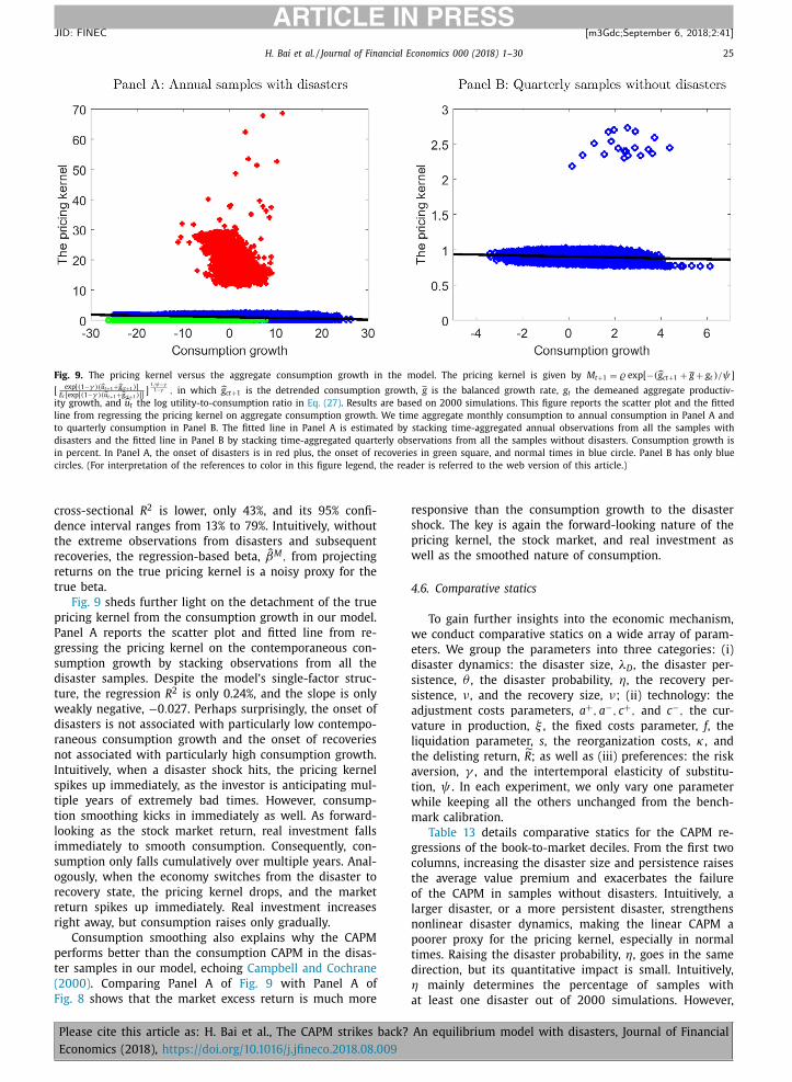
H. Bai et al. / Journal of Financial Economics 0 0 0 (2018) 1–30 25
ARTICLE IN PRESS
JID: FINEC [m3Gdc; September 6, 2018;2:41 ]
Fig. 9. The pricing kernel versus the aggregate consumption growth in the model. The pricing kernel is given by M t+1 = � exp [ −( g ct+1 + g + g t ) /ψ]
[ exp [(1 −γ )( u t+1 + g ct+1 )] E t [ exp [(1 −γ )( u t+1 + g ct+1 )]]
] 1 /ψ−γ
1 −γ , in which g ct+1 is the detrended consumption growth, g is the balanced growth rate, g t the demeaned aggregate productiv-
ity growth, and u t the log utility-to-consumption ratio in Eq. (27) . Results are based on 20 0 0 simulations. This figure reports the scatter plot and the fitted
line from regressing the pricing kernel on aggregate consumption growth. We time aggregate monthly consumption to annual consumption in Panel A and
to quarterly consumption in Panel B. The fitted line in Panel A is estimated by stacking time-aggregated annual observations from all the samples with
disasters and the fitted line in Panel B by stacking time-aggregated quarterly observations from all the samples without disasters. Consumption growth is
in percent. In Panel A, the onset of disasters is in red plus, the onset of recoveries in green square, and normal times in blue circle. Panel B has only blue
circles. (For interpretation of the references to color in this figure legend, the reader is referred to the web version of this article.)
cross-sectional R 2 is lower, only 43%, and its 95% confi-
dence interval ranges from 13% to 79%. Intuitively, without
the extreme observations from disasters and subsequent
recoveries, the regression-based beta, ˆ βM , from projecting
returns on the true pricing kernel is a noisy proxy for the
true beta.
Fig. 9 sheds further light on the detachment of the true
pricing kernel from the consumption growth in our model.
Panel A reports the scatter plot and fitted line from re-
gressing the pricing kernel on the contemporaneous con-
sumption growth by stacking observations from all the
disaster samples. Despite the model’s single-factor struc-
ture, the regression R 2 is only 0.24%, and the slope is only
weakly negative, −0 . 027 . Perhaps surprisingly, the onset of
disasters is not associated with particularly low contempo-
raneous consumption growth and the onset of recoveries
not associated with particularly high consumption growth.
Intuitively, when a disaster shock hits, the pricing kernel
spikes up immediately, as the investor is anticipating mul-
tiple years of extremely bad times. However, consump-
tion smoothing kicks in immediately as well. As forward-
looking as the stock market return, real investment falls
immediately to smooth consumption. Consequently, con-
sumption only falls cumulatively over multiple years. Anal-
ogously, when the economy switches from the disaster to
recovery state, the pricing kernel drops, and the market
return spikes up immediately. Real investment increases
right away, but consumption raises only gradually.
Consumption smoothing also explains why the CAPM
performs better than the consumption CAPM in the disas-
ter samples in our model, echoing Campbell and Cochrane
(20 0 0) . Comparing Panel A of Fig. 9 with Panel A of
Fig. 8 shows that the market excess return is much more
Please cite this article as: H. Bai et al., The CAPM strikes back?
Economics (2018), https://doi.org/10.1016/j.jfineco.2018.08.009
responsive than the consumption growth to the disaster
shock. The key is again the forward-looking nature of the
pricing kernel, the stock market, and real investment as
well as the smoothed nature of consumption.
4.6. Comparative statics
To gain further insights into the economic mechanism,
we conduct comparative statics on a wide array of param-
eters. We group the parameters into three categories: (i)
disaster dynamics: the disaster size, λD , the disaster per-
sistence, θ , the disaster probability, η, the recovery per-
sistence, ν , and the recovery size, ν; (ii) technology: the
adjustment costs parameters, a + , a −, c + , and c −, the cur-
vature in production, ξ , the fixed costs parameter, f , the
liquidation parameter, s , the reorganization costs, κ , and
the delisting return, ˜ R ; as well as (iii) preferences: the risk
aversion, γ , and the intertemporal elasticity of substitu-
tion, ψ . In each experiment, we only vary one parameter
while keeping all the others unchanged from the bench-
mark calibration.
Table 13 details comparative statics for the CAPM re-
gressions of the book-to-market deciles. From the first two
columns, increasing the disaster size and persistence raises
the average value premium and exacerbates the failure
of the CAPM in samples without disasters. Intuitively, a
larger disaster, or a more persistent disaster, strengthens
nonlinear disaster dynamics, making the linear CAPM a
poorer proxy for the pricing kernel, especially in normal
times. Raising the disaster probability, η, goes in the same
direction, but its quantitative impact is small. Intuitively,
η mainly determines the percentage of samples with
at least one disaster out of 20 0 0 simulations. However,
An equilibrium model with disasters, Journal of Financial
26 H. Bai et al. / Journal of Financial Economics 0 0 0 (2018) 1–30
ARTICLE IN PRESS
JID: FINEC [m3Gdc; September 6, 2018;2:41 ]
Table 13
Comparative statics, the CAPM regressions of the book-to-market deciles.
Results are averaged across 20 0 0 simulations. E [ R e ] is the average return, α the CAPM alpha, and β the market beta of the value-minus-growth decile.
E [ R e ] and α are in monthly percent. The t -values are adjusted for heteroskedasticity and autocorrelations. Each column shows results from one experiment.
In each column, we vary only one parameter while keeping the others unchanged from the benchmark calibration. The alternative parameter values in the
comparative statics are λD = −3 . 25% , θ = 0 . 985 , η = 3% / 12 , ν = 0 . 98 , λR = 2% , a + = 0 . 045 , a − = 0 . 065 , c + = 100 , c − = 200 , ξ = 0 . 7 , f = 0 . 01 , s = 0 . 15 ,
κ = 0 . 35 , R = −16% , γ = 6 , and ψ = 2 . The simulation design in each experiment is identical to that in Table 8 .
λD θ η ν λR a + a − c + c − ξ f s κ ˜ R γ ψ
Panel A: Samples with disasters
E [ R e ] 0.75 0.41 0.49 0.45 0.45 0.30 0.53 0.44 0.43 0.38 0.51 0.22 0.39 0.44 0.55 0.52
t R e 6.67 4.29 4.87 4.54 4.75 3.68 5.17 4.72 4.53 5.09 5.09 3.60 4.31 4.72 6.35 4.55
α −0.46 −0.63 −0.32 −0.37 −0.35 −0.25 −0 . 34 −0 . 34 −0.39 −0.52 −0.29 −0.19 −0 . 39 −0.36 −0 . 40 −0.44
t α −2.47 −2.96 −2.34 −2.62 −2.49 −2.10 −2 . 37 −2 . 58 −2.65 −2.88 −2.11 −2.08 −2 . 69 −2.49 −2 . 41 −2.65
β 1.09 1.08 1.03 1.00 0.99 0.69 1.08 1.05 1.04 1.11 1.00 0.54 0.98 1.01 0.95 0.98
t β 8.04 8.40 8.08 8.07 7.91 6.85 7.87 7.97 8.11 7.66 7.85 7.86 8.10 8.01 7.66 7.89
Panel B: Samples without disasters
E [ R e ] 0.62 0.53 0.42 0.39 0.39 0.21 0.41 0.37 0.40 0.40 0.41 0.22 0.37 0.39 0.52 0.43
t R e 10.84 9.53 7.95 7.52 7.55 3.94 7.95 7.63 7.69 10.40 7.46 4.45 7.14 7.51 9.36 8.07
α 0.51 0.44 0.31 0.26 0.25 −0.06 0.28 0.31 0.26 0.22 0.23 0.15 0.22 0.25 0.40 0.34
t α 3.26 3.07 2.71 2.28 2.22 −0.61 2.47 2.98 2.34 2.08 1.93 1.37 1.98 2.22 2.79 2.75
β 0.09 0.09 0.14 0.17 0.17 0.34 0.16 0.08 0.17 0.21 0.23 0.09 0.18 0.18 0.11 0.10
t β 0.68 0.65 1.12 1.35 1.41 2.94 1.23 0.59 1.37 1.74 1.79 0.76 1.48 1.40 0.86 0.85
Table 14
Comparative statics, the CAPM regressions of the preranking market beta deciles.
Results are averaged across 20 0 0 simulations. E [ R e ] is the average return, α the CAPM alpha, and β the market beta of the high-minus-low market beta
decile. E [ R e ] and α are in monthly percent. The t -values are adjusted for heteroskedasticity and autocorrelations. Each column shows results from one
experiment. In each column, we vary only one parameter while keeping the others unchanged from the benchmark calibration. The alternative parameter
values in the comparative statics are λD = −3 . 25% , θ = 0 . 985 , η = 3% / 12 , ν = 0 . 98 , λR = 2% , a + = 0 . 045 , a − = 0 . 065 , c + = 100 , c − = 200 , ξ = 0 . 7 , f = 0 . 01 ,
s = 0 . 15 , κ = 0 . 35 , R = −16% , γ = 6 , and ψ = 2 . The simulation design in each experiment is identical to that in Table 9 .
λD θ η ν λR a + a − c + c − ξ f s κ ˜ R γ ψ
Panel A: Samples with disasters
E [ R e ] 0.08 0.01 0.08 0.07 0.07 0.05 0.07 0.06 0.06 0.03 0.06 −0 . 81 0.06 0.06 0.06 0.06
t R e 1.00 0.25 1.08 0.97 0.92 0.68 0.90 0.88 0.83 0.88 0.86 −4 . 26 0.84 0.84 0.84 0.84
α −0 . 30 −0 . 22 −0 . 20 −0 . 24 −0 . 24 −0 . 22 −0 . 24 −0 . 23 −0 . 24 −0 . 25 −0 . 24 −1 . 09 −0 . 24 −0 . 24 −0 . 24 −0 . 24
t α −1 . 69 −1 . 47 −1 . 62 −1 . 81 −1 . 74 −1 . 68 −1 . 70 −1 . 71 −1 . 78 −1 . 86 −1 . 73 −3 . 23 −1 . 74 −1 . 76 −1 . 77 −1 . 74
β 0.33 0.24 0.35 0.38 0.37 0.33 0.37 0.37 0.37 0.34 0.37 0.66 0.37 0.37 0.37 0.37
t β 2.46 2.28 2.56 2.79 2.62 2.29 2.56 2.53 2.63 2.92 2.58 3.18 2.56 2.61 2.55 2.59
Panel B: Samples without disasters
E [ R e ] −0 . 03 −0 . 03 −0 . 02 −0 . 02 −0 . 01 −0 . 03 −0 . 02 −0 . 02 −0 . 02 0.00 −0 . 02 −0 . 07 −0 . 02 −0 . 02 −0 . 02 −0 . 02
t R e −0 . 50 −0 . 55 −0 . 48 −0 . 51 −0 . 29 −0 . 52 −0 . 34 −0 . 32 −0 . 47 0.01 −0 . 48 −1 . 38 −0 . 47 −0 . 49 −0 . 40 −0 . 49
α −0 . 27 −0 . 25 −0 . 21 −0 . 21 −0 . 20 −0 . 21 −0 . 19 −0 . 19 −0 . 21 −0 . 16 −0 . 21 −0 . 25 −0 . 21 −0 . 21 −0 . 20 −0 . 21
t α −1 . 89 −1 . 90 −2 . 00 −1 . 97 −1 . 85 −2 . 04 −1 . 82 −1 . 80 −1 . 98 −1 . 53 −1 . 95 −2 . 42 −1 . 95 −1 . 97 −1 . 90 −1 . 97
β 0.22 0.22 0.23 0.23 0.23 0.23 0.22 0.22 0.23 0.19 0.23 0.24 0.23 0.23 0.23 0.23
t β 1.87 1.87 2.03 1.98 1.97 2.13 1.89 1.89 2.01 1.72 1.98 2.09 1.97 1.99 2.02 1.99
conditioning on at least one disaster appearing in a given
sample, the nonlinear dynamics are mostly governed by
the disaster size and persistence.
The recovery size and persistence have little impact on
the magnitude of the average value premium and the per-
formance of the CAPM. Intuitively, risk and risk premiums
are mostly determined by the dynamics in bad times, par-
ticularly disasters, in which the representative household’s
marginal utility is the highest. In contrast, the marginal
utility is the lowest in the recovery state, giving rise to
small spreads in risk and risk premium between value and
growth firms.
The upward nonconvex costs parameter, a + , and its
downward counterpart, a −, work in the opposite direc-
tion. While increasing a + reduces the average value pre-
mium and its CAPM alpha in normal times, increasing a −
does the opposite. Intuitively, the a − effect works through
Please cite this article as: H. Bai et al., The CAPM strikes back?
Economics (2018), https://doi.org/10.1016/j.jfineco.2018.08.009
the asymmetry mechanism. A high value of a − means that
value firms face a higher hurdle in reducing their unpro-
ductive capital in the disaster state, giving rise to higher
risk and risk premiums.
Why does the upward nonconvex costs parameter, a + , work differently? Intuitively, firms disinvest very infre-
quently. Across simulations, on average, only 0.6% of the
firm-month observations have negative investment. Such a
low disinvestment frequency means that a + is the main
parameter that determines the magnitude of nonconvex
adjustment costs, a + K it . A lower a + means that firms
would in general have higher capital, especially value
firms. When a disaster hits, value firms are burdened
with more unproductive capital, reinforcing the asymmetry
mechanism. As such, a lower a + value increases the aver-
age value premium and its CAPM alpha in the no-disaster
samples.
An equilibrium model with disasters, Journal of Financial
H. Bai et al. / Journal of Financial Economics 0 0 0 (2018) 1–30 27
ARTICLE IN PRESS
JID: FINEC [m3Gdc; September 6, 2018;2:41 ]
Table 15
Comparative statics, the consumption CAPM test on the 25 size and book-to-market portfolios.
Results are averaged across 20 0 0 simulations. We report cross-sectional tests of the consumption CAPM. Testing assets are the 25 size and book-to-market
portfolios. Consumption betas are from time series regressions of portfolio excess returns on the aggregate consumption growth. Panel A uses annual
consumption growth on the disaster samples and Panel B quarterly consumption growth on the no-disaster samples. φ0 is the intercept, φ1 the slope, t FM
the Fama–MacBeth t -values, and t S the Shanken-adjusted t -values. χ2 is the χ2 -statistic testing that all the pricing errors, φ0 + αi , are jointly zero per Eq.
(12.14) in Cochrane (2005b) . We adjust the variance-covariance matrix of the pricing errors with the Shanken (1992) method per Eq. (12.20) in Cochrane
(2005b) . p χ2 is the p -value for the χ2 test, with 23 degrees of freedom. The estimates of φ0 and φ1 are in annual percent in Panel A and in quarterly
percent in Panel B. Each column shows results from one experiment. In each column, we vary only one parameter while keeping the others unchanged from
the benchmark calibration. The alternative parameter values are λD = −3 . 25% , θ = 0 . 985 , η = 3% / 12 , ν = 0 . 98 , λR = 2% , a + = 0 . 045 , a − = 0 . 065 , c + = 100 ,
c − = 200 , ξ = 0 . 7 , f = 0 . 01 , s = 0 . 15 , κ = 0 . 35 , R = −16% , γ = 6 , and ψ = 2 .
λD θ η ν λR a + a − c + c − ξ f s κ ˜ R γ ψ
Panel A: Annual samples with disasters
φ0 9.04 10.06 8.62 9.16 9.66 9.01 9.02 8.91 9.04 8.95 8.96 10.26 9,01 9.01 8.91 9.02
t FM 14.53 12.59 12.72 13.97 14.35 15.22 15.22 14.99 15.53 15.32 15.31 13.35 15.18 15.18 15.06 15.27
t S 7.92 7.63 6.95 7.35 7.52 7.97 7.97 7.90 8.09 7.98 8.02 9.96 7.98 7.97 7.86 7.94
φ1 −7 . 15 −5 . 64 −7 . 06 −7 . 68 −7 . 91 −6 . 57 −6 . 56 −6 . 62 −6 . 57 −6 . 23 −6 . 59 −3 . 17 −6 . 55 −6 . 55 −6 . 57 −6 . 65
t FM −6 . 56 −4 . 64 −5 . 80 −5 . 99 −6 . 29 −6 . 37 −6 . 37 −6 . 38 −6 . 42 −6 . 37 −6 . 40 −4 . 74 −6 . 35 −6 . 31 −6 . 33 −6 . 42
t S −3 . 71 −2 . 65 −3 . 17 −3 . 09 −3 . 26 −3 . 32 −3 . 32 −3 . 33 −3 . 37 −3 . 32 −3 . 35 −3 . 90 −3 . 32 −3 . 29 −3 . 30 −3 . 34
χ2 166.8 208.8 132.1 147.5 157.8 174.2 174.5 172.8 183.2 186.9 181.0 464.7 175.07 174.5 170.81 174.9
p χ2 0.01 0.01 0.01 0.01 0.01 0.01 0.01 0.01 0.01 0.01 0.01 0.00 0.01 0.01 0.01 0.01
R 2 0.66 0.48 0.66 0.64 0.64 0.63 0.62 0.63 0.62 0.63 0.63 0.56 0.62 0.62 0.63 0.63
Panel B: Quarterly samples without disasters
φ0 3.34 3.34 3.34 3.33 3.34 3.34 3.34 3.34 3.34 3.35 3.34 2.99 3.34 3.34 3.34 3.34
t FM 73.61 73.86 72.80 73.25 73.42 73.48 73.57 73.82 74.28 73.25 73.27 60.72 73.57 73.47 74.04 73.42
t S 44.17 43.88 43.33 43.42 43.96 44.05 44.10 44.43 44.12 44.02 44.05 38.75 44.20 43.98 44.23 43.87
φ1 −1 . 19 −1 . 21 −1 . 20 −1 . 28 −1 . 21 −1 . 19 −1 . 19 −1 . 18 −1 . 21 −0 . 99 −1 . 19 −1 . 09 −1 . 19 −1 . 19 −1 . 20 −1 . 19
t FM −13 . 64 −13 . 79 −13 . 75 −13 . 78 −13 . 66 −13 . 65 −13 . 66 −13 . 59 −13 . 81 −13 . 15 −13 . 58 −11 . 06 −13 . 61 −13 . 68 −13 . 73 −13 . 66
t S −9 . 16 −9 . 14 −9 . 16 −9 . 06 −9 . 13 −9 . 16 −9 . 17 −9 . 15 −9 . 19 −8 . 74 −9 . 12 −7 . 64 −9 . 14 −9 . 17 −9 . 17 −9 . 15
χ2 123.0 135.6 96.7 107.3 136.5 112.9 112.5 114.1 116.2 110.0 111.2 242.4 112.40 112.7 117.60 112.1
p χ2 0.00 0.00 0.00 0.00 0.00 0.00 0.00 0.00 0.00 0.00 0.00 0.00 0.00 0.00 0.00 0.00
R 2 0.29 0.30 0.30 0.30 0.29 0.29 0.29 0.29 0.30 0.27 0.29 0.40 0.29 0.30 0.30 0.29
Table 11 .
Similarly, the upward and downward convex costs pa-
rameters, c + and c −, respectively, work in the opposite
direction, but their impact is small. A higher c − works
through the asymmetry mechanism by restricting the flex-
ibility of value firms in downsizing in disasters, giving rise
to higher risk and risk premiums. However, because of the
vast majority of positive investment, the upward parame-
ter, c + , mainly determines the magnitude of convex costs.
A lower c + implies that firms have more capital in general,
especially value firms, reinforcing the asymmetry mecha-
nism.
In addition, increasing the curvature parameter, ξ , in-
creases the value premium in the no-disaster samples. In-
creasing the fixed costs parameter, f , raises the value pre-
mium but decreases its CAPM alpha in the no-disaster
samples. A higher f means a higher operating leverage for
value firms, increasing the value premium ( Carlson et al.,
2004 ). However, a higher f also means higher market beta
for the value premium, decreasing its CAPM alpha.
The next three technological parameters involve entry
and exit, including the liquidation value, s , the reorgani-
zation costs, κ , and the delisting return, ˜ R . Increasing s
reduces the average value premium and its CAPM alpha.
Intuitively, with a higher s , in the event of exit, share-
holders get to extract a higher liquidation value of sK it ,
which is in effect a free abandonment option. This option
acts as an insurance against the disaster risk. The aban-
donment option is especially attractive for shareholders of
value firms, which tend to have more unproductive capital
than growth firms. Consequently, instead of facing asym-
metric adjustment costs in disasters, the shareholders opt
Please cite this article as: H. Bai et al., The CAPM strikes back?
Economics (2018), https://doi.org/10.1016/j.jfineco.2018.08.009
to exit, thereby reducing the risk for value firms relative to
growth firms.
In addition, a higher reorganization cost, κ , reduces the
value premium and its CAPM alpha, but the effect is small
in the no-disaster samples. The impact of the delisting
return, ˜ R , is negligible. Finally, increasing the risk aver-
sion, γ , or the intertemporal elasticity of substitution, ψ ,
strengthens the nonlinear dynamics, raising the value pre-
mium and its CAPM alpha in the no-disaster samples.
For completeness, Table 14 reports comparative statics
for the market beta deciles. The results are quantitatively
similar to those in the benchmark calibration. The only ex-
ception is the liquidation value parameter, s . Raising s from
zero to 15% reduces the average return of the high-minus-
low market beta decile from 0.06% per month ( t = 0 . 85 )
in the benchmark calibration to −0 . 81% ( t = −4 . 26 ) in the
disaster samples in Panel A. As noted, a positive s gives the
shareholders an abandonment option, which reduces risk
and risk premiums. The low beta decile earns 0.59% (unt-
abulated), which is lower than 0.77% with s = 0 . More im-
portant, the high beta decile earns only −0 . 22% , which is
substantially lower than 0.83% with s = 0 . Intuitively, with
a higher s at 15%, many high beta stocks exit the econ-
omy in the disaster state, taking the large negative delist-
ing return of −12 . 33% . This effect is largely absent in Panel
B without disasters.
Finally, Table 15 reports comparative statics for the con-
sumption CAPM tests. Without going through the details,
we can report that the quantitative results are largely
similar to those in the benchmark calibration shown in
An equilibrium model with disasters, Journal of Financial
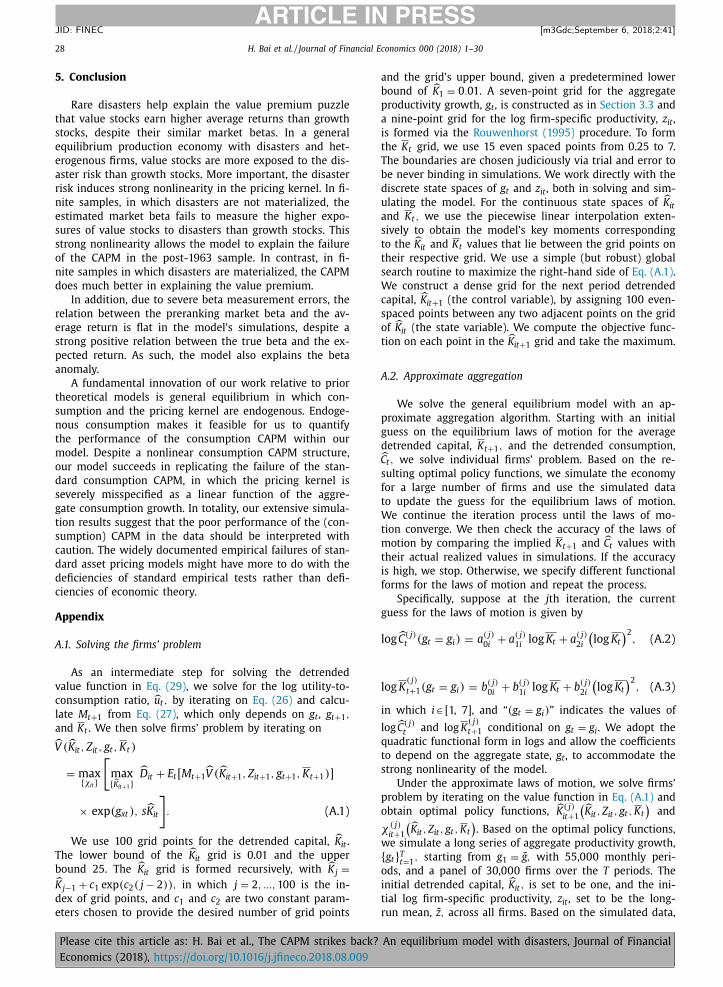
28 H. Bai et al. / Journal of Financial Economics 0 0 0 (2018) 1–30
ARTICLE IN PRESS
JID: FINEC [m3Gdc; September 6, 2018;2:41 ]
V
5. Conclusion
Rare disasters help explain the value premium puzzle
that value stocks earn higher average returns than growth
stocks, despite their similar market betas. In a general
equilibrium production economy with disasters and het-
erogenous firms, value stocks are more exposed to the dis-
aster risk than growth stocks. More important, the disaster
risk induces strong nonlinearity in the pricing kernel. In fi-
nite samples, in which disasters are not materialized, the
estimated market beta fails to measure the higher expo-
sures of value stocks to disasters than growth stocks. This
strong nonlinearity allows the model to explain the failure
of the CAPM in the post-1963 sample. In contrast, in fi-
nite samples in which disasters are materialized, the CAPM
does much better in explaining the value premium.
In addition, due to severe beta measurement errors, the
relation between the preranking market beta and the av-
erage return is flat in the model’s simulations, despite a
strong positive relation between the true beta and the ex-
pected return. As such, the model also explains the beta
anomaly.
A fundamental innovation of our work relative to prior
theoretical models is general equilibrium in which con-
sumption and the pricing kernel are endogenous. Endoge-
nous consumption makes it feasible for us to quantify
the performance of the consumption CAPM within our
model. Despite a nonlinear consumption CAPM structure,
our model succeeds in replicating the failure of the stan-
dard consumption CAPM, in which the pricing kernel is
severely misspecified as a linear function of the aggre-
gate consumption growth. In totality, our extensive simula-
tion results suggest that the poor performance of the (con-
sumption) CAPM in the data should be interpreted with
caution. The widely documented empirical failures of stan-
dard asset pricing models might have more to do with the
deficiencies of standard empirical tests rather than defi-
ciencies of economic theory.
Appendix
A.1. Solving the firms’ problem
As an intermediate step for solving the detrended
value function in Eq. (29) , we solve for the log utility-to-
consumption ratio, u t , by iterating on Eq. (26) and calcu-
late M t+1 from Eq. (27) , which only depends on g t , g t+1 ,
and K t . We then solve firms’ problem by iterating on ( K it , Z it , g t , K t )
= max { χit }
[max { K it+1 }
D it + E t [ M t+1 V ( K it+1 , Z it+1 , g t+1 , K t+1 )]
× exp (g xt ) , s K it
]. (A.1)
We use 100 grid points for the detrended capital, K it .
The lower bound of the K it grid is 0.01 and the upper
bound 25. The K it grid is formed recursively, with
K j = K j−1 + c 1 exp (c 2 ( j − 2)) , in which j = 2 , ..., 100 is the in-
dex of grid points, and c 1 and c 2 are two constant param-
eters chosen to provide the desired number of grid points
Please cite this article as: H. Bai et al., The CAPM strikes back?
Economics (2018), https://doi.org/10.1016/j.jfineco.2018.08.009
and the grid’s upper bound, given a predetermined lower
bound of K 1 = 0 . 01 . A seven-point grid for the aggregate
productivity growth, g t , is constructed as in Section 3.3 and
a nine-point grid for the log firm-specific productivity, z it ,
is formed via the Rouwenhorst (1995) procedure. To form
the K t grid, we use 15 even spaced points from 0.25 to 7.
The boundaries are chosen judiciously via trial and error to
be never binding in simulations. We work directly with the
discrete state spaces of g t and z it , both in solving and sim-
ulating the model. For the continuous state spaces of K it
and K t , we use the piecewise linear interpolation exten-
sively to obtain the model’s key moments corresponding
to the K it and K t values that lie between the grid points on
their respective grid. We use a simple (but robust) global
search routine to maximize the right-hand side of Eq. (A.1) .
We construct a dense grid for the next period detrended
capital, K it+1 (the control variable), by assigning 100 even-
spaced points between any two adjacent points on the grid
of K it (the state variable). We compute the objective func-
tion on each point in the K it+1 grid and take the maximum.
A.2. Approximate aggregation
We solve the general equilibrium model with an ap-
proximate aggregation algorithm. Starting with an initial
guess on the equilibrium laws of motion for the average
detrended capital, K t+1 , and the detrended consumption, C t , we solve individual firms’ problem. Based on the re-
sulting optimal policy functions, we simulate the economy
for a large number of firms and use the simulated data
to update the guess for the equilibrium laws of motion.
We continue the iteration process until the laws of mo-
tion converge. We then check the accuracy of the laws of
motion by comparing the implied K t+1 and
C t values with
their actual realized values in simulations. If the accuracy
is high, we stop. Otherwise, we specify different functional
forms for the laws of motion and repeat the process.
Specifically, suppose at the j th iteration, the current
guess for the laws of motion is given by
log C ( j) t (g t = g i ) = a ( j)
0 i + a ( j)
1 i log K t + a ( j)
2 i
(log K t
)2 , (A.2)
log K
( j)
t+1 (g t = g i ) = b ( j) 0 i
+ b ( j) 1 i
log K t + b ( j) 2 i
(log K t
)2 , (A.3)
in which i ∈ [1, 7], and “(g t = g i ) ” indicates the values of
log C ( j) t and log K
( j) t+1 conditional on g t = g i . We adopt the
quadratic functional form in logs and allow the coefficients
to depend on the aggregate state, g t , to accommodate the
strong nonlinearity of the model.
Under the approximate laws of motion, we solve firms’
problem by iterating on the value function in Eq. (A.1) and
obtain optimal policy functions, K
( j) it+1
( K it , Z it , g t , K t
)and
χ( j) it+1
( K it , Z it , g t , K t
). Based on the optimal policy functions,
we simulate a long series of aggregate productivity growth,
{ g t } T t=1 , starting from g 1 = g , with 55,0 0 0 monthly peri-
ods, and a panel of 30,0 0 0 firms over the T periods. The
initial detrended capital, K it , is set to be one, and the ini-
tial log firm-specific productivity, z it , set to be the long-
run mean, z , across all firms. Based on the simulated data,
An equilibrium model with disasters, Journal of Financial
H. Bai et al. / Journal of Financial Economics 0 0 0 (2018) 1–30 29
ARTICLE IN PRESS
JID: FINEC [m3Gdc; September 6, 2018;2:41 ]
we compute the cross-sectional average detrended capi-
tal, K t , and detrended consumption, C , as aggregate de-
trended output minus aggregate detrended investment. We
discard the first 50 0 0 periods to ensure that the economy
has reached its stationary distribution.
On the remaining 50,0 0 0 periods, we pick out the ob-
servations when g t = g i for each value of i ∈ [1, 7] and then
fit the following two regressions on these observations:
log C ( j+1) t (g t = g i )
= a ( j+1) 0 i
+ a ( j+1) 1 i
log K t + a ( j+1) 2 i
(log K t
)2 + e C t , (A.4)
log K
( j+1)
t+1 (g t = g i )
= b ( j+1) 0 i
+ b ( j+1) 1 i
log K t + b ( j+1) 2 i
(log K t
)2 + e K t . (A.5)
We next check the convergence for the coefficients, for l ={ 0 , 1 , 2 } : max i ∈ [1 , 7]
| a ( j+1) li
−a ( j) li
| < 10
−2 , and max i ∈ [1 , 7]
| b ( j+1) li
−b ( j) li
| < 10
−3 .
(A.6)
If not, we update the coefficients as follows:
a ( j+1) li
= a ( j+1) li
ω + a ( j) li
(1 − ω) , (A.7)
b ( j+1) li
= b ( j+1) li
ω + b ( j) li
(1 − ω) , (A.8)
for l = { 0 , 1 , 2 } , in which ω is the dampening parameter.
In practice, we set ω = 0 . 8 .
The large number of firms, 30,0 0 0, is necessary to en-
sure that the coefficients converge to an acceptable degree.
More important, once the coefficients have converged, we
use the simulated 50,0 0 0 periods to check the time series
R 2 from regressing the actual realized values of the average
detrended capital on those values predicted from its ap-
proximate law of motion as well as the R 2 from regressing
the actual realized values of the aggregate detrended con-
sumption on those values predicted from its approximate
law of motion. In practice, the former R 2 is 0.9999983,
and the latter R 2 is 0.99494656. Both seem reasonable and
are largely comparable with those reported in Krusell and
Smith (1997) , Krusell and Smith (1998) , Favilukis and Lin
(2016) , and Favilukis et al. (2017) .
References
Abel, A.B. , Eberly, J.C. , 1994. A unified model of investment under uncer-tainty. Am. Econ. Rev. 84, 1369–1384 .
Abel, A.B. , 1999. Risk premia and term premia in general equilibrium. J.Monet. Econ. 43, 3–33 .
Ai, H. , Kiku, D. , 2013. Growth to value: option exercise and the cross sec-
tion of equity returns. J. Financial Econ. 107, 325–349 . Ang, A. , Chen, J. , 2007. CAPM over the long run: 1926–2001. J. Emp. Fi-
nance 14, 1–40 . Barro, R.J. , 2006. Rare disasters and asset markets in the twentieth cen-
tury. Q. J. Econ. 121, 823–866 . Barro, R.J. , Ursúa, J.F. , 2008. Macroeconomic crises since 1870. Brook. Pap.
Econ. Activity 1, 255–335 .
Barro, R.J. , 2009. Rare disasters, asset prices, and welfare costs. Am. Econ.Rev. 99, 243–264 .
Belo, F. , Lin, X. , Bazdresch, S. , 2014. Labor hiring, investment, and stockreturn predictability in the cross section. J. Polit. Econ. 122, 129–177 .
Berk, J.B. , Green, R.C. , Naik, V. , 1999. Optimal investment, growth options,and security returns. J. Finance 54, 1153–1607 .
Please cite this article as: H. Bai et al., The CAPM strikes back?
Economics (2018), https://doi.org/10.1016/j.jfineco.2018.08.009
Breeden, D. , Gibbons, M. , Litzenberger, R. , 1989. Empirical tests of the con-sumption-oriented CAPM. J. Finance 44, 231–262 .
Campbell, J.Y. , Cochrane, J.H. , 20 0 0. Explaining the poor performance ofconsumption-based asset pricing models. J. Finance 55, 2863–2878 .
Carlson, M. , Fisher, A. , Giammarino, R. , 2004. Corporate investment andasset price dynamics: implications for the cross-section of returns. J.
Finance 59, 2577–2603 .
Cochrane, J.H. , 1991. Production-based asset pricing and the link betweenstock returns and economic fluctuations. J. Finance 46, 209–237 .
Cochrane, J.H. , 2005a. Financial markets and the real economy. Found.Trends Finance 1, 1–101 .
Cochrane, J.H. , 2005b. Asset Pricing: Revised Edition. Princeton UniversityPress, New Jersey .
Cole, H.L. , Ohanian, L.E. , 1999. The great depression in the unites statesfrom a neoclassical perspective. Federal Reserve Bank Minneap. Q.
Rev. 23, 2–14 .
Cooper, I. , 2006a. Asset pricing implications of nonconvex adjustmentcosts and irreversibility of investment. J. Finance 61, 139–170 .
Cooper, R.W. , Haltiwanger, J.C. , 2006b. On the nature of capital adjustmentcosts. Rev. Econ. Stud. 73, 611–633 .
Daniel, K.D. , Titman, S. , 1997. Evidence on the characteristics of cross sec-tional variation in stock returns. J. Finance 52, 1–33 .
Danthine, J. , Donaldson, J.B. , 1999. Nonfalsified expectations and gen-
eral equilibrium asset pricing: the power of the peso. Econ. J. 109,607–635 .
Dimson, E. , Marsh, P. , Staunton, M. , 2002. Triumph of the Optimists: 101Years of Global Investment. Princeton University Press, New Jersey .
Epstein, L.G. , Zin, S.E. , 1989. Substitution, risk aversion, and the temporalbehavior of consumption and asset returns: a theoretical framework.
Econometrica 57, 937–969 .
Fama, E.F. , French, K.R. , 1992. The cross-section of expected stock returns.J. Finance 47, 427–465 .
Fama, E.F. , French, K.R. , 1996. Multifactor explanations of asset pricinganomalies. J. Finance 51, 55–84 .
Fama, E.F. , French, K.R. , 2006. The value premium and the CAPM. J. Fi-nance 61, 2163–2185 .
Fama, E.F. , MacBeth, J.D. , 1973. Risk, return, and equilibrium: empirical
tests. J. Polit. Econ. 71, 607–636 . Favilukis, J. , Lin, X. , 2016. Wage rigidity: a quantitative solution to several
asset pricing puzzles. Rev. Financial Stud. 29, 148–192 . Favilukis, J. , Ludvigson, S.C. , van Nieuwerburgh, S. , 2017. The macroeco-
nomic effects of housing wealth, housing finance, and limited risksharing in general equilibrium. J. Polit. Econ. 125, 140–223 .
Frazzini, A. , Pedersen, L.H. , 2014. Betting against beta. J. Financial Econ.
111, 1–25 . Gabaix, X. , 2012. An exactly solved framework for ten puzzles in macro–
finance. Q. J. Econ. 127, 645–700 . Gibbons, M.R. , Ross, S.A. , Shanken, J. , 1989. A test of the efficiency of a
given portfolio. Econometrica 57, 1121–1152 . Gomes, J.F. , Kogan, L. , Zhang, L. , 2003. Equilibrium cross section of returns.
J. Polit. Econ. 111, 693–732 .
Gourio, F. , 2012. Disaster risk and business cycles. Am. Econ. Rev. 102,2734–2766 .
Hennessy, C.A. , Whited, T.M. , 2007. How costly is external financing? evi-dence from a structural estimation. J. Finance 62, 1705–1745 .
Hou, K. , Xue, C. , Zhang, L. , 2017. Replicating Anomalies. Ohio State Univer-sity . Unpublished working paper
Jagannathan, R. , Wang, Y. , 2007. Lazy investors, discretionary con-sumption, and the cross-section of stock returns. J. Finance 62,
1623–1661 .
Kehoe, T.J. , Prescott, E.C. , 2007. Great Depressions of the Twentieth Cen-tury. Federal Reserve Bank of Minneapolis, Minnesota .
Kogan, L. , Papanikolaou, D. , 2013. Firm characteristics and stock re-turns: the role of investment-specific shocks. Rev. Financial Stud. 26,
2718–2759 . Koh, W.H. , 2015. The Impact of Uncertainty Shocks on the Cross-section
of Returns. Korea Advanced Institute of Science and Technology . Un-
published working paper Kopecky, K.A. , Suen, R.M.H. , 2010. Finite state Markov-chain approxima-
tions to highly persistent processes. Rev. Econ. Dyn. 13, 701–714 . Krusell, P. , Smith Jr., A .A . , 1997. Income and wealth heterogeneity, portfo-
lio choice, and equilibrium asset returns. Macroecon. Dyn. 1, 387–422 .Krusell, P. , Smith Jr., A .A . , 1998. Income and wealth heterogeneity in the
macroeconomy. J. Polit. Econ. 106, 867–896 .
Li, E.X.N. , Livdan, D. , Zhang, L. , 2009. Anomalies. Rev. Financial Stud. 22,4301–4334 .
Lin, X. , Zhang, L. , 2013. The investment manifesto. J. Monet. Econ. 60,351–366 .
Martin, I. , 2013. The Lucas orchard. Econometrica 81, 55–111 .
An equilibrium model with disasters, Journal of Financial

30 H. Bai et al. / Journal of Financial Economics 0 0 0 (2018) 1–30
ARTICLE IN PRESS
JID: FINEC [m3Gdc; September 6, 2018;2:41 ]
Miller, M.H. , Scholes, M.S. , 1972. Rate of return in relation to risk: a re- examination of some recent findings. In: Jensen, M.C. (Ed.), Studies in
the Theory of Capital Markets. Praeger, New York . Nakamura, E. , Steinsson, J. , Barro, R.J. , Ursúa, J.F. , 2013. Crises and recov-
eries in an empirical model of consumption disasters. Am. Econ. J. Macroecon. 5, 35–74 .
Petrosky-Nadeau, N. , Zhang, L. , 2017. Solving the Diamond—
Mortensen–Pissarides model accurately. Quant. Econ. 8, 611–650 . Petrosky-Nadeau, N. , Zhang, L. , Kuehn, L. , 2018. Endogenous disasters. Am.
Econ. Rev. 108, 2212–2245 . Rietz, T.A. , 1988. The equity risk premium: A solution. J. Monet. Econ. 22,
117–131 .
Please cite this article as: H. Bai et al., The CAPM strikes back?
Economics (2018), https://doi.org/10.1016/j.jfineco.2018.08.009
Rouwenhorst, K.G. , 1995. Asset pricing implications of equilibrium busi- ness cycle models. In: Cooley, T. (Ed.), Frontiers of Business Cycle Re-
search. Princeton University Press, New Jersey . Shanken, J. , 1992. On the estimation of beta pricing models. Rev. Financial
Stud. 5, 1–34 . Shleifer, A. , Vishny, R. , 1997. The limits of arbitrage. J. Finance 52, 35–55 .
Tuzel, S. , 2010. Corporate real estate holdings and the cross section of
stock returns. Rev. Financial Stud. 23, 2268–2302 . Wachter, J.A. , 2013. Can time-varying risk of rare disasters explain aggre-
gate stock market volatility? J. Finance 68, 987–1035 . Zhang, L. , 2005. The value premium. J. Finance 60, 67–103 .
An equilibrium model with disasters, Journal of Financial
Top Related