


Languages
Pages
Legal

ORIGINAL PAPER
The Bremen ocean bottom tiltmeter (OBT) – a technical articleon a new instrument to monitor deep sea floor deformationand seismicity level
Marcus Fabian Æ Heinrich Villinger
Received: 22 December 2005 / Accepted: 16 October 2006 / Published online: 14 February 2007� Springer Science+Business Media B.V. 2007
Abstract The Bremen ocean bottom tiltmeter is a
new 6000 m-depth deep sea instrument for autono-
mous observation of sea floor tilt with signal periods
longer than 7.5 s. The instrument also records vertical
acceleration in the frequency range from DC to 1 Hz.
The tiltmeter has an Applied Geomechanics Inc. 756
wide angle biaxial bubble tilt sensor with a resolution
of 1.0l rad (0.2 arc second). A Kistler Corp. MEMS
accelerometer of type Servo K-Beam 8330A2.5 with
about 10–5m/s2 resolution is used for the acceleration
measurements. An Oceanographic Embedded Systems
AD24 24 bit Sigma-Delta converter, which is con-
trolled by a low-power Persistor Inc. embedded com-
puter system of type CF 2, samples the data. The
duration of tiltmeter operation is more than one year,
which is controlled by the battery life. In our design the
tiltmeter does not need active leveling devices, i.e.,
servo motors or other moving components to adjust
sensors or frame. We designed the instrument for
deployments by means of a remote operated vehicle.
Since May 2005 the Bremen ocean bottom tiltmeter
has recorded sea floor deformation and seismicity level
in the Logatchev hydrothermal vent field, Mid-Atlantic
Ridge. The tiltmeter is a part of the monitoring system
of project ‘Logatchev Long-Term Environmental
Monitoring,’ called LOLEM, of the German research
program with the name ‘Schwerpunktprogramm 1144:
Vom Mantel zum Ozean.’
Keywords Logatchev hydrothermal vent field �Long-term monitoring � Low power data logging �MEMS accelerometer � Mid Atlantic Ridge � Ocean
bottom tiltmeter � Offshore precision measurements
Introduction
Hydrothermal activity at mid-ocean ridges, like diffuse
venting and black or white smoker outflow, is con-
trolled in space and time by a number of geodynamic
processes (Cooper and Elderfield 2000; Fornari et al.
1998; Goto et al. 2002; Kingston-Tivey et al. 2002).
Davis and Becker (1999), Eberhart et al. (1988) and
Crone and Wilcock (2005) have investigated the
influence of ridge tectonic activity on hydrothermalism.
Kasahara and Sato (2001), for instance, explored the
tidal loading influence on hydrothermal systems. Ger-
man and Parson (1998) and Wright et al. (1995)
worked on the geological structure and the influence of
deeper magmatic processes on the Mid-Atlantic Ridge.
In contrast, sea floor deformation and magma chamber
inflation or deflation, as well as earthquake activity on
the Juan de Fuca Ridge were assessed by Tolstoy et al.
(1998, 2002), Chadwell et al. (1999) and Chadwick
et al. (1999, 2006).
Despite several studies on these hydrothermal pro-
cesses, investigations have mostly depended on short
observation periods or single samples. Continuous
long-term development of hydrothermal systems is
very sparsely observed. On the other hand, it is as-
sumed that during long time spans, hydrothermal sys-
tems contribute a significant amount to the bulk
chemistry of the oceans and magmatic events can affect
the vent chemistry (Lilley et al. 2003). Hydrothermal
M. Fabian (&) � H. VillingerDepartment 5 Geosciences, Sea Technics/Sensors,University of Bremen, Klagenfurter Straße,Bremen D-28359, Germanye-mail: [email protected]
123
Mar Geophys Res (2007) 28:13–26
DOI 10.1007/s11001-006-9011-4
systems harbour a rich array of biological communities,
but, because of the scarcity of long-term data, predic-
tions of budget- or process-models are not very reliable
(Tyler and Young 2003). There is thus an urgent need
for instruments and experimental set-ups that can
provide the necessary environmental data over long
time periods and with high precision. Two key envi-
ronmental variables, which are directly related to
ground dynamic processes, are sea floor tilt and
acceleration.
Results from local and regional tilt measurements
on land and on the sea floor (Anderson et al. 1997;
Tofani and Horath 1990) demonstrate that these
parameters are valuable indicators of ground defor-
mation, which are generated over various time scales.
For instance, such ground deformations may be trig-
gered by changes in subsurface fluid flow (Fabian and
Kumpel 2003; Fabian 2004; Jahr et al. 2005; Vasco
et al. 2002), tidal loading (Sleeman et al. 2000; Tolstoy
et al. 1998; Tolstoy et al. 2002) or tectonic activity
(Bilham and Beavan 1979; Savage et al. 1979).
Tilt monitoring provides quasi-continuous high
precision data of seafloor dynamics at any given site.
Therefore, these data provide information about pro-
cesses, which might take place between those times at
which single, non-continuous measurements are done
on the same site by other methods, or at which only
singular samples have been collected. Hence, quasi-
continuous tilt data are useful to fill the general gap of
information between regular monitoring opportunities
e.g., fluid sampling or collecting biological species
during a research cruise. On-shore, continuous tilt
measurements are used to interpolate data collected
during geodetic campaigns of GPS, leveling and gra-
vimetry on reference-points, e.g. (Campbell et al. 2002;
Kumpel et al. 2001; Kumpel and Fabian 2003). Off-
shore, a comparable combination of tilt measurements
coupled with acoustic techniques described by Spiess
et al. (1998) and Gagnon et al. (2005), or with the sea
floor leveling techniques described by Chadwick et al.
(2006) is also possible.
The Bremen ocean bottom tiltmeter (OBT) is de-
signed as a monitoring tool for processes, which are
related to slow ground deformation, i.e., deformation
with signal periods from minutes to months, e.g.,
caused by magmatic activity, crustal formation and
fluid circulation in the upper sea floor.
As a complementary parameter to tilt, the OBT also
records vertical acceleration in the low frequency
range from DC to 1 Hz. To sense these signals, a Mi-
cro-Electro-Mechanical System (MEMS) accelerome-
ter (Bernstein et al. 1999; Moore and Syms 1999;
Varadan and Varadan 2000) is implemented in the
OBT. Geophysical studies using these MEMS sensors,
especially in the low frequency range below 1 Hz, are
quite rare. Nonetheless, technical sensor data, our own
laboratory tests, the report of the vendor (Kistler 2004)
and commercial applications (Holland 2003) demon-
strate that these sensors have enough sensitivity to
register even weak ground accelerations. The sensor
we use, has a nominal resolution of about 10–5m/s2,
which is close to the background noise level on the sea
floor. Crawford and Webb (2000) show that ocean floor
noise spectra has a comparable level. Therefore, the
sensor is best suited to detect accelerations, which are
not covered by sea floor background noise.
For our measurements with the OBT in the Logat-
chev hydrothermal vent field (Mazarovich and Sokolov
1998), we expect ground acceleration related to tre-
mor-like seismicity, which might be caused by hydro-
thermally forced fluid flow and circulation in the upper
subsurface or which is generated by tectonic activity.
Mcclain et al. (1993) and Sohn et al. (1995) report on
these types of signals from the northern and the
southern Juan de Fuca Ridge, respectively. Fox (1999)
and Tolstoy et al. (2002) show similar data, measured
on Axial Volcano, Juan de Fuca Ridge. Chouet (1996)
reported on long-period volcano seismicity on-shore.
These studies present seismic signals, which have a
highly variable wave form pattern that differs between
single seismic events. The seismic events originate
from different sources in the upper subsurface where
wave-trains overlay each other. Accordingly, the signal
amplitude is highly variable from signal to signal and
can hardly be estimated. The strongest signal compo-
nents are reported to be in the frequency range be-
tween 1 and about 50 Hz, which is above the
measuring range of the OBT. Therefore, acceleration
data from the OBT (or low-frequency seismicity level)
are regarded as a proxy for background hydrothermal
and tectonic activity in the Logatchev hydrothermal
vent field. An intensified activity level, which might be
related to local tremors or regional earthquakes, can
indicate possible changes in stress field and alterations
in the subsurface fracture system that serves as path-
ways for hydrothermal fluids (Fisher et al. 1996).
Here we provide an overview of our design concept
of the OBT and present in detail the selected sensors
and data logger. We also report on relevant technical
details and show laboratory data for validation. We
point out differences with other designs known from
ocean bottom seismometers (OBS), ocean bottom hy-
drophones (OBH) and other OBT. Finally, we sum-
marize the deployment of our OBT in the Logatchev
hydrothermal vent field at the Mid-Atlantic Ridge
(Lackschewitz et al. 2005), which was done in May
14 Mar Geophys Res (2007) 28:13–26
123
2005 by means of the remote operated vehicle (ROV)
of ‘Zentrum fur Marine Umweltwissenschaften’ (MA-
RUM) of the University of Bremen.
Design concept
Development of the OBT requires a problem specific
selection and design of sensor components, pressure
cases and a supporting sensor frame. One has to take
into account (1) adequate sensor resolution, (2) low
power consumption and suitability of data logger for
autonomous operation, (3) good coupling to the
ground, (4) uncomplicated leveling and remote-con-
trolled installation on the sea floor and (5) robustness
against high pressure, sea water and handling by a
ROV and on board a research vessel.
Generally, our main strategy was to maximize reli-
ability and to minimize the number of error sources by
using approved off-the-shelf components and by using
as few components as possible. As we can use a ROV
for deployment and recovery we do not need a release
and pop-up mechanism with buoyancy, as often used in
OBS and OBH surveys, e.g. (Bialas and Flueh 1999;
Kovachev et al. 1997; Suetsugu et al. 2005). This allows
a compact and rigid construction that has a minor drag
in bottom currents. Furthermore, in contrast with the
designs of Shimamura and Kananzawa (1988) and
Tolstoy et al. (1998, 2002) we omit adjusting devices or
other mechanical or electronic components to level the
frame of the OBT or its sensors.
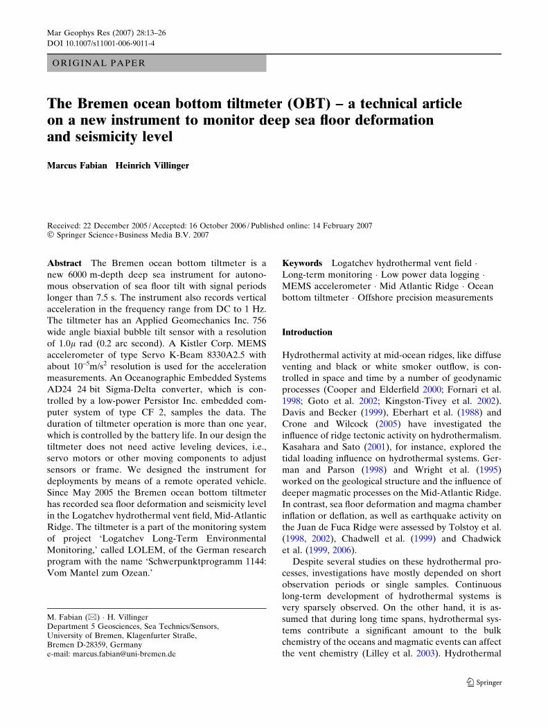
The model of the OBT shown in Fig. 1 gives an
overview of the instrument and its consistuent parts.
The aluminium frame consists of a triangular base
plate, a bar for handling and three legs with hollow
tips. An aluminium pressure case, which is screwed to
the base plate, houses the tilt and acceleration sensor.
The larger titanium case that lies horizontally in a
plastic tray contains the data logger, electronics and
batteries. Underwater connectors in the end caps of
both pressure cases feed the analog sensor signals from
the aluminium pressure case into the titanium case,
which houses the data logger. A newly developed
analogue deep sea level (Fabian and Heesemann 2006)
adjusts the instrument by means of an ROV.
Sensors
The OBT has two main sensors: A biaxial bubble tilt
sensor and an absolute accelerometer that has a re-
sponse curve starting from DC. In addition, a therm-
istor incorporated in the tilt sensor measures the
temperature inside the sensor pressure case, whereas
the bottom water temperature is recorded with a
miniaturized high-resolution (1 mK) temperature log-
ger (Pfender and Villinger 2002), which is lashed to the
frame of the OBT.
Tilt
We use an Applied Geomechanics Inc. (AGI) 756 wide
angle biaxial bubble tilt sensor with a resolution of
1.0l rad (0.2 arc second) and a repeatability of 2.0l rad
(AGI 2000). This type of sensor is known for its reli-
ability and long-term stability (d’Orey de Lantremange
1998; Mentes et al. 1996; Tofani and Horath 1990). The
comparatively broad effective range of ±8� is particu-
larly useful for our application. Hence, we do not need
to level the sensor (or the frame) very precisely when
installing it with an ROV on the sea floor.
Compared with data of Tolstoy et al. (1998, 2002),
who used a 0.05l rad resolution tilt sensor within an
OBS with a gimbal system, and assuming the same sea
floor conditions, we can clearly resolve long-term sig-
nals with high quality. Tolstoy et al. (1998) also report
tidal related tilts of amplitude below 1.0l rad. How-
ever, the signal strength depends on the sea floor
compliance and is position-dependent (Willoughby
et al. 2000; Crawford 2004; Hulme et al. 2005).
Therefore, we can not exclude the possibility that we
will observe tide-related tilt in the Logatchev hydro-
thermal vent field.
The tilt sensor electronics include a signal condi-
tioning card with two switchable gains of ratio 10
(high) to 1 (low) (AGI 2003). High gain amplifies small
tilt signals within a reduced effective range of ±0.8�.
For OBT operation we use the low gain setting and
feed the signals into a 24-bit data logger, so that a final
signal resolution of better than 1.0l rad is achieved.
+TY
+TX+AZ
aluminiumsensor pressure tube deep sea level
framedata loggerwith electronics
battery pack
sensor axesorientation
tripod with hollow profile
POM tray
titanium tube
Fig. 1 CAD-model of the OBT. Physical dimensions of the baseplate: 0.85 m (long edge) · [0.6 · 0.6 m]. Height of the OBT:0.45 m, weight in water: 450 N. Orientation of sensor axes, x-tilt,+TX, y-tilt, +TY and vertical acceleration, +AZ is shown
Mar Geophys Res (2007) 28:13–26 15
123

The signal conditioning card also has a built-in
switchable low-pass Butterworth filter with cut-off
periods of 0.05 s and 7.5 s both with 6 dB/octave roll-
off. For OBT operation we use the 7.5 s setting to re-
duce aliasing.
An other criterion for sensor selection is the power
consumption. Our AGI 756 with signal conditioning
card needs about 15 mA at ±12 V at an inclination
smaller than 2�. The AGI 756 also needs up to 27 mA
for larger angles in both axes. If the sensor is leveled
almost exactly then the required current drops to
11 mA. For autonomous long-term monitoring it is
desirable to reduce these values further in the future.
However, presently there are no sensors now on the
marked with similar resolution, repeatability, long-
term stability and significantly less power consumption
than the AGI 756.
Acceleration
For measurement of vertical acceleration we choose
the Kistler Servo K-Beam 8330A2.5 (Kistler 2004).
This is a MEMS class sensor, which is already used in
reflection seismic surveys (Byerley et al. 2003) and also
is suitable for seismological applications (Holland
2003). Micro-Electro-Mechanical Systems (MEMS)
integrate mechanical elements as well as sensor ele-
ments and electronics on a single small silicon wafer.
Similar to computer processor fabrication, the MEMS
sensor is fabricated through micro fabrication. Due to
the small size and high fabrication precision, these
sensors consume only a fraction of the power used by a
comparable classical sensor. Therefore, the MEMS
sensors noise level is relatively low and the resolution
as well as accuracy is quite high (Bernstein et al. 1999;
Hierold 2004; Moore and Syms 1999; Mougenot and
Thorburn 2004; Varadan 2000).
Nominal signal resolution of the Servo K-Beam is
close to 10–5m/s2 with a sensitivity of about 150 mV/
(m/s2). Frequency range is from DC to 300 Hz (reso-
nance frequency is 5000 Hz). To reject high frequency
components, which can not be sampled by our data
acquisition system due to power limitations, we con-
nected the output of the sensor to a passive low-pass
filter with 1 Hz corner frequency and a roll-off of
18 dB/decade.
As mentioned above, the strength of low frequency
background noise on the sea floor is in the same range
as the resolution of the Servo K-Beam (Crawford and
Webb 2000; Duennebier and Sutton 1995; Roman-
owicz et al. 1998; Zverev 1997), so that the sensor’s
resolution is sufficient for monitoring seismicity level.
For long-term deep sea measurements the MEMS
sensor has several advantages. Compared to a classical
seismograph these are small physical dimensions
(27 · 27 · 16 mm), operation without precise leveling,
relatively low power consumption (�17 mA, ±12 V),
robustness against mechanical shocks during transport
and deployment, low cost, light weight and easy han-
dling.
The Servo K-Beam works in any orientation. It
measures absolute acceleration in the direction of the
sensor axis (here in the vertical instrument axis of the
OBT). Because of this particular capability to measure
gravity, the combination of long-term acceleration and
tilt helps to verify long-term trends. Significant changes
in tilt have to be accompanied by a deviation of the
OBT, and as well by a comparable change in absolute
acceleration. On the other hand, with tilt data, vertical
acceleration can be corrected for deflections (Crawford
and Webb 2000).
Recently, Kistler Corporation has replaced the
Servo K-Beam 8330A2.5 by its successor the Servo K-
Beam 8330A3.0. With respect to the 8330A2.5, the
nominal noise density of the 8330A3.0 decreased by
50% and the nominal resolution is enhanced by the
same factor. The measuring range is 20% broader and
the sensitivity is reduced by about 20%. The temper-
ature coefficient has been increased by a factor of
nearly four. Minor modifications concern the fre-
quency range, resonant frequency and the phase-shift
(Kistler 2004, 2005). However, the test data we show in
section ‘Tests’ from both sensors, does not report large
differences between the sensors in practical operation.
Data logger and low power operation
The data logger has to fulfill several requirements,
which are (1) a suitable number of input channels with
a sufficiently high dynamic range and a sampling
interval small enough to resolve signals related to
seismicity, (2) storage capacity for at least one year of
data, (3) low power consumption and, (4) small size
and low cost. The battery capacity and the memory size
of the data logger have to be designed for a one year
long monitoring period at the sampling intervals de-
scribed below.
The Oceanographic Embedded Systems AD 24 24
bit AD-converter controlled by a Persistor Instruments
Inc. CF 2 (PersistorInc 2005) is a data logging system,
whose technical specifications meet our requirements.
The AD 24 is an add-on module that can be plugged in
the CF 2’s upgrade socket. The AD 24 implements two
Cirrus Logic Inc. CS 5534-BS 24 bit Sigma-Delta con-
verters, which provide four multiplexed input channels
each. Each of the channels can be configured freely.
16 Mar Geophys Res (2007) 28:13–26
123
The CF 2 is a Motorolla 68332 based embedded com-
puter system with 1 MB RAM and a slot for Com-
pactFlash cards. During logging, the RAM can be used
as a data buffer whose content is dumped to the
CompactFlash card when the buffer is full. The AD 24
board and CF 2 controller come with a suite of C-
libraries. Customers can incorporate functions of the
C-libraries in their own C-Code and build a customized
acquisition and processing software package.
The most important settings for an input channel of
the AD 24 are the conversion time, which is directly
related to the resolution, and the sampling period,
which has to be longer than the conversion time. At a
conversion time of 600 ms, a resolution of 22 effective
bits for an input signal of ±2.5 V can be achieved, but
the resolution depends somewhat on the individual
Sigma-Delta chip. Conversion time must be reduced, if
the sampling period is reduced to a time equal or
shorter than the conversion time. Accordingly, the
effective resolution is reduced. On the other hand, if
the highest resolution is not necessary (e.g., because of
limited sensor resolution), one can configure the cor-
responding channel to run at a shorter conversion time,
even if the sampling period is much longer. The
remaining time between sampling period and conver-
sion time can be used for dumping the content of the
data buffer from the RAM to the CompactFlash card,
or it can be used for switching the AD 24 and/or the CF
2 to its power saving mode. The latter is a very
advantageous setting for autonomous long-term oper-
ation.
In the standard OBT settings one channel is con-
figured to log the acceleration sensor output (i.e.,
output behind the low-pass filter) every 750 ms. To
achieve 21 effective bits resolution, which corresponds
to the sensors resolution, we set the conversion time to
300 ms. Therefore, every 750 ms, a period of 300 ms is
used to convert the acceleration values. The remaining
450 ms are used to sample tilt (x-tilt, y-tilt) and internal
temperature, to dump the data buffer to the Com-
pactFlash card, or to switch the data logger to sleep
mode. To determine both digital tilt values a 200 ms
conversion time, corresponding to 19 bit effective res-
olution, is used. A 30 ms conversion time, which cor-
responds to an effective resolution of 17 bit, is applied
for the internal temperature. Again, these settings
match the sensor’s dynamic ranges.
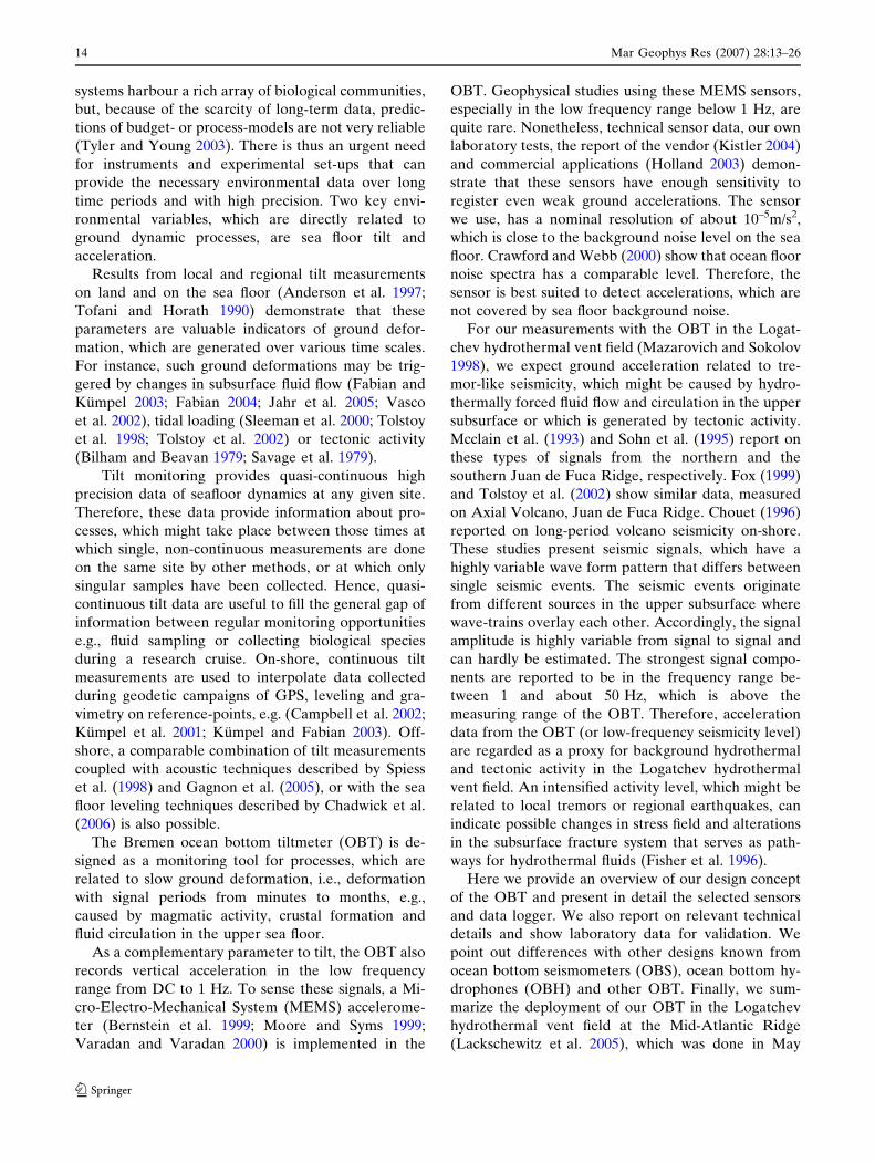
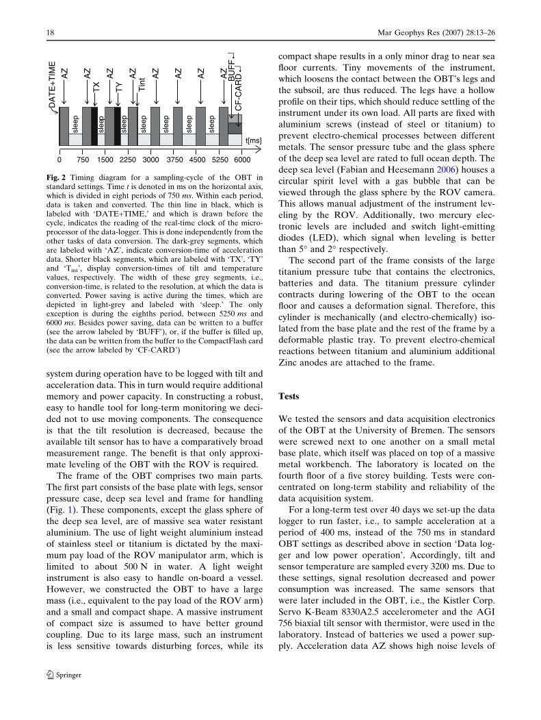
A timing diagram of one sampling cycle in standard
settings is shown in Fig. 2. The cycle is implemented in
the acquisition software as a loop. Eight individual
tasks of the data logger are executed in a sequence of
eight periods within this loop. Every task is controlled
by the real time clock of the CF 2. The clock is also
used to record a time stamp for the first data point of
every cycle. Clock drift measured during laboratory
tests with two different CF 2’s is about + 0.5 s/day at
room temperature (20–23�C). The time stamp is
determined at the beginning of every loop/sampling
cycle and parallel to the conversion of the first accel-
eration value. This moment is denoted by ‘DATE+-
TIME’ in Fig. 2. The eight individual tasks are: (1) take
acceleration data (AZ) – sleep (2) take acceleration
data (AZ) – take x-tilt data (TX) – sleep (3) take
acceleration data (AZ) – take y-tilt data (TY) – sleep
(4) take acceleration data (AZ) – take temperature
data (Tint) – sleep (5) take acceleration data (AZ) –
sleep (6) take acceleration data (AZ) – sleep (7) take
acceleration data (AZ) – sleep (8) take acceleration
data(AZ) – dump data to the buffer(BUFF)/Com-
pactFlash card(CF-CARD) or sleep. Because the
sampling period of acceleration data is 750 ms the loop
repeats every 6000 ms, which is the sampling period for
tilt and temperature data. The loop runs until the
CompactFlash card is full.
With these settings the data logger (AD 24 and CF
2) has a mean current consumption of 15 mA that is
independent from the operation voltage of the logger,
which should always be between 3.3 V and 15 V. For
power saving on the one hand and endurance of
operation on the other we chose a battery supply with
7.5 V output, deliberately not too close to the thresh-
old values.
At maximum inclination (‡ 8� in both directions TX,
TY) the maximum power consumption of all OBT
components is about 641 mW, which decreases to
497 mW at a mean inclination below 2� and is minimal
at 449 mW. With a safety factor of two the battery
pack of the OBT is budgeted to power the instrument
for 269 days (maximum power consumption), over
332 days (mean power consumption) to 367 days
(minimum power consumption). We use a 512 MB
CompactFlash card that can store data from more than
600 days of standard OBT operation.
Ground coupling, leveling devices and the frame
Good coupling of the sensor to the ground is very
important for tilt and low frequency acceleration
measurements (Agnew 1986). Therefore, there are no
moving parts between the sensors and the contact
points of the tripod on the ground. For platform tilt-
meters like the OBT, the best possible coupling should
be attained. A pure passive gimbal leveling system, for
instance, needs additional mechanical components,
which itself needs a thorough mechanical design and
testing procedure. Moreover, actions of the gimbal
Mar Geophys Res (2007) 28:13–26 17
123
system during operation have to be logged with tilt and
acceleration data. This in turn would require additional
memory and power capacity. In constructing a robust,
easy to handle tool for long-term monitoring we deci-
ded not to use moving components. The consequence
is that the tilt resolution is decreased, because the
available tilt sensor has to have a comparatively broad
measurement range. The benefit is that only approxi-
mate leveling of the OBT with the ROV is required.
The frame of the OBT comprises two main parts.
The first part consists of the base plate with legs, sensor
pressure case, deep sea level and frame for handling
(Fig. 1). These components, except the glass sphere of
the deep sea level, are of massive sea water resistant
aluminium. The use of light weight aluminium instead
of stainless steel or titanium is dictated by the maxi-
mum pay load of the ROV manipulator arm, which is
limited to about 500 N in water. A light weight
instrument is also easy to handle on-board a vessel.
However, we constructed the OBT to have a large
mass (i.e., equivalent to the pay load of the ROV arm)
and a small and compact shape. A massive instrument
of compact size is assumed to have better ground
coupling. Due to its large mass, such an instrument
is less sensitive towards disturbing forces, while its
compact shape results in a only minor drag to near sea
floor currents. Tiny movements of the instrument,
which loosens the contact between the OBT’s legs and
the subsoil, are thus reduced. The legs have a hollow
profile on their tips, which should reduce settling of the
instrument under its own load. All parts are fixed with
aluminium screws (instead of steel or titanium) to
prevent electro-chemical processes between different
metals. The sensor pressure tube and the glass sphere
of the deep sea level are rated to full ocean depth. The
deep sea level (Fabian and Heesemann 2006) houses a
circular spirit level with a gas bubble that can be
viewed through the glass sphere by the ROV camera.
This allows manual adjustment of the instrument lev-
eling by the ROV. Additionally, two mercury elec-
tronic levels are included and switch light-emitting
diodes (LED), which signal when leveling is better
than 5� and 2� respectively.
The second part of the frame consists of the large
titanium pressure tube that contains the electronics,
batteries and data. The titanium pressure cylinder
contracts during lowering of the OBT to the ocean
floor and causes a deformation signal. Therefore, this
cylinder is mechanically (and electro-chemically) iso-
lated from the base plate and the rest of the frame by a
deformable plastic tray. To prevent electro-chemical
reactions between titanium and aluminium additional
Zinc anodes are attached to the frame.
Tests
We tested the sensors and data acquisition electronics
of the OBT at the University of Bremen. The sensors
were screwed next to one another on a small metal
base plate, which itself was placed on top of a massive
metal workbench. The laboratory is located on the
fourth floor of a five storey building. Tests were con-
centrated on long-term stability and reliability of the
data acquisition system.
For a long-term test over 40 days we set-up the data
logger to run faster, i.e., to sample acceleration at a
period of 400 ms, instead of the 750 ms in standard
OBT settings as described above in section ‘Data log-
ger and low power operation’. Accordingly, tilt and
sensor temperature are sampled every 3200 ms. Due to
these settings, signal resolution decreased and power
consumption was increased. The same sensors that
were later included in the OBT, i.e., the Kistler Corp.
Servo K-Beam 8330A2.5 accelerometer and the AGI
756 biaxial tilt sensor with thermistor, were used in the
laboratory. Instead of batteries we used a power sup-
ply. Acceleration data AZ shows high noise levels of
AZ
TX
TY Tin
tAZ
AZ
AZ
DA
TE
+T
IME
AZ
AZ
AZ
AZ
CF
-CA
RDBU
FF
0 750 1500 2250 3000 3750 4500 5250 6000
t[ms]
slee
p
slee
p
slee
p
slee
p
slee
p
slee
p
slee
p
Fig. 2 Timing diagram for a sampling-cycle of the OBT instandard settings. Time t is denoted in ms on the horizontal axis,which is divided in eight periods of 750 ms. Within each period,data is taken and converted. The thin line in black, which islabeled with ‘DATE+TIME,’ and which is drawn before thecycle, indicates the reading of the real-time clock of the micro-processor of the data-logger. This is done independently from theother tasks of data conversion. The dark-grey segments, whichare labeled with ‘AZ’, indicate conversion-time of accelerationdata. Shorter black segments, which are labeled with ‘TX’, ‘TY’and ‘Tint’, display conversion-times of tilt and temperaturevalues, respectively. The width of these grey segments, i.e.,conversion-time, is related to the resolution, at which the data isconverted. Power saving is active during the times, which aredepicted in light-grey and labeled with ‘sleep.’ The onlyexception is during the eighths period, between 5250 ms and6000 ms. Besides power saving, data can be written to a buffer(see the arrow labeled by ‘BUFF’), or, if the buffer is filled up,the data can be written from the buffer to the CompactFlash card(see the arrow labeled by ‘CF-CARD’)
18 Mar Geophys Res (2007) 28:13–26
123

about 1 mm/s2, which is about to 50 times stronger than
the resolution of the acceleration measurements at the
conversion time of 200 ms. Compared to this, noise
level in tilt data TY, TX has an amplitude of about
10lrad, i.e., nearly five times the resolution, which can
be achieved at the used settings of 100 ms conversion
time.
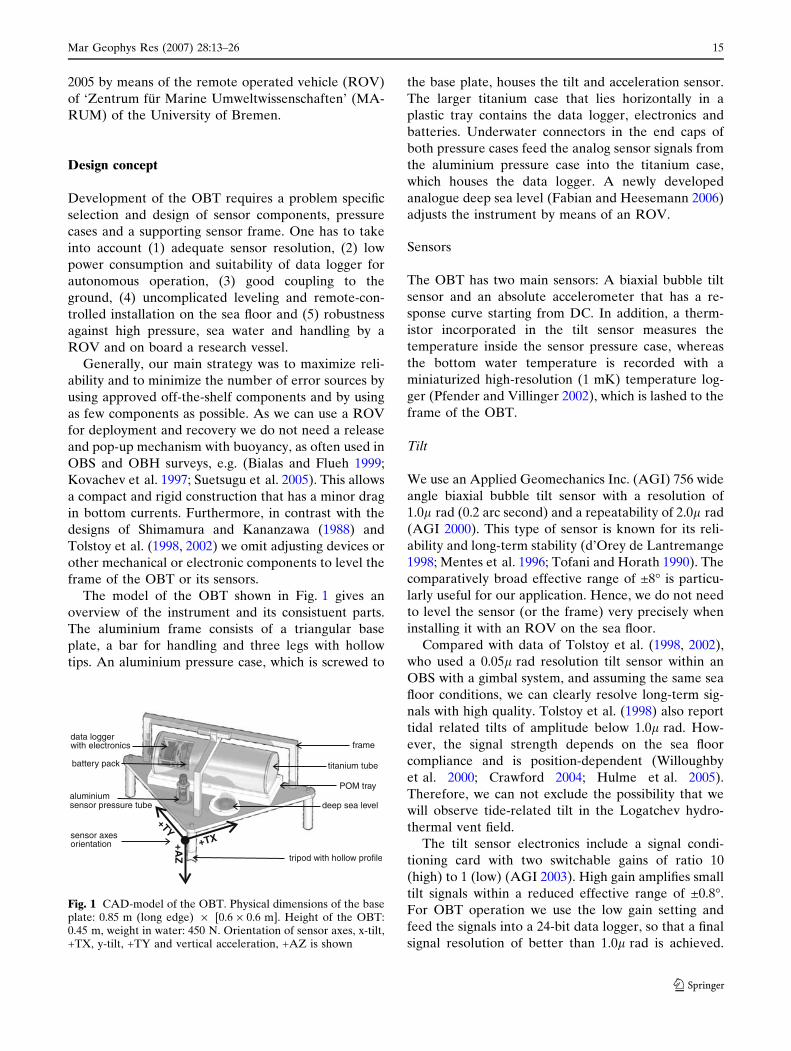
Figure 3 shows the data recorded from 15th
December 2004 to 24th January 2005. Measurements
were started on 14th December, but we excluded data
from the first 24 h, because there were disturbances in
the acceleration record, caused by laboratory work,
and a settling of about 95lrad in both tilt components.
The filtered time-series of acceleration data AZ shows
that spike-like events on 1st, 7th and 13th of January
are disturbances that contain only high frequencies.
Apart from the short period noise, the acceleration
signals strongly correlate with the internal sensor
temperature, Tint. In particular, during phases when
the temperature fluctuated strongly, e.g., on 15th, 16th,
21st, 24th, 25th, 29th December or during the 6th and
the 21st, 22nd and 23rd January the correlation be-
tween Tint and the vertical acceleration AZ is quite
strong. On 21st December this correlation was some-
what weak, and it reduced further on 11th and 12th
January. A very similar relation applies to the corre-
lation between the temperature and the tilt compo-
nents. However, this picture is not uniform. For
instance, on 17th, 18th, 22nd, 31st December and 4th,
7th, 10th, 12th, 15th and 17th January, the correlation
between both tilt-components and temperature is ra-
ther similar and strong. In contrast, on 16th, 24th, 25th,
December and on 19th January correlation with tem-
perature is significant, but quite different between both
tilt-components. A very similar correlation of acceler-
ation with temperature and tilt with temperature is
only recorded on 15th January. The reason for the
strong, but quite non-uniform influence of temperature
variations is most likely a complex expansion and
contraction of the metal constructions of sensors, the
metal base plate and the workbench.
Further remarkable features of Fig. 3 are noted on
the record for the 29th December, when an increase in
Tint seems to cause a jump in acceleration data AZ, but
could additionally be biased by a change in tilt TX and
TY. The strong jump in TX on the 6th January of
about 75lrad is accompanied by a very small change in
TY, which appears to be somewhat unusual, as well as
a stronger signal in AZ. Another similar jump in TX,
but about three times smaller, is seen on the 18th
January. Both signals are actually gradual changes over
a short time interval, but appear as jumps on the
compressed time scale of Fig. 3. Generally, the signal
of TY seems to be smoother than that from TX. In
other test configurations we checked both tilt compo-
nents, but could not determine a difference between
them. The long term change in temperature Tint be-
tween the 29th December and 24th January seems to
Fig. 3 Long-term test data over 40 days from December 15,2004 until January 24, 2005 and moving-window correlation withtemperature. From top to bottom the upper four time-seriesshow: original vertical acceleration AZ (Kistler Servo K-Beam8330A2.5) in light-grey, which is painted-over by filtered verticalacceleration in black (filter-frequency is 0.15 Hz). The diagram-panels below show the two perpendicular tilt components TYand TX and the sensor temperature, Tint (from AGI 756 biaxialtiltmeter with thermistor). Compare Fig. 1 for the sign andorientation of sensor axes to each other. The lower three time-series show moving-window calculations of the square of thecross-correlation between the sensor temperature Tint and theother data. Width of the moving-window is 24 h with a shift of1 h between two windows. Tint-AZ is the correlation between thesensor temperature and the filtered acceleration data, Tint-TYthe correlation with the Y-component of tilt, and Tint-TX thecorrelation with the X-component of tilt. On the whole, noiseoriginating from temperature variations and most likely causedby human activity dominates the data. Nonetheless, signals,which were caused by teleseismic waves of the M9.0 Sumatraearthquake of 26th December, with a epicentral distance of9527 km, appear in the time series of tilt and of acceleration (seealso the Fig. 4 that has an enlarged view on the signals from theseismic waves)
Mar Geophys Res (2007) 28:13–26 19
123

correlate quite well with the long term trend of TX and
TY. However, the accelerometer measures absolute
values, i.e., gravity, and all sensors are mounted on the
same base plate. Hence, the long-term change in TY of
about 250lrad over the complete time series might
cause the accompanying drop in acceleration values.
We note that there is no comparable change in the
temperature Tint, which starts and ends at about 22�C.
On the other hand, the strong long-period tilt variation
in TX between the 22nd and 29th December and
around the 17th January did not appear to be signifi-
cant in the acceleration data AZ.
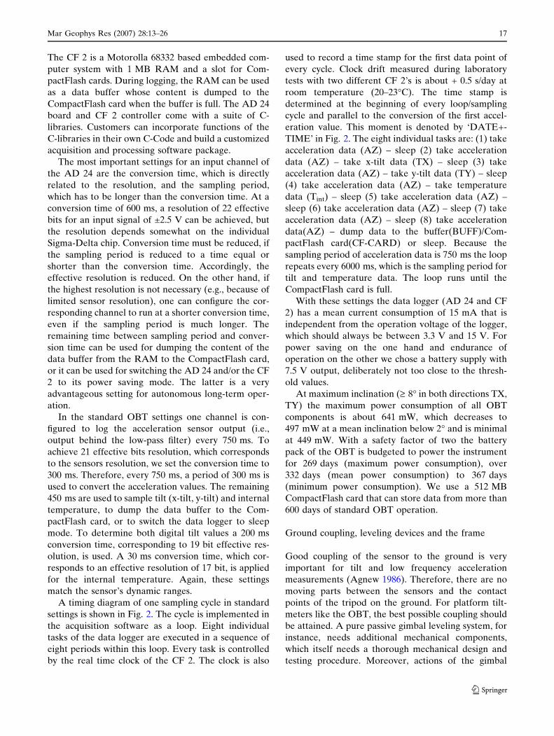
The teleseismic waves of the M9.0 Sumatra earth-
quake of 26th December are mostly buried in the
broad range of signals in Fig. 3 but cause a clear signal
in tilt and acceleration. Shaking of our institute build-
ing is clearly visible in tilt TX, TY, but acceleration
values also rise above the ambient noise level. Details
are shown in Fig. 4.
In Fig. 4 we smoothed the original acceleration data
with the same digital low-pass filter that was applied to
the data in Fig. 3 and that had a cut-off frequency of
0.15 Hz (6.67 s). Because of this data smoothing, noise
is reduced and the seismic waves (mostly the surface
waves that have their main frequency content below
0.15 Hz) appear quiet well. This proves that the Servo
K-Beam MEMS accelerometer is well suited to detect
motions in the frequency range between about 1 mHz
and 1 Hz, and especially in the frequency range of
teleseismic waves.
The amplitude spectra in the lower four panels of
Fig. 4 show significant frequency components in the
acceleration as well as the tilt registration. The stron-
gest frequency components, which are caused by
teleseismic waves, and which clearly correspond to the
spectrum calculated from the seismological data of Bad
Segeberg (BSEG-Z), are between 0.03 and 0.09 Hz.
The tilt spectra also correspond to the spectrum
BSEG-Z in the lower frequencies between about 0.017
and 0.03 Hz. These spectra (BSEG-Z, TY, TX) be-
come nearly flat in the frequency range down to
1 mHz. Spectra lines of the acceleration spectrum are
not so striking. The acceleration spectrum also shows
increasing components in the low frequency range
down to values of 1 mHz. Single spectra lines did not
correspond across all spectra. For instance, a spectra
line at 0.041 Hz in TY corresponds very well with the
spectra line in BSEG-Z, but it does not correspond
with the other spectra of AZ and TX. Different ori-
entation of the sensors in space may explain this dis-
crepancy.
During a second long-term test with a spare system
of the OBT’s sensors and data logger we recorded a
second teleseismic event. The logger was set up to run
in OBT standard mode (see section ‘Data logger and
low power operation’). As in the first test (Figs. 3, 4)
the recording system worked very reliable, in this case
for over two months, and produced time series of quite
similar quality. In this test we changed the acceler-
ometer type and tested the new Kistler Servo K-Beam
Fig. 4 Teleseismic waves of the M9.0 Sumatra earthquake ofDecember 26, 2004, 00:59 Universal Time Coordinated (UTC/GMT), and corresponding amplitude spectra. The signalsdenoted by AZ were recorded with a Kistler Servo K-Beam8330A2.5 accelerometer, and the signals denoted by TX, TY withan AGI 756 tilt sensor. Epicentral distance is 9527 km. To thecomparison we included between the records AZ and TY theuncalibrated record of the vertical component of the Germanseismological station in the town Bad Segeberg (Henger et al.2002), which is about 150 km northeast of our laboratory inBremen. This record is in grey. The p-wave arrivals are denotedby the arrow and PBESG. In all, the notation is the same as used inFig. 3. AZ shows the original data in light-gray; over-printeddata in black is filtered with a digital low-pass filter with 0.15 Hzcut-off frequency. Both TX and TY show original and unfiltereddata. The lower four panels of the diagram show the amplitudespectra. The spectra of the vertical acceleration AZ is calculatedfrom the filtered data
20 Mar Geophys Res (2007) 28:13–26
123

8330A3.0. The data shown in Fig. 5 confirms that this
new sensor is also appropriate for our application. The
teleseismic waves of the M7.6 Pakistan earthquake of
8th October 2005 (BGR 2004a) appear clearly. At a
first glance, wave form data from our sensors is not as
obvious as in Fig. 4. Inspected more precisely and
compared with the recordings of the seismological
station in Bad Segeberg (northern Germany; (Henger
et al. 2002)) the event becomes obvious. However,
energy release of this earthquake is several times
smaller than of the M9.0 Sumatra, even if epicentral
distance is roughly halved. For this test we used an-
other tilt sensor (but of the same AGI 756 type)
compared to the former test shown in Fig. 4. The dif-
ference in the noise level of tilt before and after the
teleseismic waves in Figs. 4 and 5 are due to the better
resolution of the data logger, which was switched to the
OBT standard mode.
The amplitude spectra of acceleration AZ and tilt
data TY, TX as well as of the seismological data from
Bad Segeberg, BSEG-Z are depicted in the lower four
panels of Fig. 5. Due to the lower sampling period
(6000 ms), the spectra of tilt data are limited to
0.083 Hz. Compared with the data shown in Fig. 4,
amplitudes of BSEG-Z are now nearly ten times
smaller and amplitudes of TY and TX are about five
times smaller. In both Figs. 4 and 5, the spectra of
acceleration data have the same scaling. In accordance
with the smaller energy release of the Pakistan earth-
quake, the frequency components in the spectrum of
acceleration are weak and significantly appear only
between 0.06 and 0.071 Hz. In the low frequencies
down to 1 mHz the spectrum does not show a gradual
increase of amplitudes, as seen in Fig. 4, but has some
relatively prominent lines, e.g., 0.01 or 0.0043 Hz. Due
to disturbances from the laboratory surroundings, high
frequency noise, which can be seen in the time series as
the broad grey band, is about 40% stronger than in
Fig. 4. Under these circumstances, it is hard to quan-
titatively compare both acceleration sensors, but we
can conclude that both are suited for the OBT.
A further demonstration of the capability and the
suitability of the OBT’s sensor system is shown in
Fig. 6. During a short term test of the measuring sys-
tem we observed seismic signals from a local earth-
quake. On October 20, 2004 a M4.5 local earthquake
occurred about 45 km southeast of Bremen. Source
time of the event was 06:59 Universal Time Coordi-
nated (UTC/GMT) (BGR 2004b). The earthquake had
an intensity of V+ on the European Macroseismic
Scale and was felt in the Bremen geoscience institute
building by some colleagues. In this case too, we used
the Kistler Servo K-Beam 8330A2.5 MEMS sensor to
measure vertical acceleration together with the AGI
756 tilt sensor, which were both used in the OBT. The
data logger was set-up to log each of the sensors with
the highest resolution, i.e. with a conversion time of
600 ms. Sampling interval was 8 s. The crosses on the
time series in Fig. 6a indicate single data points. The
tilt sensor clearly observed the shaking of the institute
building. Because the accelerometer output was logged
with the long sampling interval and because the local
earthquake did not generate a significant amount of
low-frequency accelerations, only a single pulse can be
seen in the corresponding data. The motion sequence
Fig. 5 Teleseismic waves of the M7.6 Pakistan earthquake ofOctober 8, 2005, 03:50 Universal Time Coordinated (UTC/GMT) (BGR 2004a), and corresponding amplitude spectra. Therepresentation is as in Fig. 4. Here, the signals denoted by AZwere recorded with a Kistler Servo K-Beam 8330A3.0 acceler-ometer, and the signals denoted by TX, TY with an AGI 756 tiltsensor. Epicentral distance is 5364 km. Again, for a betteridentification of the seismic waves we added (in grey) theuncalibrated record of the vertical component of the Germanseismological station in Bad Segeberg, which is about 150 kmnortheast of Bremen. The p-wave arrivals are denoted by anarrow and PBESG. TX and TY show original data
Mar Geophys Res (2007) 28:13–26 21
123
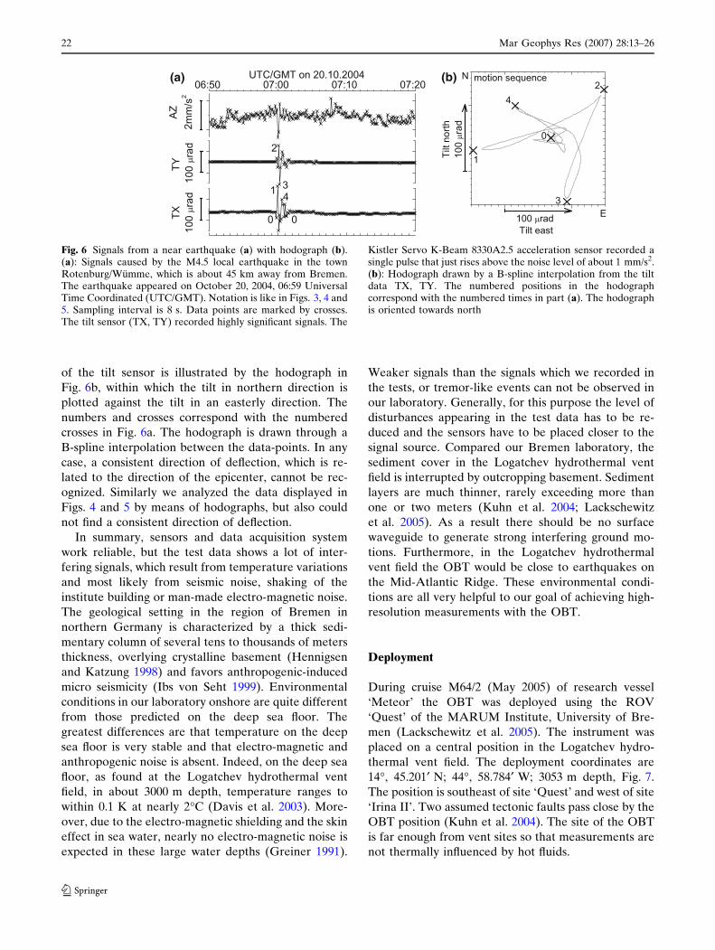
of the tilt sensor is illustrated by the hodograph in
Fig. 6b, within which the tilt in northern direction is
plotted against the tilt in an easterly direction. The
numbers and crosses correspond with the numbered
crosses in Fig. 6a. The hodograph is drawn through a
B-spline interpolation between the data-points. In any
case, a consistent direction of deflection, which is re-
lated to the direction of the epicenter, cannot be rec-
ognized. Similarly we analyzed the data displayed in
Figs. 4 and 5 by means of hodographs, but also could
not find a consistent direction of deflection.
In summary, sensors and data acquisition system
work reliable, but the test data shows a lot of inter-
fering signals, which result from temperature variations
and most likely from seismic noise, shaking of the
institute building or man-made electro-magnetic noise.
The geological setting in the region of Bremen in
northern Germany is characterized by a thick sedi-
mentary column of several tens to thousands of meters
thickness, overlying crystalline basement (Hennigsen
and Katzung 1998) and favors anthropogenic-induced
micro seismicity (Ibs von Seht 1999). Environmental
conditions in our laboratory onshore are quite different
from those predicted on the deep sea floor. The
greatest differences are that temperature on the deep
sea floor is very stable and that electro-magnetic and
anthropogenic noise is absent. Indeed, on the deep sea
floor, as found at the Logatchev hydrothermal vent
field, in about 3000 m depth, temperature ranges to
within 0.1 K at nearly 2�C (Davis et al. 2003). More-
over, due to the electro-magnetic shielding and the skin
effect in sea water, nearly no electro-magnetic noise is
expected in these large water depths (Greiner 1991).
Weaker signals than the signals which we recorded in
the tests, or tremor-like events can not be observed in
our laboratory. Generally, for this purpose the level of
disturbances appearing in the test data has to be re-
duced and the sensors have to be placed closer to the
signal source. Compared our Bremen laboratory, the
sediment cover in the Logatchev hydrothermal vent
field is interrupted by outcropping basement. Sediment
layers are much thinner, rarely exceeding more than
one or two meters (Kuhn et al. 2004; Lackschewitz
et al. 2005). As a result there should be no surface
waveguide to generate strong interfering ground mo-
tions. Furthermore, in the Logatchev hydrothermal
vent field the OBT would be close to earthquakes on
the Mid-Atlantic Ridge. These environmental condi-
tions are all very helpful to our goal of achieving high-
resolution measurements with the OBT.
Deployment
During cruise M64/2 (May 2005) of research vessel
‘Meteor’ the OBT was deployed using the ROV
‘Quest’ of the MARUM Institute, University of Bre-
men (Lackschewitz et al. 2005). The instrument was
placed on a central position in the Logatchev hydro-
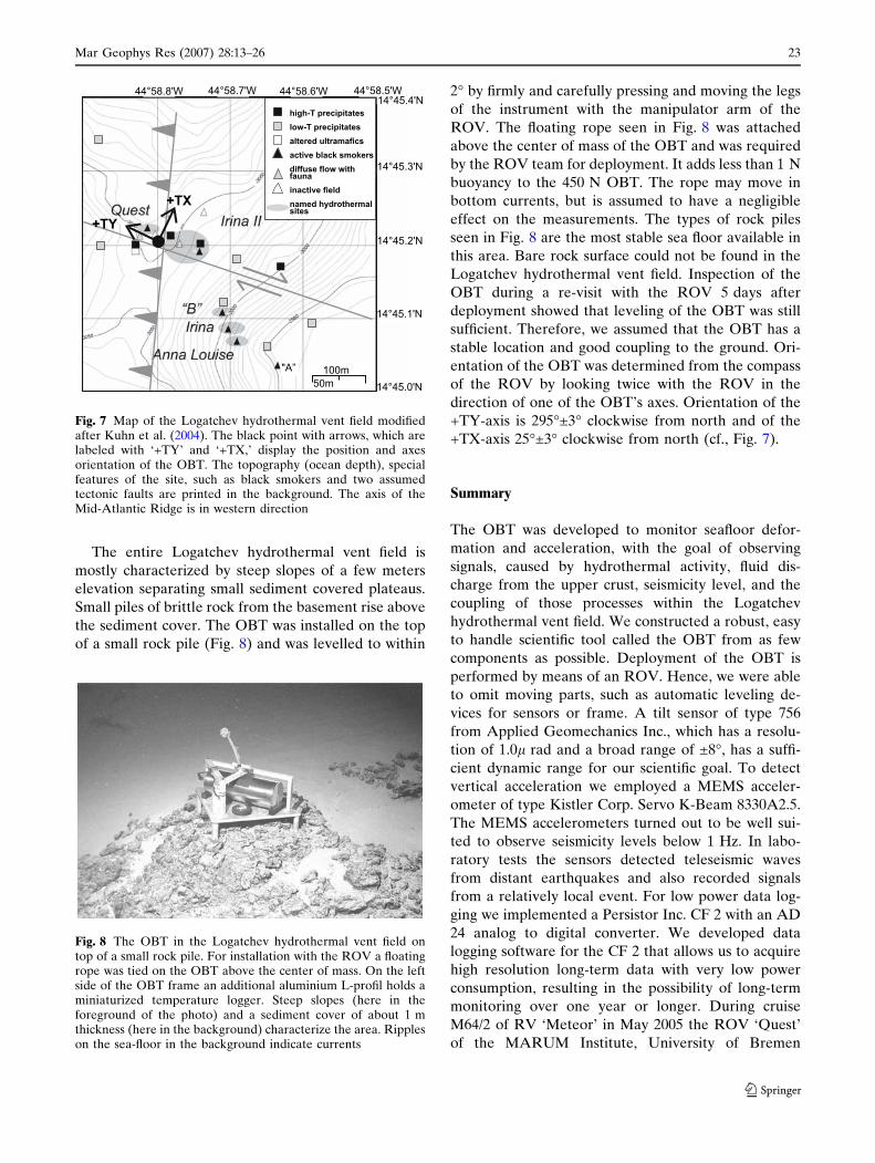
thermal vent field. The deployment coordinates are
14�, 45.201¢ N; 44�, 58.784¢ W; 3053 m depth, Fig. 7.
The position is southeast of site ‘Quest’ and west of site
‘Irina II’. Two assumed tectonic faults pass close by the
OBT position (Kuhn et al. 2004). The site of the OBT
is far enough from vent sites so that measurements are
not thermally influenced by hot fluids.
(b)(a)
Fig. 6 Signals from a near earthquake (a) with hodograph (b).(a): Signals caused by the M4.5 local earthquake in the townRotenburg/Wumme, which is about 45 km away from Bremen.The earthquake appeared on October 20, 2004, 06:59 UniversalTime Coordinated (UTC/GMT). Notation is like in Figs. 3, 4 and5. Sampling interval is 8 s. Data points are marked by crosses.The tilt sensor (TX, TY) recorded highly significant signals. The
Kistler Servo K-Beam 8330A2.5 acceleration sensor recorded asingle pulse that just rises above the noise level of about 1 mm/s2.(b): Hodograph drawn by a B-spline interpolation from the tiltdata TX, TY. The numbered positions in the hodographcorrespond with the numbered times in part (a). The hodographis oriented towards north
22 Mar Geophys Res (2007) 28:13–26
123
The entire Logatchev hydrothermal vent field is
mostly characterized by steep slopes of a few meters
elevation separating small sediment covered plateaus.
Small piles of brittle rock from the basement rise above
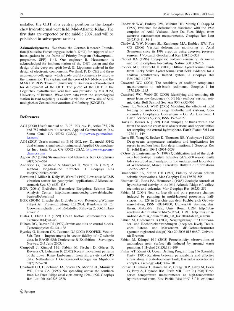
the sediment cover. The OBT was installed on the top
of a small rock pile (Fig. 8) and was levelled to within
2� by firmly and carefully pressing and moving the legs
of the instrument with the manipulator arm of the
ROV. The floating rope seen in Fig. 8 was attached
above the center of mass of the OBT and was required
by the ROV team for deployment. It adds less than 1 N
buoyancy to the 450 N OBT. The rope may move in
bottom currents, but is assumed to have a negligible
effect on the measurements. The types of rock piles
seen in Fig. 8 are the most stable sea floor available in
this area. Bare rock surface could not be found in the
Logatchev hydrothermal vent field. Inspection of the
OBT during a re-visit with the ROV 5 days after
deployment showed that leveling of the OBT was still
sufficient. Therefore, we assumed that the OBT has a
stable location and good coupling to the ground. Ori-
entation of the OBT was determined from the compass
of the ROV by looking twice with the ROV in the
direction of one of the OBT’s axes. Orientation of the
+TY-axis is 295�±3� clockwise from north and of the
+TX-axis 25�±3� clockwise from north (cf., Fig. 7).
Summary
The OBT was developed to monitor seafloor defor-
mation and acceleration, with the goal of observing
signals, caused by hydrothermal activity, fluid dis-
charge from the upper crust, seismicity level, and the
coupling of those processes within the Logatchev
hydrothermal vent field. We constructed a robust, easy
to handle scientific tool called the OBT from as few
components as possible. Deployment of the OBT is
performed by means of an ROV. Hence, we were able
to omit moving parts, such as automatic leveling de-
vices for sensors or frame. A tilt sensor of type 756
from Applied Geomechanics Inc., which has a resolu-
tion of 1.0l rad and a broad range of ±8�, has a suffi-
cient dynamic range for our scientific goal. To detect
vertical acceleration we employed a MEMS acceler-
ometer of type Kistler Corp. Servo K-Beam 8330A2.5.
The MEMS accelerometers turned out to be well sui-
ted to observe seismicity levels below 1 Hz. In labo-
ratory tests the sensors detected teleseismic waves
from distant earthquakes and also recorded signals
from a relatively local event. For low power data log-
ging we implemented a Persistor Inc. CF 2 with an AD
24 analog to digital converter. We developed data
logging software for the CF 2 that allows us to acquire
high resolution long-term data with very low power
consumption, resulting in the possibility of long-term
monitoring over one year or longer. During cruise
M64/2 of RV ‘Meteor’ in May 2005 the ROV ‘Quest’
of the MARUM Institute, University of Bremen
+TY
+TX
high-T precipitates
low-T precipitates
altered ultramafics
active black smokers
diffuse flow withfauna
inactive field
named hydrothermalsites
44°58.8'W 44°58.7'W 44°58.6'W 44°58.5'W
14°45.0'N
14°45.1'N
14°45.2'N
14°45.3'N
14°45.4'N
"A” 100m
50m
Fig. 7 Map of the Logatchev hydrothermal vent field modifiedafter Kuhn et al. (2004). The black point with arrows, which arelabeled with ‘+TY’ and ‘+TX,’ display the position and axesorientation of the OBT. The topography (ocean depth), specialfeatures of the site, such as black smokers and two assumedtectonic faults are printed in the background. The axis of theMid-Atlantic Ridge is in western direction
Fig. 8 The OBT in the Logatchev hydrothermal vent field ontop of a small rock pile. For installation with the ROV a floatingrope was tied on the OBT above the center of mass. On the leftside of the OBT frame an additional aluminium L-profil holds aminiaturized temperature logger. Steep slopes (here in theforeground of the photo) and a sediment cover of about 1 mthickness (here in the background) characterize the area. Rippleson the sea-floor in the background indicate currents
Mar Geophys Res (2007) 28:13–26 23
123
installed the OBT at a central position in the Logat-
chev hydrothermal vent field, Mid-Atlantic Ridge. The
first data are expected by the middle 2007, and will be
published in subsequent articles.
Acknowledgements We thank the German Research Founda-tion (Deutsche Forschungsgesellschaft, DFG) for support of ourinvestigations in the frame of Priority Program (Schwerpunkt-programm, SPP) 1144. Our engineer B. Heesemann isacknowledged for implementation of the OBT design and thedesign of the deep sea spirit level. E. Lippmann assisted in thedesign of electronic components. We thank P. D. Clift and threeanonymous colleagues, which made useful comments to improvethe manuscript. The captain and the crew of RV Meteor and theMARUM ROV Team of University of Bremen is acknowledgedfor deployment of the OBT. The photo of the OBT in theLogatchev hydrothermal vent field was provided by MARUM,University of Bremen. Wave form data from the seismologicalstation in Bad Segeberg is available via the WWW-site of Seis-mologisches Zentralobservatorium Grafenberg (SZGRF).
References
AGI (2000) User’s manual no. B-92-1003, rev. B., series 755, 756and 757 miniature tilt sensors, Applied Geomechanics Inc.,Santa Cruz, CA 95062 (USA), http://www.geomechan-ics.com/
AGI (2003) User’s manual no. B-92-1002, rev. D., model 83162dual-channel signal conditioning card, Applied Geomechan-ics Inc., Santa Cruz, CA 95062 (USA), http://www.geome-chanics.com/
Agnew DC (1986) Strainmeters and tiltmeters. Rev Geophysics24(3):579–624
Anderson G, Constable S, Staudigel H, Wyatt FK (1997) Aseafloor long-baseline tiltmeter. J Geophys Res102(B9):20269–20285
Bernstein J, Miller R, Kelly W, Ward P (1999) Low-noise MEMSvibration sensor for geophysical applications. J Microelec-tromech Syst 8(4):433–438
BGR (2004a) Erdbeben, Besondere Ereignisse, Seismic DataAnalysis Center, http://sdac.hannover.bgr.de/web/sdac/be-ben/erdbeben.html
BGR (2004b) Ursache des Erdbebens von Rotenburg/Wummeaufgeklart, Pressemitteilung 3.12.2004, Bundesanstalt furGeowissenschaften und Rohstoffe, Stilleweg 2, 30655 Han-nover: 2
Bialas J, Flueh ER (1999) Ocean bottom seismometers. SeaTechnol 40(4):41–46
Bilham RG, Beavan RJ (1979) Strains and tilts on crustal blocks.Tectonophysics 52:121–138
Byerley G, Klausen CK, Tessman DJ (2003) EKOFISK Vector-Seis Test – Improvements in vector fidelity of 4C seismicdata. In EAGE 65th Conference & Exhibition – Stavanger,Norway, 2–5 June 2003, 4
Campbell J, Kumpel H-J, Fabian M, Fischer D, Gorres B,Keysers CJ, Lehmann K (2002) Recent movement patternsof the Lower Rhine Embayment from tilt, gravity and GPSdata. Netherlands J Geosciences/Geologie en Mijnbouw81(2):223–230
Chadwell CD, Hildebrand JA, Spiess FN, Morton JL, MormarkWR, Reiss CA (1999) No spreading across the southernJuan De Fuca Ridge axial cleft during 1994–1996. GeophysRes Lett 26(16):2525–2528
Chadwick WW, Embley RW, Milburn HB, Meinig C, Stapp M(1999) Evidence for deformation associated with the 1998eruption of Axial Volcano, Juan De Fuca Ridge, fromacoustic extensometer measurements. Geophys Res Lett26(23):3441–3444
Chadwick WW, Nooner SL, Zumberge MA, Embley RW, FoxCG (2006) Vertical deformation monitoring at AxialSeamount since its 1998 eruption using deep-sea pressuresensors. J Volcanol Geothermal Res 150:313–327
Chouet BA (1996) Long-period volcano seismicity: its sourceand use in eruption forecasting. Nature 380:309–316
Cooper MJ, Elderfield H (2000) Diffuse hydrothermal fluidsfrom Lucky Strike hydrothermal vent field: evidence for ashallow conductively heated system. J Geophys ResB8:19369–19375
Crawford WC (2004) The sensitivity of seafloor compliancemeasurements to sub-basalt sediments. Geophys J Int157:1130–1145
Crawford WC, Webb SC (2000) Identifying and removing tiltnoise from low-frequency (< 0.1 Hz) seafloor vertical seis-mic data. Bull Seismol Soc Am 90(4):952–963
Crone TJ, Wilcock WSD (2005) Modeling the effects of tidalloading on mid-ocean ridge hydrothermal systems, Geo-chemistry Geophysics Geosystems – G3. An Electronic JEarth Sciences 6(7):25, ISSN 1525–2027
Davis E, Becker K (1999) Tidal pumping of fluids within andfrom the oceanic crust: new observations and opportunitiesfor sampling the crustal hydrosphere. Earth Planet Sci Lett172:141–149
Davis EE, Wang K, Becker K, Thomson RE, Yashayaev I (2003)Deep-ocean temperature variations and implications forerrors in seafloor heat flow determinations. J Geophys ResB: Solid Earth 108(1):2034–2039
d’Orey de Lantremange N (1998) Qualification test of the dual-axis bubble-type resistive tiltmeter (AGI-700 series): earthtides recorded and analyzed in the underground laboratoryof Walferdange, Maree Terrestres. Bulletin d’Informations129:9953–9962
Duennebier FK, Sutton GH (1995) Fidelity of ocean bottomseismic observations. Mar Geophys Res 17:535–555
Eberhart GL, Rona PA, Honnorez J (1988) Geologic controls ofhydrothermal activity in the Mid-Atlantic Ridge rift valley:tectonics and volcanics. Mar Geophys Res 10:233–259
Fabian M (2004) Near surface tilt and pore pressure changesinduced by pumping in multi-layered poroelastic half-spaces, no. 229 in Berichte aus dem Fachbereich Geowis-senschaften, ISSN: 0931-0800, Universitat Bremen, diss.thesis, Math.-Nat. Fak., Univ. Bonn, URN: http://nbn-resolving.de/urn:nbn:de:hbz:5-03724, URL: http://hss.ulb.u-ni-bonn.de/diss_online/math_nat_fak/2004/fabian_marcus
Fabian M, Heesemann B (2006) Neigungswaage fur Unterwas-ser- und Hochdruckanwendungen (deep sea level), Deuts-ches Patent- und Markenamt, dE-Gebrauchsmuster(german registered design) Nr.: 20 2006 013 066.7, Univers-tat Bremen
Fabian M, Kumpel H-J (2003) Poroelasticity: observations ofanomalous near surface tilt induced by ground waterpumping. J Hydrol 281(3):191–209
Fisher AT, Zwart G, Ocean Drilling Program Leg 156 ScientificParty (1996) Relation between permeability and effectivestress along a plate-boundary fault, Barbados accretionarycomplex. Geology 24(4):307–310
Fornari DJ, Shank T, Damm KLV, Gregg TKP, Lilley M, LevaiG, Bray A, Haymon RM, Perfit MR, Lutz R (1998) Time-series temperature measurements at high-temperaturehydrothermal vents, East Pacific Rise 9�49¢–51¢ N: evidence
24 Mar Geophys Res (2007) 28:13–26
123

for monitoring a crustal cracking event. Earth Planet SciLett 160:419–431
Fox CG (1999) In situ ground deformation measurements fromthe summit of Axial Volcano during the 1998 volcanicepisode. Geophys Res Lett 26(23):3437–3440
Gagnon K, Chadwell D, Spiess FN (2005) Evolving method tomeasure seafloor plate tectonic motions. Sea Technol46(7):49–52
German CR, Parson LM (1998) Distributions of hydrothermalactivity along the Mid-Atlantic Ridge: interplay of mag-matic and tectonic controls. Earth Planet Sci Lett 160:327–341
Goto S, Kinoshita M, Matsubayashi O, Von Herzen RP (2002)Geothermal constrains on the hydrological regime of theTAG active hydrothermal mound, inferred from long-termmonitoring. Earth Planet Sci Lett 203:149–163
Greiner W (1991) Klassische Elektrodynamik, TheoretischePhysik, Band 3, Verlag Harri Deutsch, Frankfurt a.M., Thun
Henger M, Berckhemer H, Seidl D (2002) The history of thedevelopment of the German Regional Seismic Network(GRSN). In Korn M (ed) Ten years of German RegionalSeismic Network (GRSN), ISBN 3-527-27514-2, 1–8
Hennigsen D, Katzung G (1998) Einfuhrung in die GeologieDeutschlands, Enke-Verlag, Stuttgart, 5th edn
Hierold C (2004) From micro- to nanosystems: mechanicalsensors go nano. J Micromech Microeng 14:S1–S11
Holland A (2003) Earthquake data recorded by the MEMSaccelerometer: field testing in Idaho. Seismol Res Lett Lett74(1):20–26
Hulme T, Crawford WC, Singh SC (2005) The sensitivity ofseafloor compliance to two-dimensional low-velocity anom-alies. Geophys J Int 163:547–558
Ibs von Seht M (1999) Microtremor measurements used to mapthickness of soft sediments. Bull Seismol Soc Am 89(1):250–259
Jahr T, Jentzsch G, Letz H, Sauter M (2005) Fluid injection andsurface deformation at the KTB location: modelling ofexpected tilt effects. Geofluids 5(1):20
Kasahara J, Sato T (2001) Tidal effect on volcanic earthquakesand deep-sea hydrothermal activity revealed by oceanbottom seismometer measurements. J Geodetic Soc Japan47(1):424–433
Kingston-Tivey M, Bradley AM, Joyce TM, Kadko D (2002)Insights into tide-related variability at seafloor hydrother-mal vents from time-series temperature measurements.Earth Planet Sci Lett 202:693–707
Kistler (2004) Operating instructions K-Beam & ServoK-Beamcapacitive accelerometers types 8304B(X), 8305A(X),8310A(X)M11, 8312A(X), 8330A2.5, 8392B(X), 8393A(X),Kistler Instrument Corp., 75 John Glenn Drive, Amherst,NY 14228, USA. http://www.kistler.com/
Kistler (2005) Operating instructions K-Beam & ServoK-Beamcapacitive accelerometers types 8304B(X), 8305A(X),8310A(X)M11, 8312A(X), 8330(X), 8392B(X), 8393A(X),Kistler Instrument Corp., 75 John Glenn Drive, Amherst,NY 14228, USA. http://www.kistler.com/
Kovachev SA, Demidova TA, Son’kin A (1997) Properties ofnoise registered by pop-up ocean-bottom seismographs. JAtmos Oceanic Technol 14(4):883–888
Kuhn T, Alexander B, Augustin N, Birgel D, Borowski C, deCarvalho LM, Engemann G, Ertl S, Franz L, Grech C,Hekinian R, Imhoff J, Jellinek T, Klar S, Koschinsky A,Kuever J, Kulescha F, Lackschewitz K, Petersen S,Ratmeyer V, Renken J, Ruhland G, Scholten J, SchreiberK, Turkay M, Westernstroer U, Zielinski F (2004)Mineralogical, geochemical and biological investigations of
hydrothermal systems on the Mid-Atlantic Ridge between14�45¢ N and 15�05¢ N (HYDROMAR I), Meteor Berichte03-04, Mid-Atlantic Expedition 2004, Cruise No. 60, Leg 3,Leitstelle Meteor, Institut fur Meereskunde der UniversitatHamburg
Kumpel H-J, Fabian M (2003) Tilt monitoring to assess thestability of geodetic reference points in permafrost environ-ment. Phys Chem Earth 28:1249–1256
Kumpel H-J, Lehmann K, Fabian M, Mentes G (2001) Pointstability at shallow depth – experience from tilt measure-ments in the Lower Rhine Embayment, Germany, andimplications for high resolution GPS and gravity recordings.Geophys J Int 146:699–713
Lackschewitz K, Armini M, Augustin N, Dubilier N, Edge D,Engemann G, Fabian M, Felden J, Franke P, Gartner A,Garbe-Schonberg D, Gennerich H-H, Huttig D, MarblerH, Meyerdierks A, Pape T, Perner M, Reuter M, RuhlandG, Schmidt K, Schott T, Schroeder M, Schroll G, Seiter C,Stecher J, Strauss H, Viehweger M, Weber S, WenzhoferF, Zielinski F (2005) Longterm study of hydrothermalismand biology at the Logatchev field, Mid-Atlantic Ridge at15�N (revisit 2005) (HYDROMAR II), Meteor Berichte05, Mid-Atlantic Expedition 2005, Cruise No. 64, Leg 2,Leitstelle Meteor, Institut fur Meereskunde der UniversitatHamburg, 6 May–6 June 2005, Fortaleza (Brazil) – Dakar(Senegal)
Lilley MD, Butterfield DA, Lupton JE, Olson EJ (2003)Magmatic events can produce rapid changes in hydrother-mal vent chemistry. Nature 422:878–881
Mazarovich AO, Sokolov S (1998) The tectonic position ofhydrothermal fields on the Mid-Atlantic Ridge. LitholMineral Res 33(4):391–394
McClain JS, Begnaud ML, Wright MA, Fondrk J, Damm GKV(1993) Seismicity and tremor in a submarine hydrothermalfield: the northern Juan De Fuca Ridge. Geophys Res Lett20(17):1883–1886
Mentes G, Lehmann K, Varga P, Kumpel H-J (1996) Somecalibration of the Applied Geomecanics Inc. boreholetiltmeter model 722. Acta Geodaetica et Geophysica Hun-garica 31:79–89
Moore DF, Syms RRA (1999) Recent developments in mi-cromachined silicon. Electron Commun Eng J 11(6):261–270
Mougenot D, Thorburn N (2004) MEMS-based 3C accelerom-eters for land seismic acquisition: Is it time? The LeadingEdge 23(3):246–250
PersistorInc (2005) Persistor Instruments Inc., Persistor Instru-ments Inc., 254-J Shore Rd, Bourne MA 02532-4104, USA,http://www.persistor.com/
Pfender M, Villinger H (2002) Miniaturized data loggers fordeep sea sediment temperature gradient measurements.Mar Geol 186:557–570
Romanowicz B, Stakes D, Montagner JP, Tarits P, UhrhammerR, Begnaud M, Stutzmann E, Pasyanos M, Karczewski J-F,Etchemendy S, Neuhauser D (1998) MOISE: a pilotexperiment towards long term sea-floor geophysical obser-vatories. Earth Planets Space 50(11–12):927–937
Savage JC, Prescott WH, Chamberlain JF, Lisowski M, Morten-sen CE (1979) Geodetic tilt measurements along the SanAndreas Fault in central California. Bull Seismol Soc Am69(6):1965–1981
Shimamura H, Kanazawa T (1988) Ocean bottom tiltmeter withacoustic data retrival system implated by a submersible. MarGeophys Res 9:237–254
Sleeman R, Haak HW, Bos MS, van Gend JJA (2000) Tidal tiltobservations in the Netherlands using shallow boreholetiltmeters. Phys Chem Earth (A) 25:415–420
Mar Geophys Res (2007) 28:13–26 25
123

Sohn RA, Hildebrand JA, Webb SC, Fox CG (1995) Hydro-thermal microseismicity at the meagaplume site on thesouthern Juan de Fuca Ridge. Bull Seismol Soc Am85(3):775–786
Spiess FN, Chadwell CD, Hildebrand JA, Young LE Jr, PurcellGH, Dragert H (1998) Precise GPS/Acoustic positioning ofseafloor reference points for tectonic studies. Phys EarthPlanet Interiors 108:101–112
Suetsugu D, Shiobara H, Sugioka H, Barruol G, Schindele F,Reymond D, Bonneville A, Debayle E, Isse T, Kanazawa T,Fukao Y (2005) Probing south Pacific Mantle Plumes withocean bottom seismographs, EOS, Transactions. Am Geo-phys Union 86(44):429, 435
Tofani G, Horath F (1990) Continuous tiltmeter monitoring toidentify ground deformation mechanisms. Geotech News8(2):31–35
Tolstoy M, Constable S, Orcutt JA, Staudigel H, Wyatt FK,Anderson G (1998) Short and long baseline tiltmetermeasurements on axial seamount, Juan de Fuca Ridge.Phys Earth Planet Interiors 108:129–141
Tolstoy M, Vernon FL, Orcutt JA, Wyatt FK (2002) Breathingof the seafloor: tidal correlations of seismicity at Axialvolcano. Geology 30(6):503–506
Tyler PA, Young CM (2003) Dispersal at hydrothermal vents: asummary of recent progress. Hydrobiologia 503:9–19
Varadan VK, Varadan VV (2000) Microsensors, microelectro-mechanical systems (MEMS), and electronics for smartstructures and systems. Smart Mater Struct 9:953–972
Vasco DW, Karasaki K, Nakagome O (2002) Monitoringreservoir production using surface deformation at theHijiori test site and the Okuaizu geothermal field, Japan.Geothermics 31(3):303–342
Willoughby EC, Letychev K, Edwards RN, Mihajlovic G(2000) Resource evaluation of marine gas hydrate depositsusing seafloor compliance methods. Annals NY Acad Sci912:146–158
Wright DJ, Haymon RM, Fornari DJ (1995) Crustal fissuring andits relationship to magmatic and hydrothermal processes onthe East Pacific Rise crest (9�12¢ to 54¢ N). J Geophys Res100(B4):6097–6120
Zverev SM (1997) Ocean-floor noise monitoring in the SouthAtlantic. Volcanol Seismol 18:703–730
26 Mar Geophys Res (2007) 28:13–26
123
Top Related