


Languages
Pages
Legal

Text Mining: Approaches and ApplicationsText Mining: Approaches and Applications
Claim Severity Case StudyClaim Severity Case Study
2011 SOA Health Meeting 2011 SOA Health Meeting
Session 61Session 61
Jonathan Polon FSAwww.claimanalytics.com

2
Agenda
Text Mining for Health Insurers
Case Study
Overview
Text Mining
Results
Questions

Text MiningFor
Health Insurers
4
Text Mining for Health Insurance
• Risk Measurement• Underwriting• Pricing
• Claims Management• Fraud detection• Claim approval• Case management
4

5
Sources of Text
• Application Process• Application for insurance• Attending physician statements• Call center logs
• Post Claim• Claim application• Attending physician statements• Adjuster notes• Call center logs• Other correspondence
5

6
Why Use Text Mining?
• May contain information not available in structured data fields
• May contain subjective data (eg, expert opinions)
• May be an early indicator of severity
– Lags in receiving treatment
– Lags in receiving and processing bills
6

7
Case StudyOverview
8
Project Overview
• Workers compensation business
• Medical only claims
• 15 days from First Notice on Loss (FNOL)
• For each claim predict likelihood that Total Claim Cost will exceed a specified threshold
8

9
Data Sources
9

10
Case StudyText Mining

11
Modeling Approach
1. Exploratory stage:
a. Train models without any text mining
b. Train models exclusively with text mining
2. Intermediate stage:
a. Apply text mining to predict residuals of non-text model
3. Final model:
a. Combine text and non-text predictors using the findings from Steps 1a and 2a
11

12
Text Mining Considerations
1. Word frequencies
2. Stemming
3. Exclusion list
4. Phrases
5. Synonyms
6. Negatives
7. Singular value decomposition
12
13
1. Word Frequencies
• Text mining for predictive modeling:– Identify words or phrases that occur frequently within the text
– Test to see if any of these words or phrases are predictive of the event being modeled
– Typically limit analysis to words whose frequency in the text exceeds a minimum amount (eg, is contained in at least 3% of all records)
13
14
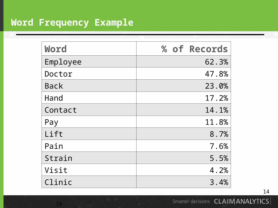
Word Frequency Example
Word % of RecordsEmployee 62.3%
Doctor 47.8%
Back 23.0%
Hand 17.2%
Contact 14.1%
Pay 11.8%
Lift 8.7%
Pain 7.6%
Strain 5.5%
Visit 4.2%
Clinic 3.4%
14

15
2. Stemming
• Reduce words to their roots so that related words are treated as the same
• For example:
– Investigate, investigated, investigation, investigator
– Can all be stemmed to investigat and treated as the same word
15
16
3. Exclusion List
• Common words that carry little meaning can be defined and excluded from the text mining analysis
• For example: the, of, and are unlikely to provide predictive value
16
17
4. Phrases
• Common phrases may be pre-specified by the user to consider as one string
– Eg, lower back, lost time
• N-grams: count frequency of every combination of N consecutive words
– May be more effective to identify groups of words that appear together frequently even if not consecutively
17
18
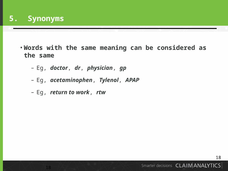
5. Synonyms
• Words with the same meaning can be considered as the same
– Eg, doctor, dr, physician, gp
– Eg, acetaminophen, Tylenol, APAP
– Eg, return to work, rtw
18
19
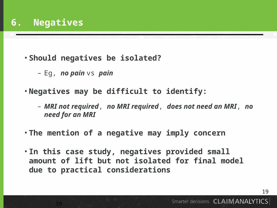
6. Negatives
• Should negatives be isolated?
– Eg, no pain vs pain
• Negatives may be difficult to identify:
– MRI not required, no MRI required, does not need an MRI, no need for an MRI
• The mention of a negative may imply concern
• In this case study, negatives provided small amount of lift but not isolated for final model due to practical considerations
19
20
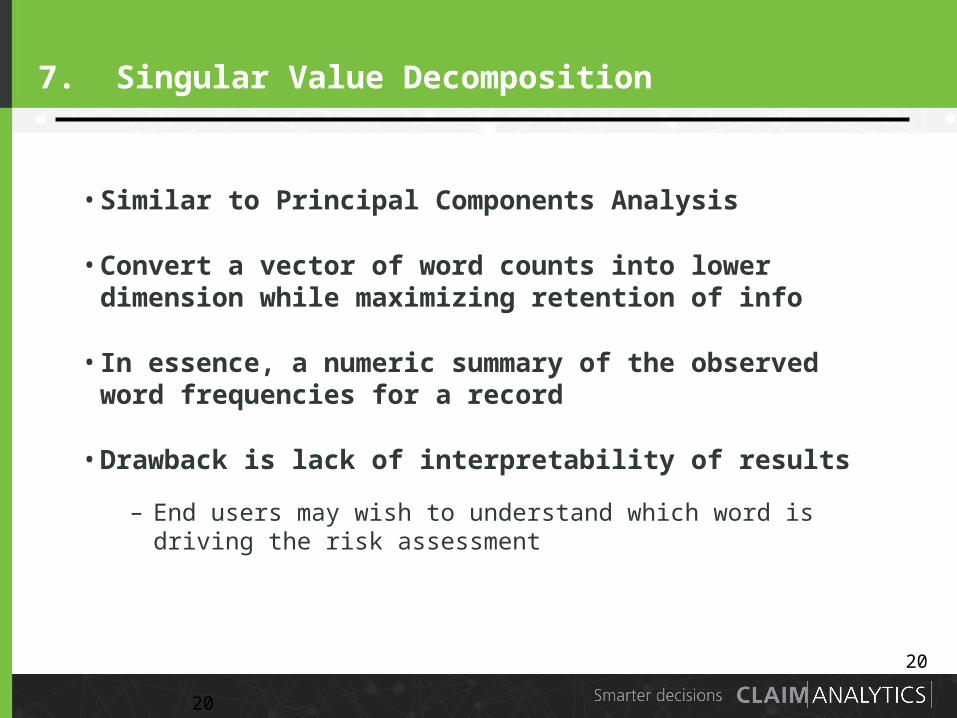
7. Singular Value Decomposition
• Similar to Principal Components Analysis
• Convert a vector of word counts into lower dimension while maximizing retention of info
• In essence, a numeric summary of the observed word frequencies for a record
• Drawback is lack of interpretability of results
– End users may wish to understand which word is driving the risk assessment
20

21
Word Frequencies by Record
Record Word1 Word2 Word50 Word100 Word200 Wordk
100001 1 0 0 0 1 0
100002 0 1 1 0 0 0
100003 0 0 0 1 0 1
100004 0 0 0 1 1 0
100005 1 0 0 0 0 0
100006 0 1 0 0 0 0
100007 1 0 1 0 0 0
100008 0 0 1 0 0 0
100009 0 0 0 0 1 1
21
22
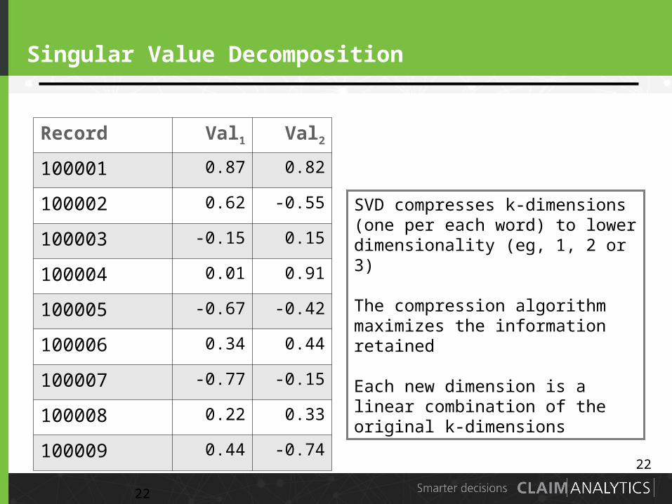
Singular Value Decomposition
Record Val1 Val2
100001 0.87 0.82
100002 0.62 -0.55
100003 -0.15 0.15
100004 0.01 0.91
100005 -0.67 -0.42
100006 0.34 0.44
100007 -0.77 -0.15
100008 0.22 0.33
100009 0.44 -0.74
22
SVD compresses k-dimensions (one per each word) to lower dimensionality (eg, 1, 2 or 3)
The compression algorithm maximizes the information retained
Each new dimension is a linear combination of the original k-dimensions
23
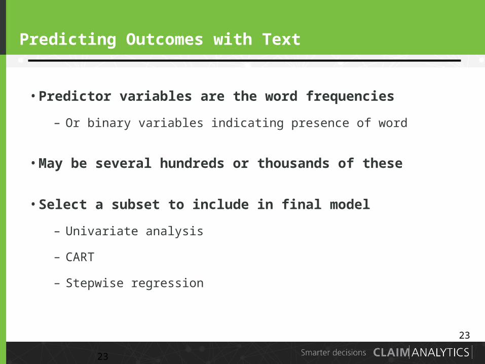
Predicting Outcomes with Text
• Predictor variables are the word frequencies
– Or binary variables indicating presence of word
• May be several hundreds or thousands of these
• Select a subset to include in final model
– Univariate analysis
– CART
– Stepwise regression
23

24
Stepwise Regression
• Backward stepwise regression:
– Build regression model with all variables
– Remove the one var that results in least loss of fit
– Continue until marginal decrease in fit > threshold
• Forward stepwise regression:
– Build regression model with one var with best fit
– Add the one variable that results in most lift
– Continue until marginal increase in lift < threshold
24

25
Case StudyResults

26
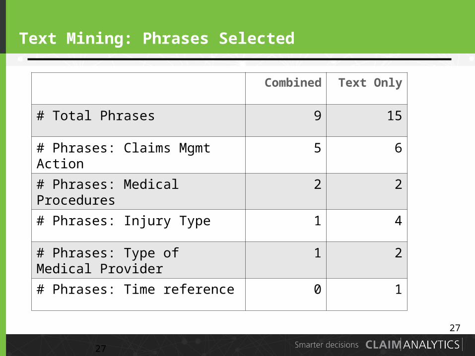
Text Mining: Phrases Selected
26
Combined Text Only
# Total Phrases 9 15
# Phrases: Claims Mgmt Action 5 6
# Phrases: Medical Procedures 2 2
# Phrases: Injury Type 1 4
# Phrases: Type of Medical Provider
1 2
# Phrases: Time reference 0 1
27
Text Mining: Phrases Selected
27
Combined Text Only
# Total Phrases 9 15
# Phrases: Claims Mgmt Action 5 6
# Phrases: Medical Procedures 2 2
# Phrases: Injury Type 1 4
# Phrases: Type of Medical Provider
1 2
# Phrases: Time reference 0 1
28
Model Evaluation
• Measuring goodness of fit should be performed on out-of-sample data
– Protects against overfit and ensures model is robust
– For this project, 10% of data was held back
• Measures for comparing goodness of fit include:
– Gains or lift charts
– Squared error
28

29
Cumulative Gains Chart - Baseline
29
% All Claims
────── Baseline────── Perfect
Area between the two curves is the model’s lift
30
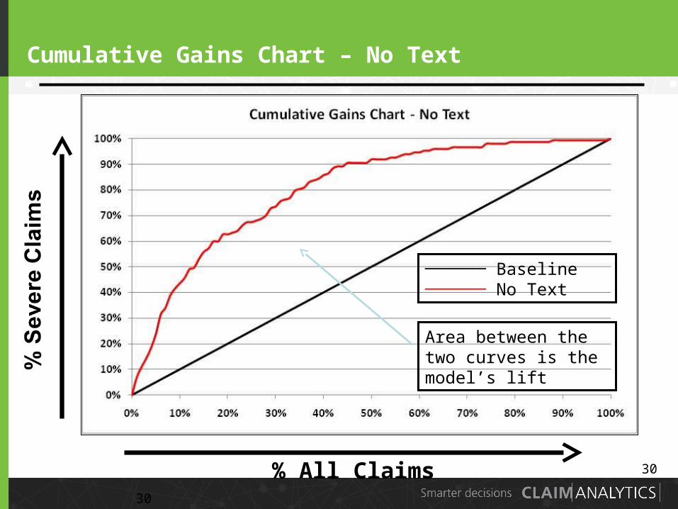
Cumulative Gains Chart – No Text
30
% All Claims
────── Baseline────── No Text
Area between the two curves is the model’s lift
31
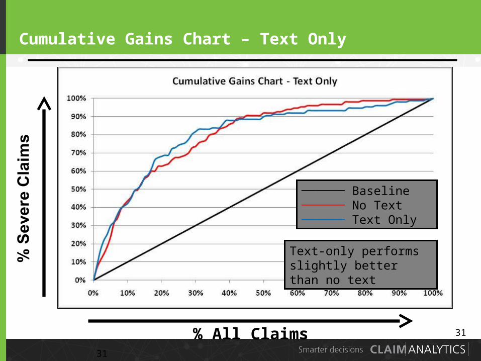
Cumulative Gains Chart – Text Only
31
% All Claims
────── Baseline────── No Text────── Text Only
Text-only performs slightly better than no text

32
Cumulative Gains Chart – Combined
32
% All Claims
────── Baseline────── No Text────── Text Only────── Combined
Combined text and non-text model performs best
33
Case Study Findings
•Text-only model slightly better than model without text
•Combined (text and non-text) model performs best
•Analyzing text can be simpler than summarizing medical bill transaction data
•Text mining is easy to interpret: certain words or phrases are correlated with higher or lower risk
•Text mining may provide extra lift for less experienced modelers
– Adding additional strong predictors may compensate for other modeling deficiencies
33

34
Questions
34
Top Related