


Languages
Pages
Legal

TESTING REGRESSION MONOTONICITY IN ECONOMETRIC MODELS
DENIS CHETVERIKOV
Abstract. Monotonicity is a key qualitative prediction of a wide array of economic models
derived via robust comparative statics. It is therefore important to design effective and practical
econometric methods for testing this prediction in empirical analysis. This paper develops a
general nonparametric framework for testing monotonicity of a regression function. Using this
framework, a broad class of new tests is introduced, which gives an empirical researcher a lot
of flexibility to incorporate ex ante information she might have. The paper also develops new
methods for simulating critical values, which are based on the combination of a bootstrap proce-
dure and new selection algorithms. These methods yield tests that have correct asymptotic size
and are asymptotically nonconservative. It is also shown how to obtain an adaptive rate optimal
test that has the best attainable rate of uniform consistency against models whose regression
function has Lipschitz-continuous first-order derivatives and that automatically adapts to the
unknown smoothness of the regression function. Simulations show that the power of the new
tests in many cases significantly exceeds that of some prior tests, e.g. that of Ghosal, Sen, and
Van der Vaart (2000). An application of the developed procedures to the dataset of Ellison and
Ellison (2011) shows that there is some evidence of strategic entry deterrence in pharmaceutical
industry where incumbents may use strategic investment to prevent generic entries when their
patents expire.
1. Introduction
The concept of monotonicity plays an important role in economics. For example, monotone
comparative statics has been a popular research topic in economic theory for many years; see,
in particular, the seminal work on this topic by Milgrom and Shannon (1994) and Athey (2002).
Matzkin (1994) mentions monotonicity as one of the most important implications of economic
theory that can be used in econometric analysis. Given importance of monotonicity in economic
theory, the natural question is whether we observe monotonicity in the data. Although there
do exist some methods for testing monotonicity in statistics, there is no general theory that
would suffice for empirical analysis in economics. For example, I am not aware of any test
of monotonicity that would allow for multiple covariates. In addition, there are currently no
Date: First version: March 2012. This version: December 3, 2013. Email: [email protected]. I thank
Victor Chernozhukov for encouragement and guidance. I am also grateful to Anna Mikusheva, Isaiah Andrews,
Andres Aradillas-Lopez, Moshe Buchinsky, Glenn Ellison, Jin Hahn, Bo Honore, Rosa Matzkin, Jose Montiel,
Ulrich Muller, Whitney Newey, and Jack Porter for valuable comments. The first version of the paper was
presented at the Econometrics lunch at MIT in April, 2012.
1

2 DENIS CHETVERIKOV
published results on testing monotonicity that would allow for endogeneity of covariates. Such
a theory is provided in this paper. In particular, this paper provides a general nonparametric
framework for testing monotonicity of a regression function. Tests of monotonicity developed in
this paper can be used to evaluate assumptions and implications of economic theory concerning
monotonicity. In addition, as was recently noticed by Ellison and Ellison (2011), these tests can
also be used to provide evidence of existence of certain phenomena related to strategic behavior of
economic agents that are difficult to detect otherwise. Several motivating examples are presented
in the next section.
I start with the model
Y = f(X) + ε (1)
where Y is a scalar dependent random variable, X a scalar independent random variable, f(·)an unknown function, and ε an unobserved scalar random variable satisfying E[ε|X] = 0 almost
surely. Later in the paper, I extend the analysis to cover models with multivariate and endogenous
X’s. I am interested in testing the null hypothesis, H0, that f(·) is nondecreasing against the
alternative, Ha, that there are x1 and x2 such that x1 < x2 but f(x1) > f(x2). The decision is
to be made based on the i.i.d. sample of size n, {Xi, Yi}16i6n from the distribution of (X,Y ). I
assume that f(·) is smooth but do not impose any parametric structure on it. I derive a theory
that yields tests with the correct asymptotic size. I also show how to obtain consistent tests and
how to obtain a test with the optimal rate of uniform consistency against classes of functions
with Lipschitz-continuous first order derivatives. Moreover, the rate optimal test constructed in
this paper is adaptive in the sense that it automatically adapts to the unknown smoothness of
f(·).
This paper makes several contributions. First, I introduce a general framework for testing
monotonicity. This framework allows me to develop a broad class of new tests, which also includes
some existing tests as special cases. This gives a researcher a lot of flexibility to incorporate ex
ante information she might have. Second, I develop new methods to simulate the critical values
for these tests that in many cases yield higher power than that of existing methods. Third, I
consider the problem of testing monotonicity in models with multiple covariates for the first time
in the literature. As will be explained in the paper, these models are more difficult to analyze
and require a different treatment in comparison with the case of univariate X. Finally, I consider
models with endogenous X that are identified via instrumental variables, and I consider models
with sample selection.
Providing a general framework for testing monotonicity is a difficult problem. The problem
arises because different test statistics studied in this paper have different limit distributions
and require different normalizations. Some of the test statistics have N(0, 1) limit distribution,
and some others have an extreme value limit distribution. Importantly, there are also many
TESTING REGRESSION MONOTONICITY 3
test statistics that are “in between”, so that their distributions are far both from N(0, 1) and
from extreme value distributions, and so their asymptotic approximations are difficult to obtain.
Moreover, and equally important, the limit distribution of the statistic that leads to the rate
optimal and adaptive test is unknown. The main difficulty here is that the processes underlying
the test statistic do not have an asymptotic equicontinuity property, and so classical functional
central limit theorems, as presented for example in Van der Vaart and Wellner (1996) and Dudley
(1999), do not apply. This paper addresses these issues and provide bootstrap critical values
that are valid uniformly over a large class of different test statistics and different data generating
processes. Two previous papers, Hall and Heckman (2000) and Ghosal, Sen, and van der Vaart
(2000), used specific techniques to prove validity of their tests of monotonicity but it is difficult to
generalize their techniques to make them applicable for other tests of monotonicity. In contrast,
in this paper, I introduce a general approach that can be used to prove validity of many different
tests of monotonicity. Other shape restrictions, such as concavity and super-modularity, can be
tested by procedures similar to those developed in this paper.
Another problem is that test statistics studied in this paper have some asymptotic distribution
when f(·) is constant but diverge if f(·) is strictly increasing. This discontinuity implies that
for some sequences of models f(·) = fn(·), the limit distribution depends on the local slope
function, which is an unknown infinite-dimensional nuisance parameter that can not be estimated
consistently from the data. A common approach in the literature to solve this problem is to
calibrate the critical value using the case when the type I error is maximized (the least favorable
model), i.e. the model with constant f(·).1 In contrast, I develop two selection procedures that
estimate the set where f(·) is not strictly increasing, and then adjust the critical value to account
for this set. The estimation is conducted so that no violation of the asymptotic size occurs. The
critical values obtained using these selection procedures yield important power improvements
in comparison with other tests if f(·) is strictly increasing over some subsets of the support of
X. The first selection procedure, which is based on the one-step approach, is related to those
developed in Chernozhukov, Lee, and Rosen (2013), Andrews and Shi (2010), and Chetverikov
(2012), all of which deal with the problem of testing conditional moment inequalities. The second
selection procedure is novel and is based on the step-down approach. It is somewhat related to
methods developed in Romano and Wolf (2005a) and Romano and Shaikh (2010) but the details
are rather different.
Further, an important issue that applies to nonparametric testing in general is how to choose
a smoothing parameter for the test. In theory, the optimal smoothing parameter can be derived
for many smoothness classes of functions f(·). In practice, however, the smoothness class that
f(·) belongs to is usually unknown. I deal with this problem by employing the adaptive testing
1The exception is Wang and Meyer (2011) who use the model with an isotonic estimate of f(·) to simulate the
critical value. They do not prove whether their test maintains the required size, however.
4 DENIS CHETVERIKOV
approach. This allows me to obtain tests with good power properties when the information
about smoothness of the function f(·) possessed by the researcher is absent or limited. More
precisely, I construct a test statistic using many different weighting functions that correspond to
many different values of the smoothing parameter so that the distribution of the test statistic is
mainly determined by the optimal weighting function. I provide a basic set of weighting functions
that yields a rate optimal and adaptive test and show how the researcher can change this set in
order to incorporate ex ante information. Importantly, the approach taken in this paper does
not require “under-smoothing”. This feature of my approach is important because, to the best
of my knowledge, all procedures in the literature to achieve “under-smoothing” are ad hoc and
do not have a sound theoretical justification.
The literature on testing monotonicity of a nonparametric regression function is quite large.
The tests of Gijbels et. al. (2000) and Ghosal, Sen, and van der Vaart (2000) (from now on, GHJK
and GSV, respectively) are based on the signs of (Yi+k−Yi)(Xi+k−Xi). Hall and Heckman (2000)
(from now on, HH) developed a test based on the slopes of local linear estimates of f(·). The
list of other papers includes Schlee (1982), Bowman, Jones, and Gijbels (1998), Dumbgen and
Spokoiny (2001), Durot (2003), Beraud, Huet, and Laurent (2005), and Wang and Meyer (2011).
In a contemporaneous work, Lee, Song, and Whang (2011b) derive another approach to testing
monotonicity based on Lp-functionals. The results in this paper complement the results of that
paper. An advantage of their method is that the asymptotic distribution of their test statistic
in the least favorable model under H0 turns out to be N(0, 1), so that obtaining a critical value
for their test is computationally very simple. A disadvantage of their method, however, is that
their test is not adaptive. Results in this paper are also different from those in Romano and Wolf
(2011) who also consider the problem of testing monotonicity. In particular, they assume that
X is non-stochastic and discrete, which makes their problem semi-parametric and substantially
simplifies proving validity of critical values, and they test the null hypothesis that f(·) is not
weakly increasing against the alternative that it is weakly increasing. Lee, Linton, and Whang
(2009) and Delgado and Escanciano (2010) derived tests of stochastic monotonicity, which is a
related but different problem. Specifically, stochastic monotonicity means that the conditional
cdf of Y given X, FY |X(y, x), is (weakly) decreasing in x for any fixed y.
As an empirical application of the results developed in this paper, I consider the problem of
detecting strategic entry deterrence in the pharmaceutical industry. In that industry, incumbents
whose drug patents are about to expire can change their investment behavior in order to prevent
generic entries after the expiration of the patent. Although there are many theoretically com-
pelling arguments as to how and why incumbents should change their investment behavior (see,
for example, Tirole (1988)), the empirical evidence is rather limited. Ellison and Ellison (2011)
showed that, under certain conditions, the dependence of investment on market size should be
monotone if no strategic entry deterrence is present. In addition, they noted that the entry
TESTING REGRESSION MONOTONICITY 5
deterrence motive should be important in intermediate-sized markets and less important in small
and large markets. Therefore, strategic entry deterrence might result in the non-monotonicity of
the relation between market size and investment. Hence, rejecting the null hypothesis of mono-
tonicity provides the evidence in favor of the existence of strategic entry deterrence. I apply
the tests developed in this paper to Ellison and Ellison’s dataset and show that there is some
evidence of non-monotonicity in the data. The evidence is rather weak, though.
The rest of the paper is organized as follows. Section 2 provides motivating examples. Section
3 describes the general test statistic and gives several methods to simulate the critical value.
Section 4 contains the main results under high-level conditions when there are no additional
covariates. Since in most practically relevant cases, the model also contains some additional
covariates, Section 5 studies the cases of fully nonparametric and partially linear models with
multiple covariates. Section 6 extends the analysis to cover the case where X is endogenous and
identification is achieved via instrumental variables. Section 7 briefly explains how to test mono-
tonicity in sample selection models. Section 8 presents a small Monte Carlo simulation study.
Section 9 describes the empirical application. Section 10 concludes. All proofs are contained
in the Appendix. In addition, Appendix A contains implementation details, and Appendix B is
devoted to the verification of high-level conditions under primitive assumptions.
Notation. Throughout this paper, let {εi} denote a sequence of independent N(0, 1) random
variables that are independent of the data. The sequence {εi} will be used in bootstrapping
critical values. The notation i = 1, n is a shorthand for i ∈ {1, ..., n}. For any set S, I denote the
number of elements in this set by |S|.
2. Motivating Examples
Many testable implications of economic theory are concerned with comparative statics analy-
sis. These implications most often take the form of qualitative statements like “Increasing factor
X will positively (negatively) affect response variable Y ”. The common approach to test such
implications on the data is to look at the corresponding coefficient in the linear (or other para-
metric) regression. Relying on these strong parametric assumptions, however, can lead to highly
misleading results. For example, the test based on the linear regression will not be consistent and
the test based on the quadratic regression may severely over-reject if the model is misspecified.
In contrast, this paper provides a class of tests that are valid without these strong parametric
assumptions. The purpose of this section is to give three examples from the literature where
tests developed in this paper can be applied.
1. Detecting strategic effects. Certain strategic effects, the existence of which is difficult
to prove otherwise, can be detected by testing for monotonicity. An example on strategic entry
deterrence in the pharmaceutical industry is described in the Introduction and is analyzed in
6 DENIS CHETVERIKOV
Section 9. Below I provide another example concerned with the problem of debt pricing. This
example is based on Morris and Shin (2003). Consider a model where investors hold a collat-
eralized debt. The debt will yield a fixed payment, say 1, in the future if it is rolled over and
an underlying project is successful. Otherwise the debt will yield nothing (0). Alternatively, all
investors have an option of not rolling over and getting the value of the collateral, κ ∈ (0, 1),
immediately. The probability that the project turns out to be successful depends on the funda-
mentals, θ, and on how many investors roll over. Specifically, assume that the project is successful
if θ exceeds the proportion of investors who roll over. Under global game reasoning, if private
information possessed by investors is sufficiently accurate, the project will succeed if and only if
θ > κ; see Morris and Shin (2003) for details. Then ex ante value of the debt is given by
V (κ) = κ · P(θ < κ) + 1 · P(θ > κ),
and the derivative of the ex ante debt value with respect to the collateral value is
dV (κ)
dκ= P(θ < κ)− (1− κ)
dP(θ < κ)
dκ
The first and second terms on the right hand side of this equation represent direct and strategic
effects, respectively. The strategic effect represents coordination failure among investors. It
arises because high value of the collateral leads investors to believe that many other investors
will not roll over, and the project will not be successful even though the project is profitable
(κ < 1). Morris and Shin (2004) argue that this effect is important for understanding anomalies
in empirical implementation of the standard debt pricing theory of Merton (1974). A natural
question is how to prove existence of this effect in the data. Note that in the absence of strategic
effect, the relation between value of the debt and value of the collateral will be monotonically
increasing. If strategic effect is sufficiently strong, however, it can cause non-monotonicity in this
relation. Therefore, one can detect the existence of the strategic effect and coordination failure
by testing whether conditional mean of the price of the debt given the value of the collateral
is a monotonically increasing function. Rejecting the null hypothesis of monotonicity provides
evidence in favor of the existence of the strategic effect and coordination failure.
2. Testing assumptions of treatment effect models. Monotonicity is often assumed in
the econometrics literature on estimating treatment effects. A widely used econometric model
in this literature is as follows. Suppose that we observe a sample of individuals, i = 1, n. Each
individual has a random response function yi(t) that gives her response for each level of treatment
t ∈ T . Let zi and yi = yi(zi) denote the realized level of the treatment and the realized response,
respectively (both are observable). The problem is how to derive inference on E[yi(t)]. To
address this problem, Manski and Pepper (2000) introduced assumptions of monotone treatment
response, which imposes that yi(t2) > yi(t1) whenever t2 > t1, and monotone treatment selection,
which imposes that E[yi(t)|zi = v] is increasing in v for all t ∈ T . The combination of these
TESTING REGRESSION MONOTONICITY 7
assumptions yields a testable prediction. Indeed, for all v2 > v1,
E[yi|zi = v2] = E[yi(v2)|zi = v2]
> E[yi(v1)|zi = v2] > E[yi(v1)|zi = v1] = E[yi|zi = v1].
Since both zi and yi are observed, this prediction can be tested by the procedures developed in
this paper. Note that the tests of stochastic monotonicity as described in the Introduction do
not apply here since the testable prediction is monotonicity of the conditional mean function.
3. Testing the theory of the firm. A classical paper Holmstrom and Milgrom (1994)
on the theory of the firm is built around the observation that in multi-task problems different
incentive instruments are expected to be complementary to each other. Indeed, increasing an
incentive for one task may lead the agent to spend too much time on that task ignoring other
responsibilities. This can be avoided if incentives on different tasks are balanced with each other.
To derive testable implications of the theory, Holmstrom and Milgrom study a model of industrial
selling introduced in Anderson and Schmittlein (1984) where a firm chooses between an in-house
agent and an independent representative who divide their time into four tasks: (i) direct sales,
(ii) investing in future sales to customers, (iii) non-sale activities, such as helping other agents,
and (iv) selling the products of other manufacturers. Proposition 4 in their paper states that
under certain conditions, the conditional probability of having an in-house agent is a (weakly)
increasing function of the marginal cost of evaluating performance and is a (weakly) increasing
function of the importance of non-selling activities. These are hypotheses that can be directly
tested on the data by procedures developed in this paper. This would be an important extension
of linear regression analysis performed, for example, in Anderson and Schmittlein (1984) and
Poppo and Zenger (1998). Again, note that the tests of stochastic monotonicity as described in
the Introduction do not apply here.
3. The Test
3.1. The General Test Statistic. Recall that I consider a model given in equation (1), and the
test should be based on the i.i.d. sample {Xi, Yi}16i6n of n observations from the distribution of
(X,Y ) where X and Y are independent and dependent random variables, respectively. In this
section and in Section 4, I assume that X is a scalar and there are no additional covariates Z.
The case where additional covariates Z are present is considered in Section 5.
Let Q(·, ·) : R × R → R be a weighting function satisfying Q(x1, x2) = Q(x2, x1) and
Q(x1, x2) > 0 for all x1, x2 ∈ R, and let
b = b({Xi, Yi}) = (1/2)∑
16i,j6n
(Yi − Yj)sign(Xj −Xi)Q(Xi, Xj)
8 DENIS CHETVERIKOV
be a test function. Since Q(Xi, Xj) > 0 and E[Yi|Xi] = f(Xi), it is easy to see that under H0,
that is, when the function f(·) is non-decreasing, E[b] 6 0. On the other hand, if H0 is violated
and there exist x1 and x2 on the support of X such that x1 < x2 but f(x1) > f(x2), then there
exists a function Q(·, ·) such that E[b] > 0 if f(·) is smooth. Therefore, b can be used to form a
test statistic if I can find an appropriate function Q(·, ·). For this purpose, I will use the adaptive
testing approach developed in statistics literature. Even though this approach has attractive
features, it is almost never used in econometrics. A notable exception is Horowitz and Spokoiny
(2001), who used it for specification testing.
The idea behind the adaptive testing approach is to choose Q(·, ·) from a large set of potentially
useful weighting functions that maximizes the studentized version of b. Formally, let Sn be some
general set that depends on n and is (implicitly) allowed to depend on {Xi}, and for s ∈ Sn, let
Q(·, ·, s) : R×R→ R be some function satisfying Q(x1, x2, s) = Q(x2, x1, s) and Q(x1, x2, s) > 0
for all x1, x2 ∈ R. The functions Q(·, ·, s) are also (implicitly) allowed to depend on {Xi}. In
addition, let
b(s) = b({Xi, Yi}, s) = (1/2)∑
16i,j6n
(Yi − Yj)sign(Xj −Xi)Q(Xi, Xj , s) (2)
be a test function. Conditional on {Xi}, the variance of b(s) is given by
V (s) = V ({Xi}, {σi}, s) =∑
16i6n
σ2i
∑16j6n
sign(Xj −Xi)Q(Xi, Xj , s)
2
(3)
where σi = (E[ε2i |Xi])
1/2 and εi = Yi − f(Xi). In general, σi’s are unknown, and have to
be estimated from the data. Let σi denote some (not necessarily consistent) estimator of σi.
Available estimators are discussed later in this section. Then the estimated conditional variance
of b(s) is
V (s) = V ({Xi}, {σi}, s) =∑
16i6n
σ2i
∑16j6n
sign(Xj −Xi)Q(Xi, Xj , s)
2
. (4)
The general form of the test statistic that I consider in this paper is
T = T ({Xi, Yi}, {σi},Sn) = maxs∈Sn
b({Xi, Yi}, s)√V ({Xi}, {σi}, s)
. (5)
Large values of T indicate that the null hypothesis is violated. Later in this section, I will provide
methods for estimating quantiles of T underH0 and for choosing a critical value for the test based
on the statistic T .
The set Sn determines adaptivity properties of the test, that is the ability of the test to
detect many different deviations from H0. Indeed, each weighting function Q(·, ·, s) is useful for
detecting some deviation, and so the larger is the set of weighting functions Sn, the larger is
TESTING REGRESSION MONOTONICITY 9
the number of different deviations that can be detected, and the higher is adaptivity of the test.
In this paper, I allow for exponentially large (in the sample size n) sets Sn. This implies that
the researcher can choose a huge set of weighting functions, which allows her to detect large
set of different deviations from H0. The downside of the adaptivity, however, is that expanding
the set Sn increases the critical value, and thus decreases the power of the test against those
alternatives that can be detected by weighting functions already included in Sn. Fortunately, in
many cases the loss of power is relatively small. In particular, it follows from Lemma D.1 and
Borell’s inequality (see Proposition A.2.1 in Van der Vaart and Wellner (1996)) that the critical
values for test developed below are bounded from above by a slowly growing C(log p)1/2 for some
C > 0 where p = |Sn|, the number of elements in the set Sn.
3.2. Typical Weighting Functions. Let me now describe typical weighting functions. Con-
sider some compactly supported kernel function K : R → R satisfying K(x) > 0 for all x ∈ R.
For convenience, I will assume that the support of K is [−1, 1]. In addition, let s = (x, h) where
x is a location point and h is a bandwidth value (smoothing parameter). Finally, define
Q(x1, x2, (x, h)) = |x1 − x2|kK(x1 − xh
)K
(x2 − xh
)(6)
for some k > 0. I refer to this Q as a kernel weighting function.2
Assume that a test is based on kernel weighting functions and Sn consists of pairs s = (x, h)
with many different values of x and h. To explain why this test has good adaptivity properties,
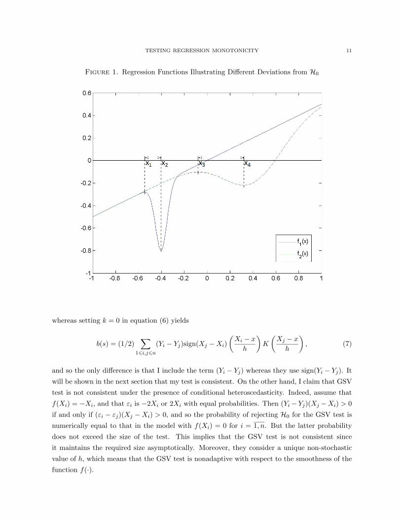
consider figure 1 that plots two regression functions. Both f1(·) and f2(·) violate H0 but locations
where H0 is violated are different. In particular, f1(·) violates H0 on the interval [x1, x2] and
f2(·) violates H0 on the interval [x3, x4]. In addition, f1(·) is relatively less smooth than f2(·),and [x1, x2] is shorter than [x3, x4]. To have good power against f1(·), Sn should contain a pair
(x, h) such that [x− h, x+ h] ⊂ [x1, x2]. Indeed, if [x− h, x+ h] is not contained in [x1, x2], then
positive and negative values of the summand of b will cancel out yielding a low value of b. In
particular, it should be the case that x ∈ [x1, x2]. Similarly, to have good power against f2(·),Sn should contain a pair (x, h) such that x ∈ [x3, x4]. Therefore, using many different values of
x yields a test that adapts to the location of the deviation from H0. This is spatial adaptivity.
Further, note that larger values of h yield higher signal-to-noise ratio. So, given that [x3, x4] is
longer than [x1, x2], the optimal pair (x, h) to test against f2(·) has larger value of h than that to
test against f1(·). Therefore, using many different values of h results in adaptivity with respect
to smoothness of the function, which, in turn, determines how fast its first derivative is varying
and how long the interval of non-monotonicity is.
2It is possible to extend the definition of kernel weighting functions given in (6). Specifically, the term |x1−x2|k
in the definition can be replaced by general function K(x1, x2) satisfying K(x1, x2) > 0 for all x1 and x2. I thank
Joris Pinkse for this observation.
10 DENIS CHETVERIKOV
If no ex ante information is available, I recommend using kernel weighting functions with
Sn = {(x, h) : x ∈ {X1, ..., Xn}, h ∈ Hn} where Hn = {h = hmaxul : h > hmin, l = 0, 1, 2, ...} and
hmax = max16i,j6n |Xi −Xj |/2. I also recommend setting u = 0.5, hmin = 0.4hmax(log n/n)1/3,
and k = 0 or 1. I refer to this Sn as a basic set of weighting functions. This choice of parameters is
consistent with the theory presented in this paper and has worked well in simulations. The basic
set of weighting functions yields a rate optimal and adaptive test. The value of hmin is selected
so that the test function b(s) for any given s uses no less than approximately 15 observations
when n = 100 and X is distributed uniformly on some interval.
If some ex ante information is available, the general framework considered here gives the
researcher a lot of flexibility to incorporate this information. In particular, if the researcher
expects that the function f(·) is rather smooth, then the researcher can restrict the set Sn by
considering only pairs (x, h) with large values of h since in this case deviations from H0, if
present, are more likely to happen on long intervals. Moreover, if the smoothness of the function
f(·) is known, one can find an optimal value of the smoothing parameter h = hn corresponding
to this level of smoothness, and then consider kernel weighting functions with this particular
choice of the bandwidth value, that is Sn = {(x, h) : x ∈ {X1, ..., Xn}, h = h}. Further, if non-
monotonicity is expected at one particular point x, one can consider kernel weighting functions
with Sn = {(x, h) : x = x, h = h} or Sn = {(x, h) : x = x, h ∈ Hn} depending on whether
smoothness of f(·) is known or not. More broadly, if non-monotonicity is expected on some
interval X , one can use kernel weighting functions with Sn = {(x, h) : x ∈ {X1, ..., Xn}∩X , h ∈ h}or Sn = {(x, h) : x ∈ {X1, ..., Xn} ∩ X , h ∈ Hn} again depending on whether smoothness of f(·)is known or not. Note that all these modifications will increase the power of the test because
smaller sets Sn yield lower critical values.
Another interesting choice of the weighting functions is
Q(x1, x2, s) =∑
16r6m
|x1 − x2|kK(x1 − xr
h
)K
(x2 − xr
h
)where s = (x1, ..., xm, h). These weighting functions are useful if the researcher expects multiple
deviations from H0.
3.3. Comparison with Other Known Tests. I will now show that the general framework de-
scribed above includes the Hall and Heckman’s (HH) test statistic and a slightly modified version
of the Ghosal, Sen, and van der Vaart’s (GSV) test statistic as special cases that correspond to
different values of k in the definition of kernel weighting functions.
GSV use the following test function:
b(s) = (1/2)∑
16i,j6n
sign(Yi − Yj)sign(Xj −Xi)K
(Xi − xh
)K
(Xj − xh
),
TESTING REGRESSION MONOTONICITY 11
Figure 1. Regression Functions Illustrating Different Deviations from H0
whereas setting k = 0 in equation (6) yields
b(s) = (1/2)∑
16i,j6n
(Yi − Yj)sign(Xj −Xi)
(Xi − xh
)K
(Xj − xh
), (7)
and so the only difference is that I include the term (Yi − Yj) whereas they use sign(Yi − Yj). It
will be shown in the next section that my test is consistent. On the other hand, I claim that GSV
test is not consistent under the presence of conditional heteroscedasticity. Indeed, assume that
f(Xi) = −Xi, and that εi is −2Xi or 2Xi with equal probabilities. Then (Yi− Yj)(Xj −Xi) > 0
if and only if (εi − εj)(Xj −Xi) > 0, and so the probability of rejecting H0 for the GSV test is
numerically equal to that in the model with f(Xi) = 0 for i = 1, n. But the latter probability
does not exceed the size of the test. This implies that the GSV test is not consistent since
it maintains the required size asymptotically. Moreover, they consider a unique non-stochastic
value of h, which means that the GSV test is nonadaptive with respect to the smoothness of the
function f(·).
12 DENIS CHETVERIKOV
Let me now consider the HH test. The idea of this test is to make use of local linear estimates
of the slope of the function f(·). Using well-known formulas for the OLS regression, it is easy
to show that the slope estimate of the function f(·) given the data {Xi, Yi}s2i=s1+1 with s1 < s2
where {Xi}ni=1 is an increasing sequence is given by
b(s) =
∑s1<i6s2 Yi
∑s1<j6s2(Xi −Xj)
(s2 − s1)∑
s1<i6s2 X2i − (
∑s1<i6s2 Xi)2
, (8)
where s = (s1, s2). Note that the denominator of (8) depends only on Xi’s, and so it disappears
after studentization. In addition, simple rearrangements show that the numerator in (8) is up to
the sign is equal to
(1/2)∑
16i,j6n
(Yi − Yj)(Xj −Xi)1{x− h 6 Xi 6 x+ h}1{x− h 6 Xj 6 x+ h} (9)
for some x and h. On the other hand, setting k = 1 in equation (6) yields
b(s) = (1/2)∑
16i,j6n
(Yi − Yj)(Xj −Xi)K
(Xi − xh
)K
(Xj − xh
). (10)
Noting that expression in (9) is proportional to that on the right hand side in (10) with K(·) =
1{[−1,+1]}(·) implies that the HH test statistic is a special case of those studied in this paper.
3.4. Estimating σi. In practice, σi’s are usually unknown, and, hence, have to be estimated
from the data. Let σi denote some estimator of σi. I provide results for two types of estimators.
The first type of estimators is easier to implement but the second worked better in simulations.
First, σi can be estimated by the residual εi. More precisely, let f(·) be some uniformly consis-
tent estimator of f(·) with a polynomial rate of consistency in probability, i.e. f(Xi)− f(Xi) =
op(n−κ1) uniformly over i = 1, n for some κ1 > 0, and let σi = εi where εi = Yi−f(Xi). Note that
σi can be negative. Clearly, σi is not a consistent estimator of σi. Nevertheless, as I will show
in Section 4 that this estimator leads to valid inference. Intuitively, it works because the test
statistic contains the weighted average sum of σ2i over i = 1, n, and the estimation error averages
out. To obtain a uniformly consistent estimator f(·) of f(·), one can use a series method (see
Newey (1997), theorem 1) or local polynomial method (see Tsybakov (2009), theorem 1.8). If one
prefers kernel methods, it is important to use generalized kernels in order to deal with bound-
ary effects when higher order kernels are used; see, for example, Muller (1991). Alternatively,
one can choose Sn so that boundary points are excluded from the test statistic. In addition,
if the researcher decides to impose some parametric structure on the set of potentially possi-
ble heteroscedasticity functions, then parametric methods like OLS will typically give uniform
consistency with κ1 arbitrarily close to 1/2.
The second way of estimating σi is to use a parametric or nonparametric estimator σi satisfying
σi − σi = op(n−κ2) uniformly over i = 1, n for some κ2 > 0. Many estimators of σi satisfy this
TESTING REGRESSION MONOTONICITY 13
condition. Assume that the observations {Xi, Yi}ni=1 are arranged so that Xi 6 Xj whenever
i 6 j. Then the estimator of Rice (1984), given by
σ =
(1
2n
n−1∑i=1
(Yi+1 − Yi)2
)1/2
, (11)
is√n-consistent if σi = σ for all i = 1, n and f(·) is piecewise Lipschitz-continuous.
The Rice estimator can be easily modified to allow for conditional heteroscedasticity. Choose
a bandwidth value bn > 0. For i = 1, n, let J(i) = {j = 1, n : |Xj −Xi| 6 bn}. Let |J(i)| denote
the number of elements in J(i). Then σi can be estimated by
σi =
1
2|J(i)|∑
j∈J(i):j+1∈J(i)
(Yj+1 − Yj)2
1/2
. (12)
I refer to (12) as a local version of Rice’s estimator. An advantage of this estimator is that it
is adaptive with respect to the smoothness of the function f(·). Proposition B.1 in Appendix B
provides conditions that are sufficient for uniform consistency of this estimator with a polynomial
rate. The key condition there is that |σj+1 − σj | 6 C|Xj+1 − Xj | for some C > 0 and all
j = 1, n− 1. The intuition for consistency is as follows. Note that Xj+1 is close to Xj . So, if the
function f is continuous, then
Yj+1 − Yj = f(Xj+1)− f(Xj) + εj+1 − εj ≈ εj+1 − εj ,
so that
E[(Yj+1 − Yj)2|{Xi}] ≈ σ2j+1 + σ2
j
since εj+1 is independent of εj . Further, if bn is sufficiently small, then σ2j+1 + σ2
j ≈ 2σ2i since
|Xj+1 − Xi| 6 bn and |Xj − Xi| 6 bn, and so σ2i is close to σ2
i . Other available estimators are
presented, for example, in Muller and Stadtmuller (1987), Fan and Yao (1998), Horowitz and
Spokoiny (2001), Hardle and Tsybakov (2007), and Cai and Wang (2008).
3.5. Simulating the Critical Value. In this subsection, I provide three different methods for
estimating quantiles of the null distribution of the test statistic T . These are plug-in, one-step,
and step-down methods. All of these methods are based on the procedure known as the Wild
bootstrap. The Wild bootstrap was introduced in Wu (1986) and used, among many others, by
Liu (1988), Mammen (1993), Hardle and Mammen (1993), Horowitz and Spokoiny (2001), and
Chetverikov (2012). See also Chernozhukov, Chetverikov, and Kato (2012). The three methods
are arranged in terms of increasing power and computational complexity. The validity of all
three methods is established in theorem 4.1. Recall that {εi} denotes a sequence of independent
N(0, 1) random variables that are independent of the data.
14 DENIS CHETVERIKOV
Plug-in Approach. Suppose that we want to obtain a test of level α. The plug-in approach is
based on two observations. First, under H0,
b(s) = (1/2)∑
16i,j6n
(f(Xi)− f(Xj) + εi − εj)sign(Xj −Xi)Q(Xi, Xj , s) (13)
6 (1/2)∑
16i,j6n
(εi − εj)sign(Xj −Xi)Q(Xi, Xj , s) (14)
since Q(Xi, Xj , s) > 0 and f(Xi) > f(Xj) whenever Xi > Xj under H0, and so the (1 − α)
quantile of T is bounded from above by the (1 − α) quantile of T in the model with f(x) = 0
for all x ∈ R, which is the least favorable model under H0. Second, it will be shown that the
distribution of T asymptotically depends on the distribution of noise {εi} only through {σ2i }.
These two observations suggest that the critical value for the test can be obtained by simulating
the conditional (1 − α) quantile of T ? = T ({Xi, Yi?}, {σi},Sn) given {Xi}, {σi}, and Sn where
Y ?i = σiεi for i = 1, n. This is called the plug-in critical value cPI1−α. See Section A of the
Appendix for detailed step-by-step instructions.
One-Step Approach. The test with the plug-in critical value is computationally rather simple.
It has, however, poor power properties. Indeed, the distribution of T in general depends on f(·)but the plug-in approach is based on the least favorable regression function f(x) = 0 for all x ∈ R,
and so it is too conservative when f(·) is strictly increasing. More formally, suppose for example
that kernel weighting functions are used, and that f(·) is strictly increasing in h-neighborhood
of x1 but is constant in h-neighborhood of x2. Let s1 = s(x1, h) and s2 = s(x2, h). Then
b(s1)/(V (s1))1/2 is no greater than b(s2)/(V (s2))1/2 with probability approaching one. On the
other hand, b(s1)/(V (s1))1/2 is greater than b(s2)/(V (s2))1/2 with nontrivial probability in the
model with f(x) = 0 for all x ∈ R, which is used to obtain cPI1−α. Therefore, cPI1−α overestimates
the corresponding quantile of T . The natural idea to overcome the conservativeness of the plug-
in approach is to simulate a critical value using not all elements of Sn but only those that are
relevant for the given sample. In this paper, I develop two selection procedures that are used to
decide what elements of Sn should be used in the simulation. The main difficulty here is to make
sure that the selection procedures do not distort the size of the test. The simpler of these two
procedures is the one-step approach.
Let {γn} be a sequence of positive numbers converging to zero, and let cPI1−γn be the (1− γn)
plug-in critical value. In addition, denote
SOSn = SOSn ({Xi, Yi}, {σi},Sn) = {s ∈ Sn : b(s)/(V (s))1/2 > −2cPI1−γn}.
Then the one-step critical value cOS1−α is the conditional (1−α) quantile of the simulated statistic
T ? = T ({Xi, Yi?}, {σi},SOSn ) given {Xi}, {σi}, and SOSn where Y ?
i = σiεi for i = 1, n.3 Intuitively,
3If SOSn turns out to be empty, assume that SOSn consists of one randomly chosen element of Sn.
TESTING REGRESSION MONOTONICITY 15
the one-step critical value works because the weighting functions corresponding to elements of
the set Sn\SOSn have an asymptotically negligible influence on the distribution of T under H0.
Indeed, it will be shown that the probability that at least one element s of Sn such that
(1/2)∑
16i,j6n
(f(Xi)− f(Xj))sign(Xj −Xi)Q(Xi, Xj , s)/(V (s))1/2 > −cPI1−γn (15)
belongs to the set Sn\SOSn is at most γn+o(1). On the other hand, the probability that at least one
element s of Sn such that inequality (15) does not hold for this element gives b(s)/(V (s))1/2 > 0
is again at most γn + o(1). Since γn converges to zero, this suggests that the critical value can
be simulated using only elements of SOSn . In practice, one can set γn as a small fraction of α.
For example, the Monte Carlo simulations presented in this paper use γn = 0.01 with α = 0.1.4
Step-down Approach. The one-step approach, as the name suggests, uses only one step to
cut out those elements of Sn that have negligible influence on the distribution of T . It turns
out that this step can be iterated using the step-down procedure and yielding second-order
improvements in the power. The step-down procedures were developed in the literature on
multiple hypothesis testing; see, in particular, Holm (1979), Romano and Wolf (2005a), Romano
and Wolf (2005b), and Romano and Shaikh (2010). See also Lehmann and Romano (2005) for a
textbook introduction. The use of step-down method in this paper, however, is rather different.
To explain the step-down approach, let me define the sequences (cl1−γn)∞l=1 and (S ln)∞l=1. Set
c11−γn = cOS1−γn and S1
n = SOSn . Then for l > 1, let cl1−γn be the conditional (1 − γn) quantile of
T ? = T ({Xi, Y?i }, {σi},S ln) given {σi} and S ln where Y ?
i = σiεi for i = 1, n and
S ln = S ln({Xi, Yi}, {σi},Sn) = {s ∈ Sn : b(s)/(V (s))1/2 > −cPI1−γn − cl−11−γn}.
It is easy to see that (cl1−γn)∞l=1 is a decreasing sequence, and so S ln ⊇ S l+1n for all l > 1.
Since S1n is a finite set, S l(0)
n = S l(0)+1n for some l(0) > 1 and S ln = S l+1
n for all l > l(0). Let
SSDn = S l(0)n . Then the step-down critical value cSD1−α is the conditional (1 − α) quantile of
T ? = T ({Xi, Y?i }, {σi},SSDn ) given {Xi}, {σi}, and SSDn where Y ?
i = σiεi for i = 1, n.
Note that SSDn ⊂ SOSn ⊂ Sn, and so cSDη 6 cOSη 6 cPIη for any η ∈ (0, 1). This explains that
the three methods for simulating the critical values are arranged in terms of increasing power.
4More formally, it is shown in the proof of Theorem 4.1 that the probability of rejecting H0 under H0 in large
sample is bounded from above by α + 2γn. This suggests that if the researcher does not agree to tolerate small
size distortions, she can use the test with level α = α − 2γn instead. On the other hand, I note that α + 2γn is
only an upper bound on the probability of rejecting H0, and in many cases the true probability of rejecting H0 is
smaller than α+ 2γn.
16 DENIS CHETVERIKOV
4. Theory under High-Level Conditions
This section describes the high-level assumptions used in the paper and presents the main
results under these assumptions.
Let c1, C1, κ1, κ2, and κ3 be strictly positive constants. The size properties of the test will be
obtained under the following assumptions.
A1. E[|εi|4|Xi] 6 C1 and σi > c1 for all i = 1, n.
This is a mild assumption on the moments of disturbances. The condition σi > c1 for all i = 1, n
precludes the existence of super-efficient estimators.
Recall that the results in this paper are obtained for two types of estimators of σi. When
σi = εi = Yi − f(Xi) for some estimator f(·) of f(·), I will assume
A2. (i) σi = Yi− f(Xi) for all i = 1, n and (ii) f(Xi)−f(Xi) = op(n−κ1) uniformly over i = 1, n.
This assumption is satisfied for many parametric and nonparametric estimators of f(·); see, in
particular, Subsection 3.4. When σi is some consistent estimator of σi, I will assume
A3. σi − σi = op(n−κ2) uniformly over i = 1, n.
See Subsection 3.4 for different available estimators. See also Proposition B.1 in Appendix B
where Assumption A3 is proven for the local version of Rice’s estimator.
A4. (V (s)/V (s))1/2 − 1 = op(n−κ3) and (V (s)/V (s))1/2 − 1 = op(n
−κ3) uniformly over s ∈ Sn.
This is a high-level assumption that is verified for kernel weighting functions under primitive
conditions in Appendix B (Proposition B.2).
Let
An = maxs∈Sn
max16i6n
∣∣∣∣∣∣∑
16j6n
sign(Xj −Xi)Q(Xi, Xj , s)/(V (s))1/2
∣∣∣∣∣∣ . (16)
I refer to An as a sensitivity parameter. It provides an upper bound on how much any test
function depends on a particular observation. Intuitively, approximation of the distribution of
the test statistic is possible only if An is sufficiently small.
A5. (i) nA4n(log(pn))7 = op(1) where p = |Sn|, the number of elements in the set Sn; (ii) if A2
holds, then log p/n(1/4)∧κ1∧κ3 = op(1), and if A3 holds, then log p/nκ2∧κ3 = op(1).
This is a key growth assumption that restricts the choice of the weighting functions and, hence,
the set Sn. Note that this condition includes p only through log p, and so it allows an exponen-
tially large (in the sample size n) number of weighting functions. Proposition B.2 in Appendix
TESTING REGRESSION MONOTONICITY 17
B provides an upper bound on An for kernel weighting functions, allowing me to verify this
assumption under primitive conditions for the basic set of weighting functions.
Let M be a class of models given by equation (1), regression function f(·), joint distribution
of X and ε such that E[ε|X] = 0 almost surely, weighting functions Q(·, ·, s) for s ∈ Sn, and
estimators {σi} such that uniformly over this class, (i) Assumptions A1, A4, and A5 are satisfied,
and (ii) either Assumption A2 or A3 is satisfied.5 For M ∈M, let PM (·) denote the probability
measure generated by the model M .
Theorem 4.1 (Size properties of the test). Let P = PI, OS, or SD. Let M0 denote the set of
all models M ∈M satisfying H0. Then
infM∈M0
PM (T 6 cP1−α) > 1− α+ o(1) as n→∞.
In addition, let M00 denote the set of all models M ∈M0 such that f(x) = C for some constant
C and all x ∈ R. Then
supM∈M00
P(T 6 cP1−α) = 1− α+ o(1) as n→∞.
Comment 4.1. (i) This theorem states that the Wild Bootstrap combined with the selection
procedures developed in this paper yields valid critical values. Moreover, critical values are valid
uniformly over the class of models M0. The second part of the theorem states that the test is
nonconservative in the sense that its level converges to the nominal level α.
(ii) The proof technique used in this theorem is based on finite sample approximations that
are built on the results of Chernozhukov, Chetverikov, and Kato (2012) and Chernozhukov,
Chetverikov, and Kato (2011). In particular, the validity of the bootstrap is established without
refering to the asymptotic distribution of the test statistic.
(iii) The standard techniques from empirical process theory as presented, for example, in Van
der Vaart and Wellner (1996) can not be used to prove the results of Theorem 4.1. The problem
is that it is not possible to embed the process {b(s)/(V (s))1/2 : s ∈ Sn} into asymptotically
equicontinuous process since, for example, when the basic set of kernel weighting functions is
used, random variables b(x1, h)/(V (x1, h))1/2 and b(x2, h)/(V (x2, h))1/2 for fixed x1 < x2 become
asymptotically independent as h→ 0.
(iv) To better understand the importance of the finite sample approximations used in the proof
of this theorem, suppose that one would like to use asymptotic approximations based on the
limit distribution of the test statistic T instead. The difficulty with this approach would be
5Assumptions A2, A3, A4, and A5 contain statements of the form Z = op(n−κ) for some random variable Z and
κ > 0. I say that these assumptions hold uniformly over a class of models if for any C > 0, P(|Z| > Cn−κ) = o(1)
uniformly over this class. Note that this notion of uniformity is weaker than uniform convergence in probability;
in particular, it applies to random variables defined on different probability spaces.
18 DENIS CHETVERIKOV
to derive the limit distribution of T . Indeed, note that the class of test statistics considered
in this theorem is large and different limit distributions are possible. For example, if Sn is a
singleton with Q(·, ·, s) being a kernel weighting function, so that s = (x, h), and x being fixed
and h = hn converging to zero with an appropriate rate (this statistic is useful if the researcher
wants to test monotonicity in a neighborhood of a particular point x), then T ⇒ N(0, 1) where
⇒ denotes weak convergence. On the other hand, if kernel weighting functions are used but
Sn = {(x, h) : x ∈ {X1, ..., Xn}, h = hn} with h = hn converging to zero with an appropriate
rate (this statistic is useful if the researcher wants to test monotonicity on the whole support of
X but the smoothness of the function f(·) is known from the ex ante considerations), then it is
possible to show that an(T−bn)⇒ G where G is the Gumbel distribution for some an and bn that
are of order (log n)1/2. This implies that not only limit distributions vary among test statistics
in the studied class but also appropriate normalizations are different. Further, note that the
theorem also covers test statistics that are “in between” the two statistics described above (these
are statistics with Sn = {(x, h) : x ∈ {Xl(1), ..., Xl(k)}, h = hn} where l(j) ∈ {1, ..., n}, j = 1, k,
k ∈ {1, ..., n}; these statistics are useful if the researcher wants to test monotonicity on some
subset pf the support of X). The distribution of these statistics can be far both from N(0, 1)
and from G in finite samples for any sample size n. Finally, if the basic set of weighting functions
is used, the limit distribution of the corresponding test statistic T is unknown in the literature,
and one can guess that this distribution is quite complicated. In contrast, Theorem 4.1 shows
that the critical values suggested in this paper are valid uniformly over the whole class of test
statistics under consideration.
(v) Note that T asymptotically has a form of U-statistic. The analysis of such statistics typically
requires a preliminary Hoeffding projection. An advantage of the approximation method used in
this paper is that it applies directly to the test statistic with no need for the Hoeffding projection,
which greatly simplifies the analysis.
(vi) To obtain a particular application of the general result presented in this theorem, assume
that the basic set of weighting functions introduced in Subsection 3.2 is used. Suppose that
Assumption A1 holds. In addition, suppose that either Assumption A2 or Assumption A3 holds.
Then Assumptions A4 and A5 hold by Proposition B.2 in Appendix B (under mild conditions
on K(·) stated in Proposition B.2), and so the result of Theorem 4.1 applies. Therefore, the
basic set of weighting functions yields a test with the correct asymptotic size, and so it can be
used for testing monotonicity. An advantage of this set is that, as will follow from Theorems
4.4 and 4.5, it gives an adaptive test with the best attainable rate of uniform consistency in the
minimax sense against alternatives with regression functions that have Lipschitz-continuous first
order derivatives.
TESTING REGRESSION MONOTONICITY 19
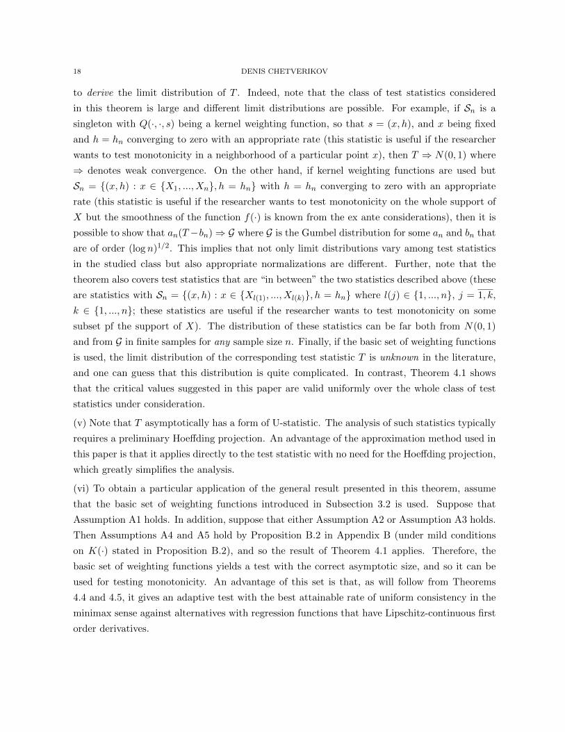
(vii) The theorem can be extended to cover more general versions of the test statistic T . In
particular, the theorem continues to hold if the test statistic T is replaced by
T = T ({Xi, Yi}, {σi},Sn) = maxs∈Sn
w({Xi}, s)b({Xi, Yi}, s)√V ({Xi}, {σi}, s)
where for some c, C > 0, w({Xi}, ·) : Sn → [c, C] is the function that can be used to give unequal
weights to different weighting functions (if T is used, then critical values should be calculated
using T (·, ·, ·) as well). This gives the researcher additional flexibility to incorporate information
on what weighting functions are more important ex ante.
(viii) Finally, the theorem can be extended by equicontinuity arguments to cover certain cases
with infinite Sn where maximum over infinite set of weighting functions in the test statistic T
can be well approximated by maximum over some finite set of weighting functions. Note that
since p in the theorem can be large, approximation is typically easy to achieve. In particular,
if X is the support of X, X has positive Lebesgue measure, the distribution of X is absolutely
continuous with respect to Lebesgue measure on X , and the density of X is bounded below
from zero and from above on X , then the theorem holds with kernel weighting functions and
Sn = {(x, h) : x ∈ X , h ∈ Hn} where Hn = {h = hmaxul : h > hmin, l = 0, 1, 2, . . . }, hmax = C
and hmin = chmax(log n/n)1/3 for some c, C > 0. I omit the proof for brevity. Note, however, that
using this set of weighting functions would require knowledge of the support X (or some method
to estimate it). In addition, taking maximum in the test statistic T would require using some
optimization methods whereas for the basic set of weighting functions, where the maximum is
taken only over Cn log n points for some C > 0, calculating the test statistic T is computationally
straightforward. �
Let sl = inf{support of X} and sr = sup{support of X}. To prove consistency of the test and
to derive the rate of consistency against one-dimensional alternatives, I will also incorporate the
following assumptions.
A6. For any interval [x1, x2] ⊂ [sl, sr], P(X ∈ [x1, x2]) > 0.
This is a mild assumption stating that the support of X is the interval [sl, sr] and that for any
subinterval of the support, there is a positive probability that X belongs to this interval. Let c2
and C2 be strictly positive constants.
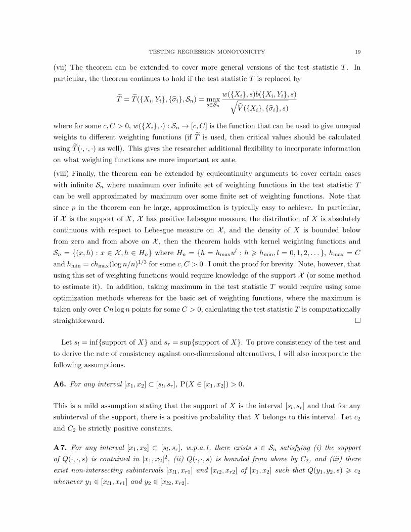
A7. For any interval [x1, x2] ⊂ [sl, sr], w.p.a.1, there exists s ∈ Sn satisfying (i) the support
of Q(·, ·, s) is contained in [x1, x2]2, (ii) Q(·, ·, s) is bounded from above by C2, and (iii) there
exist non-intersecting subintervals [xl1, xr1] and [xl2, xr2] of [x1, x2] such that Q(y1, y2, s) > c2
whenever y1 ∈ [xl1, xr1] and y2 ∈ [xl2, xr2].
20 DENIS CHETVERIKOV
This assumption is satisfied, for example, if Assumption A6 holds, kernel functions are used,
Sn = {(x, h) : x ∈ {X1, . . . , Xn}, h ∈ Hn} where Hn = {h = hmaxul : h > hmin, l = 0, 1, 2, . . . },hmax is bounded below from zero, and hmin → 0.
Let M1 be a subset of M consisting of all models satisfying Assumptions A6 and A7. Then
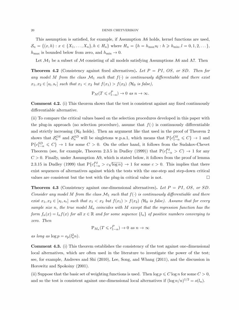
Theorem 4.2 (Consistency against fixed alternatives). Let P = PI, OS, or SD. Then for
any model M from the class M1 such that f(·) is continuously differentiable and there exist
x1, x2 ∈ [sl, sr] such that x1 < x2 but f(x1) > f(x2) (H0 is false),
PM (T 6 cP1−α)→ 0 as n→∞.
Comment 4.2. (i) This theorem shows that the test is consistent against any fixed continuously
differentiable alternative.
(ii) To compare the critical values based on the selection procedures developed in this paper with
the plug-in approach (no selection procedure), assume that f(·) is continuously differentiable
and strictly increasing (H0 holds). Then an argument like that used in the proof of Theorem 2
shows that SOSn and SSDn will be singletons w.p.a.1, which means that P{cOS1−α 6 C} → 1 and
P{cSD1−α 6 C} → 1 for some C > 0. On the other hand, it follows from the Sudakov-Chevet
Theorem (see, for example, Theorem 2.3.5 in Dudley (1999)) that P(cPI1−α > C) → 1 for any
C > 0. Finally, under Assumption A9, which is stated below, it follows from the proof of lemma
2.3.15 in Dudley (1999) that P{cPI1−α > c√
log n} → 1 for some c > 0. This implies that there
exist sequences of alternatives against which the tests with the one-step and step-down critical
values are consistent but the test with the plug-in critical value is not. �
Theorem 4.3 (Consistency against one-dimensional alternatives). Let P = PI, OS, or SD.
Consider any model M from the class M1 such that f(·) is continuously differentiable and there
exist x1, x2 ∈ [sl, sr] such that x1 < x2 but f(x1) > f(x2) (H0 is false). Assume that for every
sample size n, the true model Mn coincides with M except that the regression function has the
form fn(x) = lnf(x) for all x ∈ R and for some sequence {ln} of positive numbers converging to
zero. Then
PMn(T 6 cP1−α)→ 0 as n→∞
as long as log p = op(l2nn).
Comment 4.3. (i) This theorem establishes the consistency of the test against one-dimensional
local alternatives, which are often used in the literature to investigate the power of the test;
see, for example, Andrews and Shi (2010), Lee, Song, and Whang (2011), and the discussion in
Horowitz and Spokoiny (2001).
(ii) Suppose that the basic set of weighting functions is used. Then log p 6 C log n for some C > 0,
and so the test is consistent against one-dimensional local alternatives if (log n/n)1/2 = o(ln).
TESTING REGRESSION MONOTONICITY 21
(iii) Now suppose that kernel weighting functions are used but Sn is a maximal subset of the
basic set such that for any x1, x2, h satisfying (x1, h) ∈ Sn and (x2, h) ∈ Sn, |x2 − x1| > 2h,
and instead of hmin = 0.4hmax(log n/n)1/3 we have hmin → 0 arbitrarily slowly. Then the test
is consistent against one-dimensional local alternatives if n−1/2 = o(ln) (more precisely, for any
sequence ln such that n−1/2 = o(ln), one can choose a sequence hmin = hmin,n satisfying hmin → 0
sufficiently slowly so that the test is consistent). In words, this test is√n-consistent against
such alternatives. I note however, that the practical value of this√n-consistency is limited
because there is no guarantee that for any given sample size n and given deviation from H0,
weighting functions suitable for detecting this deviation are already included in the test statistic.
In contrast, it will follow from Theorem 4.4 that the test based on the basic set of weighting
functions does provide this guarantee. �
Let c3, C3, c4, C4, c5 be strictly positive constants. In addition, let L > 0, β ∈ (0, 1], k > 0, and
hn = (log p/n)1/(2β+3). To derive the uniform consistency rate against the classes of alternatives
with Lipschitz derivatives, Assumptions A6 and A7 will be replaced by the following (stronger)
conditions.
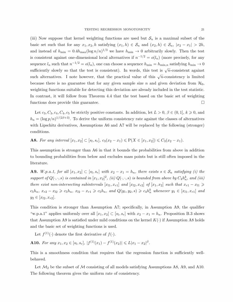
A8. For any interval [x1, x2] ⊂ [sl, sr], c3(x2 − x1) 6 P(X ∈ [x1, x2]) 6 C3(x2 − x1).
This assumption is stronger than A6 in that it bounds the probabilities from above in addition
to bounding probabilities from below and excludes mass points but is still often imposed in the
literature.
A9. W.p.a.1, for all [x1, x2] ⊂ [sl, sr] with x2 − x1 = hn, there exists s ∈ Sn satisfying (i) the
support of Q(·, ·, s) is contained in [x1, x2]2, (ii) Q(·, ·, s) is bounded from above by C4hkn, and (iii)
there exist non-intersecting subintervals [xl1, xr1] and [xl2, xr2] of [x1, x2] such that xr1 − xl1 >c5hn, xr2 − xl2 > c5hn, xl2 − xr1 > c5hn, and Q(y1, y2, s) > c4h
kn whenever y1 ∈ [xl1, xr1] and
y2 ∈ [xl2, xr2].
This condition is stronger than Assumption A7; specifically, in Assumption A9, the qualifier
“w.p.a.1” applies uniformly over all [x1, x2] ⊂ [sl, sr] with x2 − x1 = hn. Proposition B.3 shows
that Assumption A9 is satisfied under mild conditions on the kernel K(·) if Assumption A8 holds
and the basic set of weighting functions is used.
Let f (1)(·) denote the first derivative of f(·).
A10. For any x1, x2 ∈ [sl, sr], |f (1)(x1)− f (1)(x2)| 6 L|x1 − x2|β.
This is a smoothness condition that requires that the regression function is sufficiently well-
behaved.
LetM2 be the subset ofM consisting of all models satisfying Assumptions A8, A9, and A10.
The following theorem gives the uniform rate of consistency.
22 DENIS CHETVERIKOV
Theorem 4.4 (Uniform consistency rate). Let P = PI, OS, or SD. Consider any sequence
of positive numbers {ln} such that ln → ∞, and let M2n denote the subset of M2 consisting of
all models such that the regression function f satisfies infx∈[sl,sr] f(1)(x) < −ln(log p/n)β/(2β+3).
Then
supM∈M2n
PM (T 6 cP1−α)→ 0 as n→∞.
Comment 4.4. (i) Theorem 4.4 gives the rate of uniform consistency of the test against classes
of functions with Lipschitz-continuous first order derivative with Lipschitz constant L and order
β. Importance of uniform consistency against sufficiently large classes of alternatives like those
considered here was previously emphasized in Horowitz and Spokoiny (2001). Intuitively, it
guarantees that there are no reasonable alternatives against which the test has low power if the
sample size is sufficiently large.
(ii) Theorem 4.4 shows that plug-in, one-step, and step-down critical values yield tests with the
same rate of uniform consistency. Nonetheless, it does not mean that the selection procedures
used in one-step and step-down critical values yield no power improvement in comparison with
plug-in critical value. Specifically, it was shown in Comment 4.2 that there exist sequences of
alternatives against which tests with one-step and step-down critical values are consistent but
the test with the plug-in critical value is not.
(iii) Suppose that Sn consists of the basic set of weighting functions. In addition, suppose that
Assumptions A1 and A8 are satisfied. Further, suppose that either Assumption A2 or A3 is
satisfied. Then Assumptions A4 and A5 hold by Proposition B.2 and Assumption A9 holds by
Proposition B.3 under mild conditions on the kernel K(·). Then Theorem 4.4 implies that the
test with this set of weighting functions is uniformly consistent against classes of functions with
Lipschitz-continuous first order derivative with Lipschitz order β whenever infx∈[sl,sr] f(1)n (x) <
−ln(log n/n)β/(2β+3) for some ln →∞. On the other hand, it will be shown in Theorem 4.5 that
no test can be uniformly consistent against models with infx∈[sl,sr] f(1)n (x) > −C(log n/n)β/(2β+3)
for some sufficiently small C > 0 if it controls size, at least asymptotically. Therefore, the test
based on the basic set of weighting functions is rate optimal in the minimax sense.
(iv) Note that the test is rate optimal in the minimax sense simultaneously against classes of
functions with Lipschitz-continuous first order derivative with Lipschitz order β for all β ∈ (0, 1].
In addition, implementing the test does not require the knowledge of β. For these reasons, the
test with the basic set of weighting functions is called adaptive and rate optimal. �
To conclude this section, I present a theorem that gives a lower bound on the possible rates
of uniform consistency against the class M2 so that no test that maintains asymptotic size can
have a faster rate of uniform consistency. Let ψ = ψ({Xi, Yi}) be a generic test. In other words,
TESTING REGRESSION MONOTONICITY 23
ψ({Xi, Yi}) is the probability that the test rejects upon observing the data {Xi, Yi}. Note that
for any deterministic test ψ = 0 or 1.
Theorem 4.5 (Lower bound on possible consistency rates). For any test ψ satisfying EM [ψ] 6
α + o(1) as n → ∞ for all models M ∈ M2 such that H0 holds, there exists a sequence of
models M = Mn belonging to the class M2 such that f(·) = fn(·) satisfies infx∈[sl,sr] f(1)n (x) <
−C(log n/n)β/(2β+3) for some sufficiently small constant C > 0 and EMn [ψ] 6 α+o(1) as n→∞.
Here EMn [·] denotes the expectation under the distributions of the model Mn.
Comment 4.5. This theorem shows that no test can be uniformly consistent against models
with infx∈[sl,sr] f(1)n (x) > −C(log n/n)β/(2β+3) for some sufficiently small C > 0 if it controls size,
at least asymptotically. �
5. Models with Multiple Covariates
Most empirical studies contain additional covariates that should be controlled for. In this
section, I extend the results presented in Section 4 to allow for this possibility. I consider cases
of both nonparametric and partially linear models. For brevity, I will only consider the results
concerning size properties of the test. The power properties can be obtained using the arguments
closely related to those used in Theorems 4.2, 4.3, and 4.4.
5.1. Multivariate Nonparametric Model. In this subsection, I consider a general nonpara-
metric regression model, so that the model is given by
Y = f(X,Z) + ε (17)
where Y is a scalar dependent random variable, X a scalar independent random variable, Z a
vector in Rd of additional independent random variables that should be controlled for, f(·) an
unknown function, and ε an unobserved scalar random variable satisfying E[ε|X,Z] = 0 almost
surely.
Let Sz be some subset of Rd. The null hypothesis, H0, to be tested is that for any x1, x2 ∈ Rand z ∈ Sz, f(x1, z) 6 f(x2, z) whenever x1 6 x2. The alternative, Ha, is that there are
x1, x2 ∈ R and z ∈ Sz such that x1 < x2 but f(x1, z) > f(x2, z). The decision is to be made
based on the i.i.d. sample of size n, {Xi, Zi, Yi}16i6n from the distribution of (X,Z, Y ).
The choice of the set Sz is up to the researcher and has to be made depending on the hypothesis
to be tested. For example, if Sz = Rd, then H0 means that the function f(·) is increasing in
the first argument for all values of the second argument. If the researcher is interested in one
particular value, say z0, then she can set Sz = z0, which will mean that under H0, the function
f(·) is increasing in the first argument when the second argument equals z0.
24 DENIS CHETVERIKOV
The advantage of the nonparametric model studied in this subsection is that it is fully flexible
and, in particular, allows for heterogeneous effects of X on Y . On the other hand, the nonpara-
metric model suffers from the curse of dimensionality and may result in tests with low power if
the researcher has many additional covariates. In this case, it might be better to consider the
partially linear model studied below.
To define the test statistic, let Sn be some general set that depends on n and is (implicitly)
allowed to depend on {Xi, Zi}. In addition, let z : Sn → Sz and ` : Sn → (0,∞) be some
functions, and for s ∈ Sn, let Q(·, ·, ·, ·, s) : R×R×Rd×Rd → R be weighting functions satisfying
Q(x1, x2, z1, z2, s) = Q(x1, x2, s)K
(z1 − z(s)`(s)
)K
(z2 − z(s)`(s)
)for all x1, x2, z1, and z2 where the functions Q(·, ·, s) satisfy Q(x1, x2, s) = Q(x2, x1, s) and
Q(x1, x2, s) > 0 for all x1 and x2. For example, Q(·, ·, s) can be a kernel weighting function.
The functions Q(·, ·, ·, ·, s) are also (implicitly) allowed to depend on {Xi, Zi}. Here K : Rd → Ris some positive compactly supported auxiliary kernel function, and `(s), s ∈ Sn, are auxiliary
bandwidth values. Intuitively, Q(·, ·, ·, ·, s) are local-in-z(s) weighting functions. It is important
here that the auxiliary bandwidth values `(s) depend on s. For example, if kernel weighting
functions are used, so that s = (x, h, z, `), then one has to choose h = h(s) and ` = `(s) so
that nh`d+2 = op(1/ log p) and 1/(nh`d) 6 Cn−c w.p.a.1 for some c, C > 0 uniformly over all
s = (x, h, z, `) ∈ Sn; see discussion below.
Further, let
b(s) = b({Xi, Zi, Yi}, s) = (1/2)∑
16i,j6n
(Yi − Yj)sign(Xj −Xi)Q(Xi, Xj , Zi, Zj , s) (18)
be a test function. Conditional on {Xi, Zi}, the variance of b(s) is given by
V (s) = V ({Xi, Zi}, {σi}, s) =∑
16i6n
σ2i
∑16j6n
sign(Xj −Xi)Q(Xi, Xj , Zi, Zj , s)
2
(19)
where σi = (E[ε2i |Xi, Zi])
1/2, and estimated variance is
V (s) = V ({Xi, Zi}, {σi}, s) =∑
16i6n
σ2i
∑16j6n
sign(Xj −Xi)Q(Xi, Xj , Zi, Zj , s)
2
(20)
where σi is some estimator of σi. Then the test statistic is
T = T ({Xi, Zi, Yi}, {σi},Sn) = maxs∈Sn
b({Xi, Zi, Yi}, s)√V ({Xi, Zi}, {σi}, s)
.
Large values of T indicate that H0 is violated. The critical value for the test can be calculated
using any of the methods described in Section 3. For example, the plug-in critical value is defined
TESTING REGRESSION MONOTONICITY 25
as the conditional (1−α) quantile of T ? = T ({Xi, Zi, Y?i }, {σi},Sn) given {Xi, Zi}, {σi}, and Sn
where Y ?i = σiεi for i = 1, n.
Let cPI1−α, cOS1−α, and cSD1−α denote the plug-in, one-step, and step-down critical values, respec-
tively. In addition, let
An = maxs∈Sn
max16i6n
∣∣∣∣∣∣∑
16j6n
sign(Xj −Xi)Q(Xi, Xj , Zi, Zj , s)/(V (s))1/2
∣∣∣∣∣∣ (21)
be a sensitivity parameter. Recall that p = |Sn|. To prove the result concerning multivariate
nonparametric model, I will impose the following condition.
A11. (i) `(s)∑
16i,j6nQ(Xi, Xj , Zi, Zj , s)/(V (s))1/2 = op(1/√
log p) uniformly over s ∈ Sn, and
(ii) the regression function f has uniformly bounded first order partial derivatives.
Discussion of this assumption is given below. In addition, I will need to modify Assumptions
A1, A2, and A5:
A1′ (i) P(|ε| > u|X,Z) 6 exp(−u/C1) for all u > 0 and σi > c1 for all i = 1, n.
A2′ (i) σi = Yi − f(Xi, Zi) for all i = 1, n and (ii) f(Xi, Zi) − f(Xi, Zi) = op(n−κ1) uniformly
over i = 1, n.
A5′ (i) An(log(pn))7/2 = op(1), (ii) if A2′ holds, then log p/n(1/4)∧κ1∧κ3 = op(1), and if A3 holds,
then log p/nκ2∧κ3 = op(1).
Assumption A1′ imposes the restriction that εi’s have sub-exponential tails, which is stronger
than Assumption A1. It holds, for example, if εi’s have normal distribution or εi’s are uniformly
bounded in absolute value. Assumption A2′ is a simple extension of Assumption A2 to account for
the vector of additional covariates Z. Further, assume that Q(·, ·, s) is a kernel weighting function
for all s ∈ Sn, so that s = (x, h, z, `), the joint density of X and Z is bounded below from zero
and from above on its support, and h > ((log n)2/(Cn))1/(d+1) and ` > ((log n)2/(Cn))1/(d+1)
w.p.a.1 for some C > 0 uniformly over all s = (x, h, z, `) ∈ Sn. Then it follows as in the proof of
Proposition B.2, that A11-i holds if nh`d+2 = op(1/ log p) uniformly over all s = (x, h, z, `) ∈ Snand that A5′-i holds if 1/(nh`d) 6 Cn−c w.p.a.1 for some c, C > 0 uniformly over all s =
(x, h, z, `) ∈ Sn.
The key difference between the multivariate case studied in this section and univariate case
studied in Section 4 is that now it is not necessarily the case that E[b(s)] 6 0 underH0. The reason
is that it can be the case under H0 that f(x1, z1) > f(x2, z2) even if x1 < x2 unless z1 = z2. This
yields a bias term in the test statistic. Assumption A11 ensures that this bias is asymptotically
negligible relative to the concentration rate of the test statistic. The difficulty, however, is that
this assumption contradicts the condition nA4n(log(pn))7 = op(1) imposed in Assumption A5 and
26 DENIS CHETVERIKOV
used in the theory for the case when Z is absent. Indeed, under the assumptions specified in
the paragraph above, the condition nA4n(log(pn))7 = op(1) requires 1/(nh2`2d) = op(1) uniformly
over all s = (x, h, z, `) ∈ Sn, which is impossible if nh`d+2 = op(1/ log p) uniformly over all
s = (x, h, z, `) ∈ Sn and d > 2. To deal with this problem, I have to relax Assumption A5. This
in turn requires imposing stronger conditions on the moments of ε. For these reasons, I replace
Assumption A1 by A1′. This allows me to apply a powerful method developed in Chernozhukov,
Chetverikov, and Kato (2012) and replace Assumption A5 by A5′.
Let MNP denote the set of models given by equation (17), function f(·), joint distribution of
X, Z, and ε satisfying E[ε|X,Z] = 0 almost surely, weighting functions Q(·, ·, ·, ·, s) for s ∈ Sn(possibly depending on Xi’s and Zi’s), and estimators {σi} such that uniformly over this class, (i)
Assumptions A1′, A4, A5′, and A11 are satisfied (where V (s), V (s), and An are defined in (19),
(20), and (21), respectively), and (ii) either Assumption A2′ or A3 is satisfied. The following
theorem shows that the test in the multivariate nonparametric model controls asymptotic size.
Theorem 5.1 (Size properties in the multivariate nonparametric model). Let P = PI, OS, or
SD. Let MNP,0 denote the set of all models M ∈MNP satisfying H0. Then
infM∈MNP,0
PM (T 6 cP1−α) > 1− α+ o(1) as n→∞.
In addition, let MNP,00 denote the set of all models M ∈ MNP,0 such that f(x) = C for some
constant C and all x ∈ R. Then
supM∈MNP,00
PM (T 6 cP1−α) = 1− α+ o(1) as n→∞.
Comment 5.1. (i) The result of this theorem is new and I am not aware of any similar or
related result in the literature. Here I briefly comment on difficulties arising if one tries to
obtain a result like that in Theorem 5.1 by applying proof techniques that were previously used
in the literature for the model where Z is absent. The approach of Ghosal, Sen, and van der
Vaart (2000) consists of first providing a Gaussian coupling (strong approximation) for the whole
process {b(s)/V (s) : s ∈ Sn} and then employing results of the extreme value theory of Gaussian
processes with one-dimensional domain (see, for example, Leadbetter, Lindgren, and Rootzen
(1983) for a detailed description of these results) to derive a limit distribution of suprema of
these processes. When Z is present, however, one has to apply the results of the extreme value
theory for Gaussian processes with multi-dimensional domain (these processes are refered in the
literature as Gaussian random fields); see Piterbarg (1996). Although there do exist important
applications of this theory in econometrics (see, for example, Lee, Linton, and Whang (2009)),
it is not clear how to apply it in the setting like that studied in this section where the covariance
structure of the process {{b(s)/V (s) : s ∈ Sn} is rather complicated, which is the case when kernel
weighting functions are used with many different bandwidth values. Hall and Heckman (2000)
take a different approach: they first provide a Gaussian coupling and then use integration by
TESTING REGRESSION MONOTONICITY 27
parts of stochastic integrals to show validity of their critical values. Even when Z is absent, they
proved their results only when Xi’s are equidistant on some interval, but, more importantly, it is
also unclear how to generalize their techniques based on integration by parts to multi-dimensional
setting.
(ii) There are other possible notions of monotonicity in the multivariate model (17). Assume,
for simplicity, that both X and Z are scalars. Then one might want to test the null hypothesis,
H0, that f(x2, z2) > f(x1, z1) for all x1, x2, z1, and z2 satisfying x2 > x1 and z2 > z1 against
the alternative, Ha, that there exist x1, x2, z1, and z2 such that x2 > x1 and z2 > z1 but
f(x2, z2) < f(x1, z1). To test this H0, one can consider the following test functions:
b(s) = (1/2)∑
16i,j6n
(Yi − Yj)sign(Xj −Xi)I{Zj > Zi}Q(Xi, Xj , Zi, Zj , s)
where the function Q satisfies Q(x1, x2, z1, z2, s) > 0 for all x1, x2, z1, z2, and s. Note that there
is no bias term present in the test function, and so one does not have to consider local-in-z
weighting functions. The theory for this problem can be obtained along the same line as that
used in Section 4.
(iii) The same techniques that I use to test monotonicity in this paper can also be used to
test other hypotheses that are of interest in economic theory. For example, one can test that
the function f(·, ·) has increasing differences or super-modularity property. It is said that the
function f(·, ·) has increasing differences or super-modularity property if for all x1 < x2, f(x2, z)−f(x1, z) is increasing in z. This property plays an important role in Robust comparative statics.
Specifically, one can obtain a testing procedure based on the following test functions:
b(s) =∑
16j,k,l,m6n
((Yj − Yk)− (Yl − Ym))Q(Xj , Xk, Xl, Xm, Zj , Zk, Zl, Zm, s)
where the function Q can take the form of kernel weighting function:
Q(x1, x2, x3, x4, z1, z2, z3, z4, s)
= K
(x1 − xr(s)
h(s)
)K
(x2 − xl(s)h(s)
)K
(x3 − xr(s)
h(s)
)K
(x4 − xl(s)h(s)
)×K
(z1 − zr(s)h(s)
)K
(z2 − zr(s)h(s)
)K
(z3 − zl(s)h(s)
)K
(z4 − zl(s)h(s)
)and s = (xl, xr, zl, zr, h) with xr > xl and zr > zl and some bandwidth value h. �
5.2. Partially Linear Model. In this model, additional covariates enter the regression function
as additively separable linear form. Specifically, the model is given by
Y = f(X) + ZTβ + ε (22)
where Y is a scalar dependent random variable, X a scalar independent random variable, Z a
vector in Rd of additional independent random variables that should be controlled for, f(·) an
28 DENIS CHETVERIKOV
unknown function, β a vector in Rd of unknown parameters, and ε an unobserved scalar random
variable satisfying E[ε|X,Z] = 0 almost surely. As in Section 4, the problem is to test the null
hypothesis, H0, that f(·) is nondecreasing against the alternative, Ha, that there are x1 and x2
such that x1 < x2 but f(x1) > f(x2). The decision is to be made based on the i.i.d. sample
of size n, {Xi, Zi, Yi}16i6n from the distribution of (X,Z, Y ). The regression function f(·) is
assumed to be smooth but I do not impose any parametric structure on it.
An advantage of the partially linear model over the fully nonparametric model is that it does
not suffer from the curse of dimensionality, which decreases the power of the test and may be
a severe problem if the researcher has many additional covariates to control for. On the other
hand, the partially linear model does not allow for heterogeneous effects of the factor X, which
might be restrictive in some applications. It is necessary to have in mind that the test obtained
for the partially linear model will be inconsistent if this model is misspecified.
Let me now describe the test. The main idea is to estimate β by some βn and to apply the
methods described in Section 3 for the dataset {Xi, Yi − ZTi βn}. For example, one can take an
estimator of Robinson (1988), which is given by
βn =
(n∑i=1
ZiZTi
)−1( n∑i=1
ZiYi
)where Zi = Zi − E[Z|X = Xi], Yi = Yi − E[Y |X = Xi], and E[Z|X = Xi] and E[Y |X =
Xi] are nonparametric estimators of E[Z|X = Xi] and E[Y |X = Xi], respectively. Define
Yi = Yi − ZTi βn, and let the test statistic be T = T ({Xi, Yi}, {σi},Sn) where T (·, ·, ·) is defined
in (5) and estimators σi of σi = (E[ε2i |Xi])
1/2 (here εi = Yi − f(Xi) − ZTi β) satisfy either
σi = εi = Yi−f(Xi)−ZTi βn (here f(Xi) is some estimator of f(Xi), which is uniformly consistent
over i = 1, n) or σi is some uniformly consistent estimator of σi. The critical value for the test is
simulated by one of the methods (plug-in, one-step, or step-down) described in Section 3 using
the data {Xi, Yi}, estimators {σi}, and the set of weighting functions Sn. As in Section 3, let
cPI1−α, cOS1−α, and cSD1−α denote the plug-in, one-step, and step-down critical values, respectively.
Let C5 > 0 be some constant. To obtain results for partially linear models, I will impose the
following condition.
A12. (i) ‖Z‖ 6 C5 almost surely, (ii) ‖βn−β‖ = Op(n−1/2), and (iii) uniformly over all s ∈ Sn,∑
16i,j6nQ(Xi, Xj , s)/V (s)1/2 = op(√n/ log p).
The assumption that the vector Z is bounded is a mild regularity condition and can be easily
relaxed. Further, Horowitz (2009) provides a set of conditions so that ‖βn − β‖ = Op(n−1/2)
when βn is the Robinson’s estimator. Finally, it follows from the proof of Proposition B.2 that
under Assumption A8, Assumption A12-iii is satisfied if kernel weighting functions are used as
long as hmax = op(1/ log p) and hmin > (log n)2/(Cn) w.p.a.1. for some C > 0. In addition, I will
TESTING REGRESSION MONOTONICITY 29
need to modify Assumption A2 to account for the presence of the vector of additional covariates
Z:
A2′′ (i) σi = Yi − f(Xi) − ZTi βn for all i = 1, n and (ii) f(Xi) − f(Xi) = op(n−κ1) uniformly
over i = 1, n.
Let MPL be a class of models given by equation (22), function f(·), parameter β, joint
distribution of X, Z, and ε satisfying E[ε|X,Z] = 0 almost surely, weighting functions Q(·, ·, s)for s ∈ Sn (possibly depending on Xi’s), an estimator βn, and estimators {σi} such that uniformly
over this class, (i) Assumptions A1, A4, A5, and A12 are satisfied (where V (s), V (s), and An
are defined in (3), (4), and (16), respectively), and (ii) either Assumption A2′′ or A3 is satisfied.
The size properties of the test are given in the following theorem.
Theorem 5.2 (Size properties in the partially linear model). Let P = PI, OS, or SD. Let
MPL,0 denote the set of all models M ∈MPL satisfying H0. Then
infM∈MPL,0
PM (T 6 cP1−α) > 1− α+ o(1) as n→∞.
In addition, let MPL,00 denote the set of all models M ∈ MPL,0 such that f(x) = C for some
constant C and all x ∈ R. Then
supM∈MPL,00
PM (T 6 cP1−α) = 1− α+ o(1) as n→∞.
Comment 5.2. The result of Theorem 5.2 can be extended to cover a general separately additive
models. Specifically, assume that the data come from the model
Y = f(X) + g(Z) + ε (23)
where g(·) is some unknown smooth function and all other notation is the same as above. Then
one can testH0 that f(·) is nondecreasing against the alternativeHa that there are x1 and x2 such
that x1 < x2 but f(x1) > f(x2) using a method similar to that used above with the exception
that now Yi = Yi − g(Zi) where g(Zi) is some nonparametric estimator of g(Zi). Specifically,
consider the following conditions:
A2′′′ (i) σi = Yi − f(Xi) − g(Zi) for all i = 1, n and (ii) f(Xi) − f(Xi) = op(n−κ1) uniformly
over i = 1, n.
A12′ (i) max16i6n |g(Zi) − g(Zi)| = Op(ψ−1n ) for some sequence ψn → ∞, and (ii) uniformly
over all s ∈ Sn,∑
16i,j6nQ(Xi, Xj , s)/V (s)1/2 = op(√ψn/ log p).
Let MSA, MSA,0, and MSA,00 denote sets of models that are defined as MPL, MPL,0, and
MPL,00 with (22) and Assumptions A12 and A2′′ replaced by (23) and Assumptions A12′ and
A2′′′. Then Theorem 5.2 applies withMPL,MPL,0, andMPL,00 replaced byMSA,MSA,0, and
30 DENIS CHETVERIKOV
MSA,00. This result can be proven from the argument similar to that used to prove Theorem
5.2. �
6. Models with Endogenous Covariates
Empirical studies in economics often contain endogenous covariates. Therefore, it is important
to extend the results on testing monotonicity obtained in this paper to cover this possibility.
Allowing for endogenous covariates in nonparametric settings like the one considered here is
challenging and several approaches have been proposed in the literature. In this paper, I consider
the approach proposed in Newey, Powell, and Vella (1999). In their model,
Y = f(X) +W, (24)
X = λ(U) + Z (25)
where Y is a scalar dependent variable, X a scalar covariate, U a vector in Rd of instruments,
f(·) and λ(·) unknown functions, and W and Z unobserved scalar random variables satisfying
E[W |U,Z] = E[W |Z] and E[Z|U ] = 0 (26)
almost surely. In this setting, X is endogenous in the sense that equation E[W |X] = 0 almost
surely does not necessarily hold. The problem is to test the null hypothesis, H0, that f(·) is
nondecreasing against the alternative, Ha, that there are x1 and x2 such that x1 < x2 but
f(x1) > f(x2). The decision is to be made based on the i.i.d. sample of size n, {Xi, Ui, Yi}16i6nfrom the distribution of (X,U, Y ).
It is possible to consider a more general setting where the function f of interest depends on
X and U1, that is Y = f(X,U1) + ε and U = (U1, U2) but I refrain from including additional
covariates for brevity.
An alternative to the model defined in (24)-(26) is the model defined by (24) and
E[W |U ] = 0 (27)
almost surely. Newey, Powell, and Vella (1999) noted that neither model is more general than
the other one. The reason is that it does not follow from (26) that (27) holds, and it does not
follow from (27) that (26) holds. Both models have been used in the empirical studies. The
latter model have been studied in Newey and Powell (2003), Hall and Horowitz (2005), Blundell,
Chen, and Kristensen (2007), and Darolles el. al. (2011), among many others.
Let me now get back to the model defined by (24)-(26). A key observation of Newey, Powell,
and Vella (1999) is that in this model,
E[Y |U,Z] = E[f(X)|U,Z] + E[W |U,Z] = E[f(X)|U,X] + E[W |Z] = f(X) + g(Z)
TESTING REGRESSION MONOTONICITY 31
where g(z) = E[W |Z = z]. This implies that
E[Y |X,Z] = f(X) + g(Z). (28)
Therefore, the regression function of Y on X and Z is separately additive in X and Z, and so, if
Zi = Xi−λ(Ui)’s were known, both f(·) and g(·) could be estimated by one of the nonparametric
methods suitable for estimating separately additive models. One particularly convenient method
to estimate such models is a series estimator. Further, note that even though Zi’s are unknown,
they can be consistently estimated from the data as residuals from the nonparametric regression
of X on U . Then one can estimate both f(·) and g(·) by employing a nonparametric method for
estimating separately additive models with Zi’s replaced by their estimates. Specifically, let Zi =
Xi − E[X|U = Ui] where E[X|U = Ui] is a consistent nonparametric estimator of E[X|U = Ui].
Further, for an integer L > 0, let rL,f (x) = (rf1L(x), ..., rfLL(x))′ and rL,g(z) = (rg1L(z), ..., rgLL(z))′
be vectors of approximating functions for f(·) and g(·), respectively, so that
f(x) ≈ rL,f (x)′βf and g(z) ≈ rL,g(z)′βg
for L large enough where βf and βg are vectors in RL of coefficients. In addition, let rL(x, z) =
(rL,f (x)′, rL,g(z)′)′ and R = (rL(X1, Z1), ..., rL(Xn, Zn)). Then the OLS estimator of βf and βg
is (βf
βg
)=(R′R
)−1 (R′Y n
1
)where Y n
1 = (Y1, ..., Yn)′, and the series estimators f(x) and g(x) of f(x) and g(z) are rL,f (x)′βf
and rL,g(z)′βg for all x and z, respectively.
Now, it follows from (28) that
Y = f(X) + g(Z) + ε
where E[ε|X,Z] = 0 almost surely. This is exactly the model discussed in Comment 5.2, and
since I have an estimator of g(·), it is possible to test H0 using the same ideas as in Comment 5.2.
Specifically, let Yi = Y −g(Zi) and apply a test described in Section 3 with the data {Xi, Yi}16i6n;
that is, let the test statistic be T = T ({Xi, Yi}, {σi},Sn) where the function T (·, ·, ·) is defined
in (5) and estimators σi of σi = (E[ε2i |Xi])
1/2 (here εi = Yi − f(Xi) − g(Zi)) satisfy either
σi = εi = Yi − f(Xi) − g(Zi) or σi is some uniformly consistent estimator of σi. Let cPI1−α,
cOS1−α, and cSD1−α denote the plug-in, one-step, and step-down critical values, respectively, that
are obtained as in Section 3 using the data {Xi, Yi}, estimators {σi}, and the set of weighting
functions Sn.
To obtain results for this testing procedure, I will use the following modifications of Assump-
tions A2′′′ and A12′:
A2′′′′ (i) σi = Yi − f(Xi) − g(Zi) for all i = 1, n and (ii) f(Xi) − f(Xi) = op(n−κ1) uniformly
over i = 1, n.

32 DENIS CHETVERIKOV
A12′′ (i) max16i6n |g(Zi) − g(Zi)| = Op(ψ−1n ) for some sequence ψn → ∞, and (ii) uniformly
over all s ∈ Sn,∑
16i,j6nQ(Xi, Xj , s)/V (s)1/2 = op(√ψn/ log p).
Assumption A2′′′′ is a simple extension of Assumption A2′′′ that takes into account that Zi’s
have to be estimated by Zi’s. Further, Assumption A12′′ requires that max16i6n |g(Zi)−g(Zi)| =Op(ψ
−1n ) for some sequence ψn →∞. For the estimator g(·) of g(·) described above, this require-
ment follows from Lemma 4.1 and Theorem 4.3 in Newey, Powell, and Vella (1999) who also
provide certain primitive conditions for this requirement to hold. Specific choices of ψn depend
on how smooth the functions f(·) and g(·) are and how the number of series terms, L, is chosen.
Let MEC be a class of models given by equations (24)-(26), functions f(·) and λ(·), joint
distribution of X, U , W , and Z, weighting functions Q(·, ·, s) for s ∈ Sn (possibly depending on
Xi’s), an estimator g(·) of g(·), and estimators {σi} of {σi} such that uniformly over this class,
(i) Assumptions A1, A4, A5, and A12′′ are satisfied (where V (s), V (s), and An are defined in
(3), (4), and (16), respectively), and (ii) either Assumption A2′′′′ or A3 is satisfied.
Theorem 6.1 (Size properties in the model with endogenous covariates). Let P = PI, OS, or
SD. Let MEC,0 denote the set of all models M ∈MEC satisfying H0. Then
infM∈MEC,0
PM (T 6 cP1−α) > 1− α+ o(1) as n→∞.
In addition, let MEC,00 denote the set of all models M ∈ MEC,0 such that f ≡ C for some
constant C. Then
supM∈MEC,00
PM (T 6 cP1−α) = 1− α+ o(1) as n→∞.
Comment 6.1. Around the same time this paper became publicly available, Gutknecht (2013)
obtained a test of monotonicity of the function f(·) in the same model (24)-(26). The test in that
paper is a special case of the class of tests derived in this paper. Specifically, Gutknecht (2013)
obtained a test based on test functions (7). The major difference, however, is that his test is not
adaptive because it is based on one non-stochastic bandwidth value. �
7. Sample Selection Models
It is widely recognized in econometrics literature that sample selection problems can result
in highly misleading inference in otherwise standard regression models. The purpose of this
section is to briefly show that the same techniques that are used in the last section to deal
with endogeneity issues can also be used to deal with sample selection issues. For concreteness, I
consider a nonparametric version of the classical Heckman’s sample selection model; see Heckman
(1979). The nonparametric version of the Heckman’s model was previously analyzed in great
TESTING REGRESSION MONOTONICITY 33
generality in Das, Newey, and Vella (2003). Specifically, I consider the model
Y ∗ = f(X) +W, (29)
Y = DY ∗ (30)
where Y ∗ is an unobserved scalar dependent random variable, Y a scalar random variable, X a
covariate, D a binary selection indicator, W unobserved scalar random variable. The problem
in this model arises when W is not independent of D. To deal with this problem, let Z denote
a vector of random variables that affect selection D, and let p(x, z) = E[D|X = x, Z = z] be the
propensity score. Further, assume that Z is such that
E[W |X,Z,D = 1] = λ(p(X,Z)) (31)
where λ(·) is some unknown function. This condition is reasonable in many settings; see, in
particular, discussion on p.35 of Das, Newey, and Vella (2003). I am interested in testing the
null hypothesis that the function f(·) in the model (29)-(31) is weakly increasing against the
alternative that it is not weakly increasing based on the random sample {Xi, Zi, Yi}16i6n from
the distribution of (X,Z, Y ).
A key observation of Das, Newey, and Vella (2003) is that under (31), equations (29) and (30)
imply that
E[Y |X,Z,D = 1] = f(X) + λ(p(X,Z)),
and so denoting P = p(X,Z),
E[Y |X,P,D = 1] = f(X) + λ(P ). (32)
Therefore, if Pi = p(Xi, Zi)’s were known, one could estimate both f(·) and λ(·) by one of
the nonparametric methods suitable for estimating separately additive models applied to the
regression of Y on X and P based on the subsample of observations with Di = 1. Further, note
that even though Pi’s are unknown, they can be estimated consistently from the data as the
predicted values in the nonparametric regression of D on X and Z. Hence, one can estimate
both f(·) and λ(·) by one of the non-parametric methods suitable for estimating additive models
applied to the regression of Y on X and P with Pi’s replaced by Pi’s where Pi = p(Xi, Zi) and
p(·, ·) is a nonparametric estimator of p(·, ·).
Now, (32) implies that
Y = f(X) + λ(P ) + ε
where E[ε|X,P,D = 1] = 0 almost surely. This is exactly the model discussed in Comment 5.2,
and since an estimator λ(·) of λ(·) is available, one can test monotonicity of f(·) by applying the
results in Section 3 with the data {Xi, Yi}16i6n where Yi = Y − λ(Pi). For this test, one can
state the theorem that is analogous to Theorem 6.1.
34 DENIS CHETVERIKOV
8. Monte Carlo Simulations
In this section, I provide results of a small simulation study. The aim of the simulation study
is to shed some light on the size properties of the test in finite samples and to compare its power
with that of other tests developed in the literature. In particular, I consider the tests of Gijbels
et. al. (2000) (GHJK), Ghosal, Sen, and van der Vaart (2000) (GSV), and Hall and Heckman
(2000) (HH).
I consider samples of size n = 100, 200, and 500 with Xi’s uniformly distributed on the [−1, 1]
interval, and regression functions of the form f(x) = c1x− c2φ(c3x) where c1, c2, c3 > 0 and φ(·)is the pdf of the standard normal distribution. I assume that εi is a zero-mean random variable
that is independent of Xi and has the standard deviation σ. Depending on the experiment,
εi has either normal or continuous uniform distribution. Four combinations of parameters are
studied: (1) c1 = c2 = c3 = 0 and σ = 0.05; (2) c1 = c3 = 1, c2 = 4, and σ = 0.05; (3) c1 = 1,
c2 = 1.2, c3 = 5, and σ = 0.05; (4) c1 = 1, c2 = 1.5, c3 = 4, and σ = 0.1. Cases 1 and 2 satisfy
H0 whereas cases 3 and 4 do not. In case 1, the regression function is flat corresponding to the
maximum of the type I error. In case 2, the regression function is strictly increasing. Cases 3
and 4 give examples of the regression functions that are mostly increasing but violate H0 in the
small neighborhood near 0. All functions are plotted in figure 2. The parameters were chosen so
that to have nontrivial rejection probability in most cases (that is, bounded from zero and from
one).
Let me describe the tuning parameters for all tests that are used in the simulations. For the
tests of GSV, GHJK, and HH, I tried to follow their instructions as closely as possible. For the
test developed in this paper, I use kernel weighting functions with k = 0, Sn = {(x, h) : x ∈{X1, ..., Xn}, h ∈ Hn}, and the kernel K(x) = 0.75(1 − x2) for x ∈ (−1; +1) and 0 otherwise.
I use the set of bandwidth values Hn = {hmaxul : h > hmin, l = 0, 1, 2, ...}, u = 0.5, hmax = 1,
hmin = 0.4hmax(log n/n)1/3, and the truncation parameter γ = 0.01. For the test of GSV, I use
the same kernel K with the bandwidth value hn = n−1/5, which was suggested in their paper,
and I consider their sup-statistic. For the test of GHJK, I use their run statistic maximized
over k ∈ {10(j − 1) + 1 : j = 1, 2, ...0.2n} (see the original paper for the explanation of the
notation). For the test of HH, local polynomial estimates are calculated over r ∈ nHn at every
design point Xi. The set nHn is chosen so that to make the results comparable with those for
the test developed in this paper. Finally, I consider two versions of the test developed in this
paper depending on how σi is estimated. More precisely, I consider the test with σi estimated
by the Rice’s method (see equation (11)), which I refer to in the table below as CS (consistent
sigma), and the test with σi = εi where εi is obtained as the residual from estimating f using
the series method with polynomials of order 5, 6 and 8 whenever the sample size n is 100, 200,
and 500, respectively, which I refer to in the table below as IS (inconsistent sigma).
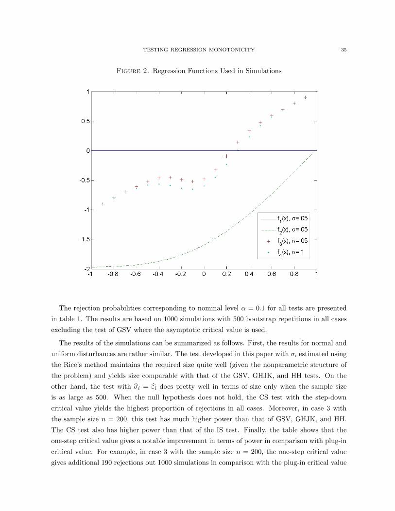
TESTING REGRESSION MONOTONICITY 35
Figure 2. Regression Functions Used in Simulations
The rejection probabilities corresponding to nominal level α = 0.1 for all tests are presented
in table 1. The results are based on 1000 simulations with 500 bootstrap repetitions in all cases
excluding the test of GSV where the asymptotic critical value is used.
The results of the simulations can be summarized as follows. First, the results for normal and
uniform disturbances are rather similar. The test developed in this paper with σi estimated using
the Rice’s method maintains the required size quite well (given the nonparametric structure of
the problem) and yields size comparable with that of the GSV, GHJK, and HH tests. On the
other hand, the test with σi = εi does pretty well in terms of size only when the sample size
is as large as 500. When the null hypothesis does not hold, the CS test with the step-down
critical value yields the highest proportion of rejections in all cases. Moreover, in case 3 with
the sample size n = 200, this test has much higher power than that of GSV, GHJK, and HH.
The CS test also has higher power than that of the IS test. Finally, the table shows that the
one-step critical value gives a notable improvement in terms of power in comparison with plug-in
critical value. For example, in case 3 with the sample size n = 200, the one-step critical value
gives additional 190 rejections out 1000 simulations in comparison with the plug-in critical value
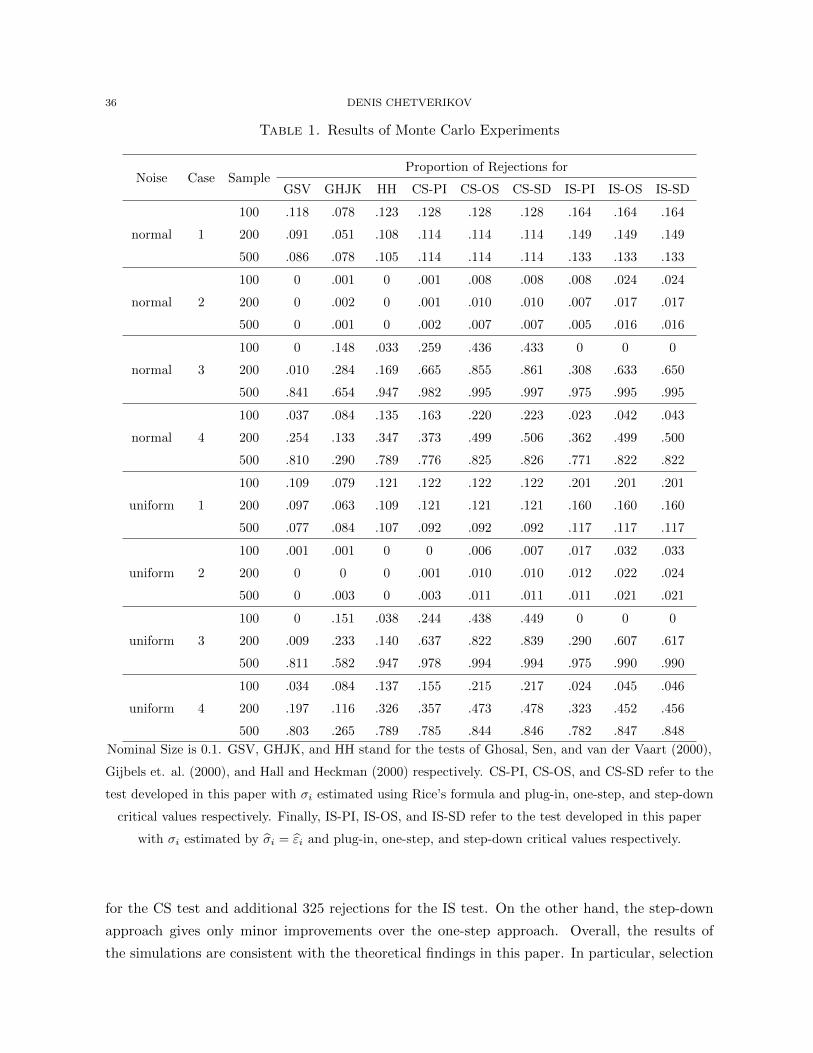
36 DENIS CHETVERIKOV
Table 1. Results of Monte Carlo Experiments
Noise Case SampleProportion of Rejections for
GSV GHJK HH CS-PI CS-OS CS-SD IS-PI IS-OS IS-SD
100 .118 .078 .123 .128 .128 .128 .164 .164 .164
normal 1 200 .091 .051 .108 .114 .114 .114 .149 .149 .149
500 .086 .078 .105 .114 .114 .114 .133 .133 .133
100 0 .001 0 .001 .008 .008 .008 .024 .024
normal 2 200 0 .002 0 .001 .010 .010 .007 .017 .017
500 0 .001 0 .002 .007 .007 .005 .016 .016
100 0 .148 .033 .259 .436 .433 0 0 0
normal 3 200 .010 .284 .169 .665 .855 .861 .308 .633 .650
500 .841 .654 .947 .982 .995 .997 .975 .995 .995
100 .037 .084 .135 .163 .220 .223 .023 .042 .043
normal 4 200 .254 .133 .347 .373 .499 .506 .362 .499 .500
500 .810 .290 .789 .776 .825 .826 .771 .822 .822
100 .109 .079 .121 .122 .122 .122 .201 .201 .201
uniform 1 200 .097 .063 .109 .121 .121 .121 .160 .160 .160
500 .077 .084 .107 .092 .092 .092 .117 .117 .117
100 .001 .001 0 0 .006 .007 .017 .032 .033
uniform 2 200 0 0 0 .001 .010 .010 .012 .022 .024
500 0 .003 0 .003 .011 .011 .011 .021 .021
100 0 .151 .038 .244 .438 .449 0 0 0
uniform 3 200 .009 .233 .140 .637 .822 .839 .290 .607 .617
500 .811 .582 .947 .978 .994 .994 .975 .990 .990
100 .034 .084 .137 .155 .215 .217 .024 .045 .046
uniform 4 200 .197 .116 .326 .357 .473 .478 .323 .452 .456
500 .803 .265 .789 .785 .844 .846 .782 .847 .848
Nominal Size is 0.1. GSV, GHJK, and HH stand for the tests of Ghosal, Sen, and van der Vaart (2000),
Gijbels et. al. (2000), and Hall and Heckman (2000) respectively. CS-PI, CS-OS, and CS-SD refer to the
test developed in this paper with σi estimated using Rice’s formula and plug-in, one-step, and step-down
critical values respectively. Finally, IS-PI, IS-OS, and IS-SD refer to the test developed in this paper
with σi estimated by σi = εi and plug-in, one-step, and step-down critical values respectively.
for the CS test and additional 325 rejections for the IS test. On the other hand, the step-down
approach gives only minor improvements over the one-step approach. Overall, the results of
the simulations are consistent with the theoretical findings in this paper. In particular, selection
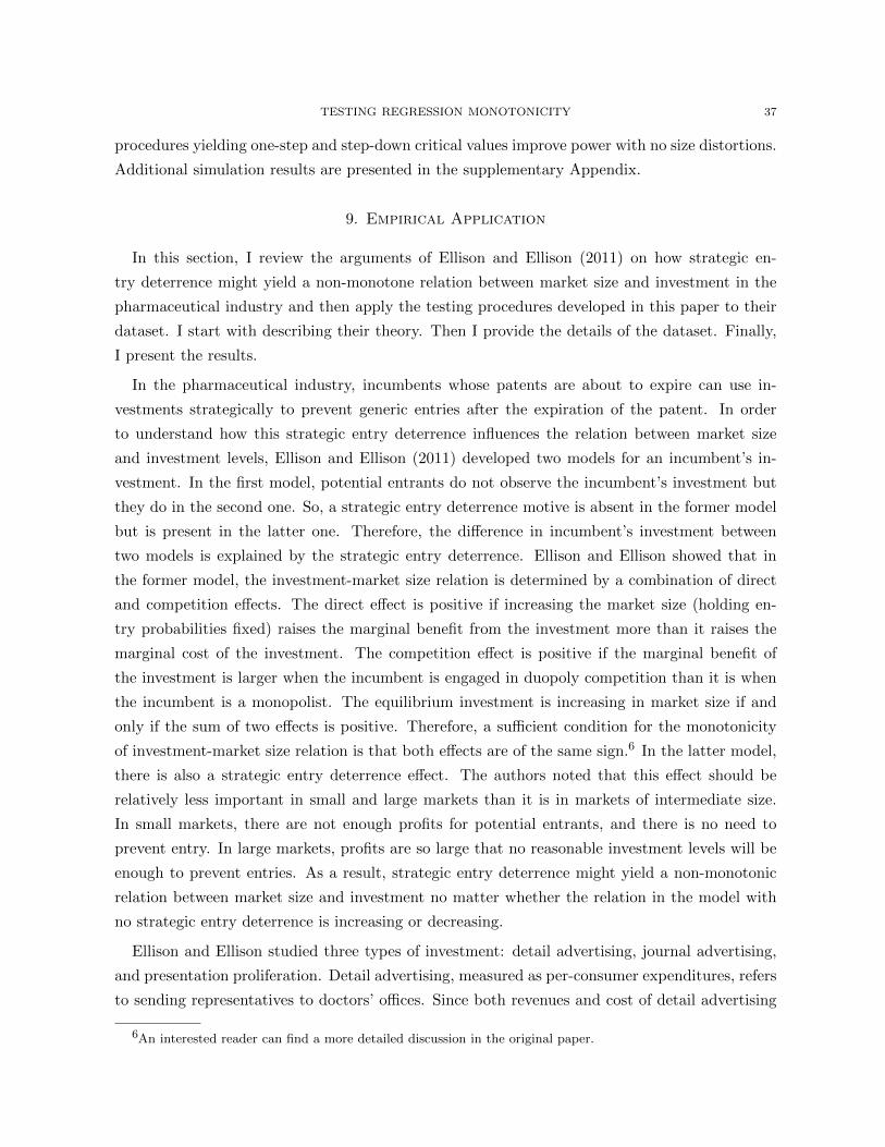
TESTING REGRESSION MONOTONICITY 37
procedures yielding one-step and step-down critical values improve power with no size distortions.
Additional simulation results are presented in the supplementary Appendix.
9. Empirical Application
In this section, I review the arguments of Ellison and Ellison (2011) on how strategic en-
try deterrence might yield a non-monotone relation between market size and investment in the
pharmaceutical industry and then apply the testing procedures developed in this paper to their
dataset. I start with describing their theory. Then I provide the details of the dataset. Finally,
I present the results.
In the pharmaceutical industry, incumbents whose patents are about to expire can use in-
vestments strategically to prevent generic entries after the expiration of the patent. In order
to understand how this strategic entry deterrence influences the relation between market size
and investment levels, Ellison and Ellison (2011) developed two models for an incumbent’s in-
vestment. In the first model, potential entrants do not observe the incumbent’s investment but
they do in the second one. So, a strategic entry deterrence motive is absent in the former model
but is present in the latter one. Therefore, the difference in incumbent’s investment between
two models is explained by the strategic entry deterrence. Ellison and Ellison showed that in
the former model, the investment-market size relation is determined by a combination of direct
and competition effects. The direct effect is positive if increasing the market size (holding en-
try probabilities fixed) raises the marginal benefit from the investment more than it raises the
marginal cost of the investment. The competition effect is positive if the marginal benefit of
the investment is larger when the incumbent is engaged in duopoly competition than it is when
the incumbent is a monopolist. The equilibrium investment is increasing in market size if and
only if the sum of two effects is positive. Therefore, a sufficient condition for the monotonicity
of investment-market size relation is that both effects are of the same sign.6 In the latter model,
there is also a strategic entry deterrence effect. The authors noted that this effect should be
relatively less important in small and large markets than it is in markets of intermediate size.
In small markets, there are not enough profits for potential entrants, and there is no need to
prevent entry. In large markets, profits are so large that no reasonable investment levels will be
enough to prevent entries. As a result, strategic entry deterrence might yield a non-monotonic
relation between market size and investment no matter whether the relation in the model with
no strategic entry deterrence is increasing or decreasing.
Ellison and Ellison studied three types of investment: detail advertising, journal advertising,
and presentation proliferation. Detail advertising, measured as per-consumer expenditures, refers
to sending representatives to doctors’ offices. Since both revenues and cost of detail advertising
6An interested reader can find a more detailed discussion in the original paper.
38 DENIS CHETVERIKOV
are likely to be linear in the market size, it can be shown that the direct effect for detail advertis-
ing is zero. The competition effect is likely to be negative because detail advertising will benefit
competitors as well. Therefore, it is expected that detail advertising is a decreasing function
of the market size in the absence of strategic distortions. Strategic entry deterrence should de-
crease detail advertising for markets of intermediate size. Journal advertising is the placement of
advertisements in medical journals. Journal advertising is also measured as per-consumer expen-
ditures. The competition effect for journal advertising is expected to be negative for the same
reason as for detail advertising. The direct effect, however, may be positive because the cost
per potential patient is probably a decreasing function of the market size. Opposite directions
of these effects make journal advertising less attractive for detecting strategic entry deterrence
in comparison with detail advertising. Nevertheless, following the original paper, I assume that
journal advertising is a decreasing function of the market size in the absence of strategic distor-
tions. Presentation proliferation is selling a drug in many different forms. Since the benefits of
introducing a new form is approximately proportional to the market size while the costs can be
regarded as fixed, the direct effect for presentation proliferation should be positive. In addition,
the competition effect is also likely to be positive because it creates a monopolistic niche for the
incumbent. Therefore, presentation proliferation should be positively related to market size in
the absence of strategic distortions.
The dataset consists of 63 chemical compounds, sold under 71 different brand names. All of
these drugs lost their patent exclusivity between 1986 and 1992. There are four variables in the
dataset: average revenue for each drug over three years before the patent expiration (this measure
should be regarded as a proxy for market size), average costs of detail and journal advertising
over the same time span as revenues, and a Herfindahl-style measure of the degree to which
revenues are concentrated in a small number of presentations (this measure should be regarded
as the inverse of presentation proliferation meaning that higher values of the measure indicate
lower presentation proliferation).
Clearly, the results will depend on how I define both dependent and independent variables
for the test. Following the strategy adopted in the original paper, I use log of revenues as
the independent variable in all cases, and the ratio of advertising costs to revenues for detail
and journal advertising and the Herfindahl-style measure for presentation proliferation as the
dependent variable. The null hypothesis is that the corresponding conditional mean function is
decreasing.7
7In the original paper, Ellison and Ellison (2011) test the null hypothesis consisting of the union of monoton-
ically increasing and monotonically decreasing regression functions. The motivation for this modification is that
increasing regression functions contradict the theory developed in the paper and, hence, should not be considered
as evidence of the existence of strategic entry deterrence. On the other hand, increasing regression functions might
TESTING REGRESSION MONOTONICITY 39
I consider the test with kernel weighting functions with k = 0 or 1 and the kernel K(x) =
0.75(1−x2) for x ∈ (−1, 1) and 0 otherwise. I use the set of bandwidth values Hn = {0.5; 1} and
the set of weighting functions Sn = {(x, h) : x ∈ {X1, ..., Xn}, h ∈ Hn}. Implementing the test
requires estimating σ2i for all i = 1, ..., n. Since the test based on Rice’s method outperformed that
with σi = εi in the Monte Carlo simulations, I use this method in the benchmark procedure. I also
check robustness of the results using the following two-step procedure. First, I obtain residuals
of the OLS regression of Y on a set of transformations of X. In particular, I use polynomials in
X up to the third degree (cubic polynomial). Second, squared residuals are projected onto the
same polynomial in X using the OLS regression again. The resulting projections are estimators
σ2i of σ2
i , i = 1, ..., n.
The results of the test are presented in table 2. The table shows the p-value of the test for
each type of investment and each method of estimating σ2i . In the table, method 1 corresponds
to estimating σ2i using Rice’s formula, and methods 2, 3, and 4 are based on polynomials of
first, second, and third degrees respectively. Note that all methods yield similar numbers, which
reassures the robustness of the results. All the methods with k = 0 reject the null hypothesis
that journal advertising is decreasing in market size with 10% confidence level. This may be
regarded as evidence that pharmaceutical companies use strategic investment in the form of
journal advertising to deter generic entries. On the other hand, recall that direct and competition
effects probably have different signs for journal advertising, and so rejecting the null may also
be due to the fact that the direct effect dominates for some values of market size. In addition,
the test with k = 1 does not reject the null hypothesis that journal advertising is decreasing in
market size at the 10% confidence level, no matter how σi are estimated. No method rejects the
null hypothesis in the case of detail advertising and presentation proliferation. This may be (1)
because firms do not use these types of investment for strategic entry deterrence, (2) because the
strategic effect is too weak to yield non-monotonicity, or (3) because the sample size is not large
enough. Overall, the results are consistent with those presented in Ellison and Ellison (2011).
10. Conclusion
In this paper, I have developed a general framework for testing monotonicity of a nonpara-
metric regression function, and have given a broad class of new tests. A general test statistic
uses many different weighting functions so that an approximately optimal weighting function is
determined automatically. In this sense, the test adapts to the properties of the model. I have
also obtained new methods to simulate the critical values for these tests. These are based on
selection procedures. The procedures are used to estimate what counterparts of the test statistic
should be used in simulating the critical value. They are constructed so that no violation of
arise if the strategic entry deterrence effect over-weighs direct and competition effects even in small and large
markets, which could be considered as extreme evidence of the existence of strategic entry deterrence.
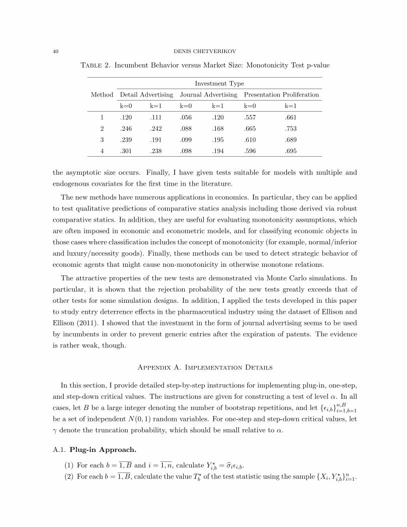
40 DENIS CHETVERIKOV
Table 2. Incumbent Behavior versus Market Size: Monotonicity Test p-value
Method
Investment Type
Detail Advertising Journal Advertising Presentation Proliferation
k=0 k=1 k=0 k=1 k=0 k=1
1 .120 .111 .056 .120 .557 .661
2 .246 .242 .088 .168 .665 .753
3 .239 .191 .099 .195 .610 .689
4 .301 .238 .098 .194 .596 .695
the asymptotic size occurs. Finally, I have given tests suitable for models with multiple and
endogenous covariates for the first time in the literature.
The new methods have numerous applications in economics. In particular, they can be applied
to test qualitative predictions of comparative statics analysis including those derived via robust
comparative statics. In addition, they are useful for evaluating monotonicity assumptions, which
are often imposed in economic and econometric models, and for classifying economic objects in
those cases where classification includes the concept of monotonicity (for example, normal/inferior
and luxury/necessity goods). Finally, these methods can be used to detect strategic behavior of
economic agents that might cause non-monotonicity in otherwise monotone relations.
The attractive properties of the new tests are demonstrated via Monte Carlo simulations. In
particular, it is shown that the rejection probability of the new tests greatly exceeds that of
other tests for some simulation designs. In addition, I applied the tests developed in this paper
to study entry deterrence effects in the pharmaceutical industry using the dataset of Ellison and
Ellison (2011). I showed that the investment in the form of journal advertising seems to be used
by incumbents in order to prevent generic entries after the expiration of patents. The evidence
is rather weak, though.
Appendix A. Implementation Details
In this section, I provide detailed step-by-step instructions for implementing plug-in, one-step,
and step-down critical values. The instructions are given for constructing a test of level α. In all
cases, let B be a large integer denoting the number of bootstrap repetitions, and let {εi,b}n,Bi=1,b=1
be a set of independent N(0, 1) random variables. For one-step and step-down critical values, let
γ denote the truncation probability, which should be small relative to α.
A.1. Plug-in Approach.
(1) For each b = 1, B and i = 1, n, calculate Y ?i,b = σiεi,b.
(2) For each b = 1, B, calculate the value T ?b of the test statistic using the sample {Xi, Y?i,b}ni=1.
TESTING REGRESSION MONOTONICITY 41
(3) Define the plug-in critical value, cPI1−α, as the (1− α) sample quantile of {T ?b }Bb=1.
A.2. One-Step Approach.
(1) For each b = 1, B and i = 1, n, calculate Y ?i,b = σiεi,b.
(2) Using the plug-in approach, simulate cPI1−γ .
(3) Define SOSn as the set of values s ∈ Sn such that b(s)/(V (s))1/2 > −2cPI1−γ .
(4) For each b = 1, B, calculate the value T ?b of the test statistic using the sample {Xi, Y?i,b}ni=1
and taking maximum only over SOSn instead of Sn.
(5) Define the one-step critical value, cOS1−α, as the (1− α) sample quantile of {T ?b }Bb=1.
A.3. Step-down Approach.
(1) For each b = 1, B and i = 1, n, calculate Y ?i,b = σiεi,b.
(2) Using the plug-in and one-step approaches, simulate cPI1−γ and cOS1−γ , respectively.
(3) Denote S1n = SOSn , c1 = cOS1−γ , and set l = 1.
(4) For given value of l > 1, define S l+1n as the set of values s ∈ S ln such that b(s)/(V (s))1/2 >
−cPI1−γ − cl.(5) For each b = 1, B, calculate the value T ?b of the test statistic using the sample {Xi, Y
?i,b}ni=1
and taking the maximum only over S l+1n instead of Sn.
(6) Define cl+1, as the (1− γ) sample quantile of {T ?b }Bb=1.
(7) If S l+1n = S ln, then go to step (8). Otherwise, set l = l + 1 and go to step (4).
(8) For each b = 1, B, calculate the value T ?b of the test statistic using the sample {Xi, Y?i,b}ni=1
and taking the maximum only over S ln instead of Sn.
(9) Define cSD1−α, as the (1− α) sample quantile of {T ?b }Bb=1.
Appendix B. Verification of High-Level Conditions
This section verifies high level assumptions used in Section 4 under primitive conditions. As-
sumptions used in Sections 5, 6, and 7 can be verified by similar arguments. First, I consider
Assumption A3, which concerns the uniform consistency of the estimator σi of σi over i = 1, n.
Second, I verify Assumption A4 and derive a bound on the sensitivity parameter An when ker-
nel weighting functions are used. This allows me to verify Assumption A5. Finally, I provide
primitive conditions for Assumption A9.
Let C6 and L′ be strictly positive constants. The following proposition proves consistency of
the local version of Rice’s estimator.
Proposition B.1 (Verifying Assumption A3). Suppose that σi is the local version of Rice’s
estimator of σi given in equation (12). Suppose also that (i) Assumptions A1 and A8 hold, (ii)
bn > (log n)2/(C6n), (iii) |f(Xi)− f(Xj)| 6 L′|Xi −Xj | for all i, j = 1, n, and (iv) |σ2i − σ2
j | 6
42 DENIS CHETVERIKOV
L′|Xi − Xj | for all i, j = 1, n. Then max16i6n |σi − σi| = Op(b2n + log n/(bnn
1/2)), and so
Assumption A3 holds with any κ2 satisfying b2n + log n/(bnn1/2) = o(n−κ2).
Next, I consider restrictions on the weighting functions to ensure that Assumption A4 holds
and give an upper bound on the sensitivity parameter An.
Proposition B.2 (Verifying Assumptions A4 and A5). Suppose that kernel weighting functions
are used. In addition, suppose that (i) Assumptions A1 and A8 hold, (ii) K(·) has the support
[−1,+1], is continuous, and strictly positive on the interior of its support, (iii) x ∈ [sl, sr]
for all (x, h) ∈ Sn, (iv) hmin > (log n)2/(C6n) w.p.a.1 where hmin = min(x,h)∈Sn h, and (v)
hmax 6 (sr − sl)/2 where hmax = max(x,h)∈Sn h. Then (a) An 6 C/(nhmin)1/2 w.p.a.1 for some
C > 0, and so Assumption A5 holds for the basic set of weighting functions; (b) if Assumption
A3 is satisfied, then Assumption A4 holds with κ3 = κ2; (c) if Assumption A2 is satisfied, then
Assumption A4 holds with κ3 = κ1 as long as log p/(hminn1/2) = op(n
−κ1).
Restrictions on the kernel K(·) imposed in this lemma are satisfied for most commonly used
kernel functions including uniform, triangular, Epanechnikov, biweight, triweight, and tricube
kernels. Note, however, that these restrictions exclude higher order kernels since those are neces-
sarily negative at some points on their supports. Assumption A8 imposes the restriction that the
density of X is bounded below from zero on its support. This is needed to make sure that V (s)
is sufficiently well separated from zero since V (s) appears in the denominator of the test statistic
T . Alternatively, one can truncate V (s) from below with the truncation parameter converging
to zero with an appropriate rate as the sample size n increases. I do not consider this possibility
for brevity of the paper. Finally, I verify Assumption A9.
Proposition B.3 (Verifying Assumption A9). Suppose that the basic set of weighting functions
is used. In addition, suppose that (i) Assumption A8 holds and (ii) K(·) has the support [−1,+1],
is continuous, and strictly positive on the interior of its support. Then Assumption A9 holds.
Appendix C. Additional Notation
I will use the following additional notation in Appendices C and D. Recall that {εi} is a
sequence of independent N(0, 1) random variables that are independent of the data. Denote
ei = σiεi and ei = σiεi for i = 1, n. Let
wi(s) =∑
16j6n
sign(Xj −Xi)Q(Xi, Xj , s),
ai(s) = wi(s)/(V (s))1/2 and ai(s) = wi(s)/(V (s))1/2,
e(s) =∑
16i6n
ai(s)ei, and e(s) =∑
16i6n
ai(s)ei,
TESTING REGRESSION MONOTONICITY 43
ε(s) =∑
16i6n
ai(s)εi and ε(s) =∑
16i6n
ai(s)εi,
f(s) =∑
16i6n
ai(s)f(Xi) and f(s) =∑
16i6n
ai(s)f(Xi).
Note that T = maxs∈Sn∑
16i6n ai(s)Yi = maxs∈Sn(f(s) + ε(s)). In addition, for any S ⊂ Sn,
which may depend on {Xi}16i6n, and all η ∈ (0, 1), let cSη denote the conditional η quantile of
T ? = T ({Xi, Y?i }, {σi},S) given {Xi}, {σi}, and S where Y ?
i = σiεi for i = 1, n, and let cS,0η
denote the conditional η quantile of T ? = T ({Xi, Y?i }, {σi},S) given {Xi} and S where Y ?
i = σiεi
for i = 1, n. Further, for η 6 0, define cSη and cS,0η as −∞, and for η > 1, define cSη and cS,0η as
+∞.
In the next section, I prove some auxiliary lemmas. For these lemmas, it will be convenient
to use the following additional notation. Recall that Sn is a set that is allowed to depend on
{Xi}. In addition, I will need some subsets of Sn that are selected from Sn according to certain
mappings that also depend {Xi}, i.e. S = S(Sn, {Xi}) ⊂ Sn. Some results will be stated to hold
uniformly over all mappings S(·, ·).
Let {ψn} be a sequence of positive numbers converging to zero sufficiently slowly so that (i)
log p/nκ3 = op(ψn) (recall that by Assumption A5, log p/nκ3 = op(1), and so such a sequence
exists), (ii) uniformly over all S(·, ·) and η ∈ (0, 1), P(cS,0η+ψn< cSη ) = o(1) and P(cSη+ψn
<
cS,0η ) = o(1) where S = S(Sn, {Xi}) (Lemma D.5 establishes existence of such a sequence under
Assumptions A1, A3, A4, and A5 and Lemma D.7 establishes existence under Assumptions A1,
A2, A4, and A5). Let
SRn = {s ∈ Sn : f(s) > −cSn,01−γn−ψn}.
For D = PI,OS, SD,R, let cDη = cSDnη and cD,0η = c
SDn ,0η where SPIn = Sn. Note that cPI,0η and
cR,0η are non-stochastic.
Moreover, I denote V = maxs∈Sn(V (s)/V (s))1/2. Finally, I denote the space of k-times con-
tinuously differentiable functions on R by Ck(R,R). For g ∈ Ck(R,R), the symbol g(r) for r 6 k
denotes the rth derivative of g, and ‖g(r)‖∞ = supt∈R |g(r)(t)|.
Appendix D. Proofs for section 4
In this Appendix, I first prove a sequence of auxiliary lemmas (Subsection D.1). Then I present
the proofs of the theorems stated in Section 4 (Subsection D.2). In Subsection D.1, all results
hold uniformly over all models M ∈ M. For simplicity of notation, however, I drop index M
everywhere.
D.1. Auxiliary Lemmas.
Lemma D.1. E[maxs∈Sn |e(s)||{Xi}] 6 C(log p)1/2 for some universal C > 0.

44 DENIS CHETVERIKOV
Proof. Note that by construction, conditional on {Xi}, e(s) is distributed as a N(0, 1) random
variable, and |Sn| = p. So, the result follows from lemma 2.2.2 in Van der Vaart and Wellner
(1996). �
Lemma D.2. For all S(·, ·) and ∆ > 0,
supt∈R
P
(maxs∈S
e(s) ∈ [t, t+ ∆]|{Xi})6 C∆(log p)1/2
and for all S(·, ·) and (η, δ) ∈ (0, 1)2,
cS,0η+δ − cS,0η > Cδ/(log p)1/2
for some universal C > 0 where S = S(Sn, {Xi}).
Proof. Theorem 3 in Chernozhukov, Chetverikov, and Kato (2011) shows that if W1, . . . ,Wp is
a sequence of N(0, 1) random (not necessarily independent) variables, then for all ∆ > 0,
supt∈R
P
(max16j6p
Wj ∈ [t, t+ ∆]
)6 4∆
(E
[max16j6p
Wj
]+ 1
).
Therefore,
supt∈R
P
(maxs∈S
e(s) ∈ [t, t+ ∆]|{Xi})6 4∆
(E
[maxs∈S
e(s)|{Xi}]
+ 1
),
and so the first claim follows from Lemma D.1. The second claim follows from the result in the
first claim. �
Lemma D.3. For all S(·, ·), η ∈ (0, 1), and t ∈ R,
cS,0η−C|t| log p/(1−η) 6 cS,0η (1 + t) 6 cS,0η+C|t| log p/(1−η)
for some universal C > 0 where S = S(Sn, {Xi}).
Proof. Recall that cS,0η is the conditional η quantile of maxs∈S e(s) given {Xi}, and so combining
Lemma D.1 and Markov inequality shows that cS,0η 6 C(log p)1/2/(1 − η) for some universal
C > 0. Therefore, Lemma D.2 gives
cS,0η+C|t| log p/(1−η) − cS,0η > C|t|(log p)1/2/(1− η) > |t|cS,0η (33)
if C > 0 is sufficiently large in (33). The lower bound follows similarly. �
Lemma D.4. Under Assumptions A1 and A5, uniformly over all S(·, ·) and η ∈ (0, 1),
P
(maxs∈S
ε(s) 6 cS,0η
)= η + o(1) and P
(maxs∈S
(−ε(s)) 6 cS,0η
)= η + o(1)
where S = S(Sn, {Xi}).
TESTING REGRESSION MONOTONICITY 45
Proof. Note that∑
16i6n(ai(s)σi)2 = 1. In addition, by Assumption A5, nA4
n(log(pn))7 = op(1),
and so there exists a sequence {ωn} of positive numbers such that nA4n(log(pn))7 = op(ωn) and
ωn = o(1). Let An denote the event that nA4n(log(pn))7 > ωn. Then P(An) = o(1). Further, note
that E[ε2i /σ
2i |Xi] = 1, and since E[ε4
i |Xi] 6 C1 and σi > c1 by Assumption A1, E[ε4i /σ
4i |Xi] 6 C
for some C > 0. Therefore, applying Lemma H.4, case (ii), with zis =√nai(s)σi and ui = εi/σi
conditional on {Xi} shows that there exists a sequence {ω′} of positive numbers converging to
zero and depending only on {ωn} such that outside of An,∣∣∣∣P(maxs∈S
ε(s) 6 cS,0η |{Xi})− η∣∣∣∣ 6 ω′n.
Since P(An) = o(1), this implies that
P
(maxs∈S
ε(s) 6 cS,0η
)= η + o(1),
which gives the first asserted claim. The second claim follows by replacing ε(s) by −ε(s). Note
that since the sequence {ω′n} depends only on the sequence {ωn}, it follows that the result of
this lemma holds uniformly over all models M ∈M. �
Lemma D.5. Under Assumptions A1, A3, A4, and A5, there exists a sequence {ψn} of positive
numbers converging to zero such that uniformly over all S(·, ·) and η ∈ (0, 1), P(cS,0η+ψn< cSη ) =
o(1) and P(cSη+ψn< cS,0η ) = o(1) where S = S(Sn, {Xi}).
Proof. Denote
TS = maxs∈S
e(s) = maxs∈S
∑16i6n
ai(s)σiεi and TS,0 = maxs∈S
e(s) = maxs∈S
∑16i6n
ai(s)σiεi.
In addition, denote
p1 = maxs∈S|e(s)|max
s∈S
∣∣∣1− (V (s)/V (s))1/2∣∣∣ ,
p2 = maxs∈S
∣∣∣∣∣ ∑16i6n
ai(s)(σi − σi)εi
∣∣∣∣∣maxs∈S
(V (s)/V (s))1/2.
Then |TS − TS,0| 6 p1 + p2. Combining Lemma D.1 and Assumption A4 gives
p1 = op
((log p)1/2n−κ3
).
Consider p2. Conditional on {σi}, (σi − σi)εi is distributed as a N(0, (σi − σi)2) random vari-
able, and so applying the argument like that in Lemma D.1 conditional on {Xi, σi} and using
Assumption A3 gives
maxs∈S
∣∣∣∣∣ ∑16i6n
ai(s)(σi − σi)εi
∣∣∣∣∣ = op
((log p)1/2n−κ2
).
Since maxs∈S(V (s)/V (s))1/2 →p 1 by Assumption A4, this implies that
p2 = op
((log p)1/2n−κ2
).

46 DENIS CHETVERIKOV
Therefore, TS − TS,0 = op((log p)1/2n−κ2∧κ3), and so there exists a sequence {ψn} of positive
numbers converging to zero such that
P(|TS − TS,0| > (log p)1/2n−κ2∧κ3
)= o(ψn).
Hence,
P(
P(|TS − TS,0| > (log p)1/2n−κ2∧κ3 |{Xi, σi}
)> ψn
)→ 0.
Let An denote the event that
P(|TS − TS,0| > (log p)1/2n−κ2∧κ3 |{Xi, σi}
)6 ψn.
I will take ψn = ψn +C(log p)n−κ2∧κ3 for a constant C that is larger than that in the statement
of Lemma D.2. By assumption A5, ψn → 0. Then note that
P(TS,0 6 cS,0η |{Xi, σi}
)> η and P
(TS 6 cSη |{Xi, σi}
)> η
for any η ∈ (0, 1). So, on An,
η + ψn 6 P(TS,0 6 cS,0
η+ψn|{Xi, σi}
)6 P
(TS 6 cS,0
η+ψn+ (log p)1/2n−κ2∧κ3 |{Xi, σi}
)+ ψn 6 P
(TS 6 cS,0η+ψn
|{Xi, σi})
+ ψn
where the last inequality follows from Lemma D.2. Therefore, on An, cSη 6 cS,0η+ψn
, i.e. P(cS,0η+ψn<
cSη ) = o(1). The second claim follows similarly. �
Lemma D.6. Let cS,1η denote the conditional η quantile of TS,1 = maxs∈S∑
16i6n ai(s)εiεi given
{Xi, εi}. Let Assumptions A1, A2, and A5 hold. Then there exists a sequence {ψn} of positive
numbers converging to zero such that uniformly over all S(·, ·) and η ∈ (0, 1), P(cS,0η+ψn
< cS,1η ) =
o(1) and P(cS,1η+ψn
< cS,0η ) = o(1) where S = S(Sn, {Xi}).
Proof. Let Z1 = {∑
16i6n ai(s)εiεi}s∈S and Z2 = {∑
16i6n ai(s)σiεi}s∈S . Conditional on {Xi, εi},these are zero-mean Gaussian vectors in R|S| with covariances Σ1 and Σ2 given by
Σ1s1s2 =
∑16i6n
ai(s1)ai(s2)ε2i and Σ2
s1s2 =∑
16i6n
ai(s1)ai(s2)σ2i .
Let ∆Σ = maxs1,s2∈S |Σ1s1s2 − Σ2
s1s2 |. Applying Lemma H.2 shows that under Assumption A1,
for some C > 0,
E [∆Σ|{Xi}] 6 C
(An√
log p+A2n log pE
[max16i6n
ε4i |{Xi}
]1/2).
Further, E[max16i6n ε4i |{Xi}] 6
∑16i6n E[ε4
i |{Xi}] 6 Cn for some C > 0 by Assumption A1,
and so Assumption A5 implies that
(log p)2∆Σ = op(1) (34)
TESTING REGRESSION MONOTONICITY 47
because A2n(log p)3n1/2 = op(1) and An(log p)5/2 = op(1) (to verify the latter equation, recall
that log p/n1/4 = o(1) by Assumption A5; taking square of this equation and multiplying it
by A2n(log p)3n1/2 = op(1) gives An(log p)5/2 = op(1)). Therefore, it follows that there exists a
sequence {ψn} of positive numbers converging to zero such that
(log p)2∆Σ = op(ψ4n). (35)
Let g ∈ C2(R,R) be a function satisfying g(t) = 1 for t 6 0, g(t) = 0 for t > 1, and g(t) ∈ [0, 1]
for t ∈ [0, 1], and let gn(t) = g((t− cS,0η+ψn/2
)/(cS,0η+ψn
− cS,0η+ψn/2
)). Then for some C > 0, Lemma
D.2 shows that
‖g(1)n ‖∞ 6 ‖g(1)‖∞/
(cS,0η+ψn
− cS,0η+ψn/2
)6 C(log p)1/2/ψn,
‖g(2)n ‖∞ 6 ‖g(2)‖∞/
(cS,0η+ψn
− cS,0η+ψn/2
)26 C(log p)/ψ2
n.
Applying Lemma H.3 gives for some C > 0,
Dn =
∣∣∣∣E [gn(maxs∈S
Z1s
)− gn
(maxs∈S
Z2s
)|{Xi, εn}
]∣∣∣∣ (36)
6 C(
(log p)∆Σ/ψ2n + (log p)(∆Σ)1/2/ψn
)= op(ψn) (37)
by equation (35). Note that maxs∈S Z1s = TS,1 and, using the notation in the proof of Lemma
D.5, maxs∈S Z2s = TS,0. Therefore,
P(TS,1 6 cS,0
η+ψn|{Xi, εi}
)>(1) E
[gn(TS,1)|{Xi, εi}
]>(2) E
[gn(TS,0)|{Xi, εi}
]−Dn
>(3) P(TS,0 6 cS,0
η+ψn/2|{Xi, εi}
)−Dn
=(4) P(TS,0 6 cS,0
η+ψn/2|{Xi}
)−Dn > η + ψn/2−Dn (38)
where (1) and (3) are by construction of the function gn, (2) is by the definition of Dn, and (4)
is because TS,0 and cS,0η+ψn/2
are jointly independent of {εi}. Finally, note that the right hand
side of line (38) is bounded from below by η w.p.a.1. This implies that P(cS,0η+ψn
< cS,1η ) = o(1),
which is the first asserted claim. The second claim of the lemma follows similarly. �
Lemma D.7. Under Assumptions A1, A2, A4, and A5, there exists a sequence {ψn} of positive
numbers converging to zero such that uniformly over all S(·, ·) and η ∈ (0, 1), P(cS,0η+ψn< cSη ) =
o(1) and P(cSη+ψn< cS,0η ) = o(1) where S = S(Sn, {Xi}).8
Proof. Lemma D.6 established that
P(cS,0η+ψn
< cS,1η ) = o(1) and P(cS,1η+ψn
< cS,0η ) = o(1).
8Note that Lemmas D.5 and D.7 provide the same results under two different methods for estimating σi.
48 DENIS CHETVERIKOV
Therefore, it suffices to show that
P(cSη+ψn
< cS,1η ) and P(cS,1η+ψn
< cSη )
for some sequence {ψn} of positive numbers converging to zero. Denote
p1 = maxs∈S
∣∣∣∣∣ ∑16i6n
ai(s)εiεi
∣∣∣∣∣maxs∈S
∣∣∣1− (V (s)/V (s))1/2∣∣∣ ,
p2 = maxs∈S
∣∣∣∣∣ ∑16i6n
ai(s)(σi − εi)εi
∣∣∣∣∣maxs∈S
(V (s)/V (s))1/2.
Note that |TS − TS,1| 6 p1 + p2 and that by Lemmas D.1 and D.6, maxs∈S |∑
16i6n ai(s)εiεi| =Op((log p)1/2). Therefore, the result follows by the argument similar to that used in the proof of
Lemma D.5 since σi − εi = op(n−κ1) by Assumption A2. �
Lemma D.8. Let Assumptions A1, A4, and A5 hold. In addition, let either Assumption A2 or
A3 hold. Then P(SRn ⊂ SSDn ) > 1− γn + o(1) and P(SRn ⊂ SOSn ) > 1− γn + o(1).
Proof. By the definition of ψn, log p/nκ3 = op(ψn), and so there exists a sequence {ωn} of
positive numbers converging to zero such that log p/nκ3 = op(ωnψn). Let An denote the event
that log p/nκ3 > ωnψn. Then P(An) = o(1).
Further, suppose that SRn \SSDn 6= ∅. Then there exists the smallest integer l such that SRn \S ln 6=∅ and SRn ⊂ S l−1
n (if l = 1, let S0n = Sn). Therefore, cR1−γn 6 cl−1
1−γn . It follows that there exists
an element s of SRn such that
f(s) + ε(s) 6 −cPI1−γn − cl−11−γn 6 −c
PI1−γn − c
R1−γn ,
and so for some C > 0,
P(SRn \SSDn 6= ∅) 6 P( mins∈SRn
(f(s) + ε(s)) 6 −cPI1−γn − cR1−γn)
6(1) P(( mins∈SRn
(f(s) + ε(s))V 6 −cPI1−γn − cR1−γn)
6(2) P(( mins∈SRn
(f(s) + ε(s))V 6 −cPI,01−γn−ψn − cR,01−γn−ψn) + o(1)
6(3) P(( mins∈SRn
(ε(s)− cPI,01−γn−ψn)V 6 −cPI,01−γn−ψn − cR,01−γn−ψn) + o(1)
=(4) P((maxs∈SRn
(−ε(s)) > cPI,01−γn−ψn(1/V − 1) + cR,01−γn−ψn/V) + o(1)
6(5) P((maxs∈SRn
(−ε(s)) > cR,01−γn−ψn/V − C(log p)1/2n−κ3/(γn + ψn)) + o(1)
6(6) P((maxs∈SRn
(−ε(s)) > cR,01−γn−ψn−C(log p)n−κ3/(γn+ψn)
) + o(1)
6(7) γn + ψn + Cωn + P(An) + o(1) =(8) γn + o(1)

TESTING REGRESSION MONOTONICITY 49
where (1) follows from the definitions of f(s) and ε(s), (2) is by the definition of ψn, (3) is by
the definition of SRn , (4) is rearrangement, (5) is by Lemma D.1 and Assumption A4, (6) is by
Lemmas D.2 and D.3, (7) is by Lemma D.4 and definitions of ωn and An, and (8) follows from
the definition of ψn again. The first asserted claim follows. The second claim follows from the
fact that SSDn ⊂ SOSn . �
Lemma D.9. Let Assumptions A1, A4, and A5 hold. In addition, let either Assumption A2 or
A3 hold. Then P(maxs∈Sn\SRn (f(s) + ε(s)) 6 0) > 1− γn + o(1).
Proof. The result follows from
P( maxs∈Sn\SRn
(f(s) + ε(s)) 6 0) = P( maxs∈Sn\SRn
(f(s) + ε(s)) 6 0)
>(1) P( maxs∈Sn\SRn
ε(s) 6 cPI,01−γn−ψn)
> P(maxs∈Sn
ε(s) 6 cPI,01−γn−ψn)
=(2) 1− γn − ψn + o(1) =(3) 1− γn + o(1)
where (1) follows from the definition of SRn , (2) is by Lemma D.4, and (3) is by the definition of
ψn. �
D.2. Proofs of Theorems.
Proof of Theorem 4.1. All inequalities presented in this proof hold uniformly over all models
M ∈M because all of them only rely on assumptions and lemmas in Subsection D.1, which hold
uniformly over all models M ∈M. For brevity of notation, I drop indexing by M .
By the definition of ψn, log p/nκ3 = op(ψn), and so there exists a sequence {ωn} of positive
numbers converging to zero such that log p/nκ3 = op(ωnψn). Let An denote the event that
log p/nκ3 > ωnψn. Then P(An) = o(1).
Further, note that for some C > 0,
P(T 6 cP1−α) = P(maxs∈Sn
(f(s) + ε(s)) 6 cP1−α) >(1) P(maxs∈SRn
(f(s) + ε(s)) 6 cP1−α)− γn + o(1)
>(2) P(maxs∈SRn
(f(s) + ε(s)) 6 cR1−α)− 2γn + o(1) >(3) P(maxs∈SRn
ε(s) 6 cR1−α)− 2γn + o(1)
>(4) P(maxs∈SRn
ε(s)V 6 cR,01−α−ψn)− 2γn + o(1) =(5) P(maxs∈SRn
ε(s) 6 cR,01−α−ψn/V)− 2γn + o(1)
>(6) P(maxs∈SRn
ε(s) 6 cR,01−α−ψn(1− n−κ3))− 2γn + o(1)
>(7) P(maxs∈SRn
ε(s) 6 cR,01−α−ψn−C(log p)n−κ3/(α+ψn)
)− 2γn + o(1)
>(8) 1− α− ψn − Cωn − P(An)− 2γn + o(1) =(9) 1− α+ o(1)

50 DENIS CHETVERIKOV
where (1) follows from Lemma D.9, (2) is by Lemma D.8, (3) is because under H0, f(s) 6 0, (4)
follows from the definitions of ε(s) and ψn, (5) is rearrangement, (6) is by Assumption A4, (7) is
by Lemma D.3, (8) is by Lemma D.4 and definitions of ωn and An, and (9) is by the definitions
of ψn and γn. The first asserted claim follows.
In addition, when f(·) is identically constant,
P(T 6 cP1−α) =(1) P(maxs∈Sn
ε(s) 6 cP1−α) 6(2) P(maxs∈Sn
ε(s) 6 cPI1−α)
6(3) P(maxs∈Sn
ε(s) 6 cPI,01−α+ψn) + o(1) 6(4) P(max
s∈Snε(s) 6 cPI,01−α+ψn
(1 + n−κ3)) + o(1)
6(5) P(maxs∈Sn
ε(s) 6 cPI,01−α+ψn+C(log p)n−κ3/(α−ψn)
) + o(1) 6(6) 1− α+ o(1)
where (1) follows from the fact that f(s) = 0 whenever f(·) is identically constant, (2) follows
from SPn ⊂ Sn, (3) is by the definition of ψn, (4) is by Assumption A4, (5) is by Lemma D.3, and
(6) is from Lemma D.4 and the definition of ψn. The second asserted claim follows. �
Proof of Theorem 4.2. Let x1, x2 ∈ [sl, sr] be such that x1 < x2 but f(x1) > f(x2). By the mean
value theorem, there exists x0 ∈ (x1, x2) satisfying
f ′(x0)(x2 − x1) = f(x2)− f(x1) < 0.
Therefore, f ′(x0) < 0. Since f ′(·) is continuous, f ′(x) < f ′(x0)/2 for any x ∈ [x0 −∆x, x0 + ∆x]
for some ∆x > 0. Apply Assumption A7 to the interval [x0−∆x, x0 + ∆x] to obtain s = sn ∈ Snand intervals [xl1, xr1] and [xl2, xr2] appearing in Assumption A7-iii. By Assumption A7-ii,
V (s) 6 Cn3 (39)
for some C > 0. In addition, by Assumption A6 and Chebyshev’s inequality, there is some C > 0
such that |{i = 1, n : Xi ∈ [xl1, xr1]}| > Cn and |{i = 1, n : Xi ∈ [xl2, xr2]}| > Cn w.p.a.1.
Hence, by Assumptions A7-(i) and A7-(iii),∑16i,j6n
(f(Xi)− f(Xj))sign(Xj −Xi)Q(Xi, Xj , s) > Cn2 (40)
w.p.a.1 for some C > 0. Combining (39) and (40) yields f(s) > Cn1/2 w.p.a.1 for some C > 0. Let
An denote the event that f(s) < Cn1/2, so that P(An) = o(1). Further, since∑
16i6n ai(s)2σ2i =
1, Assumption A1 implies An > C/n1/2 for some C > 0, and so Assumption A5 gives log p =
op(n), and so
(log p)1/2 = op(f(s)). (41)
Therefore, there exists a sequence {ωn} of positive numbers converging to zero such that (log p)1/2 =
op(ωnf(s)), and so letting Bn denote the event that (log p)1/2 > ωnf(s) leads to P(Bn) = o(1).
TESTING REGRESSION MONOTONICITY 51
Hence, for some C > 0,
P(T 6 cP1−α) 6(1) P(T 6 cPI1−α) 6(2) P(T 6 cPI,01−α+ψn) + o(1)
6(3) P(T 6 C(log p)1/2) + o(1) 6(4) P(f(s) + ε(s) 6 C(log p)1/2) + o(1)
6(5) P(f(s) + ε(s) 6 C(log p)1/2(1 + n−κ3)) + o(1)
6(6) P(f(s) + ε(s) 6 2C(log p)1/2) + o(1)
6(7) P(ε(s) 6 2C(log p)1/2 − f(s)) + o(1)
6(8) P(ε(s) 6 (2Cωn − 1)f(s)) + P(Bn) + o(1)
6(9) C/n+ P(An) + P(Bn) + o(1) =(10) o(1)
where (1) follows from SPn ⊂ SPIn , (2) is by the definition of ψn, (3) is by Lemma D.1, (4) is since
T = maxs∈Sn(f(s) + ε(s)), (5) is by Assumption A4, (6) is because n−κ3 6 1 for large n, (7) is
rearrangement, (8) follows from definitions of ωn and Bn, (9) follows by noting that 2Cωn 6 1/2
for large n and applying Chebyshev’s inequality conditional on {Xi} with E[ε(s)2|{Xi}] = 1, and
(10) follows from P(An) + P(Bn) = o(1). This completes the proof of the theorem. �
Proof of Theorem 4.3. The proof follows from an argument similar to that used in the proof of
Theorem 4.2 with equation (40) replaced by∑16i,j6n
(f(Xi)− f(Xj))sign(Xj −Xi)Q(Xi, Xj , s) > Clnn2,
so that f(s) > Clnn1/2 w.p.a.1 for some C > 0, and condition log p = op(n) replaced by log p =
op(l2nn), so that (log p)1/2 = op(f(s)). �
Proof of Theorem 4.4. Since infx∈[sl,sr] f(1)(x) < −ln(log p/n)β/(2β+3), for sufficiently large n,
there exists an interval [xn,1, xn,2] ⊂ [sl, sr] such that |xn,2−xn,1| = hn and for all x ∈ [xn,1, xn,2],
f (1)(x) < −ln(log p/n)β/(2β+3)/2. Take s = sn ∈ Sn as in Assumption A9 applied to the interval
[xn,1, xn,2]. Assumptions A1, A8, and A9-(ii) yield V (s) 6 C(nhn)3h2kn for some C > 0 because by
Lemma H.1, |{i = 1, n : Xi ∈ [xn,1, xn,2]}| 6 Cnhn w.p.a.1. In addition, combining Assumptions
A8, A9-(i), and A9-(iii),∑16i,j6n
(f(Xi)− f(Xj))sign(Xj −Xi)Q(Xi, Xj , s) > lnCh1+β+kn (nhn)2
w.p.a.1 for some C > 0, and so f(s) > Clnh1+βn (nhn)1/2 w.p.a.1 by an argument similar to that
used in the proof of Theorem 4.2. From this point, since log p = o(l2nh2β+3n n), the argument like
that used in the proof of Theorem 4.2 yields the result. �
Proof of Theorem 4.5. Let sl = 0 and sr = 1. Let h = hn = c(log n/n)1/(2β+3) for sufficiently
small c > 0. Let L = [(sr − sl)/(4h)] where [x] is the largest integer smaller or equal than x.
For l = 1, L, let xl = 4h(l − 1) and define fl : [sl, sr] → R by fl(sl) = 0, f(1)l (x) = 0 if x 6 xl,
52 DENIS CHETVERIKOV
f(1)l (x) = −L(x − xl)β if x ∈ (xl, xl + h], f
(1)l (x) = −L(xl + 2h − x)β if x ∈ (xl + h, xl + 2h],
f(1)l (x) = L(x−xl−2h)β if x ∈ (xl+2h, xl+3h], f
(1)l (x) = L(xl+4h−x)β if x ∈ (xl+3h, xl+4h]
and f(1)l (x) = 0 otherwise. In addition, let f0(x) = 0 for all x ∈ [sl, sr]. Finally, let {εi} be a
sequence of independent N(0, 1) random variables.
For l = 0, L, consider a model Ml = Mn,l with the regression function fl, X distributed
uniformly over [0, 1], and ε distributed as N(0, 1) random variable independently of X. Note
that M0 belongs to M2 and satisfies H0. In addition, for l > 1, Ml belongs to M2, does not
satisfy H0, and, moreover, has infx∈[sl,sr] f(1)l (x) < −C(log n/n)β/(2β+3) for some small C > 0.
Consider any test ψ = ψ({Xi, Yi}) such that EM0 [ψ] 6 α+ o(1). Then following the argument
from Dumbgen and Spokoiny (2001) gives
infM∈M2
EM [ψ]− α 6 min16l6L
EMl[ψ]− EM0 [ψ] + o(1) 6
∑16l6L
EMl[ψ]/L− EM0 [ψ] + o(1)
=∑
16l6L
EM0 [ψρl]/L− EM0 [ψ] + o(1) =∑
16l6L
EM0 [ψ(ρl − 1)]/L+ o(1)
6 EM0
ψ∣∣∣∣∣∣∑
16l6L
ρl/L− 1
∣∣∣∣∣∣+ o(1) 6 EM0
∣∣∣∣∣∣∑
16l6L
ρl/L− 1
∣∣∣∣∣∣+ o(1)
where ρl is the likelihood ratio of observing {Xi, Yi} under the models Ml and M0. Further,
ρl = exp
( ∑16i6n
Yifl(Xi)−∑
16i6n
fl(Xi)2/2
)= exp(ωn,lξn,l − ω2
n,l/2)
where ωn,l = (∑
16i6n fl(Xi)2)1/2 and ξn,l =
∑16i6n Yifl(Xi)/ωn,l. Note that under the model
M0, conditional on {Xi}, {ξn,l}16l6L is a sequence of independent N(0, 1) random variables, so
that
EM0
∣∣∣∣∣∣∑
16l6L
ρl/L− 1
∣∣∣∣∣∣ |{Xi}
6 2.
In addition, by the construction of the functions fl, Lemma H.1 shows that ωn,l 6 C(nh)1/2hβ+1
w.p.a.1 for some C > 0, and so ωn,l 6 (C log n)1/2 w.p.a.1 for some C > 0 where C can be made
arbitrarily small by selecting sufficiently small c in the definition of hn. Let An denote the event
ωn,l 6 (C log n)1/2, so that P(An)→ 1. Moreover,
EM0
∣∣∣∣∣∣∑
16l6L
ρl/L− 1
∣∣∣∣∣∣ 6 EM0
∣∣∣∣∣∣∑
16l6L
ρl/L− 1
∣∣∣∣∣∣ |An+ 2(1− P(An)). (42)

TESTING REGRESSION MONOTONICITY 53
Further, on An,
EM0
∣∣∣∣∣∣∑
16l6L
ρl/L− 1
∣∣∣∣∣∣ |{Xi}
2
6 EM0
∑16l6L
ρl/L− 1
2
|{Xi}
6∑
16l6L
EM0 [ρ2l /L
2|{Xi}]
6∑
16l6L
EM0 [exp(2ωn,lξn,l − ω2n,l)/L
2|{Xi}]
6∑
16l6L
exp(ω2n,l)/L
2 6 max16l6L
exp(ω2n,l)/L
6 exp (C log n− logL) = o(1)
because C in the last line is arbitrarily small and log n . logL. Combining the last bound with
(42) gives infM∈M2 EM [ψ] 6 α+ o(1), and so the result follows. �
Appendix E. Proofs for Section 5
Proof of Theorem 5.1. In the set-up of this theorem, Lemmas D.1, D.2, D.3, D.5, D.7, D.8, and
D.9 hold with Xi replaced by Xi, Zi and Assumptions A1, A2, and A5 replaced by Assumptions
A1′, A2′, and A5′, respectively. Further, Lemma D.4 now follows by applying Lemma H.4, case
(i), and assumptions A1 and A5 replaced by A1′ and A5′. The result of Lemma D.6 holds but
the proof has to be modified. Recall that in the proof of Lemma D.6, it was derived that
E [∆Σ|{Xi, Zi}] 6 C
(An√
log p+A2n log pE
[max16i6n
ε4i
]1/2).
Now, An(log p)5/2 = op(1) by Assumption A5′. In addition, by a maximal inequality (Lemma
2.2.2 in Van der Vaart and Wellner (1996)),
E
[max16i6n
ε4i
]6 C(log n)4
for some C > 0 under Assumption A1′. Therefore,
A2n(log p)3E
[max16i6n
ε4i
]1/2
6 CA2n(log(pn))5 = op(1)
for some C > 0 under Assumption A5′. Hence, (log p)2∆Σ = op(1). The rest of the proof of
Lemma D.6 is the same.
Now, the first claim of Theorem 5.1 follows from an argument similar to that used in the
proof of Theorem 4.1 by noting that under H0, (log p)1/2 maxs∈Sn f(s) 6 op(1)9, which holds
9Specifically, the only required change in the proof of the first claim of Theorem 4.1 is that starting from
inequality (3) α should be replaced by α− op(1).

54 DENIS CHETVERIKOV
by Assumption A11. The second claim of the theorem again follows from an argument simi-
lar to that used in the proof of Theorem 4.1 by noting that when f(·) is identically constant,
(log p)1/2 maxs∈Sn |f(s)| 6 op(1), which holds by Assumption A11. �
Proof of Theorem 5.2. Denote Y 0i = f(Xi)+εi. Then Yi = Y 0
i +ZTi β and Yi = Y 0i −ZTi (βn−β).
So, |Yi − Y 0i | 6 ‖Zi‖‖βn − β‖ uniformly over i = 1, ..., n and all models in MPL. Further, note
that since∑
16i,j6nQ(Xi, Xj , s)/V (s)1/2 = op(√n/ log p) uniformly over s ∈ Sn, there exists a
sequence {ωn} such that ωn → 0 and∑
16i6n |ai(s)| = op(ωn√n/ log p) uniformly over s ∈ Sn.
Let An denote the event that∑
16i6n |ai(s)| > ωn√n/ log p, so that P(An) = o(1). In addition,
note that for any C > 0,
P(maxs∈Sn
∑16i6n
|ai(s)(Yi − Y 0i )| > C/
√log p) 6 P(max
s∈Sn
∑16i6n
|ai(s)(Yi − Y 0i )| > C/
√2 log p) + o(1)
6 P(C9‖β − β‖maxs∈Sn
∑16i6n
|ai(s)| > C/√
2 log p) + o(1)
6 P(‖β − β‖ > C/(C9ωn√
2n)) + P(An) + o(1) = o(1)
where the last conclusion follows from Assumption A12 and from P(An) = o(1). Therefore, for
any C > 0,
P
(|T −max
s∈Sn
∑16i6n
ai(s)Y0i | > C/
√log p
)6 P
(maxs∈Sn
∑16i6n
|ai(s)(Yi − Y 0i )| > C/
√log p
)= o(1).
From this point, in view of of Lemma D.2, the result follows by the argument similar to that
used in the proof of Theorem 4.1. �
Appendix F. Proof for Section 6
Proof of Theorem 6.1. The proof follows from the same argument as in the proof of Theorem 5.2
and Comment 5.2. �
Appendix G. Proofs for Appendix B
Proof of Proposition B.1. Since σi > c1 by Assumption A1, it follows that
|σi − σi| =∣∣∣∣ σ2i − σ2
i
σi + σi
∣∣∣∣ 6 |σ2i − σ2
i |/c1,
so that it suffices to prove that σ2i − σ2
i = Op(b2n + log n/(bnn
1/2)) uniformly over i = 1, n. Now,
note that
σ2i − σ2
i =∑
j∈J(i)′
(Yj+1 − Yj)2/(2|J(i)|)− σ2i
where J(i)′ = {j ∈ J(i) : j + 1 ∈ J(i)}. Therefore,
σ2i − σ2
i = pi,1 + pi,2 + pi,3 − pi,4 +Op(b2n)
TESTING REGRESSION MONOTONICITY 55
where
pi,1 =∑
j∈J(i)′
(ε2j+1 − σ2
j )/(2|J(i)|),
pi,2 =∑
j∈J(i)′
(ε2j − σ2
j )/(2|J(i)|),
pi,3 =∑
j∈J(i)′
(f(Xj+1)− f(Xj))(εj+1 − εj)/|J(i)|,
pi,4 =∑
j∈J(i)′
εjεj+1/|J(i)|.
Since bn > (log n)2/(C6n), Lemma H.1 implies that cbnn 6 |J(i)| 6 Cbnn for all i = 1, n
w.p.a.1 for some c, C > 0. Note also that J(i)’s depend only on {Xi}. Therefore, applying
Lemma H.2 conditional on {Xi} shows that pi,1 and pi,2 are both Op(log n/(bnn1/2)) uniformly
over i = 1, n since E[max16i6n ε4i |{Xi}] 6 C1n by Assumption A1. Further, applying Lemma
H.2 conditional on {Xi} separately to∑
j∈J(i)′:j odd εjεj+1/|J(i)|,∑
j∈J(i)′:j even εjεj+1/|J(i)|,∑j∈J(i)′(f(Xj+1) − f(Xj))εj+1/|J(i)|, and
∑j∈J(i)′(f(Xj+1) − f(Xj))εj/|J(i)| shows that pi,3
and pi,4 are also Op(log n/(bnn1/2)) uniformly over i = 1, n. Combining these bounds gives the
claim of the proposition and completes the proof. �
Proof of Proposition B.2. Let s = (x, h) ∈ Sn. Since h 6 (sr−sl)/2, either sl+h 6 x or x+h 6 sr
holds. Let Sn,1 and Sn,2 denote the subsets of those elements of Sn that satisfy the former and
latter cases, respectively, so that Sn = Sn,1 ∪ Sn,2. Consider Sn,1. Let CK ∈ (0, 1). Since the
kernel K(·) is continuous and strictly positive on the interior of its support, mint∈[−CK ,0]K(t) > 0.
In addition, since K(·) is bounded, it is possible to find a constant cK ∈ (0, 1) such that and
cK + CK 6 1 and
6ck+1K C3 max
t∈[−1,−1+cK ]K(t) 6 c3(1− cK)kCK min
t∈[−CK ,0]K(t) (43)
where the constant k appears in the definition of kernel weighting functions.
Denote
Mn,1(x, h) = {i = 1, n : Xi ∈ [x− CKh, x]},
Mn,2(x, h) = {i = 1, n : Xi ∈ [x− h, x− (1− cK)h], }
Mn,3(x, h) = {i = 1, n : Xi ∈ [x− (1− cK/2)h, x− (1− cK)h]},
Mn,4(x, h) = {i = 1, n : Xi ∈ [x− h, x+ h]}.
56 DENIS CHETVERIKOV
Since hmin > (log n)2/(C6n) w.p.a.1 by assumption, Lemma H.1 and Assumption 8 give
(1/2)c3CKnh 6 |Mn,1(x, h)| 6 (3/2)C3CKnh,
(1/2)c3cKnh 6 |Mn,2(x, h)| 6 (3/2)C3cKnh,
(1/2)c3(cK/2)nh 6 |Mn,3(x, h)| 6 (3/2)C3(cK/2)nh,
(1/2)c3nh 6 |Mn,4(x, h)| 6 (3/2)C32nh (44)
w.p.a.1. uniformly over s = (x, h) ∈ Sn,1. Note also that (44) holds w.p.a.1 uniformly over
s = (x, h) ∈ Sn,2 as well. Then∑16j6n
sign(Xj −Xi)|Xj −Xi|kK((Xj − x)/h) >∑
j∈Mn,1(x,h)
((1− cK)h)kK((Xj − x)/h)
−∑
j∈Mn,2(x,h)
(cKh)kK((Xj − x)/h)
> ((1− ck)h)k(1/2)c3Cknh mint∈[−CK ,0]
K(t)
−(cKh)k(3/2)C3cKnh maxt∈[−1,−1+ck]
K(t)
> ((1− cK)h)kc3CKnh mint∈[−CK ,0]
K(t)/4
> Cnhk+1
w.p.a.1 uniformly over Xi ∈Mn,3(x, h) and s = (x, h) ∈ Sn,1 for some C > 0 where the inequality
preceding the last one follows from (43). Hence,
V (s) =∑
16i6n
σ2i
∑16j6n
sign(Xj −Xi)Q(Xi, Xj , s)
2
=∑
16i6n
σ2iK((Xi − x)/h)2
∑16j6n
sign(Xj −Xi)|Xj −Xi|kK((Xj − x)/h)
2
>∑
i∈Mn,3(x,h)
σ2iK((Xi − x)/h)2
∑16j6n
sign(Xj −Xi)|Xj −Xi|kK((Xj − x)/h)
2
,
and so V (s) > C(nh)3h2k w.p.a.1 uniformly over s = (x, h) ∈ Sn,1 for some C > 0. Similar
argument gives V (s) > C(nh)3h2k w.p.a.1 uniformly over s = (x, h) ∈ Sn,2 for some C > 0. In
addition,∣∣∣∣∣∣∑
16j6n
sign(Xj −Xi)Q(Xi, Xj , s)
∣∣∣∣∣∣ 6 (2h)k|Mn,4(x, h)|(
maxt∈[−1,+1]
K(t)
)2
6 Cnhk+1 (45)
w.p.a.1 uniformly over i = 1, n and s = (x, h) ∈ Sn for some C > 0. Combining (45) with
the bound on V (s) above gives An 6 C/(nhmin) w.p.a.1 for some C > 0. Now, for the basic

TESTING REGRESSION MONOTONICITY 57
set of weighting functions, log p 6 C log n and hmin > Cn−1/3 w.p.a.1 for some C > 0, and so
Assumption A5 holds, which gives the claim (a).
To prove the claim (b), note that
∑16i6n
∑16j6n
sign(Xj −Xi)Q(Xi, Xj , s)
2
6 (2h)2k|Mn,4(x, h)|3(
maxt∈[−1,+1]
K(t)
)4
(46)
6 C(nh)3h2k (47)
w.p.a.1 uniformly over s = (x, h) ∈ Sn for some C > 0 by (44). Therefore, under Assumption
A3,
|V (s)− V (s)| 6 max16i6n
|σ2i − σ2
i |∑
16i6n
∑16j6n
sign(Xj −Xi)Q(Xi, Xj , s)
2
6 (nh)3h2kop(n−κ2)
uniformly over s = (x, h) ∈ Sn. Combining this bound with the lower bound for V (s) established
above shows that under Assumption A3, |V (s)/V (s)− 1| = op(n−κ2), and so
|(V (s)/V (s))1/2 − 1| = op(n−κ2),
|(V (s)/V (s))1/2 − 1| = op(n−κ2)
uniformly over Sn, which is the asserted claim (b).
To prove the last claim, note that for s = (x, h) ∈ Sn,
|V (s)− V (s)| 6 I1(s) + I2(s)
where
I1(s) =
∣∣∣∣∣∣∑
16i6n
(ε2i − σ2
i )
∑16j6n
sign(Xj −Xi)Q(Xi, Xj , s)
2∣∣∣∣∣∣ ,I2(s) =
∣∣∣∣∣∣∑
16i6n
(σ2i − ε2
i )
∑16j6n
sign(Xj −Xi)Q(Xi, Xj , s)
2∣∣∣∣∣∣ .Consider I1(s). Combining (45) and Lemma H.1 applied conditional on {Xi} gives
I1(s) = (nh)2h2k log pOp(n1/2) (48)
uniformly over s = (x, h) ∈ Sn.
Consider I2(s). Note that
I2(s) 6 I2,1(s) + I2,2(s)
58 DENIS CHETVERIKOV
where
I2,1(s) =∑
16i6n
(σi − εi)2
∑16j6n
sign(Xj −Xi)Q(Xi, Xj , s)
2
,
I2,2(s) = 2∑
16i6n
|εi(σi − εi)|
∑16j6n
sign(Xj −Xi)Q(Xi, Xj , s)
2
.
Now, Assumption A2 combined with (46) and (47) gives
I2,1(s) 6 max16i6n
(σi − εi)2∑
16i6n
∑16j6n
sign(Xj −Xi)Q(Xi, Xj , s)
2
6 (nh)3h2kop(n−2κ1) (49)
uniformly over s = (x, h) ∈ Sn. In addition,
I2,2(s) 6 2 max16i6n
|σi − εi|∑
16i6n
|εi|
∑16j6n
sign(Xj −Xi)Q(Xi, Xj , s)
2
,
and since
E
∑16i6n
|εi|
∑16j6n
sign(Xj −Xi)Q(Xi, Xj , s)
2
|{Xi}
6 C(nh)3h2k
w.p.a.1 uniformly over s = (x, h) ∈ Sn for some C > 0, it follows that
I2,2(s) = (nh)3h2kop(n−κ1) (50)
uniformly over s = (x, h) ∈ Sn. Combining (48)-(50) with the lower bound for V (s) established
above shows that under Assumption A2, |V (s)/V (s)−1| = op(n−κ1)+Op(log p/(hn1/2)) uniformly
over s ∈ Sn. This gives the asserted claim (c) and completes the proof of the theorem. �
Proof of Proposition B.3. Recall that hn = (log p/n)1/(2β+3). Therefore, for the basic set of
weighting functions, there exists c ∈ (0, 1) such that for all n, there is h ∈ Hn satisfying h ∈(chn/3, hn/3). By Lemma H.1 and Assumption A8, w.p.a.1, for all [x1, x2] ⊂ [sl, sr] with x2−x1 =
hn, there exists i = 1, n such that Xi ∈ [x1 +hn/3, x2−hn/3]. Then the weighting function with
(x, h) = (Xi, h) satisfies conditions of Assumption A9. �
Appendix H. Useful Lemmas
Lemma H.1. Let W1, . . . ,Wn be an i.i.d. sequence of random variables with the support [sl, sr]
such that c1(x2 − x1) 6 P(W1 ∈ [x1, x2]) 6 C1(x2 − x2) for some c1, C1 > 0 and all [x1, x2] ⊂[sl, sr]. Then for any c2 > 0,
(1/2)c1n(x2 − x1) 6∣∣{i = 1, n : Wi ∈ [x1, x2]}
∣∣ 6 (3C1/2)n(x2 − x1) (51)
simultaneously for all intervals [x1, x2] ⊂ [sl, sr] satisfying x2 − x1 > c2(log n)2/n w.p.a.1.

TESTING REGRESSION MONOTONICITY 59
Proof. Let L = [(sr − sl)/(c2(log n)2/n)] where [x] denotes the largest integer smaller than or
equal to x. Denote ∆ = (sr − sl)/L. For l = 0, . . . , L, denote yl = sl + l∆/L. It suffices to show
that (51) holds simultaneously for all intervals [x1, x2] of the form [yl−1, yl] for l = 1, L.
For l = 1, L, let Ii,l = 1{Wi ∈ [yl−1, yl]}. Then∑16i6n
Ii,l =∣∣{i = 1, n : Wi ∈ [yl−1, yl]}
∣∣ .In addition, E[Ii,l] = E[I2
i,l] = P(Wi ∈ [yl−1, yl]), so that c1n∆ 6 E[∑
16i6n Ii,l] 6 C1n∆ and
Var(∑
16i6n Ii,l) 6 nE[I2i,l] 6 C1n∆. Hence, Bernstein’s inequality (see, for example, Lemma
2.2.9 in Van der Vaart and Wellner (1996)) gives
P
( ∑16i6n
Ii,l > (3/2)C1n∆
)6 exp(−C(log n)2),
P
( ∑16i6n
Ii,l < (1/2)c1n∆
)6 exp(−C(log n)2)
for some C > 0. Therefore, by the union bound,
P
( ∑16i6n
Ii,l > (3/2)C1n∆ or∑
16i6n
Ii,l < (1/2)c1n∆ for some l = 1, L
)6 2L exp(−C(log n)2) = o(1)
where the last conclusion follows from L 6 Cn for some C > 0. This completes the proof of the
lemma. �
Lemma H.2. Let W1, . . . ,Wn be independent random vectors in Rp with p > 2. Let Wij denote
the jth component of Wi, that is Wi = (Wi1, ...,Wip)T . Define M = max16j6n max16j6p |Wij |
and σ2 = max16j6p∑
16i6n E[W 2ij ]. Then
E
[max16j6p
∣∣∣∣∣ ∑16i6n
(Wij − E[Wij ])
∣∣∣∣∣]6 C
(σ√
log p+√
E[M2] log p)
for some universal C > 0.
Proof. See Lemma 8 in Chernozhukov, Chetverikov, and Kato (2011). �
Lemma H.3. Let W 1 and W 2 be zero-mean Gaussian vectors in Rp with covariances Σ1 and Σ2,
respectively. Let W kj denote the jth component of W k, k = 1 or 2, that is W k = (W k
1 , ...,Wkp )T .
Then for any g ∈ C2(R,R),∣∣∣∣E [g(max16j6p
W 1j
)− g
(max16j6p
W 2j
)]∣∣∣∣ 6 ‖g(2)‖∞∆Σ/2 + 2‖g(1)‖∞√
2∆Σ log p
where ∆Σ = max16j,k6p |Σ1jk − Σ2
jk|.
60 DENIS CHETVERIKOV
Proof. See Theorem 1 and following comments in Chernozhukov, Chetverikov, and Kato (2011).
�
Lemma H.4. Let x1, ..., xn be a sequence of independent zero-mean vectors in Rp with xij de-
noting the jth component of xi, that is xi = (xi1, ..., xip)T . Let y1, ..., yn be a sequence of in-
dependent zero-mean Gaussian vectors in Rp with yij denoting the jth component of yi, that is
yi = (yi1, ..., yip)T . Assume that E[xix
Ti ] = E[yiy
Ti ] for all i = 1, n. Further, assume that for all i
and j, xij = zijui where zij’s are non-stochastic with |zij | 6 Bn and∑
16i6n z2ij/n = 1 where {Bn}
is a sequence of positive constants. Finally, assume that for some constants c1, C1, c2, C2 > 0,
one of the following conditions holds: (i) E[u2i ] > c1, E[exp(|ui|/C1)] 6 2, and B2
n(log(pn))7/n 6
C2n−c2 or (ii) E[u2
i ] > c1, E[u4i ] 6 C1, and B4
n(log(pn))7/n 6 C2n−c2. Then there exist constants
c, C > 0 depending only on c1, C1, c2, C2 such that
supt∈R
∣∣∣∣∣P(
max16j6p
1√n
∑16i6n
xij 6 t
)− P
(max16j6p
1√n
∑16i6n
yij 6 t
)∣∣∣∣∣ 6 Cn−c (52)
for all n. In addition, if the terms C2n−c2 above are replaced by ηn where {ηn} is a sequence of
positive numbers converging to zero, then there exists another sequence {η′n} of positive numbers
converging to zero and depending only on {ηn} such that
supt∈R
∣∣∣∣∣P(
max16j6p
1√n
∑16i6n
xij 6 t
)− P
(max16j6p
1√n
∑16i6n
yij 6 t
)∣∣∣∣∣ 6 η′n (53)
for all n.
Proof. The result in (52) is proven in Corollary 2.1 of Chernozhukov, Chetverikov, and Kato
(2012). Further, inspecting the proof of Corollary 2.1 of Chernozhukov, Chetverikov, and Kato
(2012) shows that the sequences C2n−c2 and Cn−c in (52) can be replaced by general sequences
{ηn} and {η′n} of positive numbers converging to zero, and so the result in (53) holds as well. �
References
Anderson, E., and Schmittlein, D. (1984). Integration of the Sales Force: An Empirical Exami-
nation. RAND Journal of Economics, 15, 385-395.
Andrews, D. W. K., and Shi, X. (2013). Inference Based on Conditional Moment Inequalities.
Econometrica, 81, 609-666.
Angeletos, M., and Werning, I. (2006). Information Aggregation, Multiplicity, and Volatility.
American Economic Review, 96.
Athey, S. (2002). Monotone Comparative Statics under Uncertainty. The Quarterly Journal of
Economics, 117, 187-223.
TESTING REGRESSION MONOTONICITY 61
Beraud, Y., Huet, S., and Laurent, B. (2005). Testing Convex Hypotheses on the Mean of a
Gaussian Vector. Application to Testing Qualitative Hypotheses on a Regression Function.
The Annals of Statistics, 33, 214-257.
Blundell, R., Chen, X., and Kristensen, D. (2007). Semi-Nonparametric IV Estimation of Shape-
Invariant Engel Curves. Econometrica, 75, 1613-1669.
Boucheron, S., Bousquet, O., and Lugosi, G. (2004). Concentration Inequalities. Advanced Lec-
tures in Machine Learning, 208-240.
Bowman, A. W., Jones, M. C., and Gijbels, I. (1998). Testing Monotonicity of Regression. Journal
of Computational and Graphical Statistics, 7, 489-500.
Cai, T., and Wang, L. (2008). Adaptive Variance Function Estimation in Heteroscedastic Non-
parametric Regression. The Annals of Statistics, 36, 2025-2054.
Chernozhukov, V., Chetverikov, D., and Kato, K. (2011). Comparison and Anti-Concentration
Bounds for Maxima of Gaussian Random Vectors. arXiv:1301.4807.
Chernozhukov,V., Chetverikov, D., and Kato, K. (2012). Gaussian Approximations and Mul-
tiplier Bootstrap for Maxima of Sums of High-Dimensional Random Vectors. The Annals of
Statistics, forthcoming.
Chernozhukov, V., Lee, S. and Rosen, A. (2013). Intersection Bounds: Estimation and Inference.
Econometrica, 81, 667-737.
Chetverikov, D. (2012). Adaptive Test of Conditional Moment Inequalities. arXiv:1201.0167v2.
Darolles, S., Fan, Y., Florens, J., Renault, E. (2011). Nonparametric Instrumental Regression.
Econometrica, 79, 1541-1565.
Das, M., Newey, W., and Vella, F. (2003). Nonparametric Estimation of Sample Selection Models.
Review of Economic Studies, 70, 33-58.
Delgado, M., and Escanciano, J. (2010). Testing Conditional Monotonicity in the Absence of
Smoothness. Unpublished manuscript.
Dudley, R. (1999). Uniform Central Limit Theorems. Cambridge Studies in Advanced Mathemat-
ics.
Dumbgen, L., and Spokoiny, V. (2001). Multiscale Testing of Qualitative Hypotheses. The Annals
of Statistics, 29, 124-152.
Durot, C. (2003). A Kolmogorov-type Test for Monotonicity of Regression. Statistics and Prob-
ability Letters, 63, 425-433.
Ellison, G, and Ellison, S. (2011). Strategic Entry Deterrence and the Behavior of Pharmaceutical
Incumbents Prior to Patent Expiration. American Economic Journal: Microeconomics, 3, 1-36.
Fan, J., and Yao, Q. (1998). Efficient Estimation of Conditional Variance Functions in Stochastic
Regression. Biometrika, 85, 645-660.
Ghosal, S., Sen, A., and van der Vaart, A. (2000). Testing Monotonicity of Regression. The
Annals of Statistics, 28, 1054-1082.
62 DENIS CHETVERIKOV
Gijbels, I., Hall, P., Jones, M., and Koch, I. (2000). Tests for Monotonicity of a Regression Mean
with Guaranteed Level. Biometrika, 87, 663-673.
Gutknecht, D. (2013). Testing Monotonicity under Endogeneity. Unpublished manuscript.
Hall, P. and Heckman, N. (2000). Testing for Monotonicity of a Regression Mean by Calibrating
for Linear Functions. The Annals of Statistics, 28, 20-39.
Hall, P. and Horowitz, J. (2005). Nonparametric Methods for Inference in the Presence of In-
strumental Variables. The Annals of Statistics, 33, 2904-2929.
Hansen, B. (2000). Econometrics. Unpublished manuscript.
Hardle, W., and Mammen, E. (1993). Comparing Nonparametric Versus Parametric Regression
Fits. The Annals of Statistics, 21, 1926-1947.
Hardle, W., and Tsybakov, A. (2007). Local Polinomial Estimators of the Volatility Function in
Nonparametric Autoregression. Journal of Econometrics, 81, 233-242.
Heckman, J. (1979). Sample Selection Bias as a Specification Error. Econometrica, 47, 153-161.
Holm, S. (1979). A simple sequentially rejective multiple test procedure. Scandinavian Journal
of Statistics, 6, 65-70.
Holmstrom, B., and Milgrom, P. (1994). The Firm as an Incentive System. The American Eco-
nomic Review, 84, 972-991.
Horowitz, J. (2009). Semiparametric and Nonparametric Methods in Econometrics. Springer
Series in Statistics.
Horowitz, J. L., and Spokoiny, V. (2001). An Adaptive, Rate-Optimal Test of a Parametric
Mean-Regression Model against a Nonparametric Alternative. Econometrica, 69, 599-631.
Kasy, M. (2012). Identification in Continuous Triangular Systems with Unrestricted Heterogene-
ity. Unpublished manuscript.
Leadbetter, M., Lindgren, G., and Rootzen, H. (1983). Extremes and Related Properties of
Random Sequences and Processes. Springer.
Lehmann, E.L., and Romano, J. (2005). Testing Statistical Hypotheses. Springer.
Lee, S., Linton, O., and Whang, Y. (2009). Testing for Stochastic Monotonicity. Econometrica,
27, 585-602.
Lee, S., Song, K., and Whang, Y. (2011). Testing function inequalities. CEMMAP working paper
CWP 12/11.
Lee, S., Song, K., and Whang, Y. (2011). Nonparametric Tests of Monotonicity: an Lp approach.
Unpublished manuscript.
Liu, R. (1988). Bootstrap Procedures under niid Models. The Annals of Statistics, 16, 1696-1708.
Mammen, E. (1993). Bootstrap and Wild Bootstrap for High Dimensional Linear Models. The
Annals of Statistics, 21, 255-285.
Manski, C. and Pepper, J. (2000). Monotone Instrumental Variables: With an Application to
Returns to Schooling. Econometrica, 68, 997-1010.

TESTING REGRESSION MONOTONICITY 63
Matzkin, R. (1994). Restrictions of Economic Theory in Nonparametric Methods Handbook of
Econometrics, chapter 42.
Merton, R. (1974). On the Pricing of Corporate Debt: the Risk Structure of Interest Rates.
Journal of Finance, 29, 449-470.
Milgrom, P. and Shannon, C. (1994). Monotone Comparative Statics. Econometrica, 62, 157-180.
Morris, S. and Shin, H. (1998). Unique Equilibrium in a Model of Self-Fulfilling Currency Attacks.
The American Economic Review, 88, 587-597.
Morris, S. and Shin, H. (2003). Global Games: Theory and Application. Advances in Economics
and Econometrics, Eight World Congress, Volume 1, Chapter 3, 56-114.
Morris, S. and Shin, H. (2004). Coordination Risk and the Price of Debt. European Economic
Review, 48, 133-153.
Muller, H. (1991). Smooth Optimum Kernel Estimators near Endpoints. Biometrika, 78, 521-530.
Muller, H. and Stadtmuller, U. (1987). Estimation of Heteroscedasticity in Regression Analysis.
The Annals of Statistics, 15, 610-625.
Newey, W. (1997). Convergence Rates and Asymptotic Normality for Series Estimators. Journal
of Econometrics, 79, 147-168.
Newey, W. and Powell, J. (2003). Instrumental Variable Estimation of Nonparametric Models.
Econometrica, 71, 1565-1578.
Newey, W., Powell, J., and Vella, F. (1999). Nonparametric Estimation of Triangular Simultane-
ous Equations Models. Econometrica, 67, 565-603.
Piterbarg, D. (1996). Asymptotic Methods in the Theory of Gaussian Processes and Fields.
American Mathematical Society, 148, Translation of Mathematical Monographs.
Pollard, D. (1984). Convergence of Stochastic Processes. Springer-Verlag.
Poppo, L., and Zenger, T. (1998). Testing Alternative Theories of the Firm: Transaction Cost,
Knowlegde-Based, and Measurement Explanations of Make-or-Buy Decisions in Information
Services. Strategic Management Journal, 19, 853-877.
Rice, J. (1984). Bandwidth Choice for Nonparametric Kernel Regression. The Annals of Statistics,
12, 1215-1230.
Rio, E. (1994). Local Invariance Principles and Their Application to Density Estimation. Prob-
ability Theory and Related Fields, 98, 21-45.
Robinson, P. M. (1988). Root-N-Consistent Semiparametric Regression. Econometrica, 56, 931-
954.
Romano, J. and Shaikh, A. (2010). Inference for the Identified Sets in Partially Identified Econo-
metric Models. Econometrica, 78, 169-211.
Romano, J. and Wolf, M. (2005a). Exact and Approximate Stepdown Methods for Multiple
Hypothesis Testing. Journal of American Statistical Association, 100, 94-108.
64 DENIS CHETVERIKOV
Romano, J. and Wolf, M. (2005b). Stepwise Multiple Testing as Formalized Data Snooping.
Econometrica, 73, 1237-1282.
Romano, J. and Wolf, M. (2011). Alternative Tests for Monotonicity in Expected Asset Returns.
Unpublished manuscript.
Schlee, W. (1982). Nonparametric Tests of the Monotony and Convexity of Regression. In Non-
parametric Statistical Inference, Amsterdam: North-Holland.
Tirole, J. (1988). The Theory of Industrial Organization. Cambridge, MA: MIT Press.
Tsybakov, A. (2009). Introduction to Nonparametric Estimation. Springer.
Van der Vaart, A. and Wellner, J. (1996). Weak Convergence and Empirical Processes with
Applications to Statistics. Springer.
Wang, J. and Meyer, M. (2011). Testing the Monotonicity or Convexity of a Function Using
Regression Splines. The Canadian Journal of Statistics, 39, 89-107.
Wu, C. (1986). Jacknife, Bootstrap, and Other Resampling Methods in Regression Analysis. The
Annals of Statistics, 14, 1261-1295.
Supplementary Appendix
This supplementary Appendix contains additional simulation results. In particular, I consider
the test developed in this paper with weighting functions of the form given in equation (6) with
k = 1. The simulation design is the same as in Section 8. The results are presented in table 2.
For ease of comparison, I also repeat the results for the tests of GSV, GHJK, and HH in this
table. Overall, the simulation results in table 2 are similar to those in table 1, which confirms
the robustness of the findings in this paper.
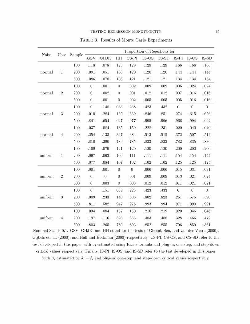
TESTING REGRESSION MONOTONICITY 65
Table 3. Results of Monte Carlo Experiments
Noise Case SampleProportion of Rejections for
GSV GHJK HH CS-PI CS-OS CS-SD IS-PI IS-OS IS-SD
100 .118 .078 .123 .129 .129 .129 .166 .166 .166
normal 1 200 .091 .051 .108 .120 .120 .120 .144 .144 .144
500 .086 .078 .105 .121 .121 .121 .134 .134 .134
100 0 .001 0 .002 .009 .009 .006 .024 .024
normal 2 200 0 .002 0 .001 .012 .012 .007 .016 .016
500 0 .001 0 .002 .005 .005 .005 .016 .016
100 0 .148 .033 .238 .423 .432 0 0 0
normal 3 200 .010 .284 .169 .639 .846 .851 .274 .615 .626
500 .841 .654 .947 .977 .995 .996 .966 .994 .994
100 .037 .084 .135 .159 .228 .231 .020 .040 .040
normal 4 200 .254 .133 .347 .384 .513 .515 .372 .507 .514
500 .810 .290 .789 .785 .833 .833 .782 .835 .836
100 .109 .079 .121 .120 .120 .120 .200 .200 .200
uniform 1 200 .097 .063 .109 .111 .111 .111 .154 .154 .154
500 .077 .084 .107 .102 .102 .102 .125 .125 .125
100 .001 .001 0 0 .006 .006 .015 .031 .031
uniform 2 200 0 0 0 .001 .009 .009 .013 .021 .024
500 0 .003 0 .003 .012 .012 .011 .021 .021
100 0 .151 .038 .225 .423 .433 0 0 0
uniform 3 200 .009 .233 .140 .606 .802 .823 .261 .575 .590
500 .811 .582 .947 .976 .993 .994 .971 .990 .991
100 .034 .084 .137 .150 .216 .219 .020 .046 .046
uniform 4 200 .197 .116 .326 .355 .483 .488 .328 .466 .472
500 .803 .265 .789 .803 .852 .855 .796 .859 .861
Nominal Size is 0.1. GSV, GHJK, and HH stand for the tests of Ghosal, Sen, and van der Vaart (2000),
Gijbels et. al. (2000), and Hall and Heckman (2000) respectively. CS-PI, CS-OS, and CS-SD refer to the
test developed in this paper with σi estimated using Rice’s formula and plug-in, one-step, and step-down
critical values respectively. Finally, IS-PI, IS-OS, and IS-SD refer to the test developed in this paper
with σi estimated by σi = εi and plug-in, one-step, and step-down critical values respectively.
Top Related