


Languages
Pages
Legal


Testing Portfolio Efficiency with Conditioning Information Wayne E. Ferson University of Southern California and NBER Andrew F. Siegel* University of Washington
First draft July 28, 2000, this revision: August 10, 2007
We develop asset pricing models’ implications for portfolio efficiency when there is
conditioning information in the form of a set of lagged instruments. A model of expected
returns identifies a portfolio that should be minimum variance efficient with respect to the
conditioning information. Our framework refines previous tests of portfolio efficiency by
using a given set of conditioning information optimally. The optimal use of the lagged
variables is economically important. With standard portfolio designs and lagged instruments,
by using the instruments optimally we reject several efficiency hypotheses that are not
otherwise rejected. The Sharpe ratios of a sample of hedge fund indexes appear consistent
with the optimal use of conditioning information.
*Wayne E. Ferson is Professor of Finance at the Marshall School, University of Southern California, 701 Exposition Blvd., Los Angeles, CA 90089-1427, phone (213) 740-5615. Andrew F. Siegel is the Grant I. Butterbaugh Professor of Finance and Business Economics, also of Information Systems and Operations Management, and is Adjunct Professor of Statistics, University of Washington, Box 353200, Seattle, WA. 98195-3200 [phone: (206)543-4476, fax: 685-9392, e-mail [email protected]]. This paper has benefited from comments of an anonymous referee and from Tom George, Jay Shanken and from workshops at the 2000 Pacific Northwest Finance Conference, the 2001 Western Finance Association, the Thirteenth Annual Conference on Financial Economics and Accounting/Fifth Maryland Finance Symposium (2002), the 2003 American Finance Association and at the following Universities: Arizona, Arizona State, the Copenhagen Business School, CUNY Baruch, INSEAD, Iowa, McGill, New York University, the Norwegian School of Economics, the Norwegian School of Business, Penn State, Toronto, Washington, and Wisconsin.
Testing Portfolio Efficiency with Conditioning Information
We develop asset pricing models’ implications for portfolio efficiency when there is
conditioning information in the form of a set of lagged instruments. A model of expected
returns identifies a portfolio that should be minimum variance efficient with respect to the
conditioning information. Our framework refines previous tests of portfolio efficiency by
using a given set of conditioning information optimally. The optimal use of the lagged
variables is economically important. With standard portfolio designs and lagged instruments,
by using the instruments optimally we reject several efficiency hypotheses that are not
otherwise rejected. The Sharpe ratios of a sample of hedge fund indexes appear consistent
with the optimal use of conditioning information.

1
Asset pricing models say that particular portfolios are minimum variance efficient, and testing
the efficiency of a given portfolio has long been an important topic in empirical asset pricing.1
Classical efficiency tests ask if a tested portfolio lies “significantly” inside a sample mean
variance boundary. These studies form the boundary from fixed-weight combinations of the
tested asset returns. However, many studies in asset pricing now use predetermined variables
to model conditional expected returns, correlations and volatility, and portfolio weights may
be functions of the predetermined variables. This paper develops tests of portfolio efficiency
in a conditional setting.
Our contribution is a new framework for testing asset pricing theories in the presence of
conditioning information. The framework uses “unconditional” efficiency as defined by
Hansen and Richard (1987). An unconditionally efficient portfolio uses the conditioning
information in the portfolio weight function, to minimize the unconditional variance of return
for its unconditional mean. We refer to this as (minimum variance) efficiency with respect to
the information, Z. By testing the implications of asset pricing models for efficiency with
respect to Z, we use the conditioning information “optimally,” allowing for nonlinear
functions of the information. Our testing framework has other attractive properties as well.
The basic logic of our approach is as follows. A model of expected returns implies that
for the right stochastic discount factor, m, E(mR|Z) = 1, where Z are observable lagged
1 The Capital Asset Pricing Model (CAPM, Sharpe, 1964) implies that a market portfolio should be mean variance efficient. Multiple-beta asset pricing models such as Merton (1973) imply that a combination of the factor portfolios is minimum variance efficient (Chamberlain, 1983; Grinblatt and Titman, 1987). The consumption CAPM implies that a maximum correlation portfolio for consumption is efficient (Breeden, 1979). More generally, any stochastic discount factor model implies that a maximum correlation portfolio for the stochastic discount factor is minimum variance efficient (e.g., Hansen and Richard, 1987). Classical efficiency tests are studied by Gibbons (1982), Jobson and Korkie (1982), Stambaugh (1982), MacKinlay (1987), Gibbons, Ross and Shanken (1989) and others.
2
instruments and R is the vector of gross (i.e., one plus the rate of) returns. Any specification
for m implies that particular portfolio(s) should be efficient with respect to Z. We test an asset
pricing model by testing the efficiency of the indicated portfolio(s) with respect to Z.
Our testing framework involves expanding the mean variance frontier through the use of
nonlinear “dynamic strategies,” as explained below. Therefore, a central empirical issue is
whether such strategies can improve the unconditional Sharpe ratio. For example, some
hedge funds claim large Sharpe ratios, and Fung and Hsieh (1997) find that hedge funds
follow nonlinear strategies. We find that an equity market neutral hedge fund index delivers
an average monthly Sharpe ratio of 0.76 during the 1995-2002 period. Static combinations of
the 25 Fama-French portfolios formed on size and book/market can only achieve a (bias
adjusted) Sharpe ratio of 0.31. However, by efficiently using standard lagged variables the
Sharpe ratio is 1.05. Thus, the economic significance of our approach is potentially large.
Hedge funds might appear to expand the mean variance boundary dramatically, but not when
the boundary includes the nonlinear lagged variable strategies.
Previous studies also use conditioning information to expand the set of returns. For
example, the “factors” or assets’ returns may be multiplied by lagged instruments, as in
Shanken (1990), Hansen and Jagannathan (1991), Cochrane (1996), Jagannathan and Wang
(1996) or Ferson and Schadt (1996). This “multiplicative” approach corresponds to dynamic
strategies whose portfolio weights are linear functions of the lagged instruments. However,
Ferson and Siegel (2001) show that the portfolio weight functions that maximize the Sharpe
ratio are not linear functions. They show (see their Figure 1) that the nonlinearities occur
within statistically reasonable limits.

3
Recent evidence calls into question the usefulness of standard lagged instruments to
predict asset returns, once bias and sampling errors are accounted for (e.g. Ghysels (1997),
Goyal and Welch (2003, 2004), Simin (2006), Ferson, Sarkissian and Simin, 2003).
However, these studies do not use the conditioning information optimally. We find that when
similar variables are used in the optimal nonlinear strategy they do have information.
In the standard approach, with N asset returns and L lagged instruments, a NL × NL
covariance matrix must be inverted. With our approach the matrices are N × N, so larger
problems with fewer time series can be handled. The main cost is the requirement to model
the conditional means and covariance matrix of returns. We evaluate this cost below.
Another advantage of our approach is robustness. Asset pricing tests can be misspecified
for various reasons. The econometrician can assume the wrong probability distribution,
misspecify the moments of the returns, or the returns can be measured with error. It is well
known that mean-variance portfolio solutions are especially sensitive to errors in estimating
the mean (e.g. Michaud, 1989). Since mean-variance analysis is the foundation of asset
pricing tests, errors in the means are particularly problematic. Our methods should be more
robust to these problems than the classical approach.2
The rest of the paper is organized as follows. Section 1 further motivates and presents the
main ideas. Section 2 develops the tests. The data are described in Section 3 and Section 4
presents the main empirical results. Section 5 concludes the paper.
2 Abhyankanar, Basu and Stremme (2006) and Chiang (2007) study the out-of-sample performance of the optimal portfolio strategies that form the basis our tests and find that they perform better than the standard mean variance solutions.

4
1. Asset Pricing, Portfolio Efficiency and Conditioning Information
Most asset pricing models can be represented using the fundamental valuation equation:
{ } 111
=++ tttZRmE , (1)
where Rt+1 is an N-vector of test asset gross returns, Zt is the conditioning information, a
vector of observable variables at time t, mt+1 is the stochastic discount factor (SDF) implied
by the model and 1 is an N-vector of ones. A common approach to testing an asset pricing
model is to examine necessary conditions of (1). For example, multiplying both sides of
Equation (1) by the elements of Zt and then taking the unconditional expectations leads to a
multiplicative approach:
( ){ } { }ttttZEZRmE !=!++ 1
11. (2)
Equation (2) asks the stochastic discount factor to “price” the dynamic strategy payoffs,
1t tR Z+ ! , on average (or “unconditionally”), where { }
tZE !1 are the average prices. The
multiplicative approach captures only a portion of the information in Equation (1). By using
“the right” functions of Zt we can capture more of the information. Of course, if the choice
of Z excludes important, unobserved information, this will result in a loss of power. In this
paper we take the choice of Z as given.
Equation (1) is equivalent to Equation (3), holding for all bounded integrable
functions f(.):
( ){ } { }1 1 1 ( )t t t tE m R f Z E f Z+ +! " =# $ . (3)
Equation (2) is a special case of (3), which may be seen by taking ( )tf Z to be each of the
instruments in turn and stacking the equations. Thus, Equation (2) asks the stochastic discount

5
factor to price only a subset of the strategies implied by Equation (1) and the asset pricing
model. Our tests use the following version of Equation (3):
{ }1 1'( ) 1 ( ) : '( )1 1t t t t t
E m x Z R x Z x Z+ + = ! = . (4)
Equation (4) uses all portfolio weight functions x(Z) in place of the general functions in
Equation (3), subject only to the restrictions that the weights are bounded integrable functions
that sum to 1.0.3
By using all portfolio weights in Equation (4), our approach rejects asset pricing models
that previous methods would not reject. While many asset pricing models are rejected in the
literature, Lewellen, Nagel and Shanken (2007) argue that it may be too easy to find models
that appear to “explain” some returns, like those of the Fama-French portfolios. Our approach
appears to be powerful in that setting.
Ferson and Siegel (2001) provide the expressions from which we construct the tests.
These describe the efficient frontier of all portfolio weight functions. The optimal weight
function minimizes the unconditional variance of 1'( )t t
x Z R + for its unconditional mean, µp,
3 Equation (4) follows by multiplying (1) by the elements of the portfolio weight vector ( )x Z and summing, using the fact that the weights sum to 1.0, then taking the unconditional expectation. Because of the portfolio weight restriction, Equation (4) is an implication of but is not equivalent to (3). Equation (4) retains the dynamic asset allocation decisions allowed by (3)—moving funds from one asset to another based on conditioning information—but leaves out the opportunity to save more or less, altering the overall scale of the investment based on conditioning information. In equation (3), since both sides of the equation may be arbitrarily scaled by a constant, the unconditional expectation of the portfolio weights sum to 1.0 (Abhyankar, Basu and Stremme, 2006). Restricting to weights that almost always sum to 1.0 in Equation (4) allows us to work with portfolio returns and portfolio efficiency, as opposed to asset prices and payoffs. Working with prices and payoffs, it would be necessary in any event, to normalize the prices to achieve stationarity for empirical work.
6
over the functions x(Z). The solution for the weights on the risky assets, in the presence of a
risk free asset with return Rf, is given by Ferson and Siegel (2001) as: 4
x(Z)' = [ ( ) 1]p f
fR
Z Rµ !
µ !"
' Q, (5)
where Q = 1
( ( ) 1)( ( ) 1) ( )f fZ R Z R Z!
"# $µ ! µ ! + %/& ' ,
and { ( ) 1) ( ( ) 1)}f fE Z R Q Z R!" = µ # µ # ,
and 1 is an N-vector of ones. We posit a parametric model for the conditional mean vector,
( )tZµ , and the conditional covariance matrix, ( )
tZ!/ . Note that even if the conditional mean
function is linear in Z, the optimal weight is nonlinear.
Ferson and Siegel (2001) study the shape of the optimal weight function of Equation (5).
They show that the portfolios are likely to be robust to extreme observations, because the
nonlinear shape makes them conservative in the face of extreme realizations of Zt. Ferson and
Siegel (2003) apply the expressions to the Hansen-Jagannathan (1991) bounds and find
robustness in that setting. Ferson, Siegel and Xu (2006) study modifications of the solutions
to compute maximum correlation portfolios and find evidence of robustness. Bekaert and Liu
(2004) argue that an approach like ours is inherently robust to misspecifying the conditional
moments of returns. The intuition is that with the wrong moments ( )tZµ and ( )
tZ!/ , using the
expression for the “optimal” x(Z) is suboptimal. However, the solution still describes a valid
portfolio strategy. The strategy will no longer expand the boundary to the maximum possible
4 Equation (5) applies when there is a fixed risk-free rate or a time-varying, conditionally risk-free rate. We have experimented with each interpretation and find that in our sample of returns and monthly Treasury bills, the two interpretations are virtually empirically indistinguishable.
7
extent. Thus the tests may sacrifice power, but remain valid with misspecified conditional
moments. The key to obtaining the advantages of our approach is the relation of Equation (4)
to minimum variance efficient portfolios.
1.1 Portfolio Efficiency with Respect to Conditioning Information
We first formally define efficiency with respect to the information, Zt. Consider the set of all
portfolios of the N test assets 1t
R + , where the weights ( )tx Z that determine the portfolio at
time t are functions of the given information tZ . The restrictions on the portfolio weight
function are that the weights must sum to 1.0 (almost surely in Zt), and that the expected value
and second moments of the portfolio return are well defined. This set of portfolio returns
determines a mean-standard deviation frontier, as shown by Hansen and Richard (1987). This
frontier depicts the unconditional means versus the unconditional standard deviations of the
portfolio returns. A portfolio is defined to be efficient with respect to the information Zt, when
it is on this mean standard deviation frontier.
Proposition 1. (Hansen and Richard, 1987, Corollary 3.1) Given N test asset gross returns,
Rt+1, a given portfolio with gross return p,t+1R is minimum-variance efficient with respect to
the information Zt if and only if Equation (6) (equivalently, Equation 7) is satisfied for all
t tx(Z ): x'(Z )1 1= almost surely, where the relevant unconditional moments exist and
are finite:
( ) ( ), 1 1p t t tVar R Var x Z R+ +!" #$ % & if ( ) ( ), 1 1p t t tE R E x Z R+ +
!" #= $ % (6)
( ) ( )1 0 1 1 , 1;t t t t p tE x Z R Cov x Z R R+ + +
! !" #" # = $ + $% & % & . (7)

8
Equation (6) is the definition of minimum variance efficiency with respect to Z. It states
that , 1p tR + is on the minimum variance boundary formed by all possible portfolios that use the
test assets and the conditioning information. Equation (7) states that the familiar expected
return - covariance relation from Fama (1973) and Roll (1977) must hold using efficient–
with-respect-to-Z portfolios. The expected returns on all the portfolio strategies are linear
functions of their unconditional covariances with Rp,t+1. In Equation (7), the coefficients 0!
and 1! are fixed scalars that do not depend on the functions x(.) or the realizations of
tZ .
1.2 Asset Pricing Models and Efficiency with Respect to Information
Most asset pricing models specify a stochastic discount factor. In particular, linear factor
models say that m is linear in one or more factors. Proposition 2 describes the simplest case of
our framework, showing that when there is conditioning information, testing linear factor
models amounts to testing for the efficiency of a portfolio of the factors with respect to the
information.
Proposition 2. Given {Rt+1, Zt} and a stochastic discount factor mt+1 such that Equation (4)
holds, then if t+1 B,t
m A B'R= ++1
, where RB,t+1 is a k-vector of benchmark factor returns,
and A and B are a constant and a fixed k-vector, there exists a portfolio, Rp,t+1 = w'RB,t+1,
w'1 = 1, where ( )w B/ 1 'B! is a constant k-vector, and Rp,t+1 is efficient with respect to the
information Zt.
Proof: See the Appendix for all proofs.

9
The intuition of Proposition 2 is the same as the classical case with no conditioning
information, as the proof in the appendix illustrates. The difference is that in our framework
the set of returns is expanded to all ( )'x Z R .
We are interested in general stochastic discount factors, m(X,θ), where X is observable
data and θ is a vector of parameters. We also wish to allow for time-varying weights in the
efficient portfolio. This requires the definition of portfolios that are maximum correlation
with respect to Z.
Definition. A portfolio RP is maximum correlation for a random variable, m, with
respect to conditioning information Z, iff:
( ) [ ]2 2, '( ) , ( ) : '( )1 1PR m x Z R m x Z x Z! " ! # = , (8)
where ρ2(.,.) is the squared unconditional correlation coefficient and we restrict to functions x
for which the correlation exists.
Proposition 3. If a given m satisfies Equation (4), then a portfolio RP that is maximum
correlation for m with respect to Z must be minimum variance efficient with respect to Z.
Proposition 2 is clearly a special case of Proposition 3, because a linear regression
maximizes the squared correlation. If mt+1 is linear in RB,t+1, a linear regression holds with no
error. We use Proposition 3 in our tests as follows. Given a stochastic discount factor, m, we
test the model by constructing a portfolio that is maximum correlation for this m with respect
to Z, and we then test the implication that the portfolio is efficient with respect to Z.5
5 To construct the maximum correlation portfolio for m with respect to Z, we form the portfolio weights using Equation (6) and the Corollary to Proposition 2 in Ferson, Siegel and Xu (2006).

10
With the preceding results we can consider a case where the model implies a stochastic
discount factor that is linear in k factor-portfolios, allowing for time-varying weights.
Corollary. Given {Rt+1, Zt} and a stochastic discount factor mt+1 such that Equation (4)
holds, then if a maximum correlation portfolio for mt+1 with respect to Zt has nonzero weights
only on the k-vector of benchmark factor returns B,t+1R , (a subset of Rt+1), then this portfolio
is efficient with respect to Z, both in the full set of test asset returns and in the benchmark
returns.
The situation described in the Corollary is a “dynamic” version of mean variance
“intersection,” as developed by Huberman, Kandel and Stambaugh (1987). The Corollary
follows because the factor portfolio in question satisfies the condition of Proposition 3, and so
is efficient with respect to Z, in both the full set and the subset of assets. Thus, the full set and
subset minimum variance boundaries must touch at the point defined by the maximum
correlation portfolio. The Corollary does not say that all efficient combinations of the factor
returns are efficient in the full set of returns. Other points on the subset boundary may be
inside the full set boundary.
1.3 Conditional Efficiency
Previous studies test conditional efficiency given Z, where efficiency is defined in terms of
the conditional means and variances.6 Tests of conditional efficiency given Z may be handled
6 Hansen and Hodrick (1983) and Gibbons and Ferson (1985) test versions of conditional efficiency given Z, assuming constant conditional betas. Campbell (1987) and Harvey (1989) test conditional efficiency restricting the form of a market price of risk, and Shanken (1990) and Ferson and Schadt (1996) restrict the form of time-varying conditional betas.

11
as a special case of our approach. If there is a (possibly, time-varying) combination of the k
benchmark returns, RB, that is conditionally efficient, there is an SDF, m = A(Z) + B(Z)'RB.
The coefficients are: ( ) ( ) ( ) ( )11 1| | 1 |f B B f BA Z R E R Z Cov R Z R E R Z!! !" # $= ! !% & and
( ) ( ) ( )1 1| 1 |B f BB Z Cov R Z R E R Z! !" #= !$ % . When 1k = we have a single-factor model, as in
the conditional CAPM. (See Ferson and Jagannathan, 1996.) We test conditional efficiency
by constructing the maximum correlation portfolio for the indicated m with respect to Z. This
portfolio, call it *pR , should be efficient with respect to Z. Note that *
pR will be different from
RB when the coefficients A(Z) or B(Z) are time varying functions of Z. Thus, for example, the
conditional CAPM does not imply that the market portfolio is efficient with respect to Z.
However, the conditional CAPM does identify a portfolio of the test assets that should be
efficient with respect to Z, and this can be tested using our approach.
If we reject conditional efficiency, then we reject dynamic intersection a fortiori. This
follows from the Hansen and Richard (1987) result that efficient-with-respect-to Z portfolios
must be conditionally efficient. If there is no combination of the benchmark returns that is
conditionally efficient, then no combination can be efficient with respect to Z, so there can be
no dynamic intersection.
2. Testing Efficiency

12
Classical tests of efficiency involve restrictions on the intercepts of a system of time-series
regressions. If tr is the vector of N excess returns at time t, measured in excess of a risk-free
or zero-beta return, and ,p tr is the excess return on the tested portfolio, the regression is:
,t p t t
r r u= ! +" + ; 1,...,t T= , (9)
where T is the number of time-series observations, β is the N-vector of betas and α is the N-
vector of alphas. The portfolio pr is minimum-variance efficient and has the given zero-beta
return only if ! =0.
Classical test statistics for the hypothesis that ! =0 can be written in terms of squared
Sharpe ratios (e.g., Jobson and Korkie, 1982). Consider the simplest case of the Wald
Statistic:
2 2
1
2
ˆ ˆ( ) ( )ˆ ˆ ˆ[ ( )]
ˆ1 ( )
p
p
S r S rW T Cov T
S r
!" #!
$= % % % = & '& '+( )
2~ ( )N!& (10)
where $! is the OLS or ML estimator of α and ( )T ! " !) converges to a normal random
vector with mean zero and covariance matrix, Cov( $ )! . The term ( )2ˆpS r is the sample value
of the squared Sharpe ratio of pr , defined by ( ) ( ) ( )
22
/p p pS r E r r! "= #$ % . The term ( )2S r is
the sample value of the maximum squared Sharpe ratio that can be obtained by portfolios of
the assets in r (including rp):
2
2 [ ( )]( ) max
( )x
E x rS r
Var x r
!" #= $ %
!& '. (11)

13
The Wald statistic has an asymptotic chi-squared distribution with N degrees of freedom
under the null hypothesis7.
Classical tests ignoring conditioning information restrict the maximization of Equation
(11) to fixed-weight portfolios, where x is a constant. Efficient portfolios with respect to the
information Z maximize the squared Sharpe ratio over all portfolio weight functions, ( )x Z .
2.1 Empirical Strategy
We compare the classical approach with no conditioning information, the multiplicative
approach, and the efficient use of the information. When we test the efficiency of a given
portfolio, Rp, then ( )2ˆpS R in the test statistic is formed using the normal maximum
likelihood estimators of the mean and variance. We use the one-month US Treasury bill
return as the risk-free or zero-beta rate.
The squared Sharpe ratio of the boundary portfolio, ( )2S R , differs according to the way
conditioning information is used. When there is no conditioning information we use the
fixed-weight solution to (11) evaluated at the maximum likelihood estimates. For the
multiplicative approach we use the returns 1)(ˆ!"!+= tfttftt ZRRRR , where Rft is the one-
month Treasury bill return for month t. We then proceed as in the fixed-weight case with the
returns tR in place of Rt. When the information is used efficiently, 2ˆ ( )S R is formed using the
7 When the Wald statistic in (10) is multiplied by !!"
#$$%
&
'
''
)2(
1
TN
NT , the result has an exact F distribution in finite
samples under the assumption that the (rt, rpt) in (9) are normally distributed (e.g., Gibbons, Ross and Shanken, (1989).

14
sample mean and variance of ˆ '( )x Z R where ˆ( )x Z is the sample version of the efficient-with-
respect-to-Z portfolio weight.
The solution for ˆ( )x Z is a function of the assumed parametric models for
1( ) ( )t t tZ E R Z+µ = and 1( ) ( )
t t tZ var R Z+! =/ . In the simplest examples ( )
tZµ is the linear
regression function for the returns on Z and ( )tZ!/ is the covariance matrix of the residuals,
which is held fixed over time. We also consider models with time-varying !/ (Zt).8
We evaluate the tests using simulations. To generate data consistent with the null
hypothesis that a portfolio is efficient, we either restrict the return generating process to
guarantee the portfolio’s efficiency, or we replace its return with a portfolio that is efficient,
based on the specification of the asset-return moments. We construct the null distribution of
the test statistic by using the artificial data in the same way that we use the actual data to get
the sample value of the statistic. The details are discussed in the Appendix.
We conduct experiments to assess the accuracy of our empirical p-values. With no lagged
instruments and normality the exact finite sample p-values are known from the F distribution
(footnote 7). We generate a random sample of normal returns from a population with mean and
covariance matrix equal to our ML sample estimates. The tested portfolio, which is the SP500, is
not efficient in this sample and the exact p-value from the F distribution is taken to be the
"correct" p-value. We check whether our simulations generate similar p-values. We replace the
SP500 with the portfolio that is efficient given the moments that generate the normal sample,
8 Previous approaches to conditional asset pricing directly specify ad-hoc functional forms for x(Z). We use the optimal strategies, which are given functions of ( )Zµ and ( )Z!/ , but we must specify these functions. Pushing the selection of the functional forms closer to the data is an improvement because the functional forms of asset return moments can be evaluated independently of portfolio performance.
15
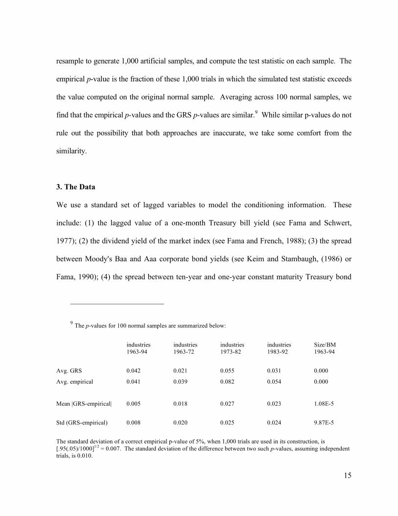
resample to generate 1,000 artificial samples, and compute the test statistic on each sample. The
empirical p-value is the fraction of these 1,000 trials in which the simulated test statistic exceeds
the value computed on the original normal sample. Averaging across 100 normal samples, we
find that the empirical p-values and the GRS p-values are similar.9 While similar p-values do not
rule out the possibility that both approaches are inaccurate, we take some comfort from the
similarity.
3. The Data
We use a standard set of lagged variables to model the conditioning information. These
include: (1) the lagged value of a one-month Treasury bill yield (see Fama and Schwert,
1977); (2) the dividend yield of the market index (see Fama and French, 1988); (3) the spread
between Moody's Baa and Aaa corporate bond yields (see Keim and Stambaugh, (1986) or
Fama, 1990); (4) the spread between ten-year and one-year constant maturity Treasury bond
9 The p-values for 100 normal samples are summarized below:
industries industries industries industries Size/BM 1963-94 1963-72 1973-82 1983-92 1963-94
Avg. GRS 0.042 0.021 0.055 0.031 0.000
Avg. empirical 0.041 0.039 0.082 0.054 0.000
Mean |GRS-empirical| 0.005 0.018 0.027 0.023 1.08E-5
Std (GRS-empirical) 0.008 0.020 0.025 0.024 9.87E-5
The standard deviation of a correct empirical p-value of 5%, when 1,000 trials are used in its construction, is [.95(.05)/1000]1/2 = 0.007. The standard deviation of the difference between two such p-values, assuming independent trials, is 0.010.

16
yields (see Fama and French, 1989) and (5); the difference between the one-month lagged
returns of a three-month and a one-month Treasury bill (see Campbell, 1987).
We use two standard methods of grouping monthly common stock returns into portfolios.
Twenty five value-weighted industry portfolios (from Harvey and Kirby, 1996) are used for
the period February, 1963 to December, 1994.10 Table 1 shows the SIC industry
classifications for the 25 portfolios, and summary statistics of the returns. The second
grouping follows Fama and French (1996). Stocks are placed into five groups according to
their prior equity market capitalization, and independently into five groups on the basis of
their ratios of book value to market value of equity per share. These are the same 25 portfolios
used by Ferson and Harvey (1999), who provide details and summary statistics.
This project has matured over a length of time, providing the opportunity to investigate
the results over a “hold-out” sample period, January, 1995 through December, 2002. We use
25 size x book-to-market and Industry portfolios from Kenneth French and update the other
series with fresh data.11 The hold-out sample results are interesting in view of recent
evidence, cited above, that some of the lagged instruments may have lost their predictive
power for stock returns since the 1990s. Table 1 reports the adjusted R-squares from
regressing the industry returns on the lagged instruments over the 1963-1994 period and the
1995-2002 sample. The R-squares are substantially lower in the more recent period.
10 We are grateful to Campbell Harvey for providing these data.
11 We use a subset of the 48 value-weighted industry portfolios provided by French to match the definitions in Table 1. We confirm that the matched industry returns produce similar summary statistics and regression R-squares on the lagged instruments as our original data, over the 1963-1994 period.

17
Regressions on the 25 size and book-to-market portfolios produces a similar result. The
average adjusted R-squared over 1963-1994 is 10.5%, while over 1995-2002 it is only 1.4%.
4. Empirical Results
4.1 Inefficiency of the SP500 Relative to Industry Portfolios
Table 2 summarizes results for the 25 industry portfolios, where the tested portfolio, pR , is
the SP500. In Panel A there is no conditioning information. Substituting the maximum
likelihood estimates of 2ˆ ( )pS R and 2ˆ ( )S R into (10) gives the sample value of the test
statistic. Referring to the asymptotic distribution, the right-tail p-value is 0.48 for 1964-94
and 0.14! 0.39 in the ten-year subperiods. These tests produce little evidence to reject the
null hypothesis. During 1995-2002 the maximum Sharpe ratio is substantially higher, and so
is the value of the test statistic: The asymptotic p-value is 0.001.
Panel A of Table 2 also reports 5% critical values and empirical p-values based on Monte
Carlo simulation assuming normality, and based on a resampling approach that does not
assume normality. In addition, we report p-values from the exact F statistic, under the
assumption of normality. Consistent with Gibbons, Ross and Shanken (GRS, 1989) the Wald
Test rejects too often when the asymptotic distribution is used, and when we correct for finite
sample bias using simulation we find no evidence against the efficiency of the market index in
the industry portfolios, at least when the conditioning information is ignored. The Monte
Carlo and bootstrapped p-values are close to each other in every subperiod, suggesting that
the departure from normality of the monthly industry returns is not severe. The p-values from
the F distribution are also similar to the empirical p-values.

18
Panel B of Table 2 summarizes tests using the “multiplicative” returns,
1)(ˆ!"!+= tfttftt ZRRRR . With 25 industry portfolios, the market return and five
instruments plus a constant (L=6), there are 156 “returns.” One disadvantage of the
multiplicative approach is that the size of the system quickly becomes unwieldy. It is not
possible to construct the Wald Test for the ten year subperiods, as the sample covariance
matrix is singular.
Over the 1963-94 period the value of the Wald Test statistic using the multiplicative
returns is 348.6. The asymptotic p-value is close to zero. However, we expect a finite-sample
bias and the simulations confirm the bias. The empirical p-values reject efficiency at either
the 2% (Monte Carlo) or 44% (resampling) levels. The Gibbons-Ross-Shanken p-value
assuming normality is 3%. Thus, the results in the multiplicative case are sensitive to the data
generating process. This makes sense, because even if Rt is approximately normal, the
products of returns and the elements of 1t
Z ! are not normal. We therefore place more trust in
the resampling results. Using the resampling scheme we find no evidence to reject the
efficiency of the market index with the multiplicative approach.
Panel C uses the conditioning information Z optimally. With this approach results for the
subperiods can be obtained. The empirical p-values are 0.5% or less in the full sample and
each ten-year subperiod, and 4.4% or less during 1995-2002. Thus, we reject the hypothesis
that the SP500 is efficient when using the conditioning information optimally. We even find
marginal rejections during the 1995-2002 sample period, where Table 1 illustrates that the
predictive power of the lagged instruments is low. The results based on the efficient-with-
respect-to-Z frontier are also fairly robust to the method of simulation (Monte Carlo or

19
resampling). This makes sense in view of the “robust” behavior of the portfolio weights that
define the efficient-with-respect-to-Z boundary, as described by Ferson and Siegel (2001).
4.2 Size and Book/Market Porfolios
Studies that use portfolios grouped on firm size and book-to-market ratios find that a market
index is not efficient (e.g. Fama and French, 1992). Table 3 presents results for these
portfolios. In panel A there is no conditioning information. Consistent with previous studies,
efficiency is rejected for the 1963-1994 period. However, in the 1995-2002 period, the
efficiency of the market index is not rejected when the finite sample bias in the statistics is
corrected. This is consistent with a weakening of the size and book-to-market effects during
1995-2002. In panel B the test assets are the multiplicative returns. The empirical p-value
based on resampling is marginal, at 4%, over the 1963-1994 sample.
In panel C the test assets are all portfolios ( )1t tx Z R!" . The resampling p-values are 0.3%
or less, including the 1995-2002 subsample. Thus, efficiency can be rejected with our
approach. Expanding the set of portfolio returns with the optimal nonlinear strategies changes
the results, even in the size × book-to-market portfolio design.
4.3 Expanding the Mean Variance Boundary
The above evidence shows that the market index return lies “significantly” inside the
mean-variance boundaries when the conditioning information is used optimally, but does not
address directly the relations between the boundaries formed with versus without the
information. Table 4 examines whether the use of conditioning information expands the
mean variance boundary. For these tests we replace the market index with a portfolio of the

20
test assets whose weights are proportional to 1!" µ/ , where !/ is the unconditional covariance
matrix and µ is the unconditional mean of the excess returns. This is a portfolio on the
simulations’ “population” mean-variance boundary with no conditioning information. We
then test for the efficiency of this portfolio instead of the SP500. In panel A we use the
multiplicative approach to expanding the boundary. The empirical p-values are 0.464 and
0.686, thus providing no evidence that the multiplicative approach expands the boundary.12
In Panel B of Table 4 the test assets are all portfolios ( )1t tx Z R!" . In the 1963-94 period
the empirical p-values are 0.1% and 2.5%, showing that when the conditioning information is
used optimally the mean variance boundary is expanded. However, during 1995-2002 we do
not reject the null hypothesis. This is the weakest showing that our new approach makes.
Note that the critical values are not drastically higher, but the sample values of the test
statistic are lower during 1995-2002. This reflects the low explanatory power of the lagged
variables during this period, as indicated in Table 1. The statistical noise involved in
estimating the maximum Sharpe ratio for the 26 test assets in this experiment differs from that
involving a smaller number of factors, so we may find rejections of other hypotheses during
the 1995-2002 period.
4.4 Testing Static Combinations of the Fama-French Factors
The null hypothesis may be stated as m = a + b1Rm + b2RHML + b3RSMB, where the coefficients
are fixed over time. Rm is the gross return of the market index. RHML is the one-month
12 Using a fixed risk-free rate these tests may sacrifice power, as there may be other regions, corresponding to other values of the zero-beta rate, where the two boundaries are reliably distinct.

21
Treasury bill gross return plus the excess return of high book-to-market over low book-to-
market stocks, and RSMB is similarly constructed using small and large market-capitalization
stocks. We replace the first and last portfolios in the industry or size × book-to-market design
with the returns RHML and RSMB, to insure that the factor portfolios are a subset of the tested
portfolio returns.
Table 5 presents the tests. Without conditioning information the only rejections occur for
the industry portfolios. The GRS and empirical p-values produce similar conclusions. Fama
and French (1997) also find that their factors don’t explain average industry returns very well.
In Panel B the multiplicative approach is used, and the empirical p-values strongly reject the
model for 1963-94. This is consistent with studies such as Ferson and Harvey (1999) who
find that the Fama-French factors do not explain time-varying expected returns over a similar
sample period. We cannot examine the multiplicative approach over the holdout sample
because the covariance matrices are too large to invert.
Panel C of Table 5 presents the tests relative to the efficient-with-respect-to-Z frontier.
The tests confirm the value of using the conditioning information optimally. We observe
strong rejections, both over 1963-1994 and in the 1995-2002 sample, and for both portfolio
designs.
4.5 Testing Time-Varying Combinations of Factors
In Table 6 we use our framework to test the conditional efficiency of the market index (Panel
A) and of time-varying combinations of the three Fama-French factors (Panel B). We reject
both models over 1963-1994 in both portfolio designs. The bootstrapped p-values are 1.2%
or less. We also reject both models in the 1995-2002 sample period with p-values of 1.8% or

22
less. Thus, when the conditioning information is used optimally our tests strongly reject
conditional versions of both the CAPM and the Fama-French three-factor model. If no time-
varying combination of the factors is conditionally efficient, then no time-varying
combination can be efficient with respect to Z. Thus, Table 6 rejects dynamic intersection a
fortiori.13
4.6 A Hedge Fund Example
This section fleshes out the hedge fund example from the introduction. We use monthly
returns for six hedge fund indexes from Credit Suisse/Tremont for the 1995-2002 period.
Panel A of Table 7 presents the Sharpe ratios, which vary from -0.05 to 0.76 across the fund
styles.
Fixed-weight combinations of the Fama-French portfolios and the CRSP value-
weighted market index produce a Sharpe ratio of only 0.72 (Panel B). Using industry
portfolios and the market, the maximum Sharpe ratio is 0.76 (Panel C). Sample Sharpe ratios
are known to be biased when N is large relative to T. Using the correction in Ferson and
Siegel (2003)14 the Sharpe ratios are 0.31 and 0.38. The hedge funds appear to offer
impressive Sharpe ratios in comparison. However, using the efficient-with-respect-to Z
portfolio weights the Sharpe ratios are 1.39 and 1.36 before adjustment, and 1.05 and 1.02
after adjustment.
13 We explicitly test dynamic intersection and confirm that it is rejected in all the sample periods and portfolio designs.
14 If the unadjusted squared Sharpe ratio is S, the adjusted squared ratio is S(T – N – 2)/T – N/T.

23
We test the null hypothesis that the hedge fund indexes offer no expansion of the mean
variance opportunity set. This says that the alphas in regression (9) are jointly zero when rp,t
is the efficient portfolio formed from the test assets, excluding the hedge funds. The test
statistic is Equation (10), which now compares the maximum Sharpe ratios attainable with
versus without the hedge funds. We strongly reject the null hypothesis using the fixed-weight
benchmark, with empirical p-values of 1.2% or less. Using the lagged variables optimally the
p-values range from 4.9% to 17.5%. Thus, while the hedge funds do expand the fixed-weight
boundary, the tests do not reject the hypothesis that the hedge fund returns could have been
generated with nonlinear strategies based on the lagged instruments.
5. Conclusions
We develop a framework for testing asset pricing models in the presence of lagged
conditioning information. Our tests examine the (unconditional) minimum variance efficiency
of a portfolio with respect to the conditioning information, a version of efficiency introduced
by Hansen and Richard (1987). Asset pricing models identify portfolios that should be
efficient with respect to the conditioning information, and by testing the efficiency of the
portfolio, we test the asset pricing model. We illustrate the approach with versions of the
Capital Asset Pricing model and the Fama-French (1996) factors.
Using a standard set of lagged instruments and test portfolios, the efficiency of all time-
varying combinations of the Fama-French factors is rejected. In the same setting, the
commonly-used “multiplicative” approach to conditioning information does not significantly
expand the mean variance boundary, nor can it reject all the models. The predictive power of
24
the lagged variables declines after 1995, but even during this period the optimal use of these
variables is economically and statistically significant.
Our paper suggests opportunities for future research. We use the Treasury bill return as
the risk-free rate. It should be interesting to apply our framework in a setting where the zero
beta rate is a parameter to be estimated, perhaps by extending results in Kandel (1984). Some
of our results use a maximum correlation, mimicking portfolio. It should be possible to study
models in which the correlation is less than the maximum, as would be implied by missing
assets, for example, perhaps by extending results in Kandel and Stambaugh (1989). Future
applications of our framework should also consider alternative test statistics, test assets, asset
pricing models and data generating processes. International asset pricing and portfolio
performance evaluation where nonlinearities may be important, such as for hedge funds,
could be especially interesting applications.
Appendix
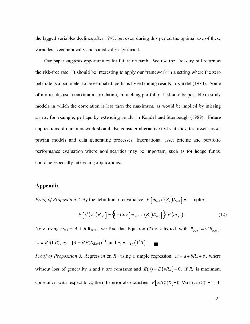
Proof of Proposition 2. By the definition of covariance, ( )1 11
t t tE m x Z R+ +
!" # =$ % implies
( ) ( ){ } ( )1 1 1 11 , /t t t t t t
E x Z R Cov m x Z R E m+ + + +! !" # " #= $% & % & . (12)
Now, using mt+1 = A + B′RB,t+1, we find that Equation (7) is satisfied, with , 1 , 1p t B tR w R+ +
!= ,
),'1/( BBw ! γ0 = [A + B'E(RB,t+1)]-1, and ( )1 01 B!" = #" . ▄
Proof of Proposition 3. Regress m on RP using a simple regression: P
m a bR u= + + , where
without loss of generality a and b are constants and ( )( ) 0P
E u E uR= = . If RP is maximum
correlation with respect to Z, then the error also satisfies: [ ]'( ) 0 ( ) : '( )1 1E ux Z R x Z x Z= ! = . If

25
this were not true for some ( )x Z , then ( )x Z R! enters an expanded regression with RP and
x'(Z)R on the right-hand side. Since the regression maximizes the squared correlation, this
would contradict the assumption that RP is maximum correlation. Substitute the simple
regression into (4) to obtain ( ) ( )P
E a bR u x Z R!" #+ +$ % = 1 = ( ) ( )P
E a bR x Z R!" #+$ %
11)(':)( =! ZxZx . Proposition 2 now establishes that RP is efficient with respect to Z. ▄
Evaluating the Tests by Simulation
Consider first a case with no conditioning information. For the Monte Carlo experiments we
draw from a normal distribution with mean vector and covariance matrix set equal to the ML
estimates for the sample period of the analysis. We replace the tested portfolio pR by a
portfolio whose weights maximize the Sharpe ratio at the ML estimates. The empirical 5%
critical value is the value above which 5% of the 1,000 simulated statistics lie. The empirical
p-value is the fraction of the 1,000 statistics that are larger than the value obtained in the
original sample.
We also resample using a parametric bootstrap approach. A regression of the returns on
the conditioning information defines the conditional mean function and the matrix of
residuals defines the unexpected returns. We choose randomly selected rows, with
replacement, from the matrix of residuals; the number of draws matches the length of the time
series. We use the conditional mean functions, evaluated at the simulated Z, and add the
independently resampled residuals to obtain the simulated returns.

26
We model Zt as a vector AR(1) process, and the sample AR(1) coefficient matrix is a
parameter of the simulations. We resample from the matrix of residuals of the AR(1) model
and build the time series of the Zt’s recursively.
When the null hypothesis places a given portfolio on the efficient-with-respect-to-Z
frontier, we replace the tested portfolio return with the time-varying combination of test assets
that is ex ante efficient given the data generating process (Tables 2 through 4). When the null
hypothesis specifies that a fixed weight combination of factors is efficient, we replace the first
factor with the ex ante efficient portfolio (Table 5). When the null hypothesis specifies the
conditional efficiency of a time-varying combination of the benchmark returns, RB, we replace
the conditional mean functions of the test assets with the expressions implied by the
conditional beta pricing restriction: 1 0( ) ( ) [ ]k
o j j BjZ Z E R Z=µ = ! + " # $ ! , where βj(Z) is the vector
of conditional betas on the j-th benchmark return (tables 6 and 8). In Table 7 we set the
alphas of the hedge funds on the efficient-with-respect-to Z portfolios equal to zero.
Conditional Heteroskedasticity
We evaluate the sensitivity of the tests to alternative specifications for conditional
heteroskedasticity in the returns. The "artificial analyst" in the simulations estimates the test
statistics as if the data were homoskedastic. The goal of these experiments is to see how our
inferences, based on the statistics that ignore heteroskedasticity, might be affected by
heteroskedasticity.
Since it may not be possible to agree on the right model for conditional heteroskedasticity,
we use two alternative approaches. In the first approach (method A) the heteroskedasticity is
driven by a factor, where the conditional betas on the common factor (the CRSP value-weighted

27
stock index return) are linear functions of the lagged instruments. The conditional betas, β(Z),
are estimated by regressing the unexpected asset returns on the index return and the products of
the index return with the lagged instruments. The time-varying beta is the regression coefficient
on the index plus the coefficients on the product terms multiplied by the lagged instruments. The
conditional covariance matrix is modeled as ( ) ( ) ( ) 2' fZ Z Z µ! = " " # + !/ / , where µ!/ is the fixed
covariance matrix of the factor model residuals and 2
f! is the fixed conditional variance of the
common factor, estimated from the residuals of its linear regression on the lagged Z.
The second approach to modeling heteroskedasticity (method B) follows Davidian and
Carroll (1987) and Ferson and Foerster (1994). The conditional standard deviations of the returns
are assumed to be linear functions. To estimate this model the absolute residuals from the linear
expected return models are regressed on the instruments. The fitted value, multiplied by / 2! ,
is the conditional standard deviation. The conditional covariances are modeled as the products of
the standard deviations and the fixed conditional correlations, where the correlations are
estimated from the residuals of the mean equations.
The models tested in Table 6 are evaluated under heteroskedastic data in Table 8. In
panels A and and B the null distribution is generated by method A. Panels C and D use the
linear conditional standard deviation approach, method B. The results of both approaches are
similar. When testing conditional efficiency the specification of the stochastic discount factor
changes under heteroskedasticity,15 but the effect is small. We experiment by computing the
15 Under conditional efficiency the stochastic discount factor is A(Z) + B(Z)'RB, and the coefficients A(Z) and B(Z) change when the data generating process changes.

28
sample values of the various test statistics, either using the heteroskedastic structure in the
calculations or ignoring it, and the sample values are not very sensitive to this choice.
References
Abhyankar, A., D. Basu, and A. Streme, 2007, “Portfolio Efficiency and Discount Factor Bounds with Conditioning Information: An Empirical Study,” Journal of Banking and Finance (forthcoming, 2007). Abhyankar, A., D. Basu, and A. Streme, 2006, “The optimal use of return predictability,” working paper, Warwick Business School . Bekaert, G, and J. Liu, 2004, “Conditioning Information and Variance Bounds on Pricing Kernels,” Review of Financial Studies 17, 339-378. Breeden, D.T., 1979, “An Intertemporal Asset Pricing Model with Stochastic Consumption and Investment Opportunities,” Journal of Financial Economics 7, 265-296. Campbell, John Y, 1987, “Stock returns and the Term Structure,” Journal of Financial Economics 18, 373-399. Chamberlain, G., 1983, “Funds, Factors and Diversification in Arbitrage Pricing Models,” Econometrica 51, 1305-1324. Chiang, Ethan, 2007, “Modern Portfolio Management with Information,” working paper, Boston College. Cochrane, J.H., 1996, “A Cross-Sectional Test of a Production Based Asset Pricing Model,” working paper, Journal of Political Economy. Davidian, M., and R.J. Carroll, 1987, “Variance Function Estimation,” Journal of the American Statistical Association, 82, 1079-1091. Fama, E.F., 1973, “A Note on the Market Model and the Two-Parameter Model,” Journal of Finance 28, 1181-1185. Fama, E.F., 1990, “Stock Returns, Expected Returns, and Real Activity,” Journal of Finance 45, 1089-1108. Fama, E.F., and K.R. French, 1988, “Dividend Yields and Expected Stock Returns,” Journal of Financial Economics 22, 3-25. Fama, E.F., and K.R. French, 1996, “Multifactor Explanations of Asset Pricing Anomalies,” Journal of Finance 51, 55-87.
29
Fama, E.F., and K.R. French, 1997, “Industry Costs of Equity,” Journal of Financial Economics 43, 15-193. Fama, E.F., and G.W. Schwert, 1977, “Asset Returns and Inflation,” Journal of Financial Economics 5, 115-146. Ferson, W.E., and S.R. Foerster, 1994, “Finite Sample Properties of the Generalized Method of Moments in Tests of Conditional Asset Pricing Models,” Journal of Financial Economics, 36, 29- 55. Ferson, W.E., and C.R. Harvey, 1999, “Conditioning Variables and the Cross-Section of Stock Returns,” Journal of Finance 54, 1325-1360. Ferson, W.E., and R. Jagannathan, 1996, “Econometric Evaluation of Asset Pricing Models,” In G.S. Maddala and C.R. Rao (eds.), The Handbook of Statistics, Volume 14 (Chapter One), Elsevier, New York. Ferson, W. E., and R.W. Schadt, 1996, “Measuring Fund Strategy and Performance in Changing Economic Conditions,” Journal of Finance 51, 425-462 . Ferson, W.E., S. Sarkissian, and T. Simin, 2003, “Spurious Regressions in Financial Economics?” Journal of Finance 58, 1393-1414. Ferson, W.E., and A.F. Siegel, 2001, “The Efficient Use of Conditioning Information in Portfolios,” Journal of Finance 56, 967-982. Ferson, W.E., and A.F. Siegel, 2003, “Stochastic Discount Factor Bounds with Conditioning Information,” Review of Financial Studies 16, 567-595. Ferson, W.E., and A.F. Siegel, 2007, “A note on the optimal orthogonal portfolio with conditioning information,” working paper, University of Southern California. Ferson, W.E., A.F. Siegel, and P. Xu, 2006, “Mimicking Portfolios with Conditioning Information,” Journal of Financial and Quantitative Analysis 41, 607-635. Fung, W. and D. Hsieh, 1997, Empirical characteristics of dynamic trading strategies: The case of hedge funds,” Review of Financial Studies 10, 275-302. Ghysels, E., 1997, “On Stable Factor Structures in the Pricing of Risk: Do Time-Varying Betas Help or Hurt?” Journal of Finance 53-549-573. Gibbons, M.R., 1982, “Multivariate Tests of Financial Models,” Journal of Financial Economics 10, 3-27. Gibbons, M.R., and W.E. Ferson, 1985, “Testing Asset Pricing Models with Changing Expectations and an Unobservable Market Portfolio,” Journal of Financial Economics 14, 217-236.

30
Gibbons, M.R., S.A. Ross, and J. Shanken, 1989, “A Test of the Efficiency of a Given Portfolio,” Econometrica 57, 1121-1152. Goyal, A., and I. Welch, 2003, “Predicting the Equity Premium with Dividend Ratios,” Management Science 49, 639-654. Goyal, A., and I. Welch, 2004, “A Comprehensive Look at the Empirical Performance of Equity Premium Prediction,” working paper, Emory University. Grinblatt, M., and S. Titman, 1987, “The Relation Between Mean-Variance Efficiency and Arbitrage Pricing,” Journal of Business 60, 97-112. Hansen, L.P, and R.J. Hodrick, 1983, “Risk Aversion Speculation in Forward Foreign Exchange Markets: An Econometric Analysis of Linear Models,” in J.A. Frenkel, (ed.) Exchange Rates and International Macro Economics, University of Chicago Press. Hansen, L.P., and R. Jagannathan, 1991, “Implications of Security Market Data for Models of Dynamic Economies,” Journal of Political Economy 99, 225-262. Hansen, L.P., and S.F. Richard, 1987, “The Role of Conditioning Information in Deducing Testable Restrictions Implied by Dynamic Asset Pricing Models,” Econometrica 55, No. 3, 587-613. Harvey, C.R., 1989, “Time-Varying Conditional Covariances in Tests of Asset Pricing Models,” Journal of Financial Economics 24, 289-318. Harvey, C.R., and C. Kirby, 1996, “Analytic Tests of Factor Pricing Models,” working paper, Duke University, Durham, N.C. Huberman, G., S. Kandel, and R. Stambaugh, 1987, “Mimicking Portfolios and Exact Arbitrage Pricing,” Journal of Finance 42, No. 1, 1-9. Jagannathan, R., and Z. Wang, 1996, “The Conditional CAPM and the Cross-Section of Expected Returns, Journal of Finance 51, 3-53. Jobson, J.D., and B. Korkie, 1982, “Potential Performance and Tests of Portfolio Efficiency,” Journal of Financial Economics 10, 433-466. Kandel, S.A., 1984, “The Likelihood Ratio Test Statistic of Mean Variance Efficiency Without a Riskless Asset,” Journal of Financial Economics 13, 575-592. Kandel, S.A., and R.F. Stambaugh, 1989, “A Mean-Variance Framework for Tests of Asset Pricing Models,” Review of Financial Studies 2, 125-156. Keim, D.B., and R.F. Stambaugh, 1986, “Predicting Returns in the Bond and Stock Markets,” Journal of Financial Economics 17, 357-390. Lewellen, J., S. Nagel and J. Shanken, 2007, “A skeptical appraisal of asset pricing tests,”

31
working paper, Emory University. MacKinlay, A.C., 1987, “On Multivariate Tests of the CAPM,” Journal of Financial Economics 18, 341-371. MacKinlay, A.C., 1995, “Multifactor Models Do Not Explain Deviations From the CAPM,” Journal of Financial Economics 38, 3-28. Merton, R., 1973, “An Intertemporal Capital Asset Pricing Model,” Econometrica 41, 867-887. Michaud, R., 1989, The Markowitz Optimization Enigma: Is optimized optimal?” Financial Analysts Journal 24 (January/February). Roll, R.R., 1985, “A Note on the Geometry of Shanken's CSR T2 Test for Mean/Variance Efficiency,” Journal of Financial Economics 14, 349-357. Roll, R., 1977, “A Critique of the Asset Pricing Theory's Tests - Part 1: On Past and Potential Testability of the Theory,” Journal of Financial Economics 4, 129-176. Shanken, J., 1987, “Multivariate Proxies and Asset Pricing Relations: Living with the Roll Critique,” Journal of Financial Economics 18, 91-110. Shanken, J., 1990, “Intertemporal Asset Pricing: An Empirical Investigation,” Journal of Econometrics 45, 99-120. Sharpe, W.F., 1964, “Capital Asset Prices: A Theory of Market Equilibrium Under Conditions of Risk,” Journal of Finance 19, 425-442. Simin, T., 2003, “The Poor Predictive Performance of Asset Pricing Models,” Journal of Financial and Quantitative Analysis (forthcoming). Stambaugh, R.F., 1982, “On the Exclusion of Assets from Tests of the Two-Parameter Model,” Journal of Financial Economics 10, 235-268. Treynor, J. and F. Black, 1973, “How to use Security Analysis to Improve Portfolio Selection, Journal of Business, 66-86.

Table 1. Monthly Industry Returns
--------------------------------------------------------------------------------------------------------------------------------------------- Industry SIC codes Mean σ ρ1
2R
2
HOLDOUTR
---------------------------------------------------------------------------------------------------------------------------------------------
1 Aerospace 372, 376 1.0107 0.0644 0.13 9.9 1.1 2 Transportation 40, 45 1.0094 0.0648 0.08 9.1 0.0 3 Banking 60 1.0086 0.0631 0.10 4.3 2.4 4 Building materials 24, 32 1.0097 0.0608 0.09 10.4 0.0 5 Chemicals/Plastics 281, 282, 286-289, 308 1.0094 0.0525 -0.01 8.0 2.5 6 Construction 15-17 1.0109 0.0760 0.16 10.2 0.0 7 Entertainment 365, 483, 484, 78 1.0135 0.0662 0.14 5.7 0.0 8 Food/Beverages 20 1.0117 0.0449 0.05 6.6 0.2 9 Healthcare 283, 384, 385, 80 1.0113 0.0524 0.01 2.4 0.0 10 Industrial Mach. 351-356 1.0089 0.0587 0.05 8.2 0.0 11 Insurance/Real Estate 63-65 1.0095 0.0581 0.15 6.4 2.3 12 Investments 62, 67 1.0097 0.0453 0.05 8.7 4.1 13 Metals 33 1.0075 0.0610 -0.02 4.5 0.2 14 Mining 10, 12, 14 1.0108 0.0535 0.01 7.2 0.3 15 Motor Vehicles 371, 551, 552 1.0095 0.0584 0.11 10.6 0.0 16 Paper 26 1.0095 0.0536 -0.02 6.9 2.4 17 Petroleum 13, 29 1.0102 0.0518 -0.02 4.4 0.0 18 Printing/Publishing 27 1.0114 0.0586 0.21 11.3 0.0 19 Professional Services 73, 87 1.0111 0.0693 0.13 8.4 2.8 20 Retailing 53, 56, 57, 59 1.0106 0.0597 0.15 8.7 3.7 21 Semiconductors 357, 367 1.0080 0.0559 0.08 9.0 0.0 22 Telecommunications 366, 381, 481, 482, 489 1.0085 0.0412 -0.05 5.4 8.8 23 Textiles/Apparel 22, 23 1.0100 0.0613 0.21 11.0 0.0 24 Utilities 49 1.0078 0.0392 0.02 6.8 4.3 25 Wholesaling 50, 51 1.0109 0.0614 0.13 10.7 0.0 ---------------------------------------------------------------------------------------------------------------------------------------------
Monthly returns on 25 portfolios of common stocks are from Harvey and Kirby (1996). The portfolios are value-weighted within each industry group, based on the SIC codes as shown. Mean is the sample mean of the gross (one plus rate of) return, σ is the sample standard deviation and !
1 is the first order autocorrelation
of the monthly return. 2R is the adjusted coefficient of determination in percent from the regression of the
returns on the lagged instruments. The sample period is February of 1963 through December of 1994 (383 observations). 2
HOLDOUTR is for the 1995-2002 holdout sample (96 observations). Negative adjusted R-
squares are reported as 0.0.

Table 2: Tests of the Mean Variance Efficiency of the Standard and Poors 500 Stock Index.
Subperiod 63-72 73-82 83-92 63-94 95-02 Panel A: Test assets Rt, no conditioning information: Wald Statistic 32.8 26.3 29.8 24.8 51.3 asymptotic p-value 0.14 0.39 0.23 0.48 0.001 GRS p-value 0.45 0.71 0.57 0.57 0.10 Monte Carlo 5% Critical Value 52.8 52.3 50.8 51.9 120.1 empirical p-value 0.43 0.71 0.58 0.59 0.44 Resampling 5% Critical Value 60.1 63.9 62.3 40.0 121.4 empirical p-value 0.52 0.81 0.65 0.58 0.49 Panel B: Test assets are 1)( !"!+ tfttft ZRRR :
Wald Statistic NA NA NA 348.6 NA asymptotic p-value 0.00 GRS p-value 0.03 Monte Carlo 5% Critical Value 328.0 empirical p-value 0.02 Resampling 5% Critical Value 476.0 empirical p-value 0.44 Panel C: Test assets are all Portfolios ( )1t t
x Z R!" :
Test Statistic 203.3 188.6 165.0 161.8 148.2 Monte Carlo 5% Critical Value 125.7 121.6 121.6 133.3 139.9 empirical p-value 0.000 0.000 0.001 0.002 0.029 Resampling 5% Critical Value 117.3 130.6 121.6 118.8 144.9 empirical p-value 0.003 0.005 0.003 0.001 0.044 The monthly returns on 25 industry-sorted portfolios of common stocks are test assets for February 1963 through December 1994 (T=383 observations), and ten-year subperiods. A holdout sample from January, 1995 through December, 2002 (96 observations) is also shown. The conditioning information consists of a lagged Treasury bill yield, dividend yield, excess bill return, and yield spreads of long over short-term Government bonds and low-grade over high-grade corporate bonds. NA denotes not applicable, when the number of assets is larger than the number of time series observations. Asymptotic p-values are from the chi-squared distribution. GRS p-values are from the F distribution, after the test statistic is rescaled to have an exact F distribution assuming normality as in Gibbons, Ross, and Shanken (1989).

Table 3: Tests of the Mean Variance Efficiency of the Standard and Poors 500 Stock
Index in Size and Book/Market Portfolios.
Sample size/BM industry 63-94 95-02 63-94 95-02 Panel A: No conditioning information: Sample Statistic 83.0 74.1 24.8 51.3 GRS p-value 0.000 0.007 0.57 0.102 Resampling 5% Critical Value 45.1 131.5 40.0 121.4 Empirical p-value 0.000 0.277 0.58 0.49 Panel B: Test assets are 1)( !"!+ tfttft ZRRR : Sample Statistic 517.1 NA 348.6 NA Resampling 5% Critical Value 508.8 476.0 Empirical p-value 0.040 0.44 Panel C: Test assets are all Portfolios ( )1t t
x Z R!" :
Sample Statistic 272.7 210.4 161.8 148.2 Resampling 5% Critical Value 107.6 135.1 118.8 144.9 Empirical p-value 0.000 0.003 0.001 0.044
The size/BM returns are 25 portfolios of stocks sorted on market capitalization and book-to-market ratio, for the sample period July 1963 through December 1994 (T=378 observations). A holdout sample covers January 1995 through December, 2002 (96 observations). The conditioning information consists of a lagged Treasury bill yield, dividend yield, excess bill return, and yield spreads of long over short-term Government bonds and low-grade over high-grade corporate bonds. NA indicates that the sample size does not allow the statistic to be calculated.

36
Table 4: Tests of the Hypothesis that Conditioning Information does not Expand the
Mean Variance Boundary.
size/BM industry 63-94 95-02 63-94 95-02 Panel A: Test assets are 1)( !"!+ tfttft ZRRR : Sample Statistic 356.3 NA 304.3 NA Resampling 5% Critical Value 520.4 486.0 Empirical p-value 0.464 0.686 Panel B: Test assets are all Portfolios ( )1t t
x Z R!" :
Sample Statistic 155.8 77.7 128.8 63.8 Resampling 5% Critical Value 108.7 138.3 118.8 148.1 Empirical p-value 0.001 0.539 0.025 0.779
The industry data are monthly returns on 25 industry-sorted portfolios of common stocks and a market index return. The size/BM returns are for 25 portfolios of stocks sorted on market capitalization and book-to-market ratios and a market index return. The conditioning information consists of a lagged Treasury bill yield, dividend yield, excess bill return, and yield spreads of long over short-term Government bonds and low-grade over high-grade corporate bonds. NA indicates that the sample size does not allow the test statistic to be calculated.

37
Table 5: Tests of the Efficiency of Fixed-weight Combinations of the Fama-French
Factors.
size/BM industry 63-94 95-02 63-94 95-02 Panel A: Test assets are Rt: Sample Statistic 35.0 49.5 43.0 55.5 GRS p-value
0.154 0.123 0.035 0.064
Resampling 5% Critical Value 41.6 64.0 39.2 61.2 empirical p-value 0.117 0.157 0.021 0.077 Panel B: Test assets are all Portfolios 1)( !"!+ tfttft ZRRR : Sample Statistic 521.9
NA 415.0
NA
Resampling 5% Critical Value 319.3 NA 313.7 NA empirical p-value 0.000 0.000 Panel C: Test assets are ( )1t t
x Z R!" :
Sample Statistic 340.6 181.6 180.1 174.6 Resampling 5% Critical Value 70.5 128.0 75.6 118.4 empirical p-value 0.000 0.003 0.000 0.001
The industry data are monthly returns on 25 industry-sorted portfolios of common stocks and a value-weighted index. The size/BM returns are for 25 portfolios of stocks sorted on market capitalization and book-to-market ratio and a value-weighted return. In each design the first and 25th portfolio returns are replaced with the returns of the HML and SMB factors, respectively. The conditioning information consists of a lagged Treasury bill yield, dividend yield, excess bill return, and yield spreads of long over short-term Government bonds and low-grade over high-grade corporate bonds. NA indicates that the sample size does not allow the test statistic to be calculated.

38
Table 6: Tests of Conditional Efficiency.
size/BM industry 63-94 95-02 63-94 95-02 Panel A: Conditional Efficiency of the Market Index Sample Statistic 339.2 131.7 189.7 143.0 Resampling 5% Critical Value 116.1 83.4 98.8 86.4 Empirical p-value 0.000 0.011 0.002 0.011 Panel B: Conditional Efficiency of the Fama-French Factors Sample Statistic 347.3 138.7 147.5 142.1 Resampling 5% Critical Value 67.3 95.0 71.2 99.1 Empirical p-value 0.000 0.012 0.000 0.018
The industry data are monthly returns on 25 industry-sorted portfolios of common stocks and a market index return. The size/BM returns are for 25 portfolios of stocks sorted on market capitalization and book-to-market ratios and a market index. In each design the first and 25th portfolio returns are replaced with the returns of the HML and SMB factors. The conditioning information consists of a lagged Treasury bill yield, dividend yield, excess bill return, and yield spreads of long over short-term Government bonds and low-grade over high-grade corporate bonds.

39
Table 7: The Efficiency of Hedge Funds Sharpe
Ratio Adjusted Sharpe
Panel A: Hedge Fund Indexes Convertible Arbitrage 0.49 0.49 Dedicated Short Bias Equity Market Neutral Event Driven Long/Short Equity Hedge Fund Index
-0.05 0.76 0.32 0.24 0.26
-0.05 0.76 0.31 0.23 0.26
Panel B: Size and B/M Portfolios and Market Index Fixed-weight Benchmark: Sharpe ratios Empirical p-value
0.72 0.002
0.31 0.001
Efficient wrt.Z benchmark Sharpe ratios Empirical p-values
1.39 0.052
1.05 0.049
Panel C: Industry Portfolios and Market Index Fixed-weight Benchmark: Sharpe ratios Empirical p-value
0.76 0.009
0.38 0.012
Efficient wrt.Z benchmark Sharpe ratios Empirical p-values
1.36 0.171
1.02 0.175
The indexes of hedge funds are monthly total returns from Credit Suisse/Tremont. The industry portfolios are monthly returns on 25 industry-sorted portfolios of common stocks and a market index return. The size/BM returns are for 25 portfolios of stocks sorted on market capitalization and book-to-market ratios and a market index. In each design the first and 25th portfolio returns are replaced with the returns of the HML and SMB factors. The conditioning information consists of a lagged Treasury bill yield, dividend yield, excess bill return, and yield spreads of long over short-term Government bonds and low-grade over high-grade corporate bonds.

40
Table 8: The Impact of Conditional Heteroskedasticity.
size/BM industry 63-94 95-02 63-94 95-02 Panel A: Conditional Efficiency of the Market Index – Method A Sample Statistic 344.5 131.4 184.9 144.3 Resampling 5% Critical Value 48.8 80.3 56.8 84.0 Empirical p-value 0.000 0.010 0.000 0.005 Panel B: Conditional Efficiency of the Fama-French Factors – Method A Sample Statistic 357.2 145.4 145.5 148.5 Resampling 5% Critical Value 66.7 94.2 70.0 89.6 Empirical p-value 0.000 0.004 0.000 0.007 Panel C: Conditional Efficiency of the Market Index – Method B Sample Statistic 371.3 152.5 211.3 158.4 Resampling 5% Critical Value 84.6 89.8 79.2 86.9 empirical p-value 0.000 0.000 0.000 0.000 Panel D: Conditional Efficiency of the Fama-French Factors – Method B Sample Statistic 371.3 174.5 152.2 174.4 Resampling 5% Critical Value 79.9 117.5 90.5 108.7 empirical p-value 0.000 0.002 0.004 0.003
The simulated data incorporate conditional heteroskedasticity either through a factor model with conditional betas that are linear functions of the lagged instruments (method A) or through a model in which the conditional standard deviations are linear functions of the conditioning variables and the conditional correlations are constant over time (method B). The industry data are monthly returns on 25 industry-sorted portfolios of common stocks and a market index return. The size/BM returns are for 25 portfolios of stocks sorted on market capitalization and book-to-market ratios and a market index. In each design the first and 25th portfolio returns are replaced with the returns of the HML and SMB factors. The conditioning information consists of a lagged Treasury bill yield, dividend yield, excess bill return, and yield spreads of long over short-term Government bonds and low-grade over high-grade corporate bonds.
Top Related