


Languages
Pages
Legal


Biomedical Information Systems ISC 471 / HCI 571 Fall 2012
How to Use SPSS for Classification
This handout explains how to use SPSS for classification tasks. We will see three methods for classification tasks, and how to interpret the results: binary logistic regression, multinomial regression, and nearest neighbor.
Binary Logistic Regression
Input data characteristicsIt assumes that the dependent variable is dichotomic (Boolean). The independent variables (predictors) are either dichotomic or numeric.It is recommended to have at least 20 cases per predictor (independent variable).
Steps to run in SPSS1. Select Analyze Regression Binary Logistic.
2. Select the dependent variable and the independent variables, and the selected method (Enter for example, which is the default).
1

Biomedical Information Systems ISC 471 / HCI 571 Fall 2012
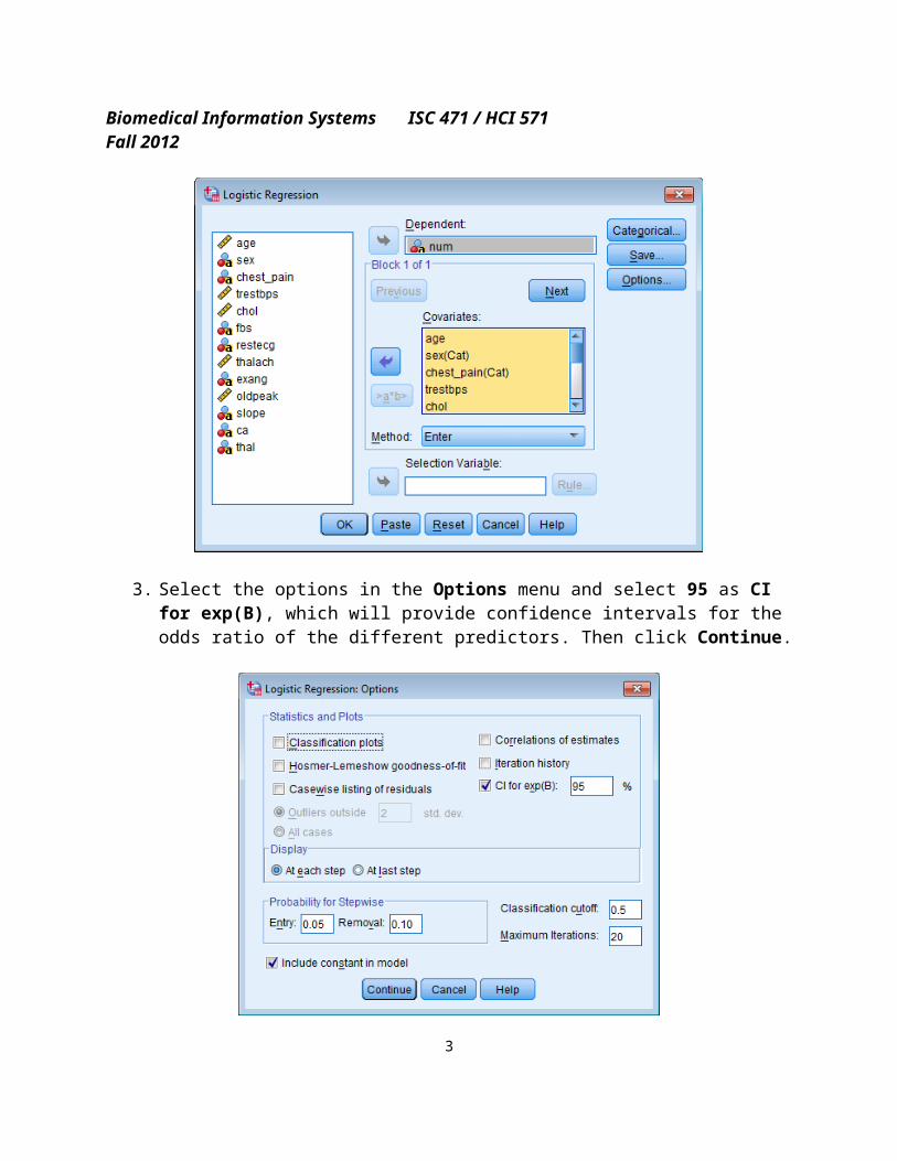
3. Select the options in the Options menu and select 95 as CI for exp(B), which will provide confidence intervals for the odds ratio of the different predictors. Then click Continue.
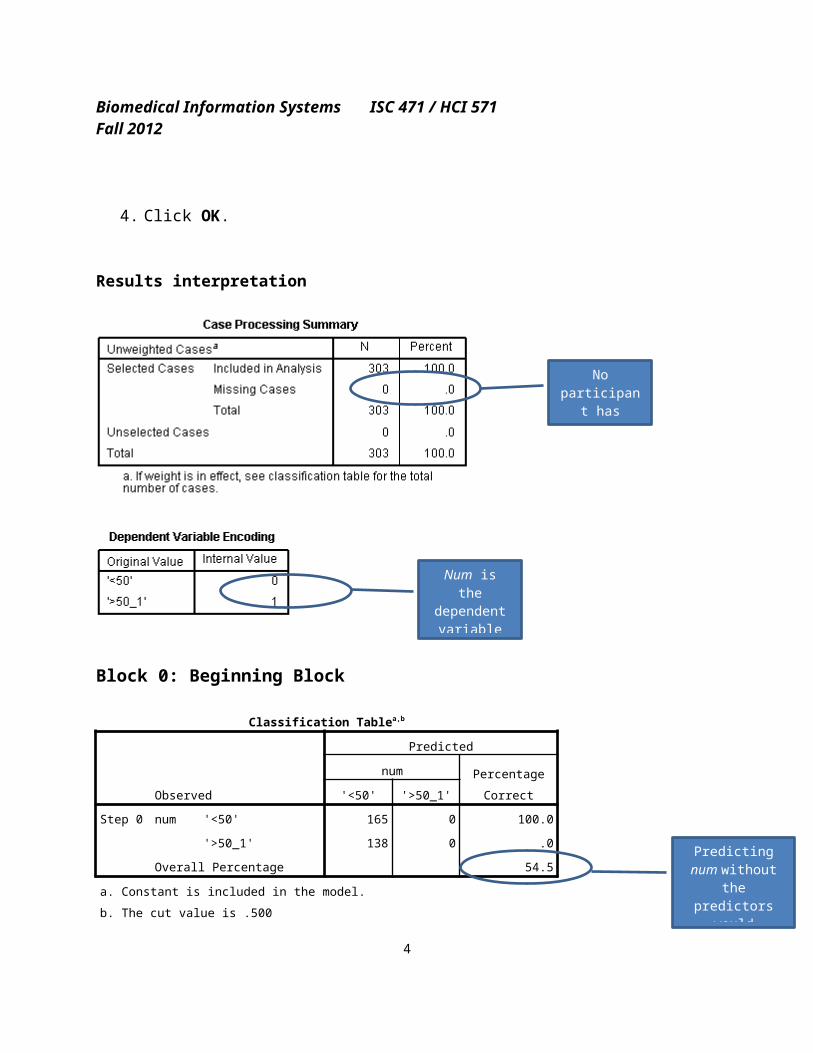
4. Click OK.
2
Biomedical Information Systems ISC 471 / HCI 571 Fall 2012
Results interpretation
Block 0: Beginning Block
Classification Tablea,b
Observed
Predicted
num Percentage
Correct'<50' '>50_1'
Step 0 num '<50' 165 0 100.0
'>50_1' 138 0 .0
Overall Percentage 54.5
a. Constant is included in the model.
b. The cut value is .500
Without using the predictors, we could predict that no participant has heart disease with 54.3%
accuracy – which is not significantly different from 50-50 (i.e, no better than chance).
Variables not in the Equation
Score df Sig.
No participant has missing
data
Num is the dependent
variable and is coed 0 or 1
Predicting num without the
predictors would provide 54.3%
accuracy
3
Biomedical Information Systems ISC 471 / HCI 571 Fall 2012
Step 0 Variables age 15.399 1 .000
sex(1) 23.914 1 .000
chest_pain 81.686 3 .000
chest_pain(1) 80.680 1 .000
chest_pain(2) 18.318 1 .000
chest_pain(3) 30.399 1 .000
trestbps 6.365 1 .012
chol 2.202 1 .138
fbs(1) .238 1 .625
restecg 10.023 2 .007
restecg(1) 7.735 1 .005
restecg(2) 9.314 1 .002
thalach 53.893 1 .000
exang(1) 57.799 1 .000
oldpeak 56.206 1 .000
slope 47.507 2 .000
slope(1) 1.224 1 .269
slope(2) 39.718 1 .000
ca 74.367 4 .000
ca(1) 1.338 1 .247
ca(2) 65.683 1 .000
ca(3) 16.367 1 .000
ca(4) 22.748 1 .000
thal 85.304 3 .000
thal(1) .016 1 .899
thal(2) 3.442 1 .064
thal(3) 84.258 1 .000
Overall Statistics 176.289 22 .000
Many variables are separately significantly related to num. All variables with Sig. less than or
equal to 0.05 are significant predictors of whether a person has heart disease. There are 11 of
these significant predictors here: age, sex, chest_pain, trestbps, restecg, thalach, exang, oldpeak,
slope, ca, thal.
Age is significantly
related to num.
4

Biomedical Information Systems ISC 471 / HCI 571 Fall 2012
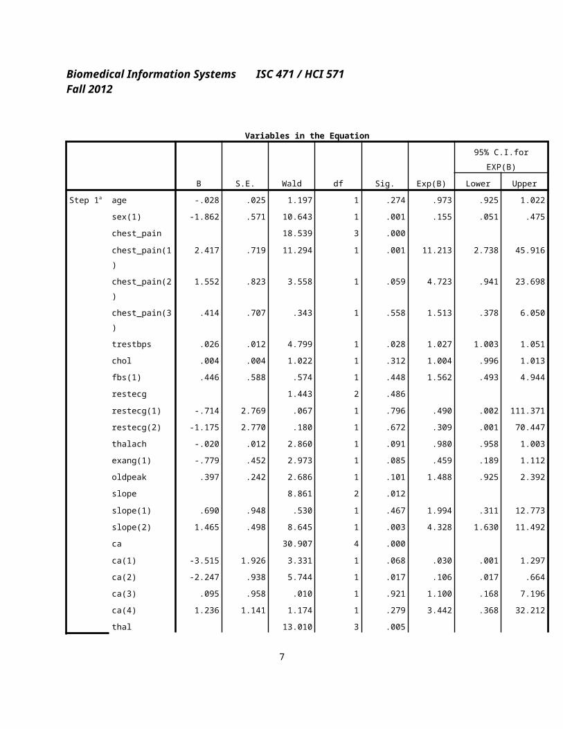
Block 1: Method = Enter
Variables in the Equation
B S.E. Wald df Sig. Exp(B)
95% C.I.for EXP(B)
Lower Upper
Step 1a age -.028 .025 1.197 1 .274 .973 .925 1.022
sex(1) -1.862 .571 10.643 1 .001 .155 .051 .475
chest_pain 18.539 3 .000
chest_pain(1) 2.417 .719 11.294 1 .001 11.213 2.738 45.916
chest_pain(2) 1.552 .823 3.558 1 .059 4.723 .941 23.698
chest_pain(3) .414 .707 .343 1 .558 1.513 .378 6.050
trestbps .026 .012 4.799 1 .028 1.027 1.003 1.051
The model is significant when all independent
variables are entered (Sig <=
0.05).
72.7% of the variance in num can be predicted
from the combination of the
independent variables.
88.4% of the subjects were
correctly classified by the model.
5

Biomedical Information Systems ISC 471 / HCI 571 Fall 2012
chol .004 .004 1.022 1 .312 1.004 .996 1.013
fbs(1) .446 .588 .574 1 .448 1.562 .493 4.944
restecg 1.443 2 .486
restecg(1) -.714 2.769 .067 1 .796 .490 .002 111.371
restecg(2) -1.175 2.770 .180 1 .672 .309 .001 70.447
thalach -.020 .012 2.860 1 .091 .980 .958 1.003
exang(1) -.779 .452 2.973 1 .085 .459 .189 1.112
oldpeak .397 .242 2.686 1 .101 1.488 .925 2.392
slope 8.861 2 .012
slope(1) .690 .948 .530 1 .467 1.994 .311 12.773
slope(2) 1.465 .498 8.645 1 .003 4.328 1.630 11.492
ca 30.907 4 .000
ca(1) -3.515 1.926 3.331 1 .068 .030 .001 1.297
ca(2) -2.247 .938 5.744 1 .017 .106 .017 .664
ca(3) .095 .958 .010 1 .921 1.100 .168 7.196
ca(4) 1.236 1.141 1.174 1 .279 3.442 .368 32.212
thal 13.010 3 .005
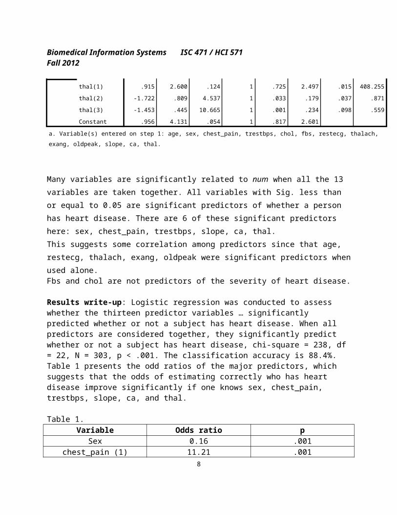
thal(1) .915 2.600 .124 1 .725 2.497 .015 408.255
thal(2) -1.722 .809 4.537 1 .033 .179 .037 .871
thal(3) -1.453 .445 10.665 1 .001 .234 .098 .559
Constant .956 4.131 .054 1 .817 2.601
a. Variable(s) entered on step 1: age, sex, chest_pain, trestbps, chol, fbs, restecg, thalach, exang, oldpeak, slope, ca, thal.
Many variables are significantly related to num when all the 13 variables are taken together. All
variables with Sig. less than or equal to 0.05 are significant predictors of whether a person has
heart disease. There are 6 of these significant predictors here: sex, chest_pain, trestbps, slope, ca,
thal.
This suggests some correlation among predictors since that age, restecg, thalach, exang, oldpeak
were significant predictors when used alone. Fbs and chol are not predictors of the severity of heart disease.
Results write-up: Logistic regression was conducted to assess whether the thirteen predictor variables … significantly predicted whether or not a subject has heart disease. When all
6
Biomedical Information Systems ISC 471 / HCI 571 Fall 2012
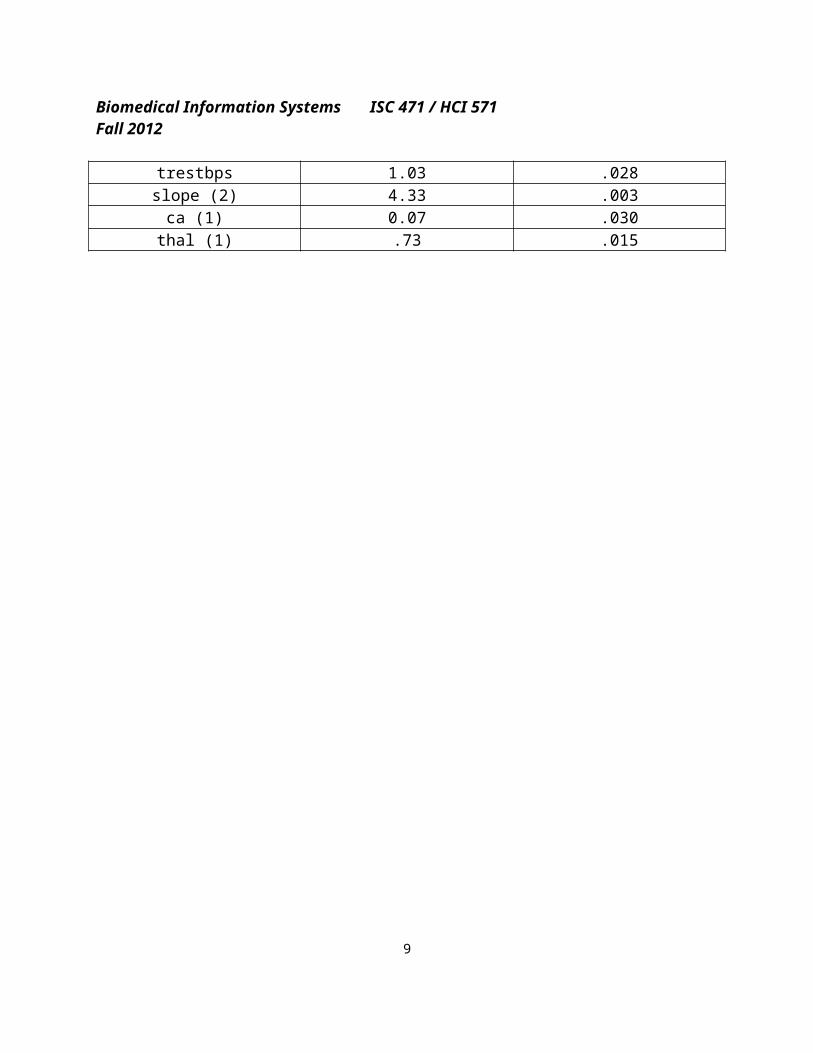
predictors are considered together, they significantly predict whether or not a subject has heart disease, chi-square = 238, df = 22, N = 303, p < .001. The classification accuracy is 88.4%. Table 1 presents the odd ratios of the major predictors, which suggests that the odds of estimating correctly who has heart disease improve significantly if one knows sex, chest_pain, trestbps, slope, ca, and thal.
Table 1.Variable Odds ratio p
Sex 0.16 .001chest_pain (1) 11.21 .001
trestbps 1.03 .028slope (2) 4.33 .003
ca (1) 0.07 .030thal (1) .73 .015
7
Biomedical Information Systems ISC 471 / HCI 571 Fall 2012
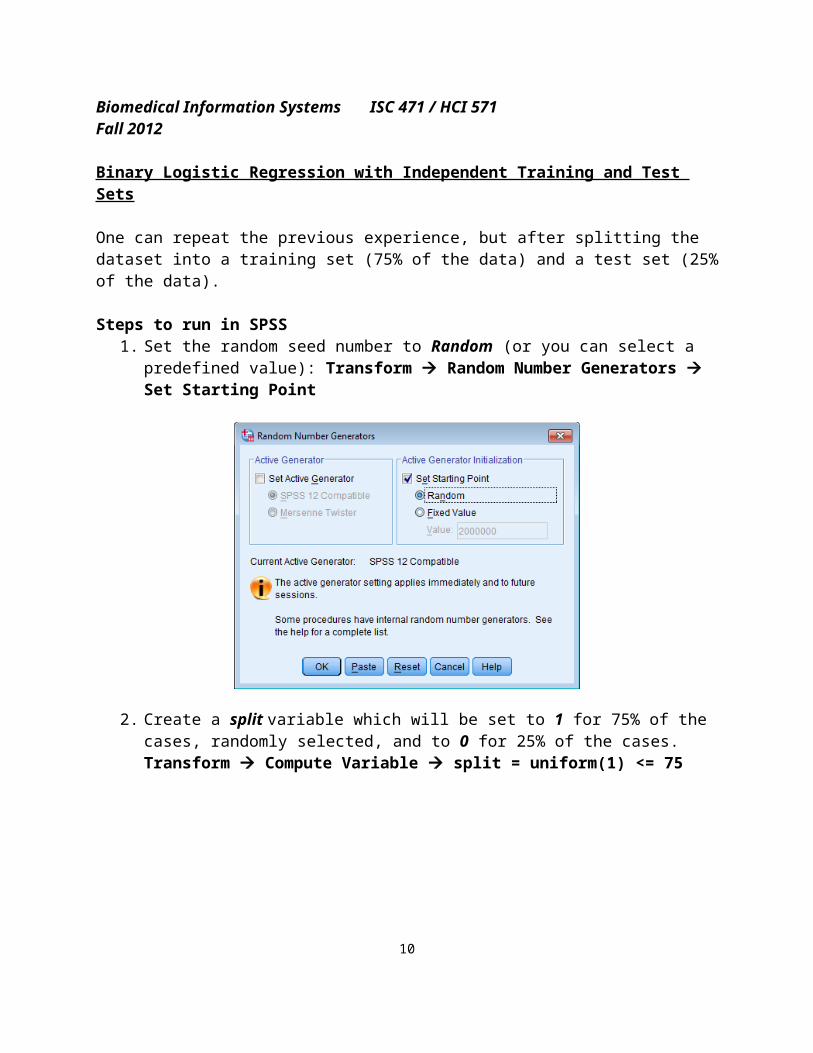
Binary Logistic Regression with Independent Training and Test Sets
One can repeat the previous experience, but after splitting the dataset into a training set (75% of the data) and a test set (25% of the data).
Steps to run in SPSS1. Set the random seed number to Random (or you can select a predefined value):
Transform Random Number Generators Set Starting Point
2. Create a split variable which will be set to 1 for 75% of the cases, randomly selected, and to 0 for 25% of the cases.Transform Compute Variable split = uniform(1) <= 75
8
Biomedical Information Systems ISC 471 / HCI 571 Fall 2012
3. Recall the Logistic Regression experiment from the Recall icon.
9
Biomedical Information Systems ISC 471 / HCI 571 Fall 2012
4. Repeat the regression as before, except that the Selection Variable is chosen as the split variable and the value 1 is selected for this variable under Rule.
5. Click on OK to run the Binary Logistic regression.
Results interpretation
Block 1: Method = Enter
10

Biomedical Information Systems ISC 471 / HCI 571 Fall 2012
The classification rate in the holdout sample is within 10% of the training sample(87.4% * 0.9).This is sufficient evidence of the utility of the logistic regression model.
The 6 significant predictors are the same: sex, chest_pain, trestbps, slope, ca, thal.
Results write-up: By splitting the dataset into 75% training set and 25% test set, the accuracy in the holdout sample changes to 85.0%, which is within 10% of the training sample. The significant predictors remain the same as in the model of the entire dataset. These results reinforce the utility of the logistic regression model.
The model is significant when all independent
variables are entered (Sig <
0.01).
72.7% of the variance in num can be predicted
from the combination of the
independent variables.
85.0% of the test subjects were
correctly classified by the model.
11

Biomedical Information Systems ISC 471 / HCI 571 Fall 2012
Nearest Neighbor
Input data characteristicsIt assumes that the dependent variable is dichotomic (Boolean). The independent variables (predictors) are either dichotomic or numeric.It is recommended to have at least 20 cases per predictor (independent variable).
Steps to run in SPSS1. Select Analyze Classify Nearest Neighbor.
2. Select the target variable and the features (or factors).
12

Biomedical Information Systems ISC 471 / HCI 571 Fall 2012
3. You may change other options, such as the number of neighbors (Neighbors tab), the distance metric, feature selection (Features tab), and the Partitions (Partitions tab). We select here to split the training set (75%) and the test set (25%).Other options on this page are the 10-fold cross validation, which yields a more robust evaluation.
13

Biomedical Information Systems ISC 471 / HCI 571 Fall 2012
14

Biomedical Information Systems ISC 471 / HCI 571 Fall 2012
4. Click OK.
Results interpretation
The classification accuracy is found in the model viewer by double-clicking the chart obtained and looking at the classification table, which shows an accuracy of 87.2% for K = 5.
Classification Table
Partition ObservedPredicted
'<50' '>50_1' Percent Correct
Training'<50' 100 16 86.2%'>50_1' 23 78 77.2%Overall Percent 56.7% 43.3% 82.0%
Holdout '<50' 43 6 87.8%'>50_1' 5 32 86.5%
15

Biomedical Information Systems ISC 471 / HCI 571 Fall 2012
Missing 0 0Overall Percent 55.8% 44.2% 87.2%
Results write-up: Nearest neighbor classification with k= 3 (3NN) was conducted to assess whether the thirteen predictor variables correctly predicted whether or not a subject has heart disease. When all predictors are considered together, 87.2% of the subjects were correctly classified.
Classification accuracy.
16
Top Related