


![Arnold and Commissioner of Taxation (Taxation) … and Commissioner of Taxation (Taxation) [2017] AATA 1318 PAGE 2 OF 26 CATCHWORDS TAXATION AND REVENUE – appeal …](https://static.fdocuments.in/doc/165x107/5af2c9387f8b9ac2469120bc/arnold-and-commissioner-of-taxation-taxation-and-commissioner-of-taxation.jpg)

Languages
Pages
Legal

Poloy, Planning, and Remeroh
WOA*KING PAPERS
Pubic Econmict
International EconomicsDepartment
The World BankAugust 1988
WPS 73
Taxation and OutputGrowth in Africa
Jonathan Skinner
A revenue-neutral shift from import taxes and personal andcorporate levies to sales or excise taxes may increase growthrates in developing countries.
Tne Polmcy. lanming. and RemarchCanplex disuibutca PPR Woiting Ppe to disumte the findings of wad in progmas and toaencounge the crchnge of idea among Bank ataff and all othena intemsted in devclopmcnt issueL Ilhee papas carry the names ofthe authna, relee only thdir viewa. and ahould be ud and cited accordingly. The findings. interpreatns, nd conclusion are theauthoa own. my should nt be attributedto theWorld Bank, its Board of Direct, iUTnmgement, or any ofiuainnber ctm.
Pub
lic D
iscl
osur
e A
utho
rized
Pub
lic D
iscl
osur
e A
utho
rized
Pub
lic D
iscl
osur
e A
utho
rized
Pub
lic D
iscl
osur
e A
utho
rized
Pub
lic D
iscl
osur
e A
utho
rized
Pub
lic D
iscl
osur
e A
utho
rized
Pub
lic D
iscl
osur
e A
utho
rized
Pub
lic D
iscl
osur
e A
utho
rized

Pl Planning, and Rn_sch
Public Economics
Can tax policies be designed to encourage Data from 31 African countries show theeconomic growth in developing countries? One medium- and long-term effects of fiscal policiesview holds that by providing the govemment on growth during 1965-73 and 1974-82. Gov-with a stable source of funding and reducing the emment investments for the earlier period werecurrent account deficit, tax revenues encourage sufficiently productive to justify the distortionslong-term growth. In this view, the economic imposed by the relatively high tax rates neces-distortions aggravated by tax rates are slight in sary to finance them. By 1974-82, however, thecomparison to such institutional constraints as return on govenmment investments had fallen toprice controls, foreign exchange allocations, and almost zero, suggesting that the burden oftrade quotas. personal and corporate taxes led to a contraction
in growth. Although taxes on imports did notThe other view is that high marginal tax affect out-ut directly, such taxes reduce invest-
rates constrain long-temi economic development ment and thereby indirectly curtail grwth. Onby discouraging business expansion, investment, balance, sales and excise taxes had the mostand foreign trade. The contention is that the moderate effects on growth and investment.benefits of a carefully designed, moderate taxstructure exceed the costs of budget deficits or In sum, a balanced increase in govenmmentspending cuts. spending financed by sales and excise taxes, or
by a shift from personal and corporate taxes toThis paper tests these v:.ews by measuring consumption taxes, can increase growth rates.
the effect of government spending and taxationon output growth. In theory, higher tax rates This paper is a product of the Public Eco-shift investment and employment to sectors with nomics Division, Country Economics Depart-low - or even negative - tax rates, such as ment. Copies are available free from the Worldimport-substitution or underground sectors. The Bank, 1818 H Street NW, Washington, DClower returns to investment and labor in these 20433. Please contact Ann Bhalla, room N10-sectors mean that the economy wiU generally 077, extension 60359.record lower growth rates.
'Me PPR Working Paper Series dissenitnates thie fdings of work under way in the Banees Policy, Plawnngk and ReseachComplex. An objective of the series is to get thiese findings out quickly, even if presentations are less than fully polished.|The findings, interpretations, and conclusions in these papers do not necessarily Tepresent official policy of the Bank.l
Copyright 0 1988 by the Inwteraonal Bank for Reconstruction and Development[Me World Bank

Taxation and Output Growth in Africa
by
Jonathan Skinner *
Table of Contents
I. Introduction ........................................ 1II. Theoretical Model ................................. 4III. Empirical Implementation of the Theoretical Model. 17IV. Empirical Results ................................. 21V. Conclusion ......................................... 29Tables ................................................ 32Bibliography .......................................... 35Appendix: The Theoretical Model . . 38
* University of Virginia and NBER. This research was funded by the WorldBank. My greatest debt is to Zmarak Shalizi for illuminating discussionawhich led to this paper. Christophe Chamley, Jonathan Eaton, Maxim Engers,Lvn Squire, John Strauss, and workshop participants at the Country PolicyDepartment, World Bank, provided valuable comments and suggestions, whileJaber Ehdaie offered excellent research assistance. Any opinions expressedare those of the author, and not of the World Bank or the National Bureau ofEconomic Research.
I. Introducti2r
What is the appropriate role of tax policy for encouraging
economic growth in developing countries? One view is thit tax hikes reduce
current account deficits and ease budgetary pressures, thereby encouraging
investment and long-term growth. In this view, it is less important
whether trade, personal, or excise taxes are used to raise revenue, since
the effect of tax-induced distortions are thought to be small relative to
institutional constraints such as price controls, foreign exchange
allocations, and trade quotas.
An opposing view is that high marginal tax rates discourage work
effort, squelch new investment, limit foreign trade, and thereby present a
major hurdle to economic development. The long-run benefits of low rates,
or at least a carefully designed tax structure, are thought to offset the
disadvantage of temporary budget deficits (or expenditure cutbacks), and to
provide the developing country with the necessary and perhaps sufficient
environment to stimulate economic growth.
This paper tests these competing hypotheses in a model that
measures the effect of taxation and government expenditures on output
growth. Previous studies have developed, and estimated, models of output
growth and government expenditure alone (Ram, 1986), or calculated the
impact of tax distortions in general equilibrium models (deMelo, 1978;
Taylor and Black, 1974; Clarete and Whalley, 1987; Henderson, 1982). The
model presented below provides an integrated framework in which the impact
on GDP growth rates of government expenditures, public and private capital
accumulation, and sectoral tax distortions are derived in a theoretical

2-
model, and estimated using pooled cross-section time-series data for sub-
Sahara Africa during 1965-82.
Any study which attempts to relate government fiscal policies with
output growth rates must confront the theoretical problem that while taxes
and an inefficient government sector may reduce the level of GDP, it i. not
clear that the rate of growth of GDP should be affected. Lucas (1985),
and Manas-Anton (1985) have emphasized that taxation and (most) government
policy will have no effect on long-term growth rates. The first question
to be addressed, then, is why should tax rates affect output growth rates?
The answer is that static tax distortions do affect output growth
along a transition pa.. -- or a sequenced change in the level of output --
by encouraging the flow of investment and labor se into sectors which
largely escape taxation. The expansion of these liv&.-Iy taxed (or even
subsidized) sectors will lead to lower overall capital and labor
productivity. Hence for a given rate of investment and ]4bor supply
grow..h, output growth is likely to decline. Alternatively, if the lightly-
taxed sectors provide positive benefits (e.g., export-ori.ented industries),
then taxes which direct more resources into these socially productive
activities can augment output growtn rates. If the economy is on a steady-
state growth path, taxation will have no effect. Ultimately, the effect of
taxation on output growth is an empirical question.
While Landau (1983, 1986) has found an often negative impact of
the level of government spending on growth rates, Ram (1986) has
emphasized that the change in government spending is the theoretically
correct factor in explaining a change in output. Regressions which follow
Ram's formulation indicate that during the period 1965-73, the high

-3-
marginal return from government investment more than offset the
distortionary costs of taxation. During the sharp economic downturns of
1974-82, however, the regression coefficients suggest that public
investment did not contribute to GDP growth; a tax-financed increase in
government investment equal to 5 percent of GDP is predicted to have
reduced output growth by nearly 0.6 percentage points. The productivity of
private investment remained relatively constant during both periods.
The average increase in tax effort by the Sub-saharan African
countries between 1965-73 and 1974-82 is predicted to have reduced output
growth, even after accounting for the positive effects of the additional
government spending. However, this is not to suggest that all tax
instruments are equally inefficient. Personal and corporate tax rates, for
example, are estimated to have a significant and negative direct effect on
output growth. Trade taxes have little direct effect on output growth --
holding private investment constant -- but they are predicted to reduce
investment and thereby indirectly attenuate output growth rates. Finally,
sales and excise taxes did not have a significant impact on output growth
or investment. These results have two implications. The first is that
government expenditures financed by sales or excise taxation can have a
positive effect on output growth. The second is that a revenue-neutral
shift from trade and direct taxes to sales or excise taxation may increase
output growth rates.1
The traditional view of direct versus indirect taxation is that
direct taxes creates dynamic distortions by reducing savings and
investment, while indirect taxation leads to static distortions. The
results presented below suggest a different view. Direct taxes are
j/ This model cannot assess the distributional impact of such a taxchange.

-4
estimated to cause a "static" distortion, while trade taxes are predicted
to reduce investment. These results can be explained in part by noting
that developing countries often concentrate direct taxation on a very
limited number of large-"'ale firms (such as those in manufacturing and
mining); if in turn these taxes are passed along to the output price (as
suggested by Brent, 1985), the direct tax could resemble a "static" excise
tax. Similarly, companies may be discouraged from investing because of
heavy export taxes on processed outputs, or the taxation of intermediate
imports.
The remainder of the paper is organized in the following way.
Section II discusses previous studies of tax distortions, shortcomings of
cross-country regression models, and the econometric growth model. Section
III presents the regression results, while Section IV concludes. An
appendix is also provided which discusses aspects of the theoretical model
in more detail.
II. The Thooretical Model
It is useful to review three approaches to the issue of how tax
policy affects output growth. The first Adopts a neoclassical growth
model, most commonly with a single good and with infinitely-lived
individuals (Lucas, 1985; MAnas-Anton, 1985). In such a model, taxes have
no effect on output growth in the long-run since steady-state output growth
is determined by exogenous factors such as population growth and
technological change.
During the transition path between the two steady-state
equilibria, growth rates will be affected. Lucas (1985) suggests that
"static" tax distortions might account for only 0.5 percentage point

-5-
differences in growth rates along the transition path. However, a 0.5
percentage point jump in annual growth rates would have represented a '
percent improvement over the (unweighted) average real per capita growth
rates in Sub-saharan Africa during 1974-82.
There is little -P son to believe that African (or other)
countries are in steady-at, equilibrium. Only 5 Sub-saharan African
countries had achieved independence before 1960, and regime changes will
presumably lead to differing growth paths. Furthermore, the transition
path is lengthy; the "grand traverse" of tre- U.S. from a low capital
intensity to a high capital intensity economy took most of the 19th century
(David, 1977).2 A model which allows for the possibility of transition
paths seems appropriate for the analysis of developing economies.
A second approach uses computable general equilibrium (CGE) models
of specific countries to test the effect of static tariff or sectoral tax
inefficiencies.3 These mddels compare the output (or income distribution)
of an economy using baseline parameters with the outcome using the
counterfactual alternative policy parameters. One drawback of these models
is that parameters necessary for policy recommendations, such as the impact
of government spending and investment on sectoral output, are not always
estimable. The dynamic specification of these simulation models presents a
particular problem (see Chamley, 1983).
The third approach compares tax policy and country growth rates in
cross-section empirical analysis. For example, Marsden (1983) matched ten
high-tax countries, such as Zambia, Britain, Chile, and Zaire, with 10 low-
/ Life cycle simulation models also suggest a trasition path in excess of30 years (Auerbach, Kotlikoff, and Skinner, 1983; Seidman, 1984).
.i. For example, see Henderson (1982), Taylor and Black (1974), Clarets andWhalley (1987), and DeMelo (1978) for simulation models of developingcountries.
-6-
tax countries such as Singapore, Korea, Uruguay, and Japan. He found in
comparing the 20 countries that higher overall tax effort led to lower
output growth. Two disadvantages with this study are the lack of an
underlying theoretical model, and the subjective procedure by which
countries are matched together.
A number of studies have used cross-country regressions to measure
the impact of government expenditures and taxation on output growth.
Martin (n.d.) foun4 that while tax effort (the ratio of tax revenue to GDP)
depressed output growth, deficits reduced it by even more, suggesting that
tax hikes could, by cutting back deficits, encourage output growth rates.4
*He also found that income/corporate and trade/indirect taxes (defined as
ratios of the specific tax revenue to GDP) reduced output growth.
Koester and Kormendi (1988) calculated marginal tax rates for each
of their sample of 63 countries by comparing the year-to-year fluctuation
of tax revenue with the year-to-year change in GDP. The marginal tax rate
(conditional on average tax effort) had little impact on growth rates in a
cross-sectional analysis, but it did have a strong negative effect on the
level of output.
Landau (1983,1986) performed extensive cross-country regressions
to measure the impact of government expenditures, revenue, and deficits on
output growth. Most components of government spending reduced GDP growth
rates; in addition, Landau (1986) found evidence that taxes reduced output
growth and crowded out private investment. The question remains why a
4/ The direction of causality between deficits and output growth isproblematic. Countries often run deficits during economic downturnsand surpluses during economic booms. In this view, low GDP growthrates cause deficits, and not conversely.
-7-
large and inefficient government sector should necessarily affect the
growth rate, rathar than simply the level, of GDP?
To address this theoretical difficulty, Ram (1986) derived an
expression for output growth as a function of growth rates in government
spending. He found a strong, positive impact of government current
consumption on output growth. The goal of this section is to build on work
by Robinson (1971), Feder (1983), and Ram (1986), to develop a theoretical
framework for measuring the impact of taxation, government expenditures,
capital, and labor supply on output growth.
Before deriving the model, it is useful to review some
shortcomings of cross-country regression analysis. The usual criticism of
these comparisons is that countries are suff'ciently dissimilar that they
cannot be pooled together in a single data set; it makes little sense to
interpret regression estimates based on, e.g., France and Burundi. While
this paper restricts its attention to Sub-saharan Africa, the criticism is
a general one for all regressions -- do the observations, whether of
individuals, countries, or years, behave according to a similar structural
model? If yes, then the reported regression results will provide estimates
of the average, or representative parameters values. If not, the diversity
should be readily reflected in insignificant regression coefficients (also
see Landau, 1986).
A second problem with any regression is the possibility that
measured independent variables proxy for the true, but unmeasured, factors
which determine output growth. For example, countries with large mining
sectors often rely heavily on corporate taxation. Downturns suffered by
some mining industries during 1974-82 could therefore have led to a
measured, but spurious, negative effect of corporate taxation on output
growth. To correct at least partially for this problem, the regressions

-8-
include non-government variables which affect output growth, such as
whether the country produces oil or mining outputs.
An additional problem is the proper measuremen, of effective tax
rates. Developing countries often rely on non-tax constraints such as
industrial licenses, foreign-exchange and price controls, quotas, and
marketing boards, all of iwhich can be reflected in standard measures of tax
rater. If the measured tax rates are not binding, then the regression
results will indicate little or no role for these measured tax rates in
determin'ng output growth.
The most serious shortcoming of cross-country regre 'in models is
the potential endogeneity of the independent variables. Rapidly-growing
c.untries may also experience high investment rates and government
spending. For example, Ram's positive coefficient of government growth on
output growth could be explained simply by the finding that expanding
countries invest heavily in government services. While the 9-year
accounting framework adopted by this paper corrects in part for short-run
endogeneity in the independent variables, correcting for longer-term
endogeneity is problematic.5
To simplify the theoretical analysis, I assume that the output of
the economy is comprised of an untaxed (or, more generally, a lightly-
taxed) sector and a taxed sector. For example, the untaxed sector might
include services, small-scale production, the informal sector, and
5/ Ram (1986b) argues on empirical grounds that there is little evidencein favor of government spending endogeneity. On the other hand,Laundau has attempted to control for the endogeneity problem by usinglagged values of the suspected endogenous variables. However, Qregression coefficients on lagged endogenous variables (essentially VARcoefficients) are fine for prediction, but have no structuralinterpretation. For a simultaneous equations model of governmentspending and output growth, see Engen and Skinner (1988).

-9-
smallholder agriculture. The government sector ' 8 included in the untaxed
sector ecause the payroll taxes assessed on government wages are simply
returned to the government, so the government pays only net wages. The
taxed sector includes large-scale manufacturing and export industries. In
many countries, the distinction between the two sectors is not sharp. The
smallholder agricultural sector, for example, will escape the payroll
(i.e., personal) and corporate tax, but the marketing board may impose an
implicit output tax by paying farmers less than world prices.
Let the taxed sector be x, and the untaxed n. Output (or GDP) is
written
y 'PnQn + PxQx (1)
where Pn and Px are the (fixed) prices to retailers or consumers in the
untaxed and taxed sectors, respectively, and Qn and Qx are the equivalent
quantities produced in each sector.
Value added in each sector is affected by government investments in
infrastructure and other projects, and by government spending for current
services. Let output in each sector be a function of these government
acti.vities, plus private inputs;
Qn - F(Kn L n,Kg,G) (2)
Qx- H(K ,L ,K ,G)
where Kn and Kx represent private capital in the untaxed and taxed sector,
Ln and Lx measure labor in each sector, Kg measures public capital, and G
is ciwrrent government consumption (excluding debt repayment). Total
capital is KT - Kx + Kn + Kg , while total labor supply is L - Ln + Lx.

- 10
As discussed by Ram (1986), G is included in both sectors owing to possible
external effects of government activity. Additionally, government capital,
which appears as a "public good" in each production function, may affect
output differentl) from private capital.
Many developing countries rely heavily on commodity taxes such as
import, export, and sales taxation. The primary impact of each of these
taxes is to drive a "wedge" between the producer price and consumer price
of the output. In the case of sales or excise taxes, the tix would usually
affect domestically produced goods, while export taxes would affect large-
scale exports. Import taxes might provide a subsidy for domestic import-
substituting industries, and thereby draw resources away from uses with
higher social rates of return. For the purpose of the two-sector model
presented below, ass'ime that a single commodity tax, ty, is imposed on the
tax sector.
Output taxes can be shifted forward, through higher consumer
prices, or shifted backwards, through a reduction in wages and interest
rates. If the GDP price deflator is calculated properly, the consumer
price distortion (or forward-shifting) of an excise tax should reduce GDP,
since the value of the distorted consumption bundle, evaluated at the
original factor prices, is l.ss than the value of the undistorted
consumption bundle. This theoretical section focuses more on production
distortions caused by backward-shifted taxes, but the empirical estimation
procedure is perfectly general whether the tax is forward-shifted or
backward-shifted. The regression coefficients measure the combined impact
of the tax on output growth in constant prices.
Direct taxes such as the corporate and income tax will also affect
the allncation of investment and labor supply. The income tax is a
combination of a payroll tax on wages and an interest income tax, while the
corporate tax is imposed only on corporate accounting profits, and hence
falls (nominally) on capital. In combination, these two taxes drive
varying degrees of "wedges" between the gross and net interest rate and
wage rate. Like the output tax ty, the tax on capital, tk and the tax on
labor, t1 may be shifted back onto wages and interest rates, or forward
onto higher consumer prices for the outputs. There is a strong equivalence
between the two taxes; the combined tax wedge between the net and gross
return on capital is rk - 1 - (l-ty)(l-tk) and for labor, 'l - 1 -
(l-ty)(1-tl). That is, a 10 percent commodity tax has the same effect on
incentives as a 10 percent tax on capital and labor (if there are profits,
the commodity tax will raise more revenue). In the model below, the
"capital" tax rk and the "labor" tax rl are used to summarize the combined
distortions of direct and indirect taxes, although in the empirical
section, each tax instrument will be entered separately.
Assume that total (privato) capital K - Kn + Kx and labor L - Ln
+ Lx are in fixed supply, but the share of the input in each sector
deipends on the vector of taxes r - (rk,fl);
Kn - k(r)K (3)
Ln pl(r)L
Kx (l-pk(r))K
Lx (l-pl(r))L
where k(r) and pl(r) are the shares of K and L, respectively, in the
untaxed sector. Next, a linear approximation of equation (1) is taken to
derive a measure explain output growth. With the difference operator

- 12 -
denoted by A, and prices Pn and Px set to 1.0 without loss of generality,
the change in output is written
Ay - Pk(r)AK + p1(r)AL + .4AKg + 'gAG (4)
and
f-k(r) -k(r)Fk + (l-Pk(r))Hk
L1(r) pl(r)Fl + (1-l(r))H
,yr- Fp + Hr
- F + Hg g
where Fi and Hi, J-k,l,x,g are production function derivatives with
respect to the four inputs: private capital, labor, government capital,
and government consumption. The interpretation of each coefficient is
straightforward. The parameter -. measures the combined shift in output of
both sectors caw ed by a one-unit increase in the stock of government
capital. Similarly, g measures the combined or "externality" effect on
sectoral output of government consumption (e.g., government services).
The parameters Pk and 1l measure the average of the gross (or
social marginal factor productivity of capital and labor, weighted by the
input shares in the untaxed and taxed sectors. Rearranging Pk and P1
and differentiating with respect to r yields:
k(r) - 8k(;) + (Fk-Hk)[dpk/drJ(v-) (5)
- ) 1(v) + (Fl-Hl)[dpl/dr](r-;)
- 13 -
where ; is the average, or representative tax vector for the country sample,
and dpk(r)/dr and dpl(r)/dr are 2xl matrices measuring the (linear) impact
of the country-specific tax vector r on the share of capital, and of labor,
in the untaxed sector. That is, each country-specific coefficient Pk and
1l consists of a measure of marginal productivity B(;) which is common to
all countries, plus an addition term which measu.it= the tax-induced effects
on aggregate marginal productivity. This second term has a straightforward
interpretation: the change in the share of aggregate capital and labor
changes flowing into the untaxed sector, times the difference in marginal
productivity of the untaxed versus the taxed sector. For example, if a
heavy capital tax caused the share of new capital in the taxed sector to
fall by 5 percent, overall capital productivity would change by 5 percent
times the difference between the marginal returns in the two sectors.
Since the n after-tax return will tend towards equilization, in general
Hk > Fk, and H1 > F1. The "own price" effect of a tax on capital or labor
is to reduce its share in the taxed sector, so that apk/afk, apl/al > 0.
Hence from (5), increasing rk or '1 reduces the marginal productivity of
capital or labor.
While I have argued above that the difference in marginal
productivity, Fk - Hk, and F1 - H1, are negative, the existence of external
or "spillover" effects in the untaxed sector could cause this difference to
be positive (Feder, 1982). Given that the sectors most often viewed as
providing "spillover" externalities, such as manufacturing and export
industries, are generally in the taxed sector, a more plausable story might
suggest that external effects exacerbate the existing tax distortion.
The growth equation presented above is also consistent with a
neoclassical growth model in the steady state. Given a constant

-14
proportional growth rate in capital and labor equal of 0, the appendix
demonstrates that the proportional. growth rate of output will be 0,
regardless of the structure of taxes.
Dividing through by Y, and rearranging, yields the following
expression for the rate of growth in GDP, Y,
Y - PO+ Pk(r)[Ip/Y] + pl(T)L + 7 ,[Ig/Y] + -t [G/Y]G (6)
where proportional changes are denoted x - Ax/x, x - Y,L,G, P measures
unbiased productivity change and other factors, private investment
In - AK, government investment Ig - AKg, 01 - ~1(L/Y), the overall output
elasticity with respect to labor, and Pk, 7x, and 7g retain their original
definition since they are unit-free.
The next step is to specify how tax rates enter the estimation
equation. Substituting from (5) into (6), and defining
6kj (Fk-Hk)aN/arJ (7)
1j [L/Y](Fl-H J )afl] /Trj, j - k,l
the econometric specification becomes
o+ [k 6kkrk + 6kl l1 (p(/Y) + [Al + 'lkrk + 611rl]t
+ 7Y (Ig/Y) + 7g(G/Y)d (8)-
with the coefficients Pk and A1 reflecting the interactive terms
involving r; i - i(; 6ikrk il;l' i-k,l.

- 15 -
The theoretical model implies that individual tax rates enter
interactively with (Ip/Y), and with L, in the output growth equation.
However, with a large number of tax rates, and possible errors in
measurement for I., L, and the effective tax rates, it may also be useful
to consolidate the interactive tax terms into a linear expression, either
for each individual tax rate, or for an overall measure of the tax "burden"
given by the ratio of tax revenue to GDP;
-PO + Ak(Iply) + Al L + -Yr(1g/Y) + 79(G/Y)d + fkrk + elrl (9)
and 0i - 6ki(Ip/Y) + i L, i-k,l. In the empirical section, the two tax
terms are further condensed into the overall tax effort.
Finally, the third method of including taxation in an output growth
equation is to focus on the ne return to factor inputs. Output growth can
be expressoed as a function of net factor.returns, plus the change in tax
revenue R, written
AR- HkrkSKX + Hl1lAL, + ry[H AG + H AKJ (10)
The first two expressions on the RHS are the traditional increases
in tax revenue caused by growth in capital and labor in the taxed sector.
The third expression, in brackets, measures the increased revenue generated
by positive externalities on the taxed sector from government activities.
At this point, we assume that net wages, or the net return on
capital, are equal between the two sectors. If workers, or investors, are
allowed to choose between the taxed and the untaxed sectors, their
preference for higher net wages or interest rates will tend to drive such

- 16 -
rates in each sector to equality. Using the property that Pi - Hi(l-ri),
i-k,l, substituting in (10) and rearranging (9), output growth is expressed
as
Y-0 + #*(r)(I /Y) + #*(r)L + - (I /Y) + -' (G/Y)G + O(R/Y)R (11)
where R - AR/R, and the net factor returns are defined to be Pk - Fk,
* * *p1 - FI(L/Y), ^ - Fi + H,(l-ry), and rg - Fg + Hg(l-ry). The
coefficients with asterisks measure the after-tiax factor productivity,
whether for private returns p: and B*, or for government "external"
effects 7g and ',. Note that the net returns to government programs need
only subtract the output tax ry, since they do not affect the taxes paid on
factors, Tk and rl. A coefficient S on the revenue term is introduced to
allow for the imperfect linkage between tax collections and measure'1
"constant price" GDP.
Even net labor and capital productivity are likely to depend on
the tax vector r. Given a fixed level of capital, a capital tax in sector
x will reduce the net return on capital when labor is held constant
(although the problem becomes more complicated when labor is allowed to
vary; Harberger, 1962). Hence a* and #* remain functions of r, and
interactive terms involving Ip/Y and r, and L and r, are used in the
empirical section. Strictly speaking, the impact of r on a* and P* is a
second-order effect; hence squared terms involving capital and labor
should also be included in the regressions. Empirical results which
include these squared terms sharply reduce degrees of freedom, but have
little effect on the other coefficient estimates.

-17-
In the next section, the model is generalized to include trade
taxes, personal taxes and sales or excise taxes, and the derivation of
appropriate tax bases is discussed. Additional factors which may have
affected output growth during the period are also explored.
III. Emuirical Implementation of the Theoretical Model
The assumption of a two sector model is an obvious simplification,
and it is shown in the appendix that the results derived above carry over
to many sectors. Corporate and personal taxes will likely affect the
manufacturing and mining sectors, while the import tax is expected to
provide protection for import-substitution industries. The export tax will
affect export industries, while the sales/excise tax may distort the use of
market goods versus home production. Each tax is entered separately in the
regressions to reflect potentially different effects on output growth. The
tax rates required for the empirical estimation are discussed as follows.
ImRort Tax: The most straightforward tax to calculate is the
import tax, defined to be the ratio of import tax revenue to total
imports. Error may be involved measuring this tax, since imports for
government or foreign aid use may not be taxed, while non-tax exchange
constraints could lead to unmeasured "shadow" tax rates. The import tax,
and the variables that follow (unless otherwise noted), come from the IMF's
Government Financial Statistics and the World Bank World Tables, collected
in an integrated computerized data set in 1986 at the World Bank.
Exnlort Tax: The export tax is measured as export tax revenue
divided by the export tax base. It is therefore an output tax on the
export sector. The measured tax will likely be biased downward, since
marketing boards often collect an implicit tax on exported agriculture.

- 18 -
Coroorate Tax: The corporate tax is expected to reduce the net
return on capital in the coporate sector. Because many corporations are
involved in manufacturing and exports (e.g., minerals, large-scale
agriculture), the corporate tax base is defined to be manufacturing value
added plus export sales. This tax base is a hybrid of value added (in
manufacturing), which can proxy for corporate profits, and export sales,
which may include the value of inputs purchased from other sectors. (Value
added in export industries would be a better measure, but it is
unavailable.) There is little chance of double counting the tax base,
since less than 4 percent of African manufacturing is exported.
Personal Tax: The personal or individual tax is typically a
payroll tax, often for workers in larger establishments, and for government
workers. Thus the assumed personal tax base is the manufacturing sector
plus government consumption (which proxies for the government wage-bill).
The tax base will be biased upward to the extent that not all manufacturing
is subject to payroll tax, but biased downward since some -export-oriented
tirms are subject to taxation.6
Sales Tax: The sales and excise tax is calculated as the ratio of
sales and excise taxes to manufacturing value-added plus imports,
reflecting the usual targets of sales and excise taxes: imported goods and
domestically manufactured products.
Ta Effort: The tax effort is the average ratio of tax revenue to
GDP. Tax effort can proxy for the overall level of tax distortion (as in
Marsden, 1983). Alternatively, a higher tax effort holding marginal tax
rates constant is consistent with a broader overall tax base.
L/ Y'hile government workers are assumed to be in the untaxed sector (sincetaxes collected are paid back into the government) the propercalculatiin of the tax rate in the taxed (private) sector requires thatgovernment-consumption be included in the tax base.

- 19 -
Additional variables measuring the change in output, government
expenditure, capital, labor, and other factors, are calculated in the
following way:
GDP Growth (Y): The growth rate is defined to be the average log
growth in GDP measured at constant factor cost, or if factor cost measures
were unavailable, at constant market prices. The change in output was
taken over a 9-year period (or 8 or 7 years if recent data were
unavailable) 1965-73, or 1974-82.
Weighted Government rrowth (G/Y1G): This variable is the share
of government consumption to GDP averaged over the 9-year period (or 7-8
year period if data were missing) multiplied by G, the percentage change in
government consumption. Government consumption from the national accounts
does not include debt service, a budget item with presumably little
productive value. Note that in the empirical section, the weighted
variable may be decomposed into Government Consumption, defined as [G/Y],
and Government Growth, G.
Private Investment (Ip/Y): This measure of the change in the
private capital stock was calculated by accumulating the ratio of annual
private investment to GDP over the 9-year period, depreciated at a yearly 8
percent rate. Annual private investment was calculated first by measuring
A, the average ratio of public investment (defined as total minus current
government expenditures) to total investment over the 9-year period.7
Private gross investment in each year is then measured as (1-A) times total
gross investment. Private capital growth over the 9-year period is written
Z/ For some countries, as few as 3 of the 9 years were available forcalculating A. It is therefore likely to be measured with some error.

20 -
AK/Y - E [(l-A)[V(i)/Y(i)](1.08) J/9 (12)i-1
where V(i) and Y(i) are investment and GDP in year i.8 Note that this
procedure cannot account for the loss of existing capital stock through
depreciation.
Government Investment (M(g/Y): The change in government capital
is simply the difference between accumulated total capital and accumulated
private capital, or A/(1-A) times the LIS of (12).
Labor Supply Growth (L): Population growth (denoted Population)
is used to proxy for the change in labor supply.
Inflation: The inflation rate is measured as the average annual
growth rate in the GDP deflator. This variable is used in the investment
regressions to proxy for a measure of real interest rates. If nominal
rates are fixed, higher inflation rates could lead both to lower real
borrowing costs, and higher returns to physical capital accumulation.
Other Variables: It is important to control for as many
additional non-tax factors as possible that may affect the output of the
economy. For example, a sharp decline in the terms-of-trade will lead to -
fall in real GDP, independent of the tax system or of investment behavior.
The terms of trade variables (expressed in percentage terms) were derived
rom the GDP price deflators used in the World Tables and exchange rates.
Using the alternative UN definition of the terms of trade in the
regressions did not appreciably affect the other coefficients.
.L There is an alternative procedure for calculating AK/Y, which is toaccumulate real investment over the 9-year period, and then divide bythe initial year GDP. However, such a procedure introducessimultaneity bias, since even if all countries had constant investmentto GDP ratios, countries which happened to enjoy high growth rateswould also experience a higehr ratio of accumulated investment toinitial GDP, leading to a spurious correlation between capitalaccumulation and output growth.
- 21 -
Countries which discovered and exploited oil resources (The Congo,
Gabon, Cameroon, and Nigeria) are likely to have enjoyed higher growth
rates through 1982, conditional on factor inputs and tax policy. Political
instability can disrupt economic growth both through the destruction of
property and capital, the flight of skilled workers, and the loss of new
investment (Schneider and Frey, 1985; Stewart and Venieris, 1985). A
variable measuring the number of "successful" coups during the period is
included (Griffiths, 1984). Although coups are potentially endogenous
(declining economic fortanes spur coup attempts), Wheeler (1984) finds that
political disruption Granger-causes output changes, but not conversely. In
the next section, sources of data are described, and regression results are
reported.
IV. Egirical Results
The data set described below will be used to estimate both the
output growth model developed in Section III, and also to estimate
investment demand equations. The data come from national accounts and
government financial statistics. To abstract from short-term fluctuations,
income growth is averaged over 9 years, 1965-73 and 1974-82.9 The period
1973-74 represents a significant transition for many countries from
relatively stable growth to uneven development as rising oil prices and
worldwide recessions led to declining export prices and increased debt.
Although some export prices rose later in the 1970s, the second oil price
increase in 1979-80, subsequent economic slumps, and increasing debt
burdens all led to increasing stress on government tax collection efforts.
Despite these downturns, government investment during 1974-82 was high
relative to the previous period (Shalizi, Ghandi, and Ehdaie, 1985).
Overall tax effort increased for Sub-saharan African countries during this
2/ In a few countries, 1974-81, growth rates were calculated; for Somalia,1974-79 rates were measured.

- 22 -
period, although stepped up government expenditures more than offset the
additional revenue, leading to increased deficits (Shalizi, Ghandi, and
Ehdaie, 1985).
Wheeler (1984) used a number of variables to explain the economic
downturns in many Sub-saharan African countries. Important factors were
outbreaks of violence (or more exactly, years of peace), the terms of
trade, the diversity of exports, whether the country exported minerals, the
existence of foreign exchange controls, and a "habit" parameter that
measures how imports respond to declines in foreign exchange. While the
results presented below do not include all of his explanatory variables,
they do generally confirm the effects of political instability and terms of
trade on output growth. A study by Kormendi and McGuire (1985) which usod
data from both developed and developing economies, suggest that other
variables, such as the variability in money growth, the growth in exports,
and the standard deviation of real outpu'. growth, can also explain
differences across countries in output growth rates.
The sample of countries was selected by including all those which
reported complete information on tax, output, and investment variables. A
total of 56 observations remained; 27 countries from 1965-73 and 29
countries from 1974-82.10 This pooled cross-section time-series data set
compares the growth experience of similar countries over time, and provides
a larger number of observations than a simple cross-section data set. For
some coefficients, such as the marginal product of capital, interactive
terms are introduced which allow marginal productivity to differ across
periods.
1Q/ In 1965-73, the countries were Benin, Cameroon, Chad, Congo, Gabon,Gambia, Guinea, Ivory Coast, Liberia, Mali, Nigeria, Senegal, SierraLeone, Burkina Paso, Botswana, Burundi, Ethiopia, Kenya, Lesotho,Madagascar, Nalawi, Mauritius, Rwanda, Somalia, Sudan, Swaziland, andZaire. In 1974-82, the Gambia, Guinea, Niger, and Zambia wereincluded, while Madagascar and Gabon were dropped.
- 23 -
Table 1 presents regression results for the model in which taxes
are entered linearly rather than interactively. Column (1) describes an
output growth equation similar to that estimated by Ram (1986). Government
investment is estimated to be highly productive during the period 1965-73;
its marginal productivity is estimated to be a substantial 0.534, which is
significant at the .10 level, and larger than the corresponding marginal
productivity for private investment. However, the dummy variable for the
period 1974-82 interacted with public investmet. (Public Investment 74-82)
indicates a dramatic fall in the productivity of government capital during
this latter period from .532 to -.077. By contrast, the marginal
productivity of private capital exhibited no consistent change during this.
period.
Column (2) provides a simple measure of cumulative tax distortions
with the use of Tax Effort which is interacted with Private Investment and
with Poulation (this is roughly equivalent to assuming that rk - rl). The
predicted effect of a 3 percentage-point increase in tax effort is to
reduce output growth by 1/2 percentage points, an estimate which is
significant at the .05 level.12
11/ The interpretation of the privat and public investment coefficients as"marginal productivities" is consistent with a production functionmodel in which output depends, in the long run, on the supply ofinputs. In a traditional Keynesian model, autonomous investment willbe a function of Y, which reverses the causal relationship positedabove. I hope to correct for this reverse causation by (i) using anine-year period, and (ii) using I/Y to measure investment, so that anincrease in Y which causes an autonomous, equal percentage increase inI will have no effect on the independent variable.
12/ The sample means of Ig/Y and L are 11.5 and 2.7 percent, respectively.The effect of a 5 percent increase in tax effort is therefore5(-.005x11.5+-.048x2.7). The test of joint significance of bothcoefficients is significant at the 0.08 level. While the taxation t-statistics are insignificant, they are irrelevant for testing thehypothesis that taxation is important.

- 24 -
Recall that ';eightcd Government Growth measures (G/Y'lG. Assuming
an average 5.7 percentage point growth rate G, the regression in column (2)
predicts that a per.-,anent three percent increase in G/Y financed by
i..¢reasing the tax effort will reduce output growth rates by 0.3 percentage
points, although this prediction is not significant at conventional levels.
The third column once again uses Tax Zffort to proxy for the
overall degree of tax distortions, although in this case it is entered
linearly; as in (9), rather than interactively. The coefficient is
negative and significant.
Column (4) expands the regression to include different measures of
tax distortion which are entered linearly. One notable aspect of these
equations is the significant and negative impact of direct taxation
(corporate and personal) on output growth rates. A one percentage point
increase in the personal tax (equivalent to a 17 percent increase in
personal tax rates) is predicted to reduce output growth rates by 0.36
percentage points. The coefficients for the import, export, and sales
taxes, however, are insignificant, with coefficients near zero.
The possibility that mineral exporting countries (Liberia, Sierra
Leone, Zaire, Guinea, and Zambia; see Wheeler, 1984) subject to high
corporate tax rates suffered output downturns because of trade-related
problems rather than high corporate tax rates was tested by including a
mineral exporting dummy variable. The regression (not reported) showed
only minor differences in the taxation coefficients.
Landau (1983; 1986) has suggested that the ratio of government
consumption to GDP, G/Y, be entered as a component in GDP growth rates.
While it is difficult to justify its inclusion on a theoretical basis (as
discussed in the previous section), it is included nonetheless in the final

- 25 -
"portmanteau" regression in Table 1. The coefficient on G/Y is negative
and significant. One explanation for this finding is that countries with
higher levels of G/Y are likely to have experienced higher growth rates in
government spending during the past few decades. The resulting long-term
reduction of private economic activity could have reduced subsequent output
growth.
Table 2 presents regression results when the tax rates are
interacted both with capital accumulation and with population (or labor
supply) growth. The coefficients on these interacted terms are interpreted
as the effect of a one percentage point increase in the tax rate on the
marginal product of capital, or of labor. To begin, column (1) in Table 2
interacts the tax rates only with the growth in capital, since population
may be an imperfect proxy for labor supply growth. The results are
consistent with the previous regressions; a 1 percentage point increase in
the corporate tax rate (or a 17 percent increase in rates) and a 1
percentage point increase in the personal tax rate (or an 18 percent hike
in rates) is predicted to reduce the marginal product of capital by 1.0
percentage point and 2.4 percentage points, respectively. The other taxes
are insignificant and small in magnitude.
Whken the tax variables are interacted with both capital and labor
growth (column 2), it appears that the t-statistics on the corporate and
personal tax are no longer significant. However, the test of whether the
individual taxes are significance is given by the combined effect of a
given tax on both labor and capital productivity. Evaluated at the sample
means, these linear combinations are significant and negative, indicating,
as above, that the effect of the corporate and personal tax on output
growth is negative and significant at the 0.05 level; other tax measures
are insignificant.

- 26 -
Finally, the third column in Table 2 presents coefficient
estimates of the net return to factor inputs, along thi lines of equation
(11). The estimated effects of the different tax instruments are similar
to those reported in column (2). The coefficient on the weighted tax
variable (i) is similarly significant, and close to one in value.
As noted previously, there are two paths by which taxes can affect
income growth. The first is through the productivity of inputs, as the
regressior-a above have been attempting to measure. The second is through
the supply of factors; higher tax rates may reduce labor supply and the
supply of investment.
A regression which explains private investment for the sample is
presented in column 1 of Table 3. In this first regression, tax variables
are excluded; coups have a signficant negative effect on investment, while
oil producing countries tended to have investment rates 7.5 percentage
points above non-oil producing countries. In addition, the impact of
government consumption (e.g., government current expenditures) on
investment appears to be positive and significant.
Column (2) includes the overall tax effort. Surprisingly, the
coefficient is positive; countries with higher tax rates experience higher
investment rates.13 One explanation is that increased tax revenue scales
back deficits and, by freeing private savings from government use,
increases the supply of funds for private investment purposes. There are
two problems with this explanation. The first is that the primary source
of private investment in Africa is from foreign sources (or retained
earnings of partially foreign-owned corporations); domestic savings in most
13/ This finding echoes Koester and Kormendi (1988), whc used a larger dataset of 63 countries.

- 27-
countries is not large. The second problem with this explanation is that
if the supply of investment funds depended on the difference between
government expenditures and tax revenue, the coefficient on government
expenditures (or consumption) should be negative and of equal magnitude --
which it is not. Different specifications of the tax effort variable
(e.g., including its squared value) affected the tax effort coefficient
only minimally, nor does including both tax effort and tax growth (column
4) affect the strong positive impact of tax effort on capital accumulation.
When both the tax effort, and the individual tax rates, are
included, the impact of government consumption drops from 0.386 (in column
1) to an insignificant 0.028, conditional on overall tax effort.
Furthermore, import taxes, export taxes, and corporate taxes all exhibit
strong negative effects on investment behavior. The R2 rises from .292 to
.559 with the introduction of these tax variables.
The corporate tax is likely to reduce equity investment since the
tax assessed against corporate profits is often quite substantial unless
offset by investment incentives and tax holidays. Similarly, the export
tax will reduce the the net return to large-scale investment necessary in
export--oriented industries; holding total tax revenue constant, a 10
percentage point increase in the export tax is predicted to reduce annual
investment by 30 percent. Assuming the marginal product of capital is 12
percent, such an increase in the export tax would (indirectly) reduce
output growth by 0.36 percentage points.
The negative impact of import taxation on investment suggests that
investment is not necessarily attracted to c- ntries which erect tariff
barriers to protect iraport-substitution industries. If existing import-
substitution industries have exploited domestic markets, new invetment
might be directed towards projects which can be exported as well. Hence
- 28
high tariffs on intermediate and capital imports could discourage export-
oriented investment.
Taxes affect output directly by changing the marginal productivity
of capital and labor, and indirectly, by changing the supply of factors.
The combined effects may be estimated using Column (4) in Table 1 (the
direct effect) and Column (3) in Table 3 (the indirect effect). The
private marginal product of capital in 1974-82 from Column (4), 0.12, is
used to translate the effect of differences in accumulated capital on
output. For example, the effect of changing the import tax by one
percentage point is simply the direct effect, -0.014, plus the indirect
effect -0.12(0.249), or -0.04. Since the average import tax was 16.1
percent, a 20 2ercent increase (or a 3.2 percentage point increase) in the
import tax would lead to a 0.14 percent decline in output growth.14 A 20
percent increase in the personal tax is predicted to reduce output growth
by 0.41 percentage points, a 20 percent increase in the corporate tax is
estimated to dampen output growth by 0.17 percentage points, while the
export tax is expected to cut back output growth by a trivial 0.06
percentage points. The sales tax is estimated to have no effect on GDP
growth or investment.
These estimates can be used to predict how output growth would be
affected by a revenue neutral change in the structure of taxation. The
effect c,i ou±tput growth of cutting the import, export, personal, and
corporate tax rates by 20 percent and replacing the lost revenue by the
domestic sales tax is simply the measures calculated above since output
growth is predicted to be unaffected by the sales or consumption tax. A
revenue neutral shift from the personal tax to the sales tax, for example,
is estimated to increase output growth by 0.40 percentage points.
i The estimates are based on holding revenue (or tax effort) constant.
- 29
A different question which can be addressed with these data is,
what were the costs of the increased tax effort in African countries
between 1965-73 and 1974-82? Evidence from column (2) in Table 1 suggests
that the tax instruments that governments used to increase tax effort lead
to a sharp decline in output growth; the direct effect of increasing the
tax effort by 5 percentage points was a 0.9 percentage point decline in
output growth rates (5x.187, from above). Accounting for the indirect
positive effect of tax revenue on investment attenuates this measure by 0.3
(5x.498 x .12), where .498 is the coefficient from Column 3, Table 3 and
.12 is the marginal product of capital); hence the total effect of the
increased tax revenue between 1965-73 and 1974-82 was to reduce output
growth by 0.6 percentage points each year. Had this revenue been used to
finance government investment projects during 1965-73, growth rates are
predicted to have been augmented substantially. However, during the later
period 1974-82, the marginal productivity of government investment was
negligible, so a 5 percent increased tax effort to finance public
investment during this period would have reduced output growth rates by the
same 0.6 percentage points. A similar calculation reveals that using the
revenue to finance government consumption during the entire period 1965-82
would have led to a small decline in output growth rates.
V. Conclusion
This paper has presented a framework for measuring how the
structure of taxation and government spending affect output growth. It is
shown that when countries are not following a steady-state growth path,
static and dynamic tax distortions will affect output growth. In
particular, taxes can affect output by (1) reducing the marginal
productivity of capital and labor, and (2) reducing the supply of capital
and labor.
- 30 -
Government expenditures also provide positive benefits; tax-
induced distortions may be justified by the positive benefits of government
programs financed by the additional revenue. This paper allows this
tradeoff to be evaluated by including both government spending and tax
variables in an econometric model explaining output growth.
The model was tested using 31 African countries during the periods
1965-73 and 1974-82. It was found that the tax structure was an important
determinant of output growth; personal and corporate taxation reduce output
growth, while import, export, and corporate taxes discourage investment.
Although the costs of tax-financed government investment were justified by
its high marginal productivity during the period 1965-73, the sharp decline
in marginal productivity after 1973 suggested that tax-financed public
investment during 1974-82 reduced output growth rates.
The distortionary costs of taxation differ depending on whether
trade, indirect, or direct taxation is used. In particular, a revenue
neutral shift away from personal, corporate, and import taxes to domestic
sales (or consumption based) taxes is predicted to Increase output growth.
One difficulty with this estimation exercise is the accurate
construction of the data. In particular, the effective tax base is
difficult to derive; even if, for example, corporate profits could be
determined, the appropriate corporate tax base would still be adjusted by
depreciation allowances and investment tax credits. Furthermore, tax rates
are rarely proportional so that the calculated average ratios may
understate the effective marginal rate (Koester and Kormendi, 1988).
All studies explaining how government expenditure and tax policies
"explain" GDP growth rates suffer from a potential endogeneity problem,
since government polinies themselves will be strongly affected by economic
conditions. Bolnick (1978) and Engen and Skinner (1988) have made first
- 31 -
steps in the direction of developing a simultaneous model of government
policy, but much remains for future research.
This paper indicates that differences in tax policy can explain a
substantial degree of variation in output growth among African countries.
While measurement error and the potential for excluded variables suggest
that the regression results be interpreted cautiously, the results imply
that the structure, and not simply the level, of taxation can play an
important role for encouraging growth in developing economies.

- 32 -
Iable 1 : GDP Growth Regressions, Sub-Saharan Africa, 1965-82
[Variable) (1) (2) (3) (4) (5)
Oil 1.684 1.861 1.869 2.238 1.412(1.41) (1.61) (1.68) (1.80) (1.22)
Coups -0.943 -1.016 -1.116 -0.824 -0.769(1.99) (2.39) (2.50) (1.79) (1.79)
Private Investment 1.050 0.213 0.150 0.052 0.137(0.85) (0.73) (1.20) (0.40) (1.12)
Priv Invest 74-82 -0.043 0.037 0.039 0.069 0.104(0.29) (0.24) (0.27) (0.47) (0.77)
Public Investment 0.534 0.744 0.828 0.635 0.862(1.82) (2.50) (2.83) (2.29) (3.25)
Public Inv 74-82 -0.611 -0.653 0.711 0.635 -0.179(1.88) (2.07) (2.33) (2.06) (2.60)
Population 0.665 1.651 0.814 0.475 0.342(1.21) (1.03) (1.58) (0.86) (0.66)
Terms of Trade 0.134 0.093 0.090 0.169 0.192(1.47) (1.03) (1.05) (1.88) (2.18)
Gov Growth x Gov Share 0.015 0.010 0.010 0.007 0.009(2.120) (1.90) (2.05) (1.44) (2.00)
Tax Effort (R/Y) -0.262 -0.117(2.82) (1.20)
Tax Eff. x Priv. Inv. -0.005(0.31)
Tax Eff. x Pop. Growth -0.048(0.61)
Import Tax -0.014 -0.011(0.19) (0.16)
Export Tax -0.010 -0.010(0.16) (0.17)
Personal Tax -0.357 -0.342(2.96) (2.93)
Corporate Tax -0.125 -0.135(2.21) (2.52)
Sales Tax -0.001 0.042(0.01) (0.55)
Government Share -0.190(2.67)
1974-82 Interaction 0.672 -0.113 0.060 0.097 0.117(.36) (0.06) (0.34) (0.05) (0.06)
Constant -1.460 -1.674 2.117 3.502 6.311(.07) (0.75) (1.00) (1.16) (2.17)
Rt2 0.369 0.412 0.453 0.466 0.572
Not: Dependent variable is average annual logarithmic growth rate ofGDP. Absolute value of t-statistics in parentheses.

33 -
Table 2: Interacted GDP Growth Equations, Sub-Saharan Africa, 1965-82
(1) (2) (3)
Oil 2.534 3.525 3.462(2.08) (2.18) (2.21)
Coups -0.827 -0.661 -0.662(1.93) (1.30) (1.35)
Private Investment 0.260 0.519 0.382(1.75) (1.11) (0.83)
Priv. Invest. 1974-82 0.105 0.086 0.063(0.74) (0.53) (0.40)
Publin Investment 0.583 0.510 0.228(2.16) (1.57) (0.65)
Public Invest. 1974-82 -0.617 -0.612 -0.360(2.04) (1.81) (1.01)
Population 0.532 C.128 0.379(0.94) (0.06) (0.20)
Terms of Trade 0.182 0.207 0.208(2.13) (2.20) (2.28)
Gov Growth x Gov Share 0.718 0.668 0.390(1.60) (1.30) (0.75)
Import Tax x Invest -0.004 -0.020 -0.016(0.59) (0.95) (0.81)
Export Tax x Invest -0.003 0.010 0.009(0.60) (0.58) (0.53)
Personal Tax x Invest 0.024 -0.006 0.005(2.88) (0.17) (0.13)
Corporate Tax x Invest -0.010 -0.031 0.023(2.53) (1.20) (0.86)
Sales Tax x Invest -0.000 -0.021 -0.024(0.01) (0.74) (0.84)
Import Tax x Pop. 0.054 0.036(0.68 (0.46)
Export Tax x Pop. -0.068 *-0.055(0.87) (0.72)
Personal Tax x Pop. -0.098 -0.128(0.55) (0.74)
Corporate Tax x Pop. 0.088 0.041(0.76) (0.35)
Sales Tax x Pop. 0.095 0.125(0.69) (0.93)
Tax rate x Tax Growth 0.965(1.79)
1974-82 Interaction -0.244 0.100 -0.084(0.13) (0.05) (0.04)
Constant 1.240 0.739 1.127(0.61) (0.32) (0.50)
R2 0.505 0.465 0.469
Note: The dependent variable is the annual logarithmic growth rate inGDP. Absolute values of t-statistics are in parentheses.

34 -
I&bILI: Private Investm,ent Regressions:Sub-Saharan Africa, 1965-82
IndependentVariables (1) (2) (3) (4)
Oil 7.468 6.424 4.870 4.549(4.06) (3.64) (2.84) (2.83)
Coup$ -1.652 -1.019 -0.334 -0.352(2.12) (1.33) (0.47) (0.53)
Population 1.146 0.712 -0.155 -0.475(1.22) 0.80) (0.18) (0.58)
Terms of Trade -0.235 -0.177 0.024 -0.053(1.56) (1.24) (0.17) (0.39)
Government Share 0.386 0.256 0.028 0.047(3.19 (2.08) (0.24) (0.41)
Government Growth 0.132(1.25)
Tax Effort 0.381 0.493 0.486(2.81) (3.70) (3.89)
Tax Growth 0.198(2.10)
Import Tax -0.249 -0.234(2.43) (2.44)
Export Tax -0.328 -0.309(3.43) (3.45)
Personal Tax -0.208 -0.052(1.11) (0.28)
Corporate Tax -0.171 -0.161(2.00) (2.00)
Sales Tax 0.006 0.112(0.05) (0.93)
Inflation 0.144 0.213(1.52) (2.26)
1974-82 Interaction 0.260 -0.467 -0.883 -1.028(0.21) (0.40) (0.73) (0M9M)
Constant 1.971 -1.658 10.513 6.519(0.58) (0.20) (2.59) (1.59)
ft2 0.292 0.379 0.559 0.616
Note: Dependent variable is the share of private investment to GDP.Absolute value of t-statistics in parentheses. N - 56.

- 35 -
Bibliogr,agbhy
Auerbach, Alan, Laurence Kotlikoff, and Jonathan Skinner, "The EfficiencyGains from Dynamic Tax Reform", International Economic Review,(February 1983).
Bolnick, Bruce, "Demographic Effects on Tax Ratios in DevelopingEconomies," Junal of Development Economics 5 (1978) pp. 283-306.
Brent, Robert J., "Lagged Reactions in Short-Ru' Estimates of Tax Shiftingof Company Income and Sales Taxes in Kenya," Journal of DeveloDmentEconomais 20 (1986): pp. 15-32.
Chamley, Christophe, "Taxation in Dynamic Economies: Some Problems andMethods," mimeo, World Bank, CPDRM (October 1983).
Clarete, Ramon, and John Whalley, "Comparing the Marginal Welfare CosLs ofCommodity and Trade Taxes," Journal of Public Economics 33 (October1987): pp. 357-62.
David, Paul, "Invention and Accumulation in America's Economic Growth: ANineteenthCentury Parable," In Brunner and Meltzer (eds.) IndustrialOrganization. National Policies. and Economic Develonment (Amsterdam,1977).
deMelo, J., "Estimating the Costs of Protection: A General EquilibriumApproach", Ouarterly Journal of Economics (1978), pp. 209-226.
Engen, Eric, and Jonathan Skinner, "Government Size, Economic Growth, andTaxation," mimeo (May 1988).
Feder, Gershon, "On Exports and Economic Growth", Journal of Developmentconomics 12 (1982) pp. 59-73.
Griffiths, Ieuan LL., An Atlas of African Affairs. New York: Methuen(1984).
Harberger, Arnold C., "The Incidence of the Corporation Income Tax,"Journal of Public Economics (June 1962): pp. 215-40.
Henderson, J.M., "Optimal Factor Allocation for Thirteen Countries", inA.0. Krueger, ed. Trade and Employment in Developing Countries (2).Chicago: University of Chicago Press (1982).
Koester, Reinhard B., and Roger C. Kormendi, "Taxation, Aggregate Activity-and Economic Growth: Cross-Country Evidence on Some Supply-SideHypotheses,' Economic Inguiry (forthcoming 1988).
Kormendi, Roger C., and Philip G. Meguire, "Macroeconomic Determinants ofGrowth: Cross-Country Evidence," Journal of Monetary Economics 16(1985): pp. 141-63.

- 36 -
Krueger, Anne O., "Trade Policies in Developing Countries",in R. W. Jonesand P. B. Kenen, eds. Handbook of International Economics, ElsevierScience Publishing (1984).
Landau, Daniel, "Government Expenditures and Economic Growth: A Cross-Country Study," Southern Economic Journal 49 (January 1983): pp.783-92.
Landau, Daniel, "Government and Economic Growth in the Less DevelopedCountries: An Empirical Study for 1960-80," E5onomic Development andCultural Change (October 1986): pp. 35-75.
Lucas, Robert E., "On the Hechanics of Economic Development", mimeo,University of Chicago (1985).
Manas-Anton, Luis A., "Structure of Taxation and Growth in DevelopingEconomies", Mimeo, IMF Fiscal Affairs Department (September, 1985).
Marsden, Keith, "Links Between Taxes and Economic Growth: Some EmpiricalEvidence," World Bank Staff Working Paper #605, (August, 1983).
Martin, Ricardo, "Fiscal Variables and Growth: A Cross Sectional Analysis,"mimeo (n.d.).
Ram, Rati, "Government Size and Economic Growth: A New Framework and SomeEvidence from CrossSection and TimeSeries Data," American EconomicReview 76 (March 1986a) p. 191-203.
Ram, Rati, "Causality Between Income and Government Expenditure: A BroadInternational Perspective," Public Finance/Finance Publigues (1986)41(3): pp. 393-413.
Robinson, Sherman, "Sources of Growth in Less Developed Countries: AGross-Section Study", Ouarterly Journal of Economics (1971) pp.391-408.
Schneider, Friedrich, and Bruno S. Frey, "Economic and PoliticalDeterminants of Foreign Direct Investment," World DeveloRmet 13(1985): pp. 161-175.
Seidman, Laurence S., "Conversion to a Consumption Tax: The Transition in aLifeCycle Model," Journal of Political Economy 92 (April 1984) pp.247-67.
Shalizi, Z. V. Gandhi, and J. Ehdaie, "Patterns of Taxation in Sub-Saharan-Africa: Trends in 'Tax Effort' and Composition during the period1966-81", mimeo, The World Bank (1985).
Stewart, Douglas B. and Yiannis P. Venieris, "Sociopolitical Instabilityand the Behavior of Savings in Less-Developed Countries", Review oEconomics and Statistics, (November, 1985), pp. 557-63.
Taylor, L., and S.L. Black, "Practical General Equilibrium Estimation ofResource Pulls under Trade Liberalization", Journal of InternationalEconomics (1974) pp. 37-55.

- 37 -
Virmani, Arvind, "Tax Reform in Developing Countries: Issues, Policies, andInformation Gaps," mimeo, World Bank (May 1985).
Wheeler, David, "Sources of Stagnation in Sub-Saharan Africa," WorlDevelopment 12 (1984): pp. 1-23.
World Bank, World Tables (3rd ed.), Baltimore: Johns Hopkins UniversityPress (1984).

-38-
Appendix: The Theoretical Model
This appendix discusses in more detail theoretical and empirical
aspects of models which measure the effect of government fiscal policies on
output growth rates.
1. Prooerties of the OutDut Growth Equation in the Neoclassical
Steady State
Is the model developed in the text consistent with the
neoclassical growth model? First assume that both F and G are linear
homogeneous in all inputs, including government capital and government
expenditures, a necessary assumption for a balanced growth path. Next
consider a constant steady-state growth rate of population (or population.
plus neutral productivity growth) equal to 0. For the steady-state to
hold,
AK/K - AL/L - AG/G - AKg/Kg - O (A.1)
where the country specific subscripts are ignored. because of linear
homogeneity,
y- PkK + p 1L + 'ygKg + 7CG (A.2)
Dividing each side of (A.2) by Y,
Y/Y - _+1L_ + 7K_+7gG (A.3)AY/Y - K _L Kg G
Substituting from (A.1) - i (A.2), it is apparent that AY/Y - O, regardless.
of what r, and hence Ok and 61. are.

39 -
In the econometric specification, it may appear that taxes affect
output growth, even in the steady state. That is, rewriting (A.2),
Y/Y - Pk[AK/Y] + Pl[AL/L] + 1y(AKg AY] + 7c[AG/YI (A.4)
If #k and 01 differ systematically because of different tax policies,
thvt the predicted growth rate of output will also vary, depending on tax
policies -- even in the steady state. The apparent contradiction can be
resolved by noting that (for example) AK/Y - [AK/K][K/Y], which in the
steady state is simply OK/Y. For a country with a distortionary capital
tax, Pk is lower than average. Since distortionary taxation leads to a
lower level of output, Y in the country with a distortionary tax is also
less than average. Hence for a given proportional growth in capital 6,
AK/Y is higher than average when Pk is lower than average; on net, the two
effects cancel out. Note that this problem does not arise in the case of
labor supply, sir.ce the elasticity is measured. In some respects,
assumptions about what is held constant is motivated by what data are
available.
In sum, the model indicates that tax policy will have no effect on
output growth in the steady state when both direct effects (conditional on
AK/Y and AL/Y) and indirect effects (through differences in AK/Y and AL/Y)
are accounted for.
2. Agglication of the Model to Three or More Sectors
The extension to many sectors is straightforward. Consider, for
example, a third sector, manufacturing, with a production function
M(Km,Lm,Kg,G), a price Pm - 1, and there is a single output tax rm; AK -
AKn + AKx + AKM, and equivalently for labor. Then the output growth
equation is written (for r - Irk, rl,Tm)),

- 40 -
AY - [F kuk(r) + Mk.k(T) + Hk($tk(r) k(r)]A K + (A.5)
[F 1p1 () + 1lPl(r) + H1 (l-0 1 (r)-4(r))AL +
[Fi + MPC +H]K [(Fg + M + Hg]AG
where pk(r) and pl(T) are the shares of capital and labor used in the
manufacturing sector. It is straightforward to extend this model to derive
the results presented in the text; thus more sectors does not change the
basic results of the simpler two period model.
One complication that should be mentioned is the presence of
revenue from, for example, an import tax. In the context of the three
period model above, the import tax would have two effects. First, it would
provide revenue on a tax base which is not measured in GDP. One way to
handle this problem is to consider exports as an "input" into the purchases
of imported goods. To the extent that imports are purchased using foreign
currency obtained from exports, a higher tax on imports simply implies that
more exports must be sold to purchase a given quantity of imports.
The second effect is that an import tax will distort the price of
the domestic manufactured goods by providing protection. Thus if domestic
manufacturing and imported manufacturing were perfect substitutes, the
import tax would be equivalent to a subsidy for the manufacturing sector,
so that an increase in domestic manufacturing output would effectively
reduce tax revenue from imports.

- 41 -
3. Issues in the Measurement of Constant Price GDP
One difficulty with the estimation of GDP equations is the
definition of constant prices. In the example above, import tariffs lead
to higher prices for tradeable goods. However, if the tariffs had been in
effect since the price indices were begun, then the value of domestic
manufacturing would be overstated, since they would be valued at the
protected price rather than the world (or potential import) price (Kreuger,
1984).
A related problem with the constant price series is the manner in
which changes in tax rates are reflected in the price index. If income
taxes are collected in the taxed sector, some of the tax will be shifted to
the firm; and in turn some of that tax will ultimately be shifted to
consumers. If such a price rise is corrected in the constant price series,
then the reRorte price Px will appear not to rise. Hence the methods used
for calculating constant price series, and the extent to which indirect
taxes are shifted to consumers, can potentially affect the estimation
results in ways that are difficult to determine.
Whether GDP should be measured at factor cost or at market prices
is a difficult question. This paper uses factor cost measures where
available to follow the convention that factor cost measures output
measured at producer prices, and not at potentially arbitrary consumer
prices reflecting any indirect tax rates.
- 42 -
4. The Data
Table A.1 provides a full print-out of most of the data used in
this study. The data on coups is as follows. Countries with one coug in
1965-73: Mali, Congo, Somalia, Sudan, Ethiopia, Madagascar, Burkina Faso,
Rwanda, Zaire, Benin, Lesotho; one coup in 1974-82: Burundi, Ethiopia,
Liberia, Congo, Nigeria; two coups in 1965-73: Burundi, Nigeria, Ghana,
Sierra Leone; two coups in 1974-82: Chad, Burkina Faso, Mauritania; three
coups in 1974-82: Ghana. Additional information is available from the
author.

- 43 -
Table A.1: Data
1965-73
Country GDP Priv. Public Pop TermsGrowth Inv. Inv. Growth of Trade
1. Benin 1.780 11.068 0.872 2.66 -1.722. Cameroon 4.120 10.788 1.472 1.95 -1.403. Chad -0.030 7.009 0.761 1.98 -0.244. Congo 6.120 19.533 1.607 2.57 -3.035. Gabon 7.140 21.577 5.193 0.69 -0.046. Gambia 5.330 2.800 3.010 3.22 -2.427. Ghana 2.450 5.422 3.338 2.39 2.258. C6te d'Ivoire 6.650 10.331 4.839 4.69 3.619. Liberia 4.820 11.773 3.457 3.27 -3.0310. Mali 2.720 12.307 0.593 2.55 -5.1611. Nigeria 7.430 12.999 1.541 2.50 1.8012. Senegal 1.190 10.137 0.763 2.38 -2.1813. Sierra Leone 3.280 8.144 2.966 2.36 -3.4214. Burkina Faso 2.870 10.488 0.962 1.99 -5.5715. Botswana 14.010 19.291 7.879 2.55 1.0116. Burundi 4.590 3.589 1.341 1.85 -1.5317. Ethiopia 3.910 8.692 1.558 2.46 -0.0518. Kenya 8.370 15.548 2.242 3.62 -0.6519. Lesotho 4.440 6.333 4.567 2.23 2.3420. Madagascar 2.960 8.627 3.272 2.25 2.4521. Malawi 5.570 10.884 4.776 2.87 1.0622. Mauritius 2.890 9.735 4.015 1.62 -0.2923. Rwanda 5.720 6.017 0.573 2.88 4.1024. Somalia 3.420 9.224 1.306 2.83 -2.0425. Sudan -0.700 7.452 2.618 2.45 -8.7126. Swaziland 6.810 15.288 4.162 2.73 -0.3027. Zaire 4.030 14.001 5.499 2.37 -0.93
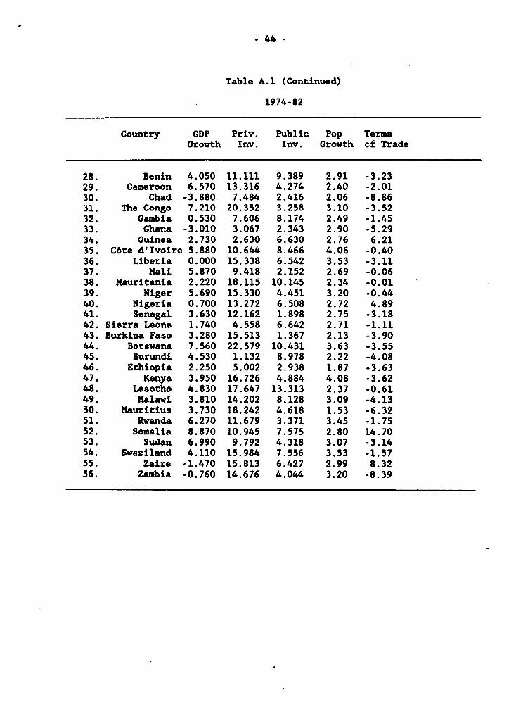
-44-
Table A.1 (Continued)
1974-82
Country GDP Priv. Public Pop TermsGrowth Inv. Inv. Growth cf Trade
28. Benin 4.050 11.111 9.389 2.91 -3.2329. Cameroon 6.570 13.316 4.274 2.40 -2.0130. Chad -3.880 7.484 2.416 2.06 -8.8631. The Congo 7.210 20.352 3.258 3.10 -3.5232. Gambia 0.530 7.606 8.174 2.49 -1.4533. Ghana -3.010 3.067 2.343 2.90 -5.2934. Guinea 2.730 2.630 6.630 2.76 6.2135. C6te dllvoire 5.880 10.644 8.466 4.06 -0.4036. Liberia 0.000 15.338 6.542 3.53 -3.1137. Mali 5.870 9.418 2.152 2.69 -0.0638. Mauritania 2.220 18.115 10.145 2.34 -0.0139. Niger 5.690 15.330 4.451 3.20 -0.4440. Nigeria 0.700 13.272 6.508 2.72 4.8941. Senegal 3.630 12.162 1.898 2.75 -3.1842. Sierra Leone 1.740 4.558 6.642 2.71 -1.1143. Burkina Faso 3.280 15.513 1.367 2.13 -3.9044. Botswana 7.560 22.579 10.431 3.63 -3.5545. Burundi 4.530 1.132 8.978 2.22 -4.0846. Ethiopia 2.250 5.002 2.938 1.87 -3.6347. Kenya 3.950 16.726 4.884 4.08 -3.6248. Lesotho 4.830 17.647 13.313 2.37 -0.6149. Malawi 3.810 14.202 8.128 3.09 -4.1350. Mauritius 3.730 18.242 4.618 1.53 -6.3251. Rwanda 6.270 11.679 3.371 3.45 -1.7552. Somalia 8.870 10.945 7.575 2.80 14.7053. Sudan 6.990 9.792 4.318 3.07 -3.1454. Swaziland 4.110 15.984 7.556 3.53 -1.5755. Zaire -1.470 15.813 6.427 2.99 8.3256. Zambia -0.760 14.676 4.044 3.20 -8.39

- 45 -
Table A.1 (Continued)
1965-73
Country Gov. Gov. Tax Import ExportCons. Growth Effort Tax Tax
1. Benin 12.300 2.700 12.03 18.12 1.722. Cameroon 8.900 5.020 13.18 24.50 6.653. Chad 17.950 5.700 12.81 14.69 4.444. Congo 19.210 7.100 18.80 12.91 2.795. Gabon 16.670 8.800 19.24 18.48 5.616. Gambia 20.900 2.200 13.14 18.89 3.537. Ghana 12.100 -1.600 14.30 15.53 18.478. C6te d'Ivoire 10.100 12.600 20.09 17.46 10.269. Liberia 12.420 3.100 15.54 11.84 0.4010. Mali 18.400 -2.500 9.63 11.15 4.8711. Nigeria 6.650 12.700 7.89 15.69 2.6212. Senegal 17.810 -0.900 16.08 21.61 4.3413. Sierra Leone 14.830 4.000 14.44 20.93 3.8814. Burkina Faso 8.880 7.900 10.98 21.33 2.4315. Botswana 21.140 5.700 14.51 14.48 1.9716. Burundi 9.420 9;600 10.18 20.05 13.2317. Ethiopia 7.980 3.900 9.31 24.96 7.3718. Kenya 15.270 11.000 13.93 .13.84 0.2619. Lesotho 14.040 4-.000 14.40 13.68 2.8620. Madagascar 19.270 2.100 14.74 22.62 5.0321. Malawi 15.500 3.800 11.30 12.01 0.0022. Maxlritius 11.230 2.500 18.00 12.62 3.2823. Rwanda 9.410 2.200 7.93 13.53 13.4424. Somalia 14.440 17.100 12.92 23.83 4.1225. Sudan 22.330 2.700 16.22 36.02 6.5926. Swaziland 14.980 10.000 16.08 10.52 0.0927. Zaire 21.880 5.400 25.30 16.35 24.96

- 46 -
Table A.1 (Continued)
1974-82
Country Gov. Gov. Tax Import ExportCons. Growth Effort Tax Tax
28. Benin 11.830 4.600 17.18 17.00 1.4429. Cameroon 8.140 1.070 15.13 18.99 5.9030. Chad 18.170 -7.000 12.30 12.97 3.6331. The Congo 16.900 4.500 20.46 8.84 0.3532. Gambia 20.940 7.900 13.85 16.06 3.1233. Ghana 16.390 9.400 8.33 12.12 22.1634. Guinea 16.580 6.000 16.54 22.04 22.8335. C6te d'Ivoire 13.970 11.100 21.31 21.60 7.2136. Liberia 12.570 2.700 19.98 10.86 0.1837. Mali 20.020 9.000 12.80 7.73 5.7038. Mauritania 31.700 7.100 19.69 9.05 1.5139. Niger 11.480 2.600 12.96 13.54 3.2540. Nigeria 12.070 7.400 19.08 11.31 0.0341. Senegal 19.700 7.000 17.44 15.04 1.7042. Sierra Leone 11.180 0.000 16.47 17.89 8.1443. Burkina Faso 14.000 10.500 13.91 15.05 2.7044. Botswana 17.640 11.900 23.81 18.80 0.3245. Burundi 12.070 5.000 13.19 15.81 15.8946. Ethiopia 8.590 3.100 14.35 20.25 18.5947. Kenya 20.770 7.000 20.41 11.91 0.4248. Lesotho 23.420 13.500 25.71 13.24 1.4649. Malawi 15.830 7.900 15.18 8.89 0.0050. Mauritius 13.080 6.200 19.82 10.65 5.2251. Rwanda 13.150 13.300 10.24 12.09 15.7152. Somalia 26.260 3.900 15.04 25.79 1.9153. Sudan 15.080 4.800 13.64 26.02 5.4654. Swaziland 16.500 4.200 33.70 17.37 6.0155. Zaire 22.740 0.500 18.94 10.36 14.6756. Zambia 19.550 0.100 23.66 4.95 0.00

- 47 -
Table A.1: (Continued)
1965-73
Country Pers. Corp. Sales Tax InflationTax Tax Tax Growth
1. Benin 2.55 1.90 4.01 10.20 3.502. Cameroon 6.08 2.26 5.46 4.60 5.443. Chad 5.39 2.13 6.26 2.70 4.674. Congo 5.11 3.78 9.24 3.30 5.265. Gabon 3.92 2.93 4.43 8.60 6.186. Gambia 2.66 1.84 1.10 6.20 2.247. Ghana 4.80 5.60 13.49 -4.30 8.438. C6te d'Ivoire 5.10 2.09 12.06 7.90 4.259. Liberia 5.92 6.31 5.07 6.90 1.7010. Mali 2.49 2.53 11.48 3.20 6.7411. Nigeria 0.14 13.83 6.89 23.10 8.6112. Senegal 4.88 1.79 8.17 0.30 3.0113. Sierra Leone 5.34 8.31 4.58 7.50 2.2214. Burkina Faso 10.91 1.34 5.29 4.00 2.4015. Botswana 0.00 0.00 1.05 29.80 5.0016. Burundi 5.18 5.84 8.96 8.90 2.7817. Ethiopia 5.07 4.47 11.40 6.10 1.6818. Kenya 0.74 12.23 7.80 10.70 2.6319. Lesotho 8.51 2.82 1.26 20.60 4.7220. Madagascar 4.61 3.67 12.64 4.10 4.2621. Malawi 8.72 7.79 5.72 12.20 4.1222. Mauritius 8.39 2.73 6.92 -0.50 6.0423. Rwanda 5.15 5.94 6.24 3.80 9.9724. Somalia 5.71 0.02 12.04 6.70 3.o625. Sudan 2.30 6.56 22.42 2.40 7.3526. Swaziland 5.24 4.66 1.18 17.20 4.3127. Zaire 9.04 7.00 4.02 7.10 17.14

- 48 -
Table A.1: (Continued)
19,. -82
Country Pers. Corp. Sales Tax InflationTax Tax Tax Growth
28. Benin 3.18 3.62 3.72 6.60 10.8729. Cameroon 8.77 4.75 8.40 9.80 11.1830. Chad 4.79 2.53 3.58 0.10 7.5531. The Congo 5.82 10.71 7.05 0.80 11.8632. Gambia 3.78 2.21 0.91 9.40 10.4333. Ghana 4.16 4.84 11.43 -9.90 39.4634. Guinea 3.69 14.84 4.09 13.10 4.1735. C6te d'Ivoire 4.95 3.18 9.37 5.20 10.6836. Liberia 14.41 6.09 6.67 3.80 7.0037. Mali 2.96 7.57 9.47 8.10 10.4638. Mauritania 10.29 1.77 5.80 7.80 8.7239. Niger 4.45 10.17 6.72 14.40 11.6440. Nigeria 0.21 48.07 2.13 10.80 11.2041. Senegal 5.36 3.25 7.41 2.70 7.4842. Sierra Leone 7.02 11.11 7.59 -1.00 13.2743. Burkina Faso 5.36 2.00 5.23 5.20 10.1144. Botswana 0.00 0.00 0.57 12.70 12.9045. Burundi 4.94 6.98 11.64 5.10 12.6346. Ethiopia 5.18 8.03 13.00 7.10 3.8647. Kenya 4.73 10.77 15.16 8.80 10.2148. Lesotho 9.78 6.01 0.85 5.10 11.8449. Malawi 7.81 11.72 9.32 7.80 9.8050. Mauritius 9.77 3.46 4.72 6.00 10.3251. Rwanda 2.68 3.74 4.56 8.60 11.0252. Somalia 3.77 0.54 8.33 8.40 12.2953. Sudan 2.58 7.56 14.71 3.30 15.3454. Swaziland 6.84 4.96 1.13 5.80 12.8555. Zaire 13.53 7.00 5.66 -5.70 38.2456. Zambia 9.84 8.20 17.57 1.50 7.40

PPR Working Paper Series
Title Author Date Contact
WPS36 Means and Implications of Social
Security Finance in Developing
Countrles Douglas J. Puffert August 1988 R. Blade-Charest
33754
WPS37 Black Market Premia, Exchange Rate
Unification and Inflation InSub-Saharan Africa Brian Pinto July 1988 R. Blade-Charest
33754
WPS38 Intergovernmental Grants In
Developing Countries Larry Schroeder
WPS39 Fiscal Policy In Low-income Africa Stephen A. O'Connell July 1988 R. Blade-Charest
33754
WPS40 Financial Deregulation and the
Globalization of Capital Markets Eugene L. Versluysen August 1988 R. Blade-Charest
33754
WPS41 Urban Property Taxation in
Developing Countries William Dillinger August 1988 R. Blade-Charest
33754
WPS42 Government Pay and Employment Policies
and Government Performance in
Developing Economies David L. Lindauer August 1988 R. Blade-Cha-est
33754
WPS43 Tax Administration in DevelopingCountries: Strategies and Tools
rf Implementation Tax AdministrationDivision
WPS44 The Size and Growth of Government
Expenditures David L. Lindauer
WPS45- Assigned to WDR
WPS60
WPS61 Student Performance and Schools Costs
in the Philippines' High Schools Emmanuel Jimenez August 1988 T. Hawkins
Vicente Paqueo 33678
Ma. lourdes de Vera
WPS62 Status of Universities in the ArabCountries of the Middle East and
North Africa George 1. Za'rour

PPR Working Paper Series
Title Author Date Contact
WPS63 Does Japan Import Less Than It Should? Kenji Takeuchi July 1988 J. Epps33710
WPS64 Cocoa and Coffee Pricing Policies
In Cote d lvoire Takamasa Akiyama August 1988 0. Gustafson33714
WPS65 Interaction of Infant Mortality and
Fertility and the Effectiveness of
Health and Family Planning Programs Howard Barnum July 1988 S. Ainsworth
31091
WPS66 Slowing the Stork: Better Health for
Women through Family Planning Anthony R. Measham July 1988 A. MancianoRoger W. Rochat 3,3226
WPS67 Price and Tax Policy for Semi-
Subsistence Agriculture in Ethiopia Robart D. Weaver August 1988 0. Gustafson
Sa?d Ali Shire 33714
WPS68 A Comparison of Lamps for Domestic
Lighting In Developing Countries Robert van der Plas
WPS69 Does Local Financing Make Public
Primary Schools More Efficient?
The Philippine Case Emmanual Jimenez August 1988 T. HawkinsVicente Paqueo 33678Ma. Lourdes de Vera
WPS70 Vocational Education and Economic
Environments: Conflict orConvergence? Arvil V. Adams August 1988 T. Hawkins
Antoine Schwartz 33678
WPS71 School Effects on Student Achievement
in Nigeria and Swaziland Marlaine Lockheed August 1988 T. Hawkins
Andre Komenan 33678
WPS72 The Relative Efficiency of Public
Schools in Developing Countries Emmanuel Jimenez August 1988 T. Hawkins
Marlaine Lockheed 33678
Vicente Paqueo
WPS73 Taxation and Output Growth in Africa Jonathan Skinner August 1988 A. BhalIa60359
Top Related