


Languages
Pages
Legal

Asia Pacific Journal of Research ISSN (Print) : 2320-5504
ISSN (Online) : 2347-4793
www.apjor.com Vol: I. Issue XLVII, January 2017
7
SUBSURFACE WATER MODELLING USING SWIM AND FEFLOW
C. P. Kumar1, B. K. Purandara
2, A. G. Chachadi
3
1Scientist ‘G’, National Institute of Hydrology, Roorkee – 247667 (Uttarakhand), India
2Scientist ‘F’, Hard Rock Regional Centre, NIH, Belagavi – 590001 (Karnataka), India
3Professor & Head, Department of Earth Science, Goa University, Goa – 403206, India
ABSTRACT
Mathematical models provide a scientific and predictive tool for determining appropriate solutions to water allocation, surface water
– groundwater interaction, landscape management or impact of new development scenarios. However, if the modelling studies are not
well designed from the outset, or the model doesn’t adequately represent the natural system being modelled, the modelling effort may
be largely wasted, or decisions may be based on flawed model results, and long term adverse consequences may result. This article
presents case studies on modelling of soil moisture movement (unsaturated flow) using SWIM and modelling of seawater intrusion
(density-dependent groundwater flow) using FEFLOW.
Keywords: Unsaturated flow, Groundwater, Modelling, SWIM, FEFLOW
1. Introduction
Groundwater development has shown phenomenal progress in our country during past few decades. There has been a vast
improvement in the perception, outlook and significance of groundwater resource. Groundwater is a dynamic system. It is dynamic in
the sense that the state of any hydrological system is changing with time, and in the sense that we are continually developing new
scientific techniques to evaluate these systems.
The total annual replenishable groundwater resource of India is around 431 BCM. Inspite of the national scenario on the availability of
groundwater being favourable, there are many areas in the country facing scarcity of water. This is because of the unplanned
groundwater development resulting in fall of water levels, failure of wells, and salinity ingress in coastal areas. The development and
over-exploitation of groundwater resources in certain parts of the country have raised the concern and need for judicious and scientific
resource management and conservation.
A complexity of factors - hydrogeological, hydrological and climatological, control the groundwater occurrence and movement. The
precise assessment of recharge and discharge is rather difficult, as no techniques are currently available for their direct measurements.
Hence, the methods employed for groundwater resource estimation are all indirect. Groundwater being a dynamic and replenishable
resource is generally estimated based on the component of annual recharge, which could be subjected to development by means of
suitable groundwater structures.
Mathematical models are tools, which are frequently used in studying groundwater systems. In general, mathematical models are used
to simulate (or to predict) the groundwater flow. Predictive simulations must be viewed as estimates, dependent upon the quality and

Asia Pacific Journal of Research ISSN (Print) : 2320-5504
ISSN (Online) : 2347-4793
www.apjor.com Vol: I. Issue XLVII, January 2017
8
uncertainty of the input data. Model conceptualization is the process in which data describing field conditions are assembled in a
systematic way to describe groundwater flow processes at a site. The model conceptualization aids in determining the modelling
approach and which model software to use.
This article presents two case studies – (a) modelling of soil moisture movement using SWIM (Soil Water Infiltration and Movement)
and (b) modelling of seawater intrusion using FEFLOW (Finite Element FLOW).
2. SWIM Case Study - Modelling of Soil Moisture Movement
The objective of the study was to simulate the movement of soil moisture in Barchi watershed (sub-basin of Kali river in North Kanara
district of Karnataka) using the SWIM model. The SWIM (Soil Water Infiltration and Movement) is a software package developed by
Division of Soils, CSIRO, Australia (Verburg et al., 1996) for simulating infiltration, evapotranspiration, and redistribution. It has
been selected for the present study in view of its simplicity, ease of use, graphical display of intermittent results, and use of input
parameters (soil moisture characteristics) which can be directly measured in the field/laboratory.
2.1 Study Area
The Barchi watershed upstream of Barchi is located in the leeward side of western ghat and is a sub-basin of Kali river. It lies in
Haliyala taluk of Karwar (North Kanara) district in Karnataka. The location and drainage system of Barchi watershed is shown in
Figure 1.
The Barchinala stream originates from Thavargatti in Belgaum district at an altitude of about 734 m, 20 km north of Dandeli and
flows through North Kanara district of Karnataka State. The catchment is relatively short in width and river flows in a southerly
direction and joins the main Barchi river near the gauging site. The geographical area covered by Barchi watershed is 21.126 km2. The
watershed lies between 74o36’ and 74
o39’ East longitudes, and 15
o18’ and 15
o24’ North latitudes.
High land region consists of dissection of high hills and ridges forming part of the foot hills of western ghats. It consists of steep hills
and valleys intercepted with thick forest. The slopes of the ghats are covered with dense deciduous forest. Forest cover occupies
around 76% of the study area. The watershed is mainly covered with Bamboo, Teak and mixed plantations. The brownish and fine-
grained soils are the principal types of soils found in the area. The following land uses were observed in the watershed:
1. Bamboo plantation = 04 %
2. Teak plantation = 40 %
3. Mixed forest = 32 %
4. Agricultural land = 24 %
Figure 1: Drainage System of Barchi Watershed

Asia Pacific Journal of Research ISSN (Print) : 2320-5504
ISSN (Online) : 2347-4793
www.apjor.com Vol: I. Issue XLVII, January 2017
9
The stream gauging site is located at an elevation of 480 m, where the nala crosses Dandeli-Thavargatti road, about 5 km from
Dandeli. The stream is a 4th
order stream and joins main Barchi river downstream of the gauging site. A full fledged meteorological
station, maintained by Water Resources Development Organisation (WRDO), Karnataka, is located near the gauging site.
The Barchi raingauge station is located at 15o18’ N and 74
o37’ E. Average annual rainfall for the watershed is 1500 mm, majority of
which occurs during the south-west monsoon period. Depth to water table varies between 4 to 12 metres during pre- and post-
monsoon periods. The yield of borewells in the study area is found to vary between 120 gallons per hour to 1170 gallons per hour.
2.2 Methodology
The study involves modelling of soil moisture movement in Barchi watershed using the SWIM model. The following steps were
undertaken for the study.
Field investigations: Measurement of saturated hydraulic conductivity at 8 locations using Guelph Permeameter and soil
sampling.
Laboratory investigations: Determination of saturated moisture content, and soil moisture retention characteristics using the
Pressure Plate Apparatus.
Modelling of soil moisture movement using the SWIM model: Daily rainfall and evaporation data of Barchi for the period
1996-97 to 1999-2000 were used for the study. Water balance components like runoff, evapotranspiration and drainage
(recharge to groundwater from rainfall) were determined through SWIM.
SWIM is an acronym that stands for Soil Water Infiltration and Movement. It is a software package developed within the CSIRO
Division of Soils for simulating infiltration, evapotranspiration, and redistribution. The first version (SWIMv1) was published in 1990
(Ross2, 1990). Version 2 of the model (identified as SWIMv2.0), which combines water movement with transient solute transport and
which accommodates a variety of soil property descriptions and more flexible boundary conditions, was completed in 1992.
SWIMv2 is based on a numerical solution of the Richards’ equation (1) and the advection-dispersion equation (2), as given below.
The model deals with a one-dimensional soil profile.
t x
d
dp
p
x
dz
dxS
…(1)
with
o
o
o
o
p
p
1
1
sinh
where,
= volumetric water content (cm3/cm
3);
t = time (h);
x = distance into the soil (cm soil);
K = hydraulic conductivity (cm2 water/cm soil/h);
= matric potential (cm);
z = gravitational potential (cm);
S = source (or sink, if negative) strength (cm3 water/cm
3 soil/h); and
o and 1 = shifting and scaling parameters, respectively.
Solute movement is based on the following solute transport equation

Asia Pacific Journal of Research ISSN (Print) : 2320-5504
ISSN (Online) : 2347-4793
www.apjor.com Vol: I. Issue XLVII, January 2017
10
c
t
s
t xD
c
x
qc
x
…(2)
where,
c = solute concentration in solution (mol or g solutes/cm3
water);
s = adsorbed concentration (mol/g soil or g/g soil);
= soil bulk density (g/cm3);
t = time (h);
x = depth (cm);
= water content (cm3/cm
3);
q = water flux density (cm/h);
D = combined dispersion and diffusion coefficient (cm2/h); and
= source/sink term (mol/cm3/h or g/cm
3/h).
The SWIM can be used to simulate runoff, infiltration, redistribution, solute transport and redistribution of solutes, plant uptake and
transpiration, soil evaporation, deep drainage and leaching. The physical system and the associated flows addressed by the model are
shown schematically in Figure 2. Soil water and solute transport properties, initial conditions, and time dependent boundary conditions
(e.g., precipitation, evaporative demand, solute input) need to be supplied by the user in order to run the model. The overall purpose of
the model is to address issues relating to the soil water and solute balance. As such, it is a research tool that can be integrated in
laboratory and field studies concerned with soil water and solute transport.
Figure 2: Components of the Soil Water and Solute Balances Addressed by SWIMv 2.1
To model the retention and movement of water and chemicals in the unsaturated zone, it is necessary to know the relationships
between soil water pressure (h), water content () and hydraulic conductivity (K). It is often convenient to represent these functions by
means of relatively simple parametric expressions. The problem of characterizing the soil hydraulic properties then reduces to
estimating parameters of the appropriate constitutive model.
The measurements of (h) from soil cores (obtained through pressure plate apparatus) can be fitted to the desired soil water retention
model. Once the retention function is estimated, the hydraulic conductivity relation, K(h), can be evaluated if the saturated hydraulic
conductivity, Ks, is known. In the present study, parameters of van Genuchten model were derived for soil moisture retention and
hydraulic conductivity functions. For the van Genuchten3 model (1980), the water retention function is given by

Asia Pacific Journal of Research ISSN (Print) : 2320-5504
ISSN (Online) : 2347-4793
www.apjor.com Vol: I. Issue XLVII, January 2017
11
Se = ( - r)/(s - r) = [ 1 + (v h )n ]
-m for h 0
= 1 for h 0
…(3)
and the hydraulic conductivity function is described by
K = Ks Se1/2
[ 1 – (1 – Se1/m
)m
]2 …(4)
where, Se is effective saturation; r is residual water content; s is saturated water content; v and n are van Genuchten model
parameters; m = 1 – 1/n.
Modelling of soil moisture movement in Barchi watershed was done using SWIM. The model was simulated for 1461 days (1 May
1996 to 30 April 2000). One vegetation type (teak, covered in most parts of the watershed) was considered for the study. Exponential
root growth with depth and linear interpolation with time was assumed. The following vegetation parameters were adopted for the
simulations:
Root radius (rad) = 0.5 cm
Root conductance (groot) = 4.0 * 10-7
Minimum xylem potential (psimin) = -15,000 cm
Root depth constant (xc) = 150 cm
Maximum root length density (rldmax) = 4 cm/cm3
2.3 Results and Discussion
Soil moisture retention characteristics were determined in the laboratory using the Pressure Plate Apparatus. The experimental soil
moisture retention data were fitted to the van Genuchten3 model (1980). Residual moisture content (r) was assumed to be equivalent
to moisture retained corresponding to 15 bar pressure. The parameters of soil moisture retention function and hydraulic conductivity
function were obtained through non-linear regression analysis. Tables 1 and 2 present the van Genuchten parameters and n
(equations 3 and 4) for upper and lower soil layers in Barchi watershed. Average values of these parameters were also determined
through non-linear regression analysis and used in modelling of soil moisture movement through SWIM.
Table 1: van Genuchten Parameters for Upper Soil Layer
Station Ks
(cm/hour) r s
van Genuchten Parameters Proportion of
Variance
Explained (%) n
1 0.58 0.08 0.37 0.0073 1.434 80.78
2 0.57 0.14 0.37 0.0023 1.509 74.08
3 0.60 0.09 0.38 0.0021 1.465 79.07
4 0.18 0.30 0.53 0.0067 1.523 92.00
5 0.20 0.28 0.53 0.0129 1.373 80.66
6 0.18 0.28 0.53 0.0235 1.300 64.09
7 0.24 0.25 0.52 0.0020 1.580 84.07
8 0.16 0.30 0.54 0.0019 1.552 91.51
Average 0.339 0.215 0.471 0.0047 1.4385 24.43

Asia Pacific Journal of Research ISSN (Print) : 2320-5504
ISSN (Online) : 2347-4793
www.apjor.com Vol: I. Issue XLVII, January 2017
12
Table 2: van Genuchten Parameters for Lower Soil Layer
Station Ks
(cm/hour) r s
van Genuchten Parameters Proportion of Variance Explained (%)
n
1 1.66 0.11 0.38 0.0148 1.563 97.04
2 0.60 0.09 0.32 0.0045 1.760 99.52
3 0.007 0.06 0.43 0.0154 1.358 87.12
4 0.58 0.14 0.41 0.0134 1.310 81.71
5 0.58 0.16 0.43 0.0070 1.444 91.68
6 0.18 0.28 0.53 0.0235 1.300 64.09
7 0.59 0.13 0.31 0.0120 1.596 95.35
8 0.60 0.20 0.45 0.0123 1.688 91.97
Average 0.648 0.121 0.394 0.0095 1.4212 58.31
Based upon the available information, two distinct soil layers were identified (0-45 cm and 45-150 cm). Saturated hydraulic
conductivity was measured at 8 locations in the study area by using Guelph Permeameter (locations are shown in Figure 1). The
average saturated hydraulic conductivity values for the upper layer (0-45 cm) and lower layer (45-150 cm) were found to be 0.339
cm/hour and 0.648 cm/hour respectively.
2.3.1 Model Conceptualization
The profile is 150 cm deep with surface at 0 cm and bottom boundary condition applying at 150 cm. Vapour conductivity is not taken
into account, nor is the effect of osmotic potential. There are two hydraulic property sets (for upper and lower soil layers) that are
applied to 31 depth nodes of the 150 cm deep profile. Hysteresis is not taken into account.
Initially, there is no water ponded on the surface. Runoff is governed by a simple power law function and a surface conductance
function. No bypass flow was included. A matric potential gradient of 0, i.e. “unit gradient”, has been applied as bottom boundary
condition throughout the simulation. Cumulative rainfall and evaporation records (daily) for the period 1996-97 to 1999-2000 were
given in the input file for determination of water balance components (runoff, evapotranspiration and drainage).
2.3.2 Simulation of Water Balance Components
The model parameters (soil moisture characteristics) were actually measured in the field and laboratory. Therefore, the model does not
require any calibration as such. The model was validated by comparing the observed and simulated runoff. However, the observed
runoff values were suspected to be erroneous in view of inaccurate positioning of zero of gauge.
Self-recording raingauge data (hourly rainfall values) were not available for the watershed. Therefore, daily rainfall values were used.
However, with the available input data and parameters, the model was found to underestimate the runoff values. It happened because
daily rainfall data generated low rainfall intensities (distributed over 24 hours) with most of the rainfall infiltrating into the ground and
contributing less runoff. Therefore, daily rainfall values were equally distributed to 4 hours for the periods exceeding 20 mm rainfall
in a day. This made a better agreement between the observed and simulated runoff and therefore validated the model. The distribution
of daily rainfall into 4 hours was decided on the basis of trial simulations by testing varying divisions with part of actual data. The
resulting water balance components for the simulation period have been presented in Table 3.

Asia Pacific Journal of Research ISSN (Print) : 2320-5504
ISSN (Online) : 2347-4793
www.apjor.com Vol: I. Issue XLVII, January 2017
13
Table 3: Water Balance Components for the Barchi Watershed
Year Rainfall
(mm)
Infiltration
(mm)
Drainage
(mm)
ET
(mm)
Runoff
(mm)
Runoff Coefficient
(%)
Recharge
Coefficient
(%)
1996-1997 1345.85 1083.37 514.46 519.52 262.48 19.50 38.22
1997-1998 1765.25 1195.05 698.63 500.43 570.20 32.30 39.58
1998-1999 1241.30 1087.46 579.55 507.92 153.84 12.39 46.69
1999-2000 1886.80 1278.18 784.90 493.28 608.62 32.26 41.60
Total 6239.20 4644.06 2577.54 2021.15 1595.14 24.11 41.52
The yearly rainfall varied between 1241 mm to 1887 mm during the period under study. It can be observed from Table 3 that the
drainage (recharge from rainfall) varies from 38% to 47% with the average value being 42%. The runoff coefficient was found to vary
between 12% (low rainfall year) to 32% (high rainfall year) with the average value being 24%. Runoff coefficient was found to be
lower in low rainfall years (1996-97 and 1998-99). It can be attributed to low rainfall intensities enabling more infiltration and lesser
runoff. Antecedent moisture conditions also play an important role in the runoff generation process. Simulation of variable infiltration
suggests that it has relatively little effect on evapotranspiration, but considerable effect on point drainage.
2.4 Conclusion for SWIM Case Study
Application of SWIM model is one of the simplest techniques, which is well suited for unsaturated zone. SWIM is a software package
for simulating water infiltration and movement in soils. Water is added as precipitation and removed by runoff, drainage, evaporation
from the soil surface and transpiration by vegetation. The simulator assumes that conditions can be treated as horizontally uniform,
flow is described by the Richards equation and soil hydraulic properties can be described by simple functions. While this is adequate
for many purposes, there are situations where it is not and the simulation results should never be applied uncritically.
Water balance components like runoff, evapotranspiration and drainage were determined through SWIM for the period 1996-97 to
1999-2000. The ground water recharge was found to vary between 38% to 47% of rainfall while the runoff coefficient varied between
12% (low rainfall year) to 32% (high rainfall year) for the study period. Variable infiltration was observed to have relatively little
effect on evapotranspiration, but considerable effect on drainage.
The SWIM model demonstrated the possibility of predicting water balance components of the unsaturated zone, but only with careful
selection of input parameters. It would appear that when actual observed data is not available, it would be difficult to rely upon
numerical models alone.
3. FEFLOW Case Study - Modelling of Seawater Intrusion
Coastal tracts of Goa are rapidly being transformed into settlement areas. The poor water supply facilities have encouraged people to
have their own source of water by digging or boring a well. During the last decade, there have been large-scale withdrawals of
groundwater by builders, hotels and other tourist establishments. Though the seawater intrusion has not yet assumed serious
magnitude, but in the coming years it may turn to be a major problem if corrective measures are not initiated at this stage. It is
necessary to understand how fresh and salt water move under various realistic pumping and recharge scenarios. Objectives of this
study include simulation of seawater intrusion in a part of the coastal area in Bardez taluk of North Goa, evaluation of the impact on
seawater intrusion due to various groundwater pumping scenarios and sensitivity analysis to find the most sensitive parameters
affecting the simulation.
3.1 Study Area
The study area lies in Bardez taluka of North Goa within the watersheds of Baga river and Nerul creek (around 74 km2) and covered
by Survey of India toposheets number 48E/10, 48E/14 and 48E/15 on 1:50,000 scale. It is bound by rivers Chapora and Mandovi in
north and south directions respectively, besides Arabian sea in the west and encompasses coastal tract from Fort Aguada in the south
to Fort Chapora in the north (15 km). The soils are predominantly of lateritic nature. However, the coastal areas are made up of
alluvial soils composed of loamy mixed sand and loamy sands. Around 30 km2 area close to the coast (15 km along the coast and 2 km
wide) is more prone to seawater intrusion. Layout maps of North Goa and the study area are given in figures 3 and 4 respectively.

Asia Pacific Journal of Research ISSN (Print) : 2320-5504
ISSN (Online) : 2347-4793
www.apjor.com Vol: I. Issue XLVII, January 2017
14
Figure 3: Location Map of Study Area in Goa
3.2 Laboratory and Field Investigations
Twenty observation wells were identified in the study area (as indicated in figure 4). Monthly groundwater level data was measured in
observation wells (September 2004 to August 2005) and groundwater samples were collected in September, November 2004, January,
March, April, May 2005. Salinity for collected groundwater samples was measured in the laboratory. Based upon the bi-monthly
measurements of salinity, groundwater quality in all the observation wells was found to be reasonably fresh, both in pre- and post-
monsoon periods. It can be attributed to the fact that the transition zone of fresh water-saline water lies below the shallow open wells,
as evidenced by vertical electrical soundings.
Apparent electrical resistivity (ohm-m) was measured in four profiles along the Bardez coast (Anjuna, Baga, Calangute, Candolim) at
18 locations upto 525 metres from the coast (Table 4). The inter-electrode separation was kept at 10 meter, that is, the resistivity
values measured are at 10 m depth plane. The seawater mixed zone is witnessed along Anjuna (12 to 45 ohm-m) and Baga beach (4 to
46 ohm-m) sections along the low lying sandy alluvial areas. Very close to the sea, relatively higher apparent resistivity values are due
to dry sand dunes. However, along Calangute (75 to 900 ohm-m) and Candolim (142 to 700 ohm-m) beaches, there is no indication of
seawater mixing at 10 m depth, as all values are higher.
Figure 4: Layout Map of the Study Area

Asia Pacific Journal of Research ISSN (Print) : 2320-5504
ISSN (Online) : 2347-4793
www.apjor.com Vol: I. Issue XLVII, January 2017
15
Seven vertical electrical soundings were carried out at monitoring well sites 1, 3, 6, 7, 8, 15 and 17 (Table 5). These were restricted to
a depth of 20 m to know any change in the quality of water vis-à-vis seawater intrusion (3 m to 20 m with 1 m interval). As seen from
the apparent resistivity values, well numbers 6, 7 and 8 show low values of resistivity (2 to 33 ohm-m) below about 12 m depth,
indicating the presence of seawater or mixed zone below this depth. However, at other sites, there is no indication of the seawater
mixing upto 20 m depth. It is noted here that wells located in low lying sandy alluvial areas show seawater mixing than the wells
located in laterites at higher altitudes. In both laterite and alluvial soils, the wells are built well above the salt water – fresh water
interface and hence no change in water quality was found in summer also.
Table 4: Apparent Electrical Resistivity Values (ohm-m) in Four Profiles along the Bardez Coast
S. No. Distance from Coast (m) P1 P2 P3 P4
Anjuna Baga Calangute Candolim
1 15 30 70 150 700
2 45 40 46 820 555
3 75 45 35 612 142
4 105 32 25 360 421
5 135 26 28 110 281
6 165 24 22 75 153
7 195 20 30 125 184
8 225 15 32 242 255
9 255 14 24 410 431
10 285 12 20 623 236
11 315 13 31 531 165
12 345 13 32 415 242
13 375 14 20 324 281
14 405 16 30 470 641
15 435 20 20 684 531
16 465 21 10 650 426
17 495 24 5 835 186
18 525 18 4 900 200
Table 5: Apparent Electrical Resistivity Values (ohm-m) at Observation Well Points in the Study Area
AB/2
(m)
Apparent Electrical Resistivity Values (ohm-m)
at Monitoring Well Numbers
1 3 6 7 8 15 17
3 410 448 80 102 231 1988 333
4 436 446 65 84 277 665 356
5 467 521 63 72 202 900 373
6 505 595 68 62 180 256 393
7 536 613 82 58 138 850 383
8 541 521 74 51 120 156 381
9 533 482 47 45 102 780 381
10 544 389 62 42 62 194 327
11 528 339 56 40 61 125 339
12 539 314 23 25 45 128 314
13 581 264 24 22 41 158 290
14 582 245 19 18 31 165 276
15 563 246 20 16 32 164 246
16 561 240 21 17 33 215 240
17 543 226 13 15 25 265 226
18 609 233 16 12 10 315 203
19 566 215 12 18 3 452 226
20 520 214 9 17 2 351 202

Asia Pacific Journal of Research ISSN (Print) : 2320-5504
ISSN (Online) : 2347-4793
www.apjor.com Vol: I. Issue XLVII, January 2017
16
3.3 Finite Element Simulation Model
For this study, a finite-element model (FEFLOW) was selected for model simulations. The FEFLOW is an interactive finite element
simulation system (Version 5.1) for three-dimensional (3D) or two-dimensional (2D), i.e. horizontal (aquifer-averaged), vertical or
axi-symmetric, transient or steady-state, fluid density- coupled or linear, flow and mass, flow and heat or completely coupled
thermohaline transport processes in subsurface water resources (groundwater systems). The package is fully graphics-based and
interactive. Pre-, main- and post-processing are integrated. There is a data interface to GIS (Geographic Information System) and a
programming interface. The implemented numerical features allow the solution of large problems.
3.3.1 Model Setup and Simulation Results
The aquifer domain of the study area (74 km2) was discretized using 6 nodal triangular prism elements with 52,656 mesh elements and
32,053 mesh nodes. The vertical discretization corresponds to 7 slices and 6 layers. The top slice was defined as free and movable
(water table). Geological profile in low lying area (ground elevation 0 – 20 m above mean sea level) was assigned as 15 – 30 m deep
sandy soil (upto 10 – 15 m below mean sea level) underlain by 1 – 2 m clay layer and then basement rocks (phyllite, graywacke, schist
etc). Geological profile in plateau area (ground elevation 20 – 80 m above mean sea level) was assigned as 0 - 75 m deep laterite (upto
0 – 10 m below mean sea level) underlain by 2 – 5 m clay layer and then basement rocks. The boundary conditions for the flow
simulation are as follows:
A coastal head boundary along the coastal zone (western boundary) at the top and bottom slices of the aquifer; FEFLOW
uses head (h) instead of pressure with h = (ew / es) Z, where ew and es represent ambient and seawater densities respectively
and Z is the depth below sea level. The head was calculated in each constant-head boundary node.
No flow boundaries are specified in the eastern boundary and right part of the northern boundary, where it forms the
watershed boundary of Baga and Nerul rivers.
Southern boundary (Mandovi river) and left part of the northern boundary (Chapora river) are described by third-kind
(Cauchy) boundary condition, Transfer. Internal flow boundaries (Baga river and Nerul river) are also described by Transfer
boundary condition.
The boundary conditions and initial concentration for the transient state solute transport are dependent on the flow simulation results.
For this model, solute transport concentrations are expressed in terms of total dissolved solids (TDS). A concentration of 35,425 mg/l
(seawater TDS) is used along the coastal zone where simulated inflow from ocean occurs (mass boundary of 1st kind). The initial
concentration of the groundwater was set to 0 mg/l.
The aquifer geometry was adopted, as defined in previous studies. Reference zero elevation was assumed at 50 m below mean sea
level. Only few measured hydrodynamic data are available and incorporated in the model. Four values of hydraulic conductivity
ranging from 0.381x10⁻⁴
to 3.657x10⁻⁴
m/s were measured through pumping tests. Data regionalization for hydraulic conductivity over
the study area has been carried out using Akima inter/extrapolation. No measurement of dispersivity has been made, this parameter
was therefore estimated by trial and error using prior information from similar cases. Molecular diffusion was assumed as 1.00x10⁻⁹
m2/s. Initial head data have been measured in 20 observation wells. Data regionalization for hydraulic heads over the study area has
been carried out using Akima inter/extrapolation.
The transient state simulation of the solute transport was carried out using automatic time step control via predictor-corrector schemes,
with initial time step length as 0.001 day and final time as 3650 days (10 years) to reach steady state conditions. Calibration objective
for the mass transport was focused mainly at observation wells near Anjuna and Baga beaches and Baga river where resistivity survey
has indicated the presence of brackish water.
Mean annual rainfall is estimated to be 2714 mm, based upon daily rainfall data of Panaji for 20 years (1984 to 2003). Rainfall
recharge values for laterite and west coast were adopted as 7% and 10% respectively, as recommended by “Groundwater Resource
Estimation Methodology - 1997”. Annual groundwater draft for the study area was worked out by using the reported density of wells
as 25 wells per km2 and average annual groundwater draft per structure as 0.65 ha-m. Porosity for sandy alluvium, laterite and clay
were assumed to be 0.32, 0.21 and 0.42 respectively. Specific yield for sandy alluvium, laterite and clay were assumed to be 0.16,
0.025 and 0.03 respectively.

Asia Pacific Journal of Research ISSN (Print) : 2320-5504
ISSN (Online) : 2347-4793
www.apjor.com Vol: I. Issue XLVII, January 2017
17
Figure 5: Three-dimensional Plot for Mass Distribution
Longitudinal and transverse dispersivity were modified uniformly by trial and error in order to match the measured salinity values
from the observation wells. Several runs were carried out to approach the solution. Final calibrated longitudinal and transverse
dispersivity are 50 m and 5 m respectively. The calibration process shows that the mass transport model is sensitive to the dispersivity
values.
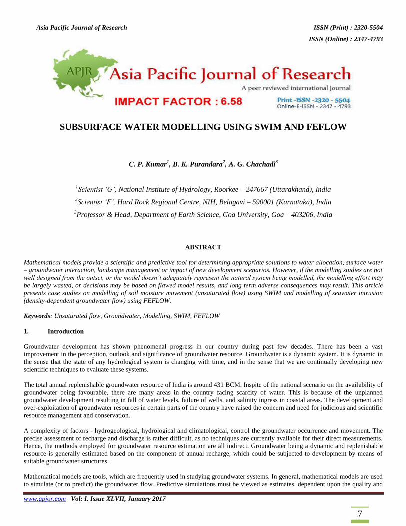
Three-dimensional plot for mass distribution has been presented in figure 5. It indicates 3 peaks where salinity near the coast exceeds
6000 mg/l. Along these three sections, the salinity of groundwater was found to be greater than 500 mg/l upto 300 m inland, the
maximum (near the coast) being 9400 mg/l, 9600 mg/l and 6800 mg/l respectively. The computed salinity in the aquifer show a sharp
decrease of salinity from the coast towards inland. As an example, for the middle section, the salinity varies from 9,600 mg/l to 500
mg/l from the coastal front to a distance 300 m, as shown in figure 6. The model was not fully calibrated because of uncertainties in
the hydrodynamic flow and mass transport data used. However, the results show that the density dependent 3D model is reasonable.
Asia Pacific Journal of Research ISSN (Print) : 2320-5504
ISSN (Online) : 2347-4793
www.apjor.com Vol: I. Issue XLVII, January 2017
18
Figure 6: Mass Distribution along a Section
3.4 Conclusion for FEFLOW Case Study
The above results indicate that presently, seawater intrusion is confined only upto 300 m from the coast under normal rainfall
conditions and present draft pattern. It may be slightly more for low rainfall years. However, seawater intrusion may further advance
inland if withdrawals of groundwater by builders, hotels and other tourist establishments continue to increase in the coming years.
Therefore, corrective measures with proper planning and management of groundwater resources in the area need to be initiated at this
stage so that it may not turn to be a major water quality problem in the coming times. This study will guide in making management
decisions to monitor and control seawater intrusion and planning of groundwater development in the area.
References
1. Chachadi, A.G. (2000). Strategies for Water Resources Management in the Coastal Zones of Goa. Coastal Zone
Management, S.D.M.C.E.T, Dharwad & IGCP-367, Special Publication, Volume No. 2, pp. 165-168.
2. Chachadi, A.G. and C. Joaquim S. John (2000). Geoelectrical Studies in Ascertaining Fresh-Water Zones in Coastal Goa.
Coastal Zone Management, S.D.M.C.E.T, Dharwad & IGCP-367, Special Publication, Volume No. 2, pp. 169-172.
3. Chachadi, A. G., J. P. Lobo-Ferreira, Ligia Noronha and B. S. Choudri (2002). Assessing the Impact of Sea-Level Rise on
Salt Water Intrusion in Coastal Aquifers using GALDIT Model, Coastin – November 2002, TERI, pp. 27-32.
Asia Pacific Journal of Research ISSN (Print) : 2320-5504
ISSN (Online) : 2347-4793
www.apjor.com Vol: I. Issue XLVII, January 2017
19
4. Cheng, Alexander H.-D. (2003). Groundwater, Saltwater Intrusion in. Encyclopedia of Water Science, Marcel Dekker, Inc.,
pp. 404-406.
5. COASTIN (2001). GIS and Mathematical Modelling for the Assessment of Groundwater Vulnerability to Pollution:
Application to an India Case – Study Area in Goa. 2nd
Year Report, April 2001, 69 p.
6. Diersch, H.-J. G. (2002). FEFLOW Reference Manual, Finite Element Subsurface Flow & Transport Simulation System.
WASY Institute for Water Resource Planning and Systems Research Ltd., Berlin, 278 p.
7. FEFLOW (Finite Element Subsurface Flow & Transport Simulation System) Demonstration Exercise, WASY Institute for
Water Resource Planning and Systems Research Ltd., Berlin, 2004, 48 p.
8. FEFLOW 5.1 (Finite Element Subsurface Flow & Transport Simulation System) User’s Manual, WASY Institute for Water
Resource Planning and Systems Research Ltd., Berlin, 2004, 168 p.
9. Goa University (2000). Aquifer Testing, Observation Well Networking, Electrical Profiling and Groundwater Draft
Estimation, Baga Watershed, Bardez, Goa. Department of Geology, Goa University, Goa, 46 p.
10. Groundwater Resource Estimation Methodology - 1997. Report of the Groundwater Resource Estimation Committee,
Ministry of Water Resources, Government of India, New Delhi, June 1997.
11. Kumar, C. P. and B. K. Purandara (2003). Modelling of Soil Moisture Movement in a Watershed using SWIM. Journal of
The Institution of Engineers (India), Agricultural Engineering Division, Volume 84, December 2003, pp. 47-51.
12. Kumar, C. P., A. G. Chachadi, B. K. Purandara, Sudhir Kumar and Raju Juyal (2007). Modelling of Seawater Intrusion in
Coastal Area of North Goa. Water Digest, Vol. II, Issue 3, September-October 2007, pp. 80-83.
13. Lobo-Ferreira, J. P., Maria C. Cunha, A. G. Chachadi, Kai Nagel, Catarina Diamantino and Manuel M. Oliveira (2003).
Application of Optimization Models for Satisfaction of Water Resource Demand of Tourist Infrastructure. In. Coastal
Tourism, Environment, and Sustainable Local Development (Ed. Noronha et al.), Chapter 14, pp. 305-320.
14. Purandara, B. K. and C. P. Kumar (2000). Simulation of Soil Moisture Movement in a Forested Watershed. ICIWRM-2000,
Proceedings of International Conference on Integrated Water Resources Management for Sustainable Development, 19-21
December, 2000, New Delhi, India, pp. 833-839.
15. Ross, Peter J. (1990). SWIM - A Simulation Model for Soil Water Infiltration and Movement. Reference Manual to
SWIMv1, CSIRO Division of Soils, Australia, 1990.
16. Verburg Kirsten, Peter J. Ross and Keith L. Bristow (1996). SWIMv2.1 User Manual. CSIRO Division of Soils, Australia,
Divisional Report No. 130, 1996.
17. van Genuchten, M. Th. (1980). A Closed-form Equation for Predicting the Hydraulic Conductivity of Unsaturated Soils. Soil
Sci. Soc. Am. J., Volume 44, 1980, pp. 892-898.
Top Related