


Languages
Pages
Legal


Structural Dynamics
Lecture 10
Outline of Lecture 10
� Continuous Systems (cont.).
� Dynamic Modelling of Structures.
� SDOF Model.
� 2DOF Model.
� Introduction to the Finite Element Method.
11
� Introduction to the Finite Element Method.
� Equations of Motion of a Plane Bernoulli-Euler Beam Element.
� Global Equations of Motion.

Structural Dynamics
Lecture 10
� Continuous Systems (cont.)
� Dynamic Modelling of Structures
Dynamic modelling means the reduction of an infinite many degrees-of-freedom system to a system with finite many degrees of freedom.
The partial differential equation with given boundary values of the problem
22
The partial differential equation with given boundary values of the problem is replaced by an ordinary matrix differential equation:
� : Vector of selected degrees-of-freedom vector, .
� : Mass matrix, .
� : Damping matrix, .
� : Stiffness matrix, .
� : Dynamic load vector, .

Structural Dynamics
Lecture 10
The modelling involves the specification of , , , , , so the discrete system describes the continuous system “at best”.
This is done by interpolating the continuous displacement field of the structure by a discrete number of appropriate shape functions with a corresponding number of amplitude functions of time, , which represent the selected degrees of freedom. The optimal behaviour of
follows from analytical dynamics. is determined by Rayleigh or
33
follows from analytical dynamics. is determined by Rayleigh or Caughey damping, presuming that a given number of modal damping ratios are measured or prescribed.
The method will be illustrated with respect to the wind turbine blade shown on Fig. 1, which is modelled as a cantilever Bernoulli-Euler beam.

Structural Dynamics
Lecture 10
44

Structural Dynamics
Lecture 10
The boundary value problem of a rotating blade reads, cf. Lecture 9Eq. (39) and Lecture 9, Fig. 9b:
55
� : Rotational speed of blade [ ].
� : Mean wind velocity [ ].
� : Mass per unit length, [ ].
� : Bending stiffness around the -axis, [ ].
� : Axial force due to centrifugal acceleration, [ ]. .
� : Displacement in the -direction (out-of-rotor plane), [ ].
� : Dynamic load per unit length in the -direction, [ ].

Structural Dynamics
Lecture 10
Axial force (centrifugal force):
Interpolation of the displacement field relative to the rigid body motion of the blade:
66

Structural Dynamics
Lecture 10
� : Shape function (interpolation function).
77
� : Shape function (interpolation function).
� : Generalized coordinates (degrees of freedom).
The shape functions must be linearly independent, and must fulfill the
geometric boundary conditions at the hub:

Structural Dynamics
Lecture 10
The shape functions need not fulfill the mechanical boundary conditions at
( ). It is favourable that one or both of these boundary conditions are fulfilled. This makes the undamped eigenmodes
the best choice for the shape functions.
Kinetic energy of the continuous system:
88
Potential energy of the continuous system:

Structural Dynamics
Lecture 10
Kinetic and potential energy of the discrete system:
99
Generally, the consistent mass matrix is not diagonal.
: Consistent mass matrix.

Structural Dynamics
Lecture 10
1010

Structural Dynamics
Lecture 10
1111
� : Total stiffness matrix.
� : Elastic stiffness matrix.
� : Geometric stiffness matrix.
� : Dynamic load vector.

Structural Dynamics
Lecture 10
“Best” approximation:
(17) implies that , and are calculated from (11), (13-15) and (16).
The Lagrangian becomes, cf. Lecture 4, Eq. (10):
1212
Lagrange’s equations of motion, cf. Lecture 4, Eq. (13):
Structural Dynamics
Lecture 10
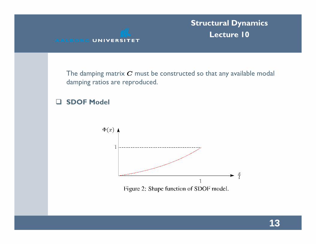
The damping matrix must be constructed so that any available modal damping ratios are reproduced.
� SDOF Model
1313

Structural Dynamics
Lecture 10
The displacement field is approximated as:
The shape function is taken as:
1414
Since, the generalized coordinate may be interpreted as the tip displacement of the blade.

Structural Dynamics
Lecture 10
The derivatives of the shape function become:
1515
The kinematic boundary conditions and the mechanical boundary condition (vanishing bending moment at the tip) are fulfilled. The mechanical boundary condition (vanishing shear force) is not fulfilled. The chosen shape function is considered acceptable.
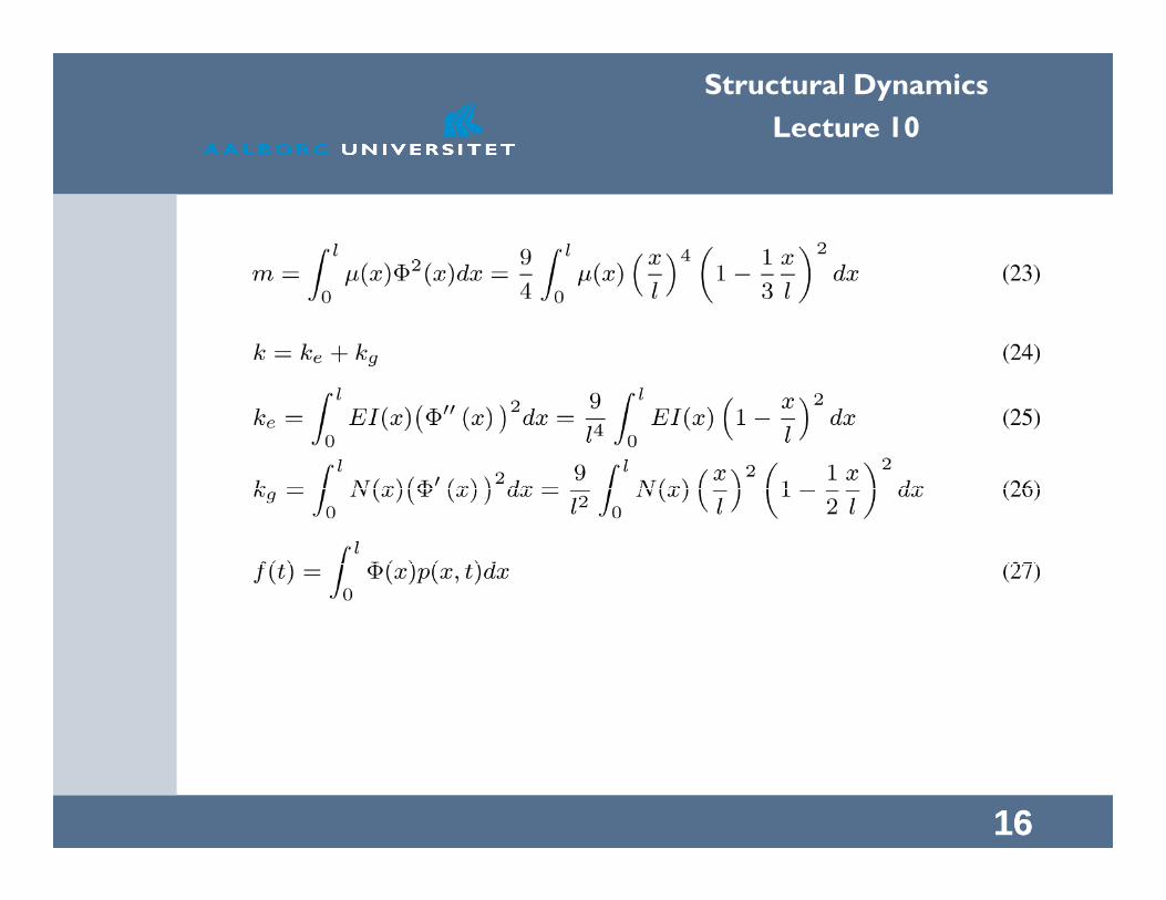
The mass, the stiffness and the dynamic load of the SDOF model becomes, cf. Eqs. (11), (13-15) and (16):
Structural Dynamics
Lecture 10
1616

Structural Dynamics
Lecture 10
� Example 1 : Rotating cantilever beam with constant cross-section
1717
The axial force becomes, cf. (3)

Structural Dynamics
Lecture 10
The mass and stiffnesses become, cf. (23-26):
1818
The angular eigenfrequency at becomes:

Structural Dynamics
Lecture 10
The exact values become, cf. Lecture 9, Eq. (69):
The numerical estimate (30) is an upper-bound due to Rayleigh’s principle.
1919
The angular eigenfrequency at becomes:
The increase in the angular eigenfrequency depends on the fraction . The factor is rather accurate, because the numerical
estimates of and are both upper-bounds, so the fraction is somewhat balanced.

Structural Dynamics
Lecture 10
� 2DOF Model
2020
The displacement field is approximated as:

Structural Dynamics
Lecture 10
The shape functions are taken as:
It follows from Fig. 4 that the coordinates and may be
2121
It follows from Fig. 4 that the coordinates and may be
interpreted as the displacement and the rotation of the tip.
The derivatives of the shape functions become:

Structural Dynamics
Lecture 10
The kinematic boundary conditions and are fulfilled. None of the shape functions fulfill the
2222
are fulfilled. None of the shape functions fulfill the mechanical boundary conditions and
.
The mass- and the stiffness matrices and the load vector of the 2DOF model become, cf. Eqs. (11), (13-15) and (16):

Structural Dynamics
Lecture 10
2323

Structural Dynamics
Lecture 10
2424

Structural Dynamics
Lecture 10
� Example 2: 2DOF model of a rotating cantilever beam
The cantilever beam shown in Fig. 3 is considered again using a 2DOF model with the shape function given by (34).
The mass- and stiffness matrices becomes, cf. Eqs. (28), (37), (38) and (39):
2525

Structural Dynamics
Lecture 10
The angular eigenfrequencies follows from the frequency condition, cf. Lecture 4, Eq. (43):
If the centrifugal stiffening effect is ignored ( ), the following angular eigenfrequencies are obtained:
2626
eigenfrequencies are obtained:
Both are upper-bounds to the exact results as given by (31) as a result of the Rayleigh principle. The 1st angular eigenfrequencies is acceptable, but the 2nd is somewhat too big.

Structural Dynamics
Lecture 10
� Introduction to the Finite Element Method
The finite element method is far the most general and applied numerical method for solving structural dynamic problems. The method is based on the division of the structure into a finite number of elements, each of which are required to be in dynamic equilibrium.
The so-called displacement (compatible) formulation of the method can be
2727
The so-called displacement (compatible) formulation of the method can be considered as a generalization of the displacement interpolation method described above.
Local dynamic equilibrium equations will only be derived for plane Bernoulli-Euler beam finite elements based on analytical dynamics. The geometric stiffness of the axial force will be ignored.

Structural Dynamics
Lecture 10
� Equations of Motion of a Plane Bernoulli-Euler Beam Element
2828

Structural Dynamics
Lecture 10
� : Nodal displacements and rotations. Degrees of freedom of the element.
� : Reaction forces and moments. These must balance the external loads, the inertial loads and the internal elastic and damping loads.
� : Bending stiffness around the -axis and mass per unit length. Both are constant along the beam element.
2929
� : Length of beam element.
� : Displacement field in the -direction.
� : Dynamic load per unit length in the -direction.
The basic idea is to interpolate the displacement field, so this is compatible with the nodal displacements , in the -direction, and the nodal rotations , in the -direction:

Structural Dynamics
Lecture 10
Cubic (Hermite) polynomial interpolation:
3030

Structural Dynamics
Lecture 10
where the shape functions are given as:
3131
The shape function have been illustrated in Fig. 6.

Structural Dynamics
Lecture 10
(47) may be presented on the matrix form::
3232
� : Element degrees-of-freedom vector.
Structural Dynamics
Lecture 10
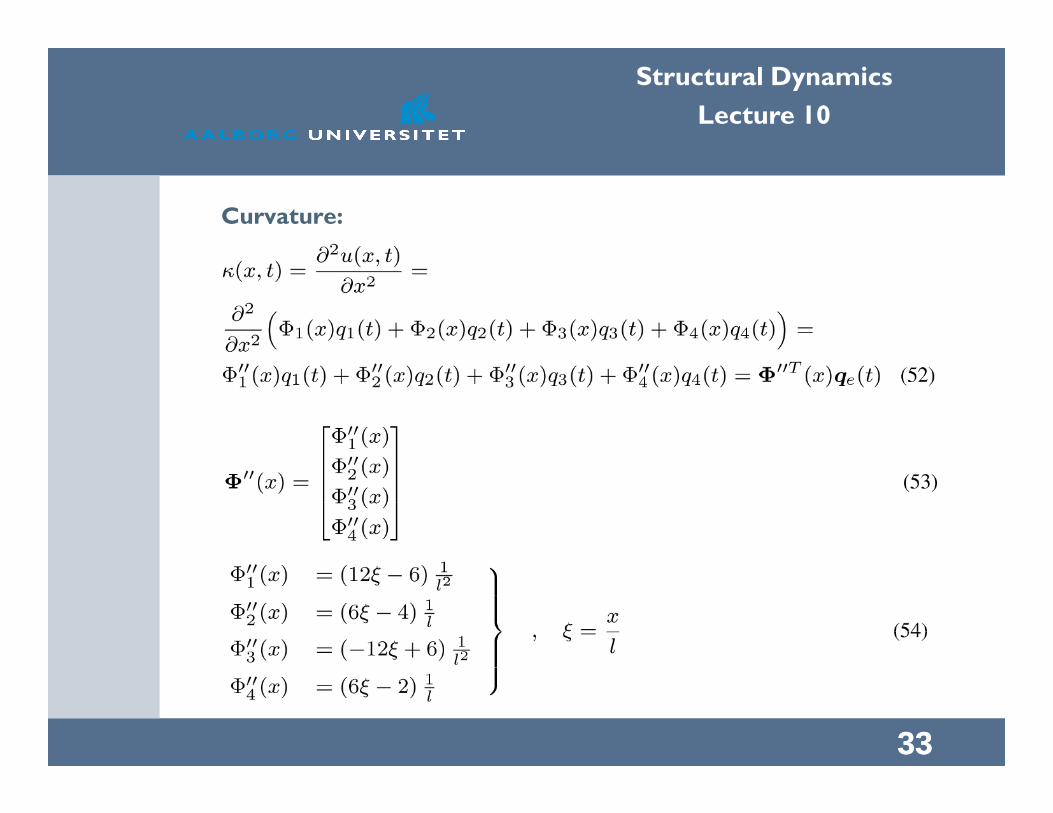
Curvature:
3333

Structural Dynamics
Lecture 10
Kinetic and potential energy of a deformed beam element:
The kinetic energy expressed in the degrees of freedom of the beam element becomes:
3434
Structural Dynamics
Lecture 10
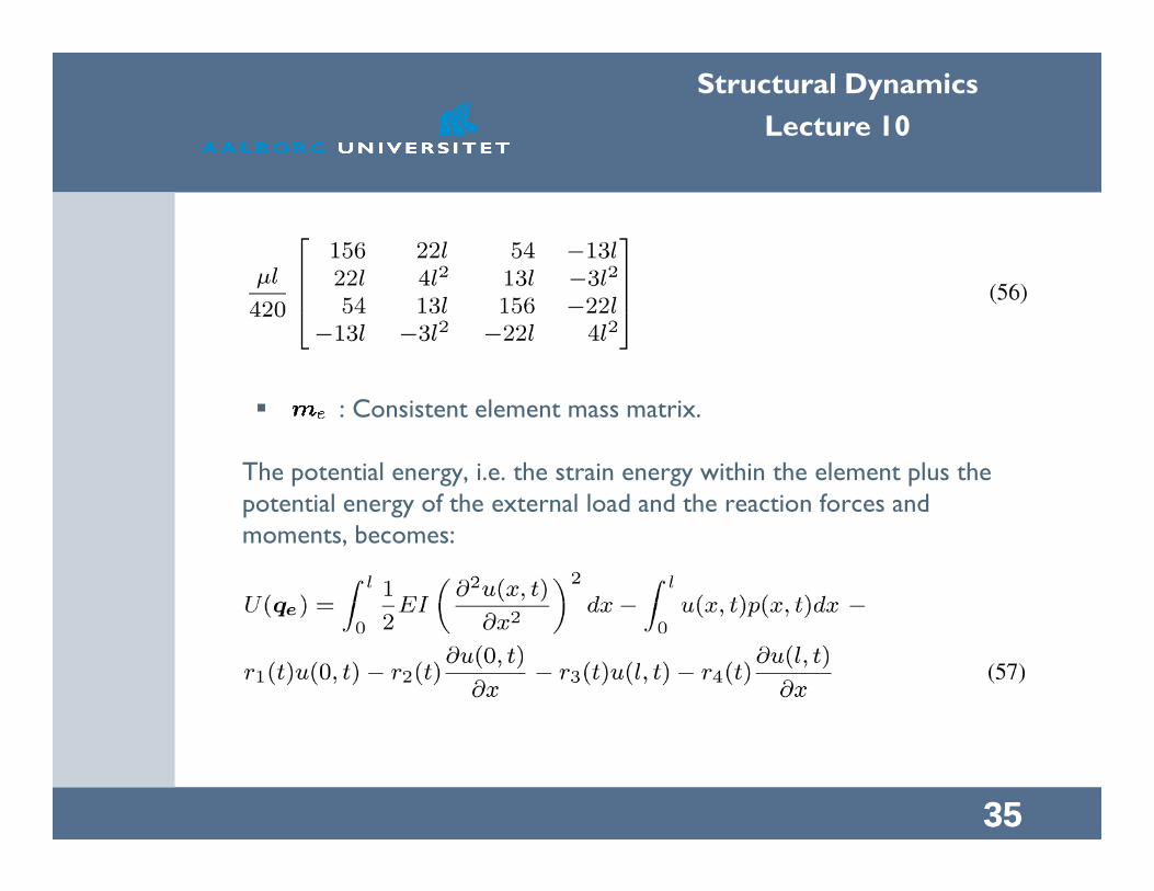
� : Consistent element mass matrix.
3535
The potential energy, i.e. the strain energy within the element plus the potential energy of the external load and the reaction forces and moments, becomes:

Structural Dynamics
Lecture 10
Insertion of (46), (49) and (52) provides:
3636

Structural Dynamics
Lecture 10
3737
� : Element stiffness matrix.
� : Element load vector.
� : Element reaction vector.
The load vector (60) is only valid for a constant dynamic load per unit length, .

Structural Dynamics
Lecture 10
Lagrange’s equations of motion:
Lecture 4, Eqs. (10), (13):
3838
� : Element damping matrix. (Rayleigh damping).

Structural Dynamics
Lecture 10
� Example 3: Calculation of element load vector
3939
The element load vector is calculated for the triangular load per unit length as shown in Fig. 7.

Structural Dynamics
Lecture 10
It can be shown that the reaction forces and moment as given by Eq. (63) for are in static equilibrium with the specified triangular load,
4040
for are in static equilibrium with the specified triangular load, corresponding to .

Structural Dynamics
Lecture 10
� Global Equations of Motion
4141
� : Local coordinate system attached to the beam element.
� : Global coordinate system.
� : Local components of degrees-of-freedom vector.
Dimension: .
� : Global components of degrees-of-freedom vector.
Dimension: .

Structural Dynamics
Lecture 10
and are related as:
Then, the inverse relation of (40)?? becomes
4242
Then, the inverse relation of (40)?? becomes
� : Angle from global -axis to local -axis in the positive -
direction (counter clock-wise).

Structural Dynamics
Lecture 10
The matrix is orthonormal (the column vectors have the length and are mutually orthogonal). Then:
Then, the inverse relation of (64) becomes:
4343
Then, the inverse relation of (64) becomes:
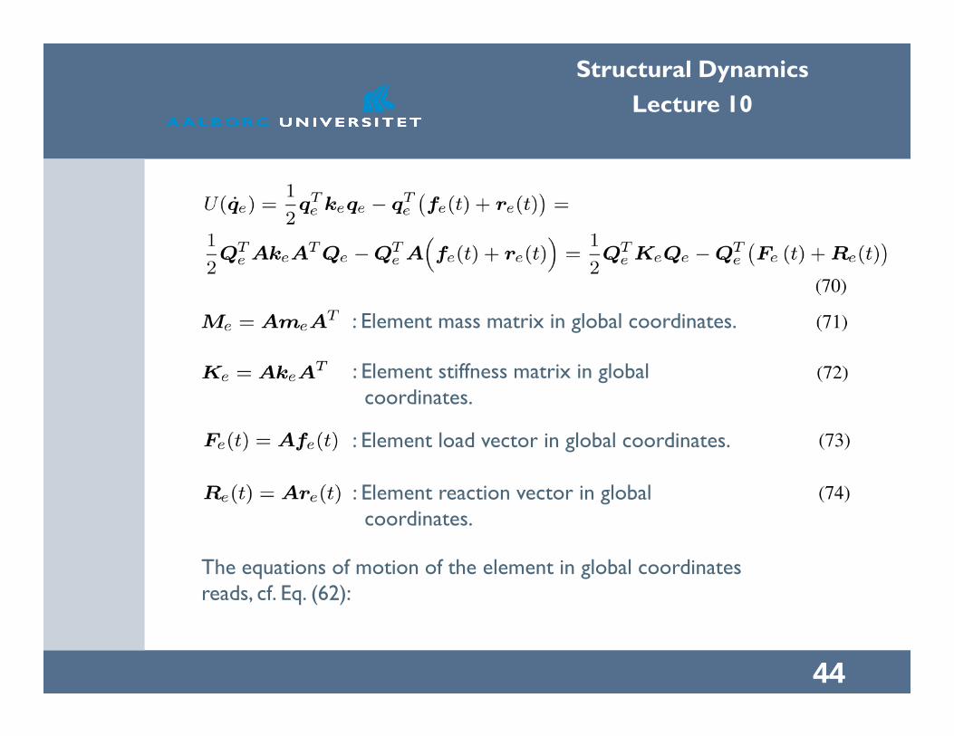
The kinetic energy and potential energy of the element as given by (55) and (58) may be expressed in global components, using (68):
Structural Dynamics
Lecture 10
: Element stiffness matrix in global
: Element mass matrix in global coordinates.
4444
: Element stiffness matrix in global coordinates.
: Element load vector in global coordinates.
: Element reaction vector in global coordinates.
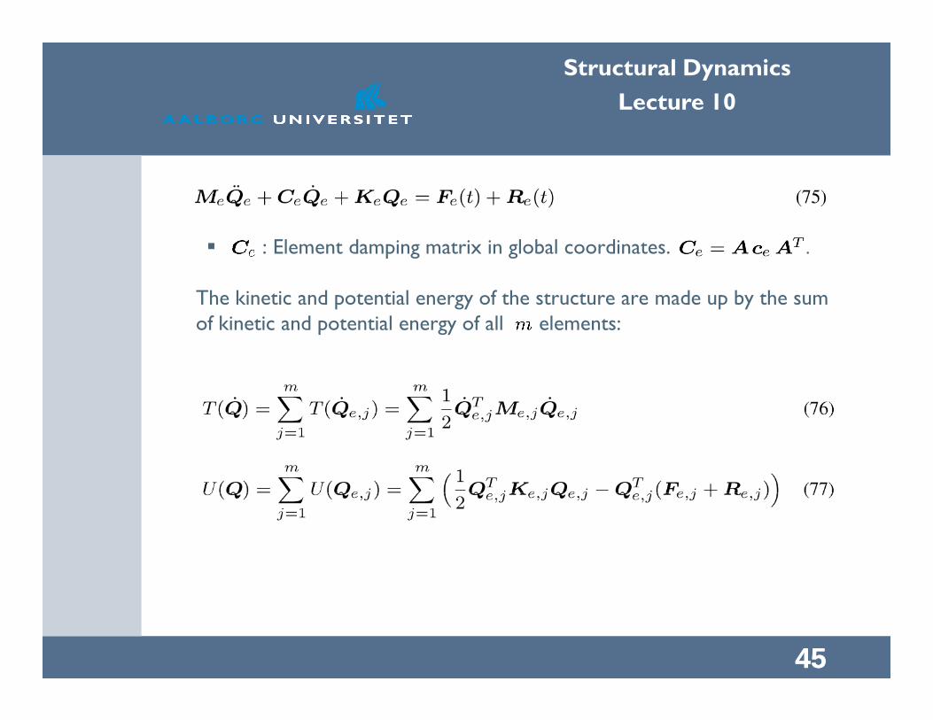
The equations of motion of the element in global coordinatesreads, cf. Eq. (62):
Structural Dynamics
Lecture 10
� : Element damping matrix in global coordinates. .
The kinetic and potential energy of the structure are made up by the sum of kinetic and potential energy of all elements:
4545

Structural Dynamics
Lecture 10
Displacement and rotation components of adjacent elements at the interface are identical. The non-trivial degrees of freedom from the nodes of the structure may be assembled in the vector:
4646
� : Number of nodes in the structure.
The dimension of becomes , where denotes the number of degrees of freedom per node. stores the degrees of freedom related to node . For a plane beam element this amounts to two displacement and one rotational degree of freedom. Since the structure is fixed at node , we have .

Structural Dynamics
Lecture 10
At the interface between elements the components of the reaction forcesin the summation in (77) vanishes mutually. Only at the support
nodes a net contributions occur, which are stored in vector .
Then, (76) and (77) may be written as:
4747
� : Global mass matrix. Dimension: .
� : Global stiffness matrix. Dimension: .
� : Global load vector. Dimension: .
� : Global reaction vector. Dimension: .

Structural Dynamics
Lecture 10
Most components of are zero. Non-vanishing components only occur at the support nodes, and represent the reaction forces and reaction moments. The global equations of motion of the structure become:
4848

Structural Dynamics
Lecture 10
Structure of and :
4949

Structural Dynamics
Lecture 10
Structure of and for a cantilever beam supported at node :
5050

Structural Dynamics
Lecture 10
The subvector of dimension determines the reaction forces and moment at the fixation. These are determined by the first ndofequations of (81) in combination with . The remaining equations determine the internal degrees of freedom.
5151

Structural Dynamics
Lecture 10
� Example 4: Cantilever beam modelled with two beam elements
5252
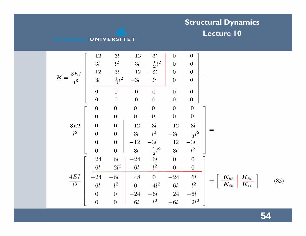
Fig. 9 shows a plane Bernoulli-Euler cantilever beam with constant mass per unit length and constant bending stiffness around the -axis. The undamped eigenfrequencies are calculated by modelling the
beam with two elements of the length .
From (56), (59), (82), (83) follows:

Structural Dynamics
Lecture 10
5353
Structural Dynamics
Lecture 10
5454
Structural Dynamics
Lecture 10
5555
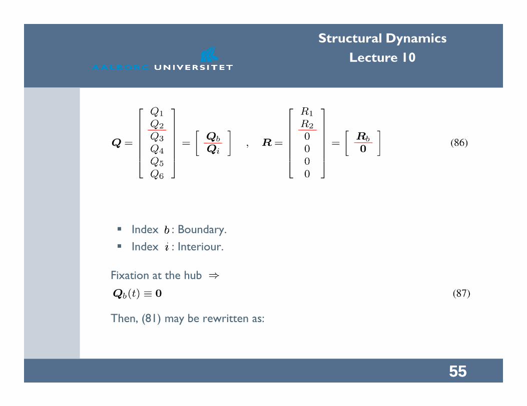
� Index : Boundary.
� Index : Interiour.
Fixation at the hub
Then, (81) may be rewritten as:

Structural Dynamics
Lecture 10
The undamped angular frequencies follow from the characteristic equation, see Lecture 4, Eq. (43):
5656
The solutions of (89) become:

Structural Dynamics
Lecture 10
The corresponding exact solutions become, see (31) and Lecture 9, Eq. (69):
5757
Only the lowest two eigenfrequencies are accurately calculated. In any case the numerical determined eigenfrequencies are upper bounds to the exact solutions, because compatible finite elements have been used (a consequence of the Rayleigh principle).
(MATLAB_2_Ex2)

Structural Dynamics
Lecture 10
Summary of Lecture 10
� Dynamical Modelling of Structures
� Shape functions must fulfil the kinematic boundary conditions . The mass matrix, stiffness matrix and the load vector are
obtained by equating the kinetic energy and potential energy of the continuous and the discrete systems.
� SDOF model. A single shape function.
5858
� SDOF model. A single shape function.
� 2DOF model. Two shape functions.
Top Related