


Languages
Pages
Legal

Stellar Feedback and Chemical Evolution in Dwarf Galaxies
Andrew J. Emerick
Submitted in partial fulfillment of the
requirements for the degree
of Doctor of Philosophy
in the Graduate School of Arts and Sciences
COLUMBIA UNIVERSITY
2019

c©2019
Andrew J. EmerickAll rights reserved

ABSTRACT
Stellar Feedback and Chemical Evolution in Dwarf
Galaxies
Andrew J. Emerick
Motivated by the desire to investigate two of the largest outstanding problems in galactic
evolution – stellar feedback and galactic chemical evolution – we develop the first set of
galaxy-scale simulations that simultaneously follow star formation with individual stars and
their associated multi-channel stellar feedback and multi-element metal yields. We devel-
oped these simulations to probe the way in which stellar feedback, including stellar winds,
stellar radiation, and supernovae, couples to the interstellar medium (ISM), regulates star
formation, and drives outflows in dwarf galaxies. We follow the evolution of the individual
metal yields associated with these stars in order to trace how metals mix within the ISM
and are ejected into the circumgalactic and intergalactic media (CGM, IGM) through out-
flows. This study is directed with the ultimate goal of leveraging the ever increasing quality
of stellar abundance measurements within our own Milky Way galaxy and in nearby dwarf
galaxies to understand galactic evolution.
Our simulations follow the evolution of an idealized, isolated, low mass dwarf galaxy
(Mvir ∼ 109 M�) for ∼ 500 Myr using the adaptive mesh refinement hydrodynamics code
Enzo. We implemented a new star formation routine which deposits stars individually
from 1 M� to 100 M�. Using tabulated stellar properties, we follow the stellar feedback
from each star. For massive stars (M∗ > 8 M�) we follow their stellar winds, ionizing
radiation (using an adaptive ray-tracing radiative transfer method), the FUV radiation which

leads to photoelectric heating of dust grains, Lyman-Werner radiation, which leads to H2
dissociation, and core collapse supernovae. In addition, we follow the asymptotic giant
branch (AGB) winds of low-mass stars (M∗ < 8 M�) and Type Ia supernovae. We investigate
how this detailed model for stellar feedback drives the evolution of low mass galaxies. We find
agreement with previous studies that these low mass dwarf galaxies exhibit bursty, irregular
star formation histories with significant feedback-driven winds.
Using these simulations, we investigate the role that stellar radiation feedback plays in
the evolution of low mass dwarf galaxies. In this regime, we find that the local effects of
stellar radiation (within ∼ 10 pc of the massive, ionizing source star) act to regulate star
formation by rapidly destroying cold, dense gas around newly formed stars. For the first
time, we find that the long-range radiation effects far from the birth sites are vital for carving
channels of diffuse gas in the ISM which dramatically increase the effect of supernovae. We
find this effect is necessary to drive strong winds with significant mass loading factors and
has a significant impact on the metal content of the ISM.
Focusing on the evolution of individual metals within this galaxy, it remains an out-
standing question as to what degree (if any) metal mixing processes in a multi-phase ISM
influence observed stellar abundance patterns. To address this issue, we characterize the
time evolution of the metal mass fraction distributions of each of the tracked elements in
our simulation in each phase of the ISM. For the first time, we demonstrate that there are
significant differences in how individual metals are sequestered in each gas phase (from cold,
neutral gas up to hot, ionized gas) that depend upon the energetics of the enrichment sources
that dominate the production of a given metal species. We find that AGB wind elements
have much broader distributions (i.e. are poorly mixed) as compared to elements released in
supernovae. In addition, we demonstrate that elements dominated by AGB wind production
are retained at a much higher fraction than elements released in core collapse supernovae

(by a factor of ∼ 5).
We expand upon these findings with a more careful study of how varying the energy and
spatial location of a given enrichment event changes how its metal yields mix within the
ISM. We play particular attention to events that could be associated with different channels
of r-process enrichment (for example, neutron star - neutron star mergers vs. hypernovae) as
a way to characterize how mixing / ejection differences may manifest themselves in observed
abundance patterns in low mass dwarf galaxies. We find that – on average – the injection
energy of a given enrichment source and the galaxy’s global SFR at the time of injection
play the strongest roles in regulating the mixing and ejection behavior of metals. Lower
energy events are retained at a greater fraction and are more inhomogeneously distributed
than metals from more energetic sources. However, the behavior of any single source varies
dramatically, particularly for the low energy enrichment events. We further characterize
the effect of radial position and local ISM density on the evolution of metals from single
enrichment events.
Finally, we summarize how this improved physical model of galactic chemical evolution
that demonstrates that metal mixing and ejection from galaxies is not uniform across metal
species can be used to improve significantly upon current state of the art galactic chemical
evolution models. These improvements stand to help improve our understanding of galactic
chemical evolution and reconcile outstanding disagreements between current models and
observations.
Contents
List of Figures v
Acknowledgments xvii
1 Introduction 1
1.1 Ingredients of Galactic Chemical Evolution . . . . . . . . . . . . . . . . . . . 5
1.1.1 Hydrodynamics . . . . . . . . . . . . . . . . . . . . . . . . . . . . . . 7
1.1.2 Nucleosynthesis . . . . . . . . . . . . . . . . . . . . . . . . . . . . . . 8
1.1.3 Radiative Processes and Chemistry . . . . . . . . . . . . . . . . . . . 12
1.1.4 Star Formation . . . . . . . . . . . . . . . . . . . . . . . . . . . . . . 13
1.1.5 Stars in Simulations . . . . . . . . . . . . . . . . . . . . . . . . . . . 14
1.1.6 Stellar Feedback . . . . . . . . . . . . . . . . . . . . . . . . . . . . . . 15
1.2 Observations of Local Group Dwarf Galaxies . . . . . . . . . . . . . . . . . . 20
1.2.1 Known Dwarf Galaxies of the Local Group . . . . . . . . . . . . . . . 21
1.2.2 Metals in Local Group Dwarfs . . . . . . . . . . . . . . . . . . . . . . 22
1.2.3 Leo P: A Case Study . . . . . . . . . . . . . . . . . . . . . . . . . . . 24
1.3 Onezone Models of Galactic Chemical Evolution . . . . . . . . . . . . . . . . 25
1.4 Structure of Dissertation . . . . . . . . . . . . . . . . . . . . . . . . . . . . 27
i

2 Simulating an Isolated Dwarf Galaxy with Multi-Channel Feedback and
Chemical Yields from Individual Stars 30
2.1 Introduction . . . . . . . . . . . . . . . . . . . . . . . . . . . . . . . . . . . . 30
2.2 Methods . . . . . . . . . . . . . . . . . . . . . . . . . . . . . . . . . . . . . . 34
2.2.1 Hydrodynamics and Gravity . . . . . . . . . . . . . . . . . . . . . . . 35
2.2.2 Chemistry and Cooling Physics . . . . . . . . . . . . . . . . . . . . . 36
2.2.3 Star Formation Algorithm . . . . . . . . . . . . . . . . . . . . . . . . 38
2.2.4 Stellar Properties . . . . . . . . . . . . . . . . . . . . . . . . . . . . . 40
2.2.5 Stellar Feedback and Chemical Yields . . . . . . . . . . . . . . . . . . 40
2.3 Galaxy Initial Conditions . . . . . . . . . . . . . . . . . . . . . . . . . . . . . 51
2.4 Results . . . . . . . . . . . . . . . . . . . . . . . . . . . . . . . . . . . . . . . 53
2.4.1 Morphological Structure and Evolution . . . . . . . . . . . . . . . . . 53
2.4.2 Star Formation Rate and Mass Evolution . . . . . . . . . . . . . . . . 56
2.4.3 ISM Properties . . . . . . . . . . . . . . . . . . . . . . . . . . . . . . 60
2.4.4 Interstellar Radiation Field . . . . . . . . . . . . . . . . . . . . . . . 63
2.4.5 Outflow Properties . . . . . . . . . . . . . . . . . . . . . . . . . . . . 67
2.4.6 Metal Evolution . . . . . . . . . . . . . . . . . . . . . . . . . . . . . . 71
2.5 Discussion . . . . . . . . . . . . . . . . . . . . . . . . . . . . . . . . . . . . . 75
2.5.1 Comparison to Observed Low Mass Dwarf Galaxies . . . . . . . . . . 75
2.5.2 Missing Physics . . . . . . . . . . . . . . . . . . . . . . . . . . . . . . 81
2.5.3 Detailed Stellar Evolution and Binary Stars . . . . . . . . . . . . . . 83
2.6 Conclusion . . . . . . . . . . . . . . . . . . . . . . . . . . . . . . . . . . . . . 84
2.A Gas Phases of the ISM . . . . . . . . . . . . . . . . . . . . . . . . . . . . . . 87
2.B Stellar Radiation Properties . . . . . . . . . . . . . . . . . . . . . . . . . . . 87
2.C Typical Gas Densities in Supernova Injection Regions . . . . . . . . . . . . . 88
ii

2.D Cooling and Heating Rates . . . . . . . . . . . . . . . . . . . . . . . . . . . . 91
2.E H− Photodetachment . . . . . . . . . . . . . . . . . . . . . . . . . . . . . . . 94
2.F Resolution Study . . . . . . . . . . . . . . . . . . . . . . . . . . . . . . . . . 97
3 Stellar Radiation is Critical for Regulating Star Formation and Driving
Outflows in Low Mass Dwarf Galaxies 102
3.1 Introduction . . . . . . . . . . . . . . . . . . . . . . . . . . . . . . . . . . . . 102
3.2 Methods and Initial Conditions . . . . . . . . . . . . . . . . . . . . . . . . . 105
3.3 Results . . . . . . . . . . . . . . . . . . . . . . . . . . . . . . . . . . . . . . . 107
3.4 Discussion . . . . . . . . . . . . . . . . . . . . . . . . . . . . . . . . . . . . . 111
3.5 Conclusion . . . . . . . . . . . . . . . . . . . . . . . . . . . . . . . . . . . . . 115
4 Metal Mixing and Ejection in Dwarf Galaxies is Dependent on Nucleosyn-
thetic Source 117
4.1 Introduction . . . . . . . . . . . . . . . . . . . . . . . . . . . . . . . . . . . . 117
4.2 Methods . . . . . . . . . . . . . . . . . . . . . . . . . . . . . . . . . . . . . . 122
4.3 Results . . . . . . . . . . . . . . . . . . . . . . . . . . . . . . . . . . . . . . . 125
4.3.1 Preferential Ejection of Metals from the ISM . . . . . . . . . . . . . . 127
4.3.2 Mixing and Distribution of Metals in the ISM . . . . . . . . . . . . . 131
4.4 Discussion . . . . . . . . . . . . . . . . . . . . . . . . . . . . . . . . . . . . . 139
4.4.1 Physical Interpretation of the PDF . . . . . . . . . . . . . . . . . . . 139
4.4.2 Comparison with Previous Studies of Metal Mixing . . . . . . . . . . 142
4.4.3 Timescale Dependence of AGB Ejecta . . . . . . . . . . . . . . . . . 143
4.4.4 Impact on Stellar Abundance Patterns . . . . . . . . . . . . . . . . . 146
4.4.5 Do These Results Apply to More Massive Galaxies? . . . . . . . . . . 147
4.4.6 Implications for Exotic Enrichment Sources . . . . . . . . . . . . . . 149
iii

4.4.7 Individual Stars vs. Averaged Yields . . . . . . . . . . . . . . . . . . 150
4.5 Conclusions . . . . . . . . . . . . . . . . . . . . . . . . . . . . . . . . . . . . 151
4.A Density PDF . . . . . . . . . . . . . . . . . . . . . . . . . . . . . . . . . . . 153
4.B Resolution Comparison . . . . . . . . . . . . . . . . . . . . . . . . . . . . . . 155
5 Mixing Properties of Individual Enrichment Sources 157
5.1 Introduction . . . . . . . . . . . . . . . . . . . . . . . . . . . . . . . . . . . . 157
5.2 Methods . . . . . . . . . . . . . . . . . . . . . . . . . . . . . . . . . . . . . . 159
5.2.1 Mixing Experiment Setup . . . . . . . . . . . . . . . . . . . . . . . . 160
5.3 Results . . . . . . . . . . . . . . . . . . . . . . . . . . . . . . . . . . . . . . . 161
5.3.1 Enrichment of the ISM and CGM . . . . . . . . . . . . . . . . . . . . 162
5.3.2 Homogeneity of Mixing . . . . . . . . . . . . . . . . . . . . . . . . . . 166
5.3.3 Event-by-Event Variation . . . . . . . . . . . . . . . . . . . . . . . . 170
5.3.4 Dependence on Radial Position . . . . . . . . . . . . . . . . . . . . . 172
5.3.5 Variation with Local ISM Conditions . . . . . . . . . . . . . . . . . . 174
5.3.6 Variation with SFR . . . . . . . . . . . . . . . . . . . . . . . . . . . . 176
5.4 Discussion and Conclusions . . . . . . . . . . . . . . . . . . . . . . . . . . . 177
6 Conclusion 181
6.1 A New Model for Galactic Chemical Enrichment . . . . . . . . . . . . . . . . 182
6.2 Stellar Radiation Feedback in Dwarf Galaxies . . . . . . . . . . . . . . . . . 183
6.3 Mixing and Ejection of Individual Metals . . . . . . . . . . . . . . . . . . . . 184
6.4 Mixing Behavior of Single-Sources . . . . . . . . . . . . . . . . . . . . . . . . 186
6.5 Future Work . . . . . . . . . . . . . . . . . . . . . . . . . . . . . . . . . . . . 187
Bibliography 190
iv

List of Figures
1.1 The periodic table of elements colored by the relative fraction of the astro-
physical source for each element. Image Credit: Figure 1 of Johnson (2019). 9
1.2 The Leo P dwarf galaxy. Left: Hi contours from the Very Large Array (VLA)
at 32” resolution overlaid on top of an optical Large Binocular Telescope
image. 32” is the lowest resolution Hi observation available of Leo P from
the VLA, which best traces diffuse, warm (T ∼ 103 K) Hi in the galaxy and
exhibits the full spatial extent of its gas content. This image is adopted from
the top-left panel of Figure 4 in Bernstein-Cooper et al. (2014). Right: Hα
emission (contours) overlaid on top of a Hubble Space Telescope (HST) optical
image. The Hii region analyzed in McQuinn et al. (2015b) to obtain gas-phase
metallicities is the blue clump of Hα towards the bottom of the image. This
image is adopted from Figure 10 of Evans et al. (2019). Note the inversion in
the vertical axes between the left and right panels. . . . . . . . . . . . . . . . 24
v
2.1 Edge-on views of our dwarf galaxy at four different times in its evolution, 0,
150, 300, and 500 Myr after the beginning of star formation. Shown are the
density weighted projection of number density (top row), temperature slices
(second row), HI column density (third row), and H2 column density (fourth
row). Each individual main sequence star particle is shown in the number
density projections as a single white dot. . . . . . . . . . . . . . . . . . . . . 55
2.2 Same as Fig. 2.1, but showing face-on views. . . . . . . . . . . . . . . . . . . 57
2.3 The total gas scale height at various times throughout the simulation. These
times match the images in Figs. 2.1 and 2.2. . . . . . . . . . . . . . . . . . . 58
2.4 Left: The SFR and core collapse SN rate in our dwarf galaxy in 10 Myr bins.
Broken portions of this histogram are time periods with no star formation or
supernovae. Note that the SN rate has been scaled by a factor of 100 to fit
on the same vertical axis as the SFR. Right: The evolution of the total gas
mass (black), HI mass (blue), H2 mass (orange), and stellar mass (red) in the
disk of our galaxy over time. . . . . . . . . . . . . . . . . . . . . . . . . . . . 59
2.5 The temperature vs. number density phase diagram of our dwarf galaxy simu-
lation showing all gas interior to 0.25 Rvir, averaged over a 50 Myr period from
t = 300 Myr to t = 350 Myr. The dashed lines are lines of constant pressure,
separated by factors of 10. The region in the lower right corner indicates our
density and temperature thresholds for star formation. . . . . . . . . . . . . 62
2.6 The evolution of the mass and volume fractions for each phase of the model
galaxy’s ISM. See Appendix 2.A for definitions of each phase. . . . . . . . . 63
vi

2.7 Azimuthally averaged radial profiles of the ISRF in the mid-plane of our galaxy
in two different bands, time-averaged over 50 Myr from 300 – 350 Myr. Here
we define the midplane as within 2.5 dx of z = 0, or 4.5 pc. The top panel
gives Go, the flux of radiation between 6–13.6 eV normalized to the value in
the solar neighborhood, shaded between minimum and maximum values at
each position, with the average shown as a black line. The bottom panel gives
the HI ionizing stellar radiation flux. Since this radiation is tracked directly
through radiative transfer, the minimum value at all radii is 0 at some point.
For this reason we only shade between the first quartile and maximum values.
HeI ionizing radiation is very similar to HI ionizing radiation, with a small
vertical offset, and is not shown for clarity. In the top panel, the minimum of
the vertical axis is the UVB value of Go. . . . . . . . . . . . . . . . . . . . . 65
2.8 Single-snapshot 2D radial profile plots at 300 Myr of the ISRF in two flux
bands, Go and HI ionizing radiation, illustrating the full dynamic range of
radiation flux at a given radius in the galaxy. Here, we include all gas within
the mid-plane of our dwarf galaxy. Since a majority of the mass of the galaxy
is in the cold phase (see Fig. 2.5), and is therefore optically thick to HI ionizing
radiation, it does not show up in the HI ionizing radiation diagram. This gas
readily appears in the Go diagram since we assume it to be optically thin,
though we do apply a localized shielding approximation. . . . . . . . . . . . 66
2.9 Spherical mass outflow rates (Eq. [2.7]) and mass loading rates over time at
4 different radii from the galaxy. . . . . . . . . . . . . . . . . . . . . . . . . . 68
vii

2.10 The time averaged radial velocity distribution of outflowing material external
to the disk and within the virial radius of our dwarf galaxy. This is averaged
over the same time interval as Fig. 2.7. The outflowing material is multiphase,
broken into WNM, WIM, and HIM. See Section 2.4.3 for definitions of these
regimes. We note that WNM is often labeled simply as “cold”, or gas below
T = 104 K. There is little to no outflowing mass in the CNM. . . . . . . . . 70
2.11 Left: Metal mass loading factor (see Eq.[ 2.8]) at the same radii as in Fig. 2.9.
This is the ratio between the metal outflow rate and the metal production rate.
Right: The fraction of metals contained in the disk, CGM, and outside the
halo of our dwarf galaxy over time. In both panels, we consider the total mass
of all individually tracked metal species, which is zero at initialization, not
the aggregate total metallicity field, which is non-zero at initialization. . . . 72
2.12 Three slices in the mid-plane of our dwarf galaxy at 300 Myr after the start
of star formation showing the variation in gas phase metal abundances. The
left slice gives the ratio of the abundance between N and O, normalized to the
solar abundance, while the number density and temperature are shown on the
right. In each, we mark massive stars with active stellar winds as white points
and SNe and AGB-phase enrichment events that occurred in the preceding 5
Myr as black stars and orange diamonds respectively. . . . . . . . . . . . . . 74
viii

2.13 The Kennicutt-Schmidt law (top) and extended Schmidt law (bottom) rela-
tionships for our galaxy as measured every megayear, plotted as points colored
by time, with dark / purple early and light / green late. See text for details
of the calculation. Recent observations from the SHIELD sample (Teich et al.
2016) are plotted as black points with error bars. On the left, we also give
the best fit line to galaxies from the FIGGS sample from Roychowdhury et al.
(2014), and on the right we also show the best fit line and 1 σ errors from Shi
et al. (2011). There is no clear correlation with time in this diagram. . . . . 77
2.B.1Radiation properties for our model stars, showing the ionizing photon lumi-
nosities for HI (top left) and HeI (top right) for each star, the FUV (middle
left) and Lyman-Werner (middle right) luminosities, and finally the average
ionizing photon energy for HI (bottom left) and HeI (bottom right). Note,
we only track radiation from stars above 8.0 M�, which dominate over less
massive stars, even when accounting for IMF weighting. . . . . . . . . . . . . 89
2.C.1Left: Distribution of peak (orange) and average (black) gas densities in the
injection region of each of the SNe from the simulation. Right: Distribution
of the radius of the pressure-driven snowplow phase for each SN assuming a
uniform medium at either the peak or average density in the injection region.
The vertical lines show one and 4.5 cell widths. This shows that a fraction of
these SNe are certainly unresolved, with RPDS less than a single cell size, and
somewhat more don’t satisfy the 4.5 cell criterion, but the majority are well
resolved. . . . . . . . . . . . . . . . . . . . . . . . . . . . . . . . . . . . . . . 91
ix

2.D.1The absolute value of the net cooling or heating rate in two models that
account for self-shielding of primordial gas against a metagalactic UV back-
ground. Our model (black) uses self-consistent metal line cooling rates, and
is compared to an incorrect model (orange) that adopts the uncorrected (i.e.
optically thin) metal line cooling rates. The regimes where heating dominates
are plotted with dashed lines for clarity. . . . . . . . . . . . . . . . . . . . . 92
2.D.2The total heating (dotted) and cooling (dashed) rates extracted from the
core of a Jeans-length sized cloud irradiated by a Haardt & Madau (2012)
metagalactic UV background as modeled in Cloudy. The absolute value of
the net cooling or heating rate is shown with solid lines. . . . . . . . . . . . . 94
2.E.1The final H2 mass fraction in a grid of one-zone Grackle cooling models run
with the same Grackle parameters and metallicity as our full hydrodynamics
simulation. Each model is held at a uniform density n = 10 cm−3. Each model
varies either the H− photodetachment rate or the Lyman-Werner background
over their respective UVB values by a given scale factor. Contours give factors
of ten change in the H2 fraction. We note the regime below 1.0 on each axis is
somewhat unphysical, and is never reached in our hydrodynamics simulations. 96
2.F.1A comparison of the SFR (left), disk gas mass (middle), and metal retention
(right) evolution for our fiducial run (solid), 3.6 pc run (dotted), 3.6 pc run
with a doubled initial supernova driving rate (dashed), and 7.2 pc run (dash-
dotted). The line colors in the left panel are for better clarity between the
SFRs. . . . . . . . . . . . . . . . . . . . . . . . . . . . . . . . . . . . . . . . 98
2.F.2Temperature-density phase diagrams for our 3.6 pc run (left) and 7.2 pc run
(right), as presented for our fiducial run in Fig. 2.5. . . . . . . . . . . . . . . 100
x

3.3.1 The star formation rate (left) and gas and stellar mass (right) of each of our
three simulations over time. Time bins with no star formation are left empty. 107
3.3.2 The total gas mass at n > 200 cm−3, our star formation density threshold. . 108
3.3.3 Top Left: The fraction of metals contained within the ISM of each galaxy
(blue) and the fraction ejected beyond the virial radius (orange). As in Fig-
ure 3.3.1, the fiducial run is given as solid lines, while the noRT and shortrad
are dash-dotted and dashed respectively. Top Right: The mass outflow
rate for each run at 0.25 Rvir (solid) and Rvir (dashed). Bottom: The mass
loading factor η calculated as the outflow rate divided by the SFR averaged
over 100 Myr. Inclusion of diffuse ionization makes an order of magnitude
difference in η in this case. . . . . . . . . . . . . . . . . . . . . . . . . . . . 110
3.4.1 Edge-on slices of each simulation showing gas number density (left), tem-
perature (middle), and hydrogen ionization fraction (right) 17 Myr after the
formation of the first star in each run. Each panel is 4 kpc x 4 kpc. See
Emerick et al. (2018a) for a movie of this evolution. . . . . . . . . . . . . . . 112
3.4.2 Same as Figure 3.4.1, but at 40 Myr. . . . . . . . . . . . . . . . . . . . . . . 113
4.3.1 Top: The mass fraction of each metal species in the full simulation box con-
tained in the halo, gas in the galaxy disk, and stars. Bottom: The mass
fraction of species within the disk alone in each phase of the ISM (bottom).
The leftmost bar in each plot shows the sum of all metals. . . . . . . . . . . 126
xi
4.3.2 The fraction of total mass in each metal species produced by each of the
four possible nucleosynthetic channels in our model. These channels differ
in both when metals are ejected, as determined by stellar evolution, and the
phase of the ISM into which they are ejected. We note that the minimal
contribution from Type Ia SNe for the iron-peak elements is because no older
stellar population was initialized, so only 16 of them have exploded by the
end of our 500 Myr simulation. . . . . . . . . . . . . . . . . . . . . . . . . . 128
4.3.3 The volume-averaged gas number densities within 20 pc of a given event (top)
and vertical position above/below the disk (bottom) within 1 Myr before the
event. . . . . . . . . . . . . . . . . . . . . . . . . . . . . . . . . . . . . . . . 130
4.3.4 The numerical PDFs (solid histograms) and the associated log-normal +
power-law fits (dashed lines) for a subset of the elements tracked in our sim-
ulation in each of the four gas phases defined in Section 4.3.1: CNM (dark
blue), WNM (light blue), WIM (light orange), HIM (red), and all the gas in
the ISM (black). For clarity, each distribution is normalized to the mode of
the full-disk PDF (black) and is centered on the median value of the full-disk
PDF. We note the vertical axis normalization is such that integrating over the
shown PDF gives the mass fraction of that phase in the disk. Since the CNM
dominates the mass fraction of our galaxy, the black curve is often obscured
at low metal fractions. . . . . . . . . . . . . . . . . . . . . . . . . . . . . . . 135
4.3.5 Time evolution of three different statistics for the full distributions of O (top)
and Ba (bottom) in each phase of our simulation. The panels show log10 of
the median (left), the difference, in dex, between the mean and the median
(middle), and the 90th decile and 10th decile difference in dex (right). . . . . 137
xii

4.4.1 The fraction of a given metal ejected through AGB winds at various times for
a model of a single-age stellar population at Z = 10−4 metal mass fraction,
without continuing star formation. We only show a sample of some of the
elements dominated most by AGB enrichment at late times. The horizontal
line marks a 50% contribution. . . . . . . . . . . . . . . . . . . . . . . . . . . 145
4.4.2 The separation (in dex) of each star’s oxygen fraction from the median value
of the CNM oxygen mass fraction PDF for the time within 1 Myr (our time
resolution) of each star’s formation time. The median deviation is given in the
plot for stars formed after the initial star formation and enrichment period
(120 Myr.) . . . . . . . . . . . . . . . . . . . . . . . . . . . . . . . . . . . . . 148
4.A.1The mass-weighted (left) and volume weighted (right) density PDFs of our
dwarf galaxy at an arbitrarily chosen time of 250 Myr. The total distribution
is given in black, sub-divided by the contributions of the individual phases in
the ISM. . . . . . . . . . . . . . . . . . . . . . . . . . . . . . . . . . . . . . . 154
4.B.1Resolution comparison of two lower resolution runs giving the log difference
between the 90th decile and 10th decile in dex for the metal PDFS of O and
Ba across all phases. Compare to Figure 4.3.5. . . . . . . . . . . . . . . . . . 156
5.3.1 Time evolution of the fraction of metals in each phase of the ISM (colored lines;
CNM: dark blue, WNM: light blue, WIM: orange, HIM: red), the galaxy’s disk
(black, dashed), and the CGM (black, solid) as averaged across all events at
a given Eej. The fractions are all normalized to the total amount of metals
initially injected in each event. The individual ISM phases sum to the black,
dashed line. . . . . . . . . . . . . . . . . . . . . . . . . . . . . . . . . . . . . 163
xiii

5.3.2 Time evolution of the fraction of enrichment source metals contained in the
CGM over time (left), and the fraction of metals in the CNM relative to just
those metals retained in the ISM for each enrichment source (right). These
are the same as the lines in Figure 5.3.1, but the CNM lines are normalized
by the black, dashed total ISM line in Figure 5.3.1. . . . . . . . . . . . . . . 166
5.3.3 Time evolution of the difference (in dex) between the mean metal mass fraction
of each source and the median metal mass fraction of each source in all of the
gas in the ISM (left) and in the CNM only (right). . . . . . . . . . . . . . . . 168
5.3.4 A summary of the results presented in Figure 5.3.2 and Figure 5.3.3 that
demonstrates the significant variation in fCGM, fCNM/fDisk, and the mean-
median separate at fixed injection energy. The points give the average values
at each energy at two different times, while the error bars show the min/max
values at each energy. The points at different times have been offset slightly
along the horizontal axes for clarity. Since they are only two points, we show
the results from I E52 r0 and I E52 r300 without averaging. . . . . . . . . . 171
5.3.5 The dependence of fCGM and fCNM/fDisk on the radial position of each event
at two different times in the evolution of the galaxy. The meaning of each
point, the error bars, and colors are the same as in Figure 5.3.4. . . . . . . . 173
5.3.6 The variation of fCGM, fCNM/fDisk, and the spread of the metal fraction PDFs
in the ISM as a function of the local ISM number density (n) within the
injection region of the event just prior (within 0.1 Myr) of the event. Points,
lines, and line colors mean the same as shown in Figure 5.3.4 . . . . . . . . . 175
xiv
5.3.7 The same as Figure 5.3.2, but comparing across both sets of runs with dif-
ferent SFRs. Comparing across line colors for a fixed linestyle compares the
difference the global SFR has on the average enrichment evolution for both
fCGM and fCNM/fDisk. . . . . . . . . . . . . . . . . . . . . . . . . . . . . . . . 178
xv

(This page left intentionally blank.)
xvi
ACKNOWLEDGMENTS
To my wife Ellen, who moved across the country for me to NYC (and across the country
again in the next few months), who has patiently put up with all of my travel and time away
at conferences in the past few years, who has worked longer hours at much more demanding
jobs than the work I have put into this Dissertation, and who has continued to support me
through this entire journey, all just so that I could pursue my dream. A simple “thank you”
is entirely insufficient to repay her for these sacrifices, but it is a good thing I have the rest
of my life to show how grateful I am.
To my family who have continued to support me in countless ways. In many ways my
parents are directly responsible for me pursuing a career in Astronomy. They enabled me to
have a good education throughout my life that prepared me well for graduate school. But
maybe more importantly, they provided me with my first exposure to the wonders of the
Universe which gave me the desire to pursue the path that led me to where I am today.
I have had many research advisors over the years, but am most indebted to my thesis
advisors, Greg and Mordecai, and my committee, Mary and Kathryn. Their thoughts,
advice, and encouragement over the past six years have been invaluable. This Dissertation is
as much a testament of my formation as a scientist as it is of the quality of their mentorship.
I would also like to thank my various undergraduate thesis advisors at the University of
Minnesota, Larry Rudnick, Tom Jones, and Priscilla Cushman, my REU advisor at Texas
A&M University, Ralf Rapp, and Pablo Yepes at Rice University.
I want to thank all of the other graduate students at Columbia that I have overlapped with
over the years. This includes especially Sarah, Steven, and Dan, and also Susan, Andrea,
Munier, Alejandro, Jeff, and Adrian. Their support and advice – and shared laughs and
beers – already make me look back on this time with fond memories.
xvii

While I have spent much of my time working in my office(s) at either Columbia, AMNH,
or the Flatiron Institute, a surprising fraction of this Dissertation and the published works
it is based upon were written outside of these places. I want to thank and acknowledge the
many coffee shops, bars, breweries, and the work space in my climbing gym in which I have
been surprisingly productive in times when I found my office uninspiring.
Thank you to everyone I have met in the NYC climbing community who have collectively
helped keep me sane throughout my time in graduate school. Over the past few years I have
learned the importance of a proper work-life balance, and climbing has helped me keep
that balance (... maybe a bit too well...). Thank you especially to my regular climbing
partners – Daniel Negless, Hunter Whaley, Dennis Kramer, and Lauren Anderson – who
I’ve trusted with my life countless times, and the handful of other astronomer-climbers that
I’ve climbed with throughout graduate school (Jeff Andrews, Matt Wilde, Lauren Anderson,
Dan D’Orazio, Dan Foreman-Mackey, and Andrea Derdzinski).
I would like to thank the numerous developers and contributors to the open-source soft-
ware packages without which this Dissertation would not be possible. This includes more
general software, such as Python, IPython, NumPy, SciPy, Matplotlib, HDF5,
h5py, and deepdish, and more astronomy-specific projects, yt, Enzo, Grackle, As-
troPy, and Cloudy. In particular I would like to thank the many developers of yt,
Enzo, and Grackle who have helped answer questions, debug code, review my pull re-
quests, and implement new features on my behalf throughout this process. This includes:
Britton Smith, Nathan Goldbaum, John Wise, Matt Turk, Greg Bryan, Simon Glover, Mu-
nier Salem, Cameron Hummels, Christine Simpson, Brian O’Shea, and others who I may
have forgotten.
Finally, I would like to thank you – the reader – for deciding that this Dissertation is
worth your attention.
xviii

2019, New York, NY
xix

Chapter 1
Introduction
The most exciting phrase to hear in science, the one that heralds discoveries, is not“Eureka!” but “Now that’s” funny
– Isaac Asimov
Debugging is twice as hard as writing the code in the first place. Therefore, ifyou write the code as cleverly as possible, you are, by definition, not smart enoughto debug it
– Brian W. Kernighan
Galaxies are amalgamations of gas and stars embedded in dark matter halos. They are
formed over cosmic time as the products of the hierarchical assembly that follows from the
collapse of the primordial density fluctuations which arose after the Big Bang. The gravita-
tional pull of dark matter – as predicted from ΛCDM cosmology – controls the hierarchical
growth of structure in the Universe. While, broadly speaking, the evolution of baryons is
dominated by this pull, the beautiful simplicity of ΛCDM cosmology is muddied by their
existence. The complexities of hydrodynamics, magnetohydrodynamics, thermodynamics,
chemistry, radiative processes, and nucleosynthesis – or, “astrophysics” for short – drives
1
these deviations and gives rise to the Universe that we observe. In spite of a concerted effort
spanning nearly a century, we are far from a self-consistent theory of galaxy evolution (see
Somerville & Dave (2015) and Naab & Ostriker (2017) for recent reviews). It is understand-
ing the rich set of physics that formed our own Galaxy and the countless galaxies scattered
throughout the Universe that motivates this work.
A substantial slice of modern astrophysics has been devoted towards understanding the
chemical evolution – the abundances of individual elements in space and time – of the
Universe. With the exception of H, He, and trace amounts of light elements, all of the
elements in the Universe are produced in nuclear reactions associated with stellar evolution
– in the cores of stars – and released in stellar winds, asymptotic giant branch (AGB) winds
of low mass stars, SNe, and more exotic sources, like neutron star - neutron star mergers (NS-
NS). See Nomoto et al. (2013), Thielemann et al. (2017), and Frebel (2018) for recent reviews
on this topic as it applies to studies of galactic and stellar evolution. Much work has been
done in studying the global metallicity evolution of galaxies through the mass-metallicity
relationship (e.g. Lequeux et al. 1979; Tremonti et al. 2004; Lee et al. 2006; Zahid et al.
2012; Andrews & Martini 2013), the metallicity gradient in our own and nearby galaxies
(e.g. Searle 1971; Shaver et al. 1983; Belfiore et al. 2017; Sanchez-Menguiano et al. 2017),
and detailed stellar abundances in nearby dwarf galaxies with spectroscopically resolved
stars (see the review in Tolstoy et al. 2009). Yet in spite of increased number and quality
of observations tracing galactic chemical evolution, developing a complete model of galactic
chemical evolution is still a daunting task.
To give an impression of the difficulties involved, we outline a recipe for constructing a
complete model of galactic chemical evolution. One must first prescribe a galaxy’s connection
to its large scale structure to understand the inflow of pristine, metal-free gas and growth of
its gaseous disk, and the accretion (via mergers) of stars formed previously in galaxies hosted
2
by different dark matter halos. One can then worry about knowing where, when, how, and
with what masses stars form in the first place from this gas. This requires understanding the
hydrodynamic properties of the multi-scale, multi-phase turbulent interstellar medium (ISM)
and the radiative processes and chemistry that operate within the ISM. This in turn requires
one to toss in a detailed understanding of the stellar feedback physics – stellar radiation,
stellar winds, and SNe – that helps to regulate star formation by destroying cold, star forming
gas, driving the multi-phase structure of the ISM, and by driving outflows of gas into the
circumgalactic medium (CGM) around galaxies. Simultaneously, one must make the simple
step of nailing down a complete model of stellar structure, stellar evolution, the reaction
rates and cross sections of every nuclear reaction, and the lifetimes of individual isotopes.
Once all of this is understood, one can then color in the gas in the galaxy over time with the
individual metal yields of stellar populations released over their lifetime. With a complete
understanding of stellar feedback and the ISM, one can then be sure that they completely
capture the mixing of these metals in the ISM over time, and will produce a stellar population
with accurate metal abundance ratios. In addition, one would then produce realistic galactic
winds, removing the correct amount of metals from the galaxy and enriching the CGM and
the intergalactic medium (IGM). Finally, one can layer this model ad nauseum on top of
a ΛCDM model for the cosmological evolution of many galaxies, reproducing all observed
properties of galactic chemical evolution as a function of both mass and redshift..... Wait...
I forgot about magnetic fields, active galactic nuclei, and cosmic rays...
It should be obvious now to the reader why there remains so much to be learned about
galactic chemical evolution. Yet it is clear that this field offers an incredibly exciting test of
a wide range of physical processes.
The observational landscape today is primed for developing a more detailed understand-
ing of these processes. Recent observational campaigns such as SEGUE (Yanny et al. 2009),
3

RAVE (Kunder et al. 2017), the Gaia-ESO survey (Gilmore et al. 2012), APOGEE and
APOGEE2 (Majewski et al. 2010, 2016), GALAH (De Silva et al. 2015; Buder et al. 2018),
as well as upcoming observations, such as the Local Volume Mapper as part of SDSS-V,
have generated tremendous amounts of information on detailed stellar abundances and stel-
lar kinematics in our Milky Way and nearby Local Group dwarf galaxies. One of the most
powerful proposed uses of this enormous trove of data is chemical tagging (Freeman & Bland-
Hawthorn 2002), whereby stellar populations are analyzed in chemical space and 6D phase
space to identify co-eval and co-natal groups of stars. This process of galactic archeology
aims to break down and identify each distinct stellar component of our Galaxy, explaining
the process of their formation and evolution. Substantial work has been made recently to
determine the efficacy of this approach (e.g. Ting et al. 2012; Hogg et al. 2016; Jofre et al.
2017; Price-Jones & Bovy 2018; Armillotta et al. 2018), yet the physical processes that give
rise to stellar abundances as we observe them today are still uncertain.
Dwarf galaxies have been called the building blocks of the Universe, and represent some
of the best laboratories to study the fundamental physics of galactic evolution. From a
theoretical perspective, their small physical size, relatively quiet accretion history, and low
star formation rates make simulating their evolution in detail at high resolution substantially
less computationally intensive than more massive galaxies like the Milky Way. Although their
lower brightness limits the number of dwarf galaxies that we can observe, the abundance
and relative proximity of dwarf galaxies in the Local Group allows for a significant sample of
galaxies with resolved stellar populations. Observations of these resolved stellar populations
can be used to derive detailed star formation histories and chemical abundances that can
be used together to test our theoretical understanding of galactic chemical evolution in a
variety of contexts.
In order to better understand galactic chemical evolution as a whole, we study the detailed
4

process of metal enrichment in the ISM and the ejection of metals into the CGM through
high-resolution hydrodynamics simulations of individual galaxies. In the remainder of this
introduction, we discuss the physical process that we consider in constructing a complete
model of galactic evolution in Section 1.1 with an emphasis on how these processes are
treated in simulations, a summary of relevant observations of the nearby dwarf galaxies
relevant to this study in Section 1.2.1, a discussion of alternative approaches to modeling
galactic chemical evolution in Section 1.3, and an outline of the rest of this Dissertation in
Section 1.4.
1.1 Ingredients of Galactic Chemical Evolution
The following is a primer on how to model galactic evolution in hydrodynamics simulations.
We focus on the physics needed to simulate galaxies (cooling, heating, chemistry, star forma-
tion, feedback, etc.) as it pertains to the aspects of galactic chemical evolution examined in
this Dissertation. This is meant to be a broad overview of the physical processes treated in
such simulations, focusing more on aspects of their implementation rather than the deriva-
tion of theory behind each process. While important, the latter is beyond the scope of
this introduction and would readily turn into a full textbook. Focusing on implementation
gives a much more accurate representation of the actual work done and skills learned dur-
ing this Dissertation. This discussion includes a very brief overview of hydrodynamics and
the numerical methods used in this work in Section 1.1.1, nucleosynthesis and stellar evo-
lution in Section 1.1.2, radiative cooling and chemistry (actual chemistry) in Section 1.1.3,
star formation and star particles in Section 1.1.4 and Section 1.1.5, and stellar feedback in
Section 1.1.6.
But first, we note that Astronomy jargon is full of idiosyncrasies. As mentioned before,
5

the word “chemical” in “galactic chemical evolution” is a bit of a misnomer. This is com-
monly applied simply to refer to studies interested in the evolution of metal abundances
(either as a whole, or for individual isotopes) in galaxies over time, and less often to the
chemical reactions that those elements may participate in. Unfortunately “chemistry” is
often used with both meanings in the same work requiring context to decipher the intended
meaning. “Metals” refers broadly to every element except H and He. Throughout this Dis-
sertation we often refer to the metallicity (Z) of a galaxy, its gas, or its stars. This quantity
represents the total mass fraction of all metals – and is computed as such in our simulations
– but we note that it is generally impossible to measure the abundances of all metals in
astrophysical contexts outside our own Solar System (and even then, it is challenging). The
metallicity of our own Sun (Z�), for example, is still uncertain (Asplund et al. 2009). Instead,
most observational works adopt Fe as a proxy for total metallicity in stars (due to its many,
strong absorption lines), O as a proxy in gas-phase abundances in the ISM (as it is the most
abundant metal in the Universe and has convenient, strong emission lines), and O or C in
gas-phase abundances of the CGM when observed in absorption (primarily through the lines
OVI and CIV). These metallicity proxies are usually reported in some form of normalized
abundance ratio. For stellar metallicities, this is given in the form [A/B] = log(NA/NB)
- log(NA/NB)�, where N refers to the number of atoms of a given element (e.g. [Fe/H]).
Confusingly, gas-phase abundances are commonly reported as just log(NA/NB), often with
the somewhat arbitrary normalization of +12, or log(O/H) + 12, for example; converting
between the two definitions is straightforward (albeit annoying) and requires adopting a
value for the solar abundance. 1
1This is not to mention issues in normalization across methods of deriving these abundances... (e.g.Kewley & Ellison 2008).
6
1.1.1 Hydrodynamics
Astrophysical hydrodynamics simulations are first differentiated by the numerical methods
they employ to solve the Euler equations. These equations describe the time (t) evolution
of the energy density (E), density (ρ), pressure (p), and peculiar velocity (v) of a fluid:
δρ
δt+∇ · (ρv) = 0, (1.1)
δρv
δt+∇ · (ρvv + Ip) = 0, (1.2)
δE
δt+∇ · [(E + p)v] = 0. (1.3)
Historically, codes fall into one of two camps: 1) Eulerian grid-based codes, including
the popular codes / algorithms commonly in use (in some way) today such as Zeus (Stone
& Norman 1992), flash (Fryxell et al. 2000), ramses (Teyssier 2002), Athena (Stone
et al. 2008), art-II (Rudd et al. 2008), and Enzo (Bryan et al. 2014), and 2) particle-based
Lagrangian methods known as smooth particle hydrodynamics (SPH), such as Gadget
(Springel 2005), pkdgrav-2 (Stadel 2001), Gasoline (Wadsley et al. 2004), and Changa
(Menon et al. 2015). However, recent codes blur the lines between these distinctions with
new algorithms for solving the fluid equations on a moving-mesh (e.g. arepo Springel
2010), or meshless finite-mass / finite-volume methods (such as those implemented in Gizmo
Hopkins 2015). Traditionally these codes were designed to run exclusively on CPUs, but
significant work has been made recently to offload various portions onto GPUs, such as
gamer and gamer-2 (Schive et al. 2010, 2018), gpugas (Kulikov 2014), and cholla
(Schneider & Robertson 2015). Given the large variance in numerical methods, recent studies
have examined the differences between these numerical implementations (e.g. Agertz et al.
2007), including large-scale code comparison projects (e.g. Kim et al. 2014, 2016). While
7

developing even a notion of which code is “correct” is an ill-posed problem, these studies
have allowed for improvement across implementations and an insight into how numerical
methods themselves drive uncertainty in our understanding of astrophysical problems.
In this Dissertation, we make use of the adaptive-mesh refinement (AMR) hydrodynamics
code Enzo, as described in greater detail in Chapter 2. As it pertains to galactic chemical
evolution, however, the use of a grid-based code has the advantage that metals (which are
advected as passive scalars that follow the fluid-flow in the simulations) are allowed to mix
and diffuse naturally across fluid elements (grid cells). This is not possible in native SPH
implementations, yet is necessary to reproduce realistic galactic chemical evolution properties
as shown by multiple recent works testing implementations of diffusion in SPH simulations
(e.g. Shen et al. 2010; Revaz et al. 2016; Hirai & Saitoh 2017; Su et al. 2017; Escala et al.
2018). The disadvantage of the diffusion in Enzo, however, is that it is entirely numerical.
Therefore, its exact properties are challenging to characterize and are resolution dependent.
Throughout this Dissertation we attempt to account for the effects of resolution on our
results, but do not explicitly examine the properties of numerical diffusion itself.
1.1.2 Nucleosynthesis
A variety of nucleosynthetic processes occur within stars and during their deaths that lead
to the production of all of the elements in the periodic table. Different astrophysical sources
reach conditions that enable different nuclear reactions, as is well-illustrated in Figure 1.1.
This image shows the periodic table colored by the fractional importance of the astrophysical
source that produce each element. Due to the diversity in production sources across the
periodic table, multi-element metal abundance measurements in stars can be used to better
understand and constrain how and where each metal is produced. Exactly which reactions
occur where depend strongly on the initial abundances of elements in stars, their stellar
8
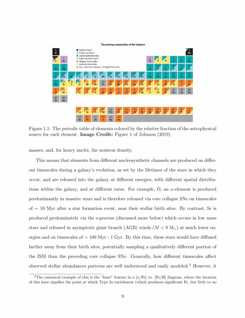
Figure 1.1: The periodic table of elements colored by the relative fraction of the astrophysicalsource for each element. Image Credit: Figure 1 of Johnson (2019).
masses, and, for heavy nuclei, the neutron density.
This means that elements from different nucleosynthetic channels are produced on differ-
ent timescales during a galaxy’s evolution, as set by the lifetimes of the stars in which they
occur, and are released into the galaxy at different energies, with different spatial distribu-
tions within the galaxy, and at different rates. For example, O, an α-element is produced
predominantly in massive stars and is therefore released via core collapse SNe on timescales
of ∼ 10 Myr after a star formation event, near their stellar birth sites. By contrast, Sr is
produced predominately via the s-process (discussed more below) which occurs in low mass
stars and released in asymptotic giant branch (AGB) winds (M < 8 M�) at much lower en-
ergies and on timescales of ∼ 100 Myr - 1 Gyr. By this time, these stars would have diffused
farther away from their birth sites, potentially sampling a qualitatively different portion of
the ISM than the preceding core collapse SNe. Generally, how different timescales affect
observed stellar abundances patterns are well understood and easily modeled.2 However, it
2The canonical example of this is the “knee” feature in a [α/Fe] vs. [Fe/H] diagram, where the locationof this knee signifies the point at which Type Ia enrichment (which produces significant Fe, but little to no
9

is not well understood how differences in where and with what energies these events occur
affect observed stellar abundance patterns. Investigating these differences is a key motivation
of this Dissertation.
As relevant to this work, we briefly summarize a few of the important nucleosynthetic
channels shown in Figure 1.1 and their sites. α-elements, notably O, Mg, Si, Ca, and Ti,
are produced during the lifetime of massive stars (O, Mg) or during the core collapse SN
explosion itself. In either case, these elements are synthesized through the capture of an α
nucleus, progressing towards increasingly heavier nuclei in intervals of 4/2 in mass/atomic
number (as α = 42He) from 8
4Be all the way to the stable 5226Fe and unstable 56
28Ni (which decays
to 5626Fe). The iron group elements, notably Fe, Mn, Co, and Ni, are produced predominately
in Type Ia SNe, with variations depending on a single vs. double degenerate scenario, the
initial composition of exploding white dwarf(s) (WD), and the dynamics of the explosion
itself.
The presence of these heavier elements in stars enables the formation of even heavier
nuclei through neutron capture. This is categorized into two processes, the slow (or s-)
and rapid (or r-) process. In the former, neutron densities are typically low enough that
the product of each neutron capture beta decays to a more stable isotope before capturing
another nucleon. In r-process, however, the rate of neutron capture exceeds beta decay,
allowing for the production of different, typically heavier, nuclei. The lighter heavy nuclei
elements (Rb through Pb, though with exceptions) are produced via the s-process and heavier
(Te through Bi, again, with exceptions) via the r-process, with notable overlap in certain
elements, such as Ba. The s-process occurs predominately in low mass (1-8 M�) stars and
is released at the end of their lives via AGB winds on time scales of 100’s of Myr up to 1
α elements) begins to have a significant contribution over core collapse SNe (rich in α elements, but notFe) (e.g. Matteucci & Brocato 1990; Geisler et al. 2005; Hill et al. 2018). The location of this knee in thisdiagram shifts for a given galaxy depending on its SFH.
10

Gyr. Exactly which elements are produced in a given AGB star varies with stellar mass
and depends strongly on metallicity, which determines the available heavy seed nuclei. Sr,
Y, Zr, and Ba, as well as C, N and F, are commonly used as observational tracers of this
nucleosynthetic channel.
The dominant origin of r-process enrichment is highly uncertain, though (as indicated
in Figure 1.1) possible channels include NS-NS mergers, neutron star - black hole mergers,
neutrino driven winds in core collapse SNe, and exotic SNe, such as magnetic, jet-driven SNe,
collapsars, hypernovae, and long-duration gamma-ray bursts (see Frebel 2018; Cowan et al.
2019, for recent reviews). Eu is the most commonly used (and easy to observe) unambiguous
observational tracer of r-process enrichment; Ba is also often studied as a tracer, but requires
care due to the significant contribution from s-process enrichment. More detailed spectra
(e.g. Ji & Frebel 2018) can trace many more of these elements, which can be used as an
important discriminator between nucleosynthetic models.
Finally, although the production of elements unaffected by the r-process are compara-
tively well understood, there are still large uncertainties in both nuclear reaction rates and
stellar evolution properties that affect the computed yields for any given element. As in-
cluding self-consistent nuclear reactions in the interior of stars is nearly computationally
impossible in galaxy-scale simulations, metal yields are generally included as averaged over
an entire stellar population (see Section1.1.5) as obtained from a tabulated set of yields. The
yields for a given star in a simulation are typically IMF-averaged, and occasionally mass and
metallicity dependent depending on the level of detail desired in the simulation. Often,
only the global metallicity is tracked in simulations, but tracking individual metal species
(especially C, O, and Si which can affect the chemistry and cooling physics in the ISM) is
becoming more common. The uncertainties across tabulated yields, however, mean there are
often significant variations and inconsistencies between tables produced by separate groups.
11

These can sometimes make interpreting the results of galactic chemical evolution models
challenging.
1.1.3 Radiative Processes and Chemistry
Radiative processes are of fundamental importance in properly modeling the diversity of
density, temperature, and ionization states in a multi-phase ISM. It is via radiative cooling
that gas, heated by gravitational accretion onto dark matter halos, can cool, condense,
become self-gravitating, and (eventually) collapse to form stars. Conversely heating, via
radiative absorption or scatterings, from stellar sources within galaxies and the extragalactic
sources that comprises the cosmic UV background (UVB, e.g. Haardt & Madau (2001, 2012);
Faucher-Giguere et al. (2011)). Tied to both of these processes is the actual chemistry that
occurs in the ISM, from the primordial chemical reactions between H, He, and free electrons
to substantially more complicated reactions that occur once significant amounts of metals are
present in the ISM (particularly, C, O, and Si). These metals by themselves act as additional
radiative coolants, which strongly dictate the shape of the cooling curve that helps establish a
multi-phase medium in the first place (e.g. McKee & Ostriker 1977). The molecules produced
in chemical reactions with these metals produce additional coolants in the ISM (Hollenbach
& McKee 1979), including dust, which has its own rich array of associated physical processes
(Omukai 2000; Omukai et al. 2005; Draine 2011).
A full, detailed model of radiative cooling, heating, non-equilibrium chemistry, and dust
is generally far too computationally expensive to include in galaxy-scale simulations. For this
reason, many large-scale cosmological simulations assume that all gas is optically thin and
that all molecules and ionization states exist in equilibrium. This allows for the quick use
of tabulated look-up tables for radiative cooling and heating, often produced using cloudy
(Ferland et al. 2013), that depend on gas density, temperature, metallicity, and redshift
12

(which sets the UVB heating rate). More complex simulations often track some number
(usually < 10) of species involved in primordial chemistry in order to better account for non-
equilibrium effects and H2 production, though with noted increases in memory requirements
and computational cost. Some of the most advanced models to-date can account for well
over 102 individual chemical reactions involving > 20 elements and molecules (e.g. Richings
& Schaye 2016; Richings & Faucher-Giguere 2018); but these are typically prohibitively
expensive to run on large scales. In this Dissertation we adopt the chemistry and radiative
cooling and heating physics models available in the newly developed, open-source library
GRACKLE (Smith et al. 2017). The exact physics included in our simulations are discussed
in greater detail in Chapter 2, but we note that improvements to GRACKLE have been
made as the direct result of the research conducted during this Dissertation.
1.1.4 Star Formation
In galaxy-scale hydrodynamics, the extreme computational cost of resolving the spatial scales
and gas densities required to directly follow star formation relegates this process to a sub-
grid model. Stars form from fluid elements that surpass a variety of threshold conditions at
an assumed rate and efficiency. Usually, simulators set these thresholds to fully encompass
gas whose Jeans-length (and thus dynamical behavior) becomes unresolved according to the
widely-used Truelove et al. (1997) criterion. Often, gas is required to surpass a simple mass
or number density threshold, on top of which simulators can also require that the local gas
cells be in a converging flow (∇ · v < 0), that gas surpass some virial threshold (describing
how bound a cloud may be) or that gas meet a minimum H2 mass fraction or that density
high enough to support H2 formation (e.g. Kuhlen et al. 2012). Once a fluid element is
flagged as star forming, simulators have a few options for how to compute the fraction and
rate at which gas is turned into stars. Briefly, some form of the following equation is usually
13

adopted to describe the star formation rate density,
ρSF = ερgas
t∗, (1.4)
where ρgas is the local gas density, ε is some fixed or variable star formation efficiency, and
the timescale, t∗, is often adopted as the local free fall time, or
t∗ = tff =
√3π
32Gρgas
. (1.5)
In many cases, ε is fixed to some small value (∼ 0.01) (Krumholz & Tan 2007) meant to
represent a galaxy-scale average of star formation efficiency, even though this may vary
significantly between individual molecular clouds (Grudic et al. 2018). High-resolution sim-
ulations, where the mass of stars that would form in a single time step (dt × SFR) is far
less than a single star particle mass, allow stars to form out of star forming fluid elements
stochastically (e.g. Goldbaum et al. 2015).
Recent work has demonstrated that variations in these implementations can lead to
dramatic differences in the outcome of the simulated galaxies (e.g. Hopkins 2013; Munshi
et al. 2018). However, it is generally found that the differences between implementations
decrease in simulations with sufficient resolution (∼ 10 pc or better spatial, or ∼ 100 M�
or better in mass) and with a sufficiently high density threshold for star formation (n >
100 cm−3) (Orr et al. 2018; Hopkins et al. 2017).
1.1.5 Stars in Simulations
Stars, particularly in large-scale cosmological simulations, are commonly represented as sim-
ple stellar populations (SSPs), or particles with IMF-averaged properties of stellar feedback
14

and metal enrichment. As demonstrated in Revaz et al. (2016), this approach is reasonable
so long as the mass of the star particle is large enough to fully sample the IMF (> 104 M�).
In high resolution simulations, particularly simulations of small, low-mass systems like dwarf
galaxies, this is no longer the case. This leads to inconsistencies in both the effective metal
yield of the modeled stars, and (often) an artificial reduction of the effects of stellar feedback.
Recent works have developed new models to address this issue, discretizing (rather than av-
eraging over) individual feedback events (e.g. Stinson et al. 2010; Hopkins et al. 2014, 2018;
Rosdahl et al. 2018) or accounting for stochastic sampling of the IMF (Hu et al. 2016, 2017;
Applebaum et al. 2018; Su et al. 2018). However, each of these methods utilizes a sub-grid
recipe in some fashion to improve upon the SSPs. On the other extreme are highly resolved
simulations which model star formation with “sink particles” (see for example Krumholz
et al. 2004; Federrath et al. 2010; Gong & Ostriker 2013; Bleuler & Teyssier 2014; Sormani
et al. 2017) that account for the gradual accretion of gas in the growth of a single star (or
group of stars) and protostellar feedback. These recipes are often computationally expen-
sive, however, restricting their use over long timescales (100’s to 1000’s of Myr or more) in
galaxy-scale simulations.
In this Dissertation, we develop the first implementation that breaks the SSP formalism
entirely by following stars as individual star particles sampled from an adopted IMF. This
allows us to place unprecedented detail on both the stellar feedback and metal yields associ-
ated with each star, spatially and temporally resolving differences in both of these channels
as a function of stellar mass and metallicity.
1.1.6 Stellar Feedback
The first models of galactic evolution produced galaxies with stellar masses far in excess
of what is observed in the Universe. From these initial works, it was clear that some form
15

of feedback process must take place to self-regulate star formation within galaxies. With
observations of metal abundances in the CGM around galaxies (see Tumlinson et al. 2017,
for a recent review), and of fast-moving outflows from star forming galaxies (see Veilleux
et al. 2005, for a review), it was additionally clear that some mechanism must exist to drive
these outflows. Stellar feedback became the clear physical mechanism to account for both of
these phenomena.3
Initial models for stellar feedback relied primarily on the energy injection from supernovae
(SNe, see Section 1.1.6.1) to regulate star formation and drive outflows, but it has become
clear that this mechanism alone cannot completely account for all of the star formation,
ISM, outflow, CGM, and even intergalactic medium (IGM) properties of observed galaxies
(see Somerville & Dave (2015) and Naab & Ostriker (2017) for recent reviews and more
detailed discussion of how feedback impacts outstanding problems in galactic evolution).
Other sources of effective stellar feedback have been identified (e.g. Agertz et al. 2013),
which serve to regulate star formation on different timescales and help develop an ISM and
CGM with different phase and ionization properties. This includes both stellar radiation
(Section 1.1.6.2) and stellar winds (Section 1.1.6.3).
Although not included in this Dissertation, for the sake of completeness, we mention a
few additional sources of stellar feedback that likely contribute to the full picture of galactic
evolution: 1) cosmic rays, 2) stellar binary evolution, and 3) hypernovae and other exotic
sources of feedback. First, a substantial amount of recent research has been dedicated to
the examination of SN-driven cosmic ray feedback (see Section 2.5.2.2 for a more detailed
discussion and references). In brief, cosmic rays can be a dominant source of heating in very
dense, optically-thick gas and act as a source of non-thermal pressure in the ISM, which
3Except maybe for more massive galaxies, where active galactic nuclei may play some role in regulatingstar formation and certainly play a role in driving outflows (e.g. Fabian 2012). We do not discuss this sourceof feedback further in this Dissertation aside from noting that it is another significant uncertainty in ourunderstanding of galactic evolution.
16

can drive galactic winds with qualitatively different phase structures (e.g. Salem et al. 2016).
Second, binarity is often ignored in models of stellar feedback. The effects of binary evolution
can dramatically extend the timescales over which ionizing radiation and SNe act in a newly
formed stellar population. Typically, this increases their total energy output and decreases
the ISM densities in which SN explode, increasing their effectiveness (see Section 2.5.3).
Third, exotic sources of stellar feedback, such as hypernovae, high-mass X-ray binaries, and
NS-NS mergers can also be a potentially important sources of feedback, particularly in the
lowest mass halos (e.g. Artale et al. 2015). However, the uncertainties in the frequency
and delay time distributions for when these events should occur, and their relative rarity,
preclude including these effects in this Dissertation.
1.1.6.1 SNFeedback
In the simplest model, SNfeedback is treated as the injection of pure thermal energy (and
mass) into the fluid element(s) that are host / closest to the chosen site of a SNexplosion.
In self-consistent models of star formation and feedback these sites are usually actual star
particles, but this does not have to be the case. The first models which included SNfeedback
lacked the spatial / mass resolution to resolve individual (or even collective) SN events. This
is the source of the commonly known “overcooling” problem, whereby too little energy is
injected into too much mass such that the affected region only reaches modest temperatures
(T . 105 K, as opposed to T > 107 K, or so). This temperature is right around the peak
of the cooling curve, and thus the energy is rapidly radiated away before it has time to
make a significant dynamical impact of the galaxy. This is still a problem today in large-box
simulations of cosmological volumes which have insufficient resolution to resolve individual
SNe. While some of the initial, ad-hoc fixes for this problem (e.g. turning off cooling for
some time in SN affected fluid elements or decoupling SN affected SPH particles from the
17

hydrodynamics for some time) are still in use today, some notable advancements have been
made to employ some combination of kinetic, momentum, and thermal energy feedback to
attempt to capture SNe in a more consistent fashion (e.g. Hopkins et al. 2014; Simpson et al.
2015; Hopkins et al. 2018).
High resolution simulations, like those developed in this Dissertation, can typically rely
on using pure thermal energy injection while still avoiding artificial overcooling.4 This is true
for simulations with typical spatial / mass resolutions better than a few pc / 10 M� (Simpson
et al. 2015; Hu 2018; Smith et al. 2018b). However, a spatial resolution requirement is a
density dependent statement; in this case SNe that occur in the densest gas (n > 102−3 cm−3)
may still be under-resolved and ineffective. In this case, accounting for feedback processes
from massive stars that occur before the first core collapse SN in a given star formation
event becomes critical (Hu et al. 2016). Including these physics, as discussed below, greatly
reduces the typical ISM densities in which SNe occur, greatly increasing the likelihood that
these events are well resolved.
1.1.6.2 Stellar Radiation
We only briefly discuss this method of feedback here, as it is discussed in much more detail
in both Chapters 2 and 3. In brief, Abbott (1982), Reynolds (1990), Leitherer et al. (1999),
Agertz et al. (2013), and others have demonstrated that stellar radiation accounts for a
substantial fraction of the total energy output of a stellar population. Ionizing photons
from young, massive stars can photoionize and heat the gas surrounding sites of recent star
formation. This pre-processes the local environment within which SNe occur, often increasing
the effectiveness of SNe in regulating star formation and driving outflows (Hu et al. 2016). In
addition, radiation pressure in the single-scattering limit (from UV photons) and rescattered
4This is advantageous because it is often substantially easier to implement than kinetic / momentuminjection methods while being less susceptible to numerical artifacts, especially for grid-based codes.
18

infrared photons has been used as an additional source of pre-SN feedback (e.g. Hopkins
et al. 2014). However, due in part to differences in how ionizing radiation is followed across
simulations, there is disagreement as to exactly how and in what conditions this acts as a
source of feedback (see Krumholz (2018) for a detailed examination of this problem).
Non-ionizing radiation also contributes to the regulation of star formation and the multi-
phase ISM. Far ultraviolet (FUV) photons contribute to gas heating via the photoelectric
heating of dust grains. This is a significant heating mechanism in higher metallicity envi-
ronments, like the Milky Way (Parravano et al. 2003; Wolfire et al. 2003), but may still
be important in setting the temperature floor of cold dense gas in lower mass galaxies
(Forbes et al. 2016; Hu et al. 2017). Lyman-Werner (LW) band radiation regulates the
H2 abundance, which is particularly important in low-metallicity environments where H2 is
a dominant coolant (e.g. Glover 2003; Wolcott-Green & Haiman 2012).5 As the goal of this
Dissertation is to develop an as-complete-as-possible model of galactic chemical evolution,
we account for each of these processes in some fashion.
The simplest way to model stellar radiation feedback is to apply an optically thin, ana-
lytic radiation profile, such as the galaxy-centered exponential photoelectric heating profile
used in Tasker & Tan (2009), or 1/r2 profiles from individual sources (e.g. Forbes et al.
2016). However, radiative transfer effects, such as gas self-shielding, are often important,
particularly for ionizing radiation. Solving the equations of radiative transfer directly in
simulations – as is done with ray tracing methods – is computationally expensive and scales
significantly with the number of sources. For this reason, approximate methods, such as
flux-limited diffusion, treat radiation as a fluid, removing the scaling of computational cost
with the number of sources. In this Dissertation, we follow the evolution of galaxies that
have at most 10 − 100 ionizing sources at one time, making it computationally feasible to
5And is arguably even more important when using star formation prescriptions that depend upon thelocal H2 mass fraction.
19
use the accurate adaptive ray-tracing radiative transfer method implemented in Enzo.
1.1.6.3 Stellar Winds
Stellar winds, in addition to stellar radiation, are a potentially important source of pre-SN
feedback that helps regulate star formation in / around the birth clouds of newly formed stars.
However, the hot (T > 106 K), fast (v ∼ 103 km s−1) winds from massive stars (Weaver et al.
1977) are challenging to model self-consistently in galaxy-scale simulations. For this reason,
there has been comparatively little research on how they affect global galaxy properties, even
though some models do include their energy injection in an integrated / approximate fashion
(e.g. Hopkins et al. 2014). However, stellar winds, from both massive stars and weaker winds
from the AGB phase of low mass stars, are important sources of metal enrichment. For this
reason we include stellar wind feedback in this Dissertation, albeit in a simplified fashion.6
1.2 Observations of Local Group Dwarf Galaxies
We are motivated by using a properly formed model for galactic chemical evolution in dwarf
galaxies to interpret and explain observations of Local Group dwarfs. As any good theoretical
work should maintain a close connection to the observations that motivate the study in the
first place in order to better make predictions for future observations, we devote some time
here to summarize relevant observations of Local Group dwarfs.
6Although we do not have conclusive results to this end, initial examination of our simulations has shownthat our stellar wind model is only globally important in simulations where radiation feedback is ignored. Itis thus likely sub-dominant to radiation feedback (Abbott 1982; McKee et al. 1984).
20

1.2.1 Known Dwarf Galaxies of the Local Group
The Milky Way and its local environment is host to a diverse collection of dwarf galaxies.
The properties of these galaxies have been nicely summarized in a recent review (Tolstoy
et al. 2009), and again in McConnachie (2012). However, the number of known Local
Group dwarf galaxies has increased dramatically since that time, particularly for the Milky
Way, whose known satellite population has more than doubled. This is due in large part
to tremendous improvements in our ability to detect galaxies on the faintest end of the
luminosity function, called ultrafaint dwarf galaxies (UFDs, Willman et al. 2005).7. The
Dark Energy Survey (e.g. Drlica-Wagner et al. 2015) and Hyper Suprime-Cam (e.g. Greco
et al. 2018) have made tremendous advances to this end, with the upcoming Large Synoptic
Survey Telescope expected to produce an even greater increase in the known population of
faint galaxies in the Local Group (Haynes 2019; Weisz & Boylan-Kolchin 2019).
While there is no true sharp transition below which a galaxy is considered “dwarf”,
historical definitions are based on luminosity cuts, using the SMC and LMC as rough anchor
points for the upper-end of the dwarf galaxy scale. Bullock & Boylan-Kolchin (2017) suggests
a delineation based on stellar mass. For this Dissertation, we follow this definition and
consider galaxies with M∗ < 109 M� as dwarf galaxies, and galaxies with M∗ < 105 M�
as UFDs. In general, dwarf galaxies are extremely dark matter dominated, with mass to
light ratios over 102 (Simon & Geha 2007; Strigari et al. 2008; Wolf et al. 2010), convert gas
into stars at a lower efficiency than more massive galaxies, and, for the lowest mass dwarf
galaxies, exhibit bursty star formation histories driven by stochasticity in the process of both
star formation and the effects of stellar feedback .
7See Simon (2019) for a recent review
21

1.2.2 Metals in Local Group Dwarfs
The first studies of stellar abundances in the Local Group focused on stars in nearby dwarf
spheroidals (dSph’s), and massive stars in the LMC, SMC, and similar, more massive dwarf
galaxies. These studies typically obtained abundances for only a small sample (∼ 10) stars,
limiting the extent to which they can be used to test models of galactic chemical evolution.
However, the advent of high-resolution spectrographs at both Keck and the Very Large
Telescope – capable of obtaining the spectra of many stars with a single pointing – have
dramatically increased the sample size of stellar abundances in nearby dwarf galaxies.
Stellar feedback drives outflows, galactic winds, from galaxies across all scales Dwarf
galaxies in particular, with their relatively shallow potential wells, are expected to drive
effective galactic winds (Mac Low & Ferrara 1999) with mass loading factors (η = Mout/SFR)
above 100 (Muratov et al. 2015; Christensen et al. 2018). Not only does this correspond to
a significant amount of mass outflow from these galaxies, but these winds should also carry
out a substantial amount of metals from these galaxies. In fact, the differences with which
different models for feedback-driven winds drive metals in outflows in low mass galaxies can
be an important constraint on the underlying physics (e.g. Wheeler et al. 2018; Agertz et al.
2019). Kirby et al. (2011b) used measurements of the stellar abundances in Local Group
dSph’s and their resolved star formation histories to determine that their stars contain less
than 5% of the metals synthesized in each galaxy. However, since these galaxies have lost their
gas through environmental processes as satellites of the Milky Way (primarily ram pressure
and tidal stripping), it was unclear if this loss could be attributed entirely to feedback.
However, using gas and stellar abundances McQuinn et al. (2015b) showed that Leo P – a
gas-rich Local Group dwarf galaxy – has also ejected ∼95% of its metals (see Section 1.2.3).
This is significant evidence for metal-enriched, feedback-driven galactic winds operating in
22

these low mass dwarf galaxies.
Finally, the low metallicities of the lowest mass dwarf galaxies make them ideal places to
better constrain large uncertainties in stellar nucleosynthesis (Frebel & Norris 2015; Frebel
2018). At these low metallicities, the number of possible enrichment events that could have
possibly contributed to the observed stellar abundances decreases significantly, increasing the
possibility of using these abundance patterns to constrain the yields of individual sources.
This is particularly true for exotic enrichment events, like those expected to be sources of
r-process elements, which are potentially so rare that only one or fewer events would be
expected in an individual low-mass galaxy.
The most prominent example of these types of studies has been of the UFD Reticulum
II, where Ji et al. (2016a) used the extreme r-process enhancement in its stars to argue in
favor of a NS-NS origin of r-process enrichment. This conclusion has been supported by
observations in additional Local Group dwarf galaxies (Duggan et al. 2018), but there is still
some disagreement as to the dominant source of r-process enrichment (e.g. Siegel et al. 2018).
Interestingly, the lack of these extreme r-process abundances in other UFDs suggests that
another source of r-process must exist (Ji et al. 2016c). Some of the significant uncertainties
in interpreting these observations lie with understanding how r-process elements mix within
the ISM and are ejected from low mass dwarf galaxies. Recent research has examined how
metals from individual enrichment events may mix and evolve in a variety of contexts (e.g.
Bland-Hawthorn et al. 2015; Ritter et al. 2015; Montes et al. 2016; Safarzadeh & Scannapieco
2017), but there is still much to be understood about this process. In particular, there
is still much to be gained from adapting insights from these types of simulations to the
modeling used to interpret observations of stellar abundances (as discussed in more detail in
Section 1.3).
23

Figure 1.2: The Leo P dwarf galaxy. Left: Hi contours from the Very Large Array (VLA)at 32” resolution overlaid on top of an optical Large Binocular Telescope image. 32” is thelowest resolution Hi observation available of Leo P from the VLA, which best traces diffuse,warm (T ∼ 103 K) Hi in the galaxy and exhibits the full spatial extent of its gas content.This image is adopted from the top-left panel of Figure 4 in Bernstein-Cooper et al. (2014).Right: Hα emission (contours) overlaid on top of a Hubble Space Telescope (HST) opticalimage. The Hii region analyzed in McQuinn et al. (2015b) to obtain gas-phase metallicitiesis the blue clump of Hα towards the bottom of the image. This image is adopted from Figure10 of Evans et al. (2019). Note the inversion in the vertical axes between the left and rightpanels.
1.2.3 Leo P: A Case Study
We dedicate this section to a specific Local Group dwarf galaxy, Leo P, as its observed
properties motivate the initial conditions of the simulations developed in this Dissertation.
This galaxy is remarkable for being one of the lowest mass dwarf galaxies with observed,
ongoing star formation. It is located at a distance of 1.62±0.15 Mpc (McQuinn et al. 2015a),
and was first characterized as part of the ALFALFA survey (Giovanelli et al. 2013; Rhode
et al. 2013; Skillman et al. 2013; McQuinn et al. 2013; Bernstein-Cooper et al. 2014). These
studies have characterized its star formation history as low and roughly continuous over the
24

age of the Universe (<SFR> = 4.3× 10⁻⁵ M� yr−1, McQuinn et al. 2015a), its stellar mass
(M∗ = 5.7 × 10⁵ M�, McQuinn et al. 2013), its Hi and dynamical mass (MHI(r < rHI) =
9.5 × 10⁵ M�, Mdyn(r < rHI) = 2.6 × 10⁷ M�, rHI ∼ 500 pc, Bernstein-Cooper et al. 2014),
and gas-phase abundances from an Hii region (12 + log(O/H) = 7.17±0.04 Skillman et al.
2013). HI, optical, and Hα observations of Leo P are shown in Figure 1.2.
We chose to focus on a Leo P like galaxy in our simulations in part to allow for compar-
isons to the work in McQuinn et al. (2015b), which makes an accounting of the total metals
(as traced by O) contained in the ISM and stars in Leo P, estimating the fraction that must
have been ejected over the lifetime of the galaxy. As of this writing, Leo P is one of the only
low mass dwarf galaxies with both gas-phase and stellar metal abundance measurements,
but there is ongoing work to greatly expand this sample in the near future.
1.3 Onezone Models of Galactic Chemical Evolution
This Dissertation utilizes high-resolution hydrodynamics simulations that are expensive to
run in terms of both wall-time (∼ weeks to months) and computational time (∼ 105−6
CPU hours). For this reason, it is computationally infeasible to directly explore many of the
uncertainties associated with each of the components of the model as discussed in Section 1.1.
For this reason, substantially cheaper semi-analytic models are valuable tools that can be
used to better understand galactic evolution.
One of the most common ways to model and understand the stellar populations of galax-
ies in high-dimensional chemical space is through simplified one-zone (or many-zone) mod-
els. This treatment extends back many decades (e.g. Schmidt 1963; Talbot & Arnett 1971;
Lynden-Bell 1975), where galaxies and their total metal abundances were treated in closed-
box systems of gas and stars. Over the intervening years these models have improved,
25

including prescriptions for gas outflow (a “leaky-box”) or gas inflow (an “accreting box”), or
both (a “bathtub” model, e.g. Finlator & Dave 2008; Bouche et al. 2010). The assumptions
that go into these models vary dramatically with complexity. Simple models can assume, for
example, that long-lived low mass stars do not contribute to metal enrichment while metals
from massive stars are instantaneously recycled into the galaxy’s gas reservoir (i.e. ignoring
stellar lifetimes) or that all metals mix instantly and homogeneously. More complex models
account for individual stellar lifetimes (to some degree), or may try and account for some
aspects of inhomogeneous mixing by constructing multi-zone models that may separate a
galaxy in radial bins (with or without mixing between bins), may account for a hot and cold
component separately (with mixing between the two), or account for separate ISM and CGM
components. The output of these models is typically the mean metal abundance evolution
within each of the tracked components. There is generally no self-consistent prescription to
account for the scatter in any abundance relationship in these models, which, when needed,
is often added ad-hoc in post-processing. Regardless of the assumptions that go into these
models, they are powerful tools that can be used to probe the general physical processes
that govern galactic chemical evolution, and explore the vast, uncertain parameter space
associated with the models that characterize these processes (e.g. Cote et al. 2017).
One final motivation of this Dissertation is to improve the assumptions within these
models by better characterizing the process of inhomogeneous mixing in the ISM, and the
coupling of metals to galactic winds and outflows. This is particularly important if the be-
havior differs between elements from different nucleosynthetic sites. In addition, this work
could be used to account for the spread and higher-order statistics of stellar abundance dis-
tributions, which would be a powerful tool for better leveraging the wealth of observations
in the Milky Way and Local Group. Yet, as discussed, the current state of the art prescrip-
tions for these processes are ad-hoc. Recent analytic work in Krumholz & Ting (2018) lays
26

down a framework to evaluate the correlation between individual metals in different galactic
environments and predicts that the correlations will differ for sources that trace different
nucleosynthetic sites (e.g. AGB wind vs. SNe). We characterize these differences in detail in
Chapter 4, laying the groundwork for how one could potentially incorporate this insight into
improving these models. We build upon this idea more in Chapter 5, and plan to explore
the connection between our simulations and analytic models in the future. Recent work by
Schonrich & Weinberg (2019) is a great example of how this could impact current models
for galactic chemical evolution. The authors show how adopting a two-phase model (hot
and cold ISM), along with parameters for how metals are injected and mix between the
phases whose values differ depending on nucleosynthetic origin of the metal, can reconcile
long-standing problems in understanding the r-process abundance evolution of stars in the
Milky Way. In fact, they argue that it would be impossible to reproduce observed r-process
abundances in the Milky Way (namely [Eu/Fe], [Eu/Si], and [Eu/Mg] as functions of [Fe/H])
with a standard one-phase model.
1.4 Structure of Dissertation
In this work we investigate the role of both stellar feedback and mixing in a multi-phase ISM
in driving galactic chemical evolution. Using a novel method for following star formation and
stellar feedback in galaxy-scale hydrodynamics simulations, we provide significant insight
into how individual metals from distinct nucleosynthetic sites enrich the ISM, how their
abundances are set and imprinted upon newly formed stars, and how they are ejected from
galaxies through galactic winds.
In Chapter 2 (published as Emerick et al. 2019), we motivate the need for a new model
of star formation and stellar feedback to address the open uncertainties in galactic chemical
27

evolution. We implement such a model, which follows stars as individual star particles over
a fully sampled IMF, in hydrodynamics simulations of an isolated, low-mass dwarf galaxy.
We describe in detail the physics included in these simulations, including a stellar feedback
model that follows stellar radiation, stellar winds, and SNe. We find that the implemented
set of physics give rise to a multi-phase ISM with a highly variable stellar radiation profiles,
star formation rates, and galactic outflows. In agreement with previous works, we find
that multi-channel feedback is able to drive outflows with high mass-loading factors while
maintaining a fluctuating star formation rate density consistent with observations of low
mass dwarf galaxies. Finally, we characterize the H2 properties of this galaxy, which remains
unconstrained in observations of dwarf galaxies at this mass scale.
In Chapter 3 (published as Emerick et al. 2018a), we investigate how stellar ionizing
radiation feedback impacts the evolution of our simulated low mass dwarf galaxy. We confirm
the findings in recent works, as discussed in Section 1.1.6.2, that find that stellar radiation
is an important source of pre-SNfeedback that regulates star formation and can help drive
galactic outflows. We additionally investigate how radiation feedback couples to the ISM to
drive galactic winds by demonstrating that the ionization of gas far from individual ionizing
sources, out into the disk-halo interface of our galaxy, creates low-density channels through
which SNe can readily drive gas and metals into and beyond the galaxy’s CGM. This suggests
that not only is the local deposition of energy from stellar radiation important, which quickly
destroys dense gas in stellar birth-sites, but also long-range effects are important to consider
in a consistent model of stellar feedback.
In Chapter 4 (published as Emerick et al. 2018b), we dive in detail into the evolution
of each of the 15 individual metal species that we follow in our simulation. We focus pri-
marily on the evolution of the gas-phase abundances of these metals, and how the origin of
nucleosynthesis (e.g. AGB stars or SNe) drives the subsequent evolution of each species. We
28

find that elements released in lower energy enrichment sources (e.g. AGB winds) mix less
effectively in the ISM across all phases than elements released in higher energy enrichment
sources (e.g. SNe). Likewise, energy differences associated with their enrichment directly
impacts their ability to couple to galactic outflows. We find that elements released in AGB
winds are retained at a higher fraction (by a factor of ∼ 4-5) than elements released in SNe.
In Chapter 5 we discuss recent, unpublished results which build upon the work in Chap-
ter 4 by investigating in more detail how energy, spatial location within the galaxy, and
galaxy SFR affect the mixing and ejection of metals for individual enrichment events. With
a more detailed study, we again confirm that metal mixing in the ISM and ejection in galactic
winds depends upon the energy of the enrichment event, sampling event energies from AGB
winds (∼ erg) to hypernovae (∼ 1052 erg).
Finally, we conclude in Chapter 6 and briefly discuss future work as extensions of this
Dissertation.
29
Chapter 2
Simulating an Isolated Dwarf Galaxy
with Multi-Channel Feedback and
Chemical Yields from Individual Stars
2.1 Introduction
Detailed interstellar medium (ISM) and chemical abundance properties of galaxies are sensi-
tive tests of the underlying physical processes that govern galaxy evolution. Examining these
in more detail in galaxy scale simulations is an important and exciting new discriminator be-
tween models. There is a considerable body of work studying the chemodynamical evolution
of galaxies using cosmological hydrodynamics simulations (e.g. Oppenheimer & Dave 2008;
Wiersma et al. 2009; Shen et al. 2010; Simpson et al. 2013; Snaith et al. 2015; Schaye et al.
This section contains text from an article published originally as Emerick et al. (2019)
30

2010, 2015; Hopkins et al. 2014). These simulations, coupled with additional attention to
feedback processes, have made remarkable progress in reproducing global galaxy trends such
as evolution of the mass-metallicity relationship (e.g. Obreja et al. 2014; Ma et al. 2016a;
Dave et al. 2017; Torrey et al. 2017) and more detailed quantities such as metallicity dis-
tribution functions (MDFs) and the evolution of individual species abundances (Marcolini
et al. 2008; Revaz et al. 2009; Sawala et al. 2010; Revaz & Jablonka 2012; Jeon et al. 2017;
Hirai & Saitoh 2017) .
However, much of this work has been done with Lagrangian smoothed particle hydro-
dynamics schemes, with a few recent exceptions (Few et al. 2012; Simpson et al. 2013; Few
et al. 2014; Vorobyov et al. 2015; Corlies et al. 2018). In its original form, this scheme does
not capture mixing between chemically inhomogeneous particles, as necessary for chemical
evolution. Mixing can be modeled with sub-grid models of turbulent metal diffusion (e.g.
Shen et al. 2010, 2013; Brook et al. 2014; Su et al. 2017; Escala et al. 2018), but there are
many possible models and each is not necessarily applicable in every regime (see Revaz
et al. 2016). While mixing occurs in Eulerian codes even without sub-grid models, numer-
ical diffusion tends to result in over-mixing in simulations without sufficiently high spatial
resolution. Molecular diffusion or even turbulent mixing is certainly not resolved in any
galaxy-scale simulation with either method, requiring additional sub-grid models; this can
be particularly important for understanding the initial pollution of otherwise pristine gas
(see Pan et al. 2013; Sarmento et al. 2017, and references therein). Moreover, metal mixing
efficiencies may vary species-by-species (e.g. Cohen et al. 2013; Roederer et al. 2014; Frebel
& Norris 2015; Hirai & Saitoh 2017; Cote et al. 2018; Krumholz & Ting 2018). Mixing be-
havior is tied critically to the feedback source (stellar winds, supernovae, and possibly more
exotic sources) that inject metals into different phases of the ISM with different energies
and on different timescales; the observational effect of this is poorly understood, however.
31
The variations in how different methods handle sub-grid metal injection and metal mixing
schemes can lead to uncertainties in connecting models to observations and the fundamental
physics that drives galaxy evolution.
Increasing physical resolution reduces reliance on sub-grid physics for mixing. However,
at high particle mass resolution (M . 103 M�) standard schemes for modeling stars as
simple stellar populations lose validity (as studied in detail by Revaz et al. 2016). Below
104 M�, such schemes do not fully sample the initial mass function (IMF), and cannot be
considered average representations of stellar populations. This is acutely problematic at low
star formation rate densities with star particle masses comparable to or below the mass of
the most massive individual star (∼ 100 M�). At high star formation rate densities, an
undersampled IMF in a single low mass star particle can be compensated for by having
many adjacent star particles. Various approaches exist to address this issue (e.g. Kobayashi
et al. 2000; Weidner & Kroupa 2004; Pflamm-Altenburg & Kroupa 2006; Revaz & Jablonka
2012; Kroupa et al. 2013; Rosdahl et al. 2015; Su et al. 2018), but none are without caveats
(Revaz et al. 2016), save for schemes which begin to track the star-by-star information within
a given particle by directly sampling the IMF at formation time (e.g. Hu et al. 2017). The
most straightforward solution is to remove the single stellar population formalism entirely
and simply track stars as individual particles.
We introduce a new method for studying galactic chemical evolution that follows stars as
individual star particles implemented in the adaptive mesh refinement code Enzo, designed
for high resolution simulations of isolated galaxies. The relative simplicity of idealized, iso-
lated galaxy evolution simulations allows for a focused, first-principles approach to studying
multi-channel feedback mechanisms. We follow recent work using low mass dwarf galaxies as
laboratories to study in detail how feedback governs galaxy evolution (Forbes et al. 2016; Hu
et al. 2016, 2017). Our work builds upon our current understanding of feedback and galactic
32

chemodynamics while making three notable advances: 1) direct star-by-star modeling, 2)
stellar winds from both massive and asymptotic giant branch (AGB) stars, and 3) using
an adaptive ray tracing method to follow stellar ionizing radiation. We also include core
collapse and Type Ia supernova feedback, photoelectric heating from stellar far ultra-violet
(FUV) radiation, and Lyman-Werner dissociation from stellar radiation.
Using star-by-star modeling, we capture in more detail the stellar yields from individual
stars released over their lifetime. This includes yields from massive and AGB stellar winds,
and supernovae (SNe). In addition to better capturing how individual metal species enrich
the ISM, this allows us to chemically tag individual stars. This ability opens an exciting new
channel for testing models of galaxy evolution by leveraging current and ongoing observations
probing the detailed distributions of chemical abundances of stars in the Milky Way and Local
Group, such as APOGEE and APOGEE2 (Majewski et al. 2010, 2016), the Gaia-ESO survey
(Gilmore et al. 2012), and GALAH (De Silva et al. 2015). This paper is the first in a series
examining in detail the role that individual components of multi-channel stellar feedback
play in galaxy dynamical and chemical evolution. In Emerick et al. (2018b) we investigate
the importance of ionizing radiation in regulating star formation and driving outflows in our
galaxy. In Emerick et al. (2018b) we explore how individual metal species mix within the
ISM and are ejected via galactic winds.
We describe each mode of our multi-channel feedback in detail in Section 2.2, describe
their implementation in an isolated dwarf galaxy simulation in Section 2.3, show results from
this simulation in Section 2.4, discuss the results in Section 2.5, and conclude in Section 2.6.
Readers who may want to only briefly skim (or skip) over the details of our included physics
are advised to just read the beginning of Section 2.2, which contains a complete—yet brief—
summary of the included physics.
33
2.2 Methods
We produce high-resolution, galaxy-scale simulations tracking stars not as single stellar pop-
ulations, but as individual stars sampled from an assumed IMF. This allows us to follow
star-by-star variations in feedback physics and stellar yields in detail. To properly model the
ISM, we track non-equilibrium, primordial chemistry (including molecular hydrogen) using
Grackle (Smith et al. 2017), with heating and approximate self-shielding from a metagalac-
tic ultraviolet (UV) background. We assume collisional ionization equilibrium for all other
elements and use updated Cloudy metal-line cooling tables consistent with our self-shielding
approximation (see Appendix 2.D). We also include an updated observationally motivated
dust model for the low metallicity regimes studied here (Z . 0.1 Z�). Each star is assigned
basic properties including surface gravity, effective temperature, radius, and lifetime from
tabulated stellar evolution models, which inform how the stars deposit their feedback. We
directly track ionizing radiation from massive stars using an adaptive ray tracing radiative
transfer method that includes the effects of radiation pressure on HI. In addition, we fol-
low the optically thin, non-ionizing UV radiation from these stars that cause photoelectric
heating and Lyman-Werner dissociation of molecular hydrogen. We track the stellar wind
feedback and SNe from these stars, depositing individual metal yields from both. We include
AGB wind feedback and yields for lower mass stars, and track these directly as Type Ia SN
progenitors. We follow yields for 15 individual metal species (C, N, O, Na, Mg, Si, S, Ca,
Mn, Fe, Ni, As, Sr, Y, and Ba), chemically tagging each star as it forms with the associated
local gas abundances for each species. In addition, we track a total metal density field which
is the sum of all metals, including those not directly tracked. This field is used to inform the
heating/cooling physics, and determines the metallicity of each star at birth. These methods
are discussed in full detail below.
34
2.2.1 Hydrodynamics and Gravity
We use the adaptive mesh refinement hydrodynamics and N-body code Enzo1 to simulate
the chemodynamical evolution and detailed feedback physics in a set of high resolution,
isolated, low-mass dwarf galaxies. Enzo is an open-source code that is undergoing continual,
active development by many researchers across several institutions. We use a substantially
modified version of the current development version of Enzo (version 2.X) in this work.2 We
solve the equations of hydrodynamics using a direct-Eulerian piecewise parabolic method
(Colella & Woodward 1984; Bryan et al. 1995) and a two-shock approximate Riemann solver
with progressive fallback to more diffusive Riemann solvers in the event that higher order
methods produce negative densities or energies. We compute the total gravitational potential
from gas self-gravity, stars, and a static background dark matter potential (see Section 2.3).
Self-gravity is computed with a multigrid Poisson solver. The collisionless star particles
are evolved with an adaptive particle-mesh N-body solver at an effective force resolution of
∼ 2∆x, where ∆x is the local cell size.
We refine the mesh whenever the thermal Jeans length is no longer resolved by a min-
imum of 8 cells, continually refining a given region until this criterion is met or until the
region reaches the maximum resolution (1.8 pc). At maximum resolution, the Jeans length
can become under-resolved, leading to artificial numerical fragmentation. Truelove et al.
(1997) showed that resolving the Jeans length by at least 4 cells is required to suppress this
fragmentation.
We set the star formation density threshold to the value at which the Jeans length
becomes resolved by only 4 cells in sub-200 K gas, or about 200 cm−3 (as discussed further
1http://www.enzo-project.org2This version is contained in a publicly available fork of the main repository:
https://bitbucket.org/aemerick/enzo-emerick. Specifically, simulations presented here were conductedat changeset 7001d99.
35

in Section 2.2.3). Forming stars from this gas will reduce the local density, ensuring the
Jeans length is resolved. However, since star formation is not instantaneous, we employ a
pressure floor to support gas against artificial fragmentation and collapse. A non-thermal
pressure term is added to cells once their thermal Jeans length becomes unresolved. This
prevents dense, self-gravitating gas from rapidly reaching densities significantly above our
resolution limit. The use of a pressure floor is common in galaxy scale simulations with
limited dynamic range (e.g Machacek et al. 2001; Robertson & Kravtsov 2008).
Due to computational constraints we found it necessary to institute a temperature ceiling
in low density, diffuse gas. These high temperatures, typically well above 107 K and up to
108 K, would place an onerous constraint on the limiting time step at high spatial resolution.
At these temperatures, with typical velocities up to ∼103 km s−1, satisfying the Courant
condition requires time steps on order of 100 yr. We institute a maximum temperature of
8×10⁶ K in gas with densities between 10−30 g cm−3 and 10−26 g cm−3. These densities
were somewhat arbitrarily chosen, but ensure that this threshold does not impact very low
density gas in the halo of our dwarf galaxy or higher density gas in supernova injection
regions. This threshold decreases the required run-time by factors of a few. The value of the
temperature threshold was chosen to ensure the affected hot gas remained just above the
high-temperature minimum of our cooling curve (see Appendix 2.D.)
2.2.2 Chemistry and Cooling Physics
We use the chemistry and cooling library Grackle3 v 3.0 to follow a nine species non-
equilibrium chemistry network (H, H+, He, He+, He++, e−, H2, H−, and H2) which includes
radiative heating and cooling from these species and metals.4 Grackle is a freely available,
3https://grackle.readthedocs.io/en/grackle-3.0/4We use a slightly modified version of the the main Grackle repository, available at
https://bitbucket.org/aemerick/grackle-emerick at changeset c2c0faf.
36

open source, multi-code library, designed to interface with a wide variety of astrophysical
codes. We outline specific model choices made in our simulations and refer the reader to
Smith et al. (2017) for a detailed discussion of the code. We apply the Glover & Abel
(2008) three-body rate for H2 formation and include a model for H2 formation on dust, dust
heating, and dust cooling following the methods in Omukai (2000) and Omukai et al. (2005)
as included in Grackle. However, we update the default dust-to-gas ratio scaling in Grackle
to account for the steeper scaling in low metallicity regimes (Z . 0.1Z�), using the broken
power law scalings from Remy-Ruyer et al. (2014). For metallicities above ∼ 0.1Z�, this
is equivalent to the default behavior of Grackle, where dust content scales linearly with
metallicity.
As part of the Grackle package, metal line cooling is modeled using pre-computed
Cloudy5 (Ferland et al. 2013) tables interpolated as a function of density, temperature, and
redshift, using the Haardt & Madau (2012) UV metagalactic background. As discussed in
more detail in Section 2.2.5.6, we account for approximate self-shielding of H and He against
this UV background. Using this prescription with metal line cooling tables computed under
an optically thin assumption can lead to an order of magnitude overestimation of the cooling
rate at certain densities, as discussed in Hu et al. (2017) and Appendix 2.D. To address this
issue, we use re-computed metal line tables consistent with the self-shielding approximation.
We have made these new tables public in the main Grackle repository. These are discussed
in greater detail in Appendix 2.D. Finally, we ignore the effect the stellar radiation field
(see Section 2.2.5.6) may have on the interpolated metal line cooling rates.
5http://www.nublado.org/
37

2.2.3 Star Formation Algorithm
In order to resolve individual star formation events on galactic scales, we implement a
stochastic star formation algorithm adopted from Goldbaum et al. (2015, 2016). Each cell
at the maximum refinement level is capable of forming stars if it contains gas that meets the
following local criteria on number density n, temperature T , cell mass M , and velocity ~v:
1) n > nthresh, 2) T < Tthresh, 3) M > MJeans, and 4) ~∇ · ~v < 0, where nthresh is a resolution
dependent density threshold, Tthresh is a temperature threshold, and MJeans is the local ther-
mal Jeans mass. Our fiducial values are nthresh = 200 cm−3 and Tthresh = 200 K. We limit
the fraction of a cell’s gas mass that is converted into stars by requiring M > fthreshMmax,∗,
where fthresh = 2.0 and the maximum star mass Mmax,∗ = 100 M�. No star formation occurs
when M < fthreshMmax,∗, ensuring that a star formation episode can not produce negative
densities.
We make the common ansatz that star formation occurs by converting gas into stars in
a free fall time τff with a star formation efficiency, εf ' 0.02 (Krumholz & Tan 2007). At
high resolution, the choice of εf should be irrelevant (Orr et al. 2018; Hopkins et al. 2017),
as star formation is ultimately self-regulated by feedback.
The stellar mass formed during a timestep ∆t from a region with a total gas mass Mgas
is
M∗ = εfMgas∆t
τff
(2.1)
In practice, ∆t/τff � 1, and M∗ is smaller than the minimum star particle mass at parsec
scale resolution. We therefore allow star formation to proceed stochastically, following the
methods in Goldbaum et al. (2015, 2016), modified for variable stellar masses. In each cell
that could potentially form stars, we compute the probability that 100 M� of gas will be
converted into stars in that time step, and use a random number draw to determine whether
38

or not star formation actually occurs. If it does, we randomly sample from the adopted IMF
until approximately 100 M� of stars form, keeping the last sampled particle when the total
stellar mass formed exceeds 100 M�. The total mass of formed star particles is subtracted
from the gas mass in the star forming region to ensure mass conservation. We assume a
Salpeter IMF (Salpeter 1955) with α = 2.35, sampling over the range between a minimum
stellar mass of 1 M� and an arbitrarily chosen maximum stellar mass of 100 M�. Our
lower limit on stellar masses ensures that we are able to both directly track all particles
that contribute in some way to feedback and metal enrichment, and follow longer lived star
particles, while reducing the computational expense of following a large number of low mass
stars that have no dynamical impact on the galaxy evolution. By ignoring the formation of
stars below 1 M�, our model in effect spreads this mass into higher mass stars, changing the
normalization of the IMF slightly from what would be expected for an IMF that extends
below 1 M�.
Formed stars are deposited with random positions within the star forming cell and as-
signed velocities equal to the cell bulk velocity with a 1 km s−1 velocity dispersion. This
dispersion captures some of the unresolved gas motions below the resolution limit that are
smoothed out by numerical diffusion; it is comparable to, but less than, the velocity disper-
sion of the coldest gas in our simulations. Stars are assigned metallicities corresponding to
the metallicity of the star forming zone, and are chemically tagged with the 17 individual
species abundances (H, He, and the 15 metals) that we follow in our simulations.
Stars evolve during the simulation, by losing mass from stellar winds and SNe as described
below, and by changing types, but persist throughout the entire simulation. For example, low
mass stars are tagged as white dwarfs (WDs) at the end of their life, which may eventually
explode as a Type Ia SN (discussed below), after which they persist as massless tracer
particle remnants. Finally, each star is marked as a “must refine” particle, requiring that it
39

be surrounded by a 43 region at the highest level of refinement. This ensures that both stellar
winds and SNe feedback are maximally resolved, and that any ejected yields are deposited
over a consistent physical scale throughout the simulation.
2.2.4 Stellar Properties
Given each star’s birth mass and metallicity, we interpolate over the PARSEC grid of stellar
evolution tracks (Bressan et al. 2012) to assign a lifetime and AGB phase start time (if
any) to it, as well as the effective temperature Teff and surface gravity g used in computing
radiation properties (see Section 2.2.5.5). We use the largest subset of the PARSEC models
that are regularly sampled in our mass/metallicity space of interest, with 26 mass bins over
M∗ ∈ [0.95, 120.0] M� and 11 metallicity bins over Z ∈ [10−4, 0.017]. Although Teff and g
evolve over time for stars, modifying stellar radiative properties, following a stellar evolution
track for each of our stars is beyond the scope of this work. We instead fix these properties
at their zero age main sequence values.
2.2.5 Stellar Feedback and Chemical Yields
2.2.5.1 Stellar Yields
For the first time in galaxy-scale simulations, we track galactic chemodynamical evolution
using stellar yields ejected from star particles that represent individual stars. We adopt
the NuGrid6 collaboration’s set of stellar yields given on a uniformly sampled grid in stellar
mass and metallicity with 12 mass bins over M∗ ∈ [1.0, 25.0] M� and five metallicity bins
at metal fractions of Z = 0.02, 0.01, 0.006, 0.001, and 10−4 (Pignatari et al. 2016; Ritter
et al. 2018b). This grid includes yields from the AGB phase of stars from 1–7 M�, as well
6http://www.nugridstars.org
40

as yields from both stellar winds and core collapse SNe of massive stars from 12–25 M�. We
complement these tables with tables from Slemer et al. (in prep), based on the PARSEC
stellar evolution tracks (Bressan et al. 2012; Tang et al. 2014), to track stellar winds for
stars more massive than 25 M�. We ignore SN yields from these stars (see next paragraph).
We combine all stable isotope yields for a given element into a single elemental abundance
for all stable elements from hydrogen to bismuth. Although we can in principle follow an
arbitrary number of metal species, practical considerations of memory use prevent this in
any given simulation. We refer the reader to previous uses of the NuGrid yields in one-zone
galactic chemical enrichment models (Cote et al. 2016a,b, 2017) for a detailed discussion of
how various model uncertainties can influence galactic chemical evolution.
Above some mass Mtrans within the unsampled range of 7–12 M�, stars no longer undergo
AGB wind phases but end their lives instead as core collapse SNe. Where this transition
occurs is uncertain, but is commonly taken to be at a mass Mtrans ∼ 8–10 M�; we take
Mtrans = 8 M�. In our model, stars below this mass eject their wind yields in an AGB
phase only at the end of their lives, typically over a period comparable to or less than a few
time steps (. 10 kyr). Stars above this mass are assumed to eject their stellar yields via
line-driven stellar winds at a constant mass loss rate throughout their lifetime (neglecting
Wolf-Rayet and luminous blue variable phases), ending their lives as a core-collapse SN (see
Sect. 2.2.5.2 for details on the wind energetics). Varying Mtrans changes both the time at
which yields for stars around this mass are ejected (for reference, the lifetime of an 8 M�
star is about 35–40 Myr), and the energy injection from these winds. Cote et al. (2017)
explores how the choice of Mtrans affects galaxy abundances in a one-zone model. We neglect
the effects of binary star evolution on stellar feedback, and discuss the significance of this in
Sect. 2.5.3.
There are large uncertainties in stellar yields for stars more massive than 25 M� (see Cote
41
et al. 2016a, and references therein). Indeed, even the exact fate of these stars is uncertain
(e.g. Woosley et al. 2002; Zhang et al. 2008; Ugliano et al. 2012), particularly as a function
of metallicity (Fryer et al. 2012) with potentially multiple stable and unstable regimes as
a function of mass (Heger et al. 2003). Due to this uncertainty, and to avoid erroneously
extrapolating from our yield tables, we adopt the simplest model and assume all stars above
25 M� end their life through direct collapse to a compact object with no further mass, metal,
or energy ejection.
Type Ia SNe are an important additional source of galactic chemical enrichment. These
iron group rich events are responsible for the ∼1 Gyr timescale turnover, or “knee”, in
[α/Fe] vs [Fe/H] diagrams. We use the Type Ia SN yields given in Thielemann et al. (1986),
adopting a Type Ia SN model as discussed in Sect. 2.2.5.4. We emphasize that we only track
Type Ia SNe occurring within the population of stars formed in this model, neglecting SNe
from any possible pre-existing population, substantially limiting the number of Type Ia SNe
occurring during the initial gigayear in our models.
2.2.5.2 Stellar Winds
Stellar winds are important sources of enrichment and feedback in galaxies at both early
times from massive stars and late times from AGB stars. Although the energy injected via
winds over the lifetime of a cluster of stars is much less than that from SNe and radiation
(Shull & Saken 1995), stellar winds are potentially important sources of pre-SN feedback.
We assume complete thermalization of the wind kinetic energy, taking the total injected
energy injected in timestep ∆t as Ew = 12Mv2
w∆t + Eth, where Eth is the thermal energy
of the ejected gas mass Mw = M∆t given the star’s interpolated effective temperature Teff .
This mass and energy is injected evenly over a three-cell radius spherical volume centered
on the star particle. The edges of this spherical region will only partially overlap grid cells.
42
We use a Monte Carlo sampling method to properly compute the volume of this overlap to
scale the injection in these cells appropriately. We assume constant mass loss rates for all
winds as set by the yield tables over either the lifetime of the star (for massive stars) or the
length of the AGB phase (for low mass stars).
Massive stellar winds have typical velocities of order 103 km s−1 (Leitherer et al. 1992).
Satisfying the Courant time step becomes prohibitively expensive following this gas, with
time steps dropping to ∆t ∼ 100 yr. For this reason, we adopt the common simplification
of reducing the wind velocity (e.g Offner & Arce 2015). In our case, we fix massive stellar
wind velocities to vw = 20 km s−1 for stars above 8 M�. Our initial tests show that turning
off energy injection from stellar winds like this does not significantly affect the global star
formation rate of our galaxies. Due to the substantial additional computational expense of
following stellar winds for gigayear timescales, we reserve examining the detailed importance
of winds to future work. These points are discussed in more detail in Sect. 2.5.2.1.
Stars that only undergo an AGB phase deposit their feedback at the end of their lives, as
determined by the PARSEC evolution tracks. AGB wind velocities vary dramatically over
their relatively short lifetimes, but are typically on the order of 10 km s−1. For simplicity,
we adopt a fixed wind velocity of 20 km s−1 for all AGB stars as well.
2.2.5.3 Core Collapse SNe
Stars between Mtrans = 8 M� and 25 M� end their lives as core collapse SNe, ejecting mass
and metals as determined by the NuGrid stellar yield tables, along with 1051 erg of thermal
energy. Due to the high resolution of our simulations (1.8 pc), we generally resolve the
Sedov phase of each SN explosion well (see Appendix 2.C). We inject thermal energy alone
in a three-cell radius spherical region around the star particle, which we find to be sufficient
to resolve the SN explosions. We use the same Monte Carlo sampling method as used in
43

our stellar winds to map the spherical injection region to the grid. We continue to track
any remaining stellar mass after the SNe occurs as a massive remnant tracer particle. In
future work these particles can be used to self-consistently account for more exotic sources
of feedback and chemical enrichment such as X-ray binaries and neutron-star binary merger
events which, while rare, could be important in long term galaxy evolution (e.g. Artale et al.
2015).
2.2.5.4 Type Ia SNe
We continue to track low mass stars (M < 8 M�) after their death as WD particles, marking
a subset as Type Ia SN progenitors. This is the most self-consistent model for Type Ia SNe in
galaxy-scale simulations. We note however that for the low SFRs in our isolated dwarf galaxy
simulation, the first Type Ia SN only appears after a few hundred megayears of simulation
time. By the end of the simulation presented here (500 Myr), only 18 have gone off. At the
end of their life, we assign a new mass to these particles following the initial-to-final-mass
relation of Salaris et al. (2009). We follow the common assumption that progenitor stars
with initial masses between 3 and 8 M� form WDs that are Type Ia progenitors (see Cote
et al. 2017, and references therein).
We compute the probability that a given Type Ia progenitor will explode as a function of
time using an observationally motivated delay time distribution model. The Type Ia SN rate
is taken to be a power law in time, Ψ(t) ∝ t−β, whose slope β and normalization NIa/MSF are
observables. The latter represents the number of Type Ia SNe per mass of star formation.
By assuming an IMF dN/dm, one can write down the fraction η of stars capable of forming
a Type Ia SN progenitor that will explode within a Hubble time. This is given as
η =NIa
MSF
∫Mmax
Mminm(dN/dm)dm∫M2
M1(dN/dm)dm
, (2.2)
44
where Mmin and Mmax are the lower and upper bounds of the IMF, and M1 and M2 are
the lower and upper bounds of the range of stars that can form Type Ia candidates. The
distribution slope β is of order unity, with typical values between 1.0 and 1.2 (see Maoz
et al. 2014, for a recent review). NIa/MSF can be derived by taking observed values of the
Type Ia SN rate and integrating over a Hubble time. Typical values for this are on order of
10−3 M−1� (Maoz et al. 2014). For our fiducial values, we adopt β = 1.2 (Maoz et al. 2010)
and NIa/MSF = 0.8 × 10⁻³ M−1� (Graur & Maoz 2013). Given our choice of IMF, and with
Mmin = 1 M�, Mmax = 100 M�, M1 = 3 M�, and M2 = 8 M�, this gives η = 0.041.
Finally, we can normalize Ψ(t) to give the probability per unit time P (t) that a Type
Ia candidate will explode at a time t after the formation of its main sequence progenitor.
Integrating this gives the total probability at any given time as
P (t) =
∫P (t)dt =
η∫ tH+toto
τ−βdτ
∫t−βdt, (2.3)
where to is the formation time of the WD and the leading term on the right hand side
properly normalizes the total probability over a Hubble time to η. This naturally accounts
for both a prompt and delayed Type Ia SN population in our simulations. In practice,
rather than drawing a random number for each candidate every timestep, we make a single
random number draw, u, at the formation time of the white dwarf particle. For u ∈ [0, 1], we
interpolate its position on a pre-tabulated and inverted cumulative probability distribution
function to assign a single time at which the WD particle will explode as a Type 1a supernova.
We institute a minimum delay time by defining P (t) only for t > to, such that a particle
cannot be assigned an explosion time before its formation time.
45
2.2.5.5 Ionizing Radiation from Discrete Sources
Radiation feedback, including ionization, ionization heating, and radiation pressure, is an
important source of feedback in galaxies. H II regions carved out by stellar radiation change
the ISM structure in regions where SNe eventually explode, generally increasing their dy-
namical importance. However, accounting for angular effects, radiation can also allow energy
from SNe to dissipate more readily by escaping out of channels carved through dense clouds.
Radiation feedback effects have been included with various approximations in a wide range
of simulations (e.g. Oppenheimer & Dave 2006; Krumholz et al. 2007; Hopkins et al. 2012;
Agertz et al. 2013; Renaud et al. 2013; Stinson et al. 2013; Roskar et al. 2014; Ceverino et al.
2014; Hopkins et al. 2014; Agertz & Kravtsov 2015; Forbes et al. 2016; Hu et al. 2016, 2017;
Hopkins et al. 2017), with a smaller subset using full radiation hydrodynamics (Wise et al.
2012a,b, 2014; Kim et al. 2013a,b; Pawlik et al. 2013; Rosdahl et al. 2015; Aubert et al.
2015; Ocvirk et al. 2016; Baczynski et al. 2015; Pawlik et al. 2017) due to the additional
computational expense of direct ray tracing. As we seek a complete accounting of stellar
feedback physics, we follow HI and HeI ionizing radiation from our stars through the ray
tracing methods described below.
Enzo includes an adaptive ray tracing implementation, Enzo+Moray (Wise & Abel
2011), to solve the equations of radiative transfer coupled to the hydrodynamics of the simu-
lation. We follow HI and HeI ionizing photons which are coupled to the Grackle primordial
chemistry and heating and cooling routines to track photoionization and heating, as well as
radiation pressure on hydrogen.
We determine the HI and HeI ionizing photon rates for each star using the OSTAR2002
(Lanz & Hubeny 2003) grid of O-type stellar models, appropriate for M∗ & 15 M� at solar
metallicity7. We use linear interpolation in stellar effective temperature, surface gravity, and
7The exact stellar mass range on the OSTAR2002 grid is model dependent and a function of metallicity
46

metallicity to compute the ionizing photon fluxes and rates for each star. Stars less massive
than about 15 M� and very massive stars with sub-solar metallicity are generally not well
sampled by the OSTAR2002 grid. In this case, we integrate a black body spectrum at Teff
to obtain the ionizing photon fluxes, but normalize the result to be continuous with the
OSTAR2002 grid (see Appendix 2.B).
Instead of assigning a fixed ionizing photon energy across all sources, we integrate over
each star’s blackbody curve to compute the average ionizing photon energy individually for
each source (see Appendix 2.B). The average energy for HI and HeI ionizing photons changes
significantly over the OSTAR2002 temperature range log(T4,eff [K]) ∈ [2.75, 5.5], ranging from
15.72 eV to 20.07 eV and 26.52 eV to 31.97 eV respectively.
We also include the effects of radiation pressure on HI. This has been shown to be
important in suppressing the star formation rates of dwarf galaxies by influencing turbulence
and the dense gas content of the ISM (Wise et al. 2012a; Ceverino et al. 2014). We ignore
the absorption of ionizing radiation by dust and re-radiation in the infrared. This is included
in other models (e.g. Rosdahl et al. 2015; Hopkins et al. 2014, 2017) as this may increase by
a factor of a few to several the effective radiation pressure (Zhang & Davis 2017). However,
the importance of multiple scattering is still unclear. Other works have shown the effect to
only increase the radiation pressure by a factor of order unity (Krumholz & Thompson 2012,
2013; Krumholz 2018; Reissl et al. 2018; Wibking et al. 2018). Due to these uncertainties,
and given that our dwarf galaxy has a low dust content, and therefore a low infrared opacity,
we ignore this effect.
2.2.5.6 Diffuse Heating
We include two forms of diffuse heating in our simulations, each tied directly to the non-
equilibrium primordial chemistry network in Grackle: 1) the optically thin, uniform meta-
47
galactic UV background (Haardt & Madau 2012), and 2) localized photoelectric heating from
the FUV (6 eV < hν < 13.6 eV) radiation from each of our star particles. The FUV flux for
each star is again obtained from the OSTAR2002 grid by directly integrating over the spec-
tral energy distributions for each gridded star. Like the ionizing radiation, we again use an
adjusted black body spectrum to compute the flux for stars off of the grid (see Sect. 2.2.5.5
and Appendix 2.B). Photoelectric heating can be a dominant heating mechanism in the
ISM of the Milky Way (Parravano et al. 2003), and could be significant in regulating star
formation in dwarf galaxies (Forbes et al. 2016). However, this conclusion warrants further
research as its exact importance in dwarf galaxies relative to other feedback mechanisms is
contentious (Hu et al. 2016, 2017). Generally, models for photoelectric heating and Lyman-
Werner radiation in hydrodynamic simulations of galaxies adopt a constant value or a static,
radial profile. Only recently has the localization and time variation of these processes been
considered.
Self-shielding of gas against the metagalactic UV background is important in high-
resolution simulations, particularly for low-mass, low-metallicity dwarf galaxies where the
UV background is capable of gradually photoevaporating unshielded gas from the galaxy
(Simpson et al. 2013). We have implemented the Rahmati et al. (2013) approximate self-
shielding method in Grackle to account for HI self-shielding against the UV background
(see Smith et al. 2017, for more details of this implementation). We assume HeI ioniza-
tion generally follows HI. This allows us to approximate HeI self-shielding using the same
form (A. Rahmati, private communication). We ignore HeII photoionization from the UV
background entirely. For consistency, we additionally reduce the reaction rates for direct H2
ionization (15.4 eV) and H+2 destruction (30 eV) by the same shielding factors computed for
HI and HeI shielding.8 Accounting for self-shielding in this manner leads to an inconsistency
8Ignoring this effect leads to unrealistically high electron fractions in self-shielding gas from direct H2
ionization, which drives significant production of H2 via gas-phase reactions.
48
in using tabulated, optically-thin metal line cooling rates from Cloudy (see Section 4.1.1
of Hu et al. (2017)). As mentioned previously, we have re-computed metal line cooling ta-
bles using Cloudy models of optically thick clouds to be consistent with our self-shielding
prescription. This is described in more detail in Appendix 2.D.
We assume the galaxy is mostly optically thin to stellar FUV and use only local approx-
imations for shielding. We calculate the stellar FUV flux in each cell as summed over the
contributions from each star to parameterize the local photoelectric heating rate as (Bakes
& Tielens 1994; Wolfire et al. 2003; Bergin et al. 2004)
Γpe = (1.3× 10⁻²⁴erg s−1 cm−3) εPEnHGeffD (2.4)
where εPE is an efficiency factor that depends on GoT1/2/ne, the attenuated local FUV flux
Geff = Go exp(−1.33× 10⁻²¹ D NH), (2.5)
D is the dust-to-gas ratio, normalized to the solar value, and Go is the local FUV flux
normalized to the solar neighborhood (Habing 1968). Aside from a different treatment of
D and the attenuation, both discussed below, this is equivalent to the method used in Hu
et al. (2016, 2017).
The value of D is computed consistently with our Grackle dust model, using the broken
power law fit from Remy-Ruyer et al. (2014), as described in Section 2.2.2. The extremely
low dust-to-gas ratio in our modeled galaxies leads to a reduction in the photoelectric heating
rate by approximately two orders of magnitude, as compared to a model that assumes a ratio
D that scales linearly with metallicity at very low metallicity. At these low metallicities,
the FUV field only becomes optically thick at length scales of ∼ 100 pc for densities of
n ∼ 102 cm−3. Given that the ambient density of the ISM is generally 1–10 cm−3, we
49

can safely assume the FUV field to be optically thin. However, we do include a localized
attenuation prescription that may influence high-density or metal-enriched regions of the
galaxy. We approximate NH given in the equation above locally, as nH∆x, where ∆x is the
cell width; this approximation is necessarily resolution dependent, but substantially more
computationally efficient than direct ray tracing.
Properly computing εPE in Eq. 2.4 requires an accurate account of the electron number
density ne. This is non-trivial in dense, neutral regions where ne is dominated by con-
tributions from carbon, dust, and PAH ionizations. Our chemical network only includes
contributions from H, He, and H2 to ne. Instead, we use a power-law fit of εPE as a function
of nH from the Wolfire et al. (2003) model of ΓPe in the solar neighborhood (see Figure 10b
of that work); we adopt εPE = 0.0148n0.235H . This is a more accurate model than adopting a
constant efficiency (Matthew Smith, private comm.).
2.2.5.7 Lyman-Werner Radiation
In addition to the Lyman-Werner radiation from the UV background, we account for local-
ized Lyman-Werner flux from each of our stars to compute the total, local H2 dissociation
rate. We compute the stellar Lyman-Werner flux again from the OSTAR2002 grid by in-
tegrating the spectral energy distributions over photon energies from 11.2 eV to 13.6 eV
(see Appendix 2.B). Given the local Lyman-Werner flux, the H2 dissociation rate is taken
as kdiss = σH2FLW, where σH2 is the H2 dissociation cross section. We account for approx-
imate H2 self-shielding against these sources of Lyman-Werner flux by implementing the
Sobolev-like approximation from Wolcott-Green et al. (2011) in Grackle.
50

2.3 Galaxy Initial Conditions
We apply these methods to a first test case of the evolution of an isolated, low mass dwarf
galaxy. The galaxy is constructed to have initial properties similar to those observed for
the Local Group dwarf galaxy Leo P (Giovanelli et al. 2013; McQuinn et al. 2013, 2015a,b),
although it is not intended to be a matched model to this galaxy. Leo P is gas rich, with a
neutral hydrogen mass MHI = 8.1×10⁵ M� and stellar mass M∗ = 5.6+0.4−1.9×10⁵ M� (McQuinn
et al. 2015a) extending to an observed neutral hydrogen radius rHI = 500 pc. LeoP has a
low metallicity, with an oxygen to hydrogen abundance ratio (O/H) of 12 + log(O/H) =
7.17±0.04 (Skillman et al. 2013), or a metallicity of Z ∼ 5.4×10⁻⁴ (Z/Z� = 0.03, adopting
Z� = 0.018 from Asplund et al. (2009)). Our dwarf galaxy model is constructed without
an initial background stellar population, with a total gas mass of 1.8 × 10⁶ M�, of which
MHI = 1.35 × 10⁶ M�, and Z = 4.3 × 10⁻⁴, comparable to the average redshift z = 0
metallicity from the stellar models computed in McQuinn et al. (2015b).
The galaxy initially consists of a smooth, exponential gas disk in hydrostatic equilibrium
with a static, background dark matter potential. The gas profile follows Tonnesen & Bryan
(2009) and Salem et al. (2015), with
ρgas(R, z) =Mo
2πa2gasbgas
0.52sech
(R
agas
)sech
(z
bgas
)(2.6)
where agas and bgas are the radial and vertical gas disk scale heights, and Mo is approximately
70% of the total gas mass. We set agas = 250 pc, bgas = 100 pc, and Mo = 1.26 × 10⁶ M�.
We adopt a Burkert (1995) dark matter potential with virial mass and radius Mvir = 2.48×
109 M� and Rvir = 27.4 kpc as defined in (Bryan & Norman 1998) and scale radius
rs = 990 pc. This gives a maximum circular velocity Vmax = 30.1 km s−1 at Rvmax = 3.2 kpc.
51

These parameters were adopted specifically to match the observed dynamical mass of Leo
P interior to 500 pc of Mdyn(r < 500 pc) = 2.7 × 10⁷ M�, and represent virial properties
within the halo mass expected for galaxies of this size (Ferrero et al. 2012; Read et al. 2017).
Following the initialization procedure of Hu et al. (2017), we use artificial SN driving to
generate realistic initial densities and turbulent properties in the galaxy ISM. This prevents
an otherwise uniform collapse of the gas disk at the beginning of the simulation. During this
period, SNe explode at a fixed rate of 0.4 Myr−1, corresponding to the SFR obtained given
the central HI surface density and the relation presented in (Roychowdhury et al. 2009). We
stop the artificial driving 25 Myr after the first star particle forms. These artificial SNe do
not drive chemical evolution of the galaxy; their metal yields correspond to the mean ISM
abundances. We note this initial driving is ad hoc in that we do not include other effects
from the stellar population that would have caused these SNe.
We emphasize here that our model, with no initial stellar distribution, is not intended
to identically reproduce the evolution of Leo P, which has formed stars continuously over
cosmological timescales. In addition, the mass fractions for the individual metals we track
are set to zero so that we follow only the evolution of metals self-consistently produced
in the simulations. Otherwise, the galaxy chemical properties would be dominated by the
somewhat arbitrary choice of initial abundances. In some ways this is similar to the first
pollution of pristine gas in the early Universe, but we note that we cannot directly make
this comparison as the environmental conditions and UVB properties were different at high
redshift, and we explicitly ignore Pop III and Pop II stellar evolution. Instead, this work
is intended as a numerical experiment to investigate how metal enrichment from ongoing
star formation proceeds in a gas / dark matter environment similar to low mass halos at
both low redshift and the early Universe. The subsequent metal enrichment from the stars
in our simulation can be thought of as tracking a change in abundances from arbitrary
52
initial conditions. We will discuss how to make proper comparisons to observed stellar and
gas abundance properties of dwarf galaxies in future work, where we will investigate the
abundance evolution of our simulations in more detail.
2.4 Results
We present our initial results here, providing an overview of the morphological (Section 2.4.1),
star formation (Section 2.4.2), ISM (Section 2.4.3), radiation field (Section 2.4.4), outflow
(Section 2.4.5), and chemical (Section 2.4.6) properties of our dwarf galaxy during the
500 Myr after the first new star forms. Unless otherwise noted, t = 0 is defined as the
time at which that first star particle forms, which is 43 Myr after the actual beginning of the
simulation run. The galaxy disk is defined as the fixed physical region within a cylindrical
radius of 600 pc and vertical height |z| < 200 pc relative to the center of the galaxy. ISM
properties are calculated considering only the gas contained within the disk of the galaxy.
We include a resolution study in Appendix 2.F.
Our analysis makes extensive use of the open-source yt toolkit (Turk et al. 2011). All
analysis scripts used in this work can be found at https://github.com/aemerick/galaxy-
analysis at changeset dd76ad10.
2.4.1 Morphological Structure and Evolution
We begin by characterizing the morphological properties of our dwarf galaxy, as demon-
strated in a series of face-on and edge-on images, presented in Fig. 2.1 and Fig. 2.2. These
figures show inside-out star formation, as star formation propagates from the inner regions
outward during the galaxy’s evolution. This is clear in the face-on panels, which demonstrate
the growth of the stellar population from the center outward, and the declining gas densities
53

inside-out as a result of stellar feedback driven winds. This central region quickly fills with
warm and hot gas generated from radiation feedback and SNe respectively. Both the ISM
and the halo gas are multi-phase, containing gas at cold, warm, and hot temperatures with
a range of densities, as evident in the temperature slices in both panels. The ISM properties
are quantified further in Section 2.4.3.
The initially puffy gas distribution collapses to a thin disk, with scale heights between
10–30 pc, as shown by the blue line in Fig 2.3. This figure shows the scale height of all gas
in the disk, averaged over 20 Myr periods centered on each given time. Stellar feedback acts
to heat up this initially thin disk substantially, creating typical scale heights of 50–120 pc.
Towards the end of the simulation time, the half-light radius is 391 ± 19 pc, where the
uncertainty represents the 1σ variation in this quantity during the final 20 Myr. Although
the disk remains thin beyond the half-light radius, with a scale height of around 50 pc, it is
fully resolved at all radii. By the end of the simulation, the majority of the disk has a scale
height of ∼100 pc.
Constraining the gas scale height in ultra-faint dwarf galaxies observationally is challeng-
ing. For Leo P, located at 1.7 Mpc, HI observations that are capable of detecting the diffuse
HI throughout the galaxy have a resolution of 100–200 pc, with higher resolution observa-
tions identifying only the densest HI clumps in the galaxy (e.g. Bernstein-Cooper et al. 2014).
In the final column of Fig. 2.2, the peak HI column density reaches NHI = 9.4× 1021 cm−2,
but is located in dense regions with sizes < 10∼pc. With a resolution of 100 pc, the peak
column density in an edge-on view is NHI = 4.3 × 1020 cm−2, and NHI = 2.8 × 1020 cm−2
in a face-on view. At 500 pc resolution, this corresponds to NHI = 7.5 × 1019 cm−2, and
NHI = 6.2×1019 cm−2. These column densities are consistent with the resolution-dependent
peak column densities found in the low mass dwarf galaxy sample of Teich et al. (2016), and
consistent with the observed peak column density of Leo P, NHI = 6.5×1020 cm−2, observed
54

Figure 2.1: Edge-on views of our dwarf galaxy at four different times in its evolution, 0, 150,300, and 500 Myr after the beginning of star formation. Shown are the density weightedprojection of number density (top row), temperature slices (second row), HI column density(third row), and H2 column density (fourth row). Each individual main sequence star particleis shown in the number density projections as a single white dot.
55

with a spatial resolution of about 33 pc.
2.4.2 Star Formation Rate and Mass Evolution
We present the star formation rate (SFR) and core collapse SN rate (SNR) evolution of our
dwarf galaxy as measured in 10 Myr bins in the left panel of Fig. 2.4.9 Within the first 50 Myr
of evolution the SFR rises quickly to nearly 10−3 M� yr−1, declining to ∼ 3× 10⁻⁴ M� yr−1
until a significant drop off at about 130 Myr. The remainder of the evolution is characterized
by periods of little to no star formation interspersed with periods of continual, but low star
formation around 104 M� yr−1. The SNR tracks the SFR with a time delay, with roughly
one core collapse SNe per 100 M� of star formation. Averaging over the entire simulation
time, we obtain < SFR >= 1.19 × 10⁻⁴ M� yr−1. We discuss how the SFR of this galaxy
compares to observed galaxies in Section 2.5.1.
We note that the granularity in our star formation algorithm creates a lower limit to the
SFR that depends on the period ∆t over which the SFR is measured. Since we produce
stars in ∼ 100 M� sets, the smallest value for our measured SFR is ∼ 100/∆t. For ∆t = 10
Myr this is 10−5 yr−1. Removing the granularity requires a fundamental change in our star
formation algorithm, likely at the cost of increased complexity and computational expense.
Sink particles, which track pre-main sequence stellar mass accumulation, would be the most
viable way to do this (see for example Krumholz et al. 2004; Federrath et al. 2010; Gong &
Ostriker 2013; Bleuler & Teyssier 2014; Sormani et al. 2017).
At initialization, all H and He of our dwarf galaxy is neutral, with no molecular hydrogen
component. By the time of first star formation (t = 0 in Fig. 2.4), HI still dominates the
mass of the galaxy, with a molecular hydrogen mass fraction of only ∼ 0.3 %. The molecular
component declines rapidly as this gas is both converted into stars and is destroyed by stellar
9We do not show the Type Ia rate as there have only been 16 by the end of the simulation.
56
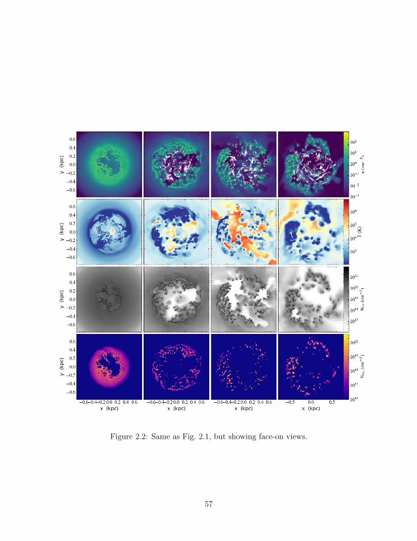
Figure 2.2: Same as Fig. 2.1, but showing face-on views.
57

Figure 2.3: The total gas scale height at various times throughout the simulation. Thesetimes match the images in Figs. 2.1 and 2.2.
58

Figure 2.4: Left: The SFR and core collapse SN rate in our dwarf galaxy in 10 Myr bins.Broken portions of this histogram are time periods with no star formation or supernovae.Note that the SN rate has been scaled by a factor of 100 to fit on the same vertical axisas the SFR. Right: The evolution of the total gas mass (black), HI mass (blue), H2 mass(orange), and stellar mass (red) in the disk of our galaxy over time.
radiation feedback. For the remainder of the simulation, the H2 mass generally increases,
with small fluctuations during periods of star formation, reaching a peak mass fraction of 5%
at 500 Myr. The growth of the molecular fraction is due in part to a decline in the total gas
content of our galaxy from feedback-driven galactic winds. During these outflows, the densest
gas, the molecular gas, is preferentially retained over the more diffuse ISM. Examining the
molecular properties of the ISM in low mass dwarf galaxies in more detail is a vital avenue
of future research, as there are significant observational uncertainties in deriving H2 content
of galaxies in this low metallicity regime (Leroy et al. 2008; McQuinn et al. 2012; Amorın
et al. 2016). The molecular properties of our galaxy are discussed further in context with
other works in Section 2.5.1.
59

2.4.3 ISM Properties
Our simulations include sufficient resolution and microphysics to capture a multi-phase
medium within the ISM and halo of our simulated galaxy. We define five different gas phases
following those defined in (Draine 2011): molecular gas, cold neutral medium (CNM), warm
neutral medium (WNM), warm ionized medium (WIM), and hot ionized medium (HIM). We
emphasize that the molecular ISM phase is defined as all cells with MH2/Mgas = fH2 > 0.5,
and is thus somewhat different than simply considering the total H2 content. By this defini-
tion, although our galaxy certainly contains molecular hydrogen, molecular gas as a phase
does not exist; the peak fH2 in any single cell remains below 30%. See Appendix 2.A for a
quantitative definition of these phases. The properties of these phases are regulated by the
complex interplay between cooling, turbulence, self-gravity, and radiative and shock heating
from stellar feedback throughout the galaxy’s evolution. Here we discuss the thermodynamic
properties of the gas within the inner halo of our dwarf galaxy.
Fig. 2.5 shows the temperature-density distribution of all gas within 0.25 Rvir of the center
of the galaxy, averaged over the time period 300–350 Myr. One can readily identify the two
regimes containing most of the mass in the simulation: low density, warm gas produced
through ionization and SN heating, and cold, high density gas that makes up most of the
mass in the galaxy’s disk (see Fig. 2.6). Several notable features of the distribution include:
broad ranges of temperature even in quite dense gas, perhaps produced by photoionization
and photoelectric heating, a substantial amount of extremely cold gas below 10 K, and the
lack of well-defined thermal phases due to the complexity of both the heating and cooling in a
turbulent medium. We note that we are likely missing important physics, such as cosmic ray
heating and ionization, that would prevent the formation of the coldest gas in this diagram
(below about 10 K), but we do not expect this to significantly alter our results. Our artificial
60

temperature ceiling in diffuse gas (see Section 2.2.1) is seen clearly by the horizontal feature
in the top left. The boxed regime in the lower right corner shows our star formation density
and temperature threshold. Gas in this regime is rapidly consumed by star formation and
subsequent feedback. Given the small size of our dwarf galaxy, the total amount of mass in
this regime at any given instant can be small, but does appear in this time average.
The mass of the ISM in our dwarf galaxy is dominated by the CNM for the entirety of the
simulation, as shown in the left panel of Fig. 2.6. The mass fraction of the remaining phases
are ordered by temperature, with the WNM as the next most-significant component. The
WNM is initially comparable to the CNM, but comprises a mass fraction of about 0.1 by the
end of the run. The WIM and HIM fluctuate significantly, corresponding to fluctuations in
the SFR and associated feedback, but are subdominant throughout the simulation. During
periods of peak stellar feedback, however, the WIM can reach a mass fraction above 0.1.
Although the CNM dominates the mass fraction, it is a negligible component of the ISM
volume, which is WIM dominated. However, the large, anti-correlated fluctuations in the
WNM and HIM make these three phases often comparable. Together, these figures better
quantify the general properties observed in the panel plots in Fig. 2.1 and Fig. 2.2.
These results are in contrast with those found for the more massive dwarf galaxy modeled
by Hu et al. (2016, 2017). They find the mass and volume fraction of the ISM are nearly
entirely dominated by warm gas (defined in those works as gas with 100 K<T< 3 × 10⁴),
with cold gas having between 1 and 10% of the mass, and occupying negligible volume. Hot
gas (defined as gas with T > 3× 10⁴ K) occupies 10% of the volume, with negligible mass,
in their galaxy, while our WIM alone occupies > 50% of the volume. Our lower mass, lower
metallicity galaxy contains more cold gas (by mass fraction) and hot gas (by volume fraction)
that seen in the more massive dwarf galaxy in these works. The driver of these differences,
which are likely somewhat related to differences in the dark matter halo potential, will be
61
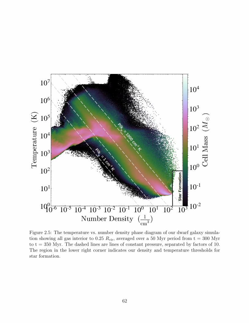
Figure 2.5: The temperature vs. number density phase diagram of our dwarf galaxy simula-tion showing all gas interior to 0.25 Rvir, averaged over a 50 Myr period from t = 300 Myrto t = 350 Myr. The dashed lines are lines of constant pressure, separated by factors of 10.The region in the lower right corner indicates our density and temperature thresholds forstar formation.
62
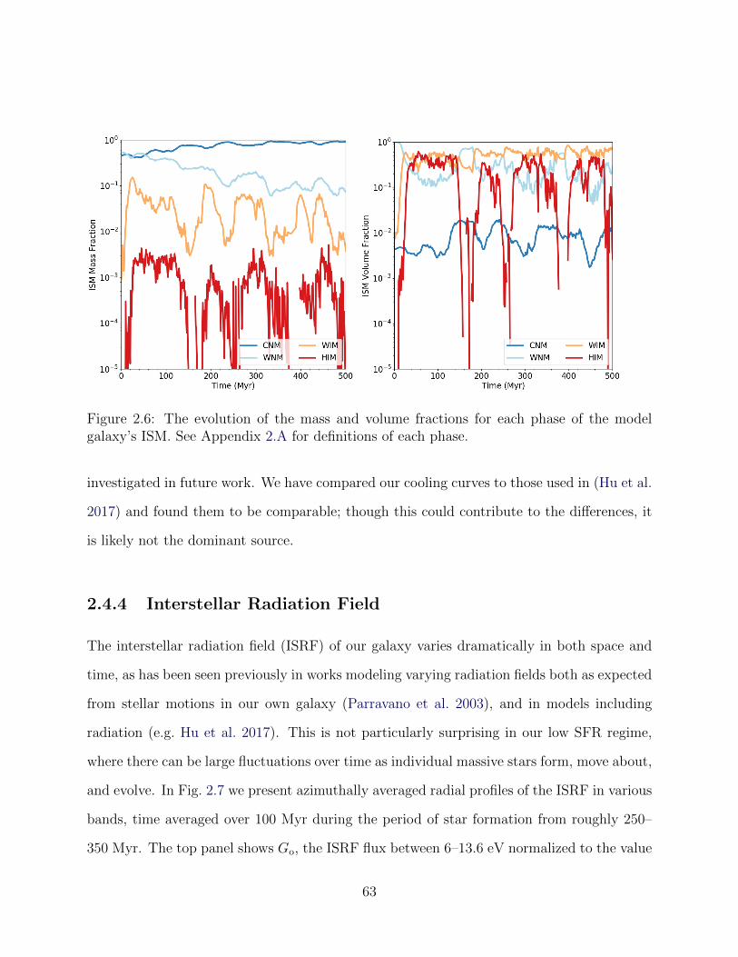
Figure 2.6: The evolution of the mass and volume fractions for each phase of the modelgalaxy’s ISM. See Appendix 2.A for definitions of each phase.
investigated in future work. We have compared our cooling curves to those used in (Hu et al.
2017) and found them to be comparable; though this could contribute to the differences, it
is likely not the dominant source.
2.4.4 Interstellar Radiation Field
The interstellar radiation field (ISRF) of our galaxy varies dramatically in both space and
time, as has been seen previously in works modeling varying radiation fields both as expected
from stellar motions in our own galaxy (Parravano et al. 2003), and in models including
radiation (e.g. Hu et al. 2017). This is not particularly surprising in our low SFR regime,
where there can be large fluctuations over time as individual massive stars form, move about,
and evolve. In Fig. 2.7 we present azimuthally averaged radial profiles of the ISRF in various
bands, time averaged over 100 Myr during the period of star formation from roughly 250–
350 Myr. The top panel shows Go, the ISRF flux between 6–13.6 eV normalized to the value
63

in the solar neighborhood of the Milky Way (see Sec. 2.2.5.6). The averaged profile varies
between values of 0.02 and 0.1, with peaks located at radii of the few active star formation
regions. At any given radius, there is over a two order magnitude variation in the ISRF
during this period of time.
The bottom panel gives the HI ionizing photon flux from stellar radiation. The ionizing
radiation profile follows a similar trend, yet with significantly more variation, anywhere from
two to four orders of magnitude. As this radiation is followed through radiative transfer, the
profile encodes information about local attenuation by dense, neutral gas. This is the main
driver of the differences between the two panels. The total fluctuation in both panels is due
in part to the low-level, stochastic star formation in our galaxy. A higher star formation
rate would produce a more regular population of massive stars and more uniform (in time)
ISRF.
To further quantify the local variations in these radiation fields, we present the full
distribution of Go and the HI ionizing flux in Fig. 2.8 at a single snapshot at 300 Myr. This
diagram shows how dramatic the increase in ISRF near young, massive stars is (the spikes in
both diagrams), while much of the mid-plane sees an ISRF orders of magnitude lower. The
striking contrast between the two diagrams is due to the shielding of the HI ionizing flux
in the most massive (cold and dense) regions of the galaxy through the radiative transfer
calculations; shielding of the FUV radiation is approximate and in general weaker, making
these regions more prominent in the left hand figure (the pink/white clumps). From both of
these diagrams, it is clear that the ISRF of a low mass dwarf galaxy varies greatly over time
and space in a way that cannot be appropriately captured by an analytic profile. Although
one could adopt an averaged radial profile to provide a realistic, global source of energy for
thermal pressure support of the gas against collapse, it is unclear how sufficient this would
be in suppressing star formation. In particular, the large increases around sites of recent star
64
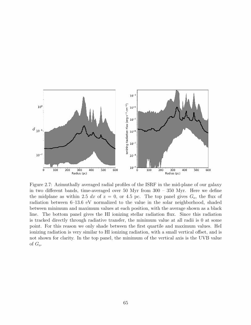
Figure 2.7: Azimuthally averaged radial profiles of the ISRF in the mid-plane of our galaxyin two different bands, time-averaged over 50 Myr from 300 – 350 Myr. Here we definethe midplane as within 2.5 dx of z = 0, or 4.5 pc. The top panel gives Go, the flux ofradiation between 6–13.6 eV normalized to the value in the solar neighborhood, shadedbetween minimum and maximum values at each position, with the average shown as a blackline. The bottom panel gives the HI ionizing stellar radiation flux. Since this radiationis tracked directly through radiative transfer, the minimum value at all radii is 0 at somepoint. For this reason we only shade between the first quartile and maximum values. HeIionizing radiation is very similar to HI ionizing radiation, with a small vertical offset, and isnot shown for clarity. In the top panel, the minimum of the vertical axis is the UVB valueof Go.
65

Figure 2.8: Single-snapshot 2D radial profile plots at 300 Myr of the ISRF in two flux bands,Go and HI ionizing radiation, illustrating the full dynamic range of radiation flux at a givenradius in the galaxy. Here, we include all gas within the mid-plane of our dwarf galaxy.Since a majority of the mass of the galaxy is in the cold phase (see Fig. 2.5), and is thereforeoptically thick to HI ionizing radiation, it does not show up in the HI ionizing radiationdiagram. This gas readily appears in the Go diagram since we assume it to be optically thin,though we do apply a localized shielding approximation.
66

formation could be important sources of feedback to destroy molecular clouds and reduce
their effective star formation efficiency. It remains to be seen which of these two modes of
feedback is more important in regulating star formation.
2.4.5 Outflow Properties
The recent FIRE cosmological simulations of dwarf galaxies over a range of dark matter halo
masses find that they exhibit large outflows, with mass loading factors (η = Mout/ < SFR >)
on order of 100–1000 (Muratov et al. 2015). However, comparable models of idealized dwarf
galaxies with detailed feedback and physics treatments find more modest mass loading factors
(Hu et al. 2016, 2017). In Fig. 2.9 we present the mass outflow and mass loading rates for
our dwarf galaxy as a function of time, computed at five different positions from the galaxy.
We follow Muratov et al. (2015) in defining the mass outflow rate at any given radius to be
the sum of the outflow rate in all cells in a spherical annulus of width dL centered at that
radius,
Mout =∑
Mgas × vr/dL. (2.7)
We choose dL = 0.1 Rvir, or 2.74 kpc.
The total mass outflow rates and mass loading factors at 0.1, 0.25, 0.5, and 1.0 Rvir are
shown in Fig. 2.9. Generally, other works use gigayear timescale measurements of the SFR
to compute the mass loading factor. For consistency with those works, we use the 500 Myr
average SFR for computing the mass loading factor. The outflow rate at 0.1 Rvir is high,
corresponding to mass loading factors between 20–100 throughout the simulation time. This
declines towards larger radii, however, with substantially less outflow past the virial radius.
Muratov et al. (2015) finds typical mass loading factors at 0.25 Rvir on order of 20–40 for
galaxies with vc = 30 km s−1 at low redshift, consistent with our results. The fluctuations
67
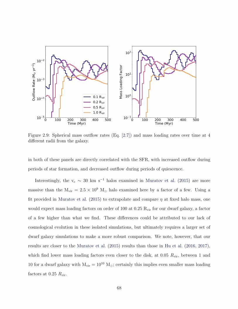
Figure 2.9: Spherical mass outflow rates (Eq. [2.7]) and mass loading rates over time at 4different radii from the galaxy.
in both of these panels are directly correlated with the SFR, with increased outflow during
periods of star formation, and decreased outflow during periods of quiescence.
Interestingly, the vc ∼ 30 km s−1 halos examined in Muratov et al. (2015) are more
massive than the Mvir = 2.5 × 10⁹ M� halo examined here by a factor of a few. Using a
fit provided in Muratov et al. (2015) to extrapolate and compare η at fixed halo mass, one
would expect mass loading factors on order of 100 at 0.25 Rvir for our dwarf galaxy, a factor
of a few higher than what we find. These differences could be attributed to our lack of
cosmological evolution in these isolated simulations, but ultimately requires a larger set of
dwarf galaxy simulations to make a more robust comparison. We note, however, that our
results are closer to the Muratov et al. (2015) results than those in Hu et al. (2016, 2017),
which find lower mass loading factors even closer to the disk, at 0.05 Rvir, between 1 and
10 for a dwarf galaxy with Mvir = 1010 M�; certainly this implies even smaller mass loading
factors at 0.25 Rvir.
68

Detailed outflow properties, beyond outflow rates and mass loading factors, can help
discriminate between the model dependent feedback physics included in galaxy simulations.
In Fig. 2.10 we present radial velocity distributions of all material outside our dwarf galaxy’s
disk, and within the halo, broken into three gas phases. Gas with a negative velocity is
moving towards the center of the halo. Roughly 25% of this mass is inflowing, mostly with
modest negative velocities, and corresponds to previously ejected gas mixing and recycling
throughout the halo. Half of the outflowing gas (positive velocities) is moving at velocities
below 30 km s−1, 75% at velocities below 70 km s−1, and 95% at velocities below 100 km s−1.
Although the mass contained in the tails of these distributions is a sub-dominant fraction of
the total, there is still a non-negligible amount of gas moving at velocities of a few hundreds
of km/s, with a peak velocity of over 700 km s−1. The WNM and WIM together dominate
the mass of both the inflowing and outflowing gas, with the WIM and HIM dominating at
velocities above 200 km s−1. The dominant launching mechanism in this simulation is SN
feedback, which generates a rapidly moving and volume-filling WIM and HIM, consistent
with the results in Hu et al. (2016, 2017). However, as shown, the HIM, which is mostly
the SN ejecta itself, comprises very little of the outflow by mass. Most of the outflowing
gas (by mass) comes from the warm phase, pushed out by the high pressure, fast moving
HIM. Some of this warm gas certainly originates from adiabatically and radiatively cooled
HIM, however. The amount of transfer between phases in the halo of our galaxy will be
investigated in future work.
69

Figure 2.10: The time averaged radial velocity distribution of outflowing material externalto the disk and within the virial radius of our dwarf galaxy. This is averaged over the sametime interval as Fig. 2.7. The outflowing material is multiphase, broken into WNM, WIM,and HIM. See Section 2.4.3 for definitions of these regimes. We note that WNM is oftenlabeled simply as “cold”, or gas below T = 104 K. There is little to no outflowing mass inthe CNM.
70
2.4.6 Metal Evolution
2.4.6.1 Metal Enriched Outflows
Dwarf galaxies efficiently, and preferentially, eject metals released in stellar feedback from
their shallow potential wells (Mac Low & Ferrara 1999; Ferrara & Tolstoy 2000). This has
been better quantified recently both observationally (e.g. Kirby et al. 2011b; Zahid et al. 2012;
Peeples et al. 2014; McQuinn et al. 2015b) and with more detailed cosmological simulations
(Simpson et al. 2013; Angles-Alcazar et al. 2017; Muratov et al. 2017). In the left panel of
Fig. 2.11, we give the metal mass loading factor for our galaxy over time, at the same radii
as in Fig. 2.9. The parameter used to quantify metal outflow efficiencies varies among works.
Here, we define the metal mass loading factor as the metal outflow rate divided by the metal
production rate, or
ηmetal =Mmetal
SFR× (Mmetal/M∗), (2.8)
where Mmetal is the metal mass outflow rate, Mmetal is the total mass in metals produced,
and M∗ is the total mass in stars. These metal loading factors fluctuate significantly with
the SFR, just as was shown in Fig. 2.9, reaching a minimum of about 0.05, but peaking at
around 5. On average, over the simulation time, ηmetal is below unity (around 0.5). Recent
simulations of outflows from a Milky Way type disk indicate typical ηmetal comparable to
our results, usually between 0.5 and 1 (Li et al. 2017; Fielding et al. 2017). Muratov et al.
(2017) computes a slightly different quantity for their galaxies, the normalized metal outflow
rate ηZ = Mmetal/SFR, finding values of about 0.02 at 0.25 Rvir regardless of galaxy circular
velocity. Our galaxy is consistent with this value, with an average ηZ = 0.015, fluctuating
between 0.007 and 0.02.
These large metal mass loading factors indicate that a majority of the metals produced in
71

Figure 2.11: Left: Metal mass loading factor (see Eq.[ 2.8]) at the same radii as in Fig. 2.9.This is the ratio between the metal outflow rate and the metal production rate. Right: Thefraction of metals contained in the disk, CGM, and outside the halo of our dwarf galaxy overtime. In both panels, we consider the total mass of all individually tracked metal species,which is zero at initialization, not the aggregate total metallicity field, which is non-zero atinitialization.
72
our dwarf galaxy are ejected from the disk. This is quantified in the right panel of Fig. 2.11,
where we show the mass fraction of metals in the disk, circumgalactic medium (CGM), and
outside the virial radius of our galaxy over time. After the first 20 Myr, SN-driven winds
rapidly drive out large quantities of metals from the disk and into the galaxy’s halo. This
continues throughout the simulation, with only ∼4% of produced metals residing in the disk
of the galaxy. It only takes 150 Myr for some metals to reach the virial radius of the halo,
with a steadily increasing fraction continually leaving the virial radius until about 350 Myr
where the fraction levels off to just above 50%. Likewise, the CGM metal content continually
decreases until the end of the simulation from loss through the virial radius of the halo. See
Section 2.5.1.3 for further discussion.
2.4.6.2 Differential Evolution of Elements Within the ISM
It is important to understand how metals from each source of stellar yields enrich the ISM.
Observations of more massive dwarf galaxies than those simulated here indicate fairly uniform
radial gas-phase metallicity profiles, even beyond the stellar radius (e.g. Werk et al. 2011;
Belfiore et al. 2017). This requires that metal mixing and transport occur on hundred
megayear timescales, much more rapidly than the gigayear timescale expected from assuming
transport at the cold gas sound speed. Therefore, either metals are transported first through
a hot phase with high sound speed, or through efficient turbulent mixing within the ISM
(e.g. de Avillez & Mac Low 2002a; Tassis et al. 2008; Yang & Krumholz 2012). It remains
uncertain how metal abundances vary in detail within these galaxies, beyond one-dimensional
radial profiles, and whether or not abundance distributions depend on the metal species. It
is even more unclear how metals are transported and distributed within low-mass dwarf
galaxies, which generally host too few H II regions for a detailed examination.
We demonstrate the power of our simulations, which capture a realistic ISM at high
73

Figure 2.12: Three slices in the mid-plane of our dwarf galaxy at 300 Myr after the startof star formation showing the variation in gas phase metal abundances. The left slice givesthe ratio of the abundance between N and O, normalized to the solar abundance, while thenumber density and temperature are shown on the right. In each, we mark massive starswith active stellar winds as white points and SNe and AGB-phase enrichment events thatoccurred in the preceding 5 Myr as black stars and orange diamonds respectively.
resolution with multiple feedback sources, by addressing these questions in Fig 2.12. The
left panel gives the abundance ratio of N to O throughout the ISM. The right two panels give
the slices of number density (top right) and temperature (bottom right) in the mid-plane of a
portion of our dwarf galaxy. These show regions with dense, cold gas clouds (n ∼ 100 cm−2,
T . 100 K) connected by cold filaments, warm, diffuse gas (n ∼ 0.1 cm−3, T ∼ 104 K), and
hot gas from a recent SN explosion (T ∼ 106 K).
As shown in the left panel, [N/O] varies significantly over this section of the ISM with
notable differences across the various phases and ISM structures. The hottest gas, domi-
nated by recent supernova explosions is overabundant in oxygen, relative to solar (purple).
However, the relative abundance of nitrogen increases in the WIM and WNM, being over-
74
abundant relative to solar (green).
At our adopted metallicity, nitrogen is predominantly produced in AGB star winds, with
very little production in core collapse SNe and winds from more massive stars. Therefore,
nitrogen is injected into the ISM with significantly less energy (v ∼ 10 km s−1) than elements
produced in SNe, like oxygen, (v ∼ 103 km s−1). Given the variations in Fig. 2.12, the
energetic differences between injection sources can drive abundance variations within the
ISM of our dwarf galaxy. The regions most rich in N are sites of recent AGB winds that
have yet to mix with the rest of the ISM. This suggests that metal mixing within the ISM
(and also metal ejection from the ISM) is species dependent. A more detailed analysis is
beyond the scope of this work, but we investigate this in detail in Emerick et al. (2018b).
2.5 Discussion
2.5.1 Comparison to Observed Low Mass Dwarf Galaxies
As noted in Section 2.3, our galaxy model is not intended to directly reproduce the ob-
served properties of Local Group ultra-faint dwarfs. Notably, our initial conditions neglect
a pre-existing stellar population and are only followed for 500 Myr, a fraction of the age
of z = 0 dwarf galaxies. However, we can still place our model in context with observa-
tions using simple comparisons to the star formation rate (Section 2.5.1.1), molecular gas
(Section 2.5.1.2), and metal retention fraction (Section 2.5.1.3) properties of observed dwarf
galaxies. We show that these properties are broadly consistent with observations.
2.5.1.1 Gas and Star Formation
The observational sample of isolated, gaseous, low mass dwarf galaxies is limited compared
to more massive galaxies, but has improved substantially with recent blind and targeted HI
75

surveys (e.g. Giovanelli et al. 2005; Geha et al. 2006, 2012; Walter et al. 2008; Cannon et al.
2011; Haynes et al. 2011; Hunter et al. 2012; Bradford et al. 2015; James et al. 2015; Tollerud
et al. 2015; Sand et al. 2015; Wang et al. 2017). However, the sample of isolated, gaseous
dwarf galaxies with M∗ < 107 M� remains small. In Figure 2.13 we show where our galaxy
lies relative to the observed Kennicutt-Schmidt relation and extended Schmidt law for low
mass galaxies. In both diagrams, our simulations are given by the colored points, sampled
every megayear throughout the entire simulation.
Although simple to measure in simulations, these quantities are challenging to directly
compare to observations. We have attempted to make a reasonable analog to how Σsfr and
Σgas are measured observationally for low mass dwarfs (see Roychowdhury et al. 2014). We
define Σsfr = M∗,10/A∗,10, where M∗,10 is the SFR measured over the preceding 10 Myr, and
A∗,10 is the area of the disk within the radius of the outermost star formed within the previous
10 Myr. Likewise, Σgas = Mgas,10/A∗,10, where Mgas,10 is the total gas mass within this defined
disk. However, the total gas content cannot be determined observationally. To match this
limitation, we follow Roychowdhury et al. (2014) and take Σgas,obs = 1.34 × ΣHI, where the
factor 1.34 attempts to account for He. We note that there is generally no correction made
for any possible H2 or HII content. As shown in Section 2.5.1.2, these components may be
significant.
We include recent observational constraints on these relationships in Figure 2.13. Our
galaxy fluctuates significantly about both relationships with no clear trends in time. How-
ever, in both cases, it is consistent with the available observational sample. At times our
galaxy exhibits gas surface densities below the observational constraints. The trend is still
consistent with higher densities at this point, but with a larger scatter towards lower star
formation rate densities and efficiencies.
In constructing our galaxy model, we employed no tuning of the underlying physics,
76
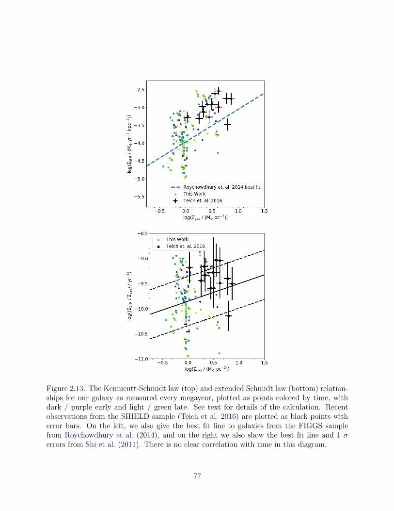
Figure 2.13: The Kennicutt-Schmidt law (top) and extended Schmidt law (bottom) relation-ships for our galaxy as measured every megayear, plotted as points colored by time, withdark / purple early and light / green late. See text for details of the calculation. Recentobservations from the SHIELD sample (Teich et al. 2016) are plotted as black points witherror bars. On the left, we also give the best fit line to galaxies from the FIGGS samplefrom Roychowdhury et al. (2014), and on the right we also show the best fit line and 1 σerrors from Shi et al. (2011). There is no clear correlation with time in this diagram.
77
adopting only canonical values for any available free parameters. It is thus non-trivial that
our galaxy should oscillate about the median relationships in Fig. 2.13, and signifies a proper
accounting of the relevant physics governing gas and star forming properties in our galaxy.
This result is consistent with galactic evolution simulations run at high resolution with a
detailed accounting of stellar feedback physics (see Naab & Ostriker 2017, and references
therein) and with the demonstration by Li et al. (2005) that the Kennicutt-Schmidt law can
be reproduced by gravitation acting on an isothermal disk. The net result of the complex
interactions of heating, cooling, chemistry, and feedback physics on star formation is to offset
to a level not too dissimilar to more simple simulations considering gravity alone.
2.5.1.2 Molecular Gas Content
The molecular gas content of low-mass dwarf galaxies is generally assumed to be small, but
is not well constrained by either theory or observations. Assuming the relationship in Leroy
et al. (2013) and Momose et al. (2013), Roychowdhury et al. (2014) finds typical molecular
gas mass fractions can be anywhere from fH2 = 0.05 to fH2 = 0.5; a significant range in
values. As discussed in Section 2.2.4, our galaxy has fH2 of 0.001 – 0.05, just overlapping
with this range. H2 formation in our model is possible through formation on dust, the three
body interaction, or the gas-phase reaction H− + H → H2 + e−. The gas-phase reaction
dominates in our low-metallicity galaxy over the other two channels by several orders of
magnitude. In our model, H− is produced solely through the reaction H + e− → H− + γ.
Thus the presence of some ionizing background is required to generate the molecular fractions
we find in our simulations, as confirmed in separate test simulations.
In contrast, Hu et al. (2016) and Hu et al. (2017) find low molecular fractions (fH2 ∼ 10−4)
even in their simulations without any feedback (fH2 ∼ 2 × 10⁻³). However, although these
works do contain a non-equilibrium chemical model, they do not include either H− or a
78

background radiation field. Our model suggests that both H− and the UV background are
critical components in H2 formation in small dwarf galaxies. Indeed it is not surprising that
the gas phase reactions dominate over grain catalysis at low metallicity (Glover 2003), though
it is worth noting that the rate coefficients associated with gas-phase H2 formation are still
uncertain by an order of magnitude (Glover et al. 2006; Glover & Mac Low 2007). Our model
does lack additional chemistry that may be important to the formation and destruction of
H2, including HD chemistry, C and O chemistry, a detailed dust model, and cosmic rays.
In addition, our model does not account for the stellar component of the radiation field
that leads to H− photodetachment (Eγ > 0.76 eV), though we do account for the contribution
from the UVB. We find that the H2 fraction is more strongly dependent upon the Lyman-
Werner radiation field, which is followed for each star, than the H− photodetachment rate.
Our tests suggest that, by ignoring the stellar contribution to H− photodetachment, our
results may represent upper limits on the H2 mass. However, including this component will
likely only make a substantial difference during periods of no star formation, when there
are no massive stars with significant Lyman-Werner luminosities. We do not anticipate this
to have a significant dynamical impact on our simulations, as is discussed in more detail in
Appendix 2.E.
It is unclear how the combination of all of the above effects will behave, especially con-
sidering that, even at this resolution, we are unable to resolve the high density turbulent
density perturbations in which H2 forms most efficiently (Glover & Mac Low 2007). These
uncertainties certainly warrant further study of molecular gas in low metallicity dwarf galax-
ies.
79
2.5.1.3 Metal Retention
The simulations presented here have not yet been run for the gigayear timescales required
to begin to make direct comparisons to the observed stellar and gas phase metallicities of
comparable dwarf galaxies at z = 0. However, we can compare to a key observable: the
retention fraction of metals within stars and the galaxy’s ISM compared to what would be
expected from closed box stellar evolution models given the galaxy’s star formation history.
This can be done readily with Milky Way dSph’s. Their stars seem to retain very little of
the expected metal production: on order of a few percent or less depending on the galaxy
and the species (Kirby et al. 2011b). However, environmental effects, namely ram pressure
and tidal stripping, complicate the understanding of how these metals were removed from
the galaxy.
Leo P, the dwarf galaxy we approximate in our initial conditions, is extremely valuable
as a gas-rich, star forming, low-mass dwarf galaxy, with an observable HII region, necessary
for determining gas phase abundances, that is close enough to the Milky Way to conduct
this experiment. Leo P retains ∼ 5% ± 2% of its metals, ∼ 1% in stars and the rest in ISM
gas (McQuinn et al. 2015b). As discussed in Section 2.4.6, more than 90% of the tracked
metals produced during our simulation no longer reside within the galaxy’s disk, agreeing
with observations. However, this is an evolving quantity that also depends on how much
(if any) subsequent re-accretion of these metals occurs. Although more than half of these
metals are expected to eventually re-accrete (Christensen et al. 2016, 2018; Angles-Alcazar
et al. 2017), it is still possible that most of the metals that have been produced at these
early times will remain outside the galaxy disk.
It is interesting to consider whether ejected metals in our model reside in the CGM or
have been ejected into the intergalactic medium. While this is very challenging to determine
80
observationally for dwarf galaxies at this mass, cosmological simulations of an Mvir = 1010
M� galaxy show that, by redshift zero 40% is ejected from the galaxy’s halo (Angles-Alcazar
et al. 2017). We find 5.3% of all metals lie within 1 kpc of the center of our galaxy, 24.5%
within 0.25 Rvir (or 6.85 kpc), and 51% outside Rvir. This is consistent with previous works,
but this is again an evolving quantity. In addition, the amount of gas that escapes the virial
radius is certainly sensitive to the details of gas accretion from the IGM on this galaxy, which
we cannot capture in this model.
The re-accretion or final ejection of this gas is directly relevant to the chemical evolution
of low mass dwarf galaxies. Recycling of metal enriched gas could be a significant driver of
long-term chemical evolution in low mass galaxies, particularly if a majority of metals ejected
from the disk (itself nearly all the metals produced by the galaxy) return. In addition, the
accretion of pristine gas from the intergalactic medium could significantly affect the gas
flows around the galaxy, possibly promoting the retention of ejected metals. This effect is
not included in our isolated galaxy simulations, and its role is beyond the scope of this work.
2.5.2 Missing Physics
Although we include many detailed physical models in our simulations, there remain addi-
tional physical processes that may be relevant, which we now discuss.
2.5.2.1 Massive Stellar Wind Energy
Our massive stellar wind model drastically reduces the injected wind velocity from∼1000 km s−1
to 20 km s−1. Although our algorithm is entirely capable of generating realistic stellar winds
with velocities comparable to those observed, such fast winds place a near constant and
severe constraint on the Courant time step that renders &100 Myr simulations impractical.
When considered in isolation, stellar winds are an important source of pre-SN feedback and
81
can dramatically influence dynamical evolution on molecular cloud and galaxy scales (Dale
& Bonnell 2008; Peters et al. 2017; Gatto et al. 2017). However, when considered together
with ionizing radiation, stellar winds contain less total energy (Agertz et al. 2013) and do
not seem to have a significant dynamical influence in either idealized simulations (Geen et al.
2015) or individual giant molecular clouds (Dale et al. 2014), unless densities near the ion-
izing source are high enough to trap the HII region in the source cell. In that case, they can
clear out a cavity to allow initial establishment of the HII region.
They are even less relevant in the low-metallicity regime studied here, as stellar winds
become weaker with decreasing metallicity (Puls et al. 2000; Vink & de Koter 2005). Al-
though they likely have minimal dynamical importance at resolutions where peak densities
are not anyway high enough to trap ionization fronts, a full model of stellar winds may affect
detailed ISM properties and metal mixing, warranting closer examination in future work.
2.5.2.2 Cosmic Rays
Recent work has explored the importance of cosmic ray feedback in regulating the ISM and
wind properties in galactic disks (Hanasz et al. 2013; Girichidis et al. 2016; Simpson et al.
2016; Farber et al. 2018), isolated galaxies (Salem et al. 2016, 2015; Pakmor et al. 2016;
Ruszkowski et al. 2017), and galaxies in cosmological context (Salem et al. 2014). These
relativistic charged particles act as a source of non-thermal pressure support in the galaxy’s
ISM, capable of driving outflows at different velocities and containing different thermal
phases than those driven through thermal feedback alone (Salem et al. 2016). Modeling
cosmic rays is challenging, however, as they encompass a wide range of energies, and there
are significant uncertainties in how they propagate through the ISM (e.g. Wiener et al.
2017). Their propagation is often modeled as a diffusive process, but in truth this diffusion
should vary depending on cosmic ray energy. In addition, cosmic rays couple effectively to
82

the magnetic fields of galaxies, diffusing preferentially along structured magnetic field lines
within the ISM. Modeling cosmic ray feedback completely thus requires both an accurate
cosmic ray model and magnetohydrodynamics in order to capture the interplay of these two
physical phenomena. Finally, including MHD presents additional difficulties in untangling
the effects of each individual feedback mechanism on galaxy chemodynamics.
We do note that an isotropic, two-fluid model for cosmic ray feedback exists in Enzo
(Salem & Bryan 2014; Salem et al. 2015) and has been well tested. Mechanically, including
this relatively simple treatment of cosmic ray feedback in our model is trivial. However,
the cosmic ray population, their diffusion coefficient, and the magnetic field structure of the
lowest mass dwarf galaxies each have significant enough uncertainties to warrant reserving
their full inclusion into our model to later work.
2.5.3 Detailed Stellar Evolution and Binary Stars
Roughly half of massive stars live in binary pairs (Sana et al. 2013). Their interactions,
primarily through mass transfer, can significantly alter their radiation properties and life-
times. This can change both how much and how long these stars emit ionizing radiation, an
important source of stellar feedback, and where and when these stars explode as SNe. This
effect could be significant, but is rarely accounted for in galaxy evolution models, which
are commonly based on calculations of single star evolution (e.g. STARBURST99). For
example, Zapartas et al. (2017) finds that binarity extends the timescales over which core
collapse SNe occur from a given star formation event, from a maximum time of ∼ 50 Myr to
∼ 200 Myr. Although they find only ∼ 15% of core collapse SNe explode after 50 Myr, this
could still be an important effect. Properly accounting for the delay times due to variations
in individual star lifetimes has already been shown to change the significance of feedback and
influence galaxy metallicity properties (Kimm et al. 2015). Extending the lifetimes of these
83
stars combined with accounting for binary effects that change the luminosities of these stars
(Gotberg et al. 2017, 2018) could increase the importance of radiation feedback; however
this may be less important as these additional photons are more likely to escape the galaxy
(e.g. Ma et al. 2016b).
Since we model stars on a star-by-star basis, both of these effects could be reasonably
accounted for by stochastically assigning binary star properties to some subset of our in-
dividual stars. This is beyond the scope of this project, but will be investigated in future
work.
2.6 Conclusion
We have developed a new method for simulating galaxy evolution with detailed feedback and
chemical enrichment. For the first time on galaxy scales, we simultaneously model multi-
channel stellar feedback in detail, using individual star particles to model core collapse and
Type Ia SNe, ionizing radiation followed through radiative transfer, photoelectric heating,
Lyman-Werner radiation and pollution from AGB and massive stellar winds. This treatment
of feedback, coupled with the detailed chemistry and heating/cooling physics followed with
Grackle, allows us to capture realistic galaxy evolution in detail. In this work, we apply
these methods to simulate the evolution of an isolated, low-mass, dwarf galaxy modeled after
the z = 0 properties of the Leo P dwarf galaxy. We present an overview of the properties of
this simulation in this work.
For our simulated dwarf galaxy, we find:
1. Multi-channel feedback is effective in regulating star formation to a rate consistent
with the Kennicutt-Schmidt relationship and the extended Schmidt law in observed
galaxies. (See Figs. 2.4 and 2.13).
84

2. This feedback drives large outflows having mass loading factors of η ∼ 50 at 0.25 Rvir,
falling to η ∼ 10 at Rvir, and metal mass loading factors near unity. By mass, nearly
all of this outflow is moving with velocities below 100 km s−1, but there is a significant
tail towards velocities up to 1000 km s−1 (See Fig. 2.10).
3. Only ∼4% of metals are retained in the disk of our simulated galaxy, consistent with
the observed metal retention fractions of low-mass dwarfs. By the end of the simulation
∼45% of the remaining metals stay within the virial radius (but outside the galaxy),
while ∼50% have been ejected beyond the virial radius. (See Figs. 2.9, 2.10, and 2.11.)
4. Beyond the stellar radius, the gas scale height is thin (∼ 50 pc), yet resolved, with
larger scale heights (∼ 100–200 pc) driven by feedback interior to the stellar radius.
This is comparable to the resolution limit of the diffuse HI in observed, gaseous low-
mass dwarfs. At a spatial resolution of 100 pc, our galaxy has a peak HI column
density NHI = 2.8− 4.3× 1020 cm−2, depending on inclination (See Fig. 2.3).
5. The ISRF of our galaxy varies strongly in both space and time by orders of magnitude.
It is unclear how important these fluctuations are as a source of feedback, or if the affect
can be approximated with a time-averaged radial profile. The importance of radiation
feedback in our model is investigated in more detail in Emerick et al. (2018b). (See
Figs. 2.7 and 2.8.)
6. We find H2 fractions below 5% in our dwarf galaxy, consistent with the poor constraints
on molecular gas formation in low metallicity dwarf galaxies. This H2 forms entirely
through gas-phase reactions facilitated by H− in self-shielding regions; H2 formation
on dust grains and in the three body reaction are both insignificant. Cold, neutral
hydrogen dominates the mass of our galaxy. While warm, neutral hydrogen is present,
it does not dominate the mass fraction (See Fig. 2.4 and Fig. 2.6.)
85
7. Finally, we present gas-phase oxygen and nitrogen distributions as examples to briefly
demonstrate that there are marked differences in how individual metal species are
distributed within the ISM of our galaxy. These variations could be tied to differences
in elemental yields among different sources (for example, AGB winds vs. SNe), as
suggested by Krumholz & Ting (2018). This is explored in more detail in (Emerick
et al. 2018b).
Acknowledgments:
We would like to thank the following for their advice and valuable discussions, without
which this work would not have been possible: B. Cote, S. Glover, K. Hawkins, C. Hu, K.
Johnston, B. O’Shea, M. Putman, B. Smith, J. Wall, and J. Wise. We would additionally like
to thank the referee for their careful report. A.E. is funded by the NSF Graduate Research
Fellowship DGE 16-44869. G.L.B. is funded by NSF AST-1312888, NASA NNX15AB20G,
and NSF AST-1615955. M.-M.M.L. was partly funded by NASA grant NNX14AP27G. We
gratefully recognize computational resources provided by NSF XSEDE through grant number
TGMCA99S024, the NASA High-End Computing Program through the NASA Advanced
Supercomputing Division at Ames Research Center, Columbia University, and the Flatiron
Institute. This work made significant use of many open source software packages, including
yt, Enzo, Grackle, Python, IPython, NumPy, SciPy, Matplotlib, HDF5, h5py,
Astropy, Cloudy and deepdish. These are products of collaborative effort by many
independent developers from numerous institutions around the world. Their commitment to
open science has helped make this work possible.
86
2.A Gas Phases of the ISM
To aid in comparison to other works, we define our ISM phases here, as adopted and modified
from Draine (2011), Table 1.3, and used consistently throughout this analysis. By construc-
tion, these phases are mutually exclusive. We take fH2 to be the molecular hydrogen fraction
of the total gas mass.
1. Hot Ionized Medium (HIM): T ≥ 105.5 K
2. Warm Ionized Medium (WIM): 104 K ≤ T < 105.5 K
3. Warm Neutral Medium (WNM): 102 K ≤ T < 104 K
4. Cold Neutral Medium (CNM): T < 102 K, fH2 ≤ 0.5
5. Molecular: T < 102 K, fH2 > 0.5
2.B Stellar Radiation Properties
We determine the radiation properties of our model stars as a function of stellar mass and
metallicity from the OSTAR2002 grid (Lanz & Hubeny 2003) in the regime that it covers, or
integrated from an adjusted black body curve for other stars, given the ZAMS stellar radius
obtained from the PARSEC (Bressan et al. 2012; Tang et al. 2014) stellar evolution data
set. In Fig. 2.B.1 we plot these properties. We use a constant factor across metallicities for
stars not sampled on the OSTAR2002 grid to shift the black body radiation fluxes to be
roughly continuous with the ionizing photon rates and luminosities as a function of stellar
mass. This requires two factors for each radiation type, one for low mass and one for high
mass stars. We use the following multiplicative factors to adjust the black body spectrum
87

for HI and HeI ionizing radiation respectively: [0.1, 3.2] and [0.0001, 4.0]. We do not find
this adjustment to be necessary for the FUV and Lyman-Werner radiation bands.
The ionizing radiation photon energies are taken as the average ionizing photon energy
for a black body of the star’s given Teff obtained from the PARSEC grid. A more accurate
approach to compute this energy would convolve the full stellar spectrum and the frequency-
dependent absorption cross section. We tested this approach using the frequency-dependent
photoionization cross sections from Verner et al. (1996).10 The blackbody approximation
is accurate to within 5%, yet substantially easier to compute on the fly, as integrals over
the blackbody spectrum can be expressed as infinite series that rapidly converge to high
precision. Unlike for the ionizing radiation, we assume constant FUV and Lyman-Werner
band energies for each star, at 9.8 eV and 12.8 eV respectively.
2.C Typical Gas Densities in Supernova Injection Re-
gions
Modeling SN feedback with the injection of thermal energy alone can lead to rapid overcooling
of the injected energy, and a significant underestimate of the effects of SN feedback. Often,
ad hoc solutions to this problem are used in large simulations with coarse resolution, such as
momentarily turning off cooling in feedback affected regions or decoupling affected regions
from the hydrodynamics for some time. However, physically consistent solutions have been
developed (e.g Simpson et al. 2016) that inject a mixture of kinetic and thermal energy
with a ratio that depends on resolution and local gas density. Overcooling becomes less
important with higher resolution and lower ISM densities, until eventually pure thermal
10Source code containing the analytic fits given in Verner et al. (1996) was obtained from http://www.
pa.uky.edu/~verner/photo.html
88

Figure 2.B.1: Radiation properties for our model stars, showing the ionizing photon lu-minosities for HI (top left) and HeI (top right) for each star, the FUV (middle left) andLyman-Werner (middle right) luminosities, and finally the average ionizing photon energyfor HI (bottom left) and HeI (bottom right). Note, we only track radiation from stars above8.0 M�, which dominate over less massive stars, even when accounting for IMF weighting.
89
energy injection is sufficient to resolve each SN. We take advantage of our high resolution
and employ a simple thermal energy injection model for our SN feedback. We demonstrate
how well this resolves our SNe in the comparison simulation presented in this work.
The left panel of Fig. 2.C.1 gives the distributions of the peak and average ISM number
densities in the SN injection regions for each SN in our fiducial simulation. As shown, a
majority explode in regions at substantially lower densities than the star formation threshold
of 200 cm−3. For most SNe, nmax ≤ 1.0 cm−3, which is due to the substantial pre-SN feedback
included in our simulations. The right panel of Figure 2.C.1 gives the fractional distribution
of the calculated radius of the pressure-driven snowplow (RPDS) phase of the Sedov-Taylor
expansion, adopting the definitions from Simpson et al. (2016)
RPDS =
49.3E
1/451 n
−1/2o ifZ ≤ 0.01
18.5E2/751 n
−3/7o Z−1/7 ifZ ≥ 0.01
(2.9)
where E51 is the injection energy in units of 1051 erg, no is the number density of the medium,
and Z is the metallicity in units of Zo. Simpson et al. (2016) found that RPDS > 4.5∆x is
needed to resolve the SN explosion with thermal energy injection alone, assuming uniform
density in the injection region. In practice, the injection region is never uniform. We give
RPDS assuming uniform density at both the average and maximum number density in the
injection region of each SN. As shown, a majority of SNe are resolved (to the right of the
4.5∆x line), but up to 8.3% are not well resolved and 2.0% are completely unresolved (below
a single cell width). In general, these are SN explosions from the most massive (i.e. most
prompt) stars. We do not expect that resolving these SNe will dramatically alter our results.
However, we note that using our feedback model at resolutions much less than a few parsecs
will require implementing an different injection mechanism.
90
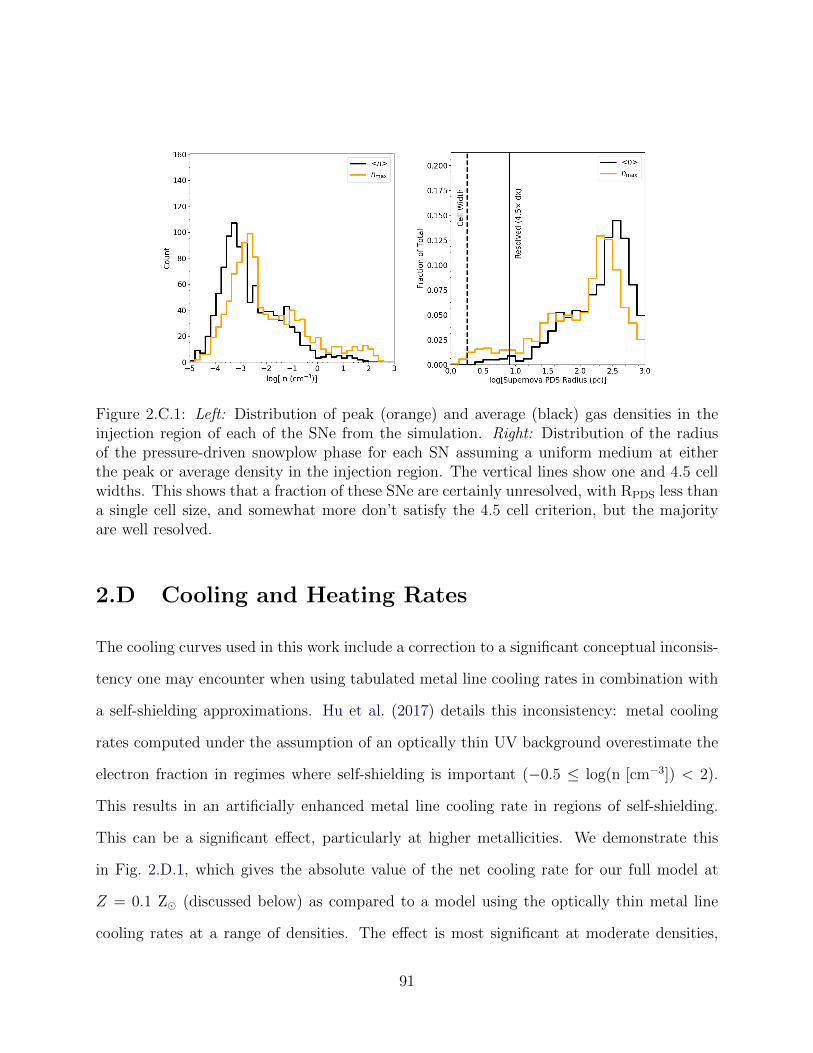
Figure 2.C.1: Left: Distribution of peak (orange) and average (black) gas densities in theinjection region of each of the SNe from the simulation. Right: Distribution of the radiusof the pressure-driven snowplow phase for each SN assuming a uniform medium at eitherthe peak or average density in the injection region. The vertical lines show one and 4.5 cellwidths. This shows that a fraction of these SNe are certainly unresolved, with RPDS less thana single cell size, and somewhat more don’t satisfy the 4.5 cell criterion, but the majorityare well resolved.
2.D Cooling and Heating Rates
The cooling curves used in this work include a correction to a significant conceptual inconsis-
tency one may encounter when using tabulated metal line cooling rates in combination with
a self-shielding approximations. Hu et al. (2017) details this inconsistency: metal cooling
rates computed under the assumption of an optically thin UV background overestimate the
electron fraction in regimes where self-shielding is important (−0.5 ≤ log(n [cm−3]) < 2).
This results in an artificially enhanced metal line cooling rate in regions of self-shielding.
This can be a significant effect, particularly at higher metallicities. We demonstrate this
in Fig. 2.D.1, which gives the absolute value of the net cooling rate for our full model at
Z = 0.1 Z� (discussed below) as compared to a model using the optically thin metal line
cooling rates at a range of densities. The effect is most significant at moderate densities,
91
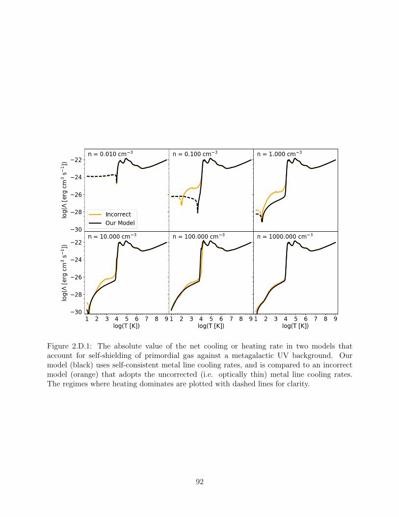
Figure 2.D.1: The absolute value of the net cooling or heating rate in two models thataccount for self-shielding of primordial gas against a metagalactic UV background. Ourmodel (black) uses self-consistent metal line cooling rates, and is compared to an incorrectmodel (orange) that adopts the uncorrected (i.e. optically thin) metal line cooling rates.The regimes where heating dominates are plotted with dashed lines for clarity.
92

where the net cooling rate can be an order of magnitude higher. In low temperature regions,
this can significantly shift the inferred equilibrium temperature and reduce the cooling time
of dense gas. Fig. 2.D.2 shows the net cooling rate and the individual heating and cooling
rates from our generated tables at low metallicity, Z = 0.01 Z�, comparable to that used in
our dwarf galaxy. We have made these tables publicly available in the main distribution of
Grackle and discuss how they were generated below.
For densities where self-shielding is important, we computed Cloudy models of one-
dimensional clouds at each temperature and density pair with a physical size corresponding
to the Jeans length. In cases where the Jeans length is very large, we limit the size to 100
pc, a reasonable approximation for the maximum size of a self-gravitating cloud. We then
adopt the metal line cooling rates obtained from the center of these clouds, whose outside is
exposed to the UV background. These models were computed with a modified version of the
CIAOLoop11 code used in Smith et al. (2008). In computing these tables we had to include the
cosmic ray ionization that dominates in optically thick clouds. Without this effect, Cloudy
becomes unstable in entirely neutral regions. We adopted a cosmic ray ionization rate of
10% the Milky Way value, though we note that varying this from 1% to 100% the Milky
Way value did not have an effect on the extracted metal line cooling rates.
Finally, we note that the cooling and heating rates in our simulation will deviate from
these curves, as they depend upon local conditions that cannot be accounted for here. The
primordial cooling and heating rates are computed consistently with the non-equilibrium
chemistry solver, leading to deviations from the tabulated primordial rates, and the heating
rates depend upon the local stellar radiation field, which is not included in these diagrams.
11https://bitbucket.org/brittonsmith/cloudy cooling tools (our version: https://github.com/aemerick/cloudy tools)
93
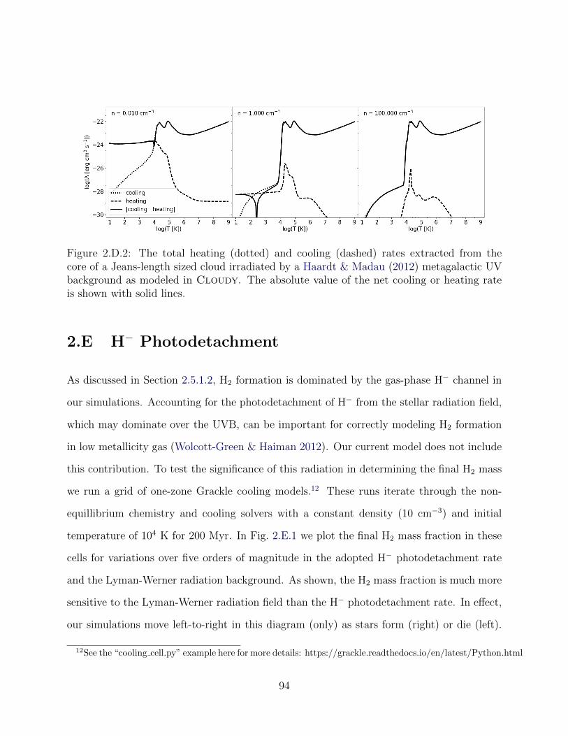
Figure 2.D.2: The total heating (dotted) and cooling (dashed) rates extracted from thecore of a Jeans-length sized cloud irradiated by a Haardt & Madau (2012) metagalactic UVbackground as modeled in Cloudy. The absolute value of the net cooling or heating rateis shown with solid lines.
2.E H− Photodetachment
As discussed in Section 2.5.1.2, H2 formation is dominated by the gas-phase H− channel in
our simulations. Accounting for the photodetachment of H− from the stellar radiation field,
which may dominate over the UVB, can be important for correctly modeling H2 formation
in low metallicity gas (Wolcott-Green & Haiman 2012). Our current model does not include
this contribution. To test the significance of this radiation in determining the final H2 mass
we run a grid of one-zone Grackle cooling models.12 These runs iterate through the non-
equillibrium chemistry and cooling solvers with a constant density (10 cm−3) and initial
temperature of 104 K for 200 Myr. In Fig. 2.E.1 we plot the final H2 mass fraction in these
cells for variations over five orders of magnitude in the adopted H− photodetachment rate
and the Lyman-Werner radiation background. As shown, the H2 mass fraction is much more
sensitive to the Lyman-Werner radiation field than the H− photodetachment rate. In effect,
our simulations move left-to-right in this diagram (only) as stars form (right) or die (left).
12See the “cooling cell.py” example here for more details: https://grackle.readthedocs.io/en/latest/Python.html
94

A complete model, including the stellar contribution to H− photodetachment, would move
somewhat diagonally.
We follow up on the qualitative conclusions of these models by running four simulations
at the four points in the diagram. These runs have identical initial conditions, random
SN driving, cooling, heating, and chemistry as our fiducial simulation, but with no star
formation. We vary the Lyman-Werner radiation and the H− photodetachment rate by the
factors shown, which are comparable to the ratio between the typical ISRF and the UVB in
the disk of our galaxy (see Fig. 2.7). Changing the background H− photodetachment rate
by a factor of 100 only (top left star) leads to a reduction in the final H2 mass fraction by
3, while changing the Lyman-Werner background by a factor of 100 (bottom right point)
decreases the H2 mass by a factor of 6.9. Applying both scale factors gives a reduction of
7.9. Thus, we see that the difference between the more realistic case in which both rates
increase by the same factor, and the case assumed in the simulations, is only about 20%.
Although the replacement of star formation by random SNe in these models produces
qualitatively different galaxy properties, the point of these simulations is to be maximal
models of H2 formation. We demonstrate that, even in this case, there is not a dramatic
change in the total H2 formation and that the effect of varying the H- photodetachment rate
is sub-dominant to other factors. Therefore, we do not expect that ignoring this component
of the stellar radiation field will have a significant dynamical impact on our galaxy evolution.
H− photodetachment arises from lower energy photons, above 0.76 eV, with a peak in
effectiveness around 2 eV. For this reason, low mass stars may contribute significantly, if
not dominate, the radiation field responsible for this reaction. The Lyman-Werner radiation
field is dominated by short-lived massive stars, with some contribution from older stars up
to a few hundred Myr, and is thus subject to significant fluctuations, particularly in periods
of no star formation. During these times, H− photodetachment from low energy photons
95
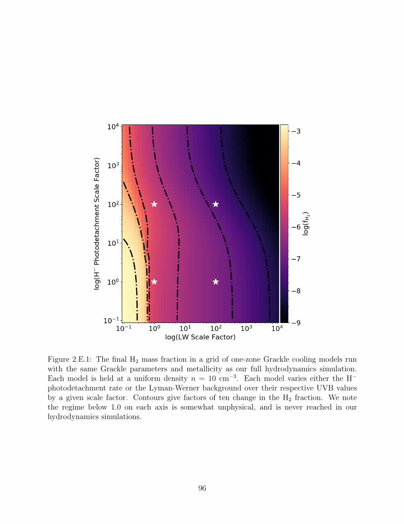
Figure 2.E.1: The final H2 mass fraction in a grid of one-zone Grackle cooling models runwith the same Grackle parameters and metallicity as our full hydrodynamics simulation.Each model is held at a uniform density n = 10 cm−3. Each model varies either the H−
photodetachment rate or the Lyman-Werner background over their respective UVB valuesby a given scale factor. Contours give factors of ten change in the H2 fraction. We notethe regime below 1.0 on each axis is somewhat unphysical, and is never reached in ourhydrodynamics simulations.
96

may play a non-negligible role in regulating H2 formation. Indeed there is H2 growth during
these periods due to a decrease in the Lyman-Werner field, but it is unclear how much of
this would be attenuated by accounting for photons from lower mass stars. Doing so in our
current model, applying an optically thin 1/R2 field for each star, would be computationally
challenging due to the dramatic increase in the number of stars whose radiation would need
to be tracked.
As emphasized in Section 2.5.1.2, further work modeling low-metallicity dwarf galaxies
with a more detailed chemistry model would be useful to clarify the role of various competing
phenomena in driving the molecular properties of these galaxies.
2.F Resolution Study
We demonstrate the effect of varying resolution in the evolution of our galaxy model in
Fig. 2.F.1. We compare the star formation rate, mass evolution, and metal ejection / re-
tention fractions between our fiducial high-resolution simulation (solid lines) with the same
simulation at two lower maximum resolutions, 3.6 pc (dashed lines), and 7.2 pc (dash-dotted
lines). The physics in each simulation remains the same with the exception of star forma-
tion, which employs a resolution-dependent density threshold. A factor of two decrease in
resolution translates to a factor of four decrease in the star formation density threshold,
from 200 cm−3 in our fiducial runs, to 50 cm−3 and 12.5 cm−3 in our 3.6 pc and 7.2 pc
resolution runs respectively. As a result, the time at which star formation first occurs varies
between the simulations, but we again define t = 0 as the time of first star formation in each
simulation.
Fig. 2.F.1 shows that, while decreasing the resolution certainly changes the evolution,
the simulations are similar to within a factor of a few. We argue that these differences
97
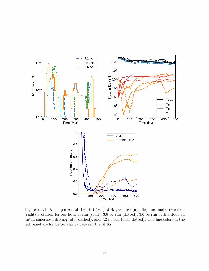
Figure 2.F.1: A comparison of the SFR (left), disk gas mass (middle), and metal retention(right) evolution for our fiducial run (solid), 3.6 pc run (dotted), 3.6 pc run with a doubledinitial supernova driving rate (dashed), and 7.2 pc run (dash-dotted). The line colors in theleft panel are for better clarity between the SFRs.
98

are within the stochastic variation one would expect from simulations with stochastic star
formation. The star formation rate and total stellar mass is correlated with resolution, with
our fiducial run having the highest SFR and stellar mass among the three runs. We note
that the self-consistent SNe are still resolved in the 3.6 pc runs since these still explode at
the low densities seen in Fig. 2.C.1. However, although feedback in general is still effective
in the 7.2 pc run, SNe are not well resolved at this resolution.
Generally ineffective feedback leads to increased, not decreased, star formation rates.
However, the lower resolution run has the lowest SFR. The source of this difference is likely
related to the ability to resolve dense, cold gas in the lower resolution simulations. In
particular, the low resolution simulation clearly is unable to resolve the densities at which
gas-phase H2 formation becomes efficient, leading to significantly lower H2 fractions (middle
panel) and lower cooling rates. In addition, whatever H2 does form at these lower resolutions
exists at lower gas densities than in our fiducial run, and is less well protected by self-shielding
effects. This is shown clearly in the significant plummet in the H2 mass during the phase
of first star formation that is less severe in our fiducial run. In this low metallicity regime,
where H2 is an important coolant, the ability to resolve the densities responsible for H2
formation and self-shielding is important.
Theses differences in densities are shown clearly by comparing Fig. 2.5 with Fig. 2.F.2.
Although the lowest temperature reached in each simulation is comparable, there is less gas in
the coldest, densest portion of the phase diagram in each of the lower resolution simulations.
In the 7.2 pc run, the gas phases are notably less distinct, with gas more evenly smoothed
out in the multi-phase region between cold, dense gas and warm, ionized gas. We note the
7.2 pc simulation, which ran quickly, was conducted without the temperature ceiling used
in the 3.6 pc and fiducial runs; we do not expect this to have a significant effect on the
comparison.
99
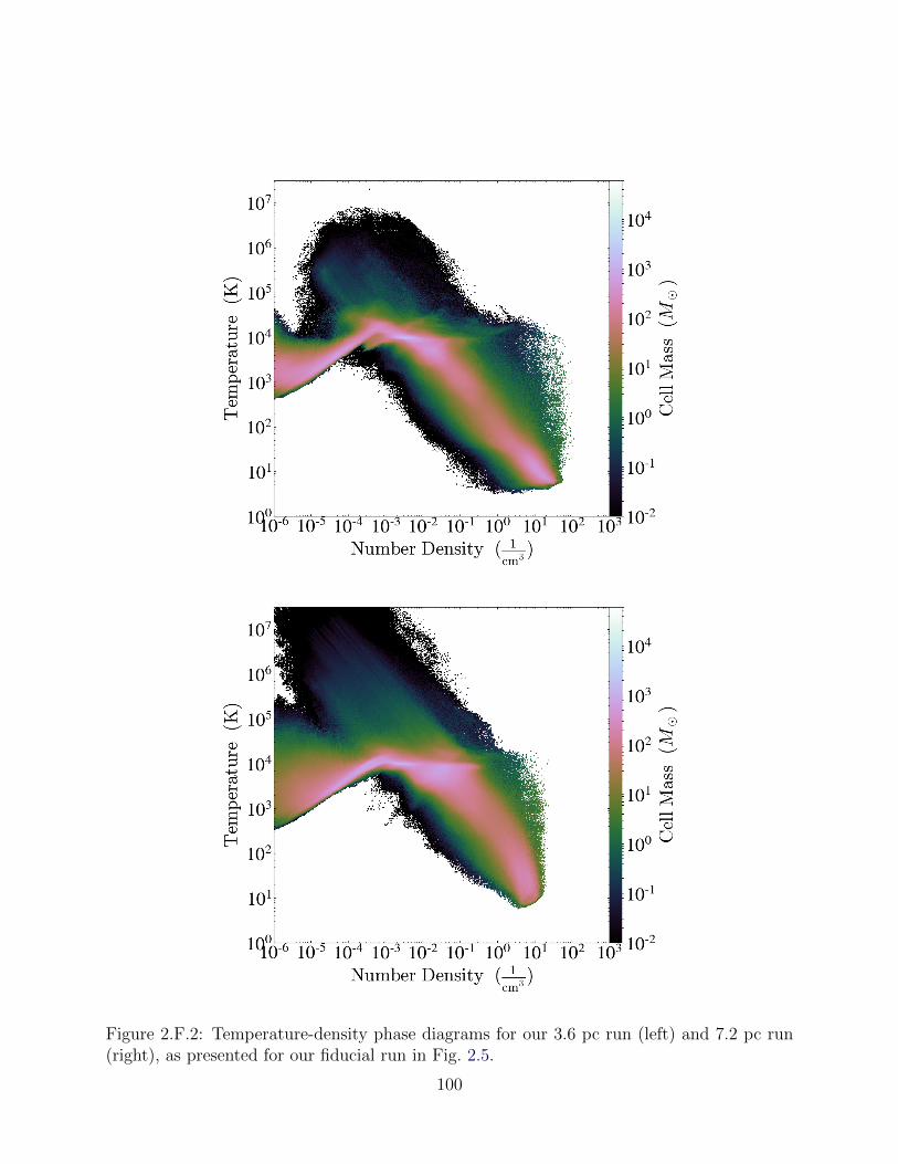
Figure 2.F.2: Temperature-density phase diagrams for our 3.6 pc run (left) and 7.2 pc run(right), as presented for our fiducial run in Fig. 2.5.
100
Finally, the metal retention fraction (right panel) between the fiducial and 3.6 pc runs
are quite similar, but is significantly higher for the lowest resolution simulation. It is likely,
however, that this is a result of the lower SFR in the 7.2 pc run and is not directly a
resolution effect. This also affects the fraction of metals ejected outside the virial radius,
with less metals being ejected in the lower resolution runs.
101

Chapter 3
Stellar Radiation is Critical for
Regulating Star Formation and
Driving Outflows in Low Mass Dwarf
Galaxies
3.1 Introduction
Historically, simulations of galaxy formation have suffered from the “overcooling” problem,
whereby the action of self-gravity and radiative cooling alone produces galaxies with far too
many stars. This problem has been addressed by employing various models of strong stellar
feedback physics which are capable of generating self-regulating star formation in galaxies
(see Somerville & Dave (2015) and Naab & Ostriker (2017) for recent reviews). Energy
injection from supernovae (SNe) has historically been used as the sole form of feedback.
This section contains text from an article published originally as Emerick et al. (2018a)
102

However, this is generally done heuristically as many simulations lack the ability to resolve
the Sedov phase of individual SNe. But even with this strong feedback, recent work has
argued for the need for pre-SN feedback, from stellar winds and/or stellar radiation (e.g.
Hu et al. 2016; Hopkins et al. 2018), though this is typically modeled simply as additional
energy injection around newly formed stars. The need for additional feedback is confirmed
by simulations that are capable of fully resolving individual SN (e.g. Peters et al. 2017; Smith
et al. 2018a,b; Hu 2018). However, modeling these processes in detail is challenging, and
their competing effects on galactic evolution are poorly constrained.
Radiation from massive stars dominates the total feedback energy output of a stellar
population (e.g. Abbott 1982; Leitherer et al. 1999; Agertz et al. 2013), surpassing the
energy ejection of supernova (∼ 1051 erg) by two orders of magnitude. If radiation couples
effectively to the interstellar medium (ISM), it can be a substantial source of additional
feedback. Simulations including stellar radiation feedback followed through radiative transfer
or radiation-hydrodynamics schemes have found it to be effective in regulating star formation
and driving galactic winds (e.g. Wise et al. 2012a; Kim et al. 2013a; Sales et al. 2014; O’Shea
et al. 2015; Rosdahl et al. 2015; Pawlik et al. 2015; Ocvirk et al. 2016; Peters et al. 2017). This
occurs in four ways: 1) heating of diffuse gas and preventing the formation of cold, dense star
formation regions, 2) destruction of cold, dense gas around recently formed stars, preventing
further star formation, 3) momentum input by direct absorption of UV radiation by gas and
(in some cases) dust through re-emission and scattering in the infrared, and 4) lowering the
typical ISM densities in which SNe occur and greatly increasing their effectiveness.
However, most works that employ stellar radiation feedback to account for these effects do
so using various forms of sub-grid, approximate models to avoid the substantial additional
cost of full radiative transfer. Many works use a Stromgren approximation whereby the
particles / cells within the Stromgren radius around a radiating star are heated and kept
103
ionized, with additional approximations made to account for overlapping ionized regions
(e.g. Hopkins et al. 2011; Hu et al. 2016, 2017). Other works employ some form of energy or
momentum injection localized to the region immediately around a star particle (e.g. Agertz
et al. 2013; Roskar et al. 2014; Ceverino et al. 2014; Forbes et al. 2016). Although some
of these approximate methods account for long-range effects of diffuse radiation (Hopkins
et al. 2012, 2018) most cases treat local radiation only, confined to energy or momentum
injection in a limited physical region around a star particle. This is done both because the
local destruction of dense clumps of gas around newly formed stars is commonly believed
to be the dominant impact of stellar radiation feedback and because it is computationally
less expensive to implement. The role of long-range stellar radiation, once ionizing photons
break out of star forming regions, is not well characterized. Indeed it remains to be seen if
modeling only the short-range effects of stellar radiation feedback is sufficient.
In this work we use a detailed model for stellar feedback presented in Emerick et al.
(2019) (hereafter Paper I) to study the role of radiation feedback in dwarf galaxy evolution.
For the first time in a galaxy-scale simulation, we resolve individual HII regions using an
adaptive ray tracing radiative transfer method to follow the ionizing radiation from particles
that represent individual stars. We focus on addressing two questions: 1) what role does
radiation feedback play in regulating star formation, and 2) are the long-range effects of
radiation feedback important, or is the local destruction of dense gas the dominant effect.
To investigate these questions, we compare three simulations of the evolution of an iso-
lated, low mass dwarf galaxy. Our fiducial model, containing full stellar radiation feedback,
is compared against a run without ionizing radiation feedback, and a run with ionizing feed-
back limited to the local region around a given star. We discuss our methods in Section 3.2
and present our results ion Section 3.3.
104

3.2 Methods and Initial Conditions
We refer the reader to Paper I for a more detailed description of our methods. We use
the adaptive mesh refinement hydrodynamics code Enzo (Bryan et al. 2014) to evolve an
idealized, isolated low mass dwarf galaxy. The galaxy is initialized as a smooth exponential
disk set in hydrostatic equilibrium with a static dark matter potential (Burkert 1995) with
Mgas = 2 × 10⁶ M�, Zgas = 4 × 10⁻⁴, radial and vertical gas scale heights of 250 pc
and 100 pc respectively, and Mvir = 2.48 × 10⁹ M�, on a grid with a maximum physical
resolution of 1.8 pc. We include no initial stellar population, but do include random driving
from supernovae as an initial source of feedback up until the onset of star formation.
We include a UV background, tabulated metal line cooling, and a 9 species non-equilibrium
chemistry solver using Grackle (Smith et al. 2017). Star formation occurs stochastically
in cold, dense regions (n > 200 cm−3, T < 200 K) by sampling a Salpeter (1955) IMF from
1 M� to 100 M� and depositing individual star particles over this mass range. We include
feedback from stellar winds, AGB winds, FUV and LW band radiation which drives pho-
toelectric heating and H2 dissociation respectively, HI and HeI ionizing radiation, and core
collapse and Type Ia SNe using thermal energy injection. FUV and LW band radiation are
both taken to be optically thin, with local (cell-by-cell) attenuation alone. Ionizing radia-
tion is followed using radiative transfer, as discussed below. Stellar lifetimes, surface gravity,
effective temperature, and radii are set by the initial stellar mass and metallicity through
interpolation over the PARSEC (Bressan et al. 2012) zero age main sequence values. These
properties are used to set the FUV, LW, and ionizing photon fluxes from each star through
interpolation on the OSTAR2002 (Lanz & Hubeny 2003) grid. We only model the radiation
from stars with masses above 8 M�.
Our fiducial simulation follows photoionizing radiation using the adaptive ray-tracing
105

radiative transfer method of Wise & Abel (2011). This method places and evolves 48 rays
on a HEALPix grid around each emitting source star for both HI and HeI ionizing radiation.
Rays are adaptively split as they propagate away from their source to increase the angular
resolution such that the solid angle of the ray remains smaller than 1/3 of the cell area.
Rays begin on HEALPix refinement level 2, with a maximum refinement level of 13. We
include radiation pressure on hydrogen, but do not investigate its importance in this work
(see Krumholz 2018, and references therein).
We additionally present a simulation run without any stellar ionizing radiation (“noRT”)
and a second simulation that includes ionizing radiation, but deletes all photons that travel
more than 20 pc from their source (“shortrad”). This second simulation tests the relative
importance of short-range vs. long-range effects of stellar ionizing radiation as a form of
feedback. Although this is still more accurate than an approximate method, this is meant to
function similarly to methods that include only the local effects of stellar radiation feedback.
Each of our three simulations is identical up until the formation of the first star particles.1
As shown in Paper I, the maximum densities reached in these simulations is below
103 cm−3. Our inability to resolve the high densities in star forming regions (∼ 105 cm−3)
means that we likely underestimate initial photon absorption and overestimate the initial
long-range effects of newly formed stars. However, in the Milky Way, newly formed O stars
have been observed to spend no more than 10 – 20% of their main sequence lifetimes em-
bedded in ultracompact HII regions within dense molecular clouds (Wood & Churchwell
1989). This short dispersal timescale agrees with high resolution simulations of massive star
1We note that the stars from the very first star formation event in each run (21 star particles with atotal mass of 114 M�) are the same. Of these, one particle emits ionizing radiation (M∗ > 8 M�). Thesampled stellar masses differ across runs after this point. Stochastic effects from differences in IMF samplingmay be important in the regime of low mass, low SFR dwarf galaxies. Multiple re-simulations of identicalinitial conditions may result in significant scatter in their final properties (Keller et al. 2018). We find ourmain conclusions are likely to be insensitive to these stochastic variations, as we find that the total radiationoutput across multiple re-samplings of a fixed star formation history is small after the IMF is fully sampled.
106
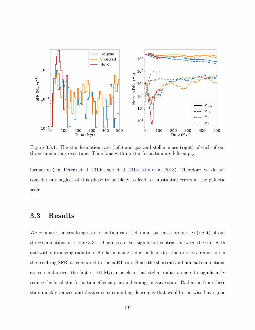
Figure 3.3.1: The star formation rate (left) and gas and stellar mass (right) of each of ourthree simulations over time. Time bins with no star formation are left empty.
formation (e.g. Peters et al. 2010; Dale et al. 2014; Kim et al. 2018). Therefore, we do not
consider our neglect of this phase to be likely to lead to substantial errors at the galactic
scale.
3.3 Results
We compare the resulting star formation rate (left) and gas mass properties (right) of our
three simulations in Figure 3.3.1. There is a clear, significant contrast between the runs with
and without ionizing radiation. Stellar ionizing radiation leads to a factor of ∼ 5 reduction in
the resulting SFR, as compared to the noRT run. Since the shortrad and fiducial simulations
are so similar over the first ∼ 100 Myr, it is clear that stellar radiation acts to significantly
reduce the local star formation efficiency around young, massive stars. Radiation from these
stars quickly ionizes and dissipates surrounding dense gas that would otherwise have gone
107
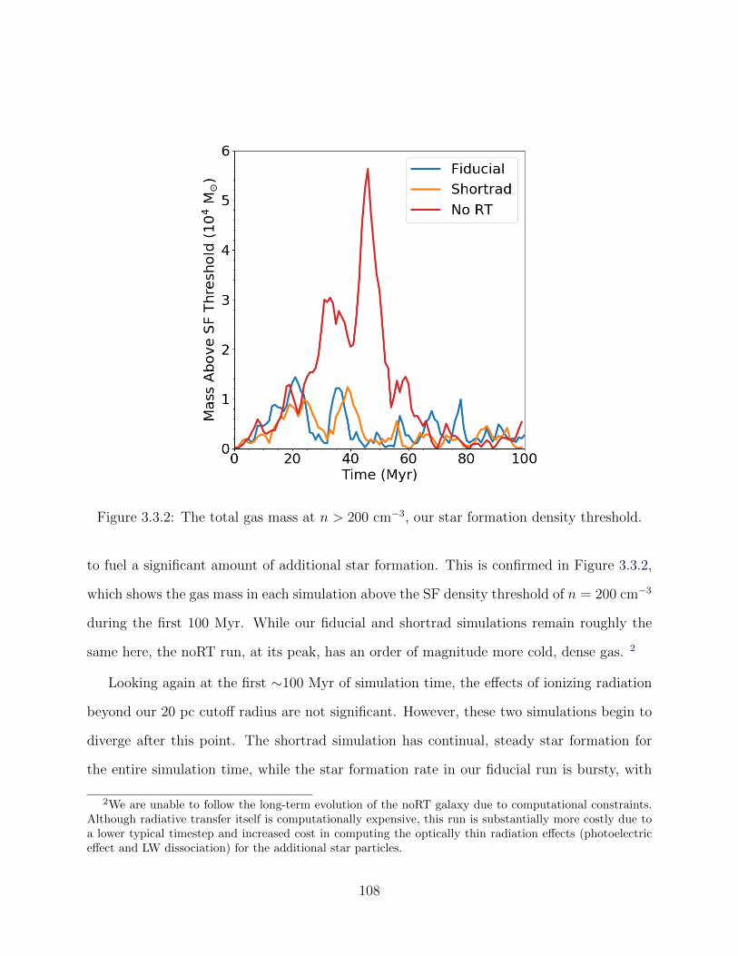
Figure 3.3.2: The total gas mass at n > 200 cm−3, our star formation density threshold.
to fuel a significant amount of additional star formation. This is confirmed in Figure 3.3.2,
which shows the gas mass in each simulation above the SF density threshold of n = 200 cm−3
during the first 100 Myr. While our fiducial and shortrad simulations remain roughly the
same here, the noRT run, at its peak, has an order of magnitude more cold, dense gas. 2
Looking again at the first ∼100 Myr of simulation time, the effects of ionizing radiation
beyond our 20 pc cutoff radius are not significant. However, these two simulations begin to
diverge after this point. The shortrad simulation has continual, steady star formation for
the entire simulation time, while the star formation rate in our fiducial run is bursty, with
2We are unable to follow the long-term evolution of the noRT galaxy due to computational constraints.Although radiative transfer itself is computationally expensive, this run is substantially more costly due toa lower typical timestep and increased cost in computing the optically thin radiation effects (photoelectriceffect and LW dissociation) for the additional star particles.
108

periods of active, low-level star formation interspersed with periods of no star formation.
The driver of these differences is clear in the right hand panel. Our fiducial run loses a factor
of ∼ 2 more total gas and HI mass (orange and blue lines) as compared to the shortrad
simulation. Clearly, galactic winds and outflows are much more effective in simulations with
a full accounting of stellar ionizing radiation feedback.
This can be confirmed by examining the metal retention fraction (the fraction of produced
metals retained within the disk of the galaxy) and mass outflow rates across simulations. As
shown in Figure 3.3.3, the mass outflow rate in the fiducial run peaks at an order of magnitude
higher at 0.25 Rvir than the shortrad simulation, declining only due to a comparative drop
off in star formation. The outflow in noRT is only a factor of a few lower than the fiducial
run, but it requires a five times higher supernova rate in this simulation to match the same
outflow seen with full stellar radiation feedback, so it implies a far lower mass loading factor.
Because of this difference in SFR, the differences across simulations are more significant for
our computed mass loading factor
η =Mout
< SFR >100Myr
. (3.1)
The brackets indicate time averaging over 100 Myr. While the fiducial run reaches a peak
η of a few hundred, shortrad is consistently an order of magnitude or more below this. The
noRT simulation is even lower.
The fiducial run is also the only one of the three with any significant outflow beyond
the virial radius. We conclude that radiation feedback allows SNe to be substantially more
effective in driving outflows.
109

Figure 3.3.3: Top Left: The fraction of metals contained within the ISM of each galaxy(blue) and the fraction ejected beyond the virial radius (orange). As in Figure 3.3.1, thefiducial run is given as solid lines, while the noRT and shortrad are dash-dotted and dashedrespectively. Top Right: The mass outflow rate for each run at 0.25 Rvir (solid) and Rvir
(dashed). Bottom: The mass loading factor η calculated as the outflow rate divided by theSFR averaged over 100 Myr. Inclusion of diffuse ionization makes an order of magnitudedifference in η in this case.
110
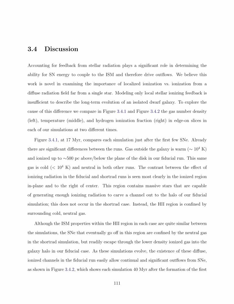
3.4 Discussion
Accounting for feedback from stellar radiation plays a significant role in determining the
ability for SN energy to couple to the ISM and therefore drive outflows. We believe this
work is novel in examining the importance of localized ionization vs. ionization from a
diffuse radiation field far from a single star. Modeling only local stellar ionizing feedback is
insufficient to describe the long-term evolution of an isolated dwarf galaxy. To explore the
cause of this difference we compare in Figure 3.4.1 and Figure 3.4.2 the gas number density
(left), temperature (middle), and hydrogen ionization fraction (right) in edge-on slices in
each of our simulations at two different times.
Figure 3.4.1, at 17 Myr, compares each simulation just after the first few SNe. Already
there are significant differences between the runs. Gas outside the galaxy is warm (∼ 104 K)
and ionized up to ∼500 pc above/below the plane of the disk in our fiducial run. This same
gas is cold (< 104 K) and neutral in both other runs. The contrast between the effect of
ionizing radiation in the fiducial and shortrad runs is seen most clearly in the ionized region
in-plane and to the right of center. This region contains massive stars that are capable
of generating enough ionizing radiation to carve a channel out to the halo of our fiducial
simulation; this does not occur in the shortrad case. Instead, the HII region is confined by
surrounding cold, neutral gas.
Although the ISM properties within the HII region in each case are quite similar between
the simulations, the SNe that eventually go off in this region are confined by the neutral gas
in the shortrad simulation, but readily escape through the lower density ionized gas into the
galaxy halo in our fiducial case. As these simulations evolve, the existence of these diffuse,
ionized channels in the fiducial run easily allow continual and significant outflows from SNe,
as shown in Figure 3.4.2, which shows each simulation 40 Myr after the formation of the first
111

Figure 3.4.1: Edge-on slices of each simulation showing gas number density (left), temper-ature (middle), and hydrogen ionization fraction (right) 17 Myr after the formation of thefirst star in each run. Each panel is 4 kpc x 4 kpc. See Emerick et al. (2018a) for a movieof this evolution.
112

Figure 3.4.2: Same as Figure 3.4.1, but at 40 Myr.
113
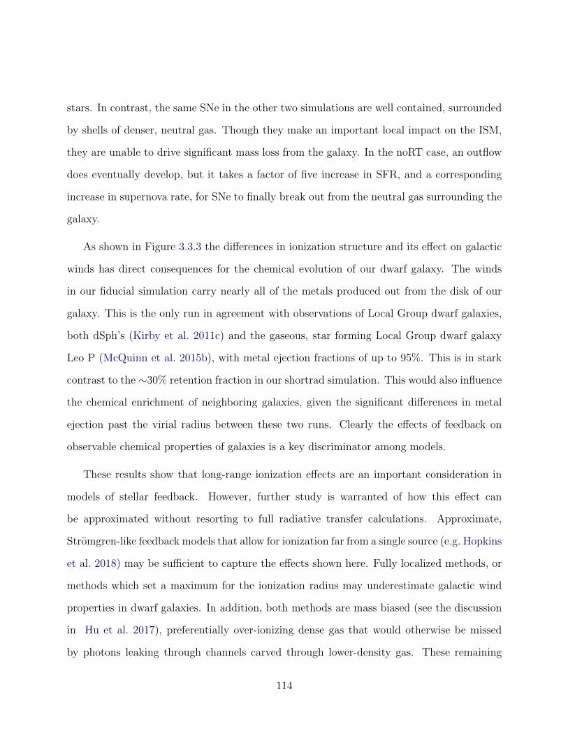
stars. In contrast, the same SNe in the other two simulations are well contained, surrounded
by shells of denser, neutral gas. Though they make an important local impact on the ISM,
they are unable to drive significant mass loss from the galaxy. In the noRT case, an outflow
does eventually develop, but it takes a factor of five increase in SFR, and a corresponding
increase in supernova rate, for SNe to finally break out from the neutral gas surrounding the
galaxy.
As shown in Figure 3.3.3 the differences in ionization structure and its effect on galactic
winds has direct consequences for the chemical evolution of our dwarf galaxy. The winds
in our fiducial simulation carry nearly all of the metals produced out from the disk of our
galaxy. This is the only run in agreement with observations of Local Group dwarf galaxies,
both dSph’s (Kirby et al. 2011c) and the gaseous, star forming Local Group dwarf galaxy
Leo P (McQuinn et al. 2015b), with metal ejection fractions of up to 95%. This is in stark
contrast to the ∼30% retention fraction in our shortrad simulation. This would also influence
the chemical enrichment of neighboring galaxies, given the significant differences in metal
ejection past the virial radius between these two runs. Clearly the effects of feedback on
observable chemical properties of galaxies is a key discriminator among models.
These results show that long-range ionization effects are an important consideration in
models of stellar feedback. However, further study is warranted of how this effect can
be approximated without resorting to full radiative transfer calculations. Approximate,
Stromgren-like feedback models that allow for ionization far from a single source (e.g. Hopkins
et al. 2018) may be sufficient to capture the effects shown here. Fully localized methods, or
methods which set a maximum for the ionization radius may underestimate galactic wind
properties in dwarf galaxies. In addition, both methods are mass biased (see the discussion
in Hu et al. 2017), preferentially over-ionizing dense gas that would otherwise be missed
by photons leaking through channels carved through lower-density gas. These remaining
114
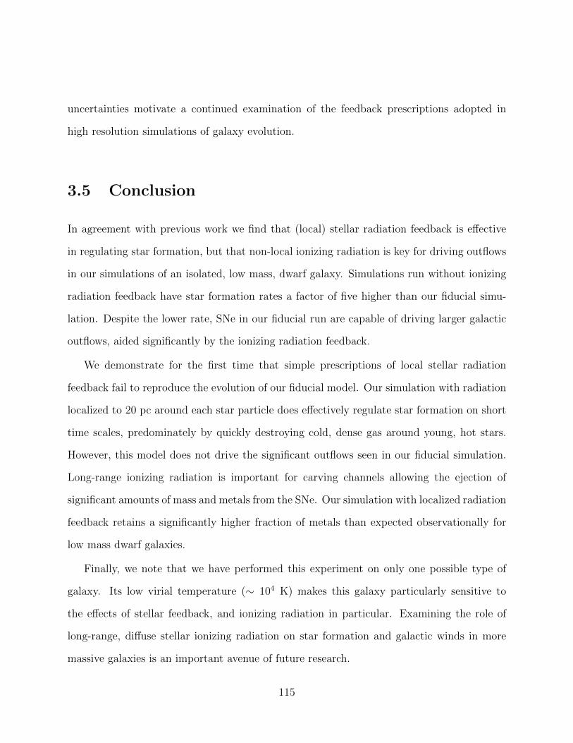
uncertainties motivate a continued examination of the feedback prescriptions adopted in
high resolution simulations of galaxy evolution.
3.5 Conclusion
In agreement with previous work we find that (local) stellar radiation feedback is effective
in regulating star formation, but that non-local ionizing radiation is key for driving outflows
in our simulations of an isolated, low mass, dwarf galaxy. Simulations run without ionizing
radiation feedback have star formation rates a factor of five higher than our fiducial simu-
lation. Despite the lower rate, SNe in our fiducial run are capable of driving larger galactic
outflows, aided significantly by the ionizing radiation feedback.
We demonstrate for the first time that simple prescriptions of local stellar radiation
feedback fail to reproduce the evolution of our fiducial model. Our simulation with radiation
localized to 20 pc around each star particle does effectively regulate star formation on short
time scales, predominately by quickly destroying cold, dense gas around young, hot stars.
However, this model does not drive the significant outflows seen in our fiducial simulation.
Long-range ionizing radiation is important for carving channels allowing the ejection of
significant amounts of mass and metals from the SNe. Our simulation with localized radiation
feedback retains a significantly higher fraction of metals than expected observationally for
low mass dwarf galaxies.
Finally, we note that we have performed this experiment on only one possible type of
galaxy. Its low virial temperature (∼ 104 K) makes this galaxy particularly sensitive to
the effects of stellar feedback, and ionizing radiation in particular. Examining the role of
long-range, diffuse stellar ionizing radiation on star formation and galactic winds in more
massive galaxies is an important avenue of future research.
115
Acknowledgments:
A.E. is funded by the NSF Graduate Research Fellowship DGE 16-44869. G.L.B. acknowl-
edges support from NSF AST-1312888, NASA NNX15AB20G, and NSF AST-1615955. M.-
M.M.L. was partly funded by NASA grant NNX14AP27G and NSF grant AST18-15461. We
gratefully recognize computational resources provided by NSF XSEDE through grant number
TGMCA99S024, the NASA High-End Computing Program through the NASA Advanced
Supercomputing Division at Ames Research Center, Columbia University, and the Flatiron
Institute. This work made significant use of many open source software packages, including
yt, Enzo, Grackle, Python, IPython, NumPy, SciPy, Matplotlib, HDF5, h5py,
Astropy, Cloudy and deepdish. These are products of collaborative effort by many
independent developers from numerous institutions around the world. Their commitment to
open science has helped make this work possible.
116
Chapter 4
Metal Mixing and Ejection in Dwarf
Galaxies is Dependent on
Nucleosynthetic Source
4.1 Introduction
Understanding galactic chemical evolution for all metal species across galaxy mass scales
remains one of the most challenging aspects of modeling galaxy evolution. One of the most
pressing difficulties is a lack of understanding in exactly how metals propagate from their
injection sites from stellar winds or supernovae (SNe) and mix through the phases of the
interstellar medium (ISM) into star-forming gas.
One-zone chemical evolution models assume homoegeneous mixing of metals from recent
star formation into gas available for future star formation (e.g. Lanfranchi et al. 2006; Kirby
et al. 2011a; Cote et al. 2017; Andrews et al. 2017). While this assumes that metal mixing
This section contains text from an article published originally as Emerick et al. (2018b)
117

in the ISM plays no role in delaying future enrichment in star formation, accounting for
this process is challenging. More complex models (e.g. Schonrich & Binney 2009; Pezzulli
& Fraternali 2016) employ multiple (usually radial) zones or follow multiple gas phases
to attempt to account for these effects. How to properly account for multi-phase mixing,
however, is still poorly understood. This is in large part because both these models and
large-scale cosmological simulations lack the necessary fidelity to capture the detailed, multi-
phase mixing process of metals in the ISM directly. Recent hydrodynamics simulations have
employed parametric models to account for unresolved sub-grid metal mixing (Pan et al.
2013; Sarmento et al. 2017, 2018), which plays an important role in determining the chemical
properties of galaxies (e.g. Shen et al. 2010; Pilkington et al. 2012; Few et al. 2012; Brook
et al. 2014; Feng & Krumholz 2014; Armillotta et al. 2018; Escala et al. 2018; Rennehan
et al. 2018) and the enrichment process and chemical signatures of the first stars (e.g. Jeon
et al. 2015; Ritter et al. 2015; Smith et al. 2015). Detailed hydrodynamics simulations
incorporating a multi-phase ISM and detailed stellar feedback are required to understand
the details of metal mixing and metal outflows in galaxies.
In addition, it remains to be seen to what degree, if at all, metals of different enrichment
origins (AGB winds, core collapse SNe, Type Ia SNe, neutron-star neutron-star mergers, etc.)
may couple differently to the ISM. When metals are tracked individually, as opposed to a
global metallicity field, their injection, mixing, and outflow properties are often treated uni-
formly. However, if metals do not behave uniformly in the ISM, if their mixing and ejection
behavior depends directly upon the energetics and physical environment of their injection,
then this assumption would need to be re-evaluated. Differences in metal distributions from
ejecta in AGB stars, as compared to SNe, has been explored recently in Krumholz & Ting
(2018), but has yet to be demonstrated in hydrodynamics simulations. Relaxing this as-
sumption has implications for both interpreting observations of stellar abundances in nearby
118

dwarf galaxies and in modeling galactic chemical evolution in both semi-analytic models and
lower resolution cosmological simulations (e.g. Cote et al. 2018).
The use of low mass dwarf galaxies, both observationally in the Local Group and in
theoretical models, has been critical in improving our understanding of galactic chemical
evolution. That dwarf galaxies efficiently pollute the circumgalactic medium and intergalac-
tic medium (IGM) with metals has been demonstrated for some time both theoretically (e.g.
Dekel & Silk 1986; Mac Low & Ferrara 1999; Fragile et al. 2004; Muratov et al. 2017; Corlies
et al. 2018), and with direct observational evidence from the metal retention fractions of
Local Group dwarf galaxies (e.g. Kirby et al. 2011b; Bordoloi et al. 2014; McQuinn et al.
2015b). If there are differences in metal coupling to the ISM, this could potentially impact
how metals are driven out of galaxies through galactic winds. This has implications for both
interpreting observations of stellar abundances in nearby dwarf galaxies and in modeling
galactic chemical evolution in both semi-analytic models and lower resolution cosmological
simulations. However, examining this process has only become possible recently as it re-
quires high resolution, galaxy-scale hydrodynamics simulations that can resolve ISM mixing
and self-consistently drive galactic winds through multi-channel stellar feedback.
It is becoming increasingly valuable to develop a concrete theoretical understanding of
galactic chemical evolution as a result of multiple, recent observational campaigns to probe
detailed stellar abundances in our Milky Way and the Local Group, such as SEGUE (Yanny
et al. 2009), RAVE (Kunder et al. 2017), APOGEE (Anders et al. 2014), and GALAH (Buder
et al. 2018). Stellar abundances are directly imprinted with the enrichment pattern of their
star-forming cloud, whose chemical properties are determined by the process of turbulent
metal mixing in the ISM. The degree to which we can associate ”chemically tagged” stars as
co-eval depends directly upon our understanding of metal enrichment and metal mixing in
the ISM. Furthermore, this understanding is critical for using these observations to further
119
deduce properties of a galaxy’s evolutionary history.
One key aspect of this work has been a significant effort to characterize the number of
independent dimensions accessible by the multi-dimensional chemical abundances observed
in these studies (e.g Freeman & Bland-Hawthorn 2002; Ting et al. 2012; Hogg et al. 2016;
Jofre et al. 2017; Price-Jones & Bovy 2018). Thus far, these studies have remained unin-
formed by hydrodynamics simulations and, conversely, these results cannot yet be used to
constrain simulations. Doing so requires the kinds of high resolution, galaxy-scale multi-
element chemodynamical simulations that have only become feasible in recent years. Recent
work has suggested that low-mass dwarf galaxies are perhaps the best regime to begin under-
standing these processes (e.g. Bland-Hawthorn et al. 2010b,a; Karlsson et al. 2012; Webster
et al. 2016). This is advantageous, as their small physical size and low star formation rates
makes conducting high resolution, hydrodynamics simulations of these systems computa-
tionally feasible.
In this paper we present the first detailed chemical evolution results from a set of high-
resolution hydrodynamics simulations of an isolated, low-mass, dwarf galaxy performed with
the adaptive mesh refinement code Enzo (Bryan et al. 2014). The simulation discussed here
was introduced in detail in Emerick et al. (2019) (hereafter Paper I). To address the out-
standing questions discussed above, these simulations follow star formation using individual
star particles, including stellar feedback from massive star and AGB-phase stellar winds,
photoelectric heating, Lyman Werner dissociation, ionizing radiation tracked through an
adaptive ray-tracing radiative transfer method, and core collapse and Type Ia SNe. This is
in addition to a detailed model for ISM physics using the Grackle library, as discussed
below. We show that metals are strongly ejected via galactic winds, but that the retention of
metals in the ISM and their mixing through phases varies significantly depending on the pro-
duction source of the given elemental species. We show how these elements are distributed
120

in the ISM and conclude with a discussion on the implications of these results.
The physical processes that drive galactic chemical evolution are complex, driven by the
details of stellar feedback, turbulence and diffusion in a multi-phase ISM, and variations
in stellar yields with nucleosynthetic source and stellar metallicity. Uncertainties in each
of these processes make reproducing and interpreting observations of gas and stellar abun-
dances challenging. These uncertainties, combined with the difficulty in simulating a fully
self-consistent galaxy in detail, motivates this current study. By focusing on a low mass
dwarf galaxy, with small size and low star formation rate, we can capture detailed feedback
and ISM physics at high resolution, while following individual stars. In this work we focus
on theoretical quantities, namely the probability density distributions (PDFs) of metals in
the ISM as a function of metal mass fraction, rather than the common observables of stellar
and gas abundance ratios, for two reasons. First, we would like to build our understanding of
galactic chemical evolution from a fundamental level. Second, there is only a limited sample
of gas-rich, star forming dwarf galaxies of this size that we can use for direct observational
comparison, and it is computationally infeasible to simulate galaxies of easily observable size
in as much detail as done here. This work will be the first of several attempting to bridge
this gap. With a more fundamental understanding of metal mixing and stellar enrichment
in galaxies, we can construct better one-zone chemical evolution models and physically mo-
tivated sub-grid physics models for lower resolution simulations of more massive galaxies.
We summarize our methods and physics models in Section 4.2. We begin our analysis by
presenting the only direct observable comparison we can make at this galaxy mass, discussing
the metal retention fractions of our galaxy in Section 4.3.1. In Section 4.3.2.1 we focus on
how each of our 15 individual metal species are distributed and evolve within each phase of
the ISM. We discuss our results in Section 4.4, and conclude in Section 4.5.
121
4.2 Methods
We refer the reader to Paper I for a detailed description of our numerical methods and
feedback models. We briefly summarize the relevant details here.
Hydrodynamics We use the adaptive mesh refinement astrophysical hydrodynamics and
N-body code Enzo1 (Bryan et al. 2014). Hydrodynamics are solved using a direct-Eulerian
piecewise parabolic method and a two-shock approximate Riemann solver with progressive
fallback to more diffusive solvers. We include gas self-gravity and evolve collisionless star
particles using a particle mesh N-body solver. We use a 1283 base grid with outflow boundary
conditions measuring 2.16 Rvir on a side, where Rvir = 27.4 kpc, and 9 levels of refinement,
for a maximum spatial resolution of 1.8 pc. Refinement occurs when either: 1) a cell contains
more than 50 M� of gas or 2) a cell’s local Jeans length becomes resolved by less than eight
cells. Also, if the cell is within four zones of a star particle with active feedback, it is refined
to the maximum resolution. At the maximum resolution, we use a pressure floor to prevent
artificial fragmentation when the Jeans length is unresolved.
Chemistry, Heating, and Cooling Physics We use the the astrophysical chemistry and
cooling package Grackle (Smith et al. 2017) to evolve a nine species non-equilibrium pri-
mordial chemistry model (H, H+, He, He+, HeP++, H−, H2, H+2 , and e−), follow approximate
metal line cooling using a Cloudy look-up table, and apply heating from a metagalactic
UV background (Haardt & Madau 2012). We account for approximate self-shielding of H i
against the UV background following Rahmati et al. (2013). We assume He i self-shields
in the same fashion as H i, and ignore He ii heating from the UVB entirely. Approximate
H2 self-shielding from background Lyman-Werner (LW) radiation is accounted for using the
1http://enzo-project.org/
122
Sobolov-like method from Wolcott-Green et al. (2011). Finally, we use the updated metal
line cooling tables which self-consistently account for the decrease in metal line cooling rates
due to lower ionization fractions in self-shielding gas, as compared to metal cooling tables
computed under the optically thin assumption.
Star Formation Stars are followed as individual star particles from 1 M� to 100 M�. Stars
are able to form in dense gas with: 1) n > 200 cm−3, 2) T < 200 K, and 3) ∇ · v < 0. Given
the short time-steps (dt ∼ 500 yr) and high resolution (1.8 pc) in these simulations, the local
star formation rate in any single zone is very small (� 1 M� dt−1). We therefore form stars
stochastically, depending upon the local gas mass, free-fall time, and star formation efficiency,
εf , taken to be 2% (Krumholz & McKee 2005). Stellar masses are randomly sampled from
an assumed Salpeter (1955) IMF with metallicities and metal fractions set by the local gas
environment. We use the zero age main sequence properties of stars from the PARSEC
stellar evolution tables (Bressan et al. 2012; Tang et al. 2014) to determine individual stellar
lifetimes and properties which are used to set their LW band, far ultraviolet (FUV) band,
and ionizing radiation luminosities (see below).
Stellar Feedback and Stellar Yields We track the feedback and yields of 15 metal
species for each star individually. Stars between 8 M� < M∗ < 25M� explode as core
collapse SNe at the end of their life, injecting their mass and 1051 erg of thermal energy into
a spherical region with radius of 5.4 pc, or 3 times the maximum resolution. Stars above
this mass are assumed to direct collapse with no mass or energy injection. For all stars
above 8 M� we follow their stellar winds assuming continuous mass loss over their lifetimes,
their LW and FUV radiation as optically thin radiation which contributes to H2 dissociation
and photoelectric heating respectively, and their H i and He i ionizing radiation using an
adaptive ray-tracing radiative transfer method (Wise & Abel 2011). We interpolate over
123

the OSTAR2002 (Lanz & Hubeny 2003) grid to set the luminosities of each of these stars.
Low mass stars, M∗ < 8 M�, do not produce feedback during their main sequence lifetimes,
but end their lives injecting a short-lived, low velocity (10 km s−1) AGB wind (Goldman
et al. 2017). Stars with 3 < M∗ < 8 are tracked after their death as possible Type Ia SN
progenitors, using a delay time distribution model to assign when (if at all) they will explode
as a Type Ia, injecting 1051 erg of thermal energy with yields. Stellar yields are computed
using the NuGrid stellar yield database (Ritter et al. 2018b) for all stars with M∗ < 25 M�,
Slemer et. al. in prep for the stellar winds of stars with M∗ > 25 M�, and Thielemann et al.
(1986) for Type Ia SNe.
Initial Conditions Our dwarf galaxy is initialized to approximate, but not reproduce,
the z = 0 properties of an ultrafaint dwarf galaxy (UFD) as informed by the observed
properties of Leo P (see Giovanelli et al. 2013; McQuinn et al. 2015a,b). We initialize a
Mgas = 1.8×10⁶ M� disk as an exponential profile with a metal mass fraction of Z = 4.3×10⁻⁴
centered on a static Burkert (1995) dark matter potential with Mvir = 2.5 × 10⁹ M�. The
gas scale radius and scale height are set to 250 pc and 100 pc respectively, with a maximum
radial extent of 600 pc. Both the gas temperatures and velocities are set iteratively to enforce
initial hydrostatic equilibrium. The galaxy contains no initial background stellar population,
limiting the number of Typa Ia SNe in our model. We include initial SN driving to limit the
transient burst of star formation from the initial cooling and collapse of the galaxy. These
SNe are randomly distributed with the same radial and vertical scale heights as the gas disk
at a rate of 0.4 Myr−1; this corresponds to the current SFR of Leo P, ∼ 4 × 10⁻⁴ M� yr−1
(McQuinn et al. 2015a), assuming 1 SNe per 100 M� of star formation. The metal yields
from these SNe are set to the mean ISM abundances, and thus do not contribute to the
chemical evolution of the galaxy. Although the total metallicity field is initially non-zero, we
124
only track the self-consistently produced metal enrichment for each individual metal species
in our simulation, setting their initial abundances to zero. Our analysis is based on the
evolution of this galaxy during the first 500 Myr after the formation of the first star particle.
4.3 Results
For context, in Paper I we focused on the global properties of the evolution of this dwarf
galaxy, including an analysis of the galaxy’s gas mass and star formation evolution, the ISM
properties in terms of mass fractions, volume fractions, and phase diagrams, the interstellar
radiation field in each tracked radiation band, the gas outflow rates and galactic wind veloc-
ities, and the retention / ejection of metals from the galaxy. This galaxy has an average star
formation rate of 1.2 ×10⁻⁴ M� yr−1 and is consistent with observed low mass dwarfs galax-
ies in the Kenicutt-Schmidt relation. The galaxy exhibits strong, feedback-driven outflows
(Emerick et al. 2018b) that eject a significant amount of gas and metals from the galaxy.
The mass loading factor at 0.25 Rvir was found to be η ∼ 50, where η is defined as the mass
outflow rate in through a 0.1 Rvir annulus centered at 0.25 Rvir divided by the 100 Myr
averaged SFR. These winds eject 96% of the metals produced in the galaxy, with 50% of all
metals leaving the virial radius by the end of the simulation time.
In this work we focus in detail on how each of the 15 individual metal species evolve in this
galaxy. We address differences between the ejection fractions of each metal in Section 4.3.1
and analyze for the first time the mass-fraction PDFs of the metals retained by the ISM in
Section 4.3.2.
125

Figure 4.3.1: Top: The mass fraction of each metal species in the full simulation box con-tained in the halo, gas in the galaxy disk, and stars. Bottom: The mass fraction of specieswithin the disk alone in each phase of the ISM (bottom). The leftmost bar in each plotshows the sum of all metals.
126
4.3.1 Preferential Ejection of Metals from the ISM
The top panel of Figure 4.3.1 gives the mass fraction of each element at the end of the simula-
tion (500 Myr) in each of four reservoirs: locked in stars (yellow), in the ISM (blue), outside
the galaxy but within the virial radius (purple), and outside the virial radius (salmon), in-
cluding gas that has left the domain. We subdivide the ISM by phase in the bottom panel,
giving the mass fractions of each element in the cold neutral medium (CNM, fH2 < 0.5,
T< 100 K), warm neutral medium (WNM, 102 K ≤ T < 104 K), warm ionized medium
(WIM, 104 K ≤ T < 105.5 K), the hot ionized medium (HIM T≥ 105.5 K), and locked in
stars (yellow).2 We only consider metals produced self-consistently through our star forma-
tion and stellar feedback methods; the initial mass of each metal species is zero.
We find two major results. First, only a small fraction of produced metals are retained
within the dwarf galaxy, in agreement with observations of nearby dwarf galaxies (see Kirby
et al. 2011b; McQuinn et al. 2015b); however, the retention factor varies among elements.
The top panel shows a qualitative disagreement between the retention fractions of N and
Ba (about 20% for each) as compared to the rest of the metals (∼ 4 – 5%). This suggests
that individual metals do not share the same dynamical evolution. Thus, metal enrichment
in galaxies is a phenomenon that cannot be fully captured using a single, global metallicity
field. In this particular case, assuming that all metals behave the same would underestimate
the N and Ba enrichment by a factor of up to five, at least for low mass dwarf galaxies.
Second, nearly all of the metals retained in the disk reside within neutral gas, mostly
in the CNM; only a few percent reside in the hot phases. The exact fraction varies with
each species, most notably for carbon; these fluctuations are at most ∼ 10%. This is not
surprising, as the cold phases represent the majority of the mass in the ISM, but, as shown
2The fH2restriction on the CNM is not relevant in our simulations, as there are no cells with fH2
> 0.5.fH2
remains below about 0.35 for all cells (see Paper I).
127

Figure 4.3.2: The fraction of total mass in each metal species produced by each of the fourpossible nucleosynthetic channels in our model. These channels differ in both when metalsare ejected, as determined by stellar evolution, and the phase of the ISM into which they areejected. We note that the minimal contribution from Type Ia SNe for the iron-peak elementsis because no older stellar population was initialized, so only 16 of them have exploded bythe end of our 500 Myr simulation.
in Section 4.3.2.3, even though the cold phases harbor most of the metals, the hot phases
have significantly higher metal mass fractions.
The only physics that separates the dynamical evolution of these elements in our simu-
lations is the individual sources of enrichment: AGB winds (stars less than 8 M�), stellar
winds (stars above 8 M�), core collapse SNe, and Type Ia SNe. These channels differ in: 1)
how long after a given star formation event they occur, 2), by consequence, the typical ISM
properties in which they occur, and 3) how much energy is associated with each event, which
determines ejecta temperature and velocity. To understand where each of the elements in
Figure 4.3.1 originated, we show the mass fraction of metals produced through each channel
in Figure 4.3.2. Core collapse SNe are responsible for over 90% of the total metal enrichment
in our galaxy, but this is clearly not true for all elements. In particular, a majority of N
128
(74%) and Ba (65%) are ejected by AGB winds; both are retained at a higher rate than the
rest of the metals. That this behavior exists for N and Ba in our simulations is dependent
upon the metallicity of our galaxy and choice of stellar yield tables, but we can generalize this
result to say that, for any assumed set of yields, low mass galaxies should more easily retain
any elements synthesized predominately in AGB winds, as compared to elements synthesized
through SNe.3 We discuss how this result may extend towards other metal yields that are
not well sampled on our relatively short (500 Myr) simulation timescales in Section 4.4.3.
AGB winds have low energy and velocities (10 km s−1) as compared to the energy and
typical expansion velocities of SNe (∼1000 km s−1). In addition, their longer timescales
relative to massive stars means that AGB stars are typically removed from their birth regions
and randomly distributed through the galactic disk. The changes in typical ISM density and
height of these events contributes to these variations. We show histograms of the average
number density within 20 pc of any given enrichment source (top) and height above/below the
disk (bottom) within 1 Myr of each event (as limited by our output cadence) in Figure 4.3.3.
As shown, SNe peak at very low densities, indicating that most explode in superbubbles,
regions carved out by previous SNe. AGB stars predominately release their metals close to
the average ISM density. The scale height distributions for both events show no significant
differences. We do not expect these differences to be the dominant effect in driving the
differential evolution of elements ejected by AGB winds vs. SNe, compared to the energetics,
but can certainly play a significant role in determining the mixing behavior of individual
enrichment events. The changes to mixing behavior as a function of ISM properties will be
investigated in more detail in a future work.
3One might expect that much of the N and Ba that is ejected by galactic winds is comprised mostly ofthe ∼30% of each species produced through the stellar winds of more massive stars and SNe. However, thiscannot be proven as we lack Lagrangian information about individual gas elements.
129

Figure 4.3.3: The volume-averaged gas number densities within 20 pc of a given event (top)and vertical position above/below the disk (bottom) within 1 Myr before the event.
130

4.3.2 Mixing and Distribution of Metals in the ISM
We characterize the metal distributions (in Sections 4.3.2.1 and 4.3.2.2) and evolution (in
Section 4.3.2.3) in our galaxy to build towards a a complete model for how metals mix and
evolve in the complex, multi-phase ISM of real galaxies.
4.3.2.1 A Functional Form for Metal PDFs
The log-normal distribution is found often in nature, generally describing multiplicative
processes with non-negative values that grow with time. In astrophysics, for example, the
log-normal distribution can be used to describe the time evolution of the star formation rate
density (see Gladders et al. 2013; Abramson et al. 2016; Diemer et al. 2017). In addition,
as expected from analytic theory (Vazquez-Semadeni 1994), isothermal turbulence gives rise
to log-normal density probability distribution functions (PDFs; Padoan et al. 1997; Passot
& Vazquez-Semadeni 1998; Ostriker et al. 1999; Padoan & Nordlund 2002; Krumholz &
McKee 2005; Federrath et al. 2008). Although these PDFs are only log-normal in simulations
containing a more realistic, multi-phase ISM (Scalo et al. 1998) if the disk is very stable
(Wada & Norman 2007), individual phases within the ISM do exhibit some log-normality
(Tasker & Tan 2009; Tasker 2011; Joung et al. 2009; Price et al. 2011; Hopkins et al. 2012). It
has been shown that the 3D density PDF and the column density PDF, in both simulations
and observations, have a characteristic shape (Vazquez-Semadeni 1994; Burkhart et al. 2009;
Federrath & Klessen 2013; Collins et al. 2012; Myers 2015; Burkhart et al. 2017; Chen et al.
2018). This includes a log-normal component, generated by multiplicative processes—in
this case shocks and the turbulent cascade in the ISM—and a power-law component at high
densities arising from the additive combination of individual, self-gravitating cloud structures
.
131

The physics that drives the density PDF is directly related to the process of metal mixing
and diffusion. However, there is no a priori reason why gas density and metallicity PDFs
should have similar functional forms. We demonstrate here for the first time that the mass
fraction PDFs for each metal species in our simulation can indeed be well fit using a piecewise
log-normal + power-law PDF. We use a simple conceptual model in Section 4.4.1 to motivate
the emergence of this distribution.
We follow Collins et al. (2012), Burkhart et al. (2017), and Chen et al. (2018) in con-
structing our piecewise PDF. We define the distribution of metals in the ISM as a function
of the fraction of mass contained at a given metallicity, Z, or metal mass fraction, Zi, where
i denotes an individual element. This PDF is given as
p(Z) =
N
σZ√
2πexp
[− (ln(Z)−µ)2
2σ2
], Z < Zt
NpoZ−α, Z > Zt
where N is a normalization constant, po ensures continuity between the two components, µ
and σ are the log-mean and width of the log-normal component, α is the power-law slope, and
Zt is the metal fraction at the transition between the log-normal and power-law components.
When fitting this PDF, we only enforce continuity and∫∞
0p(Z)dZ = 1, leaving α, µ, σ, and
Zt as free parameters. These conditions set N and po to
N =1
2
[1 + erf
(ln (Zt)− µ
σ√
2
)]+
poα− 1
Z−α+1t (4.1)
and
po =1
σZt
√2π
exp
[−(ln(Zt)− µ)2
2σ2+ αln(Zt)
](4.2)
.
132
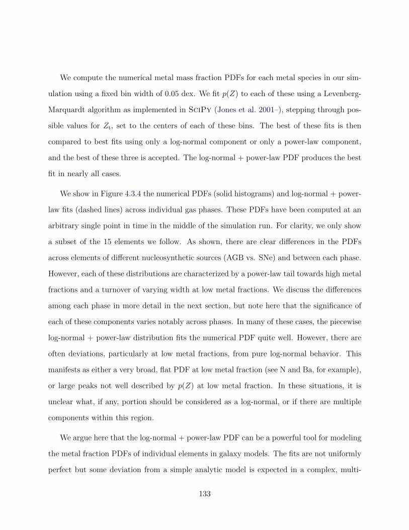
We compute the numerical metal mass fraction PDFs for each metal species in our sim-
ulation using a fixed bin width of 0.05 dex. We fit p(Z) to each of these using a Levenberg-
Marquardt algorithm as implemented in SciPy (Jones et al. 2001–), stepping through pos-
sible values for Zt, set to the centers of each of these bins. The best of these fits is then
compared to best fits using only a log-normal component or only a power-law component,
and the best of these three is accepted. The log-normal + power-law PDF produces the best
fit in nearly all cases.
We show in Figure 4.3.4 the numerical PDFs (solid histograms) and log-normal + power-
law fits (dashed lines) across individual gas phases. These PDFs have been computed at an
arbitrary single point in time in the middle of the simulation run. For clarity, we only show
a subset of the 15 elements we follow. As shown, there are clear differences in the PDFs
across elements of different nucleosynthetic sources (AGB vs. SNe) and between each phase.
However, each of these distributions are characterized by a power-law tail towards high metal
fractions and a turnover of varying width at low metal fractions. We discuss the differences
among each phase in more detail in the next section, but note here that the significance of
each of these components varies notably across phases. In many of these cases, the piecewise
log-normal + power-law distribution fits the numerical PDF quite well. However, there are
often deviations, particularly at low metal fractions, from pure log-normal behavior. This
manifests as either a very broad, flat PDF at low metal fraction (see N and Ba, for example),
or large peaks not well described by p(Z) at low metal fraction. In these situations, it is
unclear what, if any, portion should be considered as a log-normal, or if there are multiple
components within this region.
We argue here that the log-normal + power-law PDF can be a powerful tool for modeling
the metal fraction PDFs of individual elements in galaxy models. The fits are not uniformly
perfect but some deviation from a simple analytic model is expected in a complex, multi-
133

phase ISM. In addition, some of this deviation, particularly in the WNM and WIM, could
be caused by grouping together qualitatively distinct gas in a single phase; this would tend
to broaden the distributions. Most importantly, however, the PDFs of the CNM, are indeed
well fit by the adopted p(Z). As this is the source of star-forming gas in the ISM, the log-
normal + power-law PDF appears useful to account for intrinsic scatter in stellar abundances
in galaxy evolution models.
4.3.2.2 PDF Variation Across Gas Phase
The various phases represented in Figure 4.3.4 involve variations in density and temperature
of more than six orders of magnitude. The evolution of each phase is qualitatively different,
and the metal mixing behavior of each should vary. Mixing timescales over a given length
scale should be related to the local sound speed; hot gas, with higher sound speeds, should
mix more rapidly than the dense, disconnected clumps of cold gas in the ISM. In addition,
one would expect a metallicity gradient with gas temperature as enrichment occurs first in
the hot phases, cooling and enriching denser gas over time. We examine the PDF variations
among elements in each phase, as shown in Figure 4.3.4, in more detail here.
Unsurprisingly the diffuse HIM is the most metal rich phase, as it is comprised pre-
dominately of metal enriched SN ejecta. Clearly this leads to long power-law tails towards
high metal fractions for each species, with a very narrow, poorly defined peak at low metal
fractions. Generally, in colder gas the metal PDFs become less enriched with broader, low-
metal-fraction components and steeper, power-law tails. Although the extended power-law
tail of the HIM leads to a large range of metal fractions, the HIM represents very little mass,
and this tail represents recent, un-mixed enrichment. The comparatively narrow width in
the log-normal regimes of the CNM is perhaps surprising. Although this gas is at lower
metal fraction than the WNM and WIM, it would appear that it is more well mixed. This
134

Figure 4.3.4: The numerical PDFs (solid histograms) and the associated log-normal + power-law fits (dashed lines) for a subset of the elements tracked in our simulation in each of thefour gas phases defined in Section 4.3.1: CNM (dark blue), WNM (light blue), WIM (lightorange), HIM (red), and all the gas in the ISM (black). For clarity, each distribution isnormalized to the mode of the full-disk PDF (black) and is centered on the median value ofthe full-disk PDF. We note the vertical axis normalization is such that integrating over theshown PDF gives the mass fraction of that phase in the disk. Since the CNM dominates themass fraction of our galaxy, the black curve is often obscured at low metal fractions.
135

runs counter to the idea that mixing times should be long in colder gas, unless (as we argue)
mixing first proceeds rapidly in the hot phases before mixing in with cold, disconnected
structures across the galaxy.
Although these trends across phases hold for all elements, there are qualitative differences
between elements, particularly between those ejected predominantly by AGB winds (e.g. Ba
and N) and those ejected by SNe (e.g. O and Mg). In all phases, except the HIM, the
AGB-wind elements have broader distributions that are less well described by our adopted
p(Z) than the metals dominated by SN enrichment. The power-law component of N and Ba
is generally shallower than all other metals across each phase (except the HIM), particularly
in the CNM. Ba and N do not show significant differences among the rest of the metals in
the HIM, though this is likely because the Ba and N present in this phase is dominated by
the Ba and N included in SNe yields. Again these differences between yield sources could
be driven both by differences in their enrichment timescales and therefore differences in the
typical ISM environment each event encounters, and the differences in energetics between
AGB winds and SNe. AGB wind elements enrich the WNM and WIM directly, rather than
the HIM. This leads to longer mixing timescales and broader PDFs for these elements.
4.3.2.3 The Time Evolution of Metal PDFs
We focus on the time evolution of the full numerical PDFs in this section. Our results here
do not depend upon the choice of functional form for p(Z). Figure 4.3.5 shows the evolution
of four different statistics for the O (top) and Ba (bottom) PDFs. These two elements
are treated as representative elements for SN and AGB wind production respectively. The
difference between the mean and median masses of the PDF (second column) is a measure
of the skew of the PDF. Positive values indicate that metals are preferentially sequestered
in metal-rich gas, and are less well mixed throughout the given phase. The skew is always
136
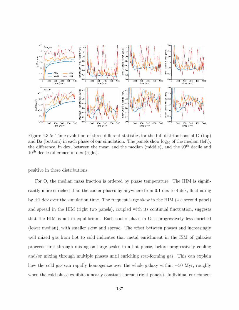
Figure 4.3.5: Time evolution of three different statistics for the full distributions of O (top)and Ba (bottom) in each phase of our simulation. The panels show log10 of the median (left),the difference, in dex, between the mean and the median (middle), and the 90th decile and10th decile difference in dex (right).
positive in these distributions.
For O, the median mass fraction is ordered by phase temperature. The HIM is signifi-
cantly more enriched than the cooler phases by anywhere from 0.1 dex to 4 dex, fluctuating
by ±1 dex over the simulation time. The frequent large skew in the HIM (see second panel)
and spread in the HIM (right two panels), coupled with its continual fluctuation, suggests
that the HIM is not in equilibrium. Each cooler phase in O is progressively less enriched
(lower median), with smaller skew and spread. The offset between phases and increasingly
well mixed gas from hot to cold indicates that metal enrichment in the ISM of galaxies
proceeds first through mixing on large scales in a hot phase, before progressively cooling
and/or mixing through multiple phases until enriching star-forming gas. This can explain
how the cold gas can rapidly homogenize over the whole galaxy within ∼50 Myr, roughly
when the cold phase exhibits a nearly constant spread (right panels). Individual enrichment
137

events have significantly higher metallicities than the ambient ISM in any phase, and drive
an increase in the difference between the mean and median of the PDF. These can be seen
as the obvious spikes in the HIM and WIM. For O, the lack of these spikes in the two cold
phases suggests again that enrichment does not occur directly in these phases, but proceeds
more gradually through the warmer phases first.
Although these trends are generally true for Ba, its evolution is much more complicated.
Unlike O, the spread and skew in Ba for the CNM, WNM, and WIM increase during the
evolution, reaching differences in 90th and 10th percentiles of nearly 2 dex in the CNM and
over 2 dex in the WNM and WIM. The HIM is seemingly unaffected by this trend, and
simply fluctuates throughout the simulation. Given their lower energies, AGB winds more
directly enrich the WNM and WIM, not the HIM as in SNe. The consequence of this is clear
in Figure 4.3.4 by the wider PDFs and longer power-law tails in Ba in these phases. These
tails represent the most recently enriched gas, which is clearly much more locally confined
than O.
The positive skew in all of the PDFs presented here implies that most of the mass of the
galaxy has a metal fraction below what one would normally adopt as the average metallicity
(i.e. the ratio between the total mass of metals and the total mass). Assuming star-forming
gas follows the same properties as the cold gas, this distinction is small (∼ 0.2 dex), though
significant, for elements released during SNe explosions, but can be very significant, up to ∼
0.8 dex, for elements released in AGB winds. Chemical evolution models, especially one-zone
models, follow the mean metal fraction, rather than the median. Our results indicate that
such models are biased to overestimate gas and stellar elemental abundances.
To summarize, Figure 4.3.5 demonstrates: 1) there are qualitative differences in how SN-
injected elements (e.g. O, Mg) and AGB-wind-injected elements (e.g. N, Ba) are distributed
through the ISM, with the latter having a broader range of variation and being less well
138
mixed in all phases except the HIM; 2) hotter phases are more metal enriched, both because
the cooler phases make up most of the initially unenriched mass of the ISM and because the
hotter phases are more directly populated by recent enrichment events; 3) the cooler, denser
phases, particularly for SN injected elements, are more well mixed than the hot phases of the
ISM; 4) the PDFs of metal mass fraction are best fit by a log-normal + power law function;
and therefore 5) the median metallicity available for star formation lies below the mean
galactic value. In the case of SN injected elements, enrichment proceeds quickly through the
HIM over the entire galaxy. For AGB injected elements, enrichment proceeds through the
WIM and WNM, leading to longer mixing timescales and larger metal fraction variations in
the ISM.
4.4 Discussion
We begin with a simple toy model that motivates the power-law tail at high metal fractions
of the metal fraction PDFs and a subsequent turnover at low metal fractions in Section 4.4.1.
This work is placed in context with previous papers focusing on metal mixing in the ISM in
Section 4.4.2. We discuss the relevance of additional AGB yields not directly followed in this
study in Section 4.4.3. Finally, in Section 4.4.4 we discuss how these results relate to stellar
abundances, make generalizations to more massive galaxies in Section 4.4.5, and discuss
possible impacts of these results on chemical enrichment from more exotic nucleosynthetic
sources in Section 4.4.6.
4.4.1 Physical Interpretation of the PDF
Take the simple case of an initially primordial, uniform, isothermal medium of mass Mo with
initial metallicity Zo, containing a single, un-mixed enrichment event of mass Mej whose size
139

is small compared to the system and mass Mej/Mo � 1. Thus the background medium
represents a virtually inexhaustible (but finite) source of un-enriched gas. In this case,
p(t, Z) initially takes the form of a double-delta function
p(to, Z) = δ(Zo) +Mej
Mo
δ(Z − Zej). (4.3)
If the enriched material mixes continually with the un-enriched gas at a constant rate,
after some time τmix this gas will have mixed with an equal amount of primordial gas. At
this time, p(τmix, Z) = δ(Zo) + (2Mej/Mo)δ(Z − (1/2)Zej). Then, p(2τmix, Z) = δ(Zo) +
(4Mej/Mo)δ(Z − (1/4)Zej), and so on for other multiples of τmix. This represents an inverse
relationship between the mass of enriched gas and the metallicity of the enriched gas. The
superposition of the distributions of a single event evolving in time will appear as a power-law
distribution with slope α = 1.
Thus, if the gas is continually enriched by identical, well-separated enrichment events of
mass Mej and metallicity Zej, the instantaneous distribution p(t, Z) of these many events will
be δ(Zo) plus a power law in Z with slope α = 1, truncated at some minimim Z (related to
the time since enrichment began) and some maximum, Zej. The slope of the power-law, then,
is determined by the rate of injection versus mixing with the ambient medium. A power-law
index α < 1 can occur when injection occurs more rapidly than the newly enriched gas
can mix with the ambient medium. Steeper power-laws, α > 1, develop when mixing occurs
more rapidly than injection. If the ambient, primordial gas were truly infinite, the power-law
would never completely encompass the delta function at Z = Zo.
In reality, however, Mo is not an inexhaustible reservoir of primordial gas. Eventually
the entire ambient medium will become enriched to some Z > Zo, and p(Z) will consist
entirely of a truncated power-law. As enrichment proceeds, gas near the low metallicity
140

truncation of p(Z), which still comprises much of the mass of the system, enriches towards
higher metallicities in the power-law tail. This will produce a turnover at the low Z limit
of p(Z). The low-turnover limit is produced by diffusion from many different sources, and
is thus a multiplicative process, which, as we noted above, tends to produce log-normal
distributions. The physical interpretation of these two components is that the power-law
tail represents newly enriched and poorly mixed gas that is above the average gas metallicity
and is undergoing dilution, while the log-normal component represents the ambient medium
that lies below the average gas metallicity and is undergoing enrichment.
This toy model provides a physical intuition for the general trends in the PDFs presented
here across ISM phases. Individual enrichment events start at very high metal fractions in the
low-density HIM, so they easily create long power-law tails. Whatever ambient component
of the HIM that exists is well mixed, leading to a narrow and sub-dominant log-normal
component at low metallicities. Cold, dense gas, which is almost never directly impacted by
these individual enrichment events, is enriched almost entirely by diffusion, and thus has an
almost completely log-normal PDF with very little, if any, power-law tail.
Mixing timescales are likely proportional to the eddy turnover times at the injection
scale (Pan & Scannapieco 2010; Colbrook et al. 2017) and the properties of turbulence in
the ISM (Yang & Krumholz 2012; Sarmento et al. 2017, 2018). Mixing within a phase is
likely dependent upon the phase’s sound speed and velocity dispersion. This would imply
rapid mixing timescales in the WIM and HIM, with typical velocity dispersions of ∼ 30
km s−1 and ∼ 100 km s−1 respectively, and long mixing timescales in cold, dense gas (∼ 1
km s−1). Our results show, however, that in general the WIM and HIM are the least well
mixed, while the CNM is the most well mixed across the galaxy. This is particularly curious
as the sound crossing time of the HIM across the galaxy (∼ 1 kpc) is ∼10 Myr, compared
to ∼ 1 Gyr for the coldest gas. It must be that the HIM is far from equillibrium throughout
141

the simulation, in part due to the continual enrichment by ongoing SNe. Newly enriched
gas must mix through the HIM on galaxy scales, becoming well mixed and less enriched by
the time it cools into the CNM and eventually star-forming gas. Since elements produced in
AGB winds do not directly enter the HIM, mixing is less efficient driving larger variations
across the galaxy. The idea of metals processing first through the hot ISM has been proposed
before to explain observed metallicity trends in the outskirts of more massive galaxies (Tassis
et al. 2008; Werk et al. 2011).
4.4.2 Comparison with Previous Studies of Metal Mixing
That metal fraction distributions can be described using simple analytic log-normal + power-
law PDFs, even in a complex, multi-phase ISM, has not been demonstrated prior to this work.
In addition, this is the first work to demonstrate differential mixing behavior of individual
metal species using 3D hydrodynamics simulations. However, there does exist a significant
body of work investigating the mixing behavior of passive scalars in a variety of contexts.
Previous work on the evolution of metals in the ISM varies from studies concerning the
advection of passive scalars in idealized turbulent boxes (e.g. Pope 1991; Pan & Scannapieco
2010; Pan et al. 2012; Pan et al. 2013; Yang & Krumholz 2012; Sur et al. 2014; Colbrook et al.
2017) to global galaxy models studying generalized advection and mixing of passive scalars
(e.g. de Avillez & Mac Low 2002b; Petit et al. 2015; Goldbaum et al. 2016) to models with
more detailed self-consistent metal enrichment (e.g. Revaz et al. 2009; Escala et al. 2018).
Krumholz & Ting (2018) predict differential behavior for AGB wind and core collapse SN
synthesized elements as a direct consequence of the differences in size of typical planetary
nebulae (∼ 0.1 pc) and SN remnants (∼ 100 pc).
The evolution of metallicity PDFs has been investigated previously in some of these works
(see Pan et al. 2012; Pan et al. 2013, and references therein), with effort towards developing
142
closure models to describe the evolution of the PDFs of passive scalars in turbulent media
(e.g. Eswaran & Pope 1988; Chen et al. 1989; Pope 1991). The astrophysical context in much
of this work was enrichment from the first stars, so the focus was on the low-metallicity tail of
the PDF and the timescales over which gas is polluted (e.g. Pan et al. 2013; Sarmento et al.
2017). These works often use isothermal turbulent-box simulations initialized with a double-
delta function PDF of pristine gas and enriched gas in some varying spatial distribution,
ignoring ongoing enrichment. Initial PDFs of this form were demonstrated some time ago to
evolve into a Gaussian distribution at late times (Eswaran & Pope 1988), but it is unclear if
these could also be described with a log-normal distribution. However, these works uniformly
do not contain the high metallicity power-law tails shown in our work. As suggested by our
toy model in Section 4.4.1, this is due to the lack of ongoing enrichment in these studies.
More detailed models of global galaxy evolution have generally focused on spatial cor-
relations and mixing timescales of initially asymmetric fields, without concern for ongoing
enrichment (e.g. de Avillez & Mac Low 2002b; Petit et al. 2015) or focused primarily on the
evolution of stellar abundance patterns and metallicity distribution functions (e.g Jeon et al.
2017; Hirai & Saitoh 2017; Escala et al. 2018), without directly examining the evolution of
gas-phase metallicity PDFs.
4.4.3 Timescale Dependence of AGB Ejecta
We can generally say that metals ejected in AGB winds evolve qualitatively differently than
metals produced by SNe in our dwarf galaxy. However, exactly which metals exhibit these
differences, and to what degree, is timescale and metallicity dependent. Short timescales
(. 100 Myr) only sample enrichment from the most massive AGB stars, while stars on order
of a few solar masses only enrich on timescales of a gigayear or longer. In our simulations,
which only simulate 500 Myr of evolution, N and Ba are dominated by AGB wind ejecta.
143

C is commonly used to track AGB wind enrichment, but as it originates from lower mass
AGB stars, C enrichment operates on gigayear timescales, longer than we follow in this work.
Enrichment additionally varies with metallicity. Sr, for example, is only significantly ejected
through AGB winds at our metallicity on gigayear timescales, while stellar winds from more
massive stars dominate the production of Sr on shorter timescales. At higher metallicity,
much more Sr is produced through massive AGB stars, decreasing the timescale over which
Sr should exhibit a differential chemical evolution compared to SN-ejected elements (see
Ritter et al. (2018b) and Ritter et al. (2018a) and references therein).
To illustrate some of these differences, Figure 4.4.1 gives the fraction of a given metal
ejected by AGB winds relative to the total amount of that metal produced in a single-age
stellar population with a metal fraction of Z = 10−4 at four different times. This model was
run using SYGMA (Ritter et al. 2018a). As shown, metal enrichment from AGB winds only
begins to dominate for any elements after ∼ 100 Myr. This includes N and Ba, which we
follow in our simulations, but this model predicts that Ag and Pb will show similar behavior.
It takes over a gigayear for C to be dominated by AGB wind ejecta, which is the case for
many of the elements shown. F, which shows very little contribution from AGB winds
at short timescales, is dominated by enrichment from them on longer timescales. These
dependences on metallicity and timescales certainly add complications in generalizing our
work and in interpreting observations in the context of the results presented here, but these
difference could be leveraged to better understand galactic chemical evolution on multiple,
distinct timescales. Clearly this motivates future work covering gigayear timescales to fully
understand how metal mass fraction PDFs evolve with time.
144

Figure 4.4.1: The fraction of a given metal ejected through AGB winds at various times for amodel of a single-age stellar population at Z = 10−4 metal mass fraction, without continuingstar formation. We only show a sample of some of the elements dominated most by AGBenrichment at late times. The horizontal line marks a 50% contribution.
145

4.4.4 Impact on Stellar Abundance Patterns
In order to better understand the physics driving stellar abundance patterns and distributions
it is important to characterize the chemical evolution of star-forming gas in our simulations.
This could be used to help disentangle sources of scatter in observed stellar abundances,
including radial/azimuthal abundance gradients and stellar migration, redshift evolution,
asymmetric accretion of pristine gas, and the intrinsic scatter in ISM abundances. If the
metal mass fractions in star-forming gas in our simulations can also be well fit by log-normal
+ power-law PDFs, and if we can parameterize their evolution as functions of global galaxy
properties, this could be used as a powerful tool for modeling stellar abundance patterns in
semi-analytic models. This would be a physically motivated way to account for both the
intrinsic spread in stellar abundances due to inhomogeneities in the ISM and variations in
mixing for different metal species. We reserve an analysis of these distributions in abundance
space in both the gas and stars for future work. However, we briefly discuss the connection
to star-forming gas and stellar enrichment below.
Unfortunately, there is insufficient star-forming gas at any one time in our simulations
to construct PDFs of metal mass fractions. However, star-forming gas originates from the
CNM, so it is reasonable to expect that this gas, and therefore stars themselves, to have mass
fraction PDFs similar to the CNM. To verify this, Figure 4.4.2 shows the difference between
the oxygen mass fraction of stars and the median mass fraction from the CNM PDF at the
time that particle formed. The large scatter at early times (< 120 Myr) is a result of the
early enrichment phase, when the initial gas oxygen mass fraction was zero. Stars seem to
be sampled evenly around the median of the CNM distribution, with only a slight bias (52%
of stars) towards values below the median. However, for stars formed after the initial phase,
the median separation from the CNM median is 0.31 dex, and can reach up to ∼ 0.5 dex.
146
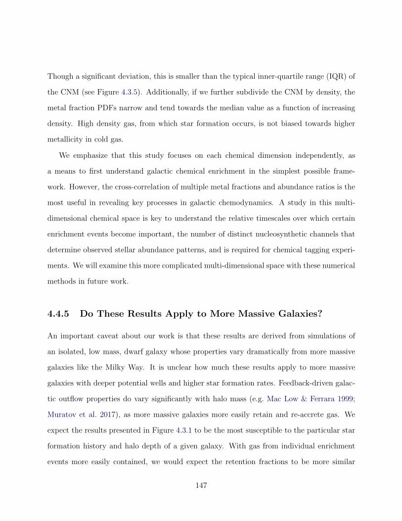
Though a significant deviation, this is smaller than the typical inner-quartile range (IQR) of
the CNM (see Figure 4.3.5). Additionally, if we further subdivide the CNM by density, the
metal fraction PDFs narrow and tend towards the median value as a function of increasing
density. High density gas, from which star formation occurs, is not biased towards higher
metallicity in cold gas.
We emphasize that this study focuses on each chemical dimension independently, as
a means to first understand galactic chemical enrichment in the simplest possible frame-
work. However, the cross-correlation of multiple metal fractions and abundance ratios is the
most useful in revealing key processes in galactic chemodynamics. A study in this multi-
dimensional chemical space is key to understand the relative timescales over which certain
enrichment events become important, the number of distinct nucleosynthetic channels that
determine observed stellar abundance patterns, and is required for chemical tagging experi-
ments. We will examine this more complicated multi-dimensional space with these numerical
methods in future work.
4.4.5 Do These Results Apply to More Massive Galaxies?
An important caveat about our work is that these results are derived from simulations of
an isolated, low mass, dwarf galaxy whose properties vary dramatically from more massive
galaxies like the Milky Way. It is unclear how much these results apply to more massive
galaxies with deeper potential wells and higher star formation rates. Feedback-driven galac-
tic outflow properties do vary significantly with halo mass (e.g. Mac Low & Ferrara 1999;
Muratov et al. 2017), as more massive galaxies more easily retain and re-accrete gas. We
expect the results presented in Figure 4.3.1 to be the most susceptible to the particular star
formation history and halo depth of a given galaxy. With gas from individual enrichment
events more easily contained, we would expect the retention fractions to be more similar
147

Figure 4.4.2: The separation (in dex) of each star’s oxygen fraction from the median valueof the CNM oxygen mass fraction PDF for the time within 1 Myr (our time resolution) ofeach star’s formation time. The median deviation is given in the plot for stars formed afterthe initial star formation and enrichment period (120 Myr.)
148

across metal species with increasing halo mass or decreasing star formation rate. We antic-
ipate three potential regimes of metal retention, depending on dark matter halo mass and
SFR: i) at very low halo mass, even below that examined here, there is equally poor reten-
tion of metal enrichment from both AGB stars and SNe, ii) AGB enrichment is preferentially
retained, but SN enrichment is ejected efficiently (as is the case in this study), and iii) both
sources are well retained in the galaxy’s ISM. If true, this difference in metal retention can be
a key observable in verifying our result that the dynamical evolution of metals in the ISM is
not uniform. This difference would be greater at later times, once AGB enrichment becomes
significant. We would expect dwarf galaxies to exhibit larger abundance ratios between AGB
wind elements and SN enriched elements than stars in more massive galaxies, like the Milky
Way.
In contrast, we expect the properties of the enrichment PDFs, and the variations between
AGB enriched elements and SN enriched elements (as presented in Figures 4.3.4 and 4.3.5),
to be general. We expect metals to exhibit log-normal + power-law distributions in the ISM
of all galaxies, with similar trends with enrichment source and gas phase as outlined here.
However, the detailed properties of the PDFs (e.g, log-normal width, power-law slope) likely
depend non-trivially on global galaxy properties. How these results vary as a function of
galaxy properties will be investigated in future work.
4.4.6 Implications for Exotic Enrichment Sources
We have shown that the dynamical evolution of metals depends upon their nucleosynthetic
source, focusing here on AGB synthesized elements and SN synthesized elements. How-
ever, these differences should also apply to exotic enrichment sources, such as hypernovae,
neutron-star neutron-star mergers, and neutron-star black-hole mergers. These sources can
have energies that differ significantly from typical SNe, reaching > 1052 erg for hypernovae
149

(Nomoto et al. 2004), for example. In addition, these events are rare. For example, neutron
star mergers occur at a rate of approximately 10−5 per M−1� of star formation in the Milky
Way(Kim et al. 2015). This rarity could significantly influence the typical ISM environments
into which they eject their metals. We would therefore expect different mixing behaviors
for metals synthesized through these channels as compared to SNe. Based on our results
here, for example, we would expect elements from hypernovae to be more well mixed in the
ISM of all galaxies, but more readily ejected in dwarf galaxies, as compared to elements
from SNe. Depending on their injection energy, neutron star mergers could exhibit different
mixing behaviors in the ISM. These differences could provide important signatures for dis-
tinguishing individual, exotic enrichment sources from observed stellar abundance patterns
in our own Milky Way and in nearby dwarf galaxies. In particular, low mass dwarf galaxies
with unusual (compared to Milky Way, solar abundances) r-process enrichment (e.g. Ji et al.
2016a; Duggan et al. 2018; Ji et al. 2019), are valuable for constraining the source of these
elements, their frequency, and typical yields. The differential metal evolution presented in
our work both opens up an additional avenue by which elements from distinct nucleosyn-
thetic sources may be distinguished in observations and challenges current assumptions used
in interpreting these observations.
4.4.7 Individual Stars vs. Averaged Yields
Typical models for chemical enrichment in galaxy-scale simulations apply some form of
IMF-averaged nucleosynthetic yields. Unfortunately, it is beyond the scope of this work
to investigate how our results might change when adopting an IMF-averaged yield model.
However, to what degree stochastic IMF sampling, mass-dependent nucleosynthetic yields,
and the dynamical decoupling of individual enrichment sources play in galactic chemical
evolution are valuable questions to address in future research. We speculate that an IMF-
150

averaged enrichment model will only capture the differences between enrichment sources seen
here if the model: 1) captures a multi-phase, turbulent ISM, 2) accounts for the energetic
differences between yields from different enrichment sources, and 3) accounts for the time-
delay between different enrichment sources. Models which average over an entire stellar
population and ignore these effects may be unable to reproduce our results.
4.5 Conclusions
We present a detailed analysis of galactic chemodynamics and metal mixing on an element-
by-element basis in a low mass dwarf galaxy with hydrodynamics simulations that simul-
taneously capture multi-channel stellar feedback in detail with a multi-phase ISM. This
high resolution simulation, coupled with our star-by-star modeling of stellar nucleosynthetic
yields, has allowed us to analyze for the first time how individual metal species couple to
the ISM and galactic wind of this galaxy.
We find that individual metal species do not share the same dynamical evolution, with
differences directly related to nucleosynthetic origin (AGB winds, winds from massive stars,
or core collapse SNe). This difference is most significant, in our model, between elements
ejected predominately by AGB winds and those ejected predominantly by core-collapse SNe.
In addition, we find the novel result that the mass fraction PDFs of each metal in the ISM
can be described using an analytic piecewise log-normal + power-law PDF. The properties of
these PDFs vary with both ISM phase and metal species, again driven mostly by differences
in enrichment sources.
We summarize our results as follows:
• Power-law tails on log-normal metal fraction PDFs are a natural consequence of ongo-
ing chemical enrichment, with the power-law slope related to the rate at which mixing
151

dilutes newly enriched gas.
• Hotter phases have metal fraction PDFs that are more enriched, with significant power-
law tails as compared to cold phases, which have a more prominent log-normal compo-
nent. The lack of significant tails in the cold-phase PDFs indicates that metal mixing
occurs rapidly in hotter phases before cooling and/or mixing into denser gas.
• Metal outflow in low mass dwarf galaxies depends upon nucleosynthetic site. Metals
from lower energy enrichment events (e.g. AGB winds) are preferentially retained in
the ISM as compared to those from higher energy events (e.g. SNe). The degree to
which this is true likely depends upon global galaxy properties such as star formation
rate, dark matter potential well, and gas geometry.
• Likewise, metals originating in AGB winds are less well mixed in the ISM, with spreads
of over 1 dex in cold gas, as compared to metals injected through SNe, with spreads of
about 0.5 dex
• Metal distributions exhibit positive skew, such that the mean metal fraction can be
anywhere from 0.1 to 1.0 dex above the median metal fraction. Simple chemical evo-
lution models, which generally follow the mean abundance, and thus can not account
for complex metal mixing physics, are likely biased towards higher enrichment values.
Extending these results to low-mass dwarf galaxies in general, we expect that: 1) s-
process elements from AGB winds should exhibit larger spreads than α elements released
through SNe and 2) these elements should be overabundant in dwarf galaxies at fixed age,
as compared to massive galaxies like the Milky Way.
152

Acknowledgements
A.E. is funded by the NSF Graduate Research Fellowship DGE 16-44869. G.L.B. is funded by
NSF AST-1312888, NASA NNX15AB20G, and NSF AST-1615955. M.-M.M.L. was partly
funded by NASA grant NNX14AP27G and by NSF grant AST18-15461. B.C. acknowl-
edges support from the ERC Consolidator Grant (Hungary) funding scheme (project RA-
DIOSTAR, G.A. n. 724560) and from the National Science Foundation (USA) under grant
No. PHY-1430152 (JINA Center for the Evolution of the Elements). B.W.O was supported
in part by NSF grants PHY-1430152 and AST-1514700, by NASA grants NNX12AC98G, and
NNX15AP39G, and by Hubble Theory Grant HST-AR-14315.001-A. We gratefully recognize
computational resources provided by NSF XSEDE through grant number TGMCA99S024,
the NASA High-End Computing Program through the NASA Advanced Supercomputing
Division at Ames Research Center, Columbia University, and the Flatiron Institute. This
work made significant use of many open source software packages, including yt, Enzo,
Grackle, Python, IPython, NumPy, SciPy, Matplotlib, HDF5, h5py, Astropy,
Cloudy and deepdish. These are products of collaborative effort by many independent
developers from numerous institutions around the world. Their commitment to open science
has helped make this work possible.
4.A Density PDF
We show the density PDF in Figure 4.A.1 to illustrate our result in comparison to comparable
works that have computed the density PDF in global galaxy simulations with a multi-phase
ISM (Joung et al. 2009; Tasker & Tan 2009; Tasker 2011; Tasker et al. 2015; Hopkins et al.
2012). We show the mass-weighted PDF (dm/Md log n) on the left, and the volume-weighted
153
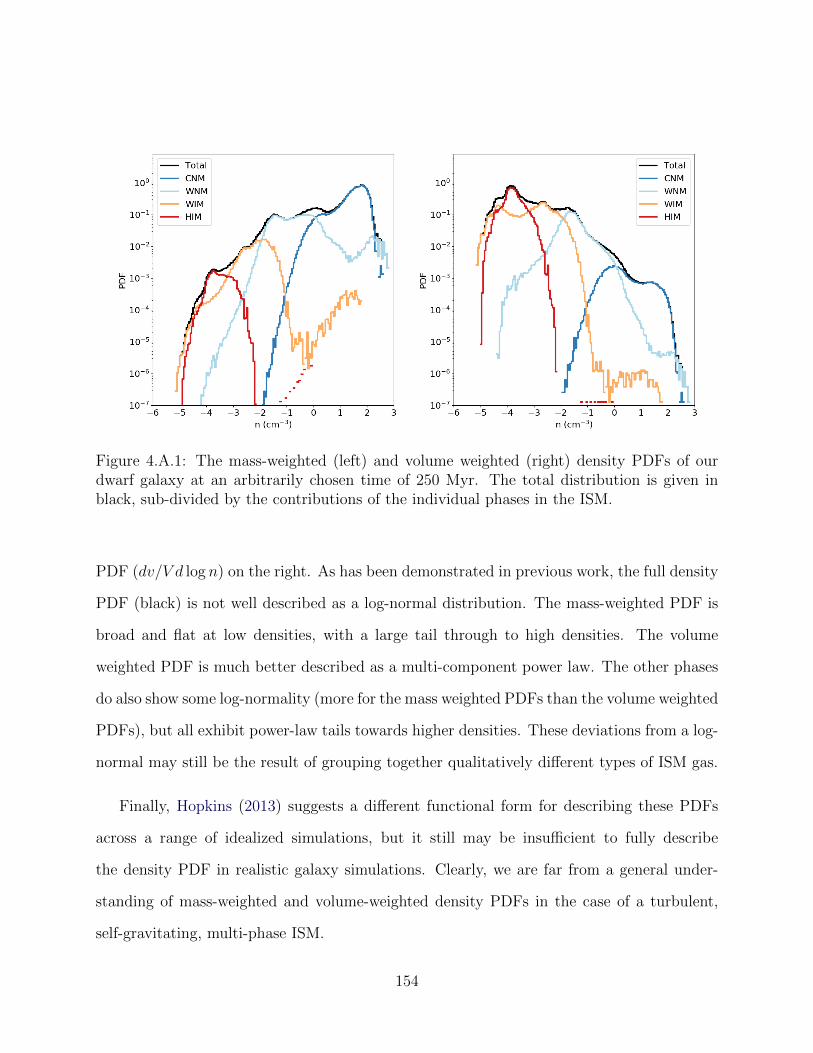
Figure 4.A.1: The mass-weighted (left) and volume weighted (right) density PDFs of ourdwarf galaxy at an arbitrarily chosen time of 250 Myr. The total distribution is given inblack, sub-divided by the contributions of the individual phases in the ISM.
PDF (dv/V d log n) on the right. As has been demonstrated in previous work, the full density
PDF (black) is not well described as a log-normal distribution. The mass-weighted PDF is
broad and flat at low densities, with a large tail through to high densities. The volume
weighted PDF is much better described as a multi-component power law. The other phases
do also show some log-normality (more for the mass weighted PDFs than the volume weighted
PDFs), but all exhibit power-law tails towards higher densities. These deviations from a log-
normal may still be the result of grouping together qualitatively different types of ISM gas.
Finally, Hopkins (2013) suggests a different functional form for describing these PDFs
across a range of idealized simulations, but it still may be insufficient to fully describe
the density PDF in realistic galaxy simulations. Clearly, we are far from a general under-
standing of mass-weighted and volume-weighted density PDFs in the case of a turbulent,
self-gravitating, multi-phase ISM.
154
4.B Resolution Comparison
We perform a resolution test to confirm that the key results of this study are convergent,
at least qualitatively. Given the variations in star formation rate, feedback effectiveness,
and stochasticity in our model, we do not expect exact numerical convergence in any one
quantity. We conduct two lower resolution simulations with a maximum physical resolution
of 3.6 pc and 7.2 pc. We refer the reader to Paper I for a previous comparison of these
simulations to our fiducial run. In Figure 4.B.1 we demonstrate that O and Ba abundances
behave qualitatively similar in our lower resolution runs as in our fiducial model. In both
lower resolution runs O has a generally tighter distribution that narrows over time, while
Ba is much less well mixed, in agreement with our fiducial simulation. The exact numerical
values for these spreads are not convergent across simulations, but we do note significant
variations in the exact SFH of these lower resolution runs could be driving these differences.
155
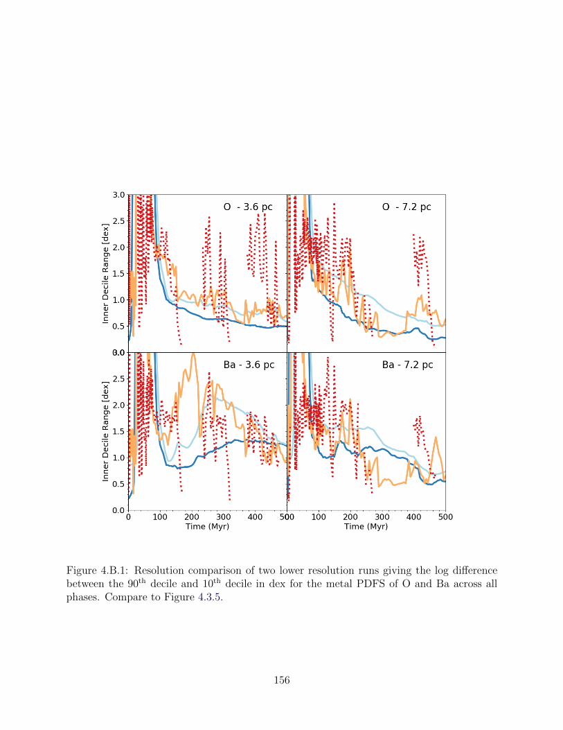
Figure 4.B.1: Resolution comparison of two lower resolution runs giving the log differencebetween the 90th decile and 10th decile in dex for the metal PDFS of O and Ba across allphases. Compare to Figure 4.3.5.
156
Chapter 5
Mixing Properties of Individual
Enrichment Sources
5.1 Introduction
The elemental abundances of a galaxy over time are sensitive to the nuclear physics and
stellar astrophysics that determines which stars make what elements and when. The stellar
abundance patterns within a given galaxy also depend on the details of how those metals
are released into the ISM through various forms of stellar feedback, and the hydrodynamic
interactions that ultimately mix those elements into the ISM or eject them from the galaxy
in galactic winds. Stellar abundance patterns in old, metal poor systems are the result of
enrichment from substantially fewer sources than younger, more metal rich stellar popula-
tions. Because of this, studying abundance patterns in these environments allows us to place
constraints on the yields of individual enrichment events and the nucleosynthetic sites of
each element. The lowest mass dwarf galaxies in the Local Group, UFDs, offer some of the
This section contains unpublished work-in-progress
157

best constraints on these processes. These environments can potentially be used to trace and
constrain enrichment from the first stars (e.g. Frebel & Bromm 2012; Ji et al. 2015; Ritter
et al. 2015; Jeon et al. 2017; Hartwig et al. 2018) and have been used to place constraints on
the variety of possible astrophysical sources of r-process enrichment (e.g. Ji et al. 2016b,c; Ji
& Frebel 2018; Ji et al. 2019; Tsujimoto et al. 2017; Duggan et al. 2018; Nagasawa et al. 2018;
Ojima et al. 2018). It is likely that chemical enrichment in more massive, metal rich systems
with ongoing star formation like the Milky Way exhibits smaller abundance spreads. The
size of more massive galaxies reduces the relevance of stochasticity, averaging over the variety
of complex hydrodynamics and feedback-driven turbulence that may be driving much of the
variance in stellar abundances seen at low metallicity. Stochasticity, which has been shown
to be important for setting the width of stellar abundance patterns in low metallicity envi-
ronments of the Milky Way halo (e.g. Cescutti 2008; Cescutti & Chiappini 2014), plays an
even greater role in the evolution of these low mass dwarf galaxies (Applebaum et al. 2018).
Indeed the increase in scatter in the stellar abundance patterns of low mass dwarf galaxies
and UFDs has been attributed to inhomogeneous mixing and stochastic effects (e.g. Norris
et al. 2010; Lee et al. 2013; Simon et al. 2015; Mashonkina et al. 2017; Suda et al. 2017).
This complicates the interpretation of abundance patterns in these galaxies, particularly for
constraining individual enrichment events.
Recent cosmological zoom simulations have attained sufficient resolution to follow the
evolution of individual UFDs (or their progenitors at high redshift) and can investigate their
chemical properties (Jeon et al. 2017; Corlies et al. 2018; Escala et al. 2018; Christensen
et al. 2018). Additional works have conducted more direct investigations into what drives
the enrichment process for individual sources using both hydrodynamics simulations (Pan
et al. 2013; Ritter et al. 2015; Safarzadeh & Scannapieco 2017; Hirai et al. 2015; Hirai &
Saitoh 2017; Emerick et al. 2018b; Haynes & Kobayashi 2019) and semi-analytic models
158

(Beniamini et al. 2018; Krumholz & Ting 2018). In Emerick et al. (2018b) we demonstrate
that elements released through AGB winds have both wider abundance distributions in the
ISM and lower ejection fractions from the galaxy than elements released in supernovae. In
spite of this progress, there is still substantial work to be done in understanding the physical
processes that drive both evolution of both the mean and width of stellar abundances in
low-mass dwarf galaxies.
In this Chapter we utilize the simulations analyzed in prior chapters to conduct a con-
trolled set of “mixing experiments” whereby we restart each simulation with enrichment
events placed by-hand in order to more directly investigate the evolution of metals from
an individual event. While elemental yields were tracked for each star in our simulation,
we lacked the necessary Lagrangian information1 about the metals once they were released
into the ISM to be able to trace the evolution of single enrichment events. We investigate
primarily how the feedback ejection energy of individual sources (Eej) and global star for-
mation rate at the time of enrichment affects how metals are ejected from the galaxy in
galactic winds and metal mixing in the ISM. In Section 5.2 we briefly outline our methods
and discuss the setup of these mixing experiments. In Section 5.3 we discuss the results of
these experiments and the role of Eej, global SFR, radial position of the enrichment event,
and local ISM density around each enrichment sources affects the evolution of its metals,
and discuss and conclude in Section 5.4.
5.2 Methods
We refer the reader to the previous chapters for more detailed descriptions of our numerical
methods and feedback models. The mixing experiments discussed below are conducted in
1The history of a given fluid element, which is followed natively in SPH codes, but not in the grid-basedhydrodynamics simulations used here.
159
restarted versions of the same low-mass, isolated galaxy simulations used throughout this
work.
5.2.1 Mixing Experiment Setup
We restart our fiducial, full-physics simulation at two different times, 180 Myr, and 360 Myr,
labeled as runs I and II respectively. These correspond to two different times in the galaxy’s
SFR evolution, testing how much variance is expected in the metal mixing and ejection with
the star formation rate. Run I occurs during the lull in star formation following the initial
SFR peak, and run II occurs in an extended period of little to no ongoing star formation. We
attempted to to evolve each simulation for 150 Myr, but due to computational constraints
this was not always possible.2
At the beginning of each restart, we place by-hand one or more enrichment events at
assigned positions throughout the galaxy, with thermal injection energies (Eej), masses (mej),
and metal fractions (Zej). We note that the injection masses, particularly the metal fractions,
are somewhat arbitrary. The injected metal masses are dynamically insignificant relative to
the ambient ISM mass in which they occur; these fields, therefore, act as tracers and do not
impact the dynamics or cooling physics of the simulations. The important parameter here is
Eej, which we vary to sample the range of ejection energies associated with significant sources
of chemical enrichment, including AGB winds (1046 erg)3, NS-NS mergers (1049 − 1050 erg),
supernovae (1051 erg), and exotic enrichment sources, such as hypernovae, that can reach
much higher energies (1052 erg). Each run contains only sources from a single event type, as
indicated in the run-name by the log of the injection energy in ergs. For example, the run
beginning at 180 Myr with AGB-like events is labeled “I E46”. The metal enrichment from
2We began runs during the peak of star formation (∼ 100 Myr), but the computational cost increasessubstantially during this time. These runs were abandoned.
3Assuming full thermalization of the total mechanical energy output of an AGB wind.
160
each source is tracked and evolved with a unique passive scalar tied to the individual source
and separate from any additional chemical enrichment that may occur within the galaxy
over time.
Each run contains multiple events spread over the galaxy to test how radial and azimuthal
position in the galaxy affects mixing and ejection, but limited to ensure that the events do
not overlap and influence each other dynamically. For the low-energy events, we are able to
run 19 events per restart, while the 1049 − 1051 erg runs contain 7 events, and the 1052 erg
runs only contain a single event.
Most of this analysis refers to these average behavior of the metals from these enrichment
events over time as a way to gain a general appreciation for how Eej and galactic properties
affect the evolution of metals. However, we do note that this is not fair statistically, as the
higher energy runs are undersampled.
5.3 Results
Perhaps the three most important parameters to quantify for each enrichment event are: 1)
what fraction of released metals are immediately available for star formation, 2) how does this
fraction evolve over time as metals cool from hot phases into star forming gas, and 3) what
fraction of metals are carried out of the galaxy in outflows. We discuss each of these points
in Section 5.3.1, focusing on the average behavior of multiple enrichment events at fixed
ejection energy. In Section 5.3.2 we go further and address the relative homogeneity (over
time) of the metals retained by the ISM for each enrichment source. Finally, in Section 5.3.3
we discuss how these parameters vary with individual events, and, in Sections 5.3.4 through
5.3.6, how they vary with radial position in the galaxy, ISM properties in the event region,
and global galaxy SFR.
161

5.3.1 Enrichment of the ISM and CGM
We summarize the source-averaged results for all enrichment events in runs I E46, I E49,
I E50, I E51, and I E52 in Figure 5.3.1 by showing the fraction of source metals contained
within each phase of the ISM (colored lines, which sum to the black dashed line), and the
CGM (black, solid). These plots show a clear, immediate trend across Eej for all lines
in the figure, but the differences are most striking for the ISM (black, dashed) and CGM
(black, solid) lines. In Chapter 4 we demonstrated that there was a significant difference
in metal ejection fraction, fej, for metals from AGB sources as compared to metals released
in SNe. Here, we confirm that this is driven predominantly by differences in the energy
of the events, and not necessarily when or where they occur in the ISM. The clear trend
in Figure 5.3.1 shows that events with higher Eej are much more readily ejected from the
disk of the galaxy, while events with lower Eej couple poorly to the same galactic outflows.
The high-energy events rapidly converge on a peak fej within about 20 Myr of the event,
with only a gradual increase towards the end of the 150 Myr as the metals in the ISM are
swept up in additional outflows. The lower energy events evolve more gradually. The lowest
energy event, corresponding to AGB winds, reaches fej ∼ 0.68, which increases to 0.87 for
the 1051 erg events, and 0.95 for the 1052 erg event. To emphasize these differences, we plot
each line separately in the left panel of Figure 5.3.2
This implies that, if one to were assume that all metals behaved the same and adopted
an fej of ∼0.9 – typical for the total metal ejection fraction in simulations that do not
track individual enrichment channels (e.g. Muratov et al. 2017; Christensen et al. 2018), and
consistent with observations of the O abundance in Local Group dwarf galaxies (e.g. Kirby
et al. 2011c; McQuinn et al. 2015b) – one would underestimate the amount of AGB metals
in the ISM by a factor of ∼ 3, and overestimate exotic, high-energy sources by a factor
162

Figure 5.3.1: Time evolution of the fraction of metals in each phase of the ISM (coloredlines; CNM: dark blue, WNM: light blue, WIM: orange, HIM: red), the galaxy’s disk (black,dashed), and the CGM (black, solid) as averaged across all events at a given Eej. Thefractions are all normalized to the total amount of metals initially injected in each event.The individual ISM phases sum to the black, dashed line.
163

of ∼ 2. In each case, these are metals that cannot participate in the enrichment of future
stellar populations and will make a significant difference to the output stellar abundances in
chemical evolution models.
In all cases, the metals contained within the ISM are deposited predominantly in the
ionized phases of the ISM, the WIM or the HIM, with the relative fraction in each phase
driven by the energy of the event. Metals in the ISM injected with Eej > 1049 erg are
initially located predominately in the HIM, roughly 1/2 for Eej = 1049 erg and nearly all for
Eej > 1051 erg. The lowest energy events are initially in the WIM and WNM, tracing the
two dominant volume-filling components of the ISM (see Chapter 2), as these events do not
have sufficient energy to generate the HIM by themselves.
Gas above the star formation threshold in our simulations is limited and short-lived due
to the low gas surface densities and star formation rates in this galaxy and the efficiency
of stellar feedback from newly formed stars. As a proxy, we examine the evolution of the
CNM, out of which the star forming gas forms. In general, very few of these elements are
available for immediate star formation in the CNM (<< 1%, see Figure 5.3.2). However, we
note that we may not have sufficient resolution to properly resolve the details of the initial
mixing of individual enrichment events in the ISM. In addition, this value will be sensitive to
whether or not a given event occurs in the vicinity of or inside an active, star forming region
– as is likely for core collapse SNe, and unlikely for other events. Thus, this is a quantity
that does not depend solely on Eej and is sensitive to whether or not self-enrichment of star
forming regions is an important factor in galactic chemical evolution. We are also missing
important physical processes, like dust production in AGB winds and core collapse SNe,
that may affect these results for specific enrichment channels in ways that do not depend
solely on Eej. Investigating the fraction of metals immediately available for star formation
will require additional, high-resolution simulations of metal mixing in and around individual
164

star forming regions. This will be useful for understanding stellar enrichment patterns that
may arise from star formation in regions whose metal abundance patters arise directly from
unmixed ejecta of a single enrichment source.
What we can examine, however, is the final quantity of interest: the long-term evolution
of the metals from each of these sources, and how long it takes for these metals to propagate
from the warm / hot phases of the ISM to cold, star forming gas. In the right panel of
Figure 5.3.2, we examine the evolution of the metal fraction of the CNM for just those
elements retained in the ISM. Although the initial CNM fractions are about the same for
each source, the evolution over the first ∼50 Myr is qualitatively different. The higher energy
sources, Eej > 1049 erg, are more rapidly incorporated into the CNM than E46, even though
each retains a lower fraction of metals in the ISM. This is most significant at ∼20 Myr, when
the fraction of metals in the CNM from these sources is a factor of ∼3-4 higher than the E46
metals. By ∼50 Myr, the evolutions become intermingled and complex, with no clear trend
as a function of Eej.
However, the metals from each source do gradually trend towards a fraction of ∼0.8 by
the end of the 150 Myr simulation time. This value corresponds to the total mass fraction of
the CNM (see Figure 2.6). This trend – that the fraction of metals contained in a given phase
tends towards the mass fraction of that phase – is true across all phases in the simulation.
Therefore, we can consider that the metals for each source are well-mixed across the phases
of the ISM on timescales of ∼100-150 Myr. This is comparable to, but less than, the
dynamical timescale of the galaxy, ∼200 Myr. These two results suggest that the delay-time
between when metals are available to enrich ongoing star formation is on order of ∼10 Myr
across sources, and only significant for the lowest (E46, AGB-like) energy sources. Although
well-mixed across phases, we emphasize that this does not imply that the abundances are
the same across phases nor that the metals are spatially well-mixed across the galaxy. We
165

Figure 5.3.2: Time evolution of the fraction of enrichment source metals contained in theCGM over time (left), and the fraction of metals in the CNM relative to just those metalsretained in the ISM for each enrichment source (right). These are the same as the linesin Figure 5.3.1, but the CNM lines are normalized by the black, dashed total ISM line inFigure 5.3.1.
investigate this second point further below.
5.3.2 Homogeneity of Mixing
In Chapter 4 we investigate the metal enrichment distributions in the ISM as characterized
by the metal fraction PDFs (see Figure 4.3.4 and Figure 4.3.5). We find that this PDF is
generally well described as log-normal with a power law tail towards high metal fractions,
and characterize its mean, median, interquartile range (IQR), interdecile range (IDR), and
the difference between the mean and median (as a measure of skew) of each distribution. In
general, we find that elements released in AGB-wind events are less well-mixed than elements
released in SNe, as indicated by the relative size of the IQR, IDR, and mean-median difference
between the two types of elements. However, these distributions arise from the contribution
of many individual enrichment events across multiple sources over long periods of time. It is
166
unclear how metals from a single enrichment event are distributed across a galaxy over time,
and how the energy associated with the event affects the homogeneity of its distribution.
To frame this analysis, let us first examine what processes affect the metal mass fraction
PDF. The mean metal mass fraction for a collection of gas is simply the total metal mass
divided by the total gas mass. For a collection of gas elements, the mean metal mass fraction
is defined as Zgas = ΣZiMgas,i/ΣMgas,i, where Mgas,i is the mass of the ith homogeneous blob of
gas, and Zi its metal mass fraction. A completely homogeneous ISM would have a δ function
metal mass fraction PDF at the mean metal fraction, or p(Z) = δ(Zgas). By definition, then,
a homogeneous distribution will have a zero-width IQR, IDR, and mean-median difference.
Non-uniform enrichment in a homogeneous medium will increase each of these quantities,
while mixing in a non-uniform medium will tend to decrease each. In simple models of
galactic chemical evolution, the mean gas abundance – not the median – is followed, even
though the median is more indicative of the abundance of a “typical” gas element. Because
these two quantities provide a more immediate conceptual understanding of how metals are
distributed in the ISM, we focus on characterizing the inhomogeneity of the followed metals
by examining the mean-median difference. Though it is necessary for this quantity to be
zero for metals to be homogeneously distributed in a medium, we do note that it is not a
sufficient condition (the mean of a symmetric distribution is equal to the median). However,
its evolution is easy to interpret conceptually. Enrichment increases this quantity by raising
the mean metal fraction while keeping the median value fixed (or only slightly increasing),
so long as the newly enriched mass is a small fraction of the total gas mass (as is almost
always the case). Conversely, preferential removal of metals from a medium will lower this
quantity. And finally, the mixing of metal-rich gas elements with metal-poor will gradually
bring the mean and median values to parity. For our numerical experiments, enrichment in
the whole ISM only occurs once and ejection from the ISM is easy to follow. This allows for
167

Figure 5.3.3: Time evolution of the difference (in dex) between the mean metal mass fractionof each source and the median metal mass fraction of each source in all of the gas in the ISM(left) and in the CNM only (right).
a cleaner interpretation of the evolution than examining either the IQR or the IDR.
In Figure 5.3.3 we examine the average behavior of the mean-median metal mass fractions
for the whole ISM in each run (left) and the CNM only (right). In all cases, enrichment
drives the dramatic increase of this value from zero to over 10 dex. This large value is due
entirely because the initial abundance for each metal is near zero and thus a majority of the
gas (by mass) is at an arbitrarily small metal mass fraction. This is followed by a significant
decrease in spread over the first 25 Myr or so as metals are preferentially ejected from the
ISM via outflows. The delay in this spike in the CNM (compared to the galaxy as a whole)
is due to the different timescales over which most of the metals are incorporated into the
cold gas, as shown in Figure 5.3.1.
Clearly, at no point can any of these distributions be considered well-mixed within the
150 Myr simulation time. Prior studies of passive scalar mixing in isothermal turbulent
168
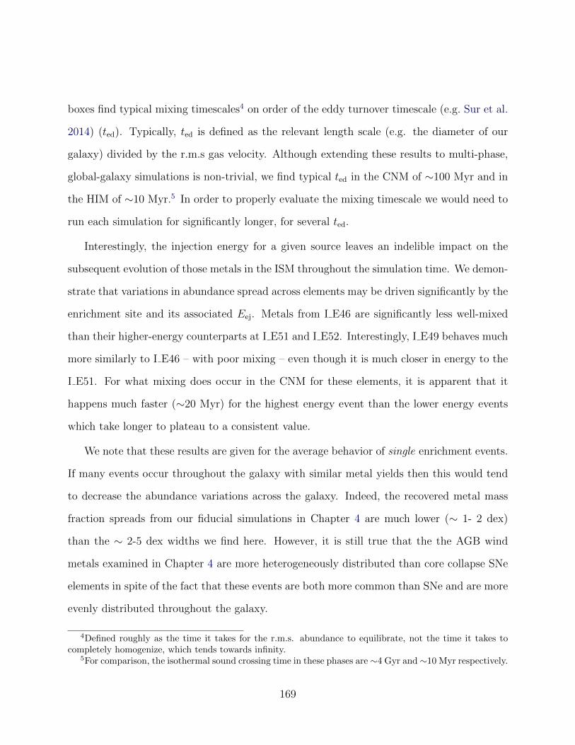
boxes find typical mixing timescales4 on order of the eddy turnover timescale (e.g. Sur et al.
2014) (ted). Typically, ted is defined as the relevant length scale (e.g. the diameter of our
galaxy) divided by the r.m.s gas velocity. Although extending these results to multi-phase,
global-galaxy simulations is non-trivial, we find typical ted in the CNM of ∼100 Myr and in
the HIM of ∼10 Myr.5 In order to properly evaluate the mixing timescale we would need to
run each simulation for significantly longer, for several ted.
Interestingly, the injection energy for a given source leaves an indelible impact on the
subsequent evolution of those metals in the ISM throughout the simulation time. We demon-
strate that variations in abundance spread across elements may be driven significantly by the
enrichment site and its associated Eej. Metals from I E46 are significantly less well-mixed
than their higher-energy counterparts at I E51 and I E52. Interestingly, I E49 behaves much
more similarly to I E46 – with poor mixing – even though it is much closer in energy to the
I E51. For what mixing does occur in the CNM for these elements, it is apparent that it
happens much faster (∼20 Myr) for the highest energy event than the lower energy events
which take longer to plateau to a consistent value.
We note that these results are given for the average behavior of single enrichment events.
If many events occur throughout the galaxy with similar metal yields then this would tend
to decrease the abundance variations across the galaxy. Indeed, the recovered metal mass
fraction spreads from our fiducial simulations in Chapter 4 are much lower (∼ 1- 2 dex)
than the ∼ 2-5 dex widths we find here. However, it is still true that the the AGB wind
metals examined in Chapter 4 are more heterogeneously distributed than core collapse SNe
elements in spite of the fact that these events are both more common than SNe and are more
evenly distributed throughout the galaxy.
4Defined roughly as the time it takes for the r.m.s. abundance to equilibrate, not the time it takes tocompletely homogenize, which tends towards infinity.
5For comparison, the isothermal sound crossing time in these phases are ∼4 Gyr and ∼10 Myr respectively.
169

What this does suggest, however, is that in utilizing stars with unusual abundances at low
metallicities to infer the yields of exotic enrichment sources, the spread of abundances in those
stars may provide an important insight into the origin of those metals. For example, r-process
enrichment from exotic enrichment events like hypernovae should manifest itself as more
well-mixed than if the elements originated in lower energy NS-NS mergers. Conducting this
analysis requires measured r-process abundances for a large sample of stars in an individual
dwarf galaxy. This is challenging for the lowest mass, most metal poor dwarf galaxies, which
typically only have a few to 10 stars with measured abundances, but could be done for low
mass dwarfs like Ursa Minor, for more massive dwarfs like Carina, and Fornax (Suda et al.
2017), and for the low-metallicity stellar halo of the Milky Way (e.g. Hansen et al. 2018;
Sakari et al. 2018).
5.3.3 Event-by-Event Variation
For clarity we have focused on the mean evolution of individual enrichment events at fixed
injection energy in the results thus far. We turn now to discuss how much variety exists
among these individual events. For each of the discussed runs (from set I), Figure 5.3.4
shows the fraction of event tracer metals ejected from the galaxy (left) and the fraction of
metals in the ISM within the CNM (center) as a function of source energy at two different
times, 20 Myr (blue) and 100 Myr (orange). In the right panel, we show how the spread at
each of these times varies for each event. The averaged values at each energy are shown as
points, and the bars denote the min/max value for each event energy.6 As shown, there is
substantial variation at each energy. This is particularly striking for the E46 events, which
seemingly can have any value of fCGM and fCNM/fDisk at any point during the evolution.
6While the standard deviation or IQR may be more informative here, rather than min / max, the samplesize at each energy, with the exception of the E46 runs, is too small to reliably do so.
170
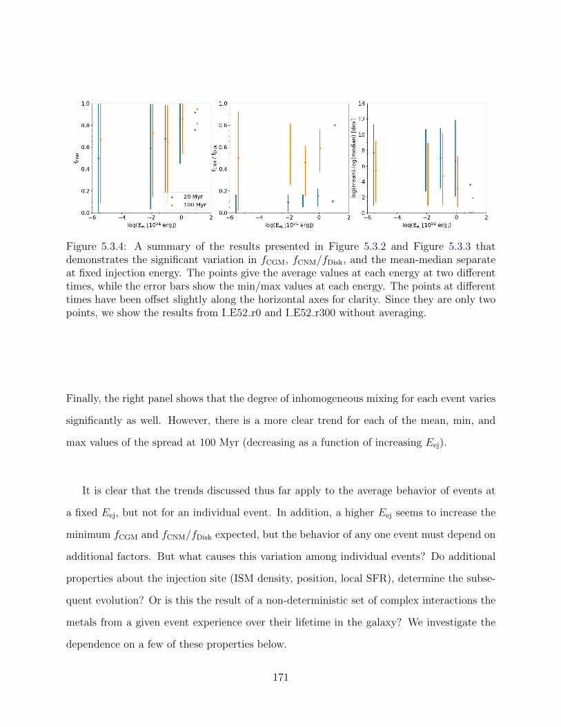
Figure 5.3.4: A summary of the results presented in Figure 5.3.2 and Figure 5.3.3 thatdemonstrates the significant variation in fCGM, fCNM/fDisk, and the mean-median separateat fixed injection energy. The points give the average values at each energy at two differenttimes, while the error bars show the min/max values at each energy. The points at differenttimes have been offset slightly along the horizontal axes for clarity. Since they are only twopoints, we show the results from I E52 r0 and I E52 r300 without averaging.
Finally, the right panel shows that the degree of inhomogeneous mixing for each event varies
significantly as well. However, there is a more clear trend for each of the mean, min, and
max values of the spread at 100 Myr (decreasing as a function of increasing Eej).
It is clear that the trends discussed thus far apply to the average behavior of events at
a fixed Eej, but not for an individual event. In addition, a higher Eej seems to increase the
minimum fCGM and fCNM/fDisk expected, but the behavior of any one event must depend on
additional factors. But what causes this variation among individual events? Do additional
properties about the injection site (ISM density, position, local SFR), determine the subse-
quent evolution? Or is this the result of a non-deterministic set of complex interactions the
metals from a given event experience over their lifetime in the galaxy? We investigate the
dependence on a few of these properties below.
171
5.3.4 Dependence on Radial Position
We place each source at regular, but arbitrary, positions in the galaxy without consideration
for the local ISM conditions at injection. Sources are placed at the center of the galaxy
(r = 0 pc) or at various radii (at cardinal positions at 300 pc, and 600 pc), all in the mid-
plane of the galaxy. Since the E46 events were likely to not self-interact, we additionally
placed events at r = 100 pc and one event at each r at about one scale height above the disk
(z = 50 pc). For each I run, we plot fCGM and fCNM/fDisk as a function of radial position in
the galaxy for each event in Figure 5.3.5. The points, error bars, and colors are the same as
in Figure 5.3.4.
Across runs, there is no clear dependence on the radial position of the event and the
fraction of metals ejected beyond the galaxy for any of the displayed runs at either 20 Myr
or 100 Myr. There is a slight increase in the minimum fraction of metals ejected from the
galaxy as a function of radius for the higher energy runs (> 1050 erg). This is perhaps not
surprising for the largest radii as 600 pc is right near the very edge of the galaxy’s disk. But
again, the trend is weak and there is clearly still a great variance at both fixed Eej and r.
The fraction of metals in the ISM that are contained within the CNM (middle row) does not
show any obvious trend at E46, but does seem to generally be lowest for the higher energy
sources at the outskirts of the galaxy. Finally, the radial position does seem to affect the
mixing behavior. Sources at the outskirts of the galaxy tend to be more inhomogeneous than
sources at inner radii, especially at 20 Myr for the higher energy events, and the variation
in behavior for these sources decreases substantially, particularly at 100 Myr. It is unclear
what exactly drives these mixing differences. If feedback-driven turbulence is the dominant
driver of ISM mixing in this dwarf galaxy – as it likely is – then sources near the center are
more likely to be affected by more feedback events (due to a slightly higher ΣSFR) and mix
172
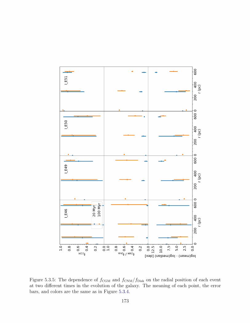
Figure 5.3.5: The dependence of fCGM and fCNM/fDisk on the radial position of each eventat two different times in the evolution of the galaxy. The meaning of each point, the errorbars, and colors are the same as in Figure 5.3.4.
173

more efficiently.
5.3.5 Variation with Local ISM Conditions
We compute the average ISM properties within a 4-zone radius (4 × dx = 7.2 pc) around
each injection site to examine any potential correlations in evolution with ISM properties.7
In Figure 5.3.6 we plot fCGM and fCNM/fDisk for each I run as a function of the average
number density (< n >) in the injection region within 0.1 Myr (our time resolution) of
the event. The E46 events clearly do a better job sampling the ISM density PDF, with
a slight trend of decreasing fCGM (more retained metals) with local ISM number density.
This difference is even true after 100 Myr of evolution, but still with significant variation
at fixed n. The number statistics limit a conclusive result for the higher energy events, but
generally there does not appear to be an obvious trend in behavior of fCGM as a function of
n. This is perhaps because these energies are sufficient to heat up and dramatically reduce
the density of the ISM in the injection region regardless of n. This is not the case for the
E46 events. fCNM/fDisk does not display any significant variation with n at 100 Myr, but is
slightly elevated at 20 Myr at higher densities. There is still a variety of behavior at fixed
n. Finally, we note no obvious trends of the spread of the metal PDFs as a function of n for
all but the E46 run. Again, the local ISM densities are likely not too dynamically relevant
to the higher energy events – hence their lack of variation with n – but this is not true for
E46. There is a fairly clear trend of increasing inhomogeneity in the CNM as a function of
the initial n in the injection region for E46, that is not present at 20 Myr, but is obvious at
100 Myr.
7Note that the injection region for each event is a 3-cell radius sphere mapped onto the grid with a CICinterpolation scheme.
174
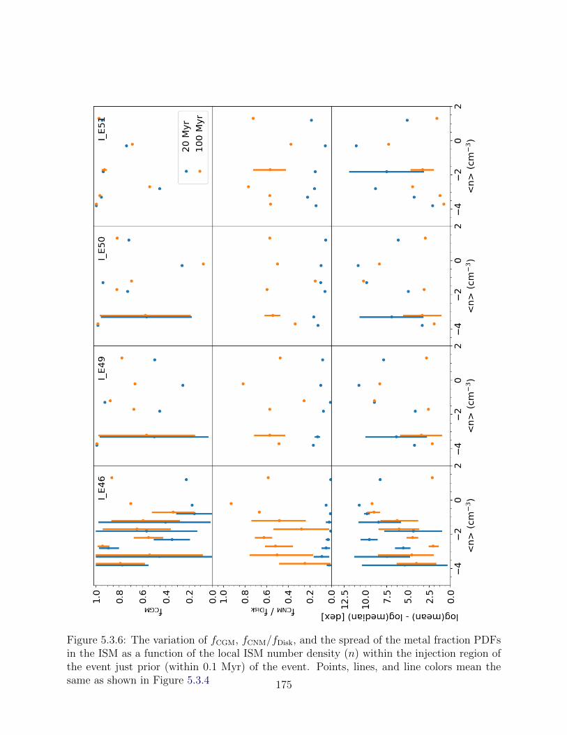
Figure 5.3.6: The variation of fCGM, fCNM/fDisk, and the spread of the metal fraction PDFsin the ISM as a function of the local ISM number density (n) within the injection region ofthe event just prior (within 0.1 Myr) of the event. Points, lines, and line colors mean thesame as shown in Figure 5.3.4 175

5.3.6 Variation with SFR
Finally, we examine the companion run (II) to see if the global star formation rate of the
galaxy drives variation in these results. Although this does not help to directly account
for the variation seen in the previous plots, this could provide insight into how SFR (in
an averaged sense) affects the evolution of metals. We note that correlation with SFR is
of interest not because the formation of stars by themselves affects metal evolution, but
rather the increase in feedback associated with a higher SFR (and thus a warmer / hotter
ISM, greater turbulence in the ISM, and more significant outflows). We compare these
two runs in Figure 5.3.7, showing runs from I in green and runs at the lower SFR, II, in
purple. fCGM increases much more rapidly across injection energies in I. However, this value
seems to be similar across runs for E49 and E51 by ∼50 Myr, with an additional increase
again in the I simulations towards the end of the time. This initial spike, lull, and second
increase corresponds to the period of active star formation, slightly lull, and increase in SFR
experienced during the I simulations (see Figure 2.4; the lull occurs between 40 and 80 Myr
after the enrichment events, or during 220 - 260 Myr in that figure). The SFR is consistently
low (or zero) throughout II, with just a couple brief increases in SFR. Although E49 and E51
exhibit similar behavior across global differences in SFR, the difference in E46 is significant
throughout the examined time period. As these sources do not contain enough energy to
eject their metals from the galaxy by themselves, they are only ejected from the galaxy by
being swept up in the ISM during other feedback events. The evolution of these events are
therefore much more dependent upon the global galaxy properties.
The fraction of metals contained within the CNM of the ISM does not seem to depend
too strongly on the SFR, unlike fCGM. It is generally true that after the initial ∼50 Myr of
enrichment, a greater fraction of the metals in the ISM are contained in the CNM during
176

the run with the lower SFR (II), but this difference is not large and is only significant for
the higher energy events. In addition, the mass fraction of the CNM is greater during run
II than in run I, so it may simply be that the long-term evolution of the fraction of metals
in the CNM is more dependent upon the phase structure of the ISM – which is regulated by
stellar feedback – than the feedback directly.
Finally, examining the last panel of Figure 5.3.7, it does appear that the mixing efficiency
of metals for each source increases with increasing global SFR. In the initial evolution, all
events in run II exhibit larger abundance spreads that take longer to begin mixing sub-
stantially than their counterparts in I. In general, II abundances remain larger for the first
100 Myr. The differences depend on the ejection energy, with the most significant difference
found in comparing the E46 runs.
5.4 Discussion and Conclusions
Galactic chemical evolution is far from “one-zone” and metal mixing is clearly neither homo-
geneous nor instantaneous. As demonstrated in Chapter 4 and as found in the analytic work
of Krumholz & Ting (2018), the properties of metal mixing in the ISM of various galaxies
depend upon the characteristics of the individual sources – namely the energy with which
they eject metals into the ISM. This sets the thermal phase to which these metals couple
to most effectively, and the volume over which they are initially injected before additional
mixing by global galactic dynamics begins to dominate. In short, lower energy enrichment
events, like those from AGB winds, mix much more slowly throughout the ISM than metals
from higher energy events, like supernovae. As found in Chapter 4, this difference is still
present even when accounting for the fact that AGB events are both more common and
evenly distributed in the galaxy than SNe. In the new work discussed in this chapter, we
177

Figure 5.3.7: The same as Figure 5.3.2, but comparing across both sets of runs with differentSFRs. Comparing across line colors for a fixed linestyle compares the difference the globalSFR has on the average enrichment evolution for both fCGM and fCNM/fDisk.
178

further explore this behavior to try and determine the evolution of individual enrichment
sources – rather than just the average behavior of many sources – and to explore how Eej,
radial position in the galaxy, local ISM density, and global galaxy SFR affect the evolution
of these metals.
We confirm the average trends found in previous works that sources with lower Eej have
larger abundance spreads in the ISM and lower ejection fractions, on average. In addition,
we find that Eej of the event and the global SFR during the time at which the event occurs
produce the greatest variation in how many metals are retained by the galaxy, what fraction
of those metals are contained within the CNM, and their homogeneity. Metals are in general
ejected more effectively and mix more efficiently during periods of higher SFR than low,
corresponding to periods of more effective galactic outflows and greater turbulence in the
ISM. Although we have limited statistics to determine a conclusive trend, we generally find
that the radial position at which the event occurs and the local ISM density in which the
event occurs to not have a significant effect on the average behavior of enrichment events,
with the exception of the lower energy (E46) events. However, we find these results to only be
loose trends about the average behavior of enrichment sources. The evolution of individual
events can be dramatically different, even at fixed energy and global galaxy SFR.
Variations with individual events in the above results suggests that it would be challeng-
ing to make any conclusive statements about the enrichment behavior of single enrichment
sources. This is problematic for interpreting the chemical abundances in UFDs that are
likely to have been host to just a single, exotic enrichment event. Using these observations
to constrain the total nucleosynthetic yields of these sources requires implicit assumptions
about how quickly metals are available in star forming gas, how homogeneously they are
distributed throughout the galaxy, and what fraction are ejected from the galaxy. It is
likely that none of these quantities can be determined as simple parameters based upon the
179

feedback properties of a single enrichment source or even the global properties of a galaxy
(such as Mhalo, ΣSFR, Σgas). However, this study has shown that these parameters can be
characterized in an averaged sense, even though the exact result is subject to substantial
stochastic effects. This, combined with some mechanism to provide this stochasticity, can
be used in combination with many runs of a simple galactic chemical evolution model to
understand the possible outcomes for various galaxies. Developing such a model will be a
powerful tool for interpreting the irregular stellar abundance patterns observed in low mass
dwarf galaxies in the nearby Universe.
180

Chapter 6
Conclusion
This Dissertation has focused on building an understanding of galactic chemical evolution
with the point of view that the same feedback processes that regulate star formation and
drive galactic winds in galaxies also play a fundamental role in their metal enrichment. It is
understood that stellar feedback plays an important role in driving metals out into the CGM
around galaxies and beyond, but the exact coupling of metals to galactic winds is not well
understood. This is in part because how metals mix within a multi-phase ISM to eventually
be swept up in galactic outflows or mix within cold, star forming gas is not well constrained.
Even more, how metals from the full range of nucleosynthetic sources, including AGB winds,
stellar winds, core collapse and Type Ia supernovae, and NS-NS mergers, participate in
these processes – mixing and galactic winds – differently has only recently been examined
in efforts to better understand results from the ever increasing availability of high-quality
stellar abundance measurements of stars in our own Milky Way and in nearby dwarf galaxies.
In order to build a complete picture of metal evolution in the Universe, we have developed
a new model for star formation, stellar feedback, and chemical enrichment to follow these
processes in simulations of isolated dwarf galaxies. Using this model, we have made critical
181
advancements in understanding both how stellar feedback governs the evolution of low mass
dwarf galaxies and how individual metals are distributed in (and beyond) these galaxies over
time. We summarize these results below, and conclude with a discussion of future research.
6.1 A New Model for Galactic Chemical Enrichment
In order to address these outstanding issues in galactic evolution, we developed a new model
for galactic chemical evolution that – for the first time in galaxy-scale simulations – follows
star particles as individual stars along with their detailed feedback and metal yields. As
detailed in Chapter 3 we use the AMR hydrodynamics code Enzo to produce a set of
simulations using this model of an idealized, isolated low-mass dwarf galaxy (Mgas ∼ 106 M�,
Mhalo ∼ 3 × 10⁹ M�) embedded in a static dark matter potential. Using a detailed model
for gas chemistry and radiative cooling, we follow the evolution of this galaxy and its multi-
phase ISM as it forms stars, depositing individual star particles sampled over 1 to 100 M�.
We follow the feedback processes from each of these stars, including the AGB winds from
low mass stars, Lyman-Werner radiation, FUV radiation (and photoelectric heating), and
ionizing radiation from massive stars, and both core collapse and Type Ia supernovae. We
track the metal yields for each of these stars, following 15 individual metal species as they
mix within the ISM and imprint their abundances onto the sites of future star formation or
are ejected from the galaxy altogether.
We find that this model – which contains no independently tuned free parameters – is
sufficient to generate a multi-phase ISM with star formation, gas scale-height, and outflow
properties that match expectations from observations. The global metal retention fraction
for this galaxy is low (. 5%), with typical outflow velocities of ∼100 km s−1, and up to
1000 km s−1. We find that stellar radiation feedback is important, but that the ISRF is
182
highly variable – driven by stochastic IMF sampling in this low SFR galaxy. The mass
fraction of the ISM is dominated by the cold (T∼100 K) and warm-neutral (T∼1000 K)
components, while the warm-ionized and hot phases dominated the volume fraction. The
WIM and HIM in the galaxy also exhibit significant time variation due to stochastic IMF
sampling and a bursty SFH. Finally, we find that H2 comprises . 5% of the galaxy by mass,
formed primarily through H− gas-phase reactions.
6.2 Stellar Radiation Feedback in Dwarf Galaxies
Stellar radiation has recently been invoked as an important source of feedback – in addition
to supernovae – that helps to regulate star formation and drive galactic winds in galaxies
across the mass scale. This feedback channel acts immediately after the formation of massive
stars and is thus an important source of pre-SN feedback. In addition to destroying cold gas
in star forming regions, this acts to dramatically reduce the typical ISM densities in which
SNe explode, increasing their impact. Modeling stellar radiation in galaxies in detail can be
computationally expensive, with a variety of approximate methods available to reduce this
expense. In our simulations we track the ionizing radiation from massive stars accurately
using an adaptive ray-tracing radiative transfer method with sufficient resolution to capture
the HII regions from individual stars. In Chapter 3 we demonstrate that stellar ionizing ra-
diation dramatically reduces the star formation rate and generally increases the effectiveness
of galactic winds in our low-mass dwarf galaxy simulations.
In addition, we explore the mechanism by which stellar radiation acts to regulate star
formation and drive outflows by comparing our fiducial simulations to simulations that only
account for localized (< 20 pc) ionization around massive stars. This second set of runs
mimics the behavior of various approximations for stellar radiation feedback which do not
183

follow radiation propagation in detail, but rather deposit energy / ionize gas in the immediate
vicinity of newly formed stars. We find that star formation is regulated by ionizing radiation
locally – destroying cold gas around young, massive stars that would otherwise have formed
stars – as the < 20 pc restricted run (initially) shares a very similar SFR to our fiducial run.
However, we find that these simulations exhibit dramatically different outflow properties,
which drive long-term differences in galactic properties including SFR and metal retention.
Stellar radiation at larger distance scales is important for carving out diffuse channels of gas
in the ISM and into the CGM of our dwarf galaxy through which SNe can effectively blow
out mass and metals from the ISM. This suggests that – at least in low mass dwarf galaxies
– localized approximations of radiation feedback are likely insufficient for capturing the full
effects of stellar radiation.
6.3 Mixing and Ejection of Individual Metals
As argued in Krumholz & Ting (2018), differences in how metals are released into the
ISM (due to the variation in energetics between their nucleosynthetic sites) should drive
discernible differences in their mixing behavior in the ISM. We demonstrate these differences
for the first time in hydrodynamics simulations in Chapter 4 by examining the evolution of
each of the 15 metals species tracked in our simulations. Although we are not the first to
follow a large number of individual metal species from different nucleosynthetic channels in
a galaxy-scale simulation, that we follow individual stars and follow the feedback for each
independently has allowed us to capture these effects. Notably, we find that – for low mass
dwarf galaxies – metals released in AGB winds are retained in the galaxy’s ISM at a much
higher fraction than metals released in either core collapse or Type Ia supernovae. This
implies that if one were to construct a chemical evolution model of a low mass dwarf galaxy
184

and adopt the high metal ejection fractions as seen in observations1 (Kirby et al. 2011b;
McQuinn et al. 2015b), one could underestimate the mass of AGB-wind dominated metals
(such as Sr and Ba, and possibly C and N) in the ISM by a factor of ∼ 4-5. This effect is
important in matching observations of stellar abundances in low mass dwarf galaxies, but
how this ratio depends on galaxy properties (e.g. M∗, Mhalo, ΣSFR, Σgas) is uncertain and
warrants future research.
In agreement with predictions from Krumholz & Ting (2018), we find that the abun-
dances of the AGB-wind metals are more inhomogeneous than the abundances of metals
from supernovae. This spread can be significant, over 1 dex for the AGB-wind elements. We
predict then that – at least in the low metallicity environments of low mass dwarf galaxies
– the observed stellar abundance distributions for AGB-wind elements should be character-
ized by markedly greater spreads than abundance distributions for SNe elements (e.g. O,
Mg). Indeed, this is observed in the stellar abundance patterns of dwarf galaxies in the
Local Group (Suda et al. 2017), but it remains to be seen if this is a conclusive signature of
these mixing differences or perhaps is due to larger differences in star-to-star metal yields for
these elements. Finally, we were able to characterize the metal mass fraction PDFs for each
element across each phase of the ISM, and found that they generically well-fit by a combined
log-normal PDF with a power-law tail towards higher metal mass fractions. We hope that
this characterization lends itself well to developing a physically-motivated semi-analytic pre-
scription for stellar abundance spreads to be used in semi-analytic (and one-zone) models of
galactic chemical evolution.
1Which typically trace O, an element released predominately in core collapse supernovae.
185

6.4 Mixing Behavior of Single-Sources
To expand upon the results of Chapter 4 and understand how metals are distributed through-
out the ISM on a source-by-source level, we carry out a series of “mixing experiments” in
Chapter 5 to test how metal mixing and metal ejection behaviors vary with the injection
energy of the source. We confirm that lower energy events (e.g. AGB-winds) are retained at
a higher fraction in the ISM and mix poorly compared to higher energy events (e.g. SNe) on
average. We demonstrate this by following the evolution of metals of individual sources at
injection energies of 1046 erg (AGB winds), 1049 erg and 1050 erg (NS-NS mergers), 1051 erg
(SNe and possibly NS-NS mergers), and 1052 erg (hypernovae). However, we find that the
behavior of any single source exhibits a substantial amount of variance – particularly at
lower energies – as it is clear that the injection energy is not the only dominant factor in
determining mixing behavior. We investigate other possible factors, including radial posi-
tion, global galaxy SFR, and local ISM density, and find that the global galaxy SFR has
the greatest effect on the mixing and ejection behavior of each metal, particularly for lower
energy events. While these results suggest that these behavioral differences can be accounted
for in an average sense, the full picture is subject to substantial stochasticity based purely
on the randomness with which both when and where different events occur in a galaxy.
Abundances associated with rare enrichment sources – such as the r-process enrichment can-
didates – which may only occur once (if at all) in the lowest mass dwarf galaxies should
therefore exhibit the most significant galaxy-to-galaxy abundance variations for galaxies at
fixed stellar mass.
186

6.5 Future Work
One of the primary goals of this Dissertation was to develop a physical understanding of the
processes that contribute generally to galactic chemical evolution and specifically to metal
mixing and ejection from galaxies – a process that was previously not well understood. With
a novel model for star formation and stellar feedback we have made substantial contributions
to this understanding, but continued work is necessary. Specifically, the conclusions reached
in this Dissertation have all been made in the context of the evolution of a low-mass dwarf
galaxy with idealized initial conditions and limited cosmological context. Although we can
speculate, it remains to be seen how these results can vary over cosmological timescales for
a single galaxy as well as how they vary across the galaxy mass scale. Besides conducting
a suite of simulations sampling a variety of galaxy parameters, which could prove too com-
putationally expensive at higher galaxy masses, semi-analytic and one-zone models provide
the ideal testing ground for identifying what regimes may be sensitive to the metal mixing
behaviors identified in this work. The ultimate goal would be to use a suite of hydrodynamics
simulations to construct physically motivated prescriptions for use in these one-zone models.
Until then, however, future work can make significant strides with the results presented here
alone.
To aid in this development, we have built a one-zone model, OneZ, that has been designed
to match the physical model used in our hydrodynamics simulations.2. This model uses an
equivalent star formation recipe as our hydrodynamics simulations, stochastically forming
individual star particles and following their yields. Given an input SFH and fej for each metal
from our hydrodynamics simulations, we can match the mean metal abundance evolution
from these simulations and can explore how varying fej (element-by-element) affects the
2https://github.com/aemerick/OneZ
187

resultant stellar abundance patterns. In future work, we plan to implement a two-phase
model like that in Schonrich & Weinberg (2019) that includes parameters for how each
metal first enters the hot and cold phases, how each metal mixes between the two phases,
and a stochastic mixing-zone method as used in Cescutti (2008). With these additions,
we will: 1) explore how these physics manifest themselves in galaxies with a wide range
of star formation and halo properties, 2) use these insights to begin to match observed
stellar abundance patterns in low-mass dwarf galaxies, 3) make predictions for expected
multi-element abundance spreads in dwarf galaxies for comparison to future observations in
upcoming surveys, and 4) better constrain the relative importance of stochastic sampling of
the IMF and inhomogeneous mixing in setting these abundance spreads. In addition, we can
more easily use this model to explore a wide variety of nucleosynthetic yield tables to better
constrain the – highly uncertain – yields themselves. These insights can be used to improve
more complex chemical evolution models that account for the cosmological and hierarchical
evolution of galaxies over time. This is a particularly exciting tool that can be used to better
constrain the sources of r-process enrichment in low mass dwarf galaxies.
In addition, this work can be readily extended to further investigate how feedback governs
the evolution of dwarf galaxies. We have already produced a suite of comparison simulations
at a factor two lower resolution (3.6 pc) than our fiducial resolution, turning on and off each
individual feedback process to understand the significance and characterize the mechanism
by which each operates to regulate star formation and drive galactic winds. The feedback
tested here includes supernovae, stellar ionizing radiation, photoelectric heating, Lyman-
Werner radiation, and radiation pressure. The suite contains simulations including “all-
but-one” of each process, in addition to several combinations where multiple effects are
excluded, and a set where the effectiveness of radiation pressure is artificially increased and
decreased. Comparing the evolution of these dwarfs to our fiducial simulations presented in
188

this Dissertation will improve our understanding of these processes, building upon previous
works that have conducted similar studies in more massive dwarf galaxies (Hu et al. 2016,
2017; Forbes et al. 2016; Hopkins et al. 2018). Our unique contribution to this field will be
in examining how these processes change how metals are retained / ejected by galactic winds
and mix within the ISM.
Finally, in ongoing work we are implementing these methods in zoom-in cosmological sim-
ulations of UFD galaxy evolution. Our detailed model tracking the feedback and yields from
individual stars will build substantially upon recent works investigating metal enrichment
at high redshift and in UFDs and their progenitors (e.g. Ritter et al. 2015; Jeon et al. 2017;
Corlies et al. 2018; Wheeler et al. 2018; Agertz et al. 2019). This work includes additional
improvements to the simulations presented in this Dissertation, including a model for Pop
III star formation and chemical enrichment adapted from Wise et al. (2012b), a new IMF
sampling scheme that allows us to follow very low mass stars (M∗ . 2 M�) – which have
no significant feedback or metal enrichment, but are important long-lived tracers of galactic
chemical enrichment – aggregated together into a single particle during each star forma-
tion event, improvements to the numerical implementation to ease memory consumption in
these significantly larger simulations, and new metal tracer fields to follow the contribution
of AGB, core collapse SNe, Type Ia SNe, and PopIII stars to the total metal content of
each cell independently. This will provide a more direct, fundamental test of the underlying
physics that governs galactic evolution and produce simulated galaxies that can be more
readily compared to observations of nearby dwarf galaxies.
189
Bibliography
Abbott, D. C. 1982, ApJ, 263, 723
Abramson, L. E., Gladders, M. D., Dressler, A., Oemler, Jr., A., Poggianti, B., & Vulcani,
B. 2016, ApJ, 832, 7
Agertz, O. & Kravtsov, A. V. 2015, ApJ, 804, 18
Agertz, O., Kravtsov, A. V., Leitner, S. N., & Gnedin, N. Y. 2013, ApJ, 770, 25
Agertz, O., Moore, B., Stadel, J., Potter, D., Miniati, F., Read, J., Mayer, L., Gawryszczak,
A., Kravtsov, A., Nordlund, A., Pearce, F., Quilis, V., Rudd, D., Springel, V., Stone, J.,
Tasker, E., Teyssier, R., Wadsley, J., & Walder, R. 2007, MNRAS, 380, 963
Agertz, O., Pontzen, A., Read, J. I., Rey, M. P., Orkney, M., Rosdahl, J., Teyssier, R.,
Verbeke, R., Kretschmer, M., & Nickerson, S. 2019, arXiv e-prints
Amorın, R., Munoz-Tunon, C., Aguerri, J. A. L., & Planesas, P. 2016, A&A, 588, A23
Anders, F., Chiappini, C., Santiago, B. X., Rocha-Pinto, H. J., Girardi, L., da Costa, L. N.,
Maia, M. A. G., Steinmetz, M., Minchev, I., Schultheis, M., Boeche, C., Miglio, A.,
Montalban, J., Schneider, D. P., Beers, T. C., Cunha, K., Allende Prieto, C., Balbinot,
E., Bizyaev, D., Brauer, D. E., Brinkmann, J., Frinchaboy, P. M., Garcıa Perez, A. E.,
Hayden, M. R., Hearty, F. R., Holtzman, J., Johnson, J. A., Kinemuchi, K., Majewski,
190
S. R., Malanushenko, E., Malanushenko, V., Nidever, D. L., O’Connell, R. W., Pan, K.,
Robin, A. C., Schiavon, R. P., Shetrone, M., Skrutskie, M. F., Smith, V. V., Stassun, K.,
& Zasowski, G. 2014, A&A, 564, A115
Andrews, B. H. & Martini, P. 2013, ApJ, 765, 140
Andrews, B. H., Weinberg, D. H., Schonrich, R., & Johnson, J. A. 2017, ApJ, 835, 224
Angles-Alcazar, D., Faucher-Giguere, C.-A., Keres, D., Hopkins, P. F., Quataert, E., &
Murray, N. 2017, MNRAS, 470, 4698
Applebaum, E., Brooks, A. M., Quinn, T. R., & Christensen, C. R. 2018, arXiv e-prints
Armillotta, L., Krumholz, M. R., & Fujimoto, Y. 2018, MNRAS, 481, 5000
Artale, M. C., Tissera, P. B., & Pellizza, L. J. 2015, MNRAS, 448, 3071
Asplund, M., Grevesse, N., Sauval, A. J., & Scott, P. 2009, ARA&A, 47, 481
Aubert, D., Deparis, N., & Ocvirk, P. 2015, MNRAS, 454, 1012
Baczynski, C., Glover, S. C. O., & Klessen, R. S. 2015, MNRAS, 454, 380
Bakes, E. L. O. & Tielens, A. G. G. M. 1994, ApJ, 427, 822
Belfiore, F., Maiolino, R., Tremonti, C., Sanchez, S. F., Bundy, K., Bershady, M., Westfall,
K., Lin, L., Drory, N., Boquien, M., Thomas, D., & Brinkmann, J. 2017, MNRAS, 469,
151
Beniamini, P., Dvorkin, I., & Silk, J. 2018, MNRAS, 478, 1994
Bergin, E. A., Hartmann, L. W., Raymond, J. C., & Ballesteros-Paredes, J. 2004, ApJ, 612,
921
191

Bernstein-Cooper, E. Z., Cannon, J. M., Elson, E. C., Warren, S. R., Chengular, J., Skillman,
E. D., Adams, E. A. K., Bolatto, A. D., Giovanelli, R., Haynes, M. P., McQuinn, K. B. W.,
Pardy, S. A., Rhode, K. L., & Salzer, J. J. 2014, AJ, 148, 35
Bland-Hawthorn, J., Karlsson, T., Sharma, S., Krumholz, M., & Silk, J. 2010a, ApJ, 721,
582
Bland-Hawthorn, J., Krumholz, M. R., & Freeman, K. 2010b, ApJ, 713, 166
Bland-Hawthorn, J., Sutherland, R., & Webster, D. 2015, ApJ, 807, 154
Bleuler, A. & Teyssier, R. 2014, MNRAS, 445, 4015
Bordoloi, R., Tumlinson, J., Werk, J. K., Oppenheimer, B. D., Peeples, M. S., Prochaska,
J. X., Tripp, T. M., Katz, N., Dave, R., Fox, A. J., Thom, C., Ford, A. B., Weinberg,
D. H., Burchett, J. N., & Kollmeier, J. A. 2014, ApJ, 796, 136
Bouche, N., Dekel, A., Genzel, R., Genel, S., Cresci, G., Forster Schreiber, N. M., Shapiro,
K. L., Davies, R. I., & Tacconi, L. 2010, ApJ, 718, 1001
Bradford, J. D., Geha, M. C., & Blanton, M. R. 2015, ApJ, 809, 146
Bressan, A., Marigo, P., Girardi, L., Salasnich, B., Dal Cero, C., Rubele, S., & Nanni, A.
2012, MNRAS, 427, 127
Brook, C. B., Stinson, G., Gibson, B. K., Shen, S., Maccio, A. V., Obreja, A., Wadsley, J.,
& Quinn, T. 2014, MNRAS, 443, 3809
Bryan, G. L. & Norman, M. L. 1998, ApJ, 495, 80
Bryan, G. L., Norman, M. L., O’Shea, B. W., Abel, T., Wise, J. H., Turk, M. J., Reynolds,
D. R., Collins, D. C., Wang, P., Skillman, S. W., Smith, B., Harkness, R. P., Bordner, J.,
192

Kim, J.-h., Kuhlen, M., Xu, H., Goldbaum, N., Hummels, C., Kritsuk, A. G., Tasker, E.,
Skory, S., Simpson, C. M., Hahn, O., Oishi, J. S., So, G. C., Zhao, F., Cen, R., Li, Y., &
The Enzo Collaboration. 2014, ApJS, 211, 19
Bryan, G. L., Norman, M. L., Stone, J. M., Cen, R., & Ostriker, J. P. 1995, Computer
Physics Communications, 89, 149
Buder, S., Asplund, M., Duong, L., Kos, J., Lind, K., Ness, M. K., Sharma, S., Bland-
Hawthorn, J., Casey, A. R., De Silva, G. M., D’Orazi, V., Freeman, K. C., Lewis, G. F.,
Lin, J., Martell, S. L., Schlesinger, K. J., Simpson, J. D., Zucker, D. B., Zwitter, T.,
Amarsi, A. M., Anguiano, B., Carollo, D., Casagrande, L., Cotar, K., Cottrell, P. L., Da
Costa, G., Gao, X. D., Hayden, M. R., Horner, J., Ireland, M. J., Kafle, P. R., Munari, U.,
Nataf, D. M., Nordlander, T., Stello, D., Ting, Y.-S., Traven, G., Watson, F., Wittenmyer,
R. A., Wyse, R. F. G., Yong, D., Zinn, J. C., & Zerjal, M. 2018, MNRAS, 478, 4513
Bullock, J. S. & Boylan-Kolchin, M. 2017, ARA&A, 55, 343
Burkert, A. 1995, ApJ, 447, L25
Burkhart, B., Falceta-Goncalves, D., Kowal, G., & Lazarian, A. 2009, ApJ, 693, 250
Burkhart, B., Stalpes, K., & Collins, D. C. 2017, ApJ, 834, L1
Cannon, J. M., Giovanelli, R., Haynes, M. P., Janowiecki, S., Parker, A., Salzer, J. J.,
Adams, E. A. K., Engstrom, E., Huang, S., McQuinn, K. B. W., Ott, J., Saintonge, A.,
Skillman, E. D., Allan, J., Erny, G., Fliss, P., & Smith, A. 2011, ApJ, 739, L22
Cescutti, G. 2008, A&A, 481, 691
Cescutti, G. & Chiappini, C. 2014, A&A, 565, A51
193
Ceverino, D., Klypin, A., Klimek, E. S., Trujillo-Gomez, S., Churchill, C. W., Primack, J.,
& Dekel, A. 2014, MNRAS, 442, 1545
Chen, H., Chen, S., & Kraichnan, R. H. 1989, Physical Review Letters, 63, 2657
Chen, H. H.-H., Burkhart, B., Goodman, A., & Collins, D. C. 2018, ApJ, 859, 162
Christensen, C. R., Dave, R., Brooks, A., Quinn, T., & Shen, S. 2018, ArXiv e-prints
Christensen, C. R., Dave, R., Governato, F., Pontzen, A., Brooks, A., Munshi, F., Quinn,
T., & Wadsley, J. 2016, ApJ, 824, 57
Cohen, J. G., Christlieb, N., Thompson, I., McWilliam, A., Shectman, S., Reimers, D.,
Wisotzki, L., & Kirby, E. 2013, ApJ, 778, 56
Colbrook, M. J., Ma, X., Hopkins, P. F., & Squire, J. 2017, MNRAS, 467, 2421
Colella, P. & Woodward, P. R. 1984, Journal of Computational Physics, 54, 174
Collins, D. C., Kritsuk, A. G., Padoan, P., Li, H., Xu, H., Ustyugov, S. D., & Norman, M. L.
2012, ApJ, 750, 13
Corlies, L., Johnston, K. V., & Wise, J. H. 2018, MNRAS, 475, 4868
Cote, B., O’Shea, B. W., Ritter, C., Herwig, F., & Venn, K. A. 2017, ApJ, 835, 128
Cote, B., Ritter, C., O’Shea, B. W., Herwig, F., Pignatari, M., Jones, S., & Fryer, C. L.
2016a, ApJ, 824, 82
Cote, B., Silvia, D. W., O’Shea, B. W., Smith, B., & Wise, J. H. 2018, ApJ, 859, 67
Cote, B., West, C., Heger, A., Ritter, C., O’Shea, B. W., Herwig, F., Travaglio, C., &
Bisterzo, S. 2016b, MNRAS, 463, 3755
194
Cowan, J. J., Sneden, C., Lawler, J. E., Aprahamian, A., Wiescher, M., Langanke, K.,
Martınez-Pinedo, G., & Thielemann, F.-K. 2019, arXiv e-prints
Dale, J. E. & Bonnell, I. A. 2008, MNRAS, 391, 2
Dale, J. E., Ngoumou, J., Ercolano, B., & Bonnell, I. A. 2014, MNRAS, 442, 694
Dave, R., Rafieferantsoa, M. H., Thompson, R. J., & Hopkins, P. F. 2017, MNRAS, 467,
115
de Avillez, M. A. & Mac Low, M.-M. 2002a, ApJ, 581, 1047
—. 2002b, ApJ, 581, 1047
De Silva, G. M., Freeman, K. C., Bland-Hawthorn, J., Martell, S., de Boer, E. W., As-
plund, M., Keller, S., Sharma, S., Zucker, D. B., Zwitter, T., Anguiano, B., Bacigalupo,
C., Bayliss, D., Beavis, M. A., Bergemann, M., Campbell, S., Cannon, R., Carollo, D.,
Casagrande, L., Casey, A. R., Da Costa, G., D’Orazi, V., Dotter, A., Duong, L., Heger,
A., Ireland, M. J., Kafle, P. R., Kos, J., Lattanzio, J., Lewis, G. F., Lin, J., Lind, K.,
Munari, U., Nataf, D. M., O’Toole, S., Parker, Q., Reid, W., Schlesinger, K. J., Sheinis,
A., Simpson, J. D., Stello, D., Ting, Y.-S., Traven, G., Watson, F., Wittenmyer, R., Yong,
D., & Zerjal, M. 2015, MNRAS, 449, 2604
Dekel, A. & Silk, J. 1986, ApJ, 303, 39
Diemer, B., Sparre, M., Abramson, L. E., & Torrey, P. 2017, ApJ, 839, 26
Draine, B. T. 2011, Physics of the Interstellar and Intergalactic Medium
Drlica-Wagner, A., Bechtol, K., Rykoff, E. S., Luque, E., Queiroz, A., Mao, Y.-Y., Wechsler,
R. H., Simon, J. D., Santiago, B., Yanny, B., Balbinot, E., Dodelson, S., Fausti Neto, A.,
195

James, D. J., Li, T. S., Maia, M. A. G., Marshall, J. L., Pieres, A., Stringer, K., Walker,
A. R., Abbott, T. M. C., Abdalla, F. B., Allam, S., Benoit-Levy, A., Bernstein, G. M.,
Bertin, E., Brooks, D., Buckley-Geer, E., Burke, D. L., Carnero Rosell, A., Carrasco Kind,
M., Carretero, J., Crocce, M., da Costa, L. N., Desai, S., Diehl, H. T., Dietrich, J. P.,
Doel, P., Eifler, T. F., Evrard, A. E., Finley, D. A., Flaugher, B., Fosalba, P., Frieman,
J., Gaztanaga, E., Gerdes, D. W., Gruen, D., Gruendl, R. A., Gutierrez, G., Honscheid,
K., Kuehn, K., Kuropatkin, N., Lahav, O., Martini, P., Miquel, R., Nord, B., Ogando, R.,
Plazas, A. A., Reil, K., Roodman, A., Sako, M., Sanchez, E., Scarpine, V., Schubnell, M.,
Sevilla-Noarbe, I., Smith, R. C., Soares-Santos, M., Sobreira, F., Suchyta, E., Swanson,
M. E. C., Tarle, G., Tucker, D., Vikram, V., Wester, W., Zhang, Y., Zuntz, J., & DES
Collaboration. 2015, ApJ, 813, 109
Duggan, G. E., Kirby, E. N., Andrievsky, S. M., & Korotin, S. A. 2018, ArXiv e-prints
Emerick, A., Bryan, G. L., & Mac Low, M.-M. 2018a, ApJ, 865, L22
—. 2019, MNRAS, 482, 1304
Emerick, A., Bryan, G. L., Mac Low, M.-M., Cote, B., Johnston, K. V., & O’Shea, B. W.
2018b, ApJ, 869, 94
Escala, I., Wetzel, A., Kirby, E. N., Hopkins, P. F., Ma, X., Wheeler, C., Keres, D., Faucher-
Giguere, C.-A., & Quataert, E. 2018, MNRAS, 474, 2194
Eswaran, V. & Pope, S. B. 1988, Physics of Fluids, 31, 506
Evans, C. J., Castro, N., Gonzalez, O. A., Garcia, M., Bastian, N., Cioni, M.-R. L., Clark,
J. S., Davies, B., Ferguson, A. M. N., Kamann, S., Lennon, D. J., Patrick, L. R., Vink,
J. S., & Weisz, D. R. 2019, A&A, 622, A129
196

Fabian, A. C. 2012, ARA&A, 50, 455
Farber, R., Ruszkowski, M., Yang, H.-Y. K., & Zweibel, E. G. 2018, ApJ, 856, 112
Faucher-Giguere, C.-A., Keres, D., & Ma, C.-P. 2011, MNRAS, 417, 2982
Federrath, C., Banerjee, R., Clark, P. C., & Klessen, R. S. 2010, ApJ, 713, 269
Federrath, C. & Klessen, R. S. 2013, ApJ, 763, 51
Federrath, C., Klessen, R. S., & Schmidt, W. 2008, ApJ, 688, L79
Feng, Y. & Krumholz, M. R. 2014, Nature, 513, 523
Ferland, G. J., Porter, R. L., van Hoof, P. A. M., Williams, R. J. R., Abel, N. P., Lykins,
M. L., Shaw, G., Henney, W. J., & Stancil, P. C. 2013, Rev. Mexicana Astron. Astrofis.,
49, 137
Ferrara, A. & Tolstoy, E. 2000, MNRAS, 313, 291
Ferrero, I., Abadi, M. G., Navarro, J. F., Sales, L. V., & Gurovich, S. 2012, MNRAS, 425,
2817
Few, C. G., Courty, S., Gibson, B. K., Kawata, D., Calura, F., & Teyssier, R. 2012, MNRAS,
424, L11
Few, C. G., Courty, S., Gibson, B. K., Michel-Dansac, L., & Calura, F. 2014, MNRAS, 444,
3845
Fielding, D., Quataert, E., Martizzi, D., & Faucher-Giguere, C.-A. 2017, MNRAS, 470, L39
Finlator, K. & Dave, R. 2008, MNRAS, 385, 2181
Forbes, J. C., Krumholz, M. R., Goldbaum, N. J., & Dekel, A. 2016, Nature, 535, 523
197
Fragile, P. C., Murray, S. D., & Lin, D. N. C. 2004, ApJ, 617, 1077
Frebel, A. 2018, Annual Review of Nuclear and Particle Science, 68, 237
Frebel, A. & Bromm, V. 2012, ApJ, 759, 115
Frebel, A. & Norris, J. E. 2015, ARA&A, 53, 631
Freeman, K. & Bland-Hawthorn, J. 2002, ARA&A, 40, 487
Fryer, C. L., Belczynski, K., Wiktorowicz, G., Dominik, M., Kalogera, V., & Holz, D. E.
2012, ApJ, 749, 91
Fryxell, B., Olson, K., Ricker, P., Timmes, F. X., Zingale, M., Lamb, D. Q., MacNeice, P.,
Rosner, R., Truran, J. W., & Tufo, H. 2000, ApJS, 131, 273
Gatto, A., Walch, S., Naab, T., Girichidis, P., Wunsch, R., Glover, S. C. O., Klessen, R. S.,
Clark, P. C., Peters, T., Derigs, D., Baczynski, C., & Puls, J. 2017, MNRAS, 466, 1903
Geen, S., Rosdahl, J., Blaizot, J., Devriendt, J., & Slyz, A. 2015, MNRAS, 448, 3248
Geha, M., Blanton, M. R., Masjedi, M., & West, A. A. 2006, ApJ, 653, 240
Geha, M., Blanton, M. R., Yan, R., & Tinker, J. L. 2012, ApJ, 757, 85
Geisler, D., Smith, V. V., Wallerstein, G., Gonzalez, G., & Charbonnel, C. 2005, AJ, 129,
1428
Gilmore, G., Randich, S., Asplund, M., Binney, J., Bonifacio, P., Drew, J., Feltzing, S.,
Ferguson, A., Jeffries, R., Micela, G., & et al. 2012, The Messenger, 147, 25
Giovanelli, R., Haynes, M. P., Adams, E. A. K., Cannon, J. M., Rhode, K. L., Salzer, J. J.,
Skillman, E. D., Bernstein-Cooper, E. Z., & McQuinn, K. B. W. 2013, AJ, 146, 15
198

Giovanelli, R., Haynes, M. P., Kent, B. R., Perillat, P., Saintonge, A., Brosch, N., Catinella,
B., Hoffman, G. L., Stierwalt, S., Spekkens, K., Lerner, M. S., Masters, K. L., Momjian, E.,
Rosenberg, J. L., Springob, C. M., Boselli, A., Charmandaris, V., Darling, J. K., Davies,
J., Garcia Lambas, D., Gavazzi, G., Giovanardi, C., Hardy, E., Hunt, L. K., Iovino, A.,
Karachentsev, I. D., Karachentseva, V. E., Koopmann, R. A., Marinoni, C., Minchin, R.,
Muller, E., Putman, M., Pantoja, C., Salzer, J. J., Scodeggio, M., Skillman, E., Solanes,
J. M., Valotto, C., van Driel, W., & van Zee, L. 2005, AJ, 130, 2598
Girichidis, P., Naab, T., Walch, S., Hanasz, M., Mac Low, M.-M., Ostriker, J. P., Gatto, A.,
Peters, T., Wunsch, R., Glover, S. C. O., Klessen, R. S., Clark, P. C., & Baczynski, C.
2016, ApJ, 816, L19
Gladders, M. D., Oemler, A., Dressler, A., Poggianti, B., Vulcani, B., & Abramson, L. 2013,
ApJ, 770, 64
Glover, S. C., Savin, D. W., & Jappsen, A.-K. 2006, ApJ, 640, 553
Glover, S. C. O. 2003, ApJ, 584, 331
Glover, S. C. O. & Abel, T. 2008, MNRAS, 388, 1627
Glover, S. C. O. & Mac Low, M.-M. 2007, ApJ, 659, 1317
Goldbaum, N. J., Krumholz, M. R., & Forbes, J. C. 2015, ApJ, 814, 131
—. 2016, ApJ, 827, 28
Goldman, S. R., van Loon, J. T., Zijlstra, A. A., Green, J. A., Wood, P. R., Nanni, A.,
Imai, H., Whitelock, P. A., Matsuura, M., Groenewegen, M. A. T., & Gomez, J. F. 2017,
MNRAS, 465, 403
199
Gong, H. & Ostriker, E. C. 2013, ApJS, 204, 8
Gotberg, Y., de Mink, S. E., & Groh, J. H. 2017, A&A, 608, A11
Gotberg, Y., de Mink, S. E., Groh, J. H., Kupfer, T., Crowther, P. A., Zapartas, E., &
Renzo, M. 2018, A&A, 615, A78
Graur, O. & Maoz, D. 2013, MNRAS, 430, 1746
Greco, J. P., Greene, J. E., Strauss, M. A., Macarthur, L. A., Flowers, X., Goulding, A. D.,
Huang, S., Kim, J. H., Komiyama, Y., Leauthaud, A., Leisman, L., Lupton, R. H., Sifon,
C., & Wang, S.-Y. 2018, ApJ, 857, 104
Grudic, M. Y., Hopkins, P. F., Faucher-Giguere, C.-A., Quataert, E., Murray, N., & Keres,
D. 2018, MNRAS, 475, 3511
Haardt, F. & Madau, P. 2001, in Clusters of Galaxies and the High Redshift Universe
Observed in X-rays, ed. D. M. Neumann & J. T. V. Tran, 64
Haardt, F. & Madau, P. 2012, ApJ, 746, 125
Habing, H. J. 1968, Bull. Astron. Inst. Netherlands, 19, 421
Hanasz, M., Lesch, H., Naab, T., Gawryszczak, A., Kowalik, K., & Woltanski, D. 2013, ApJ,
777, L38
Hansen, T. T., Holmbeck, E. M., Beers, T. C., Placco, V. M., Roederer, I. U., Frebel, A.,
Sakari, C. M., Simon, J. D., & Thompson, I. B. 2018, ApJ, 858, 92
Hartwig, T., Yoshida, N., Magg, M., Frebel, A., Glover, S. C. O., Gomez, F. A., Griffen, B.,
Ishigaki, M. N., Ji, A. P., Klessen, R. S., O’Shea, B. W., & Tominaga, N. 2018, MNRAS,
478, 1795
200
Haynes, C. J. & Kobayashi, C. 2019, MNRAS, 483, 5123
Haynes, M. P. 2019, arXiv e-prints
Haynes, M. P., Giovanelli, R., Martin, A. M., Hess, K. M., Saintonge, A., Adams, E. A. K.,
Hallenbeck, G., Hoffman, G. L., Huang, S., Kent, B. R., Koopmann, R. A., Papastergis,
E., Stierwalt, S., Balonek, T. J., Craig, D. W., Higdon, S. J. U., Kornreich, D. A., Miller,
J. R., O’Donoghue, A. A., Olowin, R. P., Rosenberg, J. L., Spekkens, K., Troischt, P., &
Wilcots, E. M. 2011, AJ, 142, 170
Heger, A., Fryer, C. L., Woosley, S. E., Langer, N., & Hartmann, D. H. 2003, ApJ, 591, 288
Hill, V., Skuladottir, A., Tolstoy, E., Venn, K. A., Shetrone, M. D., Jablonka, P., Primas,
F., Battaglia, G., de Boer, T. J. L., Francois, P., Helmi, A., Kaufer, A., Letarte, B.,
Starkenburg, E., & Spite, M. 2018, arXiv e-prints
Hirai, Y., Ishimaru, Y., Saitoh, T. R., Fujii, M. S., Hidaka, J., & Kajino, T. 2015, ApJ, 814,
41
Hirai, Y. & Saitoh, T. R. 2017, ApJ, 838, L23
Hogg, D. W., Casey, A. R., Ness, M., Rix, H.-W., Foreman-Mackey, D., Hasselquist, S., Ho,
A. Y. Q., Holtzman, J. A., Majewski, S. R., Martell, S. L., Meszaros, S., Nidever, D. L.,
& Shetrone, M. 2016, ApJ, 833, 262
Hollenbach, D. & McKee, C. F. 1979, ApJS, 41, 555
Hopkins, P. F. 2013, MNRAS, 430, 1880
—. 2015, MNRAS, 450, 53
201

Hopkins, P. F., Keres, D., Onorbe, J., Faucher-Giguere, C.-A., Quataert, E., Murray, N., &
Bullock, J. S. 2014, MNRAS, 445, 581
Hopkins, P. F., Quataert, E., & Murray, N. 2011, MNRAS, 417, 950
—. 2012, MNRAS, 421, 3488
Hopkins, P. F., Wetzel, A., Keres, D., Faucher-Giguere, C.-A., Quataert, E., Boylan-Kolchin,
M., Murray, N., Hayward, C. C., Garrison-Kimmel, S., Hummels, C., Feldmann, R., Tor-
rey, P., Ma, X., Angles-Alcazar, D., Su, K.-Y., Orr, M., Schmitz, D., Escala, I., Sanderson,
R., Grudic, M. Y., Hafen, Z., Kim, J.-H., Fitts, A., Bullock, J. S., Wheeler, C., Chan,
T. K., Elbert, O. D., & Narananan, D. 2017, ArXiv e-prints
Hopkins, P. F., Wetzel, A., Keres, D., Faucher-Giguere, C.-A., Quataert, E., Boylan-Kolchin,
M., Murray, N., Hayward, C. C., Garrison-Kimmel, S., Hummels, C., Feldmann, R., Tor-
rey, P., Ma, X., Angles-Alcazar, D., Su, K.-Y., Orr, M., Schmitz, D., Escala, I., Sanderson,
R., Grudic, M. Y., Hafen, Z., Kim, J.-H., Fitts, A., Bullock, J. S., Wheeler, C., Chan,
T. K., Elbert, O. D., & Narayanan, D. 2018, MNRAS, 480, 800
Hu, C.-Y. 2018, ArXiv e-prints
Hu, C.-Y., Naab, T., Glover, S. C. O., Walch, S., & Clark, P. C. 2017, MNRAS, 471, 2151
Hu, C.-Y., Naab, T., Walch, S., Glover, S. C. O., & Clark, P. C. 2016, MNRAS, 458, 3528
Hunter, D. A., Ficut-Vicas, D., Ashley, T., Brinks, E., Cigan, P., Elmegreen, B. G., Heesen,
V., Herrmann, K. A., Johnson, M., Oh, S.-H., Rupen, M. P., Schruba, A., Simpson, C. E.,
Walter, F., Westpfahl, D. J., Young, L. M., & Zhang, H.-X. 2012, AJ, 144, 134
James, B. L., Koposov, S., Stark, D. P., Belokurov, V., Pettini, M., & Olszewski, E. W.
2015, MNRAS, 448, 2687
202
Jeon, M., Besla, G., & Bromm, V. 2017, ApJ, 848, 85
Jeon, M., Bromm, V., Pawlik, A. H., & Milosavljevic, M. 2015, MNRAS, 452, 1152
Ji, A. P. & Frebel, A. 2018, ApJ, 856, 138
Ji, A. P., Frebel, A., & Bromm, V. 2015, MNRAS, 454, 659
Ji, A. P., Frebel, A., Chiti, A., & Simon, J. D. 2016a, Nature, 531, 610
—. 2016b, Nature, 531, 610
Ji, A. P., Frebel, A., Simon, J. D., & Chiti, A. 2016c, ApJ, 830, 93
Ji, A. P., Simon, J. D., Frebel, A., Venn, K. A., & Hansen, T. T. 2019, ApJ, 870, 83
Jofre, P., Das, P., Bertranpetit, J., & Foley, R. 2017, MNRAS, 467, 1140
Johnson, J. A. 2019, Science, 363, 474
Jones, E., Oliphant, T., Peterson, P., et al. 2001–, SciPy: Open source scientific tools for
Python, [Online; accessed 10-01-18]
Joung, M. R., Mac Low, M.-M., & Bryan, G. L. 2009, ApJ, 704, 137
Karlsson, T., Bland-Hawthorn, J., Freeman, K. C., & Silk, J. 2012, ApJ, 759, 111
Keller, B. W., Wadsley, J. W., Wang, L., & Kruijssen, J. M. D. 2018, ArXiv e-prints
Kewley, L. J. & Ellison, S. L. 2008, ApJ, 681, 1183
Kim, C., Perera, B. B. P., & McLaughlin, M. A. 2015, MNRAS, 448, 928
Kim, J.-G., Kim, W.-T., & Ostriker, E. C. 2018, ApJ, 859, 68
203

Kim, J.-h., Abel, T., Agertz, O., Bryan, G. L., Ceverino, D., Christensen, C., Conroy, C.,
Dekel, A., Gnedin, N. Y., Goldbaum, N. J., Guedes, J., Hahn, O., Hobbs, A., Hopkins,
P. F., Hummels, C. B., Iannuzzi, F., Keres, D., Klypin, A., Kravtsov, A. V., Krumholz,
M. R., Kuhlen, M., Leitner, S. N., Madau, P., Mayer, L., Moody, C. E., Nagamine, K.,
Norman, M. L., Onorbe, J., O’Shea, B. W., Pillepich, A., Primack, J. R., Quinn, T.,
Read, J. I., Robertson, B. E., Rocha, M., Rudd, D. H., Shen, S., Smith, B. D., Szalay,
A. S., Teyssier, R., Thompson, R., Todoroki, K., Turk, M. J., Wadsley, J. W., Wise, J. H.,
Zolotov, A., & AGORA Collaboration29, t. 2014, ApJS, 210, 14
Kim, J.-h., Agertz, O., Teyssier, R., Butler, M. J., Ceverino, D., Choi, J.-H., Feldmann, R.,
Keller, B. W., Lupi, A., Quinn, T., Revaz, Y., Wallace, S., Gnedin, N. Y., Leitner, S. N.,
Shen, S., Smith, B. D., Thompson, R., Turk, M. J., Abel, T., Arraki, K. S., Benincasa,
S. M., Chakrabarti, S., DeGraf, C., Dekel, A., Goldbaum, N. J., Hopkins, P. F., Hummels,
C. B., Klypin, A., Li, H., Madau, P., Mandelker, N., Mayer, L., Nagamine, K., Nickerson,
S., O’Shea, B. W., Primack, J. R., Roca-Fabrega, S., Semenov, V., Shimizu, I., Simpson,
C. M., Todoroki, K., Wadsley, J. W., Wise, J. H., & AGORA Collaboration. 2016, ApJ,
833, 202
Kim, J.-h., Krumholz, M. R., Wise, J. H., Turk, M. J., Goldbaum, N. J., & Abel, T. 2013a,
ApJ, 775, 109
—. 2013b, ApJ, 779, 8
Kimm, T., Cen, R., Devriendt, J., Dubois, Y., & Slyz, A. 2015, MNRAS, 451, 2900
Kirby, E. N., Lanfranchi, G. A., Simon, J. D., Cohen, J. G., & Guhathakurta, P. 2011a,
ApJ, 727, 78
Kirby, E. N., Martin, C. L., & Finlator, K. 2011b, ApJ, 742, L25
204

—. 2011c, ApJ, 742, L25
Kobayashi, C., Tsujimoto, T., & Nomoto, K. 2000, ApJ, 539, 26
Kroupa, P., Weidner, C., Pflamm-Altenburg, J., Thies, I., Dabringhausen, J., Marks, M., &
Maschberger, T. 2013, The Stellar and Sub-Stellar Initial Mass Function of Simple and
Composite Populations, ed. T. D. Oswalt & G. Gilmore, 115
Krumholz, M. R. 2018, MNRAS, 480, 3468
Krumholz, M. R., Klein, R. I., & McKee, C. F. 2007, ApJ, 656, 959
Krumholz, M. R. & McKee, C. F. 2005, ApJ, 630, 250
Krumholz, M. R., McKee, C. F., & Klein, R. I. 2004, ApJ, 611, 399
Krumholz, M. R. & Tan, J. C. 2007, ApJ, 654, 304
Krumholz, M. R. & Thompson, T. A. 2012, ApJ, 760, 155
—. 2013, MNRAS, 434, 2329
Krumholz, M. R. & Ting, Y.-S. 2018, MNRAS, 475, 2236
Kuhlen, M., Krumholz, M. R., Madau, P., Smith, B. D., & Wise, J. 2012, ApJ, 749, 36
Kulikov, I. 2014, ApJS, 214, 12
Kunder, A., Kordopatis, G., Steinmetz, M., Zwitter, T., McMillan, P. J., Casagrande, L.,
Enke, H., Wojno, J., Valentini, M., Chiappini, C., Matijevic, G., Siviero, A., de Laverny,
P., Recio-Blanco, A., Bijaoui, A., Wyse, R. F. G., Binney, J., Grebel, E. K., Helmi,
A., Jofre, P., Antoja, T., Gilmore, G., Siebert, A., Famaey, B., Bienayme, O., Gibson,
B. K., Freeman, K. C., Navarro, J. F., Munari, U., Seabroke, G., Anguiano, B., Zerjal,
205

M., Minchev, I., Reid, W., Bland-Hawthorn, J., Kos, J., Sharma, S., Watson, F., Parker,
Q. A., Scholz, R.-D., Burton, D., Cass, P., Hartley, M., Fiegert, K., Stupar, M., Ritter, A.,
Hawkins, K., Gerhard, O., Chaplin, W. J., Davies, G. R., Elsworth, Y. P., Lund, M. N.,
Miglio, A., & Mosser, B. 2017, AJ, 153, 75
Lanfranchi, G. A., Matteucci, F., & Cescutti, G. 2006, A&A, 453, 67
Lanz, T. & Hubeny, I. 2003, ApJS, 146, 417
Lee, D. M., Johnston, K. V., Tumlinson, J., Sen, B., & Simon, J. D. 2013, ApJ, 774, 103
Lee, H., Skillman, E. D., Cannon, J. M., Jackson, D. C., Gehrz, R. D., Polomski, E. F., &
Woodward, C. E. 2006, ApJ, 647, 970
Leitherer, C., Robert, C., & Drissen, L. 1992, ApJ, 401, 596
Leitherer, C., Schaerer, D., Goldader, J. D., Delgado, R. M. G., Robert, C., Kune, D. F., de
Mello, D. F., Devost, D., & Heckman, T. M. 1999, ApJS, 123, 3
Lequeux, J., Peimbert, M., Rayo, J. F., Serrano, A., & Torres-Peimbert, S. 1979, A&A, 80,
155
Leroy, A. K., Walter, F., Brinks, E., Bigiel, F., de Blok, W. J. G., Madore, B., & Thornley,
M. D. 2008, AJ, 136, 2782
Leroy, A. K., Walter, F., Sandstrom, K., Schruba, A., Munoz-Mateos, J.-C., Bigiel, F., Bo-
latto, A., Brinks, E., de Blok, W. J. G., Meidt, S., Rix, H.-W., Rosolowsky, E., Schinnerer,
E., Schuster, K.-F., & Usero, A. 2013, AJ, 146, 19
Li, M., Bryan, G. L., & Ostriker, J. P. 2017, ApJ, 841, 101
Li, Y., Mac Low, M.-M., & Klessen, R. S. 2005, ApJ, 620, L19
206

Lynden-Bell, D. 1975, Vistas in Astronomy, 19, 299
Ma, X., Hopkins, P. F., Faucher-Giguere, C.-A., Zolman, N., Muratov, A. L., Keres, D., &
Quataert, E. 2016a, MNRAS, 456, 2140
Ma, X., Hopkins, P. F., Kasen, D., Quataert, E., Faucher-Giguere, C.-A., Keres, D., Murray,
N., & Strom, A. 2016b, MNRAS, 459, 3614
Mac Low, M.-M. & Ferrara, A. 1999, ApJ, 513, 142
Machacek, M. E., Bryan, G. L., & Abel, T. 2001, ApJ, 548, 509
Majewski, S. R., APOGEE Team, & APOGEE-2 Team. 2016, Astronomische Nachrichten,
337, 863
Majewski, S. R., Wilson, J. C., Hearty, F., Schiavon, R. R., & Skrutskie, M. F. 2010, in IAU
Symposium, Vol. 265, Chemical Abundances in the Universe: Connecting First Stars to
Planets, ed. K. Cunha, M. Spite, & B. Barbuy, 480–481
Maoz, D., Mannucci, F., & Nelemans, G. 2014, ARA&A, 52, 107
Maoz, D., Sharon, K., & Gal-Yam, A. 2010, ApJ, 722, 1879
Marcolini, A., D’Ercole, A., Battaglia, G., & Gibson, B. K. 2008, MNRAS, 386, 2173
Mashonkina, L., Jablonka, P., Sitnova, T., Pakhomov, Y., & North, P. 2017, A&A, 608, A89
Matteucci, F. & Brocato, E. 1990, ApJ, 365, 539
McConnachie, A. W. 2012, AJ, 144, 4
McKee, C. F. & Ostriker, J. P. 1977, ApJ, 218, 148
McKee, C. F., van Buren, D., & Lazareff, B. 1984, ApJ, 278, L115
207
McQuinn, K. B. W., Skillman, E. D., Berg, D., Cannon, J. M., Salzer, J. J., Adams, E. A. K.,
Dolphin, A., Giovanelli, R., Haynes, M. P., & Rhode, K. L. 2013, AJ, 146, 145
McQuinn, K. B. W., Skillman, E. D., Dalcanton, J. J., Dolphin, A. E., Cannon, J. M.,
Holtzman, J., Weisz, D. R., & Williams, B. F. 2012, ApJ, 751, 127
McQuinn, K. B. W., Skillman, E. D., Dolphin, A., Cannon, J. M., Salzer, J. J., Rhode,
K. L., Adams, E. A. K., Berg, D., Giovanelli, R., Girardi, L., & Haynes, M. P. 2015a,
ApJ, 812, 158
McQuinn, K. B. W., Skillman, E. D., Dolphin, A., Cannon, J. M., Salzer, J. J., Rhode,
K. L., Adams, E. A. K., Berg, D., Giovanelli, R., & Haynes, M. P. 2015b, ApJ, 815, L17
Menon, H., Wesolowski, L., Zheng, G., Jetley, P., Kale, L., Quinn, T., & Governato, F. 2015,
Computational Astrophysics and Cosmology, 2, 1
Momose, R., Koda, J., Kennicutt, Jr., R. C., Egusa, F., Calzetti, D., Liu, G., Donovan
Meyer, J., Okumura, S. K., Scoville, N. Z., Sawada, T., & Kuno, N. 2013, ApJ, 772, L13
Montes, G., Ramirez-Ruiz, E., Naiman, J., Shen, S., & Lee, W. H. 2016, ApJ, 830, 12
Munshi, F., Brooks, A. M., Christensen, C., Applebaum, E., Holley-Bockelmann, K., Quinn,
T. R., & Wadsley, J. 2018, arXiv e-prints
Muratov, A. L., Keres, D., Faucher-Giguere, C.-A., Hopkins, P. F., Ma, X., Angles-Alcazar,
D., Chan, T. K., Torrey, P., Hafen, Z. H., Quataert, E., & Murray, N. 2017, MNRAS,
468, 4170
Muratov, A. L., Keres, D., Faucher-Giguere, C.-A., Hopkins, P. F., Quataert, E., & Murray,
N. 2015, MNRAS, 454, 2691
208
Myers, P. C. 2015, ApJ, 806, 226
Naab, T. & Ostriker, J. P. 2017, ARA&A, 55, 59
Nagasawa, D. Q., Marshall, J. L., Li, T. S., Hansen, T. T., Simon, J. D., Bernstein, R. A.,
Balbinot, E., Drlica-Wagner, A., Pace, A. B., Strigari, L. E., Pellegrino, C. M., DePoy,
D. L., Suntzeff, N. B., Bechtol, K., Walker, A. R., Abbott, T. M. C., Abdalla, F. B., Allam,
S., Annis, J., Benoit-Levy, A., Bertin, E., Brooks, D., Carnero Rosell, A., Carrasco Kind,
M., Carretero, J., Cunha, C. E., D’Andrea, C. B., da Costa, L. N., Davis, C., Desai,
S., Doel, P., Eifler, T. F., Flaugher, B., Fosalba, P., Frieman, J., Garcıa-Bellido, J.,
Gaztanaga, E., Gerdes, D. W., Gruen, D., Gruendl, R. A., Gschwend, J., Gutierrez,
G., Hartley, W. G., Honscheid, K., James, D. J., Jeltema, T., Krause, E., Kuehn, K.,
Kuhlmann, S., Kuropatkin, N., March, M., Miquel, R., Nord, B., Roodman, A., Sanchez,
E., Santiago, B., Scarpine, V., Schindler, R., Schubnell, M., Sevilla-Noarbe, I., Smith, M.,
Smith, R. C., Soares-Santos, M., Sobreira, F., Suchyta, E., Tarle, G., Thomas, D., Tucker,
D. L., Wechsler, R. H., Wolf, R. C., & Yanny, B. 2018, ApJ, 852, 99
Nomoto, K., Kobayashi, C., & Tominaga, N. 2013, Annual Review of Astronomy and As-
trophysics, 51, 457
Nomoto, K., Maeda, K., Mazzali, P. A., Umeda, H., Deng, J., & Iwamoto, K. 2004, in
Astrophysics and Space Science Library, Vol. 302, Astrophysics and Space Science Library,
ed. C. L. Fryer, 277–325
Norris, J. E., Yong, D., Gilmore, G., & Wyse, R. F. G. 2010, ApJ, 711, 350
Obreja, A., Brook, C. B., Stinson, G., Domınguez-Tenreiro, R., Gibson, B. K., Silva, L., &
Granato, G. L. 2014, MNRAS, 442, 1794
209
Ocvirk, P., Gillet, N., Shapiro, P. R., Aubert, D., Iliev, I. T., Teyssier, R., Yepes, G., Choi,
J.-H., Sullivan, D., Knebe, A., Gottlober, S., D’Aloisio, A., Park, H., Hoffman, Y., &
Stranex, T. 2016, MNRAS, 463, 1462
Offner, S. S. R. & Arce, H. G. 2015, ApJ, 811, 146
Ojima, T., Ishimaru, Y., Wanajo, S., Prantzos, N., & Francois, P. 2018, ApJ, 865, 87
Omukai, K. 2000, ApJ, 534, 809
Omukai, K., Tsuribe, T., Schneider, R., & Ferrara, A. 2005, ApJ, 626, 627
Oppenheimer, B. D. & Dave, R. 2006, MNRAS, 373, 1265
—. 2008, MNRAS, 387, 577
Orr, M. E., Hayward, C. C., Hopkins, P. F., Chan, T. K., Faucher-Giguere, C.-A., Feldmann,
R., Keres, D., Murray, N., & Quataert, E. 2018, MNRAS, 478, 3653
O’Shea, B. W., Wise, J. H., Xu, H., & Norman, M. L. 2015, ApJ, 807, L12
Ostriker, E. C., Gammie, C. F., & Stone, J. M. 1999, ApJ, 513, 259
Padoan, P. & Nordlund, A. 2002, ApJ, 576, 870
Padoan, P., Nordlund, A., & Jones, B. J. T. 1997, MNRAS, 288, 145
Pakmor, R., Pfrommer, C., Simpson, C. M., & Springel, V. 2016, ApJ, 824, L30
Pan, L. & Scannapieco, E. 2010, ApJ, 721, 1765
Pan, L., Scannapieco, E., & Scalo, J. 2012, Journal of Fluid Mechanics, 700, 459
Pan, L., Scannapieco, E., & Scalo, J. 2013, ApJ, 775, 111
210

Parravano, A., Hollenbach, D. J., & McKee, C. F. 2003, ApJ, 584, 797
Passot, T. & Vazquez-Semadeni, E. 1998, Phys. Rev. E, 58, 4501
Pawlik, A. H., Milosavljevic, M., & Bromm, V. 2013, ApJ, 767, 59
Pawlik, A. H., Rahmati, A., Schaye, J., Jeon, M., & Dalla Vecchia, C. 2017, MNRAS, 466,
960
Pawlik, A. H., Schaye, J., & Dalla Vecchia, C. 2015, MNRAS, 451, 1586
Peeples, M. S., Werk, J. K., Tumlinson, J., Oppenheimer, B. D., Prochaska, J. X., Katz, N.,
& Weinberg, D. H. 2014, ApJ, 786, 54
Peters, T., Klessen, R. S., Mac Low, M.-M., & Banerjee, R. 2010, ApJ, 725, 134
Peters, T., Naab, T., Walch, S., Glover, S. C. O., Girichidis, P., Pellegrini, E., Klessen, R. S.,
Wunsch, R., Gatto, A., & Baczynski, C. 2017, MNRAS, 466, 3293
Petit, A. C., Krumholz, M. R., Goldbaum, N. J., & Forbes, J. C. 2015, MNRAS, 449, 2588
Pezzulli, G. & Fraternali, F. 2016, MNRAS, 455, 2308
Pflamm-Altenburg, J. & Kroupa, P. 2006, MNRAS, 373, 295
Pignatari, M., Herwig, F., Hirschi, R., Bennett, M., Rockefeller, G., Fryer, C., Timmes,
F. X., Ritter, C., Heger, A., Jones, S., Battino, U., Dotter, A., Trappitsch, R., Diehl, S.,
Frischknecht, U., Hungerford, A., Magkotsios, G., Travaglio, C., & Young, P. 2016, ApJS,
225, 24
Pilkington, K., Gibson, B. K., Brook, C. B., Calura, F., Stinson, G. S., Thacker, R. J.,
Michel-Dansac, L., Bailin, J., Couchman, H. M. P., Wadsley, J., Quinn, T. R., & Maccio,
A. 2012, MNRAS, 425, 969
211
Pope, S. B. 1991, Theoretical and Computational Fluid Dynamics, 2, 255
Price, D. J., Federrath, C., & Brunt, C. M. 2011, ApJ, 727, L21
Price-Jones, N. & Bovy, J. 2018, MNRAS, 475, 1410
Puls, J., Springmann, U., & Lennon, M. 2000, A&AS, 141, 23
Rahmati, A., Pawlik, A. H., Raicevic, M., & Schaye, J. 2013, MNRAS, 430, 2427
Read, J. I., Iorio, G., Agertz, O., & Fraternali, F. 2017, MNRAS, 467, 2019
Reissl, S., Klessen, R. S., Mac Low, M.-M., & Pellegrini, E. W. 2018, A&A, 611, A70
Remy-Ruyer, A., Madden, S. C., Galliano, F., Galametz, M., Takeuchi, T. T., Asano, R. S.,
Zhukovska, S., Lebouteiller, V., Cormier, D., Jones, A., Bocchio, M., Baes, M., Bendo,
G. J., Boquien, M., Boselli, A., DeLooze, I., Doublier-Pritchard, V., Hughes, T., Kar-
czewski, O. Λ., & Spinoglio, L. 2014, A&A, 563, A31
Renaud, F., Bournaud, F., Emsellem, E., Elmegreen, B., Teyssier, R., Alves, J., Chapon,
D., Combes, F., Dekel, A., Gabor, J., Hennebelle, P., & Kraljic, K. 2013, MNRAS, 436,
1836
Rennehan, D., Babul, A., Hopkins, P. F., Dave, R., & Moa, B. 2018, ArXiv e-prints
Revaz, Y., Arnaudon, A., Nichols, M., Bonvin, V., & Jablonka, P. 2016, A&A, 588, A21
Revaz, Y. & Jablonka, P. 2012, A&A, 538, A82
Revaz, Y., Jablonka, P., Sawala, T., Hill, V., Letarte, B., Irwin, M., Battaglia, G., Helmi,
A., Shetrone, M. D., Tolstoy, E., & Venn, K. A. 2009, A&A, 501, 189
Reynolds, R. J. 1990, ApJ, 349, L17
212
Rhode, K. L., Salzer, J. J., Haurberg, N. C., Van Sistine, A., Young, M. D., Haynes, M. P.,
Giovanelli, R., Cannon, J. M., Skillman, E. D., McQuinn, K. B. W., & Adams, E. A. K.
2013, AJ, 145, 149
Richings, A. J. & Faucher-Giguere, C.-A. 2018, MNRAS, 478, 3100
Richings, A. J. & Schaye, J. 2016, MNRAS, 460, 2297
Ritter, C., Cote, B., Herwig, F., Navarro, J. F., & Fryer, C. L. 2018a, ApJS, 237, 42
Ritter, C., Herwig, F., Jones, S., Pignatari, M., Fryer, C., & Hirschi, R. 2018b, MNRAS,
480, 538
Ritter, J. S., Sluder, A., Safranek-Shrader, C., Milosavljevic, M., & Bromm, V. 2015, MN-
RAS, 451, 1190
Robertson, B. E. & Kravtsov, A. V. 2008, ApJ, 680, 1083
Roederer, I. U., Cowan, J. J., Preston, G. W., Shectman, S. A., Sneden, C., & Thompson,
I. B. 2014, MNRAS, 445, 2970
Rosdahl, J., Katz, H., Blaizot, J., Kimm, T., Michel-Dansac, L., Garel, T., Haehnelt, M.,
Ocvirk, P., & Teyssier, R. 2018, MNRAS, 479, 994
Rosdahl, J., Schaye, J., Teyssier, R., & Agertz, O. 2015, MNRAS, 451, 34
Roskar, R., Teyssier, R., Agertz, O., Wetzstein, M., & Moore, B. 2014, MNRAS, 444, 2837
Roychowdhury, S., Chengalur, J. N., Begum, A., & Karachentsev, I. D. 2009, MNRAS, 397,
1435
Roychowdhury, S., Chengalur, J. N., Kaisin, S. S., & Karachentsev, I. D. 2014, MNRAS,
445, 1392
213

Rudd, D. H., Zentner, A. R., & Kravtsov, A. V. 2008, ApJ, 672, 19
Ruszkowski, M., Yang, H.-Y. K., & Zweibel, E. 2017, ApJ, 834, 208
Safarzadeh, M. & Scannapieco, E. 2017, MNRAS, 471, 2088
Sakari, C. M., Placco, V. M., Farrell, E. M., Roederer, I. U., Wallerstein, G., Beers, T. C.,
Ezzeddine, R., Frebel, A., Hansen, T., Holmbeck, E. M., Sneden, C., Cowan, J. J., Venn,
K. A., Davis, C. E., Matijevic, G., Wyse, R. F. G., Bland-Hawthorn, J., Chiappini, C.,
Freeman, K. C., Gibson, B. K., Grebel, E. K., Helmi, A., Kordopatis, G., Kunder, A.,
Navarro, J., Reid, W., Seabroke, G., Steinmetz, M., & Watson, F. 2018, ApJ, 868, 110
Salaris, M., Serenelli, A., Weiss, A., & Miller Bertolami, M. 2009, ApJ, 692, 1013
Salem, M., Besla, G., Bryan, G., Putman, M., van der Marel, R. P., & Tonnesen, S. 2015,
ApJ, 815, 77
Salem, M. & Bryan, G. L. 2014, MNRAS, 437, 3312
Salem, M., Bryan, G. L., & Corlies, L. 2016, MNRAS, 456, 582
Salem, M., Bryan, G. L., & Hummels, C. 2014, ApJ, 797, L18
Sales, L. V., Marinacci, F., Springel, V., & Petkova, M. 2014, MNRAS, 439, 2990
Salpeter, E. E. 1955, ApJ, 121, 161
Sana, H., de Koter, A., de Mink, S. E., Dunstall, P. R., Evans, C. J., Henault-Brunet, V.,
Maız Apellaniz, J., Ramırez-Agudelo, O. H., Taylor, W. D., Walborn, N. R., Clark, J. S.,
Crowther, P. A., Herrero, A., Gieles, M., Langer, N., Lennon, D. J., & Vink, J. S. 2013,
A&A, 550, A107
214

Sanchez-Menguiano, L., Sanchez, S. F., Perez, I., Debattista, V. P., Ruiz-Lara, T., Florido,
E., Cavichia, O., Galbany, L., Marino, R. A., Mast, D., Sanchez-Blazquez, P., Mendez-
Abreu, J., de Lorenzo-Caceres, A., Catalan-Torrecilla, C., Cano-Dıaz, M., Marquez, I.,
McIntosh, D. H., Ascasibar, Y., Garcıa-Benito, R., Gonzalez Delgado, R. M., Kehrig, C.,
Lopez-Sanchez, A. R., Molla, M., Bland-Hawthorn, J., Walcher, C. J., & Costantin, L.
2017, A&A, 603, A113
Sand, D. J., Crnojevic, D., Bennet, P., Willman, B., Hargis, J., Strader, J., Olszewski, E.,
Tollerud, E. J., Simon, J. D., Caldwell, N., Guhathakurta, P., James, B. L., Koposov, S.,
McLeod, B., Morrell, N., Peacock, M., Salinas, R., Seth, A. C., Stark, D. P., & Toloba, E.
2015, ApJ, 806, 95
Sarmento, R., Scannapieco, E., & Cohen, S. 2018, ApJ, 854, 75
Sarmento, R., Scannapieco, E., & Pan, L. 2017, ApJ, 834, 23
Sawala, T., Scannapieco, C., Maio, U., & White, S. 2010, MNRAS, 402, 1599
Scalo, J., Vazquez-Semadeni, E., Chappell, D., & Passot, T. 1998, ApJ, 504, 835
Schaye, J., Crain, R. A., Bower, R. G., Furlong, M., Schaller, M., Theuns, T., Dalla Vecchia,
C., Frenk, C. S., McCarthy, I. G., Helly, J. C., Jenkins, A., Rosas-Guevara, Y. M., White,
S. D. M., Baes, M., Booth, C. M., Camps, P., Navarro, J. F., Qu, Y., Rahmati, A., Sawala,
T., Thomas, P. A., & Trayford, J. 2015, MNRAS, 446, 521
Schaye, J., Dalla Vecchia, C., Booth, C. M., Wiersma, R. P. C., Theuns, T., Haas, M. R.,
Bertone, S., Duffy, A. R., McCarthy, I. G., & van de Voort, F. 2010, MNRAS, 402, 1536
Schive, H.-Y., Tsai, Y.-C., & Chiueh, T. 2010, ApJS, 186, 457
215
Schive, H.-Y., ZuHone, J. A., Goldbaum, N. J., Turk, M. J., Gaspari, M., & Cheng, C.-Y.
2018, MNRAS, 481, 4815
Schmidt, M. 1963, ApJ, 137, 758
Schneider, E. E. & Robertson, B. E. 2015, ApJS, 217, 24
Schonrich, R. & Binney, J. 2009, MNRAS, 396, 203
Schonrich, R. & Weinberg, D. H. 2019, arXiv e-prints
Searle, L. 1971, ApJ, 168, 327
Shaver, P. A., McGee, R. X., Newton, L. M., Danks, A. C., & Pottasch, S. R. 1983, MNRAS,
204, 53
Shen, S., Madau, P., Guedes, J., Mayer, L., Prochaska, J. X., & Wadsley, J. 2013, ApJ, 765,
89
Shen, S., Wadsley, J., & Stinson, G. 2010, MNRAS, 407, 1581
Shi, Y., Helou, G., Yan, L., Armus, L., Wu, Y., Papovich, C., & Stierwalt, S. 2011, ApJ,
733, 87
Shull, J. M. & Saken, J. M. 1995, ApJ, 444, 663
Siegel, D. M., Barnes, J., & Metzger, B. D. 2018, arXiv e-prints
Simon, J. D. 2019, arXiv e-prints
Simon, J. D. & Geha, M. 2007, ApJ, 670, 313
Simon, J. D., Jacobson, H. R., Frebel, A., Thompson, I. B., Adams, J. J., & Shectman, S. A.
2015, ApJ, 802, 93
216

Simpson, C. M., Bryan, G. L., Hummels, C., & Ostriker, J. P. 2015, ApJ, 809, 69
Simpson, C. M., Bryan, G. L., Johnston, K. V., Smith, B. D., Mac Low, M.-M., Sharma, S.,
& Tumlinson, J. 2013, MNRAS, 432, 1989
Simpson, C. M., Pakmor, R., Marinacci, F., Pfrommer, C., Springel, V., Glover, S. C. O.,
Clark, P. C., & Smith, R. J. 2016, ApJ, 827, L29
Skillman, E. D., Salzer, J. J., Berg, D. A., Pogge, R. W., Haurberg, N. C., Cannon, J. M.,
Aver, E., Olive, K. A., Giovanelli, R., Haynes, M. P., Adams, E. A. K., McQuinn, K. B. W.,
& Rhode, K. L. 2013, AJ, 146, 3
Smith, B., Sigurdsson, S., & Abel, T. 2008, MNRAS, 385, 1443
Smith, B. D., Bryan, G. L., Glover, S. C. O., Goldbaum, N. J., Turk, M. J., Regan, J., Wise,
J. H., Schive, H.-Y., Abel, T., Emerick, A., O’Shea, B. W., Anninos, P., Hummels, C. B.,
& Khochfar, S. 2017, MNRAS, 466, 2217
Smith, B. D., Wise, J. H., O’Shea, B. W., Norman, M. L., & Khochfar, S. 2015, MNRAS,
452, 2822
Smith, M. C., Sijacki, D., & Shen, S. 2018a, ArXiv e-prints
—. 2018b, MNRAS, 478, 302
Snaith, O., Haywood, M., Di Matteo, P., Lehnert, M. D., Combes, F., Katz, D., & Gomez,
A. 2015, A&A, 578, A87
Somerville, R. S. & Dave, R. 2015, ARA&A, 53, 51
Sormani, M. C., Treß, R. G., Klessen, R. S., & Glover, S. C. O. 2017, MNRAS, 466, 407
217

Springel, V. 2005, MNRAS, 364, 1105
—. 2010, MNRAS, 401, 791
Stadel, J. G. 2001, PhD thesis, UNIVERSITY OF WASHINGTON
Stinson, G. S., Bailin, J., Couchman, H., Wadsley, J., Shen, S., Nickerson, S., Brook, C., &
Quinn, T. 2010, MNRAS, 408, 812
Stinson, G. S., Brook, C., Maccio, A. V., Wadsley, J., Quinn, T. R., & Couchman, H. M. P.
2013, MNRAS, 428, 129
Stone, J. M., Gardiner, T. A., Teuben, P., Hawley, J. F., & Simon, J. B. 2008, ApJS, 178,
137
Stone, J. M. & Norman, M. L. 1992, ApJS, 80, 753
Strigari, L. E., Bullock, J. S., Kaplinghat, M., Simon, J. D., Geha, M., Willman, B., &
Walker, M. G. 2008, Nature, 454, 1096
Su, K.-Y., Hopkins, P. F., Hayward, C. C., Faucher-Giguere, C.-A., Keres, D., Ma, X., &
Robles, V. H. 2017, MNRAS, 471, 144
Su, K.-Y., Hopkins, P. F., Hayward, C. C., Ma, X., Boylan-Kolchin, M., Kasen, D., Keres,
D., Faucher-Giguere, C.-A., Orr, M. E., & Wheeler, C. 2018, MNRAS, 480, 1666
Suda, T., Hidaka, J., Aoki, W., Katsuta, Y., Yamada, S., Fujimoto, M. Y., Ohtani, Y.,
Masuyama, M., Noda, K., & Wada, K. 2017, PASJ, 69, 76
Sur, S., Pan, L., & Scannapieco, E. 2014, ApJ, 784, 94
Talbot, Jr., R. J. & Arnett, W. D. 1971, ApJ, 170, 409
218

Tang, J., Bressan, A., Rosenfield, P., Slemer, A., Marigo, P., Girardi, L., & Bianchi, L. 2014,
MNRAS, 445, 4287
Tasker, E. J. 2011, ApJ, 730, 11
Tasker, E. J. & Tan, J. C. 2009, ApJ, 700, 358
Tasker, E. J., Wadsley, J., & Pudritz, R. 2015, ApJ, 801, 33
Tassis, K., Kravtsov, A. V., & Gnedin, N. Y. 2008, ApJ, 672, 888
Teich, Y. G., McNichols, A. T., Nims, E., Cannon, J. M., Adams, E. A. K., Giovanelli, R.,
Haynes, M. P., McQuinn, K. B. W., Salzer, J. J., Skillman, E. D., Bernstein-Cooper, E. Z.,
Dolphin, A., Elson, E. C., Haurberg, N., Jozsa, G. I. G., Ott, J., Saintonge, A., Warren,
S. R., Cave, I., Hagen, C., Huang, S., Janowiecki, S., Marshall, M. V., Thomann, C. M.,
& Van Sistine, A. 2016, ApJ, 832, 85
Teyssier, R. 2002, A&A, 385, 337
Thielemann, F.-K., Eichler, M., Panov, I., & Wehmeyer, B. 2017, Annual Review of Nuclear
and Particle Science, 67, 253
Thielemann, F.-K., Nomoto, K., & Yokoi, K. 1986, A&A, 158, 17
Ting, Y.-S., Freeman, K. C., Kobayashi, C., De Silva, G. M., & Bland-Hawthorn, J. 2012,
MNRAS, 421, 1231
Tollerud, E. J., Geha, M. C., Grcevich, J., Putman, M. E., & Stern, D. 2015, ApJ, 798, L21
Tolstoy, E., Hill, V., & Tosi, M. 2009, ARA&A, 47, 371
Tonnesen, S. & Bryan, G. L. 2009, ApJ, 694, 789
219
Torrey, P., Vogelsberger, M., Marinacci, F., Pakmor, R., Springel, V., Nelson, D., Naiman,
J., Pillepich, A., Genel, S., Weinberger, R., & Hernquist, L. 2017, ApJ, submitted
Tremonti, C. A., Heckman, T. M., Kauffmann, G., Brinchmann, J., Charlot, S., White,
S. D. M., Seibert, M., Peng, E. W., Schlegel, D. J., Uomoto, A., Fukugita, M., &
Brinkmann, J. 2004, ApJ, 613, 898
Truelove, J. K., Klein, R. I., McKee, C. F., Holliman, II, J. H., Howell, L. H., & Greenough,
J. A. 1997, ApJ, 489, L179
Tsujimoto, T., Matsuno, T., Aoki, W., Ishigaki, M. N., & Shigeyama, T. 2017, ApJ, 850,
L12
Tumlinson, J., Peeples, M. S., & Werk, J. K. 2017, ARA&A, 55, 389
Turk, M. J., Smith, B. D., Oishi, J. S., Skory, S., Skillman, S. W., Abel, T., & Norman,
M. L. 2011, ApJS, 192, 9
Ugliano, M., Janka, H.-T., Marek, A., & Arcones, A. 2012, ApJ, 757, 69
Vazquez-Semadeni, E. 1994, ApJ, 423, 681
Veilleux, S., Cecil, G., & Bland-Hawthorn, J. 2005, ARA&A, 43, 769
Verner, D. A., Ferland, G. J., Korista, K. T., & Yakovlev, D. G. 1996, ApJ, 465, 487
Vink, J. S. & de Koter, A. 2005, A&A, 442, 587
Vorobyov, E. I., Recchi, S., & Hensler, G. 2015, A&A, 579, A9
Wada, K. & Norman, C. A. 2007, ApJ, 660, 276
Wadsley, J. W., Stadel, J., & Quinn, T. 2004, New A, 9, 137
220

Walter, F., Brinks, E., de Blok, W. J. G., Bigiel, F., Kennicutt, Jr., R. C., Thornley, M. D.,
& Leroy, A. 2008, AJ, 136, 2563
Wang, J., Koribalski, B. S., Jarrett, T. H., Kamphuis, P., Li, Z.-Y., Ho, L. C., Westmeier,
T., Shao, L., Lagos, C. d. P., Wong, O. I., Serra, P., Staveley-Smith, L., Jozsa, G., van
der Hulst, T., & Lopez-Sanchez, A. R. 2017, MNRAS, 472, 3029
Weaver, R., McCray, R., Castor, J., Shapiro, P., & Moore, R. 1977, ApJ, 218, 377
Webster, D., Frebel, A., & Bland-Hawthorn, J. 2016, ApJ, 818, 80
Weidner, C. & Kroupa, P. 2004, MNRAS, 348, 187
Weisz, D. R. & Boylan-Kolchin, M. 2019, arXiv e-prints
Werk, J. K., Putman, M. E., Meurer, G. R., & Santiago-Figueroa, N. 2011, ApJ, 735, 71
Wheeler, C., Hopkins, P. F., Pace, A. B., Garrison-Kimmel, S., Boylan-Kolchin, M., Wetzel,
A., Bullock, J. S., Keres, D., Faucher-Giguere, C.-A., & Quataert, E. 2018, arXiv e-prints
Wibking, B. D., Thompson, T. A., & Krumholz, M. R. 2018, MNRAS, submitted
Wiener, J., Pfrommer, C., & Peng Oh, S. 2017, MNRAS, 467, 906
Wiersma, R. P. C., Schaye, J., Theuns, T., Dalla Vecchia, C., & Tornatore, L. 2009, MNRAS,
399, 574
Willman, B., Dalcanton, J. J., Martinez-Delgado, D., West, A. A., Blanton, M. R., Hogg,
D. W., Barentine, J. C., Brewington, H. J., Harvanek, M., Kleinman, S. J., Krzesinski, J.,
Long, D., Neilsen, Jr., E. H., Nitta, A., & Snedden, S. A. 2005, ApJ, 626, L85
Wise, J. H. & Abel, T. 2011, MNRAS, 414, 3458
221

Wise, J. H., Abel, T., Turk, M. J., Norman, M. L., & Smith, B. D. 2012a, MNRAS, 427, 311
Wise, J. H., Demchenko, V. G., Halicek, M. T., Norman, M. L., Turk, M. J., Abel, T., &
Smith, B. D. 2014, MNRAS, 442, 2560
Wise, J. H., Turk, M. J., Norman, M. L., & Abel, T. 2012b, ApJ, 745, 50
Wolcott-Green, J. & Haiman, Z. 2012, MNRAS, 425, L51
Wolcott-Green, J., Haiman, Z., & Bryan, G. L. 2011, MNRAS, 418, 838
Wolf, J., Martinez, G. D., Bullock, J. S., Kaplinghat, M., Geha, M., Munoz, R. R., Simon,
J. D., & Avedo, F. F. 2010, MNRAS, 406, 1220
Wolfire, M. G., McKee, C. F., Hollenbach, D., & Tielens, A. G. G. M. 2003, ApJ, 587, 278
Wood, D. O. S. & Churchwell, E. 1989, ApJ, 340, 265
Woosley, S. E., Heger, A., & Weaver, T. A. 2002, Reviews of Modern Physics, 74, 1015
Yang, C.-C. & Krumholz, M. 2012, ApJ, 758, 48
Yanny, B., Rockosi, C., Newberg, H. J., Knapp, G. R., Adelman-McCarthy, J. K., Alcorn,
B., Allam, S., Allende Prieto, C., An, D., Anderson, K. S. J., Anderson, S., Bailer-Jones,
C. A. L., Bastian, S., Beers, T. C., Bell, E., Belokurov, V., Bizyaev, D., Blythe, N.,
Bochanski, J. J., Boroski, W. N., Brinchmann, J., Brinkmann, J., Brewington, H., Carey,
L., Cudworth, K. M., Evans, M., Evans, N. W., Gates, E., Gansicke, B. T., Gillespie, B.,
Gilmore, G., Nebot Gomez-Moran, A., Grebel, E. K., Greenwell, J., Gunn, J. E., Jordan,
C., Jordan, W., Harding, P., Harris, H., Hendry, J. S., Holder, D., Ivans, I. I., Ivezic, Z.,
Jester, S., Johnson, J. A., Kent, S. M., Kleinman, S., Kniazev, A., Krzesinski, J., Kron,
R., Kuropatkin, N., Lebedeva, S., Lee, Y. S., French Leger, R., Lepine, S., Levine, S., Lin,
222
H., Long, D. C., Loomis, C., Lupton, R., Malanushenko, O., Malanushenko, V., Margon,
B., Martinez-Delgado, D., McGehee, P., Monet, D., Morrison, H. L., Munn, J. A., Neilsen,
Jr., E. H., Nitta, A., Norris, J. E., Oravetz, D., Owen, R., Padmanabhan, N., Pan, K.,
Peterson, R. S., Pier, J. R., Platson, J., Re Fiorentin, P., Richards, G. T., Rix, H.-W.,
Schlegel, D. J., Schneider, D. P., Schreiber, M. R., Schwope, A., Sibley, V., Simmons, A.,
Snedden, S. A., Allyn Smith, J., Stark, L., Stauffer, F., Steinmetz, M., Stoughton, C.,
SubbaRao, M., Szalay, A., Szkody, P., Thakar, A. R., Sivarani, T., Tucker, D., Uomoto,
A., Vanden Berk, D., Vidrih, S., Wadadekar, Y., Watters, S., Wilhelm, R., Wyse, R. F. G.,
Yarger, J., & Zucker, D. 2009, AJ, 137, 4377
Zahid, H. J., Dima, G. I., Kewley, L. J., Erb, D. K., & Dave, R. 2012, ApJ, 757, 54
Zapartas, E., de Mink, S. E., Izzard, R. G., Yoon, S.-C., Badenes, C., Gotberg, Y., de Koter,
A., Neijssel, C. J., Renzo, M., Schootemeijer, A., & Shrotriya, T. S. 2017, A&A, 601, A29
Zhang, D. & Davis, S. W. 2017, ApJ, 839, 54
Zhang, W., Woosley, S. E., & Heger, A. 2008, ApJ, 679, 639
223
Top Related