


Languages
Pages
Legal

Statistics for LMU Bio Master’s programs
t-tests and non-parametric alternatives
Dirk Metzler
May 1, 2021
Contents
1 The one-sample t-Test 1
2 Reducing the data even further 6
3 Non-parametric alternative: Wilcoxon’s signed rank test 6
4 General principles of statistical testing 9
5 two-sample t-tests 11
6 Wilcoxon’s rank sum test 18
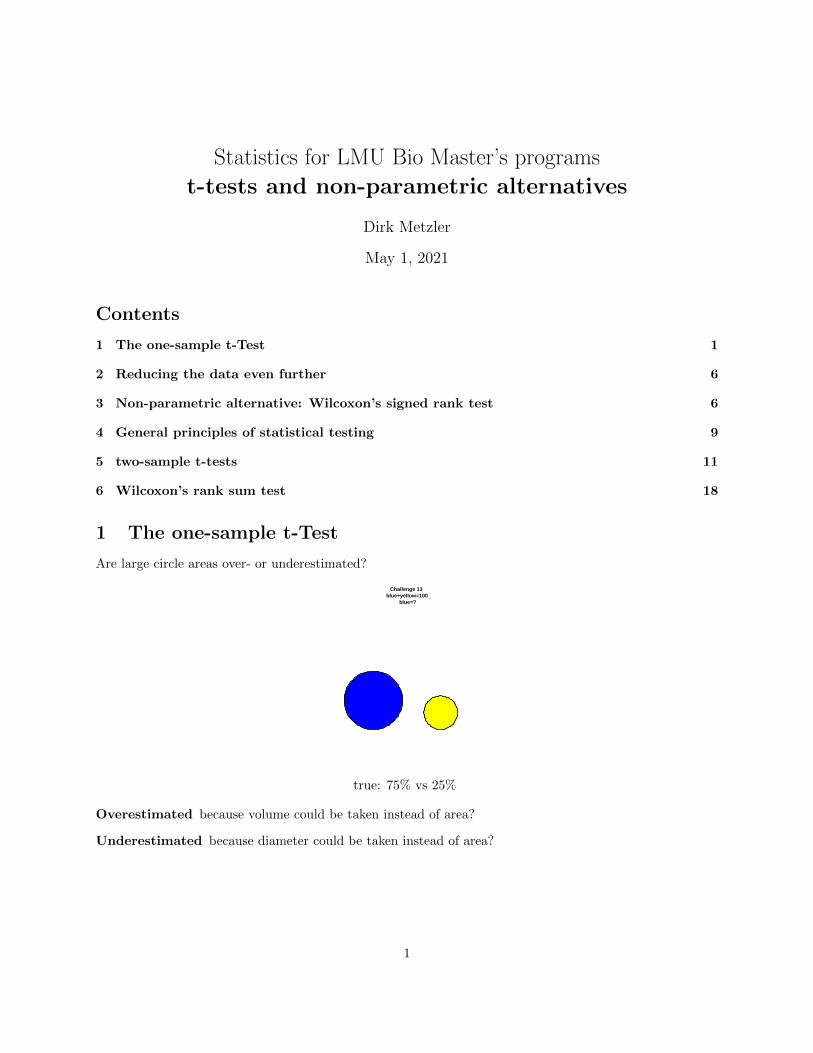
1 The one-sample t-Test
Are large circle areas over- or underestimated?
Challenge 13 blue+yellow=100
blue=?
true: 75% vs 25%
Overestimated because volume could be taken instead of area?
Underestimated because diameter could be taken instead of area?
1

Blue area for plot 13 (circles) estimated by n=24 students (in 2019)
Estimated
Fre
quen
cy
20 30 40 50 60 70 80
01
23
45
6
truemean estimatemean +/− SEM
Null hypothesis: estimation X is unbiased. That is, the mean of the estimated values is
µ := EX = 75
.
Let x1, . . . , xn be the observed values.|x− µ| = |63.6− 75| = 11.4 is 4.37 standard errors (sx/
√n).
t :=x− µsx/√n
= 4.37
The t value is the test statistic in Student’s (that is, Gosset’s) one-sample t-test.If the null hypothesis is true, what is the distribution of t?Assume
X ∼ N (µ, σ2).
⇒ X ∼ N (µ, σ2/n)
⇒ X − µ ∼ N (0, σ2/n)
⇒ X − µσ/√n∼ N (0, 1)
But σ is replaced by s in t, which adds some variation.
General Rule 1. If X1, . . . , Xn are independently drawn from a normal distributed with mean µ and
s2 =1
n− 1
n∑i=1
(Xi −X)2,
then
t =X − µs/√n
is t-distributed with n− 1 degrees of freedom (df).
The t-distribution is also called Student-distribution since Gosset published it using this synonym.
2
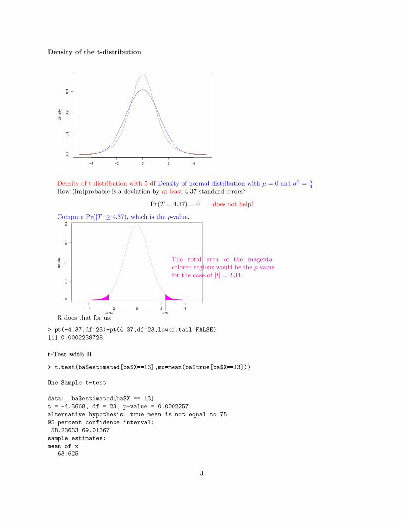
Density of the t-distribution
−4 −2 0 2 4
0.0
0.1
0.2
0.3
dens
ity
Density of t-distribution with 5 df Density of normal distribution with µ = 0 and σ2 = 53
How (im)probable is a deviation by at least 4.37 standard errors?
Pr(T = 4.37) = 0 does not help!
Compute Pr(|T | ≥ 4.37), which is the p-value.
2.34−2.34
−4 −2 0 2 4
0.0
0.1
0.2
0.3
0.4
de
nsity The total area of the magenta-
colored regions would be the p-valuefor the case of |t| = 2.34.
R does that for us:
> pt(-4.37,df=23)+pt(4.37,df=23,lower.tail=FALSE)
[1] 0.0002238728
t-Test with R
> t.test(ba$estimated[ba$X==13],mu=mean(ba$true[ba$X==13]))
One Sample t-test
data: ba$estimated[ba$X == 13]
t = -4.3668, df = 23, p-value = 0.0002257
alternative hypothesis: true mean is not equal to 75
95 percent confidence interval:
58.23633 69.01367
sample estimates:
mean of x
63.625
3
We note:p− value = 0.0002257
i.e.: If the Null hypothesis “just random”, in our case µ = 75, holds, any deviation like the observed oneor even more is very improbable.
If we always reject the null hypothesis if and only if the p-value is below a level of significance of 0.05,then we can say following holds:
If the null hypothesis holds, then the probability that we reject it, is only 0.05.
●
●
● ●
●
●
●
●
●
●
●
●
●
●
●
●
● ●
● ●
●
●
●
●
−2 −1 0 1 2
3040
5060
7080
Normal Q−Q Plot
Theoretical Quantiles
Sam
ple
Qua
ntile
s
Why normal q-q-plot should roughly show a straigth line.
If X ∼ N (µ, σ2), then X−µσ ∼ N (0, 1).
⇒Pr
(X − µσ
< q
)= Pr(X < σ · q + µ)
This means that if q is the p-quantile of N (0, 1), then σ · q + µ is the p-quantile of X.With exact quantiles of N
(µ = 1, σ2 = 0.52
):
●
●●
●● ● ● ● ●●●●●●●●●●●●●●●●●●●●●●●●●
●●●●●●●●
●●●●●●●●
●●●●●●●●
●●●●●●●●
●●●●●●●●●●●●●●●●●●●●●●●●●● ● ● ● ●
●●
●
●
−2 −1 0 1 2
0.0
0.5
1.0
1.5
2.0
qnorm(1:100/100)
qnor
m(1
:100
/100
, mea
n =
1, s
d =
0.5
)
4

Blue area for plot 13 (circles) estimated by n=24 students (in 2019)
Estimated
Fre
quen
cy
20 30 40 50 60 70 80
01
23
45
6
Estimated blue area for plot 13 (circles)
Estimated
Fre
quen
cy
20 30 40 50 60 70 80
01
23
45
6
> t.test(ba$estimated[ba$X==13 & ba$estimated>50],
mu=mean(ba$true[ba$X==13]))
One Sample t-test
data: ba$estimated[ba$X == 13 & ba$estimated > 50]
t = -5.8431, df = 21, p-value = 8.443e-06
alternative hypothesis: true mean is not equal to 75
95 percent confidence interval:
64.02948 69.78870
sample estimates:
mean of x
66.90909
Blue area for plot 13 (circles) estimated by n=24 students (in 2019)
Estimated
Fre
quen
cy
20 30 40 50 60 70 80
01
23
45
6
truemean estimatemean +/− SEM
Estimated blue area for plot 13 (circles)
Estimated
Fre
quen
cy
20 30 40 50 60 70 80
01
23
45
6
truemean estimatemean +/− SEM
But is it really well justfied to remove outliers?
5

Perhaps rather not.
In any case the decision must be documented and reasoned.
2 Reducing the data even further
For our example data we can also try just using the following information:
n = 22 students did not give the correct value of 75
k = 20 of them underestimated the blue area
Null hypothesis is now: overestimation and underestimation have the same probability.As always wefurther assume independence among the estimations. Thus, k is a realization of K ∼ bin(n, 1/2).
0 1 2 3 4 5 6 7 8 9 10 11 12 13 14 15 16 17 18 19 20 21 22
binomial distribution probabilities
0.00
0.05
0.10
0.15
With two-sided testing, the p-value is the sum of all probabilities that are smaller or equal to Pr(K = k).
For p = 1/2 the binomial distribution is symmetric, such that the p-value is
Pr(K ≤ n− k) + Pr(K ≥ k) = Pr(K ≤ 2) + Pr(K ≥ 20) ≈ 0.00012.
> (s <- dbinom(0:n,n,0.5)<=dbinom(k,n,0.5))[1] TRUE TRUE TRUE FALSE FALSE FALSE FALSE FALSE FALSE FALSE FALSE FALSE
[13] FALSE FALSE FALSE FALSE FALSE FALSE FALSE FALSE TRUE TRUE TRUE> sum(dbinom(0:n,n,0.5)[s])[1] 0.0001211166
3 Non-parametric alternative: Wilcoxon’s signed rank test
Wilcoxon’s signed rank testsigned rank: take rank of absolute value, equipped with sign of original value
example:values: −2.6 −2.5 −2.3 −1.3 −0.6 1.6 2.2 6.1absolute values: 2.6 2.5 2.3 1.3 0.6 1.6 2.2 6.1ranks: 7 6 5 2 1 3 4 8signed ranks: −7 −6 −5 −2 −1 3 4 8
Test statistic: V = 3 + 4 + 8 = 15 (sum of positive ranks)
> wilcox.test(c(-2.6,-2.5,-2.3,-1.3,-0.6,1.6,2.2,6.1))
Wilcoxon signed rank test
6

data: c(-2.6, -2.5, -2.3, -1.3, -0.6, 1.6, 2.2, 6.1)
V = 15, p-value = 0.7422
alternative hypothesis: true location is not equal to 0
How many combinations of ranks lead to a certain value of V ?
−1− 2− 3− 4− 5− 6− 7− 8 = −36 V = 0
+1 −2− 3− 4− 5− 6− 7− 8 = −34 V = 1
−1 +2 −3− 4− 5− 6− 7− 8 = −32 V = 2
−1− 2 +3 −4− 5− 6− 7− 8 = −30 V = 3
+1 + 2 −3− 4− 5− 6− 7− 8 = −30 V = 1 + 2 = 3...
......
−1+2 + 3 + 4 + 5 + 6 + 7 + 8 = 34 V = 2 + 3 + · · ·+ 8 = 35
1 + 2 + 3 + 4 + 5 + 6 + 7 + 8 = 36 V = 1 + 2 + · · ·+ 8 = 36
The null hypothesis implies that for each rank the sign is purely random.Thus, each line above has aprobability of 1/2n.There are e.g. two ways of getting a V = 3 and two of getting V = 33.
Pr(V = 3) = Pr(V = 33) =2
28= 0.0078
Numbers of possibilities for each possible value of V for n = 8
0 1 2 3 4 5 6 7 8 9 10 11 12 13 14 15 16 17 18 19 20 21 22 23 24 25 26 27 28 29 30 31 32 33 34 35 36
02
46
810
1214
Probabilities under H0 of possible values of V for n = 8
7

0 1 2 3 4 5 6 7 8 9 10 11 12 13 14 15 16 17 18 19 20 21 22 23 24 25 26 27 28 29 30 31 32 33 34 35 36
0.00
0.01
0.02
0.03
0.04
0.05
example
values: −2.6 −2.5 −2.3 −1.3 −0.6 −0.2 0.1 0.4absolute values: 2.6 2.5 2.3 1.3 0.6 0.2 0.1 0.4ranks: 8 7 6 5 4 2 1 3signed ranks: −8 −7 −6 −5 −4 −2 1 3
p-value for V = 4 (with n = 8):
Pr(V ∈ {0, 1, 2, 3, 4, 32, 33, 34, 35, 36}) =1 + 1 + 1 + 2 + 2 + 2 + 2 + 1 + 1 + 1
28= 0.054
Wilcoxon’s signed rank test
> wilcox.test(c(-2.6,-2.5,-2.3,-1.3,-0.6,-0.2,0.1,0.5))
Wilcoxon signed rank test
data: c(-2.6, -2.5, -2.3, -1.3, -0.6, -0.2, 0.1, 0.5)
V = 4, p-value = 0.05469
alternative hypothesis: true location is not equal to 0
Wilcoxon’s signed rank test
> wilcox.test(ba$estimated[ba$X==13],
mu=mean(ba$true[ba$X==13]))
Wilcoxon signed rank test with continuity correction
data: ba$estimated[ba$X == 13]
V = 6, p-value = 8.779e-05
alternative hypothesis: true location is not equal to 75
Warnmeldungen:
1: In wilcox.test.default(ba$estimated[ba$X == 13], mu = mean(ba$true[ba$X == :
cannot compute exact p value due to bindings
2: In wilcox.test.default(ba$estimated[ba$X == 13], mu = mean(ba$true[ba$X == :
cannot compute exact p value due to bindings
8

4 General principles of statistical testing
• We want to argue that some deviation in the data is not just random.
• To this end we first specify a null hypothesis H0, i.e. we define, what “just random” means.
• Then we try to show: If H0 is true, then a deviation that is at least at large as the observed one, isvery improbable.
• If we can do this, we reject H0.
• How we measure deviation, must be clear before we see the data.
Statistical Testing: Important terms
null hypothesis H0 : says that what we want to substantiate is not true and anything that looks likeevidence in the data is just random. We try to reject H0.
significance level α : If H0 is true, the probability to falsely reject it, must be ≤ α (often α = 0.05).
test statistic : measures how far the data deviates from what H0 predicts into the direction of our alter-native hypothesis.
p value : Probability that, if H0 is true, a dataset leads to a test statistic value that is as least as extremeas the observed one.
• We reject the null hypothesis H0 if the p value is smaller than α.
• Thus, if H0 is true, the probability to (falsely) reject it is α (not the p value).
• This entails that a researcher who performs many tests with α = 0.05 on complete random data (i.e.where H0 is always true), will falsely reject H0 in 5% of the tests.
• Therefore it is a severe violation of academic soundness to perform tests until one shows significance,and to publish only the latter.
Testing two-sided or one-sided?
We observe a value of x that is much larger than theH0 expectation value µ.
−4 −2 0 2 4
0.0
0.1
0.2
0.3
0.4
density
2.5%2.5%
p-value=PrH0(|X − µ| ≥ |x− µ|)
−4 −2 0 2 4
0.0
0.1
0.2
0.3
0.4
density
5.0%p-value=PrH0
(X ≥ x)
9
The pure teachings of statistical testing
• Specify a null hypothesis H0, e.g. µ = 0.
• Specify level of significance α, e.g. α = 0.05.
• Specify an event A such thatPrH0
(A) = α
(or at least PrH0(A) ≤ α). e.g. A = {X > q} or A = {|X − µ| > r} in general: A = {p-value ≤ α}
• AND AFTER THAT: Look at the data and check if if A occurs.
• Then, the probability that H0 is rejected in the case that H0 is actually true (“Type I error”) is justα.
Violations against the pure teachings
“The two-sided test gave me a p-value of 0.06. Therefore, I tested one-sidedand this worked out nicely.”
is as bad as:
“At first glance I saw that x is larger than µH0. So, I immediately applied
the one-sided test.”
ImportantThe decision between one-sided and two-sided must not depend on the concrete data that are used in thetest. More generally: If A is the event that will lead to the rejection of H0, (if it occurs) then A must bedefined without being influenced by the data that is used for testing.
This means: Use separate data sets for exploratory data analysis and for testing.In some fields these rules are followed quite strictly, e.g. testing new pharmaceuticals for accreditation.In some other fields the practical approach is more common: Just inform the reader about the p-values
of different null-hypotheses.
Severe violations against scientific standards
HARKing: Hypothesize After Results Known
p-hacking: try out different tests and different preprocessing methods until you obtain significance
If H0 is rejected on the 5%-level, which of the following statements is true?
• The null hypothesis is wrong.
• H0 is wrong with a probability of 95%.
• If H0 is true, you will see such an extreme event only in 5% of the data sets. X
If the test did not reject H0, which of the following statements are true?
10
• We have to reject the alternative H1.
• H0 is true
• H0 is probably true.
• It is safe to assume that H0 was true.
• Even if H0 is true, it is not so unlikely that our test statistic takes a value that is as extreme as theone we observed.X
• With this respect, H0 is compatible with the data.X
Some of what you should be able to explain
• Structure of t-statistic and df for one-sample t-test
• what is a qqnorm plot and how can it be used to check normality
• Rationale of Wilcoxon’s signed rank test and how to compute its test statistic
• principles of statistical testing and exact meaning of
– p-value
– significance level α
– null hypothesis
• how to report significance and non-significance
5 two-sample t-tests
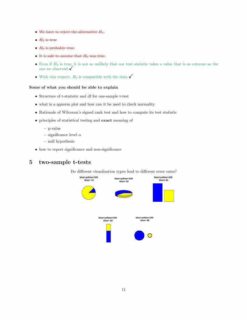
Do different visualization types lead to different error rates?
blue+yellow=100 blue= 12
blue+yellow=100 blue= 62
blue+yellow=100 blue= 61
blue+yellow=100 blue= 62
blue+yellow=100 blue= 86
11
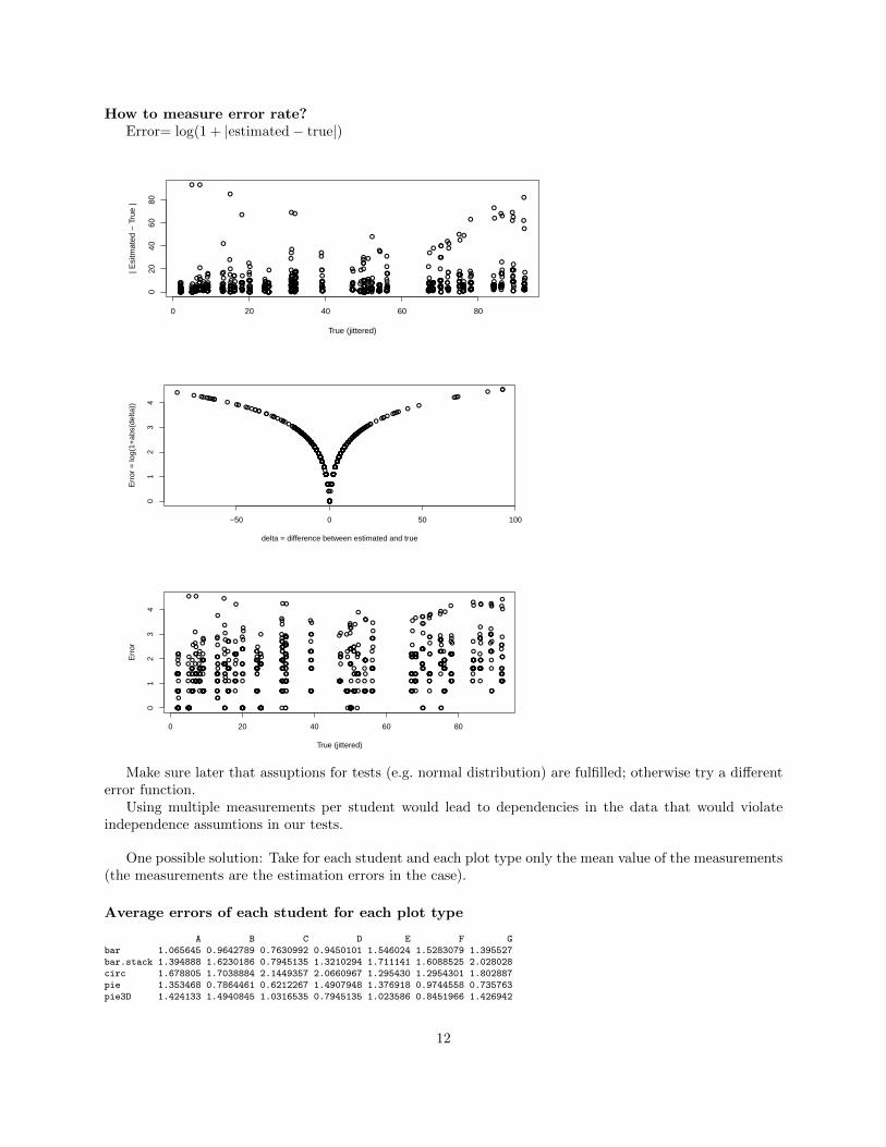
How to measure error rate?Error= log(1 + |estimated− true|)
●
●
●● ●● ● ●●
●●
●●
● ● ●
● ●● ● ●
●
●●●●
●
●
●●●●●
● ●
●
●
●
●●
●
●
●● ●● ● ●●●●
●
●● ● ●
● ●●●
●●
●●●●
●
● ●●
●●
●●
● ●●
●
●● ● ●●● ●● ● ●●● ●●
●
●●
●
● ●● ●
●
● ●● ●●
●
●
●
● ●●● ● ● ●●●
●● ● ●●●
●● ● ●●
● ●●
●
●● ●
● ●● ●
●
● ●● ●
● ●
●
●
● ●●● ● ●
●
●● ●● ●●●
● ●● ● ●●●
●●●
● ● ●●
●
●
● ●
●
●●
●
● ●●●● ●
●
● ● ●●
●
● ●
● ●
●
●●
●
● ● ●●● ●● ●●
● ●● ●●
●●
● ●● ●●
●
● ●●
●●
● ● ● ●●● ●● ● ●●
● ●●
●●
●●
●
●
●●●
●
●
●
●
● ●
● ●
●●●
●
●
●● ●
●
● ● ● ●●●
●●
●
●
●● ●
● ● ●●●
●
●●
● ● ●● ●● ●
●
● ●● ●● ●●
●●●●● ● ● ●●● ●● ● ●●
● ●●
●
●
●
●
●● ●● ●
●
●
●
●
●
●
●
●● ●
● ●
●
●●●
●
●● ●
●
●
●
●●
● ●●
● ●●
●●
●●
●
●
●●●
●
●
●
●
● ●
● ●
●●●
●
●
●● ●
●
● ● ● ●●●
●●
●
●
●●●●
●
●●
●●
●●
● ● ●●
●
● ● ●●●●
●●
●● ●
●●●● ●
● ●●● ●
●
●
●
●● ●
●
● ●
●●
●●
●
● ●
●
●
●
●●
●
●
●
●
●●
●
●
●●
●
● ●
●
●
●
●
●
●
●
●
●
●●
●
●●
●●●
●
● ●
●
● ●●●
●
●●
● ●●
●
●●● ●●●
●
●
●
●● ●● ●
●
●●
●
●●
●
●●
●
●
●
●
●●
● ●●
●
●
● ●●
●
●
●
●
●
● ●
●
● ●
●
●
●●
●●
●●●● ●
●
●
●
●
●
●
●
●●
●
●
● ●● ●
●●
●
●
●
●
●
●
●●
●
●
●
●
● ●●
●
●
●
●●●
● ●● ● ●●● ●●
●
●●
●
● ●●●
●
● ●● ●●
●
●
●
● ●●●● ●
●●● ●
● ● ●●● ●●
●
●
●
●
●●
●
● ● ●
●
●● ●
●●
●
● ●
●
●●
●
● ●●
● ● ● ●●● ●
●
●
●●● ●● ● ●●
●
●
●
●
●● ●
● ●●●
●
●●
●
●
●
●
●
●
●
●
●● ●●
●●●
●
●
●
●
●● ●● ● ●●
● ●●
●●●
●
●● ● ●
●●
●
●
●
●
●●● ●
●●
●
●●●● ●● ● ●●
● ●●
●
●
●● ●●●
● ● ●●
●● ●
●●
●●●●
●
●●● ●●●
●●
●●●
●
●
● ●●● ●
●●
●
●● ●
●
●
●
● ●
●●● ● ●●
●●
●
●
●
●●
●
●
●
● ●●
●●●
●
●
● ●●● ●● ● ●●●
●
● ●
● ● ●
●
●
● ● ●
●●
● ●●
●
●
●
●
●●●
●
● ●●● ●●
●
●●●●●
●
●●● ●●
●
●
●
●
●
●
●● ●
●
●●
●
● ●●
●
●
●
●
●
●
●●●
●
●●
●
●
●● ●● ●
●
●●
●
●●
● ●●
●
●
● ● ●
●
●●
●●
●
● ●● ●
●●
●
●
●●●
●●
0 20 40 60 80
020
4060
80
True (jittered)
| Esi
tmat
ed −
Tru
e |
●
●
●
●
●
●
●
●
●
●
●
●
●
●
●
●
●
●
●
●
●
●
●●
●●
●
●
●
●
●●
●
●●
●
●
●
●
●
●
●
●
●
●
●●
●
●
●
●
●
●●
●●
●
●
●
●
●●
●●
●
●
●
●
●
●
●
●
●
●
●
●●
●
●
●●
●
●
●
●
●
●●
●
●
●
●
●
●
●
●
●
●
●
●
●
●
●●●
●
●
●
●
●●
●
●
●
●
●●
●
●
●●
●
●
●
●
●
●
●
●
●●
●
●
●
● ●
●
●
●●
●
●●
●●
●●
●
●
●
●●
●
●
●
●
●
●
●
●●
●
●
●●●●
●
●
●
●
●
●
●
●
●
●
●
●
●●
●
●●
●
●●
●
●
●
●
●
●
●
●
●
●
●●
●●
●
●
●
●
●
●
●
●
●●
●
●
●
●●●
●
●
●
●
●
●
● ●
●
●
●
●
●
●●
●●●●●●
●
●●
●
●
●
●
●
●
●
●
●
●
●
●●
●
●
●
●
●
●
●
●●
●
●
●
●
●
●
●●
●
●●
●●
●
●
●
●
●
●
●
●●
●●
●
●
●
●
●
●
●
● ●
●
●
●
●
●
●●●●
●
●
●
●
●
●●
●
●●
●●
●
●
●●
●
●
●●
●
●
●
●
●
●
●
●
●
●
●
●
●
●
●
●
●
●●●
●●
●
●
●
●
●
●
●●
●
●
●
●
●
●
●
●
●
●
●
●
●
●
●
●
●
●●
●
●
●
●
●
●
●
●●
●
●
●
●
●
●
●●
●
●●
●●
●
●
●
●
●
●
●
●
●●
●
●
●
●
●
●
●
●
●
●
●
●
●●
●●
●●
●
●
●
●
●
●
●
●
●●
●●
●
●
●
●
●
●
●
●●
●
●●
●●
●●
●
●
●
●
●
●
●
●
●
●
●
●
●
●
●
●
●●
●
●
●
●
●
●
●
●
●
●
●
●
●
●
●
●
●
●
●
●
●
●
●
●
●
●
●
●
●
●
●
●●
●
●
●
●
●
●
●
●
●
●
●
●
●
●
●●
●
●
●
●
●
●
●
●
●
●
●
●
●
●●
●
●
●
●
●
●
●
●
●
●
●
●
●
●
●
●
●●
●
●
●
●
●
●
●
●
●
●
●
●
●
●
●
●
●
●
● ●
●
●
●
●●
●
●
●
●
●
●
●
●
●
● ●
●
●
●
●
●●
●
●●
●
●
●
●
●
●●
●
●
●
●
●
●
●
●
●
●
●●
●
●
●
●
●
●
●
●
●
●
●
●●
●●
●
●
●
●
●●
●●
●
●
●
●
●
●
●
●
●
●
●
●
●
●●
●
●
●●
●
●
●
●●
●
●●
●
●
●
●
●●
●
●●
●●
●
●
●
●
●●
●
●
●
●
●
●
●
●
●
● ●
●
●
●
●
●
●
●
●
●
●
●
●
●
●
●
●
●
●
●
●
●
●
●
●
●
●
●
●
●
●●
●
●
●●
●
●●
●
●
●
●
●
●
●
●
●
●
●
●
●
●
●
●
●●
●
●
●
●●● ●
●
●
●
●●
●
●
●
●
●
●
●
●
●
●
●
●
●
●●
●
●
●●
●
●
●
●
●
●
●
●
●
●
●
●●
●
●
●
●
●
●
●
●
●
●
●
●
●●
●
●
●
●●
●
●
●●
●●
●●
●
●
●
●
●
●
●
●
●●
●
●●
●
●
●
●
●
●
●
●
●
●●
●
●
●
●
●
●
●●
●
●
●
●
●
●
●
●●●
●
●
●
●
●●
●
●
●●
●
●●
●
●
●●
●
●●
●
●
●
●
●
●
●
●
●●
●
●
●
●●
●
●●
●
●
●
●
●
●
●
●
●
●
●
●
●
●
●
●
●
●
●
●
●
●
●
●
●
●
●
●
●
●●
●
●
●
●●
●
●
●
●
●●
●
●
●
●●
●
●
●
●
●
●
●
●
●
−50 0 50 100
01
23
4
delta = difference between estimated and true
Err
or =
log(
1+ab
s(de
lta))
●
●
●
●
●
●
●
●
●
●
●
●
●
●
●
●
●
●
●
●
●
●
●●
●●
●
●
●
●
●●
●
● ●
●
●
●
●
●
●
●
●
●
●
● ●
●
●
●
●
●
●●
● ●
●
●
●
●
●●
●●
●
●
●
●
●
●
●
●
●
●
●
●●
●
●
● ●
●
●
●
●
●
● ●
●
●
●
●
●
●
●
●
●
●
●
●
●
●
●● ●
●
●
●
●
●●
●
●
●
●
●●
●
●
● ●
●
●
●
●
●
●
●
●
●●
●
●
●
● ●
●
●
● ●
●
● ●
●●
●●
●
●
●
●●
●
●
●
●
●
●
●
● ●
●
●
●●● ●
●
●
●
●
●
●
●
●
●
●
●
●
●●
●
●●
●
● ●
●
●
●
●
●
●
●
●
●
●
●●
● ●
●
●
●
●
●
●
●
●
●●
●
●
●
● ●●
●
●
●
●
●
●
● ●
●
●
●
●
●
●●
● ● ● ●●●
●
● ●
●
●
●
●
●
●
●
●
●
●
●
●●
●
●
●
●
●
●
●
● ●
●
●
●
●
●
●
●●
●
● ●
● ●
●
●
●
●
●
●
●
●●
● ●
●
●
●
●
●
●
●
● ●
●
●
●
●
●
● ●● ●
●
●
●
●
●
●●
●
● ●
●●
●
●
● ●
●
●
●●
●
●
●
●
●
●
●
●
●
●
●
●
●
●
●
●
●
●● ●
●●
●
●
●
●
●
●
●●
●
●
●
●
●
●
●
●
●
●
●
●
●
●
●
●
●
●●
●
●
●
●
●
●
●
● ●
●
●
●
●
●
●
●●
●
● ●
● ●
●
●
●
●
●
●
●
●
●●
●
●
●
●
●
●
●
●
●
●
●
●
●●
●●
●●
●
●
●
●
●
●
●
●
● ●
● ●
●
●
●
●
●
●
●
●●
●
● ●
●●
●●
●
●
●
●
●
●
●
●
●
●
●
●
●
●
●
●
●●
●
●
●
●
●
●
●
●
●
●
●
●
●
●
●
●
●
●
●
●
●
●
●
●
●
●
●
●
●
●
●
● ●
●
●
●
●
●
●
●
●
●
●
●
●
●
●
● ●
●
●
●
●
●
●
●
●
●
●
●
●
●
● ●
●
●
●
●
●
●
●
●
●
●
●
●
●
●
●
●
● ●
●
●
●
●
●
●
●
●
●
●
●
●
●
●
●
●
●
●
●●
●
●
●
●●
●
●
●
●
●
●
●
●
●
●●
●
●
●
●
● ●
●
●●
●
●
●
●
●
●●
●
●
●
●
●
●
●
●
●
●
●●
●
●
●
●
●
●
●
●
●
●
●
●●
●●
●
●
●
●
●●
● ●
●
●
●
●
●
●
●
●
●
●
●
●
●
● ●
●
●
● ●
●
●
●
● ●
●
●●
●
●
●
●
● ●
●
●●
●●
●
●
●
●
●●
●
●
●
●
●
●
●
●
●
● ●
●
●
●
●
●
●
●
●
●
●
●
●
●
●
●
●
●
●
●
●
●
●
●
●
●
●
●
●
●
● ●
●
●
●●
●
●●
●
●
●
●
●
●
●
●
●
●
●
●
●
●
●
●
●●
●
●
●
●●
●●
●
●
●
●●
●
●
●
●
●
●
●
●
●
●
●
●
●
●●
●
●
●●
●
●
●
●
●
●
●
●
●
●
●
●●
●
●
●
●
●
●
●
●
●
●
●
●
●●
●
●
●
●●
●
●
●●
●●
●●
●
●
●
●
●
●
●
●
● ●
●
●●
●
●
●
●
●
●
●
●
●
●●
●
●
●
●
●
●
● ●
●
●
●
●
●
●
●
● ●●
●
●
●
●
●●
●
●
●●
●
●●
●
●
●●
●
●●
●
●
●
●
●
●
●
●
●●
●
●
●
●●
●
●●
●
●
●
●
●
●
●
●
●
●
●
●
●
●
●
●
●
●
●
●
●
●
●
●
●
●
●
●
●
●●
●
●
●
●●
●
●
●
●
●●
●
●
●
● ●
●
●
●
●
●
●
●
●
●
0 20 40 60 80
01
23
4
True (jittered)
Err
or
Make sure later that assuptions for tests (e.g. normal distribution) are fulfilled; otherwise try a differenterror function.
Using multiple measurements per student would lead to dependencies in the data that would violateindependence assumtions in our tests.
One possible solution: Take for each student and each plot type only the mean value of the measurements(the measurements are the estimation errors in the case).
Average errors of each student for each plot type
A B C D E F Gbar 1.065645 0.9642789 0.7630992 0.9450101 1.546024 1.5283079 1.395527bar.stack 1.394888 1.6230186 0.7945135 1.3210294 1.711141 1.6088525 2.028028circ 1.678805 1.7038884 2.1449357 2.0660967 1.295430 1.2954301 1.802887pie 1.353468 0.7864461 0.6212267 1.4907948 1.376918 0.9744558 0.735763pie3D 1.424133 1.4940845 1.0316535 0.7945135 1.023586 0.8451966 1.426942
12
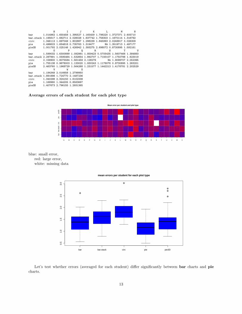
H I J K L M Nbar 1.014962 1.655458 1.395527 1.165459 1.798220 1.3727371 2.605710bar.stack 1.195617 1.682711 2.028028 1.637742 1.758303 1.1670114 1.316792circ 1.346113 1.697049 1.802887 1.298239 1.845993 2.0249917 3.026309pie 0.498623 1.654818 0.735763 1.319477 NA 1.3519713 1.497177pie3D 1.001792 2.025146 1.426942 1.393275 2.698072 0.8730895 1.592161
O P Q R S T Ubar 1.599032 1.6300899 1.092981 1.859423 0.5705435 1.5607468 1.384883bar.stack 2.297891 1.0595464 1.532854 1.892707 1.7193107 1.1750788 1.623019circ 2.158900 1.8075584 1.561459 2.128278 NA 1.9099707 2.052395pie 1.755138 0.9678003 1.133020 1.930243 1.1178076 0.8730895 1.263201pie3D 2.463760 1.1968729 1.564268 1.231577 1.1442213 1.4176781 2.202529
V W Xbar 1.194348 2.016658 1.2799950bar.stack 1.891898 1.724770 2.1487236circ 1.340298 2.324150 1.6102338pie 1.168980 1.344205 0.8583667pie3D 1.407673 2.796155 1.2931365
Average errors of each student for each plot type
Mean error per student and plot type
bar
bar.s
tack
circ
pie
pie3
D
A B C D E F G H I J K L M N O P Q R S T U V W X
blue: small error,red: large error,white: missing data
●
●
●
●
●
bar bar.stack circ pie pie3D
0.5
1.0
1.5
2.0
2.5
3.0
mean errors per student for each plot type
Let’s test whether errors (averaged for each student) differ significantly between bar charts and piecharts.
13

Bar charts, n=24
Average error over 8 plots
Fre
quen
cy0.0 0.5 1.0 1.5 2.0 2.5 3.0
01
23
45
Pie charts, n=23
Average error over 8 plots
Fre
quen
cy
0.0 0.5 1.0 1.5 2.0 2.5 3.0
02
46
●
●
●
●
●●
●
●
●
●
●
●
●
●
●●
●
●
●
●
●
●
●
●
−2 −1 0 1 2
0.5
1.0
1.5
2.0
2.5
Normal Q−Q plot for bar chart errors
Theoretical Quantiles
Sam
ple
Qua
ntile
s
●
●
●
●
●
●
●
●
●
●
●●
●
●
●
●
●
●
●
●
●
●
●
−2 −1 0 1 2
0.6
0.8
1.0
1.2
1.4
1.6
1.8
Normal Q−Q plot for pie chart errors
Theoretical Quantiles
Sam
ple
Qua
ntile
s
> t.test(M["bar",],M["pie",])
Welch Two Sample t-test
data: M["bar", ] and M["pie", ]
t = 1.9106, df = 44.466, p-value = 0.06252
alternative hypothesis: true difference in means is not equal to 0
95 percent confidence interval:
-0.01233732 0.46486341
sample estimates:
mean of x mean of y
1.391861 1.165598
Theorem 1 (Welch’s t-test). Suppose that X1, . . . , Xn and Y1, . . . , Ym are independent and normally dis-tributed random variables with EXi = EYj and potentially different variances VarXi = σ2
X and VarYi = σ2Y .
Let s2X and s2Y be the sample variances. The statistic
t =X − Y√s2Xn +
s2Ym
14

approximately follows a t distribution with (s2Xn +
s2Ym
)2s4X
n2·(n−1) +s4Y
m2·(m−1)
degrees of freedom.
> t.test(M["bar",],M["pie",],var.equal=TRUE)
Two Sample t-test
data: M["bar", ] and M["pie", ]
t = 1.9043, df = 45, p-value = 0.06328
alternative hypothesis: true difference in means is not equal to 0
95 percent confidence interval:
-0.01305144 0.46557752
sample estimates:
mean of x mean of y
1.391861 1.165598
Theorem 2 (Student’s two-sample t-test, unpaired with equal variances). Suppose that X1, . . . , Xn andY1, . . . , Ym are independent and normally distributed random variables with the same mean µ and the samevariance σ2. Define the pooled sample variance to be
s2p =(n− 1) · s2X + (m− 1) · s2Y
m+ n− 2.
The statistic
t =X − Y
sp ·√
1n + 1
m
follows a t distribution with n+m− 2 degrees of freedom.
Have we missed some relevant information?Maybe there was variation in error among the students.
We can remove this variation by paired testing, that is, apply one-sample t-test to differences in errorper student.
0.5 1.0 1.5 2.0 2.5
bar
pie
average error for each student
●
●
●
●●
●
●
●
●
●
● ●●
●
●
●
●
●
●
●●
●
●
0.0 0.5 1.0 1.5 2.0 2.5 3.0
0.0
0.5
1.0
1.5
2.0
2.5
3.0
Mean errors for bar charts
Mea
n er
rors
for
pie
char
ts
Difference error bar − pie
Fre
quen
cy
−0.5 0.0 0.5 1.0
01
23
45
67
> t.test(M["bar",],M["pie",],paired=TRUE)
Paired t-test
data: M["bar", ] and M["pie", ]
t = 2.3331, df = 22, p-value = 0.02918
15

alternative hypothesis: true difference in means is not equal to 0
95 percent confidence interval:
0.02317965 0.39401089
sample estimates:
mean of the differences
0.2085953
●
●●
●
●
●
●
●
●
●
●
●
●
●
●
●●
●
●
●
●
●
●
−2 −1 0 1 2
−0.
50.
00.
51.
0
Normal Q−Q plot for difference between bar and pie chart errors
Theoretical Quantiles
Sam
ple
Qua
ntile
s
Note: what we did here looks like we tried out several tests until a test indicated significance.
This would be a severe violation of the principles of statistical testing andof good scientific practice!
The various tests were applied above only to show the differences for teaching purposes. (So do as I say,not as I apparently did.)
Correct: before looking at the data, anticipate that between-student variationis possible and decide to apply paired t-test.
What is the conclusion from our test?Let’s assume the 24 test persons were chosen randomly among all LMU biology students (which was
actually not the case).
Can we say
“LMU biology students could guess fractions significantly better from pie charts (of thiskind) than from bar charts (of this kind).”
or can we only say
“LMU biology students could guess fractions significantly better from these 8 pie chartsthan from these 8 bar charts.”
???
• The true value of each plot may influence the error distribution.
16

• In fact, the pie and bar charts were randomly generated from a class of charts for which they arerepresentative
– blue and yellow colour
– blue area is a purely randonm value from {1, 2, . . . , 99}.
• Thus, each single plot had the same chance to have a difficult or an easy true value.
• But the values used for the t-test were not the independent observations of each plot but averages over8 plots of each type.
• Thus, each of the eight plots was used in all 23 (or 24) values, and the t-test (standard errors indenominator of t) could not account for the variation between plots.
This implies that the results could be representative for LMU biology students (if the testpersons had been sampled randomly) but not for a class of pie/bar plots.
How can we apply the t-test to independent values for each plot?
Average for each plot the errors from all students:pie.err 0.24 0.05 1.46 0.94 1.77 1.58 1.98 1.50bar.err 1.07 1.44 1.96 0.54 1.49 1.54 1.65 1.44
(for one of the pie charts we averaged over only 23 student errors as one was NA.)
0.0 0.5 1.0 1.5 2.0
pie.
err
bar.e
rr
●● ●● ●● ●●
● ● ●● ●● ●●
> t.test(pie.err,bar.err)
Welch Two Sample t-test
data: pie.err and bar.err
t = -0.69367, df = 11.407, p-value = 0.5018
alternative hypothesis: true difference in means is not equal to 0
95 percent confidence interval:
-0.8464499 0.4394227
sample estimates:
mean of x mean of y
1.188347 1.391861
So, if we use the errors values for strip charts and bar charts in a way such that they are representativefor charts of their class, the differences in error values are not significant any more.
But were the students representative for other students in this analysis?
17

No, because we averaged over the students, such that the t-test could not account for variation amongthe students.
Anyway, we could not find significant differences (maybe because of the small number of plots of eachtype?), but even if we had found significant differences, the study design would not allow to draw conclusionsabout other students than the ones involved in the experiment.
How could we draw conclusions about a class of pie charts and bar charts and about a larger populationof persons?
With different tests, e.g. nested anova / mixed-effects models.
or:
With a different study design, e.g. many students, each sees only one bar chart and one pie chart; alwaysnew ones.
6 Wilcoxon’s rank sum test
Wilcoxon’s rank sum test (or equivalently Mann-Whitney U test) is a non-parametric alternative for theunpaired two-sample t-test with equal variances. (But not for Welch’s t-test!)
References
[1] Wilcoxon, F. (1945). Individual comparisons by ranking methods. Biometrics Bulletin 1:8083.
[2] Mann, H. B., Whitney, D. R. (1947). On a test of whether one of two random variables is stochas-tically larger than the other. Annals of Mathematical Statistics 18:5060.
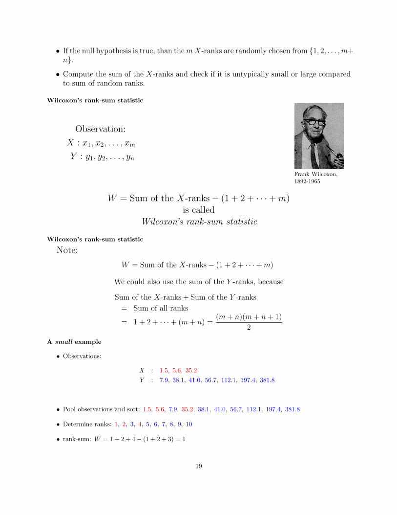
Observations: Two samples
X : x1, x2, . . . , xm
Y : y1, y2, . . . , yn
Test the null hypothesis: that X and Y come from the same population
alternative: X “typically larger” than Y or Y “typically larger” than X
Idea
Observations:
X : x1, x2, . . . , xm
Y : y1, y2, . . . , yn
• Sort all observations by size.
• Determine the ranks of the m X-values among all m+ n observations.
18
• If the null hypothesis is true, than themX-ranks are randomly chosen from {1, 2, . . . ,m+n}.
• Compute the sum of the X-ranks and check if it is untypically small or large comparedto sum of random ranks.
Wilcoxon’s rank-sum statistic
Observation:
X : x1, x2, . . . , xm
Y : y1, y2, . . . , yn
Frank Wilcoxon,1892-1965
W = Sum of the X-ranks− (1 + 2 + · · ·+m)is called
Wilcoxon’s rank-sum statistic
Wilcoxon’s rank-sum statistic
Note:
W = Sum of the X-ranks− (1 + 2 + · · ·+m)
We could also use the sum of the Y -ranks, because
Sum of the X-ranks + Sum of the Y -ranks
= Sum of all ranks
= 1 + 2 + · · ·+ (m+ n) =(m+ n)(m+ n+ 1)
2
A small example
• Observations:
X : 1.5, 5.6, 35.2
Y : 7.9, 38.1, 41.0, 56.7, 112.1, 197.4, 381.8
• Pool observations and sort: 1.5, 5.6, 7.9, 35.2, 38.1, 41.0, 56.7, 112.1, 197.4, 381.8
• Determine ranks: 1, 2, 3, 4, 5, 6, 7, 8, 9, 10
• rank-sum: W = 1 + 2 + 4− (1 + 2 + 3) = 1
19

Significance
Null hypothesis:X-sample and Y -sample were taken from the same distribution
The 3 ranks of the X-sample 1 2 3 4 5 6 7 8 9 10
could just as well have been any 3 ranks 1 2 3 4 5 6 7 8 9 10
There are 10·9·83·2·1 = 120 possibilities.
(In general: (m+n)(m+n−1)···(n+1)m(m−1)···1 ) = (m+n)!
n!m!=
(m+nm
)possibilities)
Distribution or the Wilcoxon statistic (m = 3, n = 7)[1ex]
0 2 4 6 8 10 13 16 19
W
Mög
lichk
eite
n
02
46
810
Under the null hypothesis all rank configurations are equally likely, thus
P(W = w) =number of possibilities with rank-sum statistic w
120
We see in our example: 1.5, 5.6, 7.9, 35.2, 38.1, 41.0, 56.7, 112.1, 197.4, 381.8 W = 1
P(W ≤ 1) + P(W ≥ 20) = P(W = 0) + P(W = 1) + P(W = 20) + P(W = 21) = 1+1+1+1120
·= 0.033
20

Distribution of the Wilcoxon statistic (m = 3, n = 7)[1ex]
0 2 4 6 8 10 13 16 19
W
Wah
rsch
einl
ichk
eit
0.00
0.02
0.04
0.06
0.08
For our example (W = 1):
p-value = P(such an extreme W ) = 4/120 = 0.033
We reject the null hypothesis, that the distributions of X and Y were equal,on the 5%-level.
Wilcoxon test in R with wilcox.test:
> x
[1] 1.5 5.6 35.2
> y
[1] 7.9 38.1 41.0 56.7 112.1 197.4 381.8
> wilcox.test(x,y)
Wilcoxon rank sum test
data: x and y
W = 1, p-value = 0.03333
alternative hypothesis: true location shift is
not equal to 0
IMPORTANT!Can Wilcoxon’s rank sum test replace Welch’s t-test? Not in general, because its null
hypothesis is that the data come from the same distribution, not just that the means areequal. If we want to test whether the means are different but allow the standard deviations tobe different (like in the assumptions of Welch’s t-test), the Wilcoxon test cannot be applied!
21

Some of what you should be able to explain
• Structure of t-statistic and df for
– one-sample t-test
– paired two-sample t-test
– unpaired two-sample t-test
∗ with equal variances
∗ Welch’s t-test
• when and why to use the different t-test variants
• summarizing measurements in a statistic (here: our Error function) that fulfills basic assumptions ofthe test
• summarize data to avoid dependencies; e.g. average over multiple measurements
• Assumptions of Wilcoxon’s rank sum test and when and how to apply it.
see also the topics listed on page 11
22
Top Related