


Languages
Pages
Legal


Statistics and Machine Learning via a ModernOptimization Lens
Dimitris Bertsimas
Operations Research CenterMassachusetts Institute of Technology
June 2015
Bertsimas (MIT) Statistics via Optimization June 2015 1 / 48

Outline
1 Motivation
2 Best Subset SelectionJoint work with Angie King and Rahul Mazumder.
3 Least Median of Squares RegressionJoint work with Rahul Mazumder, Annals of Statistics, 2014
4 An Algorithmic Approach to Linear RegressionJoint work with Angie King.
5 Conclusions
Bertsimas (MIT) Statistics via Optimization June 2015 2 / 48

Motivation
Motivation
Continuous optimization methods have historically played a significantrole in statistics
In the last two decades convex optimization methods have hadincreasing importance: Compressed Sensing, Matrix Completionamong many others
Many problems in statistics and machine learning can naturally beexpressed as Mixed integer optimizations (MIO) problems
MIO in statistics are considered impractical and the correspondingproblems intractable
Heuristics methods are used: Lasso for best subset regression orCART for optimal classification.
Bertsimas (MIT) Statistics via Optimization June 2015 3 / 48

Progress of MIO
Progress of MIO
Speed up between CPLEX 1.2 (1991) and CPLEX 11 (2007): 29,000times
Gurobi 1.0 (2009) comparable to CPLEX 11
Speed up between Gurobi 1.0 and Gurobi 5.5 (2013): 20 times
Total speedup: 580,000 times
A MIO that would have taken 7 years to solve 20 years ago can nowbe solved on the same 20-year-old computer in less than one second.
Hardware speedup: 105.5= 320,000 times
Total Speedup: 200 Billion times!
Bertsimas (MIT) Statistics via Optimization June 2015 4 / 48

Progress of MIO
Research Objectives
Given the dramatically increased power of MIO, is MIO able to solvekey multivariate statistics problems considered intractable a decadeago?
How do MIO solutions compete with state of the art solutions?
Building Regression models is an art. Can we algorithmize theprocess?
What are the implications on teaching statistics?
Bertsimas (MIT) Statistics via Optimization June 2015 5 / 48

Progress of MIO
Problems
Best Subset Regression:
minβ
1
2‖y − Xβ‖22 subject to ‖β‖0 ≤ k
Least Median Regression:
minβ
mediani=1,...,n
|yi − xTi β|
Algorithmic Regression to accomodate Sparsity, Limitingmulticollinearity, Categorical variables, Group sparsity, Nonlineartransformations, Robustness, Statistical significance
Bertsimas (MIT) Statistics via Optimization June 2015 6 / 48

Best Subset Regression
Best Subset Regression
minβ
1
2‖y − Xβ‖22 subject to ‖β‖0 ≤ k
Furnival and Wilson (1974) solve it by implicit enumeration, leapsroutine in R. Cannot scale beyond p = 30.
Lasso proposed in Tibshirani (1996) [13,500 citations] and Chen,Donoho and Saunders (1998) [7100 citations] scale to very largeproblems: via convex quadratic optimization
minβ
12‖y − Xβ‖22 + λ
∑i
|βi |
Under regularity conditions on X, Lasso leads to sparse models andgood predictive performance.
Bertsimas (MIT) Statistics via Optimization June 2015 7 / 48
Best Subset Regression
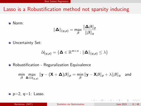
Lasso is a Robustification method not sparsity inducing
Norm:
‖∆‖(q,p) = maxβ
‖∆β‖p‖β‖q
Uncertainty Set:
U(q,p) = {∆ ∈ Rm×n : ‖∆‖(q,p) ≤ λ}
Robustification - Reguralization Equivalence
minβ
max∆∈U(q,p)
‖y − (X + ∆)β‖p = minβ‖y − Xβ‖p + λ‖β‖q and
p=2, q=1: Lasso.
Bertsimas (MIT) Statistics via Optimization June 2015 8 / 48

Best Subset Regression
Our approach
Natural MIO formulation
minβ,z
12‖y − Xβ‖22
subject to |βi | ≤ M · zi , i = 1, . . . , pp∑
i=1zi ≤ k
zi ∈ {0, 1}, i = 1, . . . , p
First Order methods to find good feasible solutions as warm-starts
Enhance MIO by warm-starts and improved formulation
Bertsimas (MIT) Statistics via Optimization June 2015 9 / 48

Best Subset Regression
Parameters
µ := maxi 6=j |〈xi , xj〉|.
µ(m) := max|I|=m maxj /∈I
∑i∈I |〈xj , xi 〉| ≤ mµ
|〈x(1), y〉| ≥ |〈x(2), y〉| . . . ≥ |〈x(p), y〉|
M = min
{1ηk
√∑ki=1 |〈x(i), y〉|2,
1√ηk‖y‖2
}
ηk = (1− µ(k − 1)).
Bertsimas (MIT) Statistics via Optimization June 2015 10 / 48

Best Subset Regression
Special Ordered Sets -formulation
minβ,z
‖y − Xβ‖22
subject to (βi , 1− zi ) : SOS type-1, i = 1, . . . , pp∑
i=1zi ≤ k
zi ∈ {0, 1}, i = 1, . . . , p
Bertsimas (MIT) Statistics via Optimization June 2015 11 / 48
Best Subset Regression
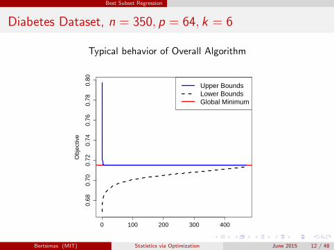
Diabetes Dataset, n = 350, p = 64, k = 6
Typical behavior of Overall Algorithm
0 100 200 300 400
0.68
0.70
0.72
0.74
0.76
0.78
0.80
k=6
Time (secs)
Obj
ectiv
e
Upper BoundsLower BoundsGlobal Minimum
Bertsimas (MIT) Statistics via Optimization June 2015 12 / 48

Best Subset Regression
Diabetes Dataset, n = 350, p = 64, k = 6
Typical behavior of Overall Algorithm
0 100 200 300 400
0.00
0.05
0.10
0.15
k=6
Time (secs)
MIO
−G
ap
Bertsimas (MIT) Statistics via Optimization June 2015 13 / 48

Best Subset Regression
First Order Method
Consider
minβ
g(β) = ‖y − Xβ‖22 subject to ‖β‖0 ≤ k
g(β) convex and
‖∇g(β)−∇g(β0)‖ ≤ ` · ‖β − β0‖.
This implies that for all L ≥ `
g(β) ≤ Q(β) = g(β0) + 〈∇g(β0),β − β0〉+L
2‖β − β0‖22
For the purpose of finding feasible solutions, we propose
minβ
Q(β) subject to ‖β‖0 ≤ k
Bertsimas (MIT) Statistics via Optimization June 2015 14 / 48

Best Subset Regression
Solution
Equivalent to
minβ
L
2
∥∥∥∥β − (β0 −1
L∇g(β0)
)∥∥∥∥22
− 1
2L‖∇g(β0)‖22 s.t. ‖β‖0 ≤ k
Reducing to
minβ‖β − u‖22 subject to ‖β‖0 ≤ k
Order: |u(1)| ≥ |u(2)| ≥ . . . ≥ |u(p)|,Optimal solution is β∗ = Hk(u), where Hk(u) retains the k largestelements of u and sets the rest to zero.
(Hk(u))i =
{ui , i ∈ {(1), . . . , (k)}0, otherwise.
Bertsimas (MIT) Statistics via Optimization June 2015 15 / 48

Best Subset Regression
First Order Algorithm
1 Initialize with a solution β0; m = 0.
2 m := m + 1.
3 β̃m+1 = Hk
(βm − 1
L∇g(βm)).
4 Perform a line search: λm+1 = argminλ g(λβ̃m+1)
βm+1 = λm+1β̃m+1
5 Repeat Steps 2-4 until ‖βm+1 − βm‖ ≤ ε.
Bertsimas (MIT) Statistics via Optimization June 2015 16 / 48

Best Subset Regression
Rate of Convergence
The sequence g(βm) converges to g(β) where
β = Hk
(β − 1
L∇g(β)
).
After M iterations:
minm=0,...,M
‖βm+1 − βm‖2 ≤2 · (g(β0)− g(β))
M · (L− `)
After M = O(1ε ) iterations the Algorithm converges.
Bertsimas (MIT) Statistics via Optimization June 2015 17 / 48

Best Subset Regression
Properties
Let Sm = {i : βm,i 6= 0, βm = (βm,1, . . . , βm,p)} be the support ofthe solution βm.
The support stabilizes, i.e., there exists an m∗ such that Sm+1 = Smfor all m ≥ m∗.
Once the support stabilizes, then the algorithm converges linearly.
The practical implication is that the algorithm scales to very largeproblems and converges very fast.
Bertsimas (MIT) Statistics via Optimization June 2015 18 / 48

Best Subset Regression
Quality of Solutions for n > p
Diabetes data: n = 350, p = 64.
Relative Accuracy = (falg − f∗)/f∗
maximum time 500 secs
kFirst Order MIO Cold Start MIO Warm Start
Accuracy Time Accuracy Time Accuracy Time
9 0.1306 1 0.0036 500 0 34620 0.1541 1 0.0042 500 0 7749 0.1915 1 0.0015 500 0 8757 0.1933 1 0 500 0 1
Bertsimas (MIT) Statistics via Optimization June 2015 19 / 48

Best Subset Regression
Quality of Solutions for n < p
Synthetic data: n = 50, p = 2000.
kFirst Order MIO Cold Start MIO Warm Start
Accuracy Time Accuracy Time Accuracy Time
4 0.1091 42.9 0.2910 500 0 65.95 0.1647 37.2 1.0510 500 0 72.26 0.6152 41.1 0.2769 500 0 77.1
SN
R=
3
7 0.7843 40.7 0.8715 500 0 160.78 0.5515 38.8 2.1797 500 0 295.89 0.7131 45.0 0.4204 500 0 96.0
4 0.2708 47.8 0 31 0 107.85 0.5072 45.6 0.7737 500 0 65.66 1.3221 40.3 0.5121 500 0 82.3
SN
R=
7
7 0.9745 40.9 0.7578 500 0 210.98 0.8293 40.5 1.8972 500 0 262.59 1.1879 44.2 0.4515 500 0 254.2
Bertsimas (MIT) Statistics via Optimization June 2015 20 / 48

Best Subset Regression
Sparsity Detection for n = 500, p = 100
0
10
20
30
40
1.742 3.484 6.967Signal−to−Noise Ratio
Num
ber
of N
onze
ros
Method
MIO
Lasso
Step
Sparsenet
Bertsimas (MIT) Statistics via Optimization June 2015 21 / 48

Best Subset Regression
Prediction Error = ‖Xβalg − Xβtrue‖22/‖Xβtrue‖2
2
0.00
0.05
0.10
0.15
0.20
0.25
1.742 3.484 6.967Signal−to−Noise Ratio
Pre
dict
ion
Per
form
ance
Method
MIO
Lasso
Step
Sparsenet
Bertsimas (MIT) Statistics via Optimization June 2015 22 / 48

Best Subset Regression
Sparsity Detection for n = 50, p = 2000
0
10
20
30
40
3 7 10Signal−to−Noise Ratio
Num
ber
Non
zero
s
Method
Lasso
First Order + MIO
First Order Only
Sparsenet
Bertsimas (MIT) Statistics via Optimization June 2015 23 / 48

Best Subset Regression
Prediction Error for n = 50, p = 2000
0.0
0.1
0.2
3 7 10Signal−to−Noise Ratio
Pre
dict
ion
Per
form
ance
Method
Lasso
First Order + MIO
First Order Only
Sparsenet
Bertsimas (MIT) Statistics via Optimization June 2015 24 / 48

Best Subset Regression
What did we learn?
For the case n > p, MIO+warm-starts finds provably optimalsolutions for n = 1000s, p = 100s in minutes.
For the case n < p, MIO+warm-starts finds solutions with betterprediction accuracy than Lasso or n = 100s, p = 1000s in minutesand proving optimality in hours.
MIO solutions have a significant edge in detecting sparsity, andoutperform Lasso in prediction accuracy.
Modern optimization (MIO+warm-starts) is capable of solving largescale instances.
Bertsimas (MIT) Statistics via Optimization June 2015 25 / 48

Regression: Art vs Science
The Art of Building Regression Models: Current Practice
Transform variables.
Pairwise scatterplots, correlation matrix.
Delete redundant variables.
Fit full model, delete variables with insignificant t-tests. Examineresiduals.
See if additional variables can be dropped/new variables brought in.
Validate the final model.
Bertsimas (MIT) Statistics via Optimization June 2015 26 / 48

Regression: Art vs Science
Aspirations: From Art to Science
Propose an algorithm (automated process) to build regression models.
Approach: Express all desirable properties as MIO constraints.
Bertsimas (MIT) Statistics via Optimization June 2015 27 / 48

Regression: Art vs Science
The initial MIO model
minβ,z
12‖y − Xβ‖22 + Γ‖β‖1 Robustness
s.t. zl ∈ {0, 1}, l = 1, . . . , p
−Mzl ≤ βl ≤Mzl , l = 1, . . . , pp∑
l=1
zl ≤ k Sparsity
z1 = . . . = zl ∀i = 1, . . . , l ∈ GSm, ∀m Group Sparsity
zi + zj ≤ 1 ∀(i , j) ∈ HC Pairwise Collinearity∑i∈Tm zi ≤ 1 ∀m Nonlinear Transform
Bertsimas (MIT) Statistics via Optimization June 2015 28 / 48

Regression: Art vs Science
Controlling Multicollinearity and Statistical Significance
Given a set S , we compute via bootstrap confidence levels of thevariables in S as well as the condition number of the model.
If the condition number is higher than desired or there are variablesthat are not statistically significant, we add the constraint:∑
j∈Szj ≤ |S| − 1
Iterate.
Bertsimas (MIT) Statistics via Optimization June 2015 29 / 48

Regression: Art vs Science
Contrast with existing practice
All desired properties are simultaneously enforced.
MIO does not have to choose which model properties to favor byperforming the steps in a certain order.
MIO is capable of handling datasets with more variables than amodeler can address manually.
Bertsimas (MIT) Statistics via Optimization June 2015 30 / 48
Regression: Art vs Science
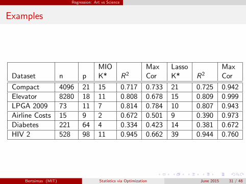
Examples
MIO Max Lasso MaxDataset n p K* R2 Cor K* R2 Cor
Compact 4096 21 15 0.717 0.733 21 0.725 0.942
Elevator 8280 18 11 0.808 0.678 15 0.809 0.999
LPGA 2009 73 11 7 0.814 0.784 10 0.807 0.943
Airline Costs 15 9 2 0.672 0.501 9 0.390 0.973
Diabetes 221 64 4 0.334 0.423 14 0.381 0.672
HIV 2 528 98 11 0.945 0.662 39 0.944 0.760
Bertsimas (MIT) Statistics via Optimization June 2015 31 / 48

Least Median Regression
Effect of Outliers in Regression
Least Squares (LS) estimator
β̂(LS)∈ argmin
β
n∑i=1
r2i , ri = yi − x′iβ
is adversely affected by a single outlier and has a limiting Breakdownpoint of 0 (Dohono & Huber ’83; Hampel ’75). (n→∞, and p fixed)
The Least Absolute Deviation (LAD) estimator has 0 breakdownpoint.
β̂(LAD)
∈ argminβ
n∑i=1
|ri |,
M-Estimators (Huber 1973) slightly improve the breakdown point
n∑i=1
ρ(ri ), ρ(r) symmetric function
Bertsimas (MIT) Statistics via Optimization June 2015 32 / 48

Least Median Regression
Least Median Regression
Least Median of Squares (LMS) estimator (Rousseew (1984) )
β̂(LMS)
∈ argminβ
(mediani=1,...,n
|ri |).
LMS highest possible breakdown point of almost 50%.
More generally, Least Quantile of Squares (LQS) estimator:
β̂(LQS)
∈ argminβ
|r(q)|,
where, r(q) is the qth ordered absolute residual:
|r(1)| ≤ |r(2)| ≤ . . . ≤ |r(n)|.
Bertsimas (MIT) Statistics via Optimization June 2015 33 / 48

Least Median Regression
LMS Computation : State of the art
LMS problem is NP-hard (Bernholt 2005).
Exact Algorithms
Enumeration based, branch and bound, scale like O(np).Practically Exact algorithms scale up to n = 50, p = 5.
Heuristic Algorithms
Based on heuristic subsampling / local searches.Practically scale significantly better, but no guarantees.
Bertsimas (MIT) Statistics via Optimization June 2015 34 / 48

Least Median Regression
Problem we address
Solve the following problem:
minβ|r(q)|,
where, ri = yi − x′iβ, q is a quantile.
Our approach extends to
minβ|r(q)|, subject to Aβ ≤ b (and/or ‖β‖22 ≤ δ)
Bertsimas (MIT) Statistics via Optimization June 2015 35 / 48

Least Median Regression
Overview of our approach
1 Write the LMS problem as a MIO.
2 Using first order methods we find feasible solutions which we use aswarm-starts.
3 First order solutions serve as warm-starts that enhance running times.
Bertsimas (MIT) Statistics via Optimization June 2015 36 / 48

Least Median Regression
MIO Formulation
Notation:|r(1)| ≤ |r(2)| ≤ . . . ≤ |r(n)|.
Step 1: Introduce binary variables zi , i = 1, . . . , n such that:
zi =
{1, if |ri | ≤ |r(q)|,0, otherwise.
Step 2: Use auxiliary continuous variables µi , µi ≥ 0 such that:
|ri | − µi ≤ |r(q)| ≤ |ri |+ µi , i = 1, . . . , n,
with the conditions:
If |ri | ≥ |r(q)|, then µi = 0, µi ≥ 0,
and if |ri | ≤ |r(q)|, then µi = 0, µi ≥ 0.
Bertsimas (MIT) Statistics via Optimization June 2015 37 / 48

Least Median Regression
MIO Formulation
min γ
subject to |ri |+ µi ≥ γ, i = 1 . . . , n
γ ≥ |ri | − µi , i = 1 . . . , n
Muzi ≥ µi , i = 1, . . . , n
M`(1− zi ) ≥ µi , i = 1, . . . , nn∑
i=1
zi = q
µi ≥ 0, i = 1, . . . , n
µi ≥ 0, i = 1, . . . , n
zi ∈ {0, 1}, i = 1, . . . , n,
where γ, zi , µi , µi , i = 1, . . . , n are decision variables and Mu,M` are Big-Mconstants.
Bertsimas (MIT) Statistics via Optimization June 2015 38 / 48

Least Median Regression
SOS-formulation
min γ
subject to |ri | − γ = µi − µi , i = 1 . . . , nn∑
i=1
zi = q
γ ≥ µi , i = 1 . . . , n
µi ≥ 0, i = 1 . . . , n
µi ≥ 0, i = 1, . . . , n
(µi , µi ) : SOS-1, i = 1, . . . , n
(zi , µi ) : SOS-1, i = 1, . . . , n
zi ∈ {0, 1}, i = 1, . . . , n.
Bertsimas (MIT) Statistics via Optimization June 2015 39 / 48

Least Median Regression
Typical Evolution of MIO
0 20 40 60 80
0.0
0.1
0.2
0.3
0.4
Alcohol Data; (n,p,q) = (44,5,31)
Time (s)
Obj
ectiv
e V
alue
Upper BoundsLower BoundsOptimal Solution
0 200 400 600 8000.
00.
10.
20.
30.
4
Alcohol Data; (n,p,q) = (44,7,31)
Time (s)
Obj
ectiv
e V
alue
Upper BoundsLower BoundsOptimal Solution
Bertsimas (MIT) Statistics via Optimization June 2015 40 / 48

Least Median Regression
First Order Method
Writing r(q) = y(q) − x′(q)β
|y(q) − x′(q)β| =
q+1∑i=1
|y(i) − x′(i)β|︸ ︷︷ ︸Hq+1(β)
−q∑
i=1
|y(i) − x′(i)β|︸ ︷︷ ︸Hq(β)
,
The function Hm(β) is convex in β (sum of piecewise convex linearfunctions)
Hm(β) := maxw
n∑i=1
wi |yi − x′iβ|
subject to
n∑i=1
wi = m
0 ≤ wi ≤ 1, i = 1, . . . , n.
Bertsimas (MIT) Statistics via Optimization June 2015 41 / 48

Least Median Regression
Expressing Hq+1(β) a LO
Hq+1(β) can be expressed as
Hq+1(β) := maxw
n∑i=1
wi |yi − x′iβ|
subject to
n∑i=1
wi = q + 1
0 ≤ wi ≤ 1, i = 1, . . . , n.
By taking the dual and invoking strong duality, we have:
Hq+1(β) = minθ,ν
θ (q + 1) +n∑
i=1
νi
subject to θ + νi ≥ |yi − x′iβ|, i = 1, . . . , n
νi ≥ 0, i = 1, . . . , n.
Bertsimas (MIT) Statistics via Optimization June 2015 42 / 48

Least Median Regression
Expressing Hq(β)
Hq(β) can be expressed as
Hm(β) := maxw
n∑i=1
wi |yi − x′iβ|
subject to
n∑i=1
wi = m
0 ≤ wi ≤ 1, i = 1, . . . , n.
Subgradients:
∂ Hq(β) = conv
{n∑
i=1
w∗i sgn(yi − x′iβ)xi : w∗ ∈ argmaxw∈Wq
L(β,w)
},
Hq(β) ≈ Hq(βk) + 〈∂Hq(βk),β − βk〉.
Bertsimas (MIT) Statistics via Optimization June 2015 43 / 48

Least Median Regression
Combining the pieces.....
Given a current solution βk , we find βk+1:
minν,θ,β
θ(q + 1) +n∑
i=1
νi − 〈∂Hq(βk),β〉
subject to θ + νi ≥ |yi − x′iβ|, i = 1, . . . , n
νi ≥ 0, i = 1, . . . , n.
Termination(|y(q) − x′(q)βk | − |y(q) − x′(q)βk+1|
)≤ Tol · |y(q) − x′(q)βk |
The algorithm converges in O(1/ε) to a stationary point (local optimalsolution).
Bertsimas (MIT) Statistics via Optimization June 2015 44 / 48

Least Median Regression
Impact of Warm-Starts
Evolution of MIO (cold-start) [top] vs (warm-start) [bottom]
0 500 1000 1500 2000
010
2030
4050
Time (s)
Objec
tive Va
lue
Upper BoundsLower BoundsOptimal Solution
0 500 1000 1500 2000
02
46
810
12
Time (s)
Objec
tive Va
lue
Upper BoundsLower BoundsOptimal Solution
n = 501, p = 5, synthetic example
Bertsimas (MIT) Statistics via Optimization June 2015 45 / 48

Least Median Regression
Conclusions
MIO+warm-starts solves to provable optimality problems of medium(n = 500) size problems in under two hours.
MIO+warm-starts finds high quality solutions for large (n = 10, 000) scaleproblems in under two hours outperforming all state of the art algorithmsthat are publicly available for the LQS problem.
For problems of this size (n = 10, 000), MIO does not provide a certificate ofoptimality in a reasonable amount of time.
Bertsimas (MIT) Statistics via Optimization June 2015 46 / 48

Least Median Regression
Remarks on Complexity:
A key requirement of a theory is to be positively correlated with empiricalevidence.
Consider the Simplex method and solving the TSP.
A 200 billion speed up forces us to reconsider what is tractable.
Definition: A problem is tractable if it can be solved for sizes and in timesthat are appropriate for the application.
Online trading problems need to be solved in milliseconds.
Regression problems used for planning need to be solved in minutes or inhours.
Asymptotic polynomial solvability or NP-hardness is not relevant under thisdefinition.
Bertsimas (MIT) Statistics via Optimization June 2015 47 / 48

Least Median Regression
Remarks on Statistics
Problems in statistics and machine learning considered intractable ageneration ago are now tractable.
Lasso is a robustness property not a sparsity inducing property as widelybelieved.
In comparison to Lasso, MIO provides a significance edge for detectingsparsity as well as an edge on predictive accuracy.
It is my view that the time to include MIO in statistics curricula has come.
Correspondingly, I will be teaching a first year graduate level class at MIT:Statistics under a modern optimization lens.
Bertsimas (MIT) Statistics via Optimization June 2015 48 / 48
Top Related