


Languages
Pages
Legal


SMUT EPIDEMIOLOGY SRDC-funded project
Rob MagareyBSES Limited, Tully

Epidemiology
Definition
Study of the spread, build up and effect of an epidemic

Smut epidemic in Queensland
• First detection: 9th June 2006, Isis
– single side-shoot– nothing known of epidemic
history• How many farms?• Which parts of the district?• What varieties? etc
• Other detections (2006)– Mackay: 7th November – Herbert: 15th December

Smut epidemics: what we knew!
• Smut can spread fast
• Is affected by climate– Wetter conditions can slow build up– Warmer temperatures favour the
disease– Hot, dry (irrigated) is most suitable
• Inoculum can travel a long way– 1000s km– but heaviest inoculum pressure is
within just a few metres of an infested crop
• Yield losses: – 0.6% loss for each 1% infested
stalks = 62% yield loss in HS

Smut: what we knew!
• Our commercial varieties were highly susceptible
• That many of the best canes were also HS
• It would be difficult to replace crops quickly to establish resistant crops
• Accessing disease-free plant sources was very important since smut can be planted in apparently healthy looking cane

Smut epidemics: what we didn’t know
• When it would be detected in Northern, Burdekin, NSW etc
• How long it would take to reach each farm in affected districts
• How quickly the disease would build up in HS crops
• When significant yield losses would start occurring in infested crops
• What influence climate would have
• What level of resistance was needed in each district to restrict losses
• How our potential replacement varieties would go in each district

Project (farmer) questions
Immediate questions
• How fast will it reach my farm? (spread)
• How quickly will it build up in my HS crops (build-up)
• How fast will I need to terminate the crop
before losses occur?
Additional questions (project extension)
• How will the ‘I’ varieties withstand the epidemic?
• What yield losses are / will occur?
• When will the epidemic pass?

Epidemic J curve
0
100
200
300
400
500
600
700
800
900
1000
1100
0 100 200 300 400 500 600 700 800 900 1000
Time
Num
ber
of fa
rms
Slow start
Fast finish
Epidemics

Epidemiology methods
Two initial focus areas
• Smut spread Monitoring a non-diseased farm
network
• Smut build up increase in % stools in example
susceptible crops

Smut spread

Smut spread
Two strategies2. Smut-free farm network
3. Farmer reporting
Smut-free network• Un-infested farms were
selected• Networks in each of
Bundaberg, Mackay, Herbert• Inspected regularly for smut• Speed of spread monitored

Predicted smut spread
Bundaberg
y = 0.1183x - 0.4421
R2 = 0.99
-20
0
20
40
60
80
100
0 100 200 300 400 500 600 700
Days
% f
arm
s in
fes
ted
Predicted 100% farms = April 2009

Smut spread
Second predictorKnown smut farms - farmer
reporting
• Recordings of all reported smut farms (not just study farms)
• Database maintained• Provided ‘real district’ data
– Worked to a point• when smut more commonplace,
reporting ceased
• Plotted data vs time

Smut farms reported
Herbert: predicted 100% farms infested
y = 6.924e0.0074x
R2 = 0.9756
0
100
200
300
400
500
600
700
800
900
1000
0 100 200 300 400 500 600 700 800
Days (since December 2006)
Nu
mb
er o
f fa
rms
December 2006
April 2008
100% infestation
October 2008

Mackay
Mackay: predicted 100% farms infested
y = 4.0697e0.007x
R2 = 0.9662
0
200
400
600
800
1000
1200
0 100 200 300 400 500 600 700 800 900
Days (after December 2006)
Nu
mb
er
of
farm
s
November 2006
April 2008
February 2009
100% infestation

Bundaberg-Isis
Bundaberg-Isis predicted 100% farms infested
y = 29.213e0.0031x
R2 = 0.9644
0
100
200
300
400
500
600
700
800
900
0 100 200 300 400 500 600 700 800 900 1000 1100 1200
Days (since June 2006)
Nu
mb
er f
arm
s sm
ut-
infe
sted 100% infestation
April 2009April 2008
June 2006


Smut build-up

Smut build up ‘in-crop’
• Example HS crops selected
• Individual stools monitored (+ or – smut)
• Data recorded using GPS• Stools mapped
• Increase in smut calculated
• Escalation rates determined

Q205 Bundaberg

Q205 Bundaberg

Q205 Bundaberg

Q205 Bundaberg

Q205 Bundaberg

Q205 Bundaberg

Crop build up conclusions
Build up rates• variable
• depending on initial smut crop levels• local environment• highest when smut is ‘planted’
• 7-11 fold stool increase / year– compares to 1-2 fold in Louisiana
• 1-3 years: first detection to predicted ploughout!• 5% infested stools

Smut yield losses

Q174: March 2010

Yield losses
Our whole aim in the smut program, working in– epidemiology– variety resistance screening– spore trapping– extension
was to avoid high smut incidence in HS varieties
• and the high associated yield losses!
We wanted to pre-warn farmers of the potential yield effects

Quantifying losses
Strategy: choose 7 plots in a crop with varying smut levels– Assess yield in each plot– Relate smut severity to yield
• Identified a badly-affected 2009 crop in the Herbert (Abergowrie)
• Highly susceptible Q157
Yield losses
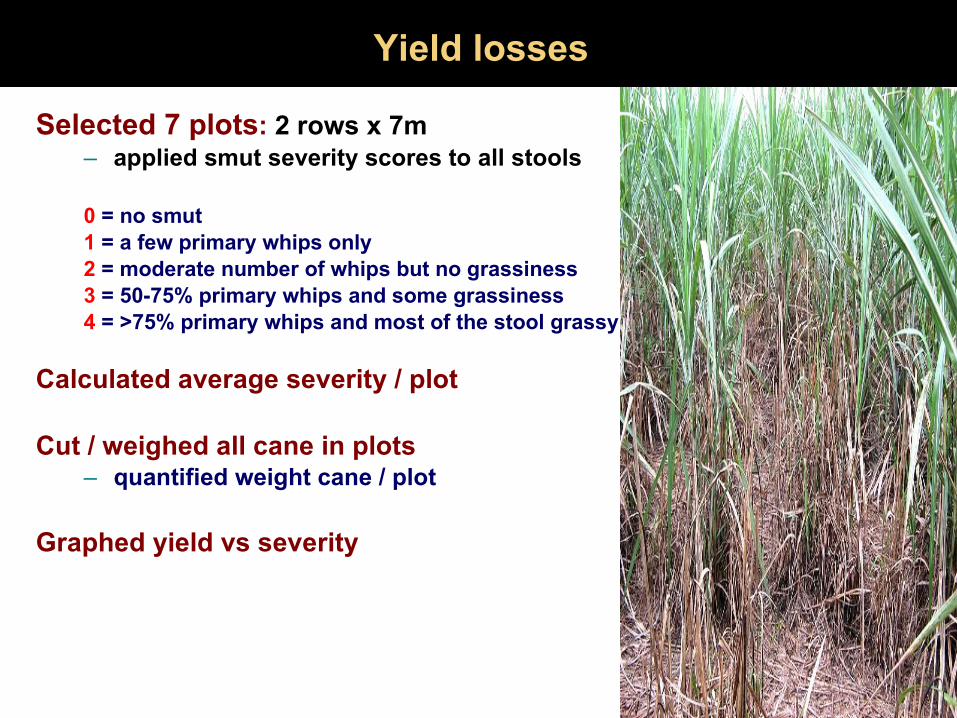
Selected 7 plots: 2 rows x 7m– applied smut severity scores to all stools
0 = no smut1 = a few primary whips only2 = moderate number of whips but no grassiness3 = 50-75% primary whips and some grassiness4 = >75% primary whips and most of the stool grassy
Calculated average severity / plot
Cut / weighed all cane in plots– quantified weight cane / plot
Graphed yield vs severity

Q157 Yield loss
y = -15.567x + 99.657
40.0
50.0
60.0
70.0
80.0
90.0
100.0
0.0 0.5 1.0 1.5 2.0 2.5 3.0 3.5
Smut severity
Yie
ld (
ton
ne
s ca
ne
/ h
a)
Smut severity vs cane yield

Yield losses
Using these data
Theoretical maximum yield loss:
• score ‘0’ vs ‘4’
62%
= same as predicted at start of Childers epidemic!

Yield losses
What losses did the farmer suffer in that crop (whole crop)?
• Depends on average crop severity• Selected 20 plots scattered randomly
through the crop (10m length)• Scored all stools in all plots• Found average severity
= average whole crop severity
Related yield loss estimate x severity
– to estimate total crop losses in that particular crop

• Average severity across whole crop– 20 plots
• Mean severity score = 1.6 (0 to 4 severity scale)
• Related to yield • using the previous graph
The average smut-induced yield loss for that whole crop = 26%.
Yield losses

Variety effectsField

Strong field variety effects
Variety # crops Variety # cropsQ158 154 Q220 3
Q174 151 Q233 3
Q157 67 Q115 3
Q204 18 Q152 3
Q186 14 Q164 3
Q194 14 Q216 3
Q162 13 Q172 2
Q166 10 Q127 2
Q195 10 Q138 2
Q200 5 Q99 1
Argos 5 KQ228 1
Q179 5 Q219 1
Q190 3 Q183 1
Herbert

What level of resistance is needed?
• Natural spread trial planted in Mackay
– Varieties varying in resistance – Included important ‘replacement’ canes– Planted ‘clean’
• Monitored disease buildup vs HS canes• Worst affected farm in Mackay

Mackay natural spread – April 2009
0
10
20
30
40
50
60
70
Q157 Q209 Q190 Q138 Q226 Q200 Q208 Q205ss Q205 Q170 Q171 Q135 Q183
Variety
% s
too
ls in
fest
ed

• Highly susceptible canes – Severe smut very quickly– Disaster!
• Susceptible (7-8)– Not so fast
• Intermediate canes– pretty good– especially Q183, Q135,
Q208
• Resistant canes– No problem
Field resistance
0
10
20
30
40
50
60
70
Q157 Q209 Q190 Q138 Q226 Q200 Q208 Q205ss Q205 Q170 Q171 Q135 Q183
Variety
% s
too
ls in
fest
ed

Q208: a major variety!
• Some have expressed concern about disease levels
• In Mackay – some significant disease (around 1.5% disease)
• Herbert – one report of 9% infested stools
• But following crops have had low smut levels– this also seen in the Ord
• No problem with this variety!

When will the epidemic pass?
Epidemic modelling

Epidemic modelling
• Based on weighted parameter– % S, I and R crops: district x year– plus estimated smut severity
• Calculated parameter: ‘relative smut’ - smut indicator
• Models: guide to when the maximum smut stress on ‘I’ varieties

Herbert district
Relative smut
0
50000
100000
150000
200000
250000
300000
350000
400000
2005 2006 2007 2008 2009 2010 2011 2012 2013
Year
Rel
ativ
e sm
ut

Epidemic modelling
• RISE of the epidemic– principally about smut
• spread• escalation
– in HS crops (plenty around)
• FALL of the epidemic– almost wholly to do with: -
• elimination of HS crops

Bundaberg-Childers
Relative smut
0
50000
100000
150000
200000
250000
2005 2006 2007 2008 2009 2010 2011 2012 2013
Year
Rel
ativ
e sm
ut

Epidemic modelling
Bundaberg-Childers
• Similar pattern to the Herbert• Peak in 2009 (a little earlier)
– More rapid replacement of susceptibles
Peak smaller than Herbert

Smut comparison x district
0
50000
100000
150000
200000
250000
300000
350000
400000
2004 2006 2008 2010 2012 2014 2016
Year
Re
lati
ve s
mu
t
Herbert
Bundaberg
Burdekin

Herbert – estimated losses
Estimated yield losses from smut - Herbert
0
50,000
100,000
150,000
200,000
250,000
300,000
350,000
400,000
2009 2010 2011 2012
Year
To
nn
es

Yield losses
Herbert region losses: • 2009 crop losses: estimated at
250,000 tonnes
• 2010 losses: estimated at
>300,000 tonnes cane
• In 2010: > 30% of Herbert crop supplied by S varieties, and – smut likely to be severe in HS crops.

Important management points
• Maintain transition to resistant varieties – if too slow, there will be high direct
losses, and – maximum inoculum pressure on
intermediates
• Industry needs to make common sense decisions on which crops to terminate

Conclusions
• This is ‘crunch’ time - yield loss
phase• Losses will be significant in
Herbert, Mackay and Bundaberg in 2010 and 2011
• Largely confined to the HS varieties
Urgent need to transition out of HS to avoid yield losses!

Overall conclusions
• Smut: 2-3 years to spread to all farms in district
• Significant losses: within 3 years from first finding of smut in a crop (susceptible)– 10-fold stool increase each
year
• Some intermediates will be OK
• Smut losses: a little slower to occur than anticipated
Top Related