


Languages
Pages
Legal


SPSS Instructions for Introduction to Biostatistics
Larry Winner
Department of Statistics
University of Florida
SPSS Windows• Data View
– Used to display data
– Columns represent variables
– Rows represent individual units or groups of units that share common values of variables
• Variable View– Used to display information on variables in dataset
– TYPE: Allows for various styles of displaying
– LABEL: Allows for longer description of variable name
– VALUES: Allows for longer description of variable levels
– MEASURE: Allows choice of measurement scale
• Output View– Displays Results of analyses/graphs

Data Entry Tips I
• For variables that are not identifiers (such as name, county, school, etc), use numeric values for levels and use the VALUES option in VARIABLE VIEW to give their levels. Some procedures require numeric labels for levels. SPSS will print the VALUES on output
• For large datasets, use a spreadsheet such as EXCEL which is more flexible for data entry, and import the file into SPSS
• Give descriptive LABEL to variable names in the VARIABLE VIEW
• Keep in mind that Columns are Variables, you don’t want multiple columns with the same variable
Data Entry/Analysis Tips II
• When re-analyzing previously published data, it is often possible to have only a few outcomes (especially with categorical data), with many individuals sharing the same outcomes (as in contingency tables)
• For ease of data entry:– Create one line for each combination of factor levels
– Create a new variable representing a COUNT of the number of individuals sharing this “outcome”
• When analyzing data Click on:– DATA WEIGHT CASES WEIGHT CASES BY
– Click on the variable representing COUNT
– All subsequent analyses treat that outcome as if it occurred COUNT times

Example 1.3 - Grapefruit Juice Study
crcl38667499806480
120
To import an EXCEL file, click on:
FILE OPEN DATA then change FILES OF TYPE to EXCEL (.xls)
To import a TEXT or DATA file, click on:
FILE OPEN DATA then change FILES OF TYPE to TEXT (.txt) or
DATA (.dat)
You will be prompted through a series of dialog boxes to import dataset

Descriptive Statistics-Numeric Data
• After Importing your dataset, and providing names to variables, click on:
• ANALYZE DESCRIPTIVE STATISTICS DESCRIPTIVES
• Choose any variables to be analyzed and place them in box on right
• Options include:
n
S
Sn
yyS
yn
yy
n
ii
n
ii
n
ii
:Mean S.E.
:Variance 1
:deviation Std.
:Sum :Mean
21
2
1
1

Example 1.3 - Grapefruit Juice Study
Descriptive Statistics
8 38 120 621 77.63 8.63 24.401 595.411
8
CRCL
Valid N (listwise)
Statistic Statistic Statistic Statistic Statistic Std. Error Statistic Statistic
N Minimum Maximum Sum Mean Std.Deviation
Variance
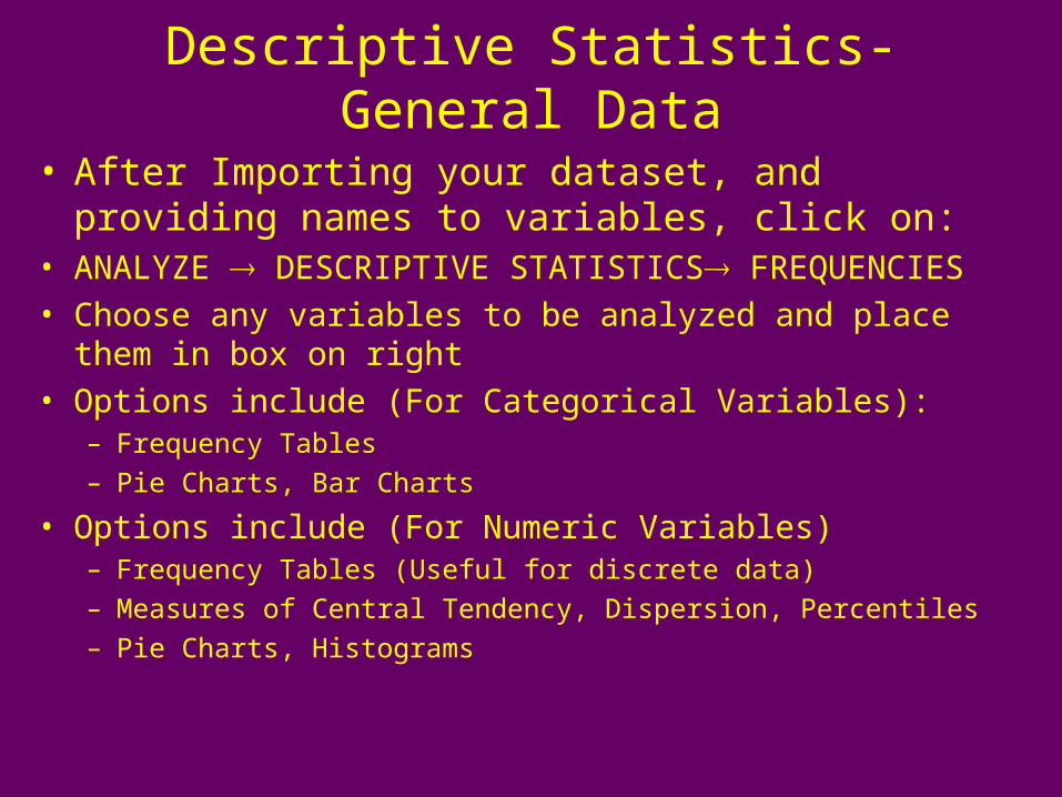
Descriptive Statistics-General Data
• After Importing your dataset, and providing names to variables, click on:
• ANALYZE DESCRIPTIVE STATISTICS FREQUENCIES
• Choose any variables to be analyzed and place them in box on right
• Options include (For Categorical Variables):– Frequency Tables
– Pie Charts, Bar Charts
• Options include (For Numeric Variables)– Frequency Tables (Useful for discrete data)
– Measures of Central Tendency, Dispersion, Percentiles
– Pie Charts, Histograms

Example 1.4 - Smoking Status
SMKSTTS
1990 37.9 37.9 37.9
1063 20.3 20.3 58.2
609 11.6 11.6 69.8
1332 25.4 25.4 95.2
253 4.8 4.8 100.0
5247 100.0 100.0
Never Smoked
Quit > 10 Years Ago
Quit < 10 Years Ago
Current Cigarette Smoker
Other Tobacco User
Total
ValidFrequency Percent Valid Percent
CumulativePercent
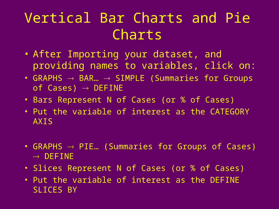
Vertical Bar Charts and Pie Charts
• After Importing your dataset, and providing names to variables, click on:
• GRAPHS BAR… SIMPLE (Summaries for Groups of Cases) DEFINE
• Bars Represent N of Cases (or % of Cases)
• Put the variable of interest as the CATEGORY AXIS
• GRAPHS PIE… (Summaries for Groups of Cases) DEFINE
• Slices Represent N of Cases (or % of Cases)
• Put the variable of interest as the DEFINE SLICES BY

Example 1.5 - Antibiotic Study
OUTCOME
54321
Co
un
t
80
60
40
20
0
5
4
3
2
1

Histograms
• After Importing your dataset, and providing names to variables, click on:
• GRAPHS HISTOGRAM
• Select Variable to be plotted
• Click on DISPLAY NORMAL CURVE if you want a normal curve superimposed (see Chapter 3).
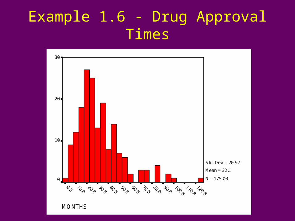
Example 1.6 - Drug Approval Times
MONTHS
30
20
10
0
Std. Dev = 20.97
Mean = 32.1
N = 175.00
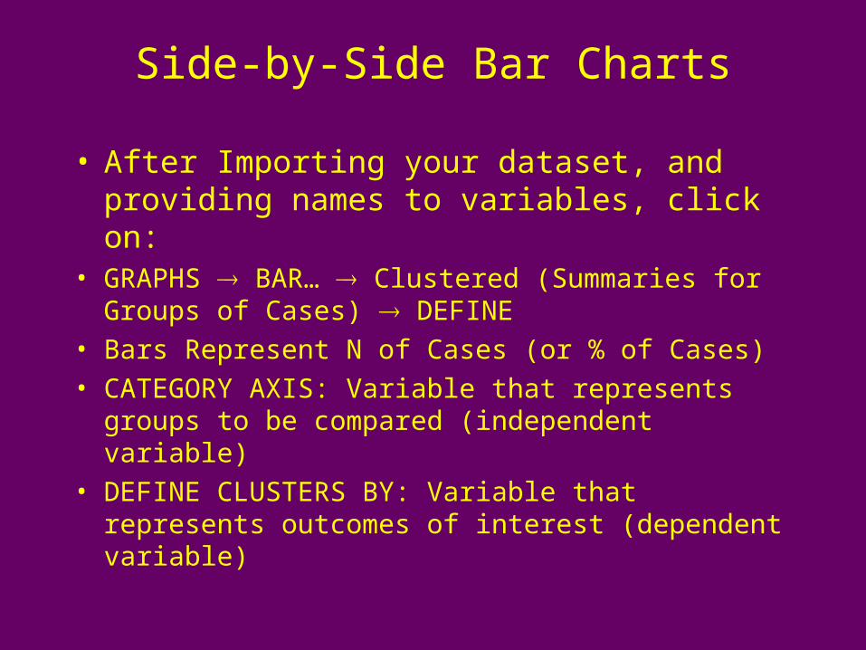
Side-by-Side Bar Charts
• After Importing your dataset, and providing names to variables, click on:
• GRAPHS BAR… Clustered (Summaries for Groups of Cases) DEFINE
• Bars Represent N of Cases (or % of Cases)
• CATEGORY AXIS: Variable that represents groups to be compared (independent variable)
• DEFINE CLUSTERS BY: Variable that represents outcomes of interest (dependent variable)

Example 1.7 - Streptomycin Study
TRT
21
Co
un
t30
20
10
0
OUTCOME
1
2
3
4
5
6

Scatterplots
• After Importing your dataset, and providing names to variables, click on:
• GRAPHS SCATTER SIMPLE DEFINE
• For Y-AXIS, choose the Dependent (Response) Variable
• For X-AXIS, choose the Independent (Explanatory) Variable

Example 1.8 - Theophylline Clearance
DRUG
3.53.02.52.01.51.0.5
TH
CL
RN
CE8
7
6
5
4
3
2
1
0
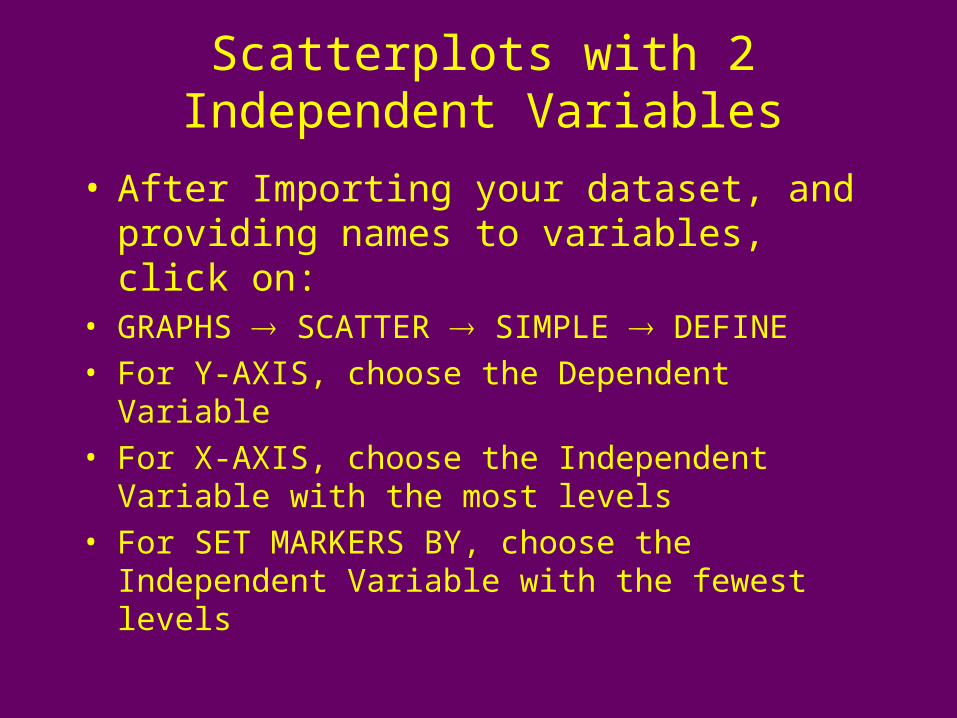
Scatterplots with 2 Independent Variables
• After Importing your dataset, and providing names to variables, click on:
• GRAPHS SCATTER SIMPLE DEFINE
• For Y-AXIS, choose the Dependent Variable
• For X-AXIS, choose the Independent Variable with the most levels
• For SET MARKERS BY, choose the Independent Variable with the fewest levels

Example 1.8 - Theophylline Clearance
SUBJECT
1614121086420
TH
CL
RN
CE
8
7
6
5
4
3
2
1
0
DRUG
Tagamet
Pepcid
Placebo

Contingency Tables for Conditional Probabilities
• After Importing your dataset, and providing names to variables, click on:
• ANALYZE DESCRIPTIVE STATISTICS CROSSTABS
• For ROWS, select the variable you are conditioning on (Independent Variable)
• For COLUMNS, select the variable you are finding the conditional probability of (Dependent Variable)
• Click on CELLS
• Click on ROW Percentages

Example 1.10 - Alcohol & Mortality
WINE * DEATH Crosstabulation
10535 2155 12690
83.0% 17.0% 100.0%
521 74 595
87.6% 12.4% 100.0%
11056 2229 13285
83.2% 16.8% 100.0%
Count
% within WINE
Count
% within WINE
Count
% within WINE
0
1
WINE
Total
0 1
DEATH
Total
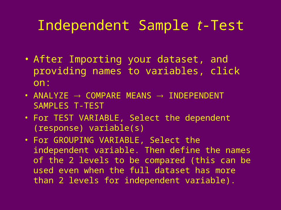
Independent Sample t-Test
• After Importing your dataset, and providing names to variables, click on:
• ANALYZE COMPARE MEANS INDEPENDENT SAMPLES T-TEST
• For TEST VARIABLE, Select the dependent (response) variable(s)
• For GROUPING VARIABLE, Select the independent variable. Then define the names of the 2 levels to be compared (this can be used even when the full dataset has more than 2 levels for independent variable).
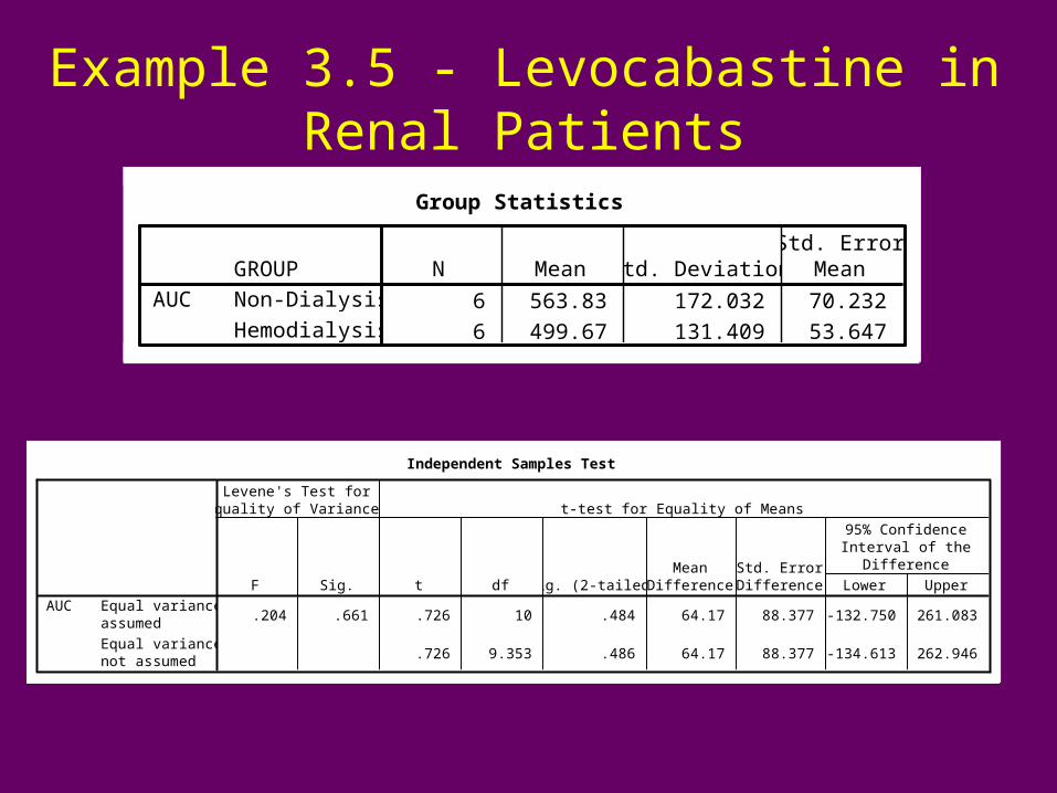
Example 3.5 - Levocabastine in Renal Patients
Group Statistics
6 563.83 172.032 70.232
6 499.67 131.409 53.647
GROUPNon-Dialysis
Hemodialysis
AUCN Mean Std. Deviation
Std. ErrorMean
Independent Samples Test
.204 .661 .726 10 .484 64.17 88.377 -132.750 261.083
.726 9.353 .486 64.17 88.377 -134.613 262.946
Equal variancesassumed
Equal variancesnot assumed
AUCF Sig.
Levene's Test forEquality of Variances
t df Sig. (2-tailed)Mean
DifferenceStd. ErrorDifference Lower Upper
95% ConfidenceInterval of the
Difference
t-test for Equality of Means

Wilcoxon Rank-Sum/Mann-Whitney Tests
• After Importing your dataset, and providing names to variables, click on:
• ANALYZE NONPARAMETRIC TESTS 2 INDEPENDENT SAMPLES
• For TEST VARIABLE, Select the dependent (response) variable(s)
• For GROUPING VARIABLE, Select the independent variable. Then define the names of the 2 levels to be compared (this can be used even when the full dataset has more than 2 levels for independent variable).
• Click on MANN-WHITNEY U

Example 3.6 - Levocabastine in Renal Patients
Ranks
6 7.50 45.00
6 5.50 33.00
12
GROUPNon-Dialysis
Hemodialysis
Total
AUCN Mean Rank Sum of Ranks
Test Statisticsb
12.000
33.000
-.962
.336
.394a
Mann-Whitney U
Wilcoxon W
Z
Asymp. Sig. (2-tailed)
Exact Sig. [2*(1-tailedSig.)]
AUC
Not corrected for ties.a.
Grouping Variable: GROUPb.
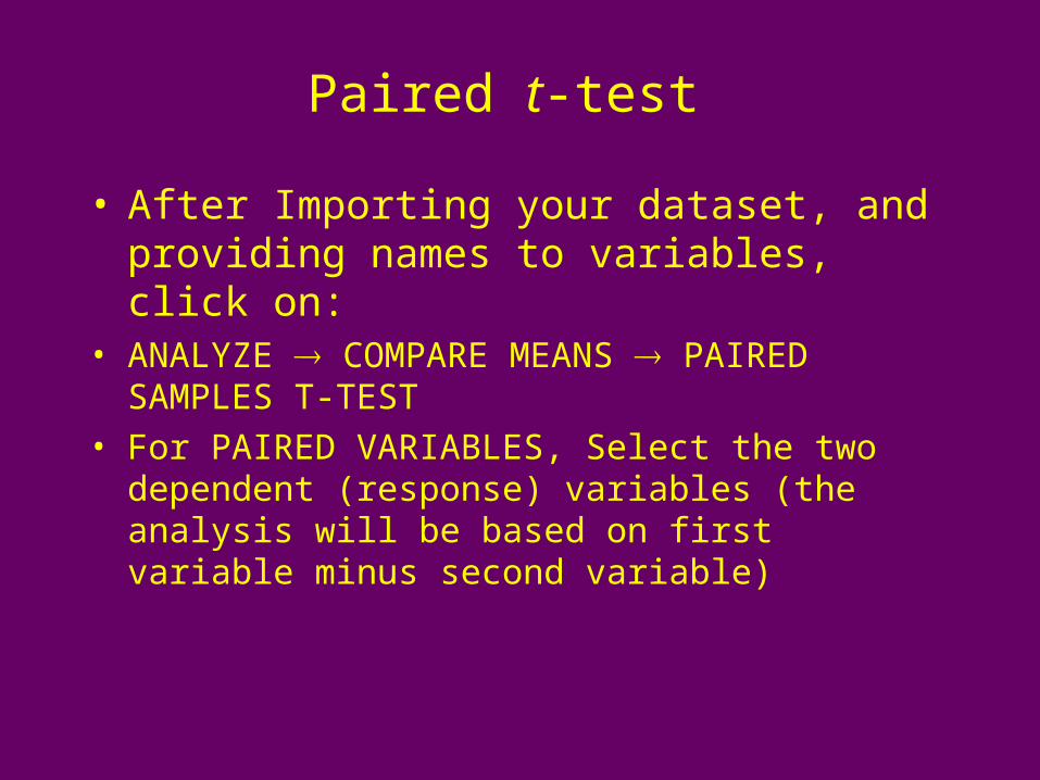
Paired t-test
• After Importing your dataset, and providing names to variables, click on:
• ANALYZE COMPARE MEANS PAIRED SAMPLES T-TEST
• For PAIRED VARIABLES, Select the two dependent (response) variables (the analysis will be based on first variable minus second variable)
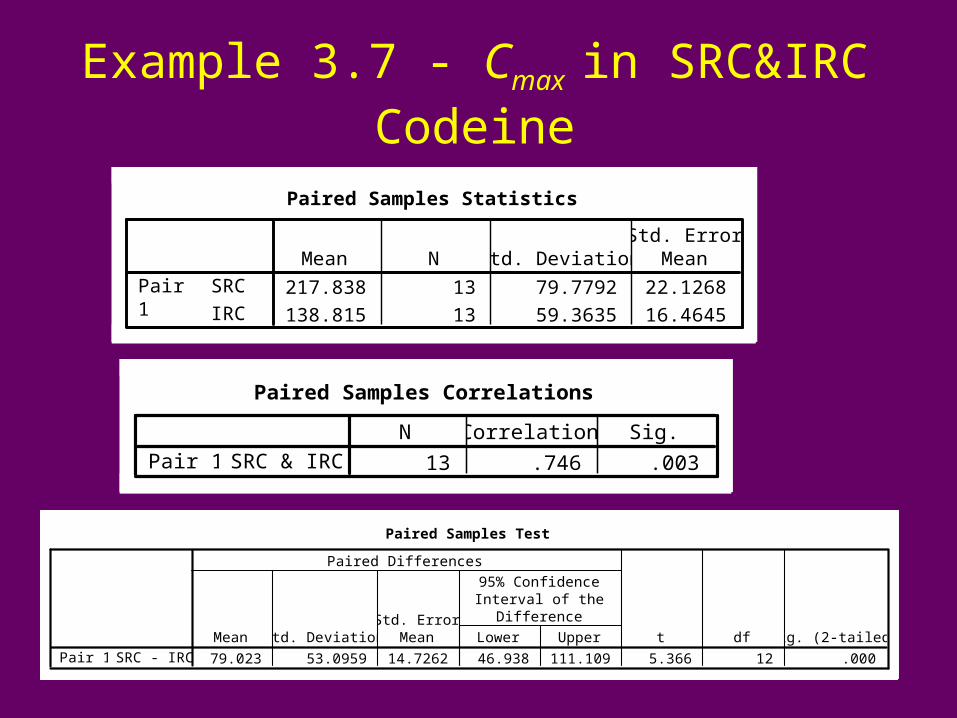
Example 3.7 - Cmax in SRC&IRC Codeine
Paired Samples Statistics
217.838 13 79.7792 22.1268
138.815 13 59.3635 16.4645
SRC
IRC
Pair1
Mean N Std. DeviationStd. Error
Mean
Paired Samples Correlations
13 .746 .003SRC & IRCPair 1N Correlation Sig.
Paired Samples Test
79.023 53.0959 14.7262 46.938 111.109 5.366 12 .000SRC - IRCPair 1Mean Std. Deviation
Std. ErrorMean Lower Upper
95% ConfidenceInterval of the
Difference
Paired Differences
t df Sig. (2-tailed)

Wilcoxon Signed-Rank Test
• After Importing your dataset, and providing names to variables, click on:
• ANALYZE NONPARAMETRIC TESTS 2 RELATED SAMPLES
• For PAIRED VARIABLES, Select the two dependent (response) variables (be careful in determining which order the differences are being obtained, it will be clear on output)
• Click on WILCOXON Option

Example 3.8 - t1/2SS
in SRC&IRC Codeine
Ranks
9a 6.89 62.00
3b 5.33 16.00
1c
13
Negative Ranks
Positive Ranks
Ties
Total
IRC - SRCN Mean Rank Sum of Ranks
IRC < SRCa.
IRC > SRCb.
IRC = SRCc.
Test Statisticsb
-1.805a
.071
Z
Asymp. Sig. (2-tailed)
IRC - SRC
Based on positive ranks.a.
Wilcoxon Signed Ranks Testb.
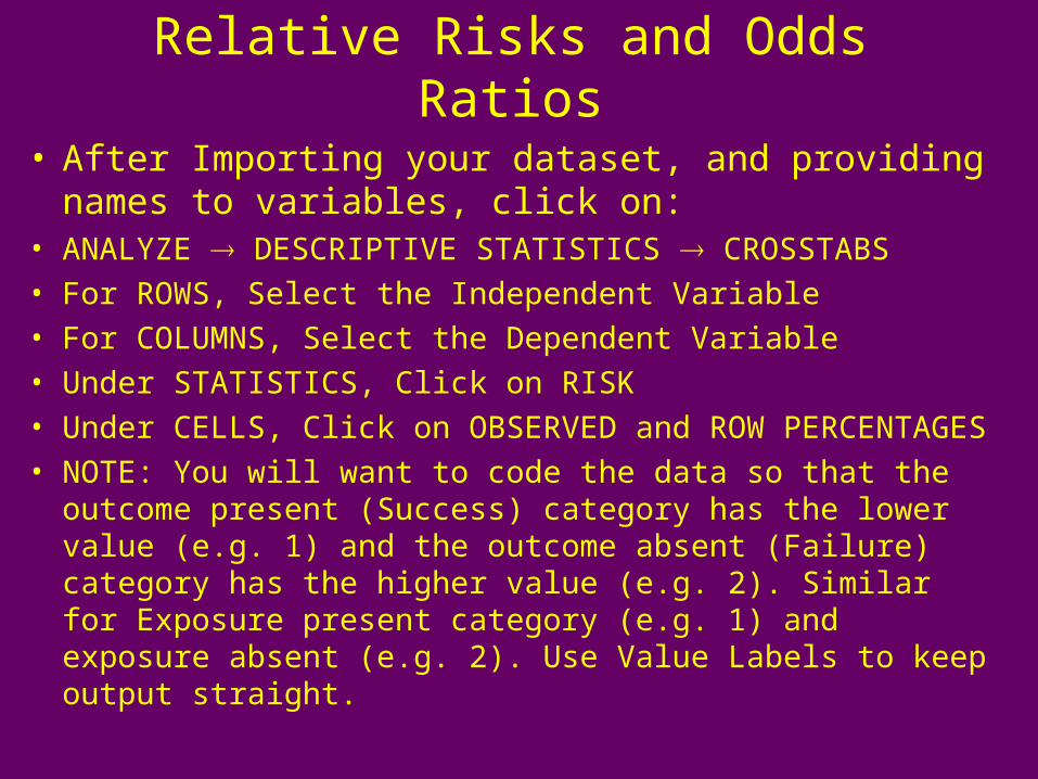
Relative Risks and Odds Ratios
• After Importing your dataset, and providing names to variables, click on:
• ANALYZE DESCRIPTIVE STATISTICS CROSSTABS
• For ROWS, Select the Independent Variable
• For COLUMNS, Select the Dependent Variable
• Under STATISTICS, Click on RISK
• Under CELLS, Click on OBSERVED and ROW PERCENTAGES
• NOTE: You will want to code the data so that the outcome present (Success) category has the lower value (e.g. 1) and the outcome absent (Failure) category has the higher value (e.g. 2). Similar for Exposure present category (e.g. 1) and exposure absent (e.g. 2). Use Value Labels to keep output straight.
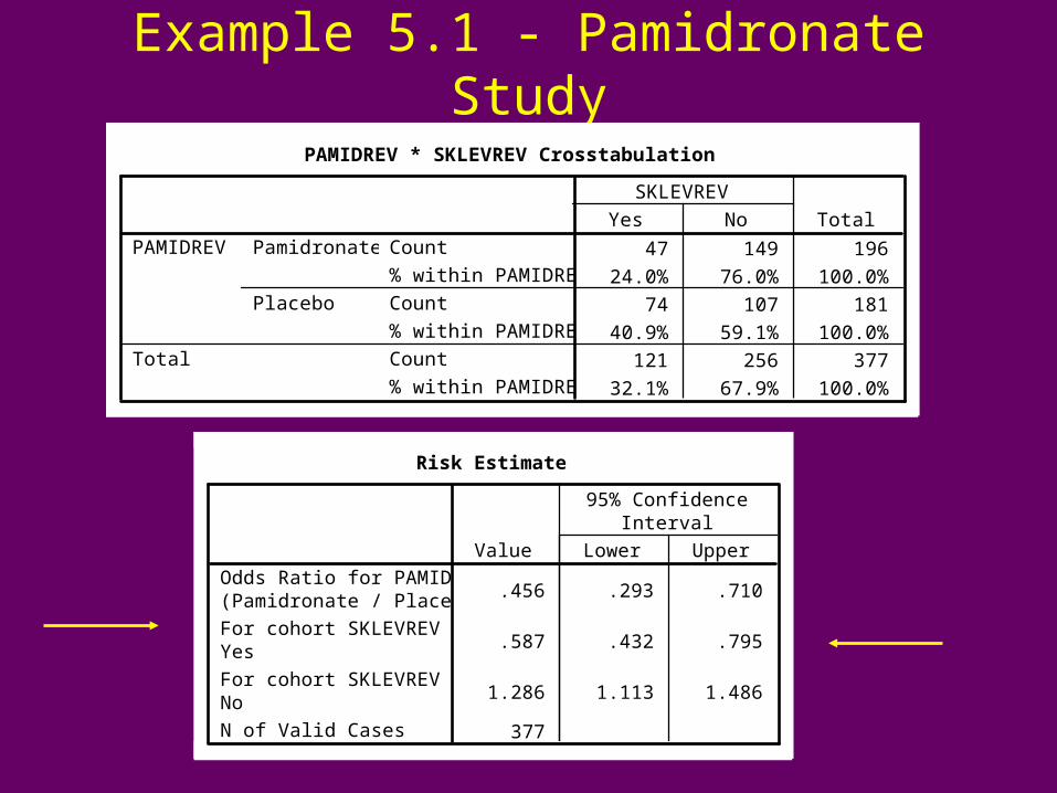
Example 5.1 - Pamidronate Study
PAMIDREV * SKLEVREV Crosstabulation
47 149 196
24.0% 76.0% 100.0%
74 107 181
40.9% 59.1% 100.0%
121 256 377
32.1% 67.9% 100.0%
Count
% within PAMIDREV
Count
% within PAMIDREV
Count
% within PAMIDREV
Pamidronate
Placebo
PAMIDREV
Total
Yes No
SKLEVREV
Total
Risk Estimate
.456 .293 .710
.587 .432 .795
1.286 1.113 1.486
377
Odds Ratio for PAMIDREV(Pamidronate / Placebo)
For cohort SKLEVREV =Yes
For cohort SKLEVREV =No
N of Valid Cases
Value Lower Upper
95% ConfidenceInterval

Example 5.2 - Lip CancerPIPESREV * LIPCREV Crosstabulation
339 149 488
69.5% 30.5% 100.0%
198 351 549
36.1% 63.9% 100.0%
537 500 1037
51.8% 48.2% 100.0%
Count
% within PIPESREV
Count
% within PIPESREV
Count
% within PIPESREV
Yes
No
PIPESREV
Total
Yes No
LIPCREV
Total
Risk Estimate
4.033 3.111 5.229
1.926 1.698 2.185
.478 .412 .554
1037
Odds Ratio forPIPESREV (Yes / No)
For cohort LIPCREV =Yes
For cohort LIPCREV = No
N of Valid Cases
Value Lower Upper
95% ConfidenceInterval
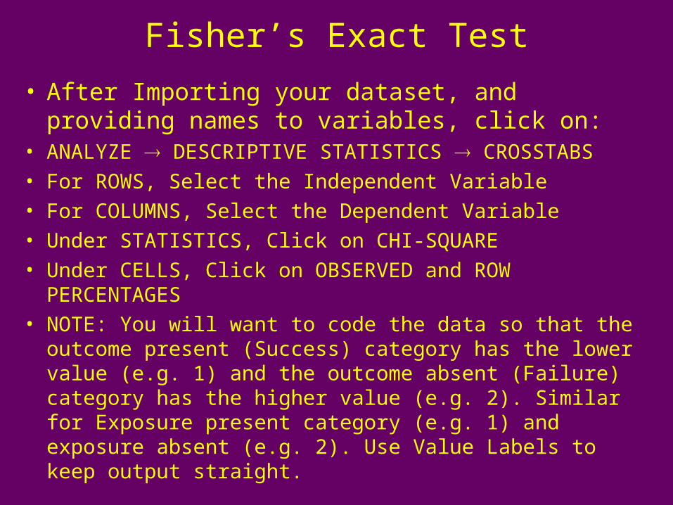
Fisher’s Exact Test
• After Importing your dataset, and providing names to variables, click on:
• ANALYZE DESCRIPTIVE STATISTICS CROSSTABS
• For ROWS, Select the Independent Variable
• For COLUMNS, Select the Dependent Variable
• Under STATISTICS, Click on CHI-SQUARE
• Under CELLS, Click on OBSERVED and ROW PERCENTAGES
• NOTE: You will want to code the data so that the outcome present (Success) category has the lower value (e.g. 1) and the outcome absent (Failure) category has the higher value (e.g. 2). Similar for Exposure present category (e.g. 1) and exposure absent (e.g. 2). Use Value Labels to keep output straight.

Example 5.5 - Antiseptic ExperimentTRTREV * DEATHREV Crosstabulation
6 34 40
15.0% 85.0% 100.0%
16 19 35
45.7% 54.3% 100.0%
22 53 75
29.3% 70.7% 100.0%
Count
% within TRTREV
Count
% within TRTREV
Count
% within TRTREV
Antiseptic
Control
TRTREV
Total
Death No Death
DEATHREV
Total
Chi-Square Tests
8.495b 1 .004
7.078 1 .008
8.687 1 .003
.005 .004
8.382 1 .004
75
Pearson Chi-Square
Continuity Correctiona
Likelihood Ratio
Fisher's Exact Test
Linear-by-LinearAssociation
N of Valid Cases
Value dfAsymp. Sig.
(2-sided)Exact Sig.(2-sided)
Exact Sig.(1-sided)
Computed only for a 2x2 tablea.
0 cells (.0%) have expected count less than 5. The minimum expected count is10.27.
b.
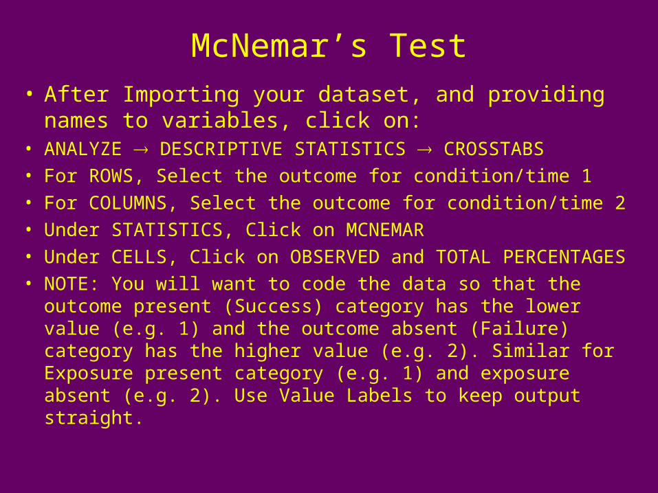
McNemar’s Test
• After Importing your dataset, and providing names to variables, click on:
• ANALYZE DESCRIPTIVE STATISTICS CROSSTABS
• For ROWS, Select the outcome for condition/time 1
• For COLUMNS, Select the outcome for condition/time 2
• Under STATISTICS, Click on MCNEMAR
• Under CELLS, Click on OBSERVED and TOTAL PERCENTAGES
• NOTE: You will want to code the data so that the outcome present (Success) category has the lower value (e.g. 1) and the outcome absent (Failure) category has the higher value (e.g. 2). Similar for Exposure present category (e.g. 1) and exposure absent (e.g. 2). Use Value Labels to keep output straight.

Example 5.6 - Report of Implant Leak
SELFREV * SURGREV Crosstabulation
69 28 97
41.8% 17.0% 58.8%
5 63 68
3.0% 38.2% 41.2%
74 91 165
44.8% 55.2% 100.0%
Count
% of Total
Count
% of Total
Count
% of Total
Present
Absent
SELFREV
Total
Present Absent
SURGREV
Total
Chi-Square Tests
.000a
165
McNemar Test
N of Valid Cases
ValueExact Sig.(2-sided)
Binomial distribution used.a.
P-value

Cochran Mantel-Haenszel Test
• After Importing your dataset, and providing names to variables, click on:
• ANALYZE DESCRIPTIVE STATISTICS CROSSTABS
• For ROWS, Select the Independent Variable
• For COLUMNS, Select the Dependent Variable
• For LAYERS, Select the Strata Variable
• Under STATISTICS, Click on COCHRAN’S AND MANTEL-HAENSZEL STATISTICS
• NOTE: You will want to code the data so that the outcome present (Success) category has the lower value (e.g. 1) and the outcome absent (Failure) category has the higher value (e.g. 2). Similar for Exposure present category (e.g. 1) and exposure absent (e.g. 2). Use Value Labels to keep output straight.
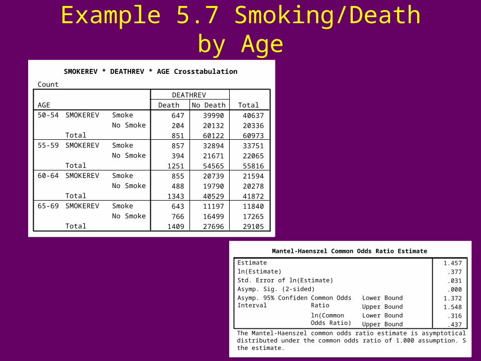
Example 5.7 Smoking/Death by Age
SMOKEREV * DEATHREV * AGE Crosstabulation
Count
647 39990 40637
204 20132 20336
851 60122 60973
857 32894 33751
394 21671 22065
1251 54565 55816
855 20739 21594
488 19790 20278
1343 40529 41872
643 11197 11840
766 16499 17265
1409 27696 29105
Smoke
No Smoke
SMOKEREV
Total
Smoke
No Smoke
SMOKEREV
Total
Smoke
No Smoke
SMOKEREV
Total
Smoke
No Smoke
SMOKEREV
Total
AGE50-54
55-59
60-64
65-69
Death No Death
DEATHREV
Total
Mantel-Haenszel Common Odds Ratio Estimate
1.457
.377
.031
.000
1.372
1.548
.316
.437
Estimate
ln(Estimate)
Std. Error of ln(Estimate)
Asymp. Sig. (2-sided)
Lower Bound
Upper Bound
Common OddsRatio
Lower Bound
Upper Bound
ln(CommonOdds Ratio)
Asymp. 95% ConfidenceInterval
The Mantel-Haenszel common odds ratio estimate is asymptotically normallydistributed under the common odds ratio of 1.000 assumption. So is the natural log ofthe estimate.
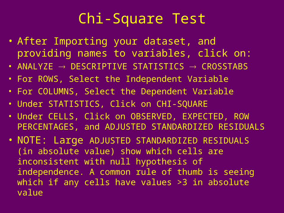
Chi-Square Test
• After Importing your dataset, and providing names to variables, click on:
• ANALYZE DESCRIPTIVE STATISTICS CROSSTABS
• For ROWS, Select the Independent Variable
• For COLUMNS, Select the Dependent Variable
• Under STATISTICS, Click on CHI-SQUARE
• Under CELLS, Click on OBSERVED, EXPECTED, ROW PERCENTAGES, and ADJUSTED STANDARDIZED RESIDUALS
• NOTE: Large ADJUSTED STANDARDIZED RESIDUALS (in absolute value) show which cells are inconsistent with null hypothesis of independence. A common rule of thumb is seeing which if any cells have values >3 in absolute value
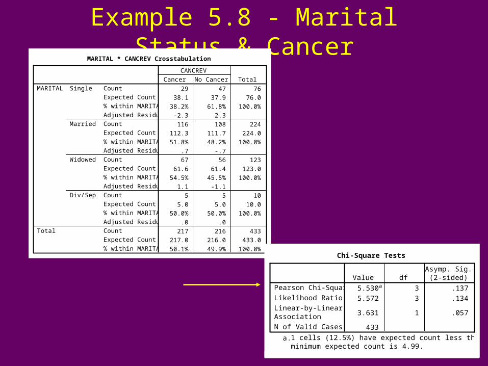
Example 5.8 - Marital Status & CancerMARITAL * CANCREV Crosstabulation
29 47 76
38.1 37.9 76.0
38.2% 61.8% 100.0%
-2.3 2.3
116 108 224
112.3 111.7 224.0
51.8% 48.2% 100.0%
.7 -.7
67 56 123
61.6 61.4 123.0
54.5% 45.5% 100.0%
1.1 -1.1
5 5 10
5.0 5.0 10.0
50.0% 50.0% 100.0%
.0 .0
217 216 433
217.0 216.0 433.0
50.1% 49.9% 100.0%
Count
Expected Count
% within MARITAL
Adjusted Residual
Count
Expected Count
% within MARITAL
Adjusted Residual
Count
Expected Count
% within MARITAL
Adjusted Residual
Count
Expected Count
% within MARITAL
Adjusted Residual
Count
Expected Count
% within MARITAL
Single
Married
Widowed
Div/Sep
MARITAL
Total
Cancer No Cancer
CANCREV
Total
Chi-Square Tests
5.530a 3 .137
5.572 3 .134
3.631 1 .057
433
Pearson Chi-Square
Likelihood Ratio
Linear-by-LinearAssociation
N of Valid Cases
Value dfAsymp. Sig.
(2-sided)
1 cells (12.5%) have expected count less than 5. Theminimum expected count is 4.99.
a.

Goodman & Kruskal’s / Kendall’s b
• After Importing your dataset, and providing names to variables, click on:
• ANALYZE DESCRIPTIVE STATISTICS CROSSTABS
• For ROWS, Select the Independent Variable
• For COLUMNS, Select the Dependent Variable
• Under STATISTICS, Click on GAMMA and KENDALL’S b
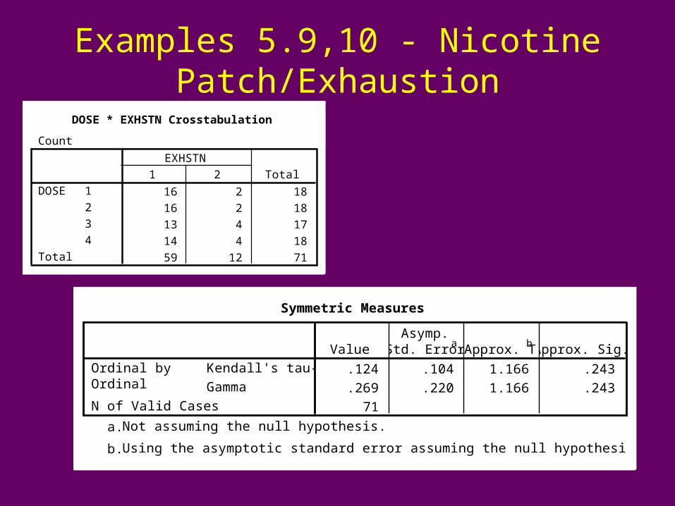
Examples 5.9,10 - Nicotine Patch/Exhaustion
DOSE * EXHSTN Crosstabulation
Count
16 2 18
16 2 18
13 4 17
14 4 18
59 12 71
1
2
3
4
DOSE
Total
1 2
EXHSTN
Total
Symmetric Measures
.124 .104 1.166 .243
.269 .220 1.166 .243
71
Kendall's tau-b
Gamma
Ordinal byOrdinal
N of Valid Cases
ValueAsymp.
Std. Errora
Approx. Tb
Approx. Sig.
Not assuming the null hypothesis.a.
Using the asymptotic standard error assuming the null hypothesis.b.

Kruskal-Wallis Test
• After Importing your dataset, and providing names to variables, click on:
• ANALYZE NONPARAMETRIC TESTS k INDEPENDENT SAMPLES
• For TEST VARIABLE, Select Dependent Variable
• For GROUPING VARIABLE, Select Independent Variable, then define range of levels of variable (Minimum and Maximum)
• Click on KRUSKAL-WALLIS H
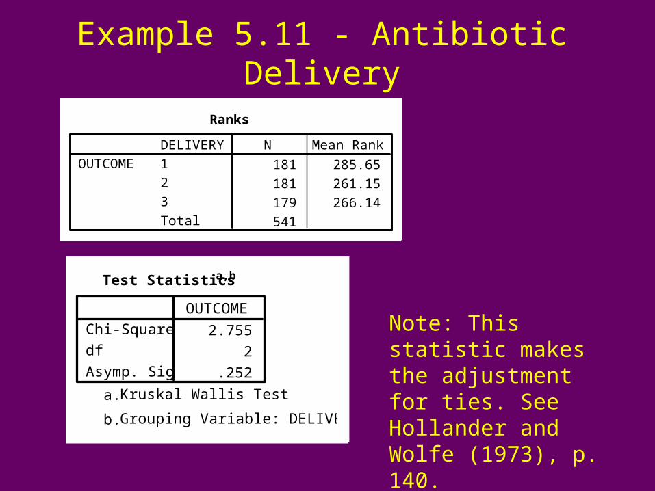
Example 5.11 - Antibiotic Delivery
Ranks
181 285.65
181 261.15
179 266.14
541
DELIVERY1
2
3
Total
OUTCOMEN Mean Rank
Test Statisticsa,b
2.755
2
.252
Chi-Square
df
Asymp. Sig.
OUTCOME
Kruskal Wallis Testa.
Grouping Variable: DELIVERYb.
Note: This statistic makes the adjustment for ties. See Hollander and Wolfe (1973), p. 140.

Cohen’s
• After Importing your dataset, and providing names to variables, click on:
• ANALYZE DESCRIPTIVE STATISTICS CROSSTABS
• For ROWS, Select Rater 1
• For COLUMNS, Select Rater 2
• Under STATISTICS, Click on KAPPA
• Under CELLS, Click on TOTAL Percentages to get the observed percentages in each cell (the first number under observed count in Table 5.17).

Example 5.12 - Siskel & EbertSISKEL * EBERT Crosstabulation
24 8 13 45
15.0% 5.0% 8.1% 28.1%
8 13 11 32
5.0% 8.1% 6.9% 20.0%
10 9 64 83
6.3% 5.6% 40.0% 51.9%
42 30 88 160
26.3% 18.8% 55.0% 100.0%
Count
% of Total
Count
% of Total
Count
% of Total
Count
% of Total
-1
0
1
SISKEL
Total
-1 0 1
EBERT
Total
Symmetric Measures
.389 .060 6.731 .000
160
KappaMeasure of Agreement
N of Valid Cases
ValueAsymp.
Std. Errora
Approx. Tb
Approx. Sig.
Not assuming the null hypothesis.a.
Using the asymptotic standard error assuming the null hypothesis.b.
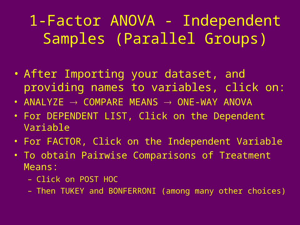
1-Factor ANOVA - Independent Samples (Parallel Groups)
• After Importing your dataset, and providing names to variables, click on:
• ANALYZE COMPARE MEANS ONE-WAY ANOVA
• For DEPENDENT LIST, Click on the Dependent Variable
• For FACTOR, Click on the Independent Variable
• To obtain Pairwise Comparisons of Treatment Means:– Click on POST HOC
– Then TUKEY and BONFERRONI (among many other choices)
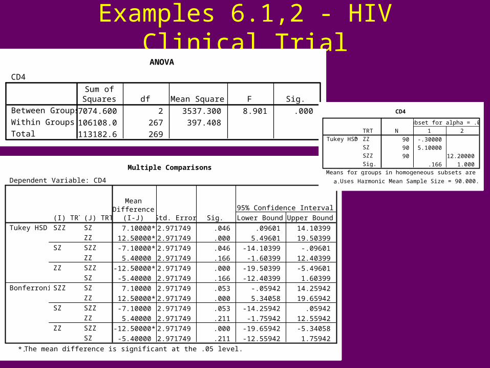
Examples 6.1,2 - HIV Clinical TrialANOVA
CD4
7074.600 2 3537.300 8.901 .000
106108.0 267 397.408
113182.6 269
Between Groups
Within Groups
Total
Sum ofSquares df Mean Square F Sig.
Multiple Comparisons
Dependent Variable: CD4
7.10000* 2.971749 .046 .09601 14.10399
12.50000* 2.971749 .000 5.49601 19.50399
-7.10000* 2.971749 .046 -14.10399 -.09601
5.40000 2.971749 .166 -1.60399 12.40399
-12.50000* 2.971749 .000 -19.50399 -5.49601
-5.40000 2.971749 .166 -12.40399 1.60399
7.10000 2.971749 .053 -.05942 14.25942
12.50000* 2.971749 .000 5.34058 19.65942
-7.10000 2.971749 .053 -14.25942 .05942
5.40000 2.971749 .211 -1.75942 12.55942
-12.50000* 2.971749 .000 -19.65942 -5.34058
-5.40000 2.971749 .211 -12.55942 1.75942
(J) TRTSZ
ZZ
SZZ
ZZ
SZZ
SZ
SZ
ZZ
SZZ
ZZ
SZZ
SZ
(I) TRTSZZ
SZ
ZZ
SZZ
SZ
ZZ
Tukey HSD
Bonferroni
MeanDifference
(I-J) Std. Error Sig. Lower Bound Upper Bound
95% Confidence Interval
The mean difference is significant at the .05 level.*.
CD4
90 -.30000
90 5.10000
90 12.20000
.166 1.000
TRTZZ
SZ
SZZ
Sig.
Tukey HSDaN 1 2
Subset for alpha = .05
Means for groups in homogeneous subsets are displayed.
Uses Harmonic Mean Sample Size = 90.000.a.

Kruskal-Wallis Test
• After Importing your dataset, and providing names to variables, click on:
• ANALYZE NONPARAMETRIC TESTS k INDEPENDENT SAMPLES
• For TEST VARIABLE, Select Dependent Variable
• For GROUPING VARIABLE, Select Independent Variable, then define range of levels of variable (Minimum and Maximum)
• Click on KRUSKAL-WALLIS H

Example 6.2(a) - Thalidomide and HIV-1
Ranks
8 24.44
8 21.63
8 6.56
8 13.38
32
TRT1
2
3
4
Total
WTGAINN Mean Rank
Test Statisticsa,b
18.070
3
.000
Chi-Square
df
Asymp. Sig.
WTGAIN
Kruskal Wallis Testa.
Grouping Variable: TRTb.
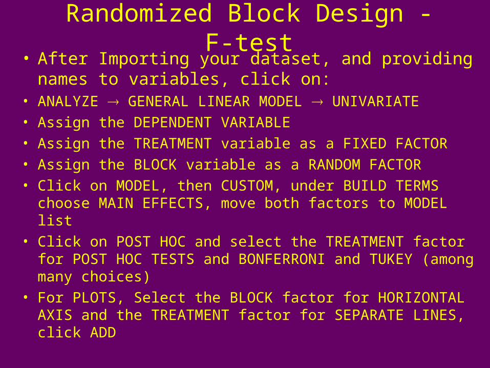
Randomized Block Design - F-test• After Importing your dataset, and providing names to
variables, click on:• ANALYZE GENERAL LINEAR MODEL UNIVARIATE
• Assign the DEPENDENT VARIABLE
• Assign the TREATMENT variable as a FIXED FACTOR
• Assign the BLOCK variable as a RANDOM FACTOR
• Click on MODEL, then CUSTOM, under BUILD TERMS choose MAIN EFFECTS, move both factors to MODEL list
• Click on POST HOC and select the TREATMENT factor for POST HOC TESTS and BONFERRONI and TUKEY (among many choices)
• For PLOTS, Select the BLOCK factor for HORIZONTAL AXIS and the TREATMENT factor for SEPARATE LINES, click ADD
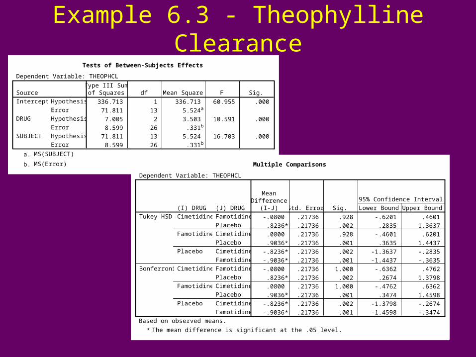
Example 6.3 - Theophylline ClearanceTests of Between-Subjects Effects
Dependent Variable: THEOPHCL
336.713 1 336.713 60.955 .000
71.811 13 5.524a
7.005 2 3.503 10.591 .000
8.599 26 .331b
71.811 13 5.524 16.703 .000
8.599 26 .331b
SourceHypothesis
Error
Intercept
Hypothesis
Error
DRUG
Hypothesis
Error
SUBJECT
Type III Sumof Squares df Mean Square F Sig.
MS(SUBJECT)a.
MS(Error)b. Multiple Comparisons
Dependent Variable: THEOPHCL
-.0800 .21736 .928 -.6201 .4601
.8236* .21736 .002 .2835 1.3637
.0800 .21736 .928 -.4601 .6201
.9036* .21736 .001 .3635 1.4437
-.8236* .21736 .002 -1.3637 -.2835
-.9036* .21736 .001 -1.4437 -.3635
-.0800 .21736 1.000 -.6362 .4762
.8236* .21736 .002 .2674 1.3798
.0800 .21736 1.000 -.4762 .6362
.9036* .21736 .001 .3474 1.4598
-.8236* .21736 .002 -1.3798 -.2674
-.9036* .21736 .001 -1.4598 -.3474
(J) DRUGFamotidine
Placebo
Cimetidine
Placebo
Cimetidine
Famotidine
Famotidine
Placebo
Cimetidine
Placebo
Cimetidine
Famotidine
(I) DRUGCimetidine
Famotidine
Placebo
Cimetidine
Famotidine
Placebo
Tukey HSD
Bonferroni
MeanDifference
(I-J) Std. Error Sig. Lower Bound Upper Bound
95% Confidence Interval
Based on observed means.
The mean difference is significant at the .05 level.*.
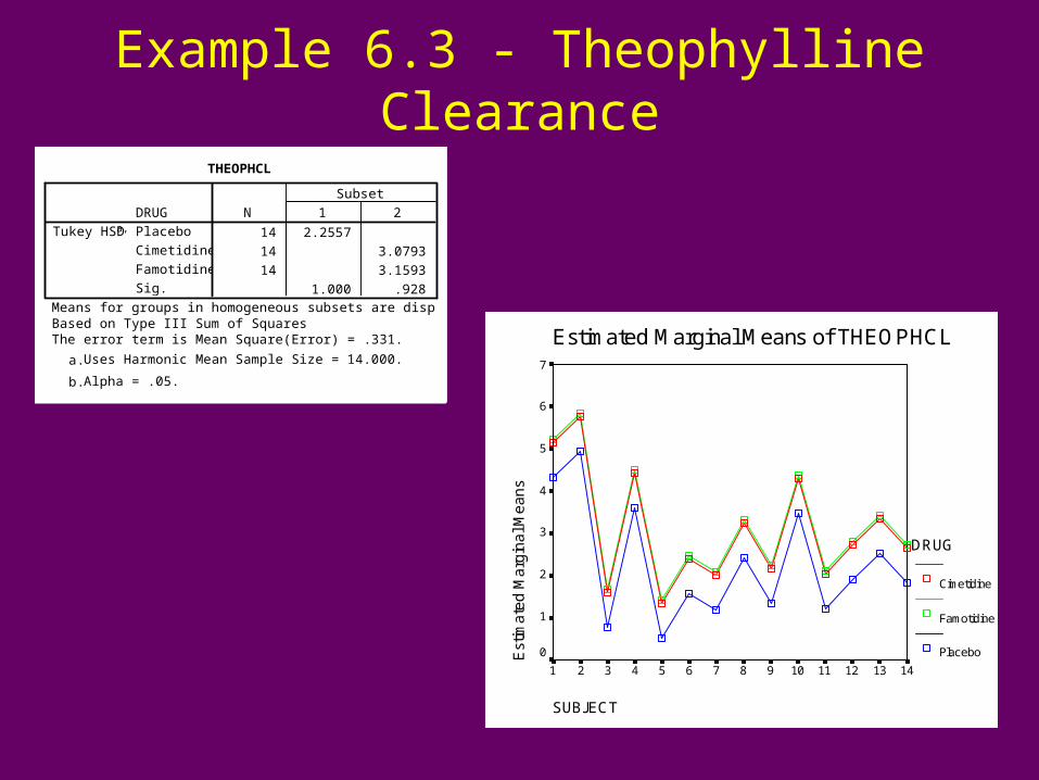
Example 6.3 - Theophylline Clearance
THEOPHCL
14 2.2557
14 3.0793
14 3.1593
1.000 .928
DRUGPlacebo
Cimetidine
Famotidine
Sig.
Tukey HSDa,bN 1 2
Subset
Means for groups in homogeneous subsets are displayed.Based on Type III Sum of SquaresThe error term is Mean Square(Error) = .331.
Uses Harmonic Mean Sample Size = 14.000.a.
Alpha = .05.b.
Estimated Marginal Means of THEOPHCL
SUBJECT
1413121110987654321
Est
ima
ted
Ma
rgin
al M
ea
ns
7
6
5
4
3
2
1
0
DRUG
Cimetidine
Famotidine
Placebo
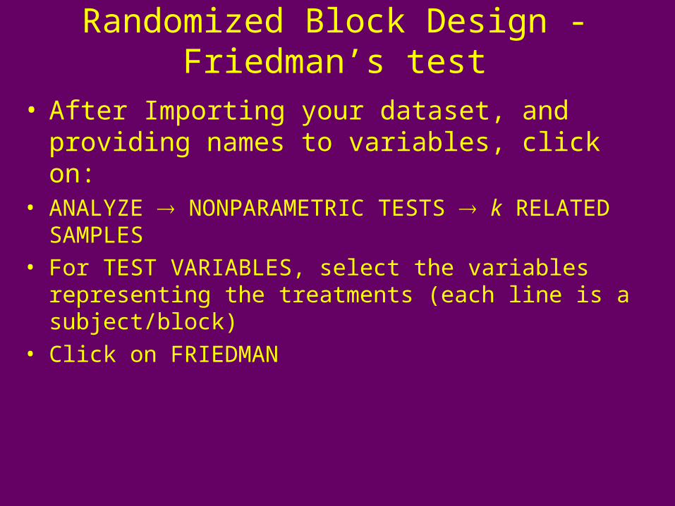
Randomized Block Design - Friedman’s test
• After Importing your dataset, and providing names to variables, click on:
• ANALYZE NONPARAMETRIC TESTS k RELATED SAMPLES
• For TEST VARIABLES, select the variables representing the treatments (each line is a subject/block)
• Click on FRIEDMAN
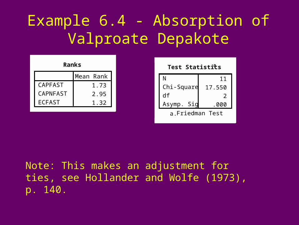
Example 6.4 - Absorption of Valproate Depakote
Ranks
1.73
2.95
1.32
CAPFAST
CAPNFAST
ECFAST
Mean Rank
Test Statisticsa
11
17.550
2
.000
N
Chi-Square
df
Asymp. Sig.
Friedman Testa.
Note: This makes an adjustment for ties, see Hollander and Wolfe (1973), p. 140.
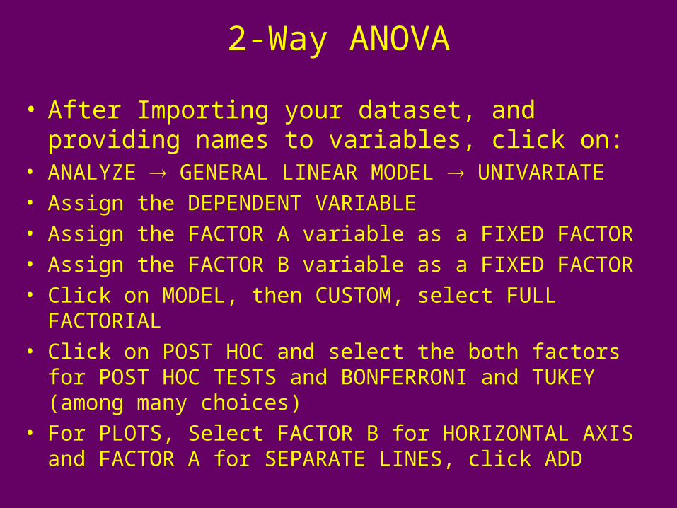
2-Way ANOVA
• After Importing your dataset, and providing names to variables, click on:
• ANALYZE GENERAL LINEAR MODEL UNIVARIATE
• Assign the DEPENDENT VARIABLE
• Assign the FACTOR A variable as a FIXED FACTOR
• Assign the FACTOR B variable as a FIXED FACTOR
• Click on MODEL, then CUSTOM, select FULL FACTORIAL
• Click on POST HOC and select the both factors for POST HOC TESTS and BONFERRONI and TUKEY (among many choices)
• For PLOTS, Select FACTOR B for HORIZONTAL AXIS and FACTOR A for SEPARATE LINES, click ADD
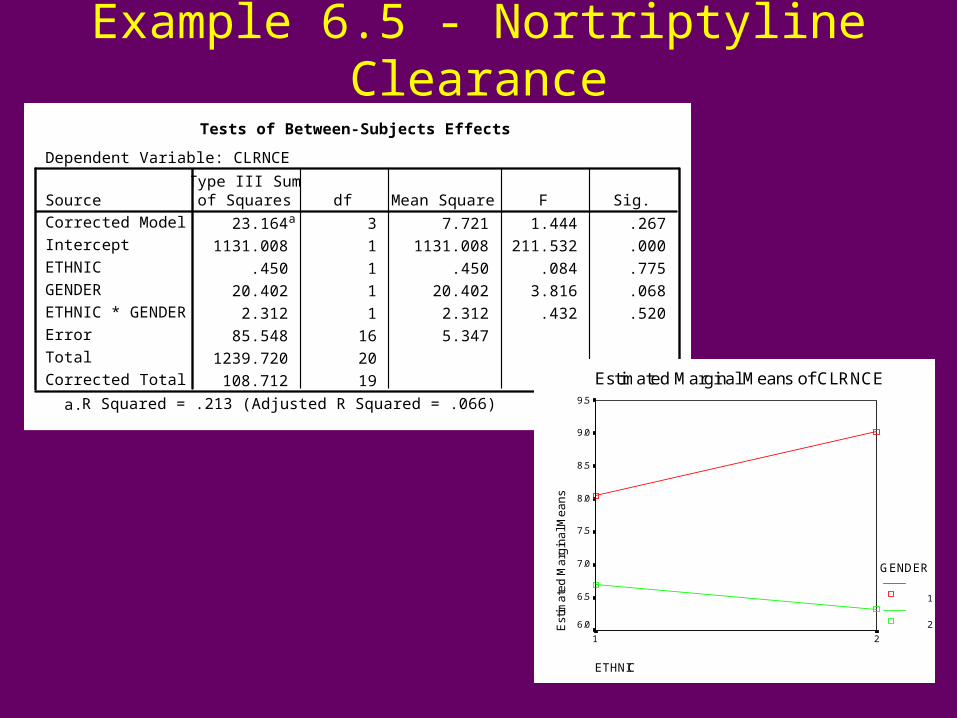
Example 6.5 - Nortriptyline ClearanceTests of Between-Subjects Effects
Dependent Variable: CLRNCE
23.164a 3 7.721 1.444 .267
1131.008 1 1131.008 211.532 .000
.450 1 .450 .084 .775
20.402 1 20.402 3.816 .068
2.312 1 2.312 .432 .520
85.548 16 5.347
1239.720 20
108.712 19
SourceCorrected Model
Intercept
ETHNIC
GENDER
ETHNIC * GENDER
Error
Total
Corrected Total
Type III Sumof Squares df Mean Square F Sig.
R Squared = .213 (Adjusted R Squared = .066)a.
Estimated Marginal Means of CLRNCE
ETHNIC
21
Est
ima
ted
Ma
rgin
al M
ea
ns
9.5
9.0
8.5
8.0
7.5
7.0
6.5
6.0
GENDER
1
2

Linear Regression
• After Importing your dataset, and providing names to variables, click on:
• ANALYZE REGRESSION LINEAR
• Select the DEPENDENT VARIABLE
• Select the INDEPENDENT VARAIABLE(S)
• Click on STATISTICS, then ESTIMATES, CONFIDENCE INTERVALS, MODEL FIT
• For histogram of residuals, click on PLOTS, and HISTOGRAM under STANDARDIZED RESIDUAL PLOTS

Examples 7.1-7.6 - Gemfibrozil ClearanceCoefficientsa
460.828 54.338 8.481 .000 345.010 576.646
-3.215 1.181 -.575 -2.723 .016 -5.732 -.698
(Constant)
CLCR
Model1
B Std. Error
UnstandardizedCoefficients
Beta
StandardizedCoefficients
t Sig. Lower Bound Upper Bound
95% Confidence Interval for B
Dependent Variable: CLGMa.
Regression Standardized Residual
1.501.00.500.00-.50-1.00-1.50
Histogram
Dependent Variable: CLGM
Fre
qu
en
cy
6
5
4
3
2
1
0
Std. Dev = .97
Mean = 0.00
N = 17.00
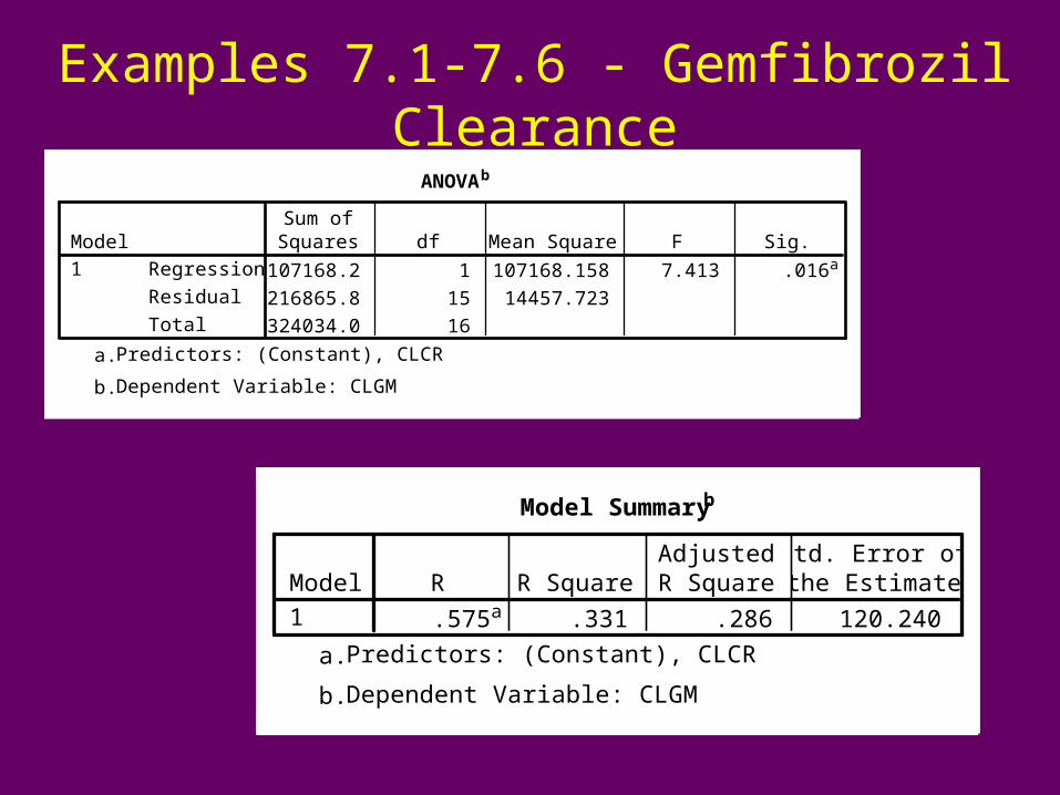
Examples 7.1-7.6 - Gemfibrozil ClearanceANOVAb
107168.2 1 107168.158 7.413 .016a
216865.8 15 14457.723
324034.0 16
Regression
Residual
Total
Model1
Sum ofSquares df Mean Square F Sig.
Predictors: (Constant), CLCRa.
Dependent Variable: CLGMb.
Model Summaryb
.575a .331 .286 120.240Model1
R R SquareAdjustedR Square
Std. Error ofthe Estimate
Predictors: (Constant), CLCRa.
Dependent Variable: CLGMb.
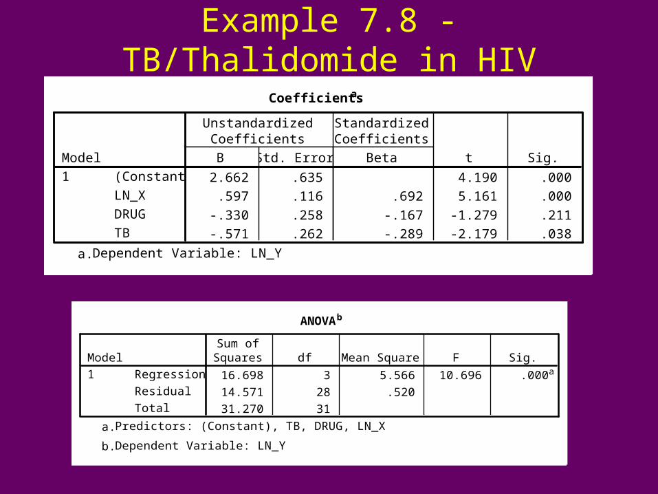
Example 7.8 - TB/Thalidomide in HIV
Coefficientsa
2.662 .635 4.190 .000
.597 .116 .692 5.161 .000
-.330 .258 -.167 -1.279 .211
-.571 .262 -.289 -2.179 .038
(Constant)
LN_X
DRUG
TB
Model1
B Std. Error
UnstandardizedCoefficients
Beta
StandardizedCoefficients
t Sig.
Dependent Variable: LN_Ya.
ANOVAb
16.698 3 5.566 10.696 .000a
14.571 28 .520
31.270 31
Regression
Residual
Total
Model1
Sum ofSquares df Mean Square F Sig.
Predictors: (Constant), TB, DRUG, LN_Xa.
Dependent Variable: LN_Yb.

Useful Regression Plots
• Scatterplot with Fitted (Least Squares) Line– GRAPHS INTERACTIVE SCATTERPLOT
– Select DEPENDENT VARIABLE for UP/DOWN AXIS
– Select INDEPENDENT VARIABLE for RIGHT/LEFT AXIS
– Click on FIT Tab, then REGRESSION for METHOD
– NOTE: Be certain both variables are SCALE in VARIABLE VIEW under MEASURE
• Partial Regression Plots (Multiple Regression) to observe association of each Independent Variable with Y, controlling for all others– Fit REGRESSION model with all Independent Variables
– Click PLOTS, then PRODUCE ALL PARTIAL PLOTS
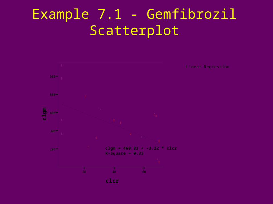
Example 7.1 - Gemfibrozil Scatterplot
Linear Regression
20 40 60
clcr
200
300
400
500
600
clg
m
clgm = 460.83 + -3.22 * clcrR-Square = 0.33
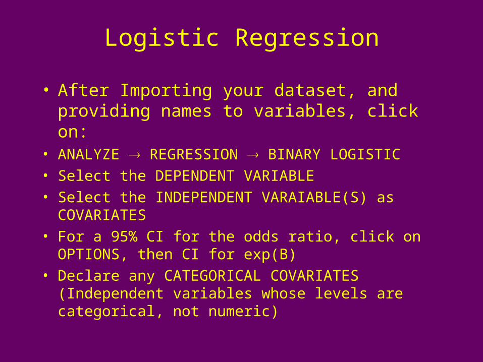
Logistic Regression
• After Importing your dataset, and providing names to variables, click on:
• ANALYZE REGRESSION BINARY LOGISTIC
• Select the DEPENDENT VARIABLE
• Select the INDEPENDENT VARAIABLE(S) as COVARIATES
• For a 95% CI for the odds ratio, click on OPTIONS, then CI for exp(B)
• Declare any CATEGORICAL COVARIATES (Independent variables whose levels are categorical, not numeric)

Example 8.1 - Navelbine Toxicity
Variables in the Equation
.488 .052 88.238 1 .000 1.628 1.471 1.803
-6.381 .690 85.498 1 .000 .002
DOSE
Constant
Step1
a
B S.E. Wald df Sig. Exp(B) Lower Upper
95.0% C.I.for EXP(B)
Variable(s) entered on step 1: DOSE.a.
Omnibus Tests of Model Coefficients
210.310 1 .000
210.310 1 .000
210.310 1 .000
Step
Block
Model
Step 1Chi-square df Sig.
Omnibus test for all regression coefficients (like F in linear regression)

Example 8.2 - CHD, BP, Cholesterol
Variables in the Equation
6.394 1.475 18.792 1 .000 598.277 33.218 10775.391
3.454 .838 17.008 1 .000 31.631 6.126 163.319
-24.020 3.699 42.158 1 .000 .000
LOG10SC
LOG10BP
Constant
Step1
a
B S.E. Wald df Sig. Exp(B) Lower Upper
95.0% C.I.for EXP(B)
Variable(s) entered on step 1: LOG10SC, LOG10BP.a.
Omnibus Tests of Model Coefficients
42.566 2 .000
42.566 2 .000
42.566 2 .000
Step
Block
Model
Step 1Chi-square df Sig.

Nonlinear Regression
• After Importing your dataset, and providing names to variables, click on:
• ANALYZE REGRESSION NONLINEAR
• Select the DEPENDENT VARIABLE
• Define the MODEL EXPRESSION as a function of the INDEPENDENT VARIABLE(s) and unknown PARAMETERS
• Define the PARAMETERS and give them STARTING VALUES (this may take several attempts)
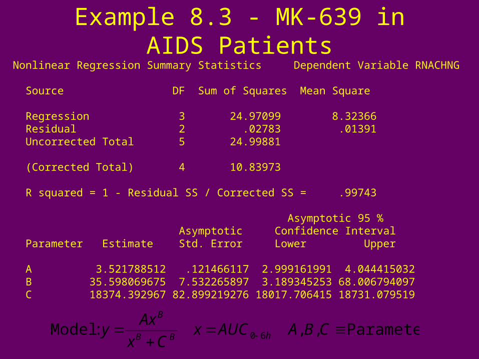
Example 8.3 - MK-639 in AIDS PatientsNonlinear Regression Summary Statistics Dependent Variable RNACHNG
Source DF Sum of Squares Mean Square
Regression 3 24.97099 8.32366 Residual 2 .02783 .01391 Uncorrected Total 5 24.99881
(Corrected Total) 4 10.83973
R squared = 1 - Residual SS / Corrected SS = .99743
Asymptotic 95 % Asymptotic Confidence Interval Parameter Estimate Std. Error Lower Upper
A 3.521788512 .121466117 2.999161991 4.044415032 B 35.598069675 7.532265897 3.189345253 68.006794097 C 18374.392967 82.899219276 18017.706415 18731.079519
Parameters,, :Model 60
CBAAUCxCx
Axy hBB
B
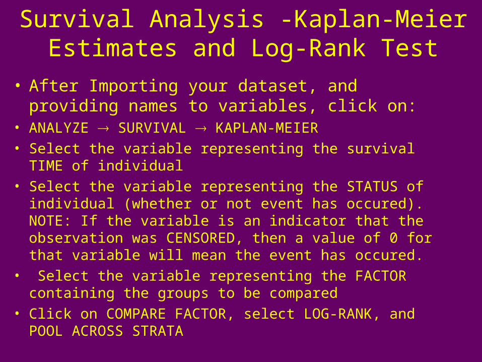
Survival Analysis -Kaplan-Meier Estimates and Log-Rank Test
• After Importing your dataset, and providing names to variables, click on:
• ANALYZE SURVIVAL KAPLAN-MEIER
• Select the variable representing the survival TIME of individual
• Select the variable representing the STATUS of individual (whether or not event has occured). NOTE: If the variable is an indicator that the observation was CENSORED, then a value of 0 for that variable will mean the event has occured.
• Select the variable representing the FACTOR containing the groups to be compared
• Click on COMPARE FACTOR, select LOG-RANK, and POOL ACROSS STRATA

Examples 9.1-2 - Navelbine and Taxol in MiceSurvival Analysis for TIME
Factor REGIMEN = 1
Time Status Cumulative Standard Cumulative Number Survival Error Events Remaining
6 0 .9796 .0202 1 48 8 0 .9592 .0283 2 47 22 0 .9388 .0342 3 46 32 0 4 45 32 0 .8980 .0432 5 44 35 0 .8776 .0468 6 43 41 0 .8571 .0500 7 42 46 0 .8367 .0528 8 41 54 0 .8163 .0553 9 40
Factor REGIMEN = 2
Time Status Cumulative Standard Cumulative Number Survival Error Events Remaining
8 0 .9333 .0644 1 14 10 0 .8667 .0878 2 13 27 0 .8000 .1033 3 12 31 0 .7333 .1142 4 11 34 0 .6667 .1217 5 10 35 0 .6000 .1265 6 9 39 0 .5333 .1288 7 8 47 0 .4667 .1288 8 7 57 0 .4000 .1265 9 6

Examples 9.1-2 - Navelbine and Taxol in MiceSurvival Functions
TIME
706050403020100
Cu
m S
urv
iva
l
1.1
1.0
.9
.8
.7
.6
.5
.4
.3
REGIMEN
2
2-censored
1
1-censored
Test Statistics for Equality of Survival Distributions for REGIMEN Statistic df Significance Log Rank 10.93 1 .0009
This is the square of the Z-statistic in text, and is a chi-square statistic
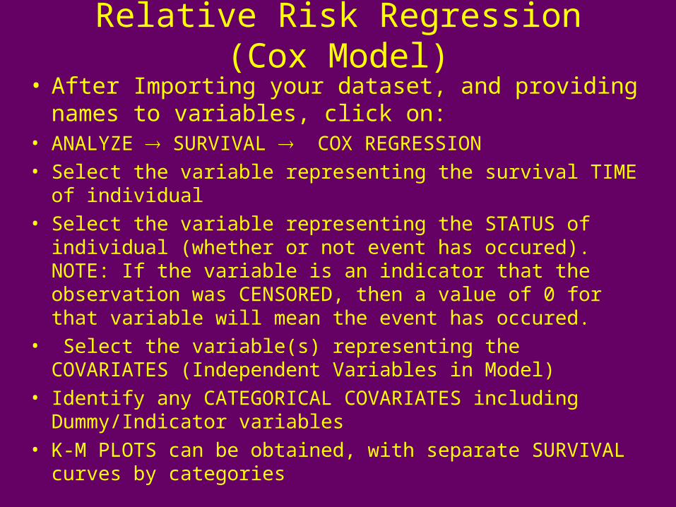
Relative Risk Regression (Cox Model)
• After Importing your dataset, and providing names to variables, click on:
• ANALYZE SURVIVAL COX REGRESSION
• Select the variable representing the survival TIME of individual
• Select the variable representing the STATUS of individual (whether or not event has occured). NOTE: If the variable is an indicator that the observation was CENSORED, then a value of 0 for that variable will mean the event has occured.
• Select the variable(s) representing the COVARIATES (Independent Variables in Model)
• Identify any CATEGORICAL COVARIATES including Dummy/Indicator variables
• K-M PLOTS can be obtained, with separate SURVIVAL curves by categories

Example 9.3 - 6MP vs Placebo
Variables in the Equation
-1.509 .410 13.578 1 .000 .221 .099 .493TRTB SE Wald df Sig. Exp(B) Lower Upper
95.0% CI for Exp(B)
Survival Function for patterns 1 - 2
REMSTIME
3020100-10
Cu
m S
urv
iva
l
1.2
1.0
.8
.6
.4
.2
0.0
TRT
Placebo
6MP
Top Related