


Languages
Pages
Legal


Spatial Econometrics Revisited: A Case Study of Land Values in Roanoke County
Ioannis K. Kaltsas European Investment Bank
100 Boulevard Konrad Adenauer
L-2940 Luxembourg Luxembourg
Email: [email protected] Tel: 352 43794662
Darrell J. Bosch Dept of Ag & Applied Econ
Virginia Tech Blacksburg, VA 24061 Email: [email protected] Phone: 540-231-5265
Anya McGuirk Dept of Ag & Applied Econ
Virginia Tech Blacksburg, VA 24061
Email: [email protected] Phone: 540-231-6301
May 2005
Paper prepared for presentation at the American Agricultural Economics Association
Annual Meeting, Providence, Rhode Island, July 24-27, 2005.
Keywords: misspecification tests, spatial autocorrelation, residential settlement, urban sprawl
JEL code: Q24
Copyright 2005 by Ioannis Kaltsas, Darrell Bosch, and Anya McGuirk. All rights reserved. Readers may make
verbatim copies of this document for noncommercial purposes by any means, provided that this copy right notice
appears on all such copies.

1
Spatial Econometrics Revisited: A Case Study of Land Values in Roanoke County
Abstract: Omitting spatial characteristics such as proximity to amenities from hedonic land
value models may lead to spatial autocorrelation and biased and inefficient estimators. A spatial
autoregressive error model can be used to model the spatial structure of errors arising from
omitted spatial effects. This paper demonstrates an alternative approach to modeling land values
based on individual and joint misspecification tests using data from Roanoke County in Virginia.
Spatial autocorrelation is found in land value models of Roanoke County. Defining
neighborhoods based on geographic and socioeconomics characteristics produces better
estimates of neighborhood effects on land values than simple distance measures. Implementing a
comprehensive set of individual and joint misspecification tests results in better correction for
misspecification errors compared to existing practices.

2
Introduction
Traditionally, economists have constructed hedonic functions to capture the relative
importance of land attributes affecting land values (Xu, Mittelhammer, and Barkley). Recent
studies emphasize a growing consensus regarding the need to incorporate spatial characteristics
such as proximity to amenities as explicit variables (Can and Megboludge; Basu and Thibodeau).
However, some spatial features may be omitted from the model (Bockstael and Bell; Irwin;
Fleming) causing the underlying error of the regression to be spatially autocorrelated. Spatial
autocorrelation due to omitted spatial features causes least squares estimators to be biased and
inefficient, making inference based on them invalid (Basu and Thibodeau). Consequently, it is
important to determine the source of autocorrelation in order to correctly specify the model.
A spatial autoregressive error model can be used to model the spatial structure of errors
arising from omitted spatial effects (Anselin 1988; Anselin and Kelejian). According to Anselin
(1988) the spatial autoregressive component corrects predicted values by an estimate of the
prediction error’s relationship to nearby observations and thus mimics the behavior of real estate
appraisers. The influence of nearby properties on land value is determined using an exogenously
determined weight matrix.
Basu and Thibodeau argue that a spatial autoregressive model may be misspecified when
the observed spatial dependence is caused by factors other than omitted variables. Sometimes
the chosen functional form does not adequately allow for heterogeneity over space, and the
estimated parameters are unstable usually varying by location. For example, most land value
models assume that the functional form is the same for both developed and vacant land parcels
(Beaton). However, developed and undeveloped land parcels may follow different stochastic
processes. Part of the observed spatial autocorrelation in the residuals may be attributed to this

3
structural instability. Anselin (1988) suggests that the problem of distinguishing the sources of
observed spatial autocorrelation is highly complex and proposes testing structural stability before
creating an autoregressive model. The assumptions of normality and heteroskedasticity should
also be tested before testing the model for spatial autocorrelation (Anselin 1988; Anselin and
Kelejian). The premise of this approach is that by first verifying the assumptions of normality,
heteroskedasticity and correct functional form, researchers may ensure that spatial dependence is
the source of autocorrelation and that incorporation of spatial structure results in correct model
specification.
Although the proposed ideas are better than past approaches of dealing with possible
spatial autocorrelation—there are still problems with how this approach is currently implemented
and, even more fundamentally, with its basic premise. To date, most spatial econometric studies
examine only a subset of the testable statistical assumptions underlying the model estimated
(Anselin 1999). The problem with this partial approach is that the statistical inferences drawn
from a model are generally only valid if all the assumptions underlying the model are valid. The
possibility of invalid inference is further exacerbated by the fact that the assumptions that are
tested are usually examined one at a time, despite the fact that most of the tests conducted are
only valid if all remaining assumptions underlying the model are correct (Spanos). For example,
most tests of parameter stability assume the right functional form is specified, the model errors
are not autocorrelated, the conditional variance is homoskedastic, etc. If any of these other
assumptions (maintained hypotheses) are not valid, incorrect inferences may be drawn, in this
example, from the parameter stability test. Alston and Chalfant illustrate just how much we can
be misled by misspecification test results when the remaining model assumptions are not valid.
Their Monte Carlo experiments show that one can incorrectly conclude that a model suffers from

4
parameter instability 100 percent of the time, when the real problem is something completely
different. Other authors have shown similar problems when testing other model assumptions
(see for example Bera and Jarque; Ghali; Lahiri and Egy; and Savin and White). The implication
of this research is that if a model does indeed suffer from spatial dependence, tests conducted to
ensure that all other assumptions are valid are likely to be unreliable. Thus, there is no way to
ensure that all the other model assumptions are correct before focusing on the autocorrelation
assumption as suggested in the literature.
McGuirk, Driscoll, and Alwang suggest a way around this circularity problem. They
suggest that all possible model assumptions need to be tested. To examine the model
assumptions, they suggest the use of both individual and joint tests. Once the battery of tests has
been conducted, they illustrate how the results should be interpreted as a group to decide the
most likely source(s) of misspecification. Basically they observe that one should never conclude
based on the results of a single test that the assumption being examined is or is not valid and they
show how the size of the respective p-values of the various tests can provide some hints
regarding the most likely source(s) of misspecification. Once the most likely source(s) of
misspecification have been identified, they suggest “fixing” the likely problem(s)--but before
concluding that the model is well-specified, the new model must be subjected to the full battery
of tests again. Only when the “fix” leads to a model that passes all misspecification tests can one
conclude that all the tested underlying assumptions are satisfied. In this approach to model
respecification, model fit (R2) plays no role in the decision process. McGuirk and Driscoll
illustrate that high fitting power does not guarantee a model’s statistical validity. Thus, while
spatial autoregressive corrections often improve model fit, the corrected model may or may not
be an improvement over the original model in terms of the relevance of the underlying statistical
5
assumptions (statistical validity). Only the results from the battery of misspecification tests on
this new model can indicate whether it is statistically valid.
The problem of determining how to respecify a model, given the results from a battery of
misspecification tests, is not necessarily straight forward if spatial autocorrelation is the main
suspect. Typically the specification of the spatial structure in spatial econometric models is
arbitrary; there are no rules to determine the spatial relationship among individual observations;
and there is no clear way to test the structural validity of the exogenously determined spatial
weight matrix. Existing non-nested tests only select the weight matrix that maximizes the fitting
power of the model. Spatial weight matrices are typically constructed using mathematically
computed distances and, thus, geographical proximity is the only criterion to account for
neighborhood effects. However, the size of neighborhoods might often be inappropriate for a
given case study and proximity might not always be the best criterion for determining
neighborhoods. In the approach advocated here and by McGuirk, Driscoll, and Alwang, the only
real test of whether the spatial autocorrelation has been modeled adequately is whether or not the
battery of misspecification tests performed on the respecified model indicate that the model
satisfies all the testable assumptions underlying the model.
The purpose of this paper is to address existing limitations of spatial modeling efforts in
the context of modeling land values and to demonstrate this alternative approach based on
individual and joint misspecification tests using data from Roanoke County in Virginia. We first
establish that there is spatial dependence in the values of land parcels in Roanoke County. Then
by implementing a comprehensive set of individual and joint misspecification tests suggested by
Spanos and McGuirk, Driscoll, and Alwang we establish a statistically sound model, which is
more reliable than models based on current spatial econometric practices.

6
Data
The data were collected as part of an interdisciplinary effort to analyze the fiscal and
environmental consequences of alternative residential development patterns using Roanoke
County, Virginia as a case study (Diplas et al.; Bosch et al.). A land value model was estimated
to help researchers and policymakers evaluate the effects of alternative residential settlement
forms on assessed land values and property tax receipts.
A random sample of observations used to estimate the model was obtained from the
Roanoke County Division of Planning and the Roanoke County Division of Tax and Assessment
data base. There were 1,844 transactions of vacant and non-vacant land parcels for the period of
1996 to 1997. Table 1 contains the descriptive statistics of variables used in estimating the land
value model. The price of the parcels reflects the value of the land alone. Prices of parcels with
structures were computed by subtracting the assessed value of the structure from the parcel’s
recorded transactions price. The sample average price per square meter is $23.13 while the
median is $3.
Parcel area varies from 0.005 hectares (a parcel close to the urban fringe of Roanoke
County) to 216 hectares (a parcel of steep and remote agricultural land). Elevation of the center
of the parcel is measured in meters above sea level. Slope is the average slope of the parcel
measured in geometric degrees. There is a high correlation (r=0.68) between the slope of the
parcel and its elevation. Most of the developed parcels are located on relatively flat land with
low elevation. The soil quality of the land parcels was classified into three categories according
to permeability. More permeable soils are associated with lower flood risk and soil erosion. The
dummy variable representing Soil Quality 1 (3% of the parcels) is the less absorbing category of
soil, while Soil Quality 2 (87% of the parcels) has an intermediate level of penetrability.
7
Point to point distances of parcels from shopping malls, the city of Roanoke and the town
of Blacksburg are measured in meters. The minimum distance of the parcels to either of two
urban centers is about 3 kilometers. However, the town centers may be less important than
shopping malls in terms of daily commuting. The Planning Department of Roanoke County
(PDRC) estimates that several thousand consumers visit the two county malls daily.
Additionally, these malls have become the center of development of hundreds of small
businesses, which offer employment to thousands of Roanoke County residents. According to the
PDRC, the development rates of the areas close to the shopping malls are expected to be the
highest in the county for the next five years.
About 5% of the parcels are located next to a major road, which may affect the land price
negatively due to noise and air pollution. More open space and easier access to natural amenities
may also be captured by the population density of the census blocks in which the parcel belongs.
The average population density of the sample is about 6 people per hectare. The dummy
variable for development indicates whether a parcel contains some type of construction (88% of
the sample) or is undeveloped (12% of the sample). The Coordinates X and Y identify the exact
location of the center of each parcel and define the proximity and neighboring effects of parcels.
Coordinate X increases in a west and northerly direction while coordinate Y increases in an east
and northerly direction. The year dummy variable indicates whether a parcel was sold in 1996
(Year=0) or in 1997 (Year=1). According to the U.S. Bureau of Census, the average price of
rural land in Roanoke County increased by 1.5% in 1997 relative to 1996.
A Statistical Model Based on Spatial Independence
The following model was created assuming that sample observations are not spatially correlated.

8
Log(Price) = A0 + A1[Log(Size)] + A2[Log(Size)]2 + A3[Log(Elevation)] + A4[Log(Elevation)]2
+ A5(Soil1) + A6(Soil2) +A7(Population) + A8(Population)2 + A9[Log(Mall)] + A10[Log(Mall)]2
+ A11[Log(Town)] + A12(Developed) + A13(Road) + A14(Year) + A15[Log(X)] + A16[Log(Y)] +
A17Log(X)Log(Y)] + u [1]
where Price is parcel price per square meter; Size is parcel area; Elevation is average parcel
elevation; Soil1 and Soil2 are dummy variables capturing soil quality; Population is the
population density in the U.S. census block containing the parcel; Mall is minimum distance to
an existing mall; Town is minimum distance to the closest town; Developed indicates whether
the parcel is vacant; Road reveals whether the parcel is adjacent to a major Road; Year shows if
the parcel was sold in 1996 or 1997; the Coordinates X and Y determine the exact location of the
parcel; and u represents the error term.
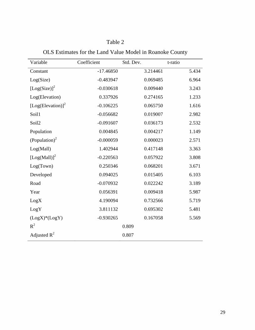
If one were to assume neither spatial autocorrelation nor any other misspecification
problems, the OLS model explains approximately 80% of the variation in the land transaction
prices (Table 2). The value of a land parcel per square meter is expected to be lower for larger
parcels. Parcels, which already have some type of residential or commercial development, have
higher transaction prices. Lower water permeability (and consequently higher flood risk) affects
parcel value negatively, while a parcel sold in 1997 has a higher value than a similar parcel sold
in 1996. A careful analysis of the non-linear relations of the model and the value range of the
variables indicates that longer distance from the closest mall as well as higher elevation and
lower population density affect land transaction prices positively but at a decreasing rate.
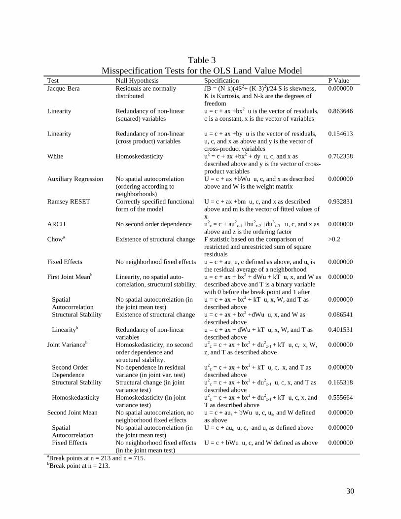
Current spatial econometric studies typically test for normality, homoskedasticity, and
structural stability. The Jacque-Bera test (Table 3) rejects the null hypothesis that the errors are
normally distributed. However, this test is very sensitive to outliers. When 2% of the extreme

9
sample observations were dropped, the hypothesis of normality was not rejected. The P-value of
the White test (Table 3) supports the hypothesis of homoskedasticity. Chow tests, conducted
after ordering the observations by neighborhoods according to the numerical code of the
Roanoke County Planning Commission, did not support the hypothesis of structural breaks at
300, 600, 900, and 1,200 observations (not shown in the table). Following the existing spatial
econometric literature (Anselin 1988), we can conclude that if we find observed spatial
autocorrelation in the econometric model then this spatial autocorrelation is the result of omitting
relevant spatial characteristics.
Testing for Spatial Independence
The sample was subdivided into neighborhoods based on the classification scheme used by the
Roanoke County Planning Commission. The criteria used for this classification are geographic
proximity of spatial units, level of economic development, and conventional and administrative
definitions of neighborhoods from other departments of the local government. The sample
contains 164 neighborhoods, and each neighborhood contains an average of 12 land parcels
included in the sample. Neighborhoods vary in size with some close to Roanoke City having a
diameter smaller than 0.3 Km, while neighborhoods at the borders of the Roanoke County are
large enough to capture similar characteristics of remote parcels. These neighborhoods were used
as spatial lags for our case study, and a weight matrix was developed with average values of land
parcels in each defined neighborhood.
Two tests were conducted of the hypothesis of no spatial autocorrelation in the land value
model. The Moran’s I test supports the existence of spatial autocorrelation. The statistic I equals
0.928 and ZI equals 5.54, which supports rejection of the hypothesis of no spatial autocorrelation
(P-value less than 0.001). The following auxiliary regression was also used:
10
u = Xb + kWu + ε [2]
where u and X are the residuals and explanatory variables of [1], b and k are the estimated
coefficients, W is the weight matrix based on the number of parcels in the neighborhood, and ε is
the error term of [2]. The null hypothesis is H0: k = 0 against H1: k ≠ 0. The F-test for H0
provides evidence against the null hypothesis (F-statistic = 17.98, P-value less than 0.001).
Consequently, both tests indicate spatial autocorrelation and that [1] is not well specified.
Correcting for Spatial Autocorrelation
While maximum likelihood techniques are often used to account for error spatial autocorrelation
(Anselin 1988) the approach becomes problematic with large datasets because of difficulties in
calculating eigenvalues of the spatial weight matrix (Pinkse and Slade; Kelejian and Prucha
1999). Alternative parametric and nonparametric estimation techniques have been proposed.
Parametric Techniques
Parametric techniques, which create an alternative autoregressive model using instrumental
variables, are simple and require limited computing capacity compared to non-parametric
techniques. Their major disadvantage is the arbitrary choice of instrumental variables. Studies
that use two or three stage least squares techniques (Land and Deane; Kelejian and Prucha, 1998)
recognize that the efficiency of their instrumental variable estimator relies on the proper choice
of the instruments. Researchers (Land and Deane; Kelejian and Robertson; Kelejian and Prucha
1998) suggest that two stage least squares (2SLS) estimators of the spatial autoregressive model
are consistent and asymptotically normal. Assume that the structure of the spatial autoregressive
model is:
Y = c W Y + X b + e [3]
and
11
W Y = k W X b + u [4]
where W is the weight matrix, c is the spatially autoregressive coefficient, WY is the spatial lag
of land prices, WX is the set of instruments and e is a vector of error terms. Anselin (1988)
proves that the spatial lag term WY is always correlated with the error term. Consequently, the
spatial lag term should be treated as an endogenous variable and proper estimation methods
should be used to account for endogeneity (OLS estimators will be biased and inconsistent due to
simultaneity error). Most spatial econometric studies (Kelejian and Prucha 1999) agree that a
theoretically sound choice of an instrument for WY would include the set of lagged independent
variables WX. According to Anselin (1999), this spatial two stage least squares estimator is
consistent and asymptotically normal, similar to the case of the standard two stage least squares
estimator in time series initially proposed by Schmidt.
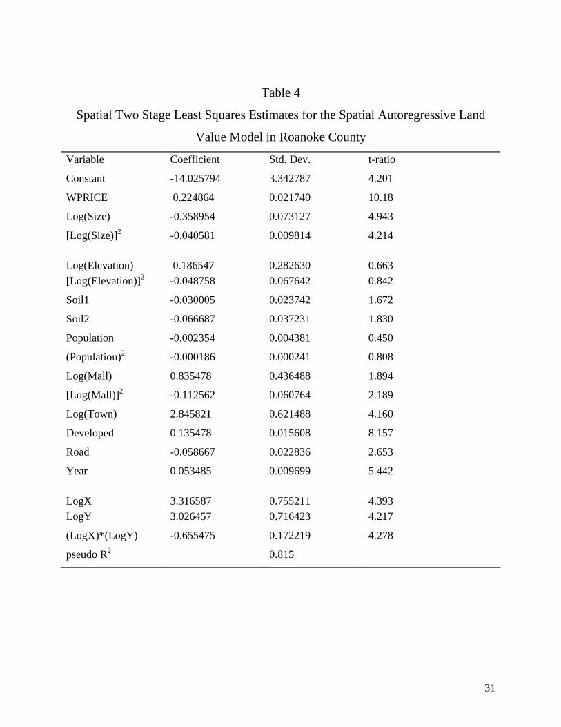
Table 4 summarizes the spatial two stage least squares estimates for the land value model
in Roanoke County. The signs and the values of almost all coefficients are similar to those of
model [1]. Larger undeveloped parcels with impermeable soil, located far from a shopping mall
and close to town center are expected to have lower transaction prices per square meter. A major
highway attached to the lot or high population density also reduces land values. Transaction
prices also increased in 1997 relative to the previous year. Finally, the positive sign of WPRICE
(average value of other parcels in the neighborhoods defined by the Roanoke County Planning
Commission) indicates the value of a parcel will increase if land values of neighboring parcels
increase. This parametric model captures spatial dependence among prices in Roanoke County
and its fitting power exceeds 81%.
However, misspecification tests imply that the two stage least squares model violates
fundamental statistical assumptions. The White test indicates that the error terms of the model

12
are not homoskedastic, despite the fact that homoskedasticity was satisfied in the initial model.
The auxiliary regression test indicates that there is no support for the assumption of no spatial
autocorrelation.
Non-Parametric Techniques
Non-parametric techniques can achieve values very close to the actual maximum
likelihood estimates faster and with less computing capacity compared to maximum likelihood
estimates (Anselin 1999; Bockstael and Bell; Kelejian and Prucha 1998). The Generalized
Moments Estimator (GME) developed by Kelejian and Prucha (1998) was estimated as part of
this study. GME is based on the three moments of the error term, u, which appears in the
formulation of the traditional error autoregressive model:
Y = X b + e [5]
and
e = c We + u [6]
Due to limitations of space, we briefly summarize the results of the estimation. The model
explains about 88% of the variation in land value prices while the signs of almost all parameter
coefficients remain the same as those in the two stage least squares model. The only exception is
that population density is statistically significant and higher population density leads to higher
land transaction prices, after evaluating linear and non-linear terms for the range of data in
Roanoke County. However, misspecification tests indicated the presence of spatial
autocorrelation, a nonnormal error distribution, and heteroscedasticity. A more complete
discussion is available in Kaltsas.
An Alternative Approach
The alternative approach to derive a statistically adequate model follows Spanos. We conducted
13
a more comprehensive set of individual and joint misspecification tests on model [1]. Then an
iterative procedure of respecification and testing led to the adoption of our final models.
Table 3 summarizes the results of a set of individual and joint misspecification tests for
the land value model [1]. Table 3 contains two tests for linearity, which indicate that non-linear
(squared and cross-product) variables are not essential for the land value model. The Ramsey
test also confirms that the functional form of the model is adequate for our data. The ARCH test
provides no support for the null hypothesis that there is no second-order spatial dependence.
Thus, the residual terms of the land value model seem to exhibit first (of the means) and second
(of the variance) order spatial dependence. The joint mean tests in Table 3 confirm that the
hypotheses of linearity, structural stability and no spatial dependence do not hold jointly.
Similarly, the joint variance test indicates the hypotheses of homoskedasticity, structural stability
and second order dependence are not supported by our data. The parcels are ordered by
neighborhood and then by development status (undeveloped parcels and then developed parcels),
while developed parcels are also ordered using the assessed value of the construction on the
parcels. Both individual and joint misspecification tests (ARCH, Chow, First Joint Mean and
Joint Variance tests) indicate that there is no support for existence of breaks in the structure of
[1]. Despite the evidence of structural stability, parameters (b and σ2) may vary across
neighborhoods as indicated by the results of both individual and joint misspecification tests
(Fixed Effects from Neighborhoods and Second Joint Mean Test) for the null hypothesis that
parameters vary across neighborhoods.
The above test results indicate that spatial autocorrelation is probably the most serious
problem in [1]. In the First Joint Mean Test for the hypotheses of linearity, no spatial
autocorrelation and structural stability, spatial autocorrelation has the lowest P-value in the joint

14
test. Similarly, second order dependence seems to be the main reason for the rejection of the
joint hypothesis in the joint variance test. At the same time the low P-values of the no
neighborhood fixed effects hypothesis and the joint hypothesis of no spatial autocorrelation and
no neighborhood fixed effects provide evidence against the hypothesis that parameters are stable
across neighborhoods (Second Joint Mean Test). In the joint mean test of no spatial
autocorrelation and no neighborhood fixed effects, rejection of both individual hypotheses leads
to rejection of the joint hypothesis.
Given that missing neighborhood specific variables are often the source of spatial
autocorrelation (Anselin 1999), a set of neighborhood dummies were added to [1]. After
estimating the fixed effects land value model to account for neighborhood effects, we retested
the model using the same set of misspecification tests. The fixed effects model accounts for
neighborhood effects by deducting from all variables their average values within each
neighborhood. Neighborhoods are those defined by the Planning Department in Roanoke
County. The resulting model showed an improvement in the P-value (Auxiliary Regression and
Joint Mean Test) of the hypothesis of no spatial autocorrelation. The P-value of the ARCH test
also improved; however, there was still significant evidence of second order dependence. The
Chow tests using the same ordering (by development status, assessed value of constructions, and
by neighborhood) indicated the existence of structural breaks. In the Joint Mean Test, we
examined the joint hypothesis of linearity, no spatial autocorrelation and structural stability. The
results indicated no support for this joint hypothesis probably due to lack of support for the
structural stability hypothesis. Similarly, lack of support for structural stability was probably the
reason for the low P-value in the joint variance test. Given the results of the joint tests, structural
instability seemed to be the major source of misspecification in the fixed effects model.
15
In the fixed effects model there was strong evidence for a structural break between
developed and undeveloped parcels. The P-value of the Chow test for n = 213 corresponding to
the vacant parcels was close to zero. Plots of recursive OLS estimates indicated substantial
change in the magnitude of coefficient estimates for several variables after the first 213
observations of the vacant parcels. Plots also indicated the possibility of structural instability in
the developed parcels when they were ordered according to the assessed value of their
construction. Almost all plots had some type of “jump” around the 750th observation, when the
assessed value of the construction was about $60 per square foot. Land parcels with expensive
construction may follow a different stochastic process than parcels with inexpensive
constructions.
In addition, window OLS (estimating the value of coefficients for observations 214 until
750 and comparing them with the values of the same coefficients for observations 751 until
1803) did not support the hypothesis that the parameter estimates for developed parcels are the
same before and after the 750th observation. This lack of support was demonstrated by the low
P-value of the Chow forecast test. The Chow forecast test estimated the fixed effects model for
the subsample of the observations 214 until 750, and then examined the difference between
actual and predicted land values for the observations 751 to 1804. In order to deal with the
problem of structural instability, these results suggest dividing the sample into vacant and
developed parcels as well as into two subgroups of developed parcels. The first group contains
parcels with inexpensive construction (an assessed value below $60 per square foot), while the
second group has parcels with expensive construction (an assessed value of $60 per square foot
or higher).
16
Developed Parcels
Models [7] and [8] were estimated for developed parcels with expensive and inexpensive
construction, respectively. For simplicity, neighborhood effects are not reported.
Log(Price) = A1[Log(Size)] + A2[Log(Size)]2 +A3[Log(Size)]3 + A4[Log(Elevation)] +
A5(Population) + A6(Soil1) + A7(Soil2) + A8[Log(Mall)] + A9[Log(Town)] + A10(Road) +
A11(Year) + A12[Log(X)] + A13[Log(Y)] + A14[Log(X)][Log(Y)] + u [7]
Log(Price) = A1[Log(Size)] + A2[Log(Elevation)] + A3(Population) + A4(Soil1) + A5(Soil2) +
A6[Log(Mall)] +A7[Log(Mall)] + A8[Log(Town)] + A9(Road) + A10(Year) + A11[Log(X)] +
A12[Log(Y)] + A13[Log(X)][Log(Y)] + u [8]
Table 5 contains the results of misspecification tests for models [7] and [8], respectively. The P-
values of individual and joint misspecification tests indicate that there is adequate support for all
the underlying model assumptions. The Jacque-Bera test provides adequate support for the
assumption of normality in developed parcels while linearity is also supported by the P-values.
The Ramsey RESET test provides additional evidence that the data support the choice of the
functional form. Both individual (White Test) and joint (Joint Variance Test) tests provide
evidence for the acceptance of the homoskedasticity assumption. Relatively high P-values for
the auxiliary regression confirm that spatial autocorrelation does not exist in this model, while
ARCH test results also indicate that there is no second order dependence. In addition, Chow
tests at break points of n = 200, 400 and 800 and the Joint Mean Test provide support for the
structural stability of the model. There is also support for the assumption of homoskedasticity,
coming from the White Test and the Joint Variance Test.

17
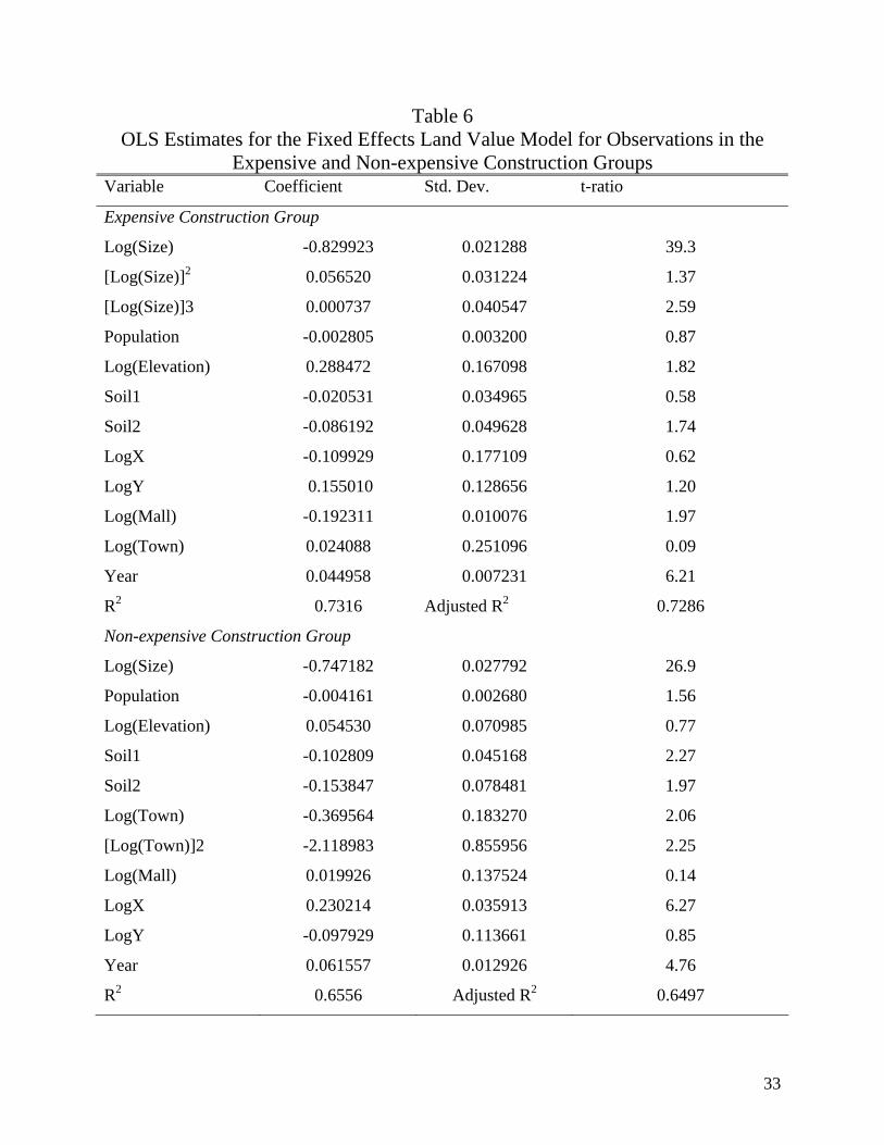
The OLS estimates for models [7] and [8] are presented in Table 6. Coefficient estimates
that are significantly different from zero for at least one of the two models are shown. The
estimated models do not contain the variables “Road” and “LogX*LogY”, because their
coefficients are statistically equal to zero in both models as indicated by the F-statistics reported
for the redundancy test in Table 5. The omission of these variables does not alter the conclusions
of the misspecification tests.
The fixed effects land value model for parcels with expensive construction explains about
73% of the variation in land transaction prices (Table 6). Parcel size is an important determinant
of land value in this group. Larger land parcels are associated with higher land values per square
meter. Higher elevation is associated with higher land values, while weaker evidence indicates
that impermeable soils are associated negatively with land values. Higher elevation and soil
permeability are indicators of lower flood risk. Roanoke County has experienced several floods
in the last fifty years (Roanoke County Planning Department). The model results indicate that
lower flood risk areas have higher land values. Land parcels far from the two major malls are
less expensive perhaps due to the shopping facilities, entertainment amenities, and other services
provided. The average price of land parcels sold in 1997 was higher than in 1996.
The OLS fixed effects land value model for the non-expensive construction parcels
explains about 65% of the variance in land transaction prices. The significance of variables
differs between models for expensive and inexpensive construction. In the inexpensive
construction group, larger parcels have lower land value per square meter. Lack of soil
permeability to water (and consequently higher flood risk as indicated by the Soil1 and Soil2
dummies) is expected to lower land prices. The sign of the elevation parameter is positive but
not statistically significant. There is weak evidence that population density may lower land
18
prices in relatively inexpensive areas. The negative sign of population density may reflect the
willingness of the residents in Roanoke County to live in less populated areas and enjoy open
space amenities. The negative relationship of land values with distance from the nearest town
reflects the effects of distance to amenities and lesser residential and commercial development
potential. The quadratic term of the distance to the nearest town indicates that the parcel value
increases at a decreasing rate when a parcel is closer to the town center. The importance of
location is also reflected by the statistical significance of the coordinate X, which locates the
parcel from southeast to northwest in Roanoke County. The price of lots sold in 1997 was higher
than those sold during the previous year.
Undeveloped Parcels
The fixed effects model [9] was estimated for the group of undeveloped parcels.
Log(Price) = A1[Log(Size)] + A2[Log(Size)]2 + A3[Log(Elevation)] + A4(Population) +
A5(Soil1) + A6(Soil2) + A7[Log(Mall)] + A8[Log(Town)] + A9(Road) + A10(Year) +
A11[Log(X)] + A12[Log(Y)] + A13[Log(X)][Log(Y)] + u [9]
Individual and joint misspecification tests provide support for the assumptions of linearity,
homoskedasticity and structural stability. Low P-values were reported for the Jacque-Bera test
suggesting possible violation of the normality assumptions. However, when some observations
(less than 1%) were excluded from the sample, the P-value of the Jacque-Bera tests exceeded
0.1, and provided support for the assumption of normality. However, the Auxiliary Regression,
ARCH and the Joint Mean and Variance tests have low P values indicating that the assumptions
of no first and second order spatial dependence are violated. This subgroup of parcels is
probably less homogeneous than the two subgroups of developed parcels.
Following Spanos (1986) we estimated a fixed effects model for the vacant parcels,

19
which also allows spatial lags of the dependent and independent variables. Parcels were ordered
by neighborhood. Table 5 indicates that by adding spatial lags in model [9] there is an obvious
improvement in the statistical validity of the model. There is still strong support for the
assumptions of linearity, homoskedasticity and structural stability, while P-values of Auxiliary
Regression and Joint Means tests are also high indicating support for the no spatial
autocorrelation assumptions (both first and second order, respectively). However, there is still
limited support for the hypothesis of no second order spatial dependence (ARCH test). The
coefficients of Year and LogX*LogY and their respective spatial lags are not statistically
different from zero, and the joint F-test recommends dropping these variables from the model.
The final model estimated is [10] and model estimates are shown in Table 7.
Log(Price) = A1[Log(Size)] + A2[Log(Size)]2 + A3(Soil1) + A4(Soil2) + A5[Log(Mall)] +
A6[Log(Town)] + A7(Year) + A8[Log(X)] + A9[Log(Y)] + A10(Road) + A11[WLog(Price)] +
A12[WLog(Size)] + A13(WSoil1) + A14(WSoil2) + A15[WLog(Town)] + A16(WYear) +
A17[WLog(X)] + A18[WLog(Y)] + A19(WRoad) + u [10]
Parcel size is again a significant determinant of land prices, while there is some weak
support for a quadratic relation between parcel size and land price. The quadratic form indicates
that the value of the parcel per square meter decreases at a declining rate with increases in parcel
size. Higher land values should be expected for parcels which are closer to the shopping malls,
but far from town centers. Land value is also lower when the parcel is next to a major road. The
importance of the parcel location is also underlined by the statistical significance of X and Y.
The Year variable again has a positive sign but its value is not statistically important. Finally,
spatial lags are used in addition to fixed neighborhood effects to control for spatial
autocorrelation. The coefficients of spatial lags are larger than the coefficients of the respective
20
explanatory variables implying that neighborhood hedonic characteristics may have stronger
effects on a parcel’s value than the characteristics of that parcel. The signs of spatial lags are
consistent with the signs of their respective explanatory values. For example, an increase in the
size of a parcel and increases in the sizes of the parcels in a neighborhood affect in the same
direction the price of the land parcel. The high R2 value of 0.95 suggests that spatial lags capture
additional variation of the dependent variable in this case study. However, the high R2 value
would have no meaning if the model were not well specified.
Discussion and Conclusions
While the possibility of spatial autocorrelation in cross-sectional models is widely accepted,
current spatial econometric approaches may overlook important factors contributing to observed
spatial autocorrelation. Typically current approaches examine the assumptions of normality,
heteroskedasticity, and structural stability to make sure that observed spatial error autocorrelation
is not due to misspecification problems other than omission of relevant spatial variables. If these
assumptions are satisfied, a spatial error autoregressive model is used to correct for spatial
dependence. However, current spatial econometric studies often test only a subset of
assumptions; test assumptions sequentially; base judgments about model adequacy on fitting
power; and arbitrarily specify model spatial structure. This study finds that reliability of model
estimates is enhanced by basing estimates on a comprehensive set of individual and joint
misspecification tests proposed by Spanos.
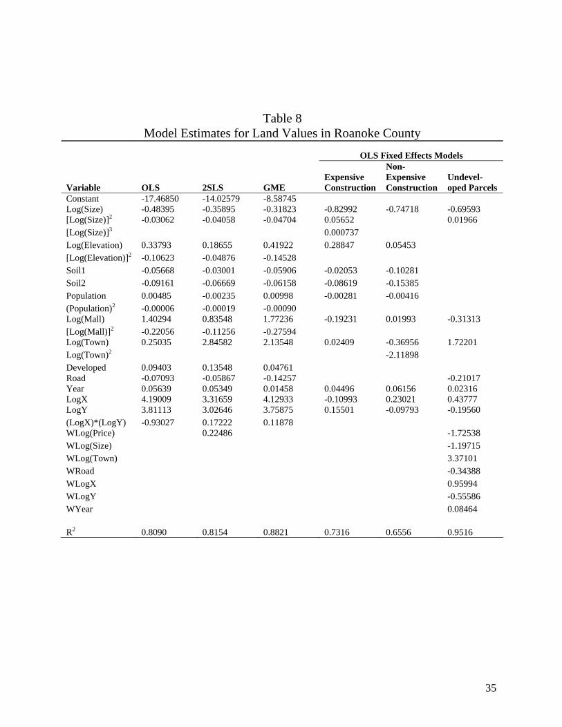
In this study a land value model for Roanoke County was estimated using OLS. Model
results are summarized in Table 8, column 2. The model was tested for spatial autocorrelation
after testing for normality, heteroskedasticity and structural stability. Given the presence of
spatial autocorrelation, parametric and non-parametric estimation techniques were used to
21
account for spatial autocorrelation. Anselin (1988) suggests that the researcher should try
alternative weight matrices to account for neighborhood effects until the misspecification
problem is solved. However, the weight matrix used in this study relies on detailed
neighborhood information provided by the Planning Department of Roanoke County. Results of
the parametric and non-parametric models are shown in Table 8, columns 3 and 4, respectively.
While both techniques achieved higher fitting power (based on R2) than the initial model,
misspecification test results indicate that both models violate essential underlying statistical
assumptions. Given these assumption violations, we conclude that current spatial econometric
techniques do not adequately model land values.
Ultimately three alternative models using OLS and fixed effects of neighborhoods were
estimated to explain the variation in prices of undeveloped parcels, parcels with non-expensive
construction, and parcels with expensive construction in Roanoke County. These models satisfy
the underlying statistical assumptions and, thus, provide more statistically reliable estimates than
the models derived earlier using spatial weight matrices. The study found there was no spatial
dependence in the developed parcel markets but there was spatial dependence in the undeveloped
parcel market. Results are summarized in columns 5, 6, and 7 of Table 8.
Table 8 illustrates several key differences among the models in terms of estimated
impacts of hedonic attributes on land values. First, the OLS, 2SLS, and GME models indicate
that there is a quadratic relationship between parcel size and land value. These three models
agree that land value per square meter decreases with parcel size at a decreasing rate and the
differences in estimated coefficients are small. The alternative OLS fixed effects model was
used to estimate different relationships between parcel size and value which vary by
development status. A negative linear relationship was estimated for developed parcels with
22
non-expensive construction meaning larger parcels have lower values per square meter.
Quadratic relationships were estimated for undeveloped parcels and parcels with expensive
construction. Undeveloped parcel values per square meter declined with size while expensive
parcel values per square meter increased with size.
Second, the effects of elevation and soil, which are proxies for lower flood risk, vary by
model. The OLS, 2SLS, and GME models indicate that higher elevation increases the value of
the parcel at a decreasing rate. All three models indicate that impermeable soil qualities (Soil1
and Soil2) are related to lower land values. Elevation has mixed effects for the OLS fixed effects
models increasing land values for expensive and inexpensive construction, but having no effects
on undeveloped parcel values. Impermeable soils reduce land values for expensive and
inexpensive construction but have no effect on undeveloped parcel values.
Third, with respect to population density, the initial OLS and GME models suggest that
land values increase with higher population density but at a decreasing rate. The 2SLS and the
OLS fixed effects models for developed parcels indicate that increased population density is
related to lower land values. Population density is not significant in the OLS fixed effects model
for undeveloped parcels.
Fourth, the OLS, 2SLS, and GME models suggest that land values increase with
distances from town and mall. The OLS fixed effects models reach a different conclusion.
Longer distance from a mall is related to lower land values for parcels with expensive
construction and undeveloped parcels but higher values for parcels with non-expensive
construction. Longer distance from the nearest town is related to lower land value in the group
of non-expensive parcels but higher values in the expensive construction parcels and
undeveloped parcels.

23
Fifth, the OLS, 2SLS, and GME models indicate negative relationships between parcel
value and location near a major highway. The OLS fixed effects models also indicates a
negative relationship for undeveloped parcels but no relationship for developed parcels.
All models agree that land transaction prices were higher in 1997 than in 1996. At least
one of the location determinants of the parcels (X and Y) is significant in almost all models,
indicating the importance of location even after accounting for neighborhood affects.
The first three models yield relatively higher R2 values than the estimated models for
developed parcels using the OLS fixed effects approach. However, higher fitting power can be
misleading if the model is not well-specified. In addition, the models for developed parcels were
estimated using smaller, more homogeneous samples and, thus, lower variability in the
dependent variable is likely to cause a decline in the fitting power of the models.
Davidson and Mackinnon conclude that in most cases models with apparently correlated
residuals have other specification problems besides error autocorrelation. Future research may
indicate that this is also the case in cross-sectional studies that present spatial autocorrelation.
More work is also needed to corroborate whether developing a statistically adequate model
(Spanos) will make it unnecessary to include arbitrarily specified weight matrices to account for
the influence of surrounding parcels. In cases where spatial lags are needed, more research
would be useful to examine how a simple linear distance performs as a spatial weight matrix
relative to neighborhood boundaries based on socioeconomic and other geographic
characteristics. Finally, further research is needed on the use of a more complete set of
misspecification tests to validate the choice of a weight matrix.
Results of the study have implications for urban expansion to rural areas as well as
government zoning policies. Specifically, the study showed that the type of residential and

24
commercial development (expensive versus non-expensive construction) affects the stochastic
process of land values in Roanoke County. Changes in parcel size have different implications
for land values according to their development status. Smaller parcels may result in higher
values and tax revenue per square meter in areas with non-expensive construction or
undeveloped parcels while smaller parcels may have lower values on a per square meter basis in
areas with expensive construction. More research is necessary to examine how parcel size
affects land value, an issue of importance to local governments concerned with the effects of
development on fiscal revenues and costs and environmental quality.
References
Alston, J. M. and J. A. Chalfant. “Unstable Models and Incorrect Forms.” American Journal of
Agricultural Economics 73(1991): 1171-1181.
Anselin, L. Spatial Econometrics: Methods and Models. Boston: Kluwer Academics, 1988.
Anselin, L. “Spatial Econometrics.” School of Social Sciences, University of Dallas in Texas,
Working Paper, 1999.
Anselin, L., and H. Kelejian. “Testing for Spatial Autocorrelation in the Presence of
Endogenous Regressors.” International Regional Science Review 20(1997): 153-182.
Basu, S., and T. G. Thibodeau. “Analysis of Spatial Correlation in House Prices.” Journal of
Urban Economics 46(1998): 207-218.
Beaton, W.P. “The Impact of Regional Land-Use Controls on Property Values.” Land
Economics 67(1991): 172-194.
Bera, A. K. and C. M. Jarque. “Model Specification Tests: A Simultaneous Approach.”
Journal of Econometrics, Annals 1982-1983: Model Specification 20(1982): 59-82.
Bockstael, N. E., and K. Bell. Land Use Patterns and Water Quality: The Effect of Differential
25
Land Management Controls. Boston: Kluwer Academic Publishers, 1988.
Bosch, D. J., Vinod K. Lohani, Randy L. Dymond, David F. Kibler, and Kurt Stephenson.
“Hydrological and Fiscal Impacts of Residential Development: Virginia Case Study.”
Journal of Water Resources Planning and Management 129(2003): 107-114.
Can, A., and I. Megboludge. “Spatial Dependence and House Price Index Construction.”
Journal of Real Estate Finance and Economics 14(1998): 203-222.
Davidson, R., and MacKinnon J. G. Estimation and Inference in Econometrics. New York:
Oxford University Press, 1993.
Diplas, P., D. Kibler, V.K. Lohani, W. Cox, R. Greene, D.J. Orth, P.S. Nagarkatti, E.F. Benfield,
S. Mostaghimi, R. Gupta, L.A. Shabman, D. J.Bosch, and K. Stephenson. “From
Landscapes to Waterscapes: Integrating Framework for Urbanizing Watersheds.” Project
Proposal for the Environmental Protection Agency and the National Science Foundation,
Blacksburg, Virginia: Virginia Polytechnic Institute and State University, 1997.
Fleming, M, M. “Sample Selection and Spatial Dependence in Hedonic Land Value Models.”
SEA Annual Meeting, University of Maryland at College Park, 1998.
Ghali, M. “Pooling as a Specification Error: A Comment.” Econometrica 45(1977): 755-757.
Irwin, E, G. “Do Spatial Externalities Matter? The Role of Endogenous Interactions in the
Evolution of Land Use Pattern.” University of Maryland, College Park, 1998.
Kaltsas, I. “Spatial Econometrics Revisited: A Case Study of Land Values in Roanoke County.”
Department of Agricultural and Applied Economics. Blacksburg, Virginia, Virginia
Polytechnic Institute and State University, 2000.
Kelejian, H. H., and D. P. Robertson. “A Suggested Method of Estimation for Spatial
Interdependent Models with Autocorrelated Errors, and an Application to a Country
26
Expenditure Model.” Papers in Regional Science 72(1993): 297-312.
Kelejian, H. H., and I. Prucha. “A Generalized Spatial Two Stage Least Squares Procedure for
Estimating a Spatial Autoregressive Model with Autoregressive Disturbances.” Journal
of Real Estate Finance and Economics 17(1998): 99-121.
Kelejian, H. H., and I. Prucha. “A Generalized Moments Estimator for the Autoregressive
Parameter in a Spatial Model.” International Economic Review 31(1999): 68-79.
Lahiri, K. and D. Egy. “Joint Estimation and Testing for Functional Form and
Heteroskedasticity.” Journal of Econometrics 15(1981): 299-307.
Land, K., and G. Deane. “On the Large-Sample Estimation of Regression Models with Spatial
or Network-Effects Terms: A Two Stage Least Square Approach.” Sociological
Methodology 12(1992): 221-48.
McGuirk, A., Driscoll, P., and J. Alwang. “Misspecification Testing: A Comprehensive
Approach.” American Journal of Agricultural Economics 75(1993): 1044-1055.
McGuirk, A., and P. Driscoll. “The Hot Air in R2.” American Journal of Agricultural
Economics 77(1995): 319-328.
Pinkse, J., and I. R. Slade. “Contracting in Space: An Application of Spatial Statistics to
Discrete-Choice Models.” Journal of Econometrics 85(1998): 125-154.
Roanoke County Planning Department. Annual Planning Report, 1994. Roanoke, Virginia,
1994.
Savin, N. E. and K. J. White. “Estimation and Testing for Functional Form and Autocorrelation:
A Simultaneous Approach.” Journal of Econometrics 8(1978): 1-12.
Schmidt, P. Econometrics. New York: Marcel Dekker, 1976.
Spanos, A. Statistical Foundation of Econometric Modeling. Cambridge: Cambridge University

27
Press, 1986.
Xu F., R. C. Mittelhammer, and P. W. Barkley. “Measuring the Contributions of Site
Characteristics to the Value of Agricultural Land.” Land Economics 69(1993): 356-369.

28
Table 1
Descriptive Statistics of Land Values and Explanatory Variables
Variable
Average Std. Dev. Minimum Maximum
Price ($/m2) 23.13 18.08 0.02 133.40
Area (m2) 8,546.53 75,202.91 56.97 2,165,233.00
Elevation (m) 379.82 88.69 3.22 1,003.00
Slope (degrees) 5.49 3.54 0.00 34.56
Soil Qual. 1 0.03 0.17 0.00 1.00
Soil Qual. 2 0.87 0.33 0.00 1.00
Mall 1 (m) 8,861.89 4,281.51 2002.89 27,024.59
Mall 2 (m) 9,246.60 4,774.35 435.92 27,483.35
Roanoke (m) 8,828.68 3,818.12 3,395.87 28,794.36
Blacksburg (m) 39,858.68 6,786.72 18,165.42 51,206.84
Road 0.05 0.22 0.00 1.00
Population (p/Ha) 5.90 4.60 0.05 18.65
Developed 0.88 0.33 0.00 1.00
Coord. Y 16,881.90 6,022.44 1.81 30,585.74
Coord. X 24,888.27 6,766.91 0.15 36,626.16
Year 0.49 0.50 0.00 1.00
29
Table 2
OLS Estimates for the Land Value Model in Roanoke County
Variable Coefficient Std. Dev. t-ratio
Constant -17.46850 3.214461 5.434
Log(Size) -0.483947 0.069485 6.964
[Log(Size)]2 -0.030618 0.009440 3.243
Log(Elevation) 0.337926 0.274165 1.233
[Log(Elevation)]2 -0.106225 0.065750 1.616
Soil1 -0.056682 0.019007 2.982
Soil2 -0.091607 0.036173 2.532
Population 0.004845 0.004217 1.149
(Population)2 -0.000059 0.000023 2.571
Log(Mall) 1.402944 0.417148 3.363
[Log(Mall)]2 -0.220563 0.057922 3.808
Log(Town) 0.250346 0.068201 3.671
Developed 0.094025 0.015405 6.103
Road -0.070932 0.022242 3.189
Year 0.056391 0.009418 5.987
LogX 4.190094 0.732566 5.719
LogY 3.811132 0.695302 5.481
(LogX)*(LogY) -0.930265 0.167058 5.569
R2 0.809
Adjusted R2 0.807
30
Table 3
Misspecification Tests for the OLS Land Value Model Test Null Hypothesis Specification P Value Jacque-Bera
Residuals are normally distributed
JB = (N-k)(4S2+ (K-3)2)/24 S is skewness, K is Kurtosis, and N-k are the degrees of freedom
0.000000
Linearity
Redundancy of non-linear (squared) variables
u = c + ax +bx2 u is the vector of residuals, c is a constant, x is the vector of variables
0.863646
Linearity
Redundancy of non-linear (cross product) variables
u = c + ax +by u is the vector of residuals, u, c, and x as above and y is the vector of cross-product variables
0.154613
White Homoskedasticity u2 = c + ax +bx2 + dy u, c, and x as described above and y is the vector of cross-product variables
0.762358
Auxiliary Regression
No spatial autocorrelation (ordering according to neighborhoods)
U = c + ax +bWu u, c, and x as described above and W is the weight matrix
0.000000
Ramsey RESET
Correctly specified functional form of the model
U = c + ax +bm u, c, and x as described above and m is the vector of fitted values of x
0.932831
ARCH No second order dependence u2z = c + au2
z-1 +bu2z-2 +du3
z-3 u, c, and x as above and z is the ordering factor
0.000000
Chowa Existence of structural change
F statistic based on the comparison of restricted and unrestricted sum of square residuals
>0.2
Fixed Effects No neighborhood fixed effects u = c + aus u, c defined as above, and us is the residual average of a neighborhood
0.000000
First Joint Meanb Linearity, no spatial auto-correlation, structural stability.
u = c + ax + bx2 + dWu + kT u, x, and W as described above and T is a binary variable with 0 before the break point and 1 after
0.000000
Spatial Autocorrelation
No spatial autocorrelation (in the joint mean test)
u = c + ax + bx2 + kT u, x, W, and T as described above
0.000000
Structural Stability Existence of structural change u = c + ax + bx2 +dWu u, x, and W as described above
0.086541
Linearityb Redundancy of non-linear variables
u = c + ax + dWu + kT u, x, W, and T as described above
0.401531
Joint Varianceb Homoskedasticity, no second order dependence and structural stability.
u2z = c + ax + bx2 + du2
z-1 + kT u, c, x, W, z, and T as described above
0.000000
Second Order Dependence
No dependence in residual variance (in joint var. test)
u2z = c + ax + bx2 + kT u, c, x, and T as
described above 0.000000
Structural Stability Structural change (in joint variance test)
u2z = c + ax + bx2 + du2
z-1 u, c, x, and T as described above
0.165318
Homoskedasticity Homoskedasticity (in joint variance test)
u2z = c + ax + bx2 + du2
z-1 + kT u, c, x, and T as described above
0.555664
Second Joint Mean No spatial autocorrelation, no neighborhood fixed effects
u = c + aus + bWu u, c, us, and W defined as above
0.000000
Spatial Autocorrelation
No spatial autocorrelation (in the joint mean test)
U = c + aus u, c, and us as defined above 0.000000
Fixed Effects No neighborhood fixed effects (in the joint mean test)
U = c + bWu u, c, and W defined as above 0.000000
aBreak points at n = 213 and n = 715. bBreak point at n = 213.
31
Table 4
Spatial Two Stage Least Squares Estimates for the Spatial Autoregressive Land
Value Model in Roanoke County
Variable Coefficient Std. Dev. t-ratio
Constant -14.025794 3.342787 4.201
WPRICE 0.224864 0.021740 10.18
Log(Size) -0.358954 0.073127 4.943
[Log(Size)]2 -0.040581 0.009814 4.214
Log(Elevation) 0.186547 0.282630 0.663 [Log(Elevation)]2 -0.048758 0.067642 0.842
Soil1 -0.030005 0.023742 1.672
Soil2 -0.066687 0.037231 1.830
Population -0.002354 0.004381 0.450
(Population)2 -0.000186 0.000241 0.808
Log(Mall) 0.835478 0.436488 1.894
[Log(Mall)]2 -0.112562 0.060764 2.189
Log(Town) 2.845821 0.621488 4.160
Developed 0.135478 0.015608 8.157
Road -0.058667 0.022836 2.653
Year 0.053485 0.009699 5.442
LogX 3.316587 0.755211 4.393 LogY 3.026457 0.716423 4.217
(LogX)*(LogY) -0.655475 0.172219 4.278
pseudo R2 0.815

32
Table 5 Misspecification Tests for Land Value Models for Developed and Undeveloped Parcels
P Values Test Null Hypothesis Specification Expensive
Construction Non-expensive Construction
Undeveloped parcels with spatial lags
Jacque-Bera
Residuals are normally distributed
JB = (N-k)(4S2+ (K-3)2)/24 S is the skewness, K is the Kurtosis, and N-k are the degrees of freedom
0.377409 0.510699 0.000000
Linearity
Redundancy of non-linear (squared) variables
u = c + ax +bx2 u is the vector of residuals, c is a constant, x is the vector of variables
0.548247
0.863646
0.999761
Linearity
Redundancy of non-linear (cross product) variables
u = c + ax +by u is the vector of residuals, c is a constant, y is the vector of cross-product variables
0.128269 0.154613 0.646551
White (Hetero-skedasticity squares)a
Homoskedasticity u2 = c + ax +bx2 + dy u is the vector of residuals, c is a constant, x is the vector of variables, y is the vector of cross-product variables
0.092861 0.112854 0.863646
Auxiliary Regression
No spatial autocorrelation (ordering according to neighborhoods)
u = c + ax +bWu u is the vector of residuals, c is a constant, x is the vector of variables and W is the weighting matrix
0.176971 0.425345 0.425345
Ramsey RESET
Correctly specified functional form of the model
u = c + ax +bz is the vector of residuals, c is a constant, x is the vector of variables and z is the vector of fitted values of x
0.483672 0.932831 0.487500
ARCH No second order dependence u2z = c + au2
z-1 +bu2z-2 +du2
z-3 u is the vector of residuals, c is a constant, x is the vector of variables, z is the ordering factor
0.084552 0.098172 0.001703
Chowb Existence of structural change
F statistic based on the comparison of restricted and unrestricted sum of square residuals
>0.1
>0.1
0.394885
Joint Meanb Linearity, no spatial autocorrelation and structural stability.
u = c + ax2 +bWu + dT u, x, and W as described above and T is a binary variable with 0 before the break point and 1 after
>0.1
>0.1
0.163581
Joint Varianceb Homoskedasticity, no second order dependence and structural stability.
u2z = c + ax2 + bu2
z-1 + dT u, c, x, W, z, and T as described above
>0.1
>0.05
0.076762
Redundancy Variables “Road” and “LogX*LogY” are essential for the land value model.
F-test comparing residual sums of squares for the land value model with and without these variables
0.000000
0.000001 0.000000
aHypothesis test is for b = d = 0. bBreak points of n = 400 and n = 800 for the expensive construction group, n = 200 and n = 400 for the non-expensive construction group, and n = 100 for the undeveloped parcels.
33
Table 6 OLS Estimates for the Fixed Effects Land Value Model for Observations in the
Expensive and Non-expensive Construction Groups Variable Coefficient Std. Dev. t-ratio
Expensive Construction Group
Log(Size) -0.829923 0.021288 39.3
[Log(Size)]2 0.056520 0.031224 1.37
[Log(Size)]3 0.000737 0.040547 2.59
Population -0.002805 0.003200 0.87
Log(Elevation) 0.288472 0.167098 1.82
Soil1 -0.020531 0.034965 0.58
Soil2 -0.086192 0.049628 1.74
LogX -0.109929 0.177109 0.62
LogY 0.155010 0.128656 1.20
Log(Mall) -0.192311 0.010076 1.97
Log(Town) 0.024088 0.251096 0.09
Year 0.044958 0.007231 6.21
R2 0.7316 Adjusted R2 0.7286
Non-expensive Construction Group
Log(Size) -0.747182 0.027792 26.9
Population -0.004161 0.002680 1.56
Log(Elevation) 0.054530 0.070985 0.77
Soil1 -0.102809 0.045168 2.27
Soil2 -0.153847 0.078481 1.97
Log(Town) -0.369564 0.183270 2.06
[Log(Town)]2 -2.118983 0.855956 2.25
Log(Mall) 0.019926 0.137524 0.14
LogX 0.230214 0.035913 6.27
LogY -0.097929 0.113661 0.85
Year 0.061557 0.012926 4.76
R2 0.6556 Adjusted R2 0.6497

34
Table 7
OLS Estimates for the Fixed Effects Land Value Model for Undeveloped Parcels
Variable Coefficient Std. Dev. t-ratio
Log(Size) -0.695926 0.028389 24.5
[Log(Size)]2 0.019661 0.012441 1.58
Log(Mall) -0.313128 0.106184 2.95
Log(Town) 1.722006 0.376349 4.57
Road -0.210169 0.057640 3.64
LogX 0.437769 0.139052 3.15
LogY -0.195595 0.099372 1.97
Year 0.023158 0.020734 1.12
WLog(Price) -1.725382 0.075915 22.7
WLog(Size) -1.197150 0.069400 17.2
WLog(Town) 3.371006 0.844649 3.99
WRoad -0.343883 0.085956 4.00
WLogX 0.959943 0.423241 2.27
WLogY -0.555855 0.272661 2.04
WYear 0.084640 0.047181 1.79
R2 0.9516 Adjusted R2 0.9482
35
Table 8 Model Estimates for Land Values in Roanoke County
OLS Fixed Effects Models
Variable OLS 2SLS GME Expensive Construction
Non-Expensive Construction
Undevel-oped Parcels
Constant -17.46850 -14.02579 -8.58745 Log(Size) -0.48395 -0.35895 -0.31823 -0.82992 -0.74718 -0.69593 [Log(Size)]2 -0.03062 -0.04058 -0.04704 0.05652 0.01966 [Log(Size)]3 0.000737 Log(Elevation) 0.33793 0.18655 0.41922 0.28847 0.05453 [Log(Elevation)]2 -0.10623 -0.04876 -0.14528 Soil1 -0.05668 -0.03001 -0.05906 -0.02053 -0.10281 Soil2 -0.09161 -0.06669 -0.06158 -0.08619 -0.15385 Population 0.00485 -0.00235 0.00998 -0.00281 -0.00416 (Population)2 -0.00006 -0.00019 -0.00090 Log(Mall) 1.40294 0.83548 1.77236 -0.19231 0.01993 -0.31313 [Log(Mall)]2 -0.22056 -0.11256 -0.27594 Log(Town) 0.25035 2.84582 2.13548 0.02409 -0.36956 1.72201 Log(Town)2 -2.11898 Developed 0.09403 0.13548 0.04761 Road -0.07093 -0.05867 -0.14257 -0.21017 Year 0.05639 0.05349 0.01458 0.04496 0.06156 0.02316 LogX 4.19009 3.31659 4.12933 -0.10993 0.23021 0.43777 LogY 3.81113 3.02646 3.75875 0.15501 -0.09793 -0.19560 (LogX)*(LogY) -0.93027 0.17222 0.11878 WLog(Price) 0.22486 -1.72538 WLog(Size) -1.19715 WLog(Town) 3.37101 WRoad -0.34388 WLogX 0.95994 WLogY -0.55586 WYear 0.08464 R2 0.8090 0.8154 0.8821 0.7316 0.6556 0.9516
Top Related