


Languages
Pages
Legal

Sorting
Objectives Become familiar with the following
sorting methods Insertion Sort Shell Sort Selection Sort Bubble Sort Quick Sort Heap Sort Merge Sort hellip more
Introduction One of the most common applications
in computer science is sorting the process through which data are arranged according to their values
If data were not ordered in some way we would spend an incredible amount of time trying to find the correct information
Introduction To appreciate this imagine trying
to find someonersquos number in the telephone book if the names were not sorted in some way
General Sorting Concepts Sorts are generally classified as either
internal or external An internal sort is a sort in which all of
the data is held in primary memory during the sorting process
An external sort uses primary memory for the data currently being sorted and secondary storage for any data that will not fit in primary memory
General Sorting Concepts For example a file of 20000
records may be sorted using an array that holds only 1000 records
Therefore only 1000 records are in primary memory at any given time
The other 19000 records are stored in secondary storage
Sort Order Data may be sorted in either
ascending or descending order The sort order identifies the
sequence of sorted data ascending or descending
If the order of the sort is not specified it is assumed to be ascending
Sort Stability Sort stability is an attribute of a
sort indicating that data elements with equal keys maintain their relative input order in the output
Consider the following example
Sort Stability
Note the unsorted data in (a) If we use a stable sort items with equal keys are
guaranteed to be sorted in the same order as they appear in the unsorted data
Sort Stability
If however we use an unstable sort data with equal keys can be sorted in any order (ie not necessarily in the same order as they appeared in the unsorted data)
Sort Efficiency Sort efficiency is a measure of
the relative efficiency of a sort It is usually an estimate of the
number of comparisons and moves required to order an unordered list
Passes During the sorting process the data is
traversed many times Each traversal of the data is referred to
as a sort pass Depending on the algorithm the sort
pass may traverse the whole list or just a section of the list
The sort pass may also include the placement of one or more elements into the sorted list
Types of Sorts We now discuss several sorting
methods Insertion Sort Shell Sort Selection Sort Bubble Sort Quick Sort Heap Sort Merge Sort
Insertion Sort In each pass of an insertion sort
one or more pieces of data are inserted into their correct location in an ordered list (just as a card player picks up cards and places them in his hand in order)
Insertion Sort In the insertion sort the list is divided into
2 parts Sorted Unsorted
In each pass the first element of the unsorted sublist is transferred to the sorted sublist by inserting it at the appropriate place
If we have a list of n elements it will take at most n-1 passes to sort the data
Insertion Sort
We can visualize this type of sort with the above figure
The first part of the list is the sorted portion which is separated by a ldquoconceptualrdquo wall from the unsorted portion of the list
Insertion SortHere we start with an unsorted list We leave the first data element alone and will start with the 2nd element of the list (the 1st element of the unsorted list)
On our first pass we look at the 2nd element of the list (thefirst element of the unsorted list) and place it in our sorted list in order
On our next pass we look at the 3rd element of the list (the1st element of the unsorted list) and place it in the sorted list in order
We continue in this fashion until the entire list has beensorted
Insertion Sort Example
In our first pass we compare the first 2 values Because theyare out of order we swap them
Now we look at the next 2 values Again they are out oforder so we swap them
Since we have swapped those values we need to comparethe previous 2 values to make sure that they are still in orderSince they are out of order we swap them and then continueon with the next 2 data valuesThese 2 values are out of order so we swap them and look atthe previous 2 values etc
Shell Sort Named after its creator Donald Shell the
shell sort is an improved version of the insertion sort
In the shell sort a list of N elements is divided into K segments where K is known as the increment
What this means is that instead of comparing adjacent values we will compare values that are a distance K apart
We will shrink K as we run through our algorithm
Shell SortPass Notes
1 77 62 14 9 30 21 80 25 70 55 Swap2 21 62 14 9 30 77 80 25 70 55 In order3 21 62 14 9 30 77 80 25 70 55 In order4 21 62 14 9 30 77 80 25 70 55 In order5 21 62 14 9 30 77 80 25 70 55 In order
List (K=5)
Just as in the straight insertion sort we compare 2 values andswap them if they are out of order However in the shell sort we compare values that are a distance K apartOnce we have completed going through the elements in our
list with K=5 we decrease K and continue the process
Shell SortPass Notes
6 21 62 14 9 30 77 80 25 70 55 Swap7 14 62 21 9 30 77 80 25 70 55 Swap8 14 9 21 62 30 77 80 25 70 55 In order9 14 9 21 62 30 77 80 25 70 55 In order10 14 9 21 62 30 77 80 25 70 55 In order11 14 9 21 62 30 77 80 25 70 55 Swap
14 9 21 62 30 25 80 77 70 55 Swap14 9 21 25 30 62 80 77 70 55 In order
12 14 9 21 25 30 62 80 77 70 55 Swap14 9 21 25 30 62 70 77 80 55 In order
13 14 9 21 25 30 62 70 77 80 55 Swap14 9 21 25 30 62 70 55 80 77 Swap14 9 21 25 30 55 70 62 80 77 In order
List (K=2)
Here we have reduced K to 2 Just as in the insertion sort if we swap 2 values we have to go back and compare theprevious 2 values to make sure they are still in order
Shell Sort
All shell sorts will terminate by running an insertion sort(ie K=1) However using the larger values of K first has helped to sort our list so that the straight insertion sort will runfaster
Shell Sort There are many schools of thought
on what the increment should be in the shell sort
Also note that just because an increment is optimal on one list it might not be optimal for another list
Insertion Sort vs Shell Sort Comparing the Big-O notation (for the
average case) we find that Insertion O(n2) Shell O(n125) empirically determined
Although this doesnrsquot seem like much of a gain it makes a big difference as n gets large
Note that in the worst case the Shell sort has an efficiency of O(n2)
However using a special incrementing technique this worst case can be reduced to O(n15)
Insertion Sort vs Shell Sort(Average Case)
Straight Insertion Shell25 625 55100 10000 316500 250000 2364
1000 1000000 56232000 4000000 13374
Number of Loopsn
Selection Sort Imagine some data that you can examine
all at once To sort it you could select the smallest
element and put it in its place select the next smallest and put it in its place etc
For a card player this process is analogous to looking at an entire hand of cards and ordering them by selecting cards one at a time and placing them in their proper order
Selection Sort The selection sort follows this idea Given a list of data to be sorted
we simply select the smallest item and place it in a sorted list
We then repeat these steps until the list is sorted
Selection Sort In the selection sort the list at any moment
is divided into 2 sublists sorted and unsorted separated by a ldquoconceptualrdquo wall
We select the smallest element from the unsorted sublist and exchange it with the element at the beginning of the unsorted data
After each selection and exchange the wall between the 2 sublists moves ndash increasing the number of sorted elements and decreasing the number of unsorted elements
Selection Sort
We start with an unsorted list We search this list for thesmallest element We then exchange the smallest element (8)with the first element in the unsorted list (23)
Again we search the unsorted list for the smallest element We then exchange the smallest element (23) with the first element in the unsorted list (78)
This process continues until the list is fully sorted
Bubble Sort In the bubble sort the list at any
moment is divided into 2 sublists sorted and unsorted
The smallest element is ldquobubbledrdquo from the unsorted sublist to the sorted sublist
Bubble Sort
23 78 45 8 56 3232 56
We start with 32 and compareit with 56 Because 32 is lessthan 56 we swap the twoand step down one element
We then compare 32 and 8Because 32 is not less than 8we do not swap these elements
We step down one element andcompare 45 and 8 They areout of sequence so we swapthem and step down again
8 45
We step down again and compare 8 with 78 These two elements are swapped
8 78
Finally 8 is compared with 23and swapped We thencontinue this process back with56 hellip
8 23
1 Pass of the Bubble Sort
Quick Sort In the bubble sort consecutive items
are compared and possibly exchanged on each pass through the list
This means that many exchanges may be needed to move an element to its correct position
Quick sort is more efficient than bubble sort because a typical exchange involves elements that are far apart so fewer exchanges are required to correctly position an element
Idea of Quick Sort1) Select pick an element
2) Divide rearrange elements so that x goes to its final position E
3) Recurse and Conquer recursively sort
Quick Sort Each iteration of the quick sort
selects an element known as the pivot and divides the list into 3 groups Elements whose keys are less than (or
equal to) the pivotrsquos key The pivot element Elements whose keys are greater than
(or equal to) the pivotrsquos key
Quick Sort The sorting then continues by
quick sorting the left partition followed by quick sorting the right partition
The basic algorithm is as follows
Quick Sort1) Partitioning Step Take an element in the
unsorted array and determine its final location in the sorted array This occurs when all values to the left of the element in the array are less than (or equal to) the element and all values to the right of the element are greater than (or equal to) the element We now have 1 element in its proper location and two unsorted subarrays
2) Recursive Step Perform step 1 on each unsorted subarray
Quick Sort Each time step 1 is performed on a
subarray another element is placed in its final location of the sorted array and two unsorted subarrays are created
When a subarray consists of one element that subarray is sorted
Therefore that element is in its final location
Quick Sort There are several partitioning strategies
used in practice (ie several ldquoversionsrdquo of quick sort) but the one we are about to describe is known to work well
For simplicity we will choose the last element to be the pivot element
We could also chose a different pivot element and swap it with the last element in the array
Quick Sort Below is the array we would like to
sort1 4 8 9 0 11 5 10 7 6
Quick Sort The index left starts at the first element
and right starts at the next-to-last element
We want to move all the elements smaller than the pivot to the left part of the array and all the elements larger than the pivot to the right part
1 4 8 9 0 11 5 10 7 6left righ
t
Quick Sort We move left to the right skipping
over elements that are smaller than the pivot
1 4 8 9 0 11 5 10 7 6left righ
t
Quick Sort We then move right to the left skipping
over elements that are greater than the pivot
When left and right have stopped left is on an element greater than (or equal to) the pivot and right is on an element smaller than (or equal to) the pivot
1 4 8 9 0 11 5 10 7 6left right
Quick Sort If left is to the left of right (or if left
= right) those elements are swapped
1 4 8 9 0 11 5 10 7 6left righ
t
1 4 5 9 0 11 8 10 7 6left righ
t
Quick Sort The effect is to push a large
element to the right and a small element to the left
We then repeat the process until left and right cross
Quick Sort
1 4 5 9 0 11 8 10 7 6left righ
t
1 4 5 9 0 11 8 10 7 6left righ
t
1 4 5 0 9 11 8 10 7 6left righ
t
Quick Sort
1 4 5 0 9 11 8 10 7 6left righ
t
1 4 5 0 9 11 8 10 7 6righ
tleft
Quick Sort
At this point left and right have crossed so no swap is performed
The final part of the partitioning is to swap the pivot element with left
1 4 5 0 9 11 8 10 7 6righ
tleft
1 4 5 0 6 11 8 10 7 9righ
tleft
Quick Sort Note that all elements to the left of
the pivot are less than (or equal to) the pivot and all elements to the right of the pivot are greater than (or equal to) the pivot
Hence the pivot element has been placed in its final sorted position
1 4 5 0 6 11 8 10 7 9righ
tleft
Quick Sort We now repeat the process using
the sub-arrays to the left and right of the pivot
1 4 5 0 6 11 8 10 7 9
1 4 5 0 11 8 10 7 9
Analysis of quicksortmdashbest case
Suppose each partition operation divides the array almost exactly in half
Then the depth of the recursion in log2n Because thatrsquos how many times we can
halve n However there are many recursions at
each level How can we figure this out We note that
Each partition is linear over its subarray All the partitions at one level cover the array
Partitioning at various levels
Best case II We cut the array size in half each time So the depth of the recursion in log2n At each level of the recursion all the
partitions at that level do work that is linear in n
O(log2n) O(n) = O(n log2n)
What about the worst case
Worst case In the worst case partitioning always
divides the size n array into these three parts A length one part containing the pivot itself A length zero part and A length n-1 part containing everything else
We donrsquot recur on the zero-length part Recurring on the length n-1 part requires
(in the worst case) recurring to depth n-1
Worst case partitioning
Worst case for quicksort In the worst case recursion may be
O(n) levels deep (for an array of size n)
But the partitioning work done at each level is still O(n)
O(n) O(n) = O(n2) So worst case for Quicksort is O(n2) When does this happen
When the array is sorted to begin with
Typical case for quicksort If the array is sorted to begin with
Quicksort is terrible O(n2) It is possible to construct other bad
cases However Quicksort is usually O(n log2n) The constants are so good that Quicksort
is generally the fastest algorithm known Most real-world sorting is done by
Quicksort
Tweaking Quicksort Almost anything you can try to
ldquoimproverdquo Quicksort will actually slow it down
One good tweak is to switch to a different sorting method when the subarrays get small (say 10 or 12) Quicksort has too much overhead for small
array sizes For large arrays it might be a good
idea to check beforehand if the array is already sorted But there is a better tweak than this
Randomized Quick-Sort Select the pivot as a random element of the sequence The expected running time of randomized quick-sort on a
sequence of size n is O(n log n) The time spent at a level of the quick-sort tree is O(n) We show that the expected height of the quick-sort tree is
O(log n) good vs bad pivots
bull The probability of a good pivot is 12 thus we expect k2 good pivots out of k pivotsbull After a good pivot the size of each child sequence is at most 34 the size of the parent sequencebull After h pivots we expect (34)h2 n elementsbull The expected height h of the quick-sort tree is at most 2 log43n
Median of three Obviously it doesnrsquot make sense to sort the
array in order to find the median to use as a pivot
Instead compare just three elements of our (sub)arraymdashthe first the last and the middle Take the median (middle value) of these three as
pivot Itrsquos possible (but not easy) to construct cases
which will make this technique O(n2) Suppose we rearrange (sort) these three
numbers so that the smallest is in the first position the largest in the last position and the other in the middle This lets us simplify and speed up the partition
loop
Final comments Weissrsquos code shows some additional
optimizations on pp 246-247 Weiss chooses to stop both searches on
equality to pivot This design decision is debatable
Quicksort is the fastest known general sorting algorithm on average
For optimum speed the pivot must be chosen carefully
ldquoMedian of threerdquo is a good technique for choosing the pivot
There will be some cases where Quicksort runs in O(n2) time
Quick Sort A couple of notes about quick sort There are more optimal ways to
choose the pivot value (such as the median-of-three method)
Also when the subarrays get small it becomes more efficient to use the insertion sort as opposed to continued use of quick sort
Bubble Sort vs Quick Sort If we calculate the Big-O notation
we find that (in the average case) Bubble Sort O(n2) Quick Sort O(nlog2n)
(quick-sort runs in time O(n2) in the worst case)
Heap Sort Idea take the items that need to be
sorted and insert them into the heap By calling deleteHeap we remove the
smallest or largest element depending on whether or not we are working with a min- or max-heap respectively
Hence the elements are removed in ascending or descending order
Efficiency O(nlog2n)
Merge Sort Idea
Take the array you would like to sort and divide it in half to create 2 unsorted subarrays
Next sort each of the 2 subarrays Finally merge the 2 sorted subarrays
into 1 sorted array Efficiency O(nlog2n)
Merge Sort
Merge Sort Although the merge step produces
a sorted array we have overlooked a very important step
How did we sort the 2 halves before performing the merge step
We used merge sort
Merge Sort By continually calling the merge
sort algorithm we eventually get a subarray of size 1
Since an array with only 1 element is clearly sorted we can back out and merge 2 arrays of size 1
Merge Sort
Merge Sort The basic merging algorithm
consists of 2 input arrays (arrayA and arrayB) An ouput array (arrayC) 3 position holders (indexA indexB
indexC) which are initially set to the beginning of their respective arrays
Merge Sort The smaller of arrayA[indexA] and
arrayB[indexB] is copied into arrayC[indexC] and the appropriate position holders are advanced
When either input list is exhausted the remainder of the other list is copied into arrayC
Merge Sort
1 13 24 26index
A
indexC
arrayA
2 15 27 38index
B
arrayB
arrayC
We compare arrayA[indexA]with arrayB[indexB] Whichever value is smaller isplaced into arrayC[indexC]
1 lt 2 so we insert arrayA[indexA] intoarrayC[indexC]
Merge Sort
1 13 24 26indexA
1index
C
arrayA
2 15 27 38index
B
arrayB
arrayC
2 lt 13 so we insert arrayB[indexB] intoarrayC[indexC]
Merge Sort
1 13 24 26indexA
1 2index
C
arrayA
2 15 27 38indexB
arrayB
arrayC
13 lt 15 so we insert arrayA[indexA] intoarrayC[indexC]
Merge Sort
1 13 24 26indexA
1 2 13index
C
arrayA
2 15 27 38indexB
arrayB
arrayC
15 lt 24 so we insert arrayB[indexB] intoarrayC[indexC]
Merge Sort
1 13 24 26indexA
1 2 13 15indexC
arrayA
2 15 27 38indexB
arrayB
arrayC
24 lt 27 so we insert arrayA[indexA] intoarrayC[indexC]
Merge Sort
1 13 24
26
indexA
1 2 13 15 24indexC
arrayA
2 15 27 38indexB
arrayB
arrayC
26 lt 27 so we insert arrayA[indexA] intoarrayC[indexC]
Merge Sort
1 13 24
26
1 2 13 15 24 26indexC
arrayA
2 15 27 38indexB
arrayB
arrayC
Since we have exhaustedone of the arrays arrayAwe simply copy the remaining items from theother array arrayB intoarrayC
Merge Sort
1 13 24
26
1 2 13 15 24 26 27 38
arrayA
2 15 27 38arrayB
arrayC
Efficiency Summary
Sort Worst Case Average Case
Insertion O(n2) O(n2)
Shell O(n15) O(n125)
Selection O(n2) O(n2)
Bubble O(n2) O(n2)
Quick O(n2) O(nlog2n)
Heap O(nlog2n) O(nlog2n)
Merge O(nlog2n) O(nlog2n)
More Sorting
radix sort bucket sort in-place sorting how fast can we sort
Radix Sort
Unlike other sorting methods radix sort considers the structure of the keys
Assume keys are represented in a base M number system (M = radix) ie if M = 2 the keys are represented in binary
Sorting is done by comparing bits in the same position
Extension to keys that are alphanumeric strings
Radix Exchange Sort
Examine bits from left to right1 Sort array with respect to leftmost bit
2 Partition array
3Recursionrecursively sort top subarray ignoring leftmost bitrecursively sort bottom subarray ignoring leftmost bit
Time to sort n b-bit numbers O(b n)
Radix Exchange SortHow do we do the sort from the previous page Same idea as partition in Quicksort repeat
scan top-down to find key starting with 1scan bottom-up to find key starting with 0exchange keys
until scan indices cross
Radix Exchange Sort
Radix Exchange Sort vs Quicksort
Similaritiesboth partition arrayboth recursively sort sub-arrays
DifferencesMethod of partitioning
radix exchange divides array based on greater than or less than 2b-1
quicksort partitions based on greater than or less than some element of the array
Time complexityRadix exchange O (bn)Quicksort average case O (n log n)
Straight Radix Sort
Examines bits from right to left
for k = 0 to b-1 sort the array in a stable waylooking only at bit k
Note order of these bits after sort
Recall ldquosort in a stable
wayrdquo
In a stable sort the initial relative order of equal keys is unchangedFor example observe the first step of the sort from the previous page
Note that the relative order of those keys ending with 0 is unchanged and the same is true for elements ending in 1
The Algorithm is Correct (right)
We show that any two keys are in the correct relative order at the end of the algorithm
Given two keys let k be the leftmost bit-position where they differ
At step k the two keys are put in the correct relative orderBecause of stability the successive steps do not change the relative order of the two keys
For InstanceConsider a sort on an array with these two keys
Radix sorting can be applied to decimal numbers
Straight Radix SortTime Complexity
for k = 0 to b - 1 sort the array in a stable way looking only at bit k
Suppose we can perform the stable sort above in O(n) time The total time complexity would be
O(bn)As you might have guessed we can perform a stable sort based on the keysrsquo kth digit in O(n) time
The method you ask Why itrsquos Bucket Sort of course
Bucket Sort
BASICSn numbersEach number 1 2 3 mStableTime O (n + m)
For example m = 3 and our array is
(note that there are two ldquo2rdquos and two ldquo1rdquos)
First we create M ldquobucketsrdquo
Bucket SortEach element of the array is put in one of the m ldquobucketsrdquo
Bucket Sort
Now pull the elements from the buckets into the array
At last the sorted array (sorted in a stable way)
Comparison Sorting Elements are rearranged by comparing
values of keys Comparison of keys is interleaved with
rearrangements of the order of various pairs of keys as the algorithm progressively moves keys into final sorted order
Comparisons performed at given stage will depend on outcomes of previous comparisons and previous rearrangements of keys
Sorting an array of 3 elements a b and c produces 6 or 3 distinct orderings
Decision TreeConsider a decision tree that sorts n items The next slide shows a decision tree for 3 items a b c
Ovals represent comparisons If lt we traverse down a left branch
otherwise a right branch
Decision Tree on 3 Elements
a b c
bltc
bltc
altb
altc altc
a c b b a cc a b
c b a
b c a
true
true
true true
true
false
false
false
false
false
Levels in Decision Trees Number the levels starting at zero Level i can represent 2i arrangements Our decision tree can represent 8 = 23
arrangements If we have 4 items then 4 = 24 elements
but 4 levels gives at most 24 = 16 so we need 5 levels since 25 = 32 24
If we have k arrangements to represent then we need a decision tree with at least lg k levels
Size of Decision TreeWhen dealing with n elements we have n
possible arrangements and need a decision tree with at least lg n levels
)lg(2
lg2
2lg
2
)2lg()1lg(lg
)1lg()2lg()2lg()1lg(lg
))1)(2)(2)(1(lg()lg(
nn
nn
n
nn
nnn
nnn
nnnn
Lower Bound Resultn = n(n-1)(n-2)hellip21
from this we getlg(n) = lg(n) + lg(n-1) + lg(n-2) +hellip+
lg2 + lg1this means
lg(n) lt nlg(n)and the two results together show
O(lg(n)) = O(nlg(n))
No general sorting algorithm can run faster than O(n lg n)
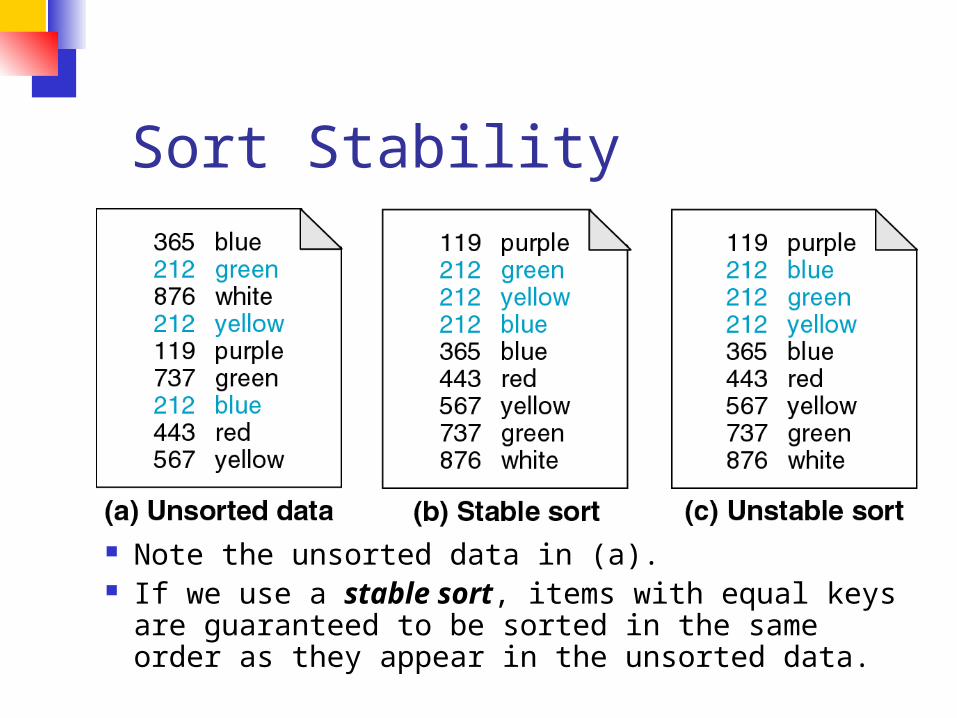
Sort Stability
Note the unsorted data in (a) If we use a stable sort items with equal keys are
guaranteed to be sorted in the same order as they appear in the unsorted data
Sort Stability
If however we use an unstable sort data with equal keys can be sorted in any order (ie not necessarily in the same order as they appeared in the unsorted data)
Sort Efficiency Sort efficiency is a measure of
the relative efficiency of a sort It is usually an estimate of the
number of comparisons and moves required to order an unordered list
Passes During the sorting process the data is
traversed many times Each traversal of the data is referred to
as a sort pass Depending on the algorithm the sort
pass may traverse the whole list or just a section of the list
The sort pass may also include the placement of one or more elements into the sorted list
Types of Sorts We now discuss several sorting
methods Insertion Sort Shell Sort Selection Sort Bubble Sort Quick Sort Heap Sort Merge Sort
Insertion Sort In each pass of an insertion sort
one or more pieces of data are inserted into their correct location in an ordered list (just as a card player picks up cards and places them in his hand in order)
Insertion Sort In the insertion sort the list is divided into
2 parts Sorted Unsorted
In each pass the first element of the unsorted sublist is transferred to the sorted sublist by inserting it at the appropriate place
If we have a list of n elements it will take at most n-1 passes to sort the data
Insertion Sort
We can visualize this type of sort with the above figure
The first part of the list is the sorted portion which is separated by a ldquoconceptualrdquo wall from the unsorted portion of the list
Insertion SortHere we start with an unsorted list We leave the first data element alone and will start with the 2nd element of the list (the 1st element of the unsorted list)
On our first pass we look at the 2nd element of the list (thefirst element of the unsorted list) and place it in our sorted list in order
On our next pass we look at the 3rd element of the list (the1st element of the unsorted list) and place it in the sorted list in order
We continue in this fashion until the entire list has beensorted
Insertion Sort Example
In our first pass we compare the first 2 values Because theyare out of order we swap them
Now we look at the next 2 values Again they are out oforder so we swap them
Since we have swapped those values we need to comparethe previous 2 values to make sure that they are still in orderSince they are out of order we swap them and then continueon with the next 2 data valuesThese 2 values are out of order so we swap them and look atthe previous 2 values etc
Shell Sort Named after its creator Donald Shell the
shell sort is an improved version of the insertion sort
In the shell sort a list of N elements is divided into K segments where K is known as the increment
What this means is that instead of comparing adjacent values we will compare values that are a distance K apart
We will shrink K as we run through our algorithm
Shell SortPass Notes
1 77 62 14 9 30 21 80 25 70 55 Swap2 21 62 14 9 30 77 80 25 70 55 In order3 21 62 14 9 30 77 80 25 70 55 In order4 21 62 14 9 30 77 80 25 70 55 In order5 21 62 14 9 30 77 80 25 70 55 In order
List (K=5)
Just as in the straight insertion sort we compare 2 values andswap them if they are out of order However in the shell sort we compare values that are a distance K apartOnce we have completed going through the elements in our
list with K=5 we decrease K and continue the process
Shell SortPass Notes
6 21 62 14 9 30 77 80 25 70 55 Swap7 14 62 21 9 30 77 80 25 70 55 Swap8 14 9 21 62 30 77 80 25 70 55 In order9 14 9 21 62 30 77 80 25 70 55 In order10 14 9 21 62 30 77 80 25 70 55 In order11 14 9 21 62 30 77 80 25 70 55 Swap
14 9 21 62 30 25 80 77 70 55 Swap14 9 21 25 30 62 80 77 70 55 In order
12 14 9 21 25 30 62 80 77 70 55 Swap14 9 21 25 30 62 70 77 80 55 In order
13 14 9 21 25 30 62 70 77 80 55 Swap14 9 21 25 30 62 70 55 80 77 Swap14 9 21 25 30 55 70 62 80 77 In order
List (K=2)
Here we have reduced K to 2 Just as in the insertion sort if we swap 2 values we have to go back and compare theprevious 2 values to make sure they are still in order
Shell Sort
All shell sorts will terminate by running an insertion sort(ie K=1) However using the larger values of K first has helped to sort our list so that the straight insertion sort will runfaster
Shell Sort There are many schools of thought
on what the increment should be in the shell sort
Also note that just because an increment is optimal on one list it might not be optimal for another list
Insertion Sort vs Shell Sort Comparing the Big-O notation (for the
average case) we find that Insertion O(n2) Shell O(n125) empirically determined
Although this doesnrsquot seem like much of a gain it makes a big difference as n gets large
Note that in the worst case the Shell sort has an efficiency of O(n2)
However using a special incrementing technique this worst case can be reduced to O(n15)
Insertion Sort vs Shell Sort(Average Case)
Straight Insertion Shell25 625 55100 10000 316500 250000 2364
1000 1000000 56232000 4000000 13374
Number of Loopsn
Selection Sort Imagine some data that you can examine
all at once To sort it you could select the smallest
element and put it in its place select the next smallest and put it in its place etc
For a card player this process is analogous to looking at an entire hand of cards and ordering them by selecting cards one at a time and placing them in their proper order
Selection Sort The selection sort follows this idea Given a list of data to be sorted
we simply select the smallest item and place it in a sorted list
We then repeat these steps until the list is sorted
Selection Sort In the selection sort the list at any moment
is divided into 2 sublists sorted and unsorted separated by a ldquoconceptualrdquo wall
We select the smallest element from the unsorted sublist and exchange it with the element at the beginning of the unsorted data
After each selection and exchange the wall between the 2 sublists moves ndash increasing the number of sorted elements and decreasing the number of unsorted elements
Selection Sort
We start with an unsorted list We search this list for thesmallest element We then exchange the smallest element (8)with the first element in the unsorted list (23)
Again we search the unsorted list for the smallest element We then exchange the smallest element (23) with the first element in the unsorted list (78)
This process continues until the list is fully sorted
Bubble Sort In the bubble sort the list at any
moment is divided into 2 sublists sorted and unsorted
The smallest element is ldquobubbledrdquo from the unsorted sublist to the sorted sublist
Bubble Sort
23 78 45 8 56 3232 56
We start with 32 and compareit with 56 Because 32 is lessthan 56 we swap the twoand step down one element
We then compare 32 and 8Because 32 is not less than 8we do not swap these elements
We step down one element andcompare 45 and 8 They areout of sequence so we swapthem and step down again
8 45
We step down again and compare 8 with 78 These two elements are swapped
8 78
Finally 8 is compared with 23and swapped We thencontinue this process back with56 hellip
8 23
1 Pass of the Bubble Sort
Quick Sort In the bubble sort consecutive items
are compared and possibly exchanged on each pass through the list
This means that many exchanges may be needed to move an element to its correct position
Quick sort is more efficient than bubble sort because a typical exchange involves elements that are far apart so fewer exchanges are required to correctly position an element
Idea of Quick Sort1) Select pick an element
2) Divide rearrange elements so that x goes to its final position E
3) Recurse and Conquer recursively sort
Quick Sort Each iteration of the quick sort
selects an element known as the pivot and divides the list into 3 groups Elements whose keys are less than (or
equal to) the pivotrsquos key The pivot element Elements whose keys are greater than
(or equal to) the pivotrsquos key
Quick Sort The sorting then continues by
quick sorting the left partition followed by quick sorting the right partition
The basic algorithm is as follows
Quick Sort1) Partitioning Step Take an element in the
unsorted array and determine its final location in the sorted array This occurs when all values to the left of the element in the array are less than (or equal to) the element and all values to the right of the element are greater than (or equal to) the element We now have 1 element in its proper location and two unsorted subarrays
2) Recursive Step Perform step 1 on each unsorted subarray
Quick Sort Each time step 1 is performed on a
subarray another element is placed in its final location of the sorted array and two unsorted subarrays are created
When a subarray consists of one element that subarray is sorted
Therefore that element is in its final location
Quick Sort There are several partitioning strategies
used in practice (ie several ldquoversionsrdquo of quick sort) but the one we are about to describe is known to work well
For simplicity we will choose the last element to be the pivot element
We could also chose a different pivot element and swap it with the last element in the array
Quick Sort Below is the array we would like to
sort1 4 8 9 0 11 5 10 7 6
Quick Sort The index left starts at the first element
and right starts at the next-to-last element
We want to move all the elements smaller than the pivot to the left part of the array and all the elements larger than the pivot to the right part
1 4 8 9 0 11 5 10 7 6left righ
t
Quick Sort We move left to the right skipping
over elements that are smaller than the pivot
1 4 8 9 0 11 5 10 7 6left righ
t
Quick Sort We then move right to the left skipping
over elements that are greater than the pivot
When left and right have stopped left is on an element greater than (or equal to) the pivot and right is on an element smaller than (or equal to) the pivot
1 4 8 9 0 11 5 10 7 6left right
Quick Sort If left is to the left of right (or if left
= right) those elements are swapped
1 4 8 9 0 11 5 10 7 6left righ
t
1 4 5 9 0 11 8 10 7 6left righ
t
Quick Sort The effect is to push a large
element to the right and a small element to the left
We then repeat the process until left and right cross
Quick Sort
1 4 5 9 0 11 8 10 7 6left righ
t
1 4 5 9 0 11 8 10 7 6left righ
t
1 4 5 0 9 11 8 10 7 6left righ
t
Quick Sort
1 4 5 0 9 11 8 10 7 6left righ
t
1 4 5 0 9 11 8 10 7 6righ
tleft
Quick Sort
At this point left and right have crossed so no swap is performed
The final part of the partitioning is to swap the pivot element with left
1 4 5 0 9 11 8 10 7 6righ
tleft
1 4 5 0 6 11 8 10 7 9righ
tleft
Quick Sort Note that all elements to the left of
the pivot are less than (or equal to) the pivot and all elements to the right of the pivot are greater than (or equal to) the pivot
Hence the pivot element has been placed in its final sorted position
1 4 5 0 6 11 8 10 7 9righ
tleft
Quick Sort We now repeat the process using
the sub-arrays to the left and right of the pivot
1 4 5 0 6 11 8 10 7 9
1 4 5 0 11 8 10 7 9
Analysis of quicksortmdashbest case
Suppose each partition operation divides the array almost exactly in half
Then the depth of the recursion in log2n Because thatrsquos how many times we can
halve n However there are many recursions at
each level How can we figure this out We note that
Each partition is linear over its subarray All the partitions at one level cover the array
Partitioning at various levels
Best case II We cut the array size in half each time So the depth of the recursion in log2n At each level of the recursion all the
partitions at that level do work that is linear in n
O(log2n) O(n) = O(n log2n)
What about the worst case
Worst case In the worst case partitioning always
divides the size n array into these three parts A length one part containing the pivot itself A length zero part and A length n-1 part containing everything else
We donrsquot recur on the zero-length part Recurring on the length n-1 part requires
(in the worst case) recurring to depth n-1
Worst case partitioning
Worst case for quicksort In the worst case recursion may be
O(n) levels deep (for an array of size n)
But the partitioning work done at each level is still O(n)
O(n) O(n) = O(n2) So worst case for Quicksort is O(n2) When does this happen
When the array is sorted to begin with
Typical case for quicksort If the array is sorted to begin with
Quicksort is terrible O(n2) It is possible to construct other bad
cases However Quicksort is usually O(n log2n) The constants are so good that Quicksort
is generally the fastest algorithm known Most real-world sorting is done by
Quicksort
Tweaking Quicksort Almost anything you can try to
ldquoimproverdquo Quicksort will actually slow it down
One good tweak is to switch to a different sorting method when the subarrays get small (say 10 or 12) Quicksort has too much overhead for small
array sizes For large arrays it might be a good
idea to check beforehand if the array is already sorted But there is a better tweak than this
Randomized Quick-Sort Select the pivot as a random element of the sequence The expected running time of randomized quick-sort on a
sequence of size n is O(n log n) The time spent at a level of the quick-sort tree is O(n) We show that the expected height of the quick-sort tree is
O(log n) good vs bad pivots
bull The probability of a good pivot is 12 thus we expect k2 good pivots out of k pivotsbull After a good pivot the size of each child sequence is at most 34 the size of the parent sequencebull After h pivots we expect (34)h2 n elementsbull The expected height h of the quick-sort tree is at most 2 log43n
Median of three Obviously it doesnrsquot make sense to sort the
array in order to find the median to use as a pivot
Instead compare just three elements of our (sub)arraymdashthe first the last and the middle Take the median (middle value) of these three as
pivot Itrsquos possible (but not easy) to construct cases
which will make this technique O(n2) Suppose we rearrange (sort) these three
numbers so that the smallest is in the first position the largest in the last position and the other in the middle This lets us simplify and speed up the partition
loop
Final comments Weissrsquos code shows some additional
optimizations on pp 246-247 Weiss chooses to stop both searches on
equality to pivot This design decision is debatable
Quicksort is the fastest known general sorting algorithm on average
For optimum speed the pivot must be chosen carefully
ldquoMedian of threerdquo is a good technique for choosing the pivot
There will be some cases where Quicksort runs in O(n2) time
Quick Sort A couple of notes about quick sort There are more optimal ways to
choose the pivot value (such as the median-of-three method)
Also when the subarrays get small it becomes more efficient to use the insertion sort as opposed to continued use of quick sort
Bubble Sort vs Quick Sort If we calculate the Big-O notation
we find that (in the average case) Bubble Sort O(n2) Quick Sort O(nlog2n)
(quick-sort runs in time O(n2) in the worst case)
Heap Sort Idea take the items that need to be
sorted and insert them into the heap By calling deleteHeap we remove the
smallest or largest element depending on whether or not we are working with a min- or max-heap respectively
Hence the elements are removed in ascending or descending order
Efficiency O(nlog2n)
Merge Sort Idea
Take the array you would like to sort and divide it in half to create 2 unsorted subarrays
Next sort each of the 2 subarrays Finally merge the 2 sorted subarrays
into 1 sorted array Efficiency O(nlog2n)
Merge Sort
Merge Sort Although the merge step produces
a sorted array we have overlooked a very important step
How did we sort the 2 halves before performing the merge step
We used merge sort
Merge Sort By continually calling the merge
sort algorithm we eventually get a subarray of size 1
Since an array with only 1 element is clearly sorted we can back out and merge 2 arrays of size 1
Merge Sort
Merge Sort The basic merging algorithm
consists of 2 input arrays (arrayA and arrayB) An ouput array (arrayC) 3 position holders (indexA indexB
indexC) which are initially set to the beginning of their respective arrays
Merge Sort The smaller of arrayA[indexA] and
arrayB[indexB] is copied into arrayC[indexC] and the appropriate position holders are advanced
When either input list is exhausted the remainder of the other list is copied into arrayC
Merge Sort
1 13 24 26index
A
indexC
arrayA
2 15 27 38index
B
arrayB
arrayC
We compare arrayA[indexA]with arrayB[indexB] Whichever value is smaller isplaced into arrayC[indexC]
1 lt 2 so we insert arrayA[indexA] intoarrayC[indexC]
Merge Sort
1 13 24 26indexA
1index
C
arrayA
2 15 27 38index
B
arrayB
arrayC
2 lt 13 so we insert arrayB[indexB] intoarrayC[indexC]
Merge Sort
1 13 24 26indexA
1 2index
C
arrayA
2 15 27 38indexB
arrayB
arrayC
13 lt 15 so we insert arrayA[indexA] intoarrayC[indexC]
Merge Sort
1 13 24 26indexA
1 2 13index
C
arrayA
2 15 27 38indexB
arrayB
arrayC
15 lt 24 so we insert arrayB[indexB] intoarrayC[indexC]
Merge Sort
1 13 24 26indexA
1 2 13 15indexC
arrayA
2 15 27 38indexB
arrayB
arrayC
24 lt 27 so we insert arrayA[indexA] intoarrayC[indexC]
Merge Sort
1 13 24
26
indexA
1 2 13 15 24indexC
arrayA
2 15 27 38indexB
arrayB
arrayC
26 lt 27 so we insert arrayA[indexA] intoarrayC[indexC]
Merge Sort
1 13 24
26
1 2 13 15 24 26indexC
arrayA
2 15 27 38indexB
arrayB
arrayC
Since we have exhaustedone of the arrays arrayAwe simply copy the remaining items from theother array arrayB intoarrayC
Merge Sort
1 13 24
26
1 2 13 15 24 26 27 38
arrayA
2 15 27 38arrayB
arrayC
Efficiency Summary
Sort Worst Case Average Case
Insertion O(n2) O(n2)
Shell O(n15) O(n125)
Selection O(n2) O(n2)
Bubble O(n2) O(n2)
Quick O(n2) O(nlog2n)
Heap O(nlog2n) O(nlog2n)
Merge O(nlog2n) O(nlog2n)
More Sorting
radix sort bucket sort in-place sorting how fast can we sort
Radix Sort
Unlike other sorting methods radix sort considers the structure of the keys
Assume keys are represented in a base M number system (M = radix) ie if M = 2 the keys are represented in binary
Sorting is done by comparing bits in the same position
Extension to keys that are alphanumeric strings
Radix Exchange Sort
Examine bits from left to right1 Sort array with respect to leftmost bit
2 Partition array
3Recursionrecursively sort top subarray ignoring leftmost bitrecursively sort bottom subarray ignoring leftmost bit
Time to sort n b-bit numbers O(b n)
Radix Exchange SortHow do we do the sort from the previous page Same idea as partition in Quicksort repeat
scan top-down to find key starting with 1scan bottom-up to find key starting with 0exchange keys
until scan indices cross
Radix Exchange Sort
Radix Exchange Sort vs Quicksort
Similaritiesboth partition arrayboth recursively sort sub-arrays
DifferencesMethod of partitioning
radix exchange divides array based on greater than or less than 2b-1
quicksort partitions based on greater than or less than some element of the array
Time complexityRadix exchange O (bn)Quicksort average case O (n log n)
Straight Radix Sort
Examines bits from right to left
for k = 0 to b-1 sort the array in a stable waylooking only at bit k
Note order of these bits after sort
Recall ldquosort in a stable
wayrdquo
In a stable sort the initial relative order of equal keys is unchangedFor example observe the first step of the sort from the previous page
Note that the relative order of those keys ending with 0 is unchanged and the same is true for elements ending in 1
The Algorithm is Correct (right)
We show that any two keys are in the correct relative order at the end of the algorithm
Given two keys let k be the leftmost bit-position where they differ
At step k the two keys are put in the correct relative orderBecause of stability the successive steps do not change the relative order of the two keys
For InstanceConsider a sort on an array with these two keys
Radix sorting can be applied to decimal numbers
Straight Radix SortTime Complexity
for k = 0 to b - 1 sort the array in a stable way looking only at bit k
Suppose we can perform the stable sort above in O(n) time The total time complexity would be
O(bn)As you might have guessed we can perform a stable sort based on the keysrsquo kth digit in O(n) time
The method you ask Why itrsquos Bucket Sort of course
Bucket Sort
BASICSn numbersEach number 1 2 3 mStableTime O (n + m)
For example m = 3 and our array is
(note that there are two ldquo2rdquos and two ldquo1rdquos)
First we create M ldquobucketsrdquo
Bucket SortEach element of the array is put in one of the m ldquobucketsrdquo
Bucket Sort
Now pull the elements from the buckets into the array
At last the sorted array (sorted in a stable way)
Comparison Sorting Elements are rearranged by comparing
values of keys Comparison of keys is interleaved with
rearrangements of the order of various pairs of keys as the algorithm progressively moves keys into final sorted order
Comparisons performed at given stage will depend on outcomes of previous comparisons and previous rearrangements of keys
Sorting an array of 3 elements a b and c produces 6 or 3 distinct orderings
Decision TreeConsider a decision tree that sorts n items The next slide shows a decision tree for 3 items a b c
Ovals represent comparisons If lt we traverse down a left branch
otherwise a right branch
Decision Tree on 3 Elements
a b c
bltc
bltc
altb
altc altc
a c b b a cc a b
c b a
b c a
true
true
true true
true
false
false
false
false
false
Levels in Decision Trees Number the levels starting at zero Level i can represent 2i arrangements Our decision tree can represent 8 = 23
arrangements If we have 4 items then 4 = 24 elements
but 4 levels gives at most 24 = 16 so we need 5 levels since 25 = 32 24
If we have k arrangements to represent then we need a decision tree with at least lg k levels
Size of Decision TreeWhen dealing with n elements we have n
possible arrangements and need a decision tree with at least lg n levels
)lg(2
lg2
2lg
2
)2lg()1lg(lg
)1lg()2lg()2lg()1lg(lg
))1)(2)(2)(1(lg()lg(
nn
nn
n
nn
nnn
nnn
nnnn
Lower Bound Resultn = n(n-1)(n-2)hellip21
from this we getlg(n) = lg(n) + lg(n-1) + lg(n-2) +hellip+
lg2 + lg1this means
lg(n) lt nlg(n)and the two results together show
O(lg(n)) = O(nlg(n))
No general sorting algorithm can run faster than O(n lg n)
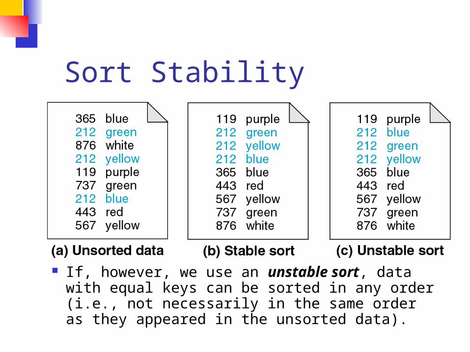
Sort Stability
If however we use an unstable sort data with equal keys can be sorted in any order (ie not necessarily in the same order as they appeared in the unsorted data)
Sort Efficiency Sort efficiency is a measure of
the relative efficiency of a sort It is usually an estimate of the
number of comparisons and moves required to order an unordered list
Passes During the sorting process the data is
traversed many times Each traversal of the data is referred to
as a sort pass Depending on the algorithm the sort
pass may traverse the whole list or just a section of the list
The sort pass may also include the placement of one or more elements into the sorted list
Types of Sorts We now discuss several sorting
methods Insertion Sort Shell Sort Selection Sort Bubble Sort Quick Sort Heap Sort Merge Sort
Insertion Sort In each pass of an insertion sort
one or more pieces of data are inserted into their correct location in an ordered list (just as a card player picks up cards and places them in his hand in order)
Insertion Sort In the insertion sort the list is divided into
2 parts Sorted Unsorted
In each pass the first element of the unsorted sublist is transferred to the sorted sublist by inserting it at the appropriate place
If we have a list of n elements it will take at most n-1 passes to sort the data
Insertion Sort
We can visualize this type of sort with the above figure
The first part of the list is the sorted portion which is separated by a ldquoconceptualrdquo wall from the unsorted portion of the list
Insertion SortHere we start with an unsorted list We leave the first data element alone and will start with the 2nd element of the list (the 1st element of the unsorted list)
On our first pass we look at the 2nd element of the list (thefirst element of the unsorted list) and place it in our sorted list in order
On our next pass we look at the 3rd element of the list (the1st element of the unsorted list) and place it in the sorted list in order
We continue in this fashion until the entire list has beensorted
Insertion Sort Example
In our first pass we compare the first 2 values Because theyare out of order we swap them
Now we look at the next 2 values Again they are out oforder so we swap them
Since we have swapped those values we need to comparethe previous 2 values to make sure that they are still in orderSince they are out of order we swap them and then continueon with the next 2 data valuesThese 2 values are out of order so we swap them and look atthe previous 2 values etc
Shell Sort Named after its creator Donald Shell the
shell sort is an improved version of the insertion sort
In the shell sort a list of N elements is divided into K segments where K is known as the increment
What this means is that instead of comparing adjacent values we will compare values that are a distance K apart
We will shrink K as we run through our algorithm
Shell SortPass Notes
1 77 62 14 9 30 21 80 25 70 55 Swap2 21 62 14 9 30 77 80 25 70 55 In order3 21 62 14 9 30 77 80 25 70 55 In order4 21 62 14 9 30 77 80 25 70 55 In order5 21 62 14 9 30 77 80 25 70 55 In order
List (K=5)
Just as in the straight insertion sort we compare 2 values andswap them if they are out of order However in the shell sort we compare values that are a distance K apartOnce we have completed going through the elements in our
list with K=5 we decrease K and continue the process
Shell SortPass Notes
6 21 62 14 9 30 77 80 25 70 55 Swap7 14 62 21 9 30 77 80 25 70 55 Swap8 14 9 21 62 30 77 80 25 70 55 In order9 14 9 21 62 30 77 80 25 70 55 In order10 14 9 21 62 30 77 80 25 70 55 In order11 14 9 21 62 30 77 80 25 70 55 Swap
14 9 21 62 30 25 80 77 70 55 Swap14 9 21 25 30 62 80 77 70 55 In order
12 14 9 21 25 30 62 80 77 70 55 Swap14 9 21 25 30 62 70 77 80 55 In order
13 14 9 21 25 30 62 70 77 80 55 Swap14 9 21 25 30 62 70 55 80 77 Swap14 9 21 25 30 55 70 62 80 77 In order
List (K=2)
Here we have reduced K to 2 Just as in the insertion sort if we swap 2 values we have to go back and compare theprevious 2 values to make sure they are still in order
Shell Sort
All shell sorts will terminate by running an insertion sort(ie K=1) However using the larger values of K first has helped to sort our list so that the straight insertion sort will runfaster
Shell Sort There are many schools of thought
on what the increment should be in the shell sort
Also note that just because an increment is optimal on one list it might not be optimal for another list
Insertion Sort vs Shell Sort Comparing the Big-O notation (for the
average case) we find that Insertion O(n2) Shell O(n125) empirically determined
Although this doesnrsquot seem like much of a gain it makes a big difference as n gets large
Note that in the worst case the Shell sort has an efficiency of O(n2)
However using a special incrementing technique this worst case can be reduced to O(n15)
Insertion Sort vs Shell Sort(Average Case)
Straight Insertion Shell25 625 55100 10000 316500 250000 2364
1000 1000000 56232000 4000000 13374
Number of Loopsn
Selection Sort Imagine some data that you can examine
all at once To sort it you could select the smallest
element and put it in its place select the next smallest and put it in its place etc
For a card player this process is analogous to looking at an entire hand of cards and ordering them by selecting cards one at a time and placing them in their proper order
Selection Sort The selection sort follows this idea Given a list of data to be sorted
we simply select the smallest item and place it in a sorted list
We then repeat these steps until the list is sorted
Selection Sort In the selection sort the list at any moment
is divided into 2 sublists sorted and unsorted separated by a ldquoconceptualrdquo wall
We select the smallest element from the unsorted sublist and exchange it with the element at the beginning of the unsorted data
After each selection and exchange the wall between the 2 sublists moves ndash increasing the number of sorted elements and decreasing the number of unsorted elements
Selection Sort
We start with an unsorted list We search this list for thesmallest element We then exchange the smallest element (8)with the first element in the unsorted list (23)
Again we search the unsorted list for the smallest element We then exchange the smallest element (23) with the first element in the unsorted list (78)
This process continues until the list is fully sorted
Bubble Sort In the bubble sort the list at any
moment is divided into 2 sublists sorted and unsorted
The smallest element is ldquobubbledrdquo from the unsorted sublist to the sorted sublist
Bubble Sort
23 78 45 8 56 3232 56
We start with 32 and compareit with 56 Because 32 is lessthan 56 we swap the twoand step down one element
We then compare 32 and 8Because 32 is not less than 8we do not swap these elements
We step down one element andcompare 45 and 8 They areout of sequence so we swapthem and step down again
8 45
We step down again and compare 8 with 78 These two elements are swapped
8 78
Finally 8 is compared with 23and swapped We thencontinue this process back with56 hellip
8 23
1 Pass of the Bubble Sort
Quick Sort In the bubble sort consecutive items
are compared and possibly exchanged on each pass through the list
This means that many exchanges may be needed to move an element to its correct position
Quick sort is more efficient than bubble sort because a typical exchange involves elements that are far apart so fewer exchanges are required to correctly position an element
Idea of Quick Sort1) Select pick an element
2) Divide rearrange elements so that x goes to its final position E
3) Recurse and Conquer recursively sort
Quick Sort Each iteration of the quick sort
selects an element known as the pivot and divides the list into 3 groups Elements whose keys are less than (or
equal to) the pivotrsquos key The pivot element Elements whose keys are greater than
(or equal to) the pivotrsquos key
Quick Sort The sorting then continues by
quick sorting the left partition followed by quick sorting the right partition
The basic algorithm is as follows
Quick Sort1) Partitioning Step Take an element in the
unsorted array and determine its final location in the sorted array This occurs when all values to the left of the element in the array are less than (or equal to) the element and all values to the right of the element are greater than (or equal to) the element We now have 1 element in its proper location and two unsorted subarrays
2) Recursive Step Perform step 1 on each unsorted subarray
Quick Sort Each time step 1 is performed on a
subarray another element is placed in its final location of the sorted array and two unsorted subarrays are created
When a subarray consists of one element that subarray is sorted
Therefore that element is in its final location
Quick Sort There are several partitioning strategies
used in practice (ie several ldquoversionsrdquo of quick sort) but the one we are about to describe is known to work well
For simplicity we will choose the last element to be the pivot element
We could also chose a different pivot element and swap it with the last element in the array
Quick Sort Below is the array we would like to
sort1 4 8 9 0 11 5 10 7 6
Quick Sort The index left starts at the first element
and right starts at the next-to-last element
We want to move all the elements smaller than the pivot to the left part of the array and all the elements larger than the pivot to the right part
1 4 8 9 0 11 5 10 7 6left righ
t
Quick Sort We move left to the right skipping
over elements that are smaller than the pivot
1 4 8 9 0 11 5 10 7 6left righ
t
Quick Sort We then move right to the left skipping
over elements that are greater than the pivot
When left and right have stopped left is on an element greater than (or equal to) the pivot and right is on an element smaller than (or equal to) the pivot
1 4 8 9 0 11 5 10 7 6left right
Quick Sort If left is to the left of right (or if left
= right) those elements are swapped
1 4 8 9 0 11 5 10 7 6left righ
t
1 4 5 9 0 11 8 10 7 6left righ
t
Quick Sort The effect is to push a large
element to the right and a small element to the left
We then repeat the process until left and right cross
Quick Sort
1 4 5 9 0 11 8 10 7 6left righ
t
1 4 5 9 0 11 8 10 7 6left righ
t
1 4 5 0 9 11 8 10 7 6left righ
t
Quick Sort
1 4 5 0 9 11 8 10 7 6left righ
t
1 4 5 0 9 11 8 10 7 6righ
tleft
Quick Sort
At this point left and right have crossed so no swap is performed
The final part of the partitioning is to swap the pivot element with left
1 4 5 0 9 11 8 10 7 6righ
tleft
1 4 5 0 6 11 8 10 7 9righ
tleft
Quick Sort Note that all elements to the left of
the pivot are less than (or equal to) the pivot and all elements to the right of the pivot are greater than (or equal to) the pivot
Hence the pivot element has been placed in its final sorted position
1 4 5 0 6 11 8 10 7 9righ
tleft
Quick Sort We now repeat the process using
the sub-arrays to the left and right of the pivot
1 4 5 0 6 11 8 10 7 9
1 4 5 0 11 8 10 7 9
Analysis of quicksortmdashbest case
Suppose each partition operation divides the array almost exactly in half
Then the depth of the recursion in log2n Because thatrsquos how many times we can
halve n However there are many recursions at
each level How can we figure this out We note that
Each partition is linear over its subarray All the partitions at one level cover the array
Partitioning at various levels
Best case II We cut the array size in half each time So the depth of the recursion in log2n At each level of the recursion all the
partitions at that level do work that is linear in n
O(log2n) O(n) = O(n log2n)
What about the worst case
Worst case In the worst case partitioning always
divides the size n array into these three parts A length one part containing the pivot itself A length zero part and A length n-1 part containing everything else
We donrsquot recur on the zero-length part Recurring on the length n-1 part requires
(in the worst case) recurring to depth n-1
Worst case partitioning
Worst case for quicksort In the worst case recursion may be
O(n) levels deep (for an array of size n)
But the partitioning work done at each level is still O(n)
O(n) O(n) = O(n2) So worst case for Quicksort is O(n2) When does this happen
When the array is sorted to begin with
Typical case for quicksort If the array is sorted to begin with
Quicksort is terrible O(n2) It is possible to construct other bad
cases However Quicksort is usually O(n log2n) The constants are so good that Quicksort
is generally the fastest algorithm known Most real-world sorting is done by
Quicksort
Tweaking Quicksort Almost anything you can try to
ldquoimproverdquo Quicksort will actually slow it down
One good tweak is to switch to a different sorting method when the subarrays get small (say 10 or 12) Quicksort has too much overhead for small
array sizes For large arrays it might be a good
idea to check beforehand if the array is already sorted But there is a better tweak than this
Randomized Quick-Sort Select the pivot as a random element of the sequence The expected running time of randomized quick-sort on a
sequence of size n is O(n log n) The time spent at a level of the quick-sort tree is O(n) We show that the expected height of the quick-sort tree is
O(log n) good vs bad pivots
bull The probability of a good pivot is 12 thus we expect k2 good pivots out of k pivotsbull After a good pivot the size of each child sequence is at most 34 the size of the parent sequencebull After h pivots we expect (34)h2 n elementsbull The expected height h of the quick-sort tree is at most 2 log43n
Median of three Obviously it doesnrsquot make sense to sort the
array in order to find the median to use as a pivot
Instead compare just three elements of our (sub)arraymdashthe first the last and the middle Take the median (middle value) of these three as
pivot Itrsquos possible (but not easy) to construct cases
which will make this technique O(n2) Suppose we rearrange (sort) these three
numbers so that the smallest is in the first position the largest in the last position and the other in the middle This lets us simplify and speed up the partition
loop
Final comments Weissrsquos code shows some additional
optimizations on pp 246-247 Weiss chooses to stop both searches on
equality to pivot This design decision is debatable
Quicksort is the fastest known general sorting algorithm on average
For optimum speed the pivot must be chosen carefully
ldquoMedian of threerdquo is a good technique for choosing the pivot
There will be some cases where Quicksort runs in O(n2) time
Quick Sort A couple of notes about quick sort There are more optimal ways to
choose the pivot value (such as the median-of-three method)
Also when the subarrays get small it becomes more efficient to use the insertion sort as opposed to continued use of quick sort
Bubble Sort vs Quick Sort If we calculate the Big-O notation
we find that (in the average case) Bubble Sort O(n2) Quick Sort O(nlog2n)
(quick-sort runs in time O(n2) in the worst case)
Heap Sort Idea take the items that need to be
sorted and insert them into the heap By calling deleteHeap we remove the
smallest or largest element depending on whether or not we are working with a min- or max-heap respectively
Hence the elements are removed in ascending or descending order
Efficiency O(nlog2n)
Merge Sort Idea
Take the array you would like to sort and divide it in half to create 2 unsorted subarrays
Next sort each of the 2 subarrays Finally merge the 2 sorted subarrays
into 1 sorted array Efficiency O(nlog2n)
Merge Sort
Merge Sort Although the merge step produces
a sorted array we have overlooked a very important step
How did we sort the 2 halves before performing the merge step
We used merge sort
Merge Sort By continually calling the merge
sort algorithm we eventually get a subarray of size 1
Since an array with only 1 element is clearly sorted we can back out and merge 2 arrays of size 1
Merge Sort
Merge Sort The basic merging algorithm
consists of 2 input arrays (arrayA and arrayB) An ouput array (arrayC) 3 position holders (indexA indexB
indexC) which are initially set to the beginning of their respective arrays
Merge Sort The smaller of arrayA[indexA] and
arrayB[indexB] is copied into arrayC[indexC] and the appropriate position holders are advanced
When either input list is exhausted the remainder of the other list is copied into arrayC
Merge Sort
1 13 24 26index
A
indexC
arrayA
2 15 27 38index
B
arrayB
arrayC
We compare arrayA[indexA]with arrayB[indexB] Whichever value is smaller isplaced into arrayC[indexC]
1 lt 2 so we insert arrayA[indexA] intoarrayC[indexC]
Merge Sort
1 13 24 26indexA
1index
C
arrayA
2 15 27 38index
B
arrayB
arrayC
2 lt 13 so we insert arrayB[indexB] intoarrayC[indexC]
Merge Sort
1 13 24 26indexA
1 2index
C
arrayA
2 15 27 38indexB
arrayB
arrayC
13 lt 15 so we insert arrayA[indexA] intoarrayC[indexC]
Merge Sort
1 13 24 26indexA
1 2 13index
C
arrayA
2 15 27 38indexB
arrayB
arrayC
15 lt 24 so we insert arrayB[indexB] intoarrayC[indexC]
Merge Sort
1 13 24 26indexA
1 2 13 15indexC
arrayA
2 15 27 38indexB
arrayB
arrayC
24 lt 27 so we insert arrayA[indexA] intoarrayC[indexC]
Merge Sort
1 13 24
26
indexA
1 2 13 15 24indexC
arrayA
2 15 27 38indexB
arrayB
arrayC
26 lt 27 so we insert arrayA[indexA] intoarrayC[indexC]
Merge Sort
1 13 24
26
1 2 13 15 24 26indexC
arrayA
2 15 27 38indexB
arrayB
arrayC
Since we have exhaustedone of the arrays arrayAwe simply copy the remaining items from theother array arrayB intoarrayC
Merge Sort
1 13 24
26
1 2 13 15 24 26 27 38
arrayA
2 15 27 38arrayB
arrayC
Efficiency Summary
Sort Worst Case Average Case
Insertion O(n2) O(n2)
Shell O(n15) O(n125)
Selection O(n2) O(n2)
Bubble O(n2) O(n2)
Quick O(n2) O(nlog2n)
Heap O(nlog2n) O(nlog2n)
Merge O(nlog2n) O(nlog2n)
More Sorting
radix sort bucket sort in-place sorting how fast can we sort
Radix Sort
Unlike other sorting methods radix sort considers the structure of the keys
Assume keys are represented in a base M number system (M = radix) ie if M = 2 the keys are represented in binary
Sorting is done by comparing bits in the same position
Extension to keys that are alphanumeric strings
Radix Exchange Sort
Examine bits from left to right1 Sort array with respect to leftmost bit
2 Partition array
3Recursionrecursively sort top subarray ignoring leftmost bitrecursively sort bottom subarray ignoring leftmost bit
Time to sort n b-bit numbers O(b n)
Radix Exchange SortHow do we do the sort from the previous page Same idea as partition in Quicksort repeat
scan top-down to find key starting with 1scan bottom-up to find key starting with 0exchange keys
until scan indices cross
Radix Exchange Sort
Radix Exchange Sort vs Quicksort
Similaritiesboth partition arrayboth recursively sort sub-arrays
DifferencesMethod of partitioning
radix exchange divides array based on greater than or less than 2b-1
quicksort partitions based on greater than or less than some element of the array
Time complexityRadix exchange O (bn)Quicksort average case O (n log n)
Straight Radix Sort
Examines bits from right to left
for k = 0 to b-1 sort the array in a stable waylooking only at bit k
Note order of these bits after sort
Recall ldquosort in a stable
wayrdquo
In a stable sort the initial relative order of equal keys is unchangedFor example observe the first step of the sort from the previous page
Note that the relative order of those keys ending with 0 is unchanged and the same is true for elements ending in 1
The Algorithm is Correct (right)
We show that any two keys are in the correct relative order at the end of the algorithm
Given two keys let k be the leftmost bit-position where they differ
At step k the two keys are put in the correct relative orderBecause of stability the successive steps do not change the relative order of the two keys
For InstanceConsider a sort on an array with these two keys
Radix sorting can be applied to decimal numbers
Straight Radix SortTime Complexity
for k = 0 to b - 1 sort the array in a stable way looking only at bit k
Suppose we can perform the stable sort above in O(n) time The total time complexity would be
O(bn)As you might have guessed we can perform a stable sort based on the keysrsquo kth digit in O(n) time
The method you ask Why itrsquos Bucket Sort of course
Bucket Sort
BASICSn numbersEach number 1 2 3 mStableTime O (n + m)
For example m = 3 and our array is
(note that there are two ldquo2rdquos and two ldquo1rdquos)
First we create M ldquobucketsrdquo
Bucket SortEach element of the array is put in one of the m ldquobucketsrdquo
Bucket Sort
Now pull the elements from the buckets into the array
At last the sorted array (sorted in a stable way)
Comparison Sorting Elements are rearranged by comparing
values of keys Comparison of keys is interleaved with
rearrangements of the order of various pairs of keys as the algorithm progressively moves keys into final sorted order
Comparisons performed at given stage will depend on outcomes of previous comparisons and previous rearrangements of keys
Sorting an array of 3 elements a b and c produces 6 or 3 distinct orderings
Decision TreeConsider a decision tree that sorts n items The next slide shows a decision tree for 3 items a b c
Ovals represent comparisons If lt we traverse down a left branch
otherwise a right branch
Decision Tree on 3 Elements
a b c
bltc
bltc
altb
altc altc
a c b b a cc a b
c b a
b c a
true
true
true true
true
false
false
false
false
false
Levels in Decision Trees Number the levels starting at zero Level i can represent 2i arrangements Our decision tree can represent 8 = 23
arrangements If we have 4 items then 4 = 24 elements
but 4 levels gives at most 24 = 16 so we need 5 levels since 25 = 32 24
If we have k arrangements to represent then we need a decision tree with at least lg k levels
Size of Decision TreeWhen dealing with n elements we have n
possible arrangements and need a decision tree with at least lg n levels
)lg(2
lg2
2lg
2
)2lg()1lg(lg
)1lg()2lg()2lg()1lg(lg
))1)(2)(2)(1(lg()lg(
nn
nn
n
nn
nnn
nnn
nnnn
Lower Bound Resultn = n(n-1)(n-2)hellip21
from this we getlg(n) = lg(n) + lg(n-1) + lg(n-2) +hellip+
lg2 + lg1this means
lg(n) lt nlg(n)and the two results together show
O(lg(n)) = O(nlg(n))
No general sorting algorithm can run faster than O(n lg n)
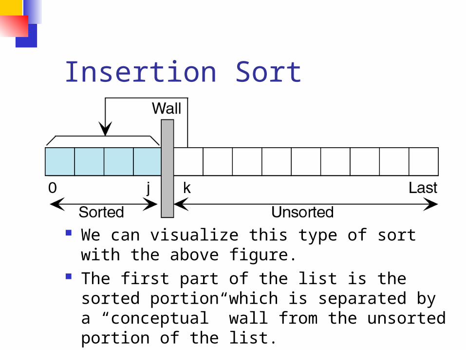
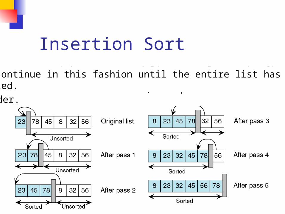
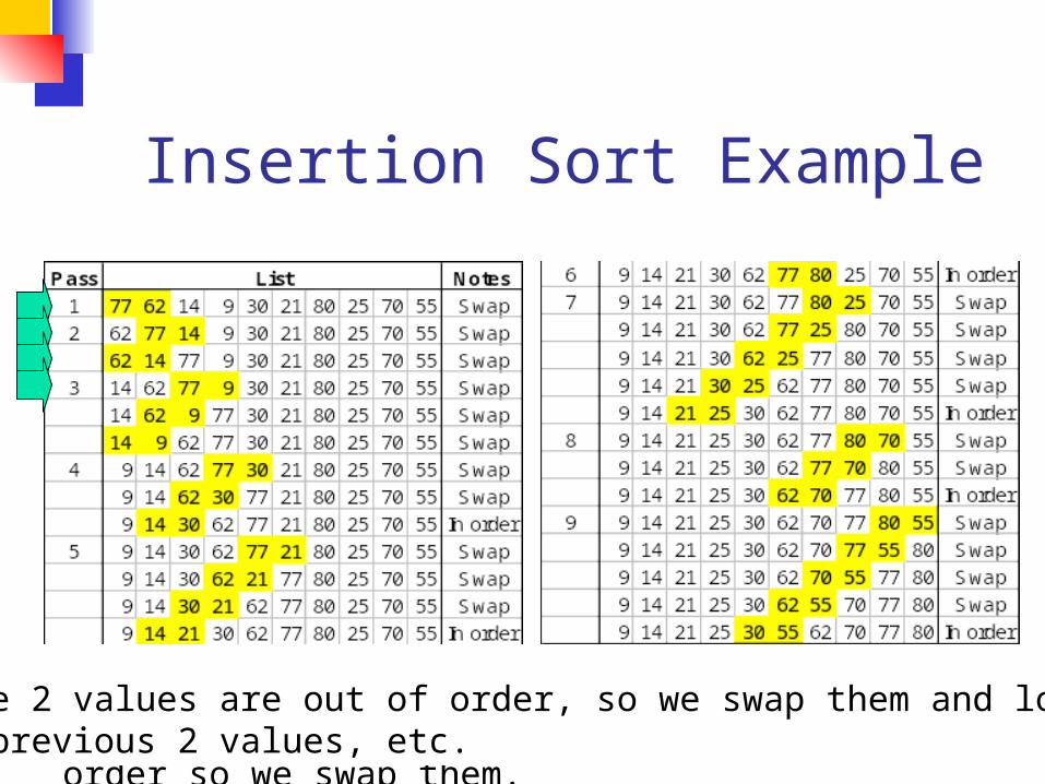
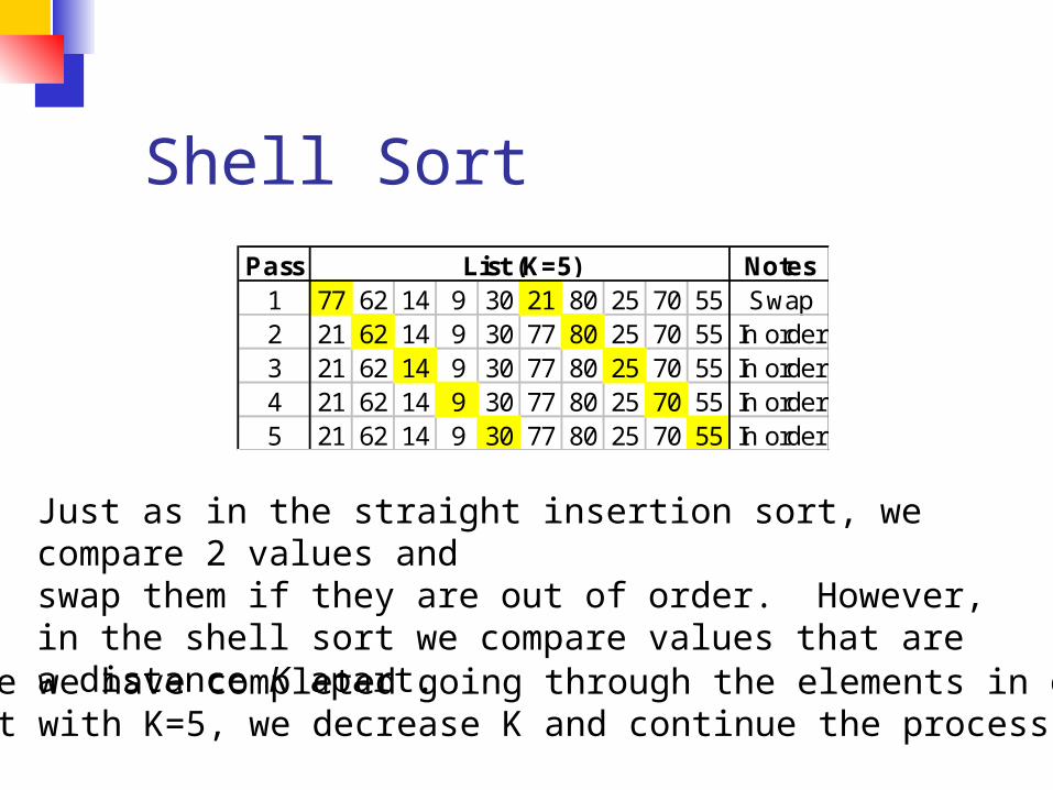
Shell SortPass Notes
1 77 62 14 9 30 21 80 25 70 55 Swap2 21 62 14 9 30 77 80 25 70 55 In order3 21 62 14 9 30 77 80 25 70 55 In order4 21 62 14 9 30 77 80 25 70 55 In order5 21 62 14 9 30 77 80 25 70 55 In order
List (K=5)
Just as in the straight insertion sort we compare 2 values andswap them if they are out of order However in the shell sort we compare values that are a distance K apartOnce we have completed going through the elements in our
list with K=5 we decrease K and continue the process
Shell SortPass Notes
6 21 62 14 9 30 77 80 25 70 55 Swap7 14 62 21 9 30 77 80 25 70 55 Swap8 14 9 21 62 30 77 80 25 70 55 In order9 14 9 21 62 30 77 80 25 70 55 In order10 14 9 21 62 30 77 80 25 70 55 In order11 14 9 21 62 30 77 80 25 70 55 Swap
14 9 21 62 30 25 80 77 70 55 Swap14 9 21 25 30 62 80 77 70 55 In order
12 14 9 21 25 30 62 80 77 70 55 Swap14 9 21 25 30 62 70 77 80 55 In order
13 14 9 21 25 30 62 70 77 80 55 Swap14 9 21 25 30 62 70 55 80 77 Swap14 9 21 25 30 55 70 62 80 77 In order
List (K=2)
Here we have reduced K to 2 Just as in the insertion sort if we swap 2 values we have to go back and compare theprevious 2 values to make sure they are still in order
Shell Sort
All shell sorts will terminate by running an insertion sort(ie K=1) However using the larger values of K first has helped to sort our list so that the straight insertion sort will runfaster
Shell Sort There are many schools of thought
on what the increment should be in the shell sort
Also note that just because an increment is optimal on one list it might not be optimal for another list
Insertion Sort vs Shell Sort Comparing the Big-O notation (for the
average case) we find that Insertion O(n2) Shell O(n125) empirically determined
Although this doesnrsquot seem like much of a gain it makes a big difference as n gets large
Note that in the worst case the Shell sort has an efficiency of O(n2)
However using a special incrementing technique this worst case can be reduced to O(n15)
Insertion Sort vs Shell Sort(Average Case)
Straight Insertion Shell25 625 55100 10000 316500 250000 2364
1000 1000000 56232000 4000000 13374
Number of Loopsn
Selection Sort Imagine some data that you can examine
all at once To sort it you could select the smallest
element and put it in its place select the next smallest and put it in its place etc
For a card player this process is analogous to looking at an entire hand of cards and ordering them by selecting cards one at a time and placing them in their proper order
Selection Sort The selection sort follows this idea Given a list of data to be sorted
we simply select the smallest item and place it in a sorted list
We then repeat these steps until the list is sorted
Selection Sort In the selection sort the list at any moment
is divided into 2 sublists sorted and unsorted separated by a ldquoconceptualrdquo wall
We select the smallest element from the unsorted sublist and exchange it with the element at the beginning of the unsorted data
After each selection and exchange the wall between the 2 sublists moves ndash increasing the number of sorted elements and decreasing the number of unsorted elements
Selection Sort
We start with an unsorted list We search this list for thesmallest element We then exchange the smallest element (8)with the first element in the unsorted list (23)
Again we search the unsorted list for the smallest element We then exchange the smallest element (23) with the first element in the unsorted list (78)
This process continues until the list is fully sorted
Bubble Sort In the bubble sort the list at any
moment is divided into 2 sublists sorted and unsorted
The smallest element is ldquobubbledrdquo from the unsorted sublist to the sorted sublist
Bubble Sort
23 78 45 8 56 3232 56
We start with 32 and compareit with 56 Because 32 is lessthan 56 we swap the twoand step down one element
We then compare 32 and 8Because 32 is not less than 8we do not swap these elements
We step down one element andcompare 45 and 8 They areout of sequence so we swapthem and step down again
8 45
We step down again and compare 8 with 78 These two elements are swapped
8 78
Finally 8 is compared with 23and swapped We thencontinue this process back with56 hellip
8 23
1 Pass of the Bubble Sort
Quick Sort In the bubble sort consecutive items
are compared and possibly exchanged on each pass through the list
This means that many exchanges may be needed to move an element to its correct position
Quick sort is more efficient than bubble sort because a typical exchange involves elements that are far apart so fewer exchanges are required to correctly position an element
Idea of Quick Sort1) Select pick an element
2) Divide rearrange elements so that x goes to its final position E
3) Recurse and Conquer recursively sort
Quick Sort Each iteration of the quick sort
selects an element known as the pivot and divides the list into 3 groups Elements whose keys are less than (or
equal to) the pivotrsquos key The pivot element Elements whose keys are greater than
(or equal to) the pivotrsquos key
Quick Sort The sorting then continues by
quick sorting the left partition followed by quick sorting the right partition
The basic algorithm is as follows
Quick Sort1) Partitioning Step Take an element in the
unsorted array and determine its final location in the sorted array This occurs when all values to the left of the element in the array are less than (or equal to) the element and all values to the right of the element are greater than (or equal to) the element We now have 1 element in its proper location and two unsorted subarrays
2) Recursive Step Perform step 1 on each unsorted subarray
Quick Sort Each time step 1 is performed on a
subarray another element is placed in its final location of the sorted array and two unsorted subarrays are created
When a subarray consists of one element that subarray is sorted
Therefore that element is in its final location
Quick Sort There are several partitioning strategies
used in practice (ie several ldquoversionsrdquo of quick sort) but the one we are about to describe is known to work well
For simplicity we will choose the last element to be the pivot element
We could also chose a different pivot element and swap it with the last element in the array
Quick Sort Below is the array we would like to
sort1 4 8 9 0 11 5 10 7 6
Quick Sort The index left starts at the first element
and right starts at the next-to-last element
We want to move all the elements smaller than the pivot to the left part of the array and all the elements larger than the pivot to the right part
1 4 8 9 0 11 5 10 7 6left righ
t
Quick Sort We move left to the right skipping
over elements that are smaller than the pivot
1 4 8 9 0 11 5 10 7 6left righ
t
Quick Sort We then move right to the left skipping
over elements that are greater than the pivot
When left and right have stopped left is on an element greater than (or equal to) the pivot and right is on an element smaller than (or equal to) the pivot
1 4 8 9 0 11 5 10 7 6left right
Quick Sort If left is to the left of right (or if left
= right) those elements are swapped
1 4 8 9 0 11 5 10 7 6left righ
t
1 4 5 9 0 11 8 10 7 6left righ
t
Quick Sort The effect is to push a large
element to the right and a small element to the left
We then repeat the process until left and right cross
Quick Sort
1 4 5 9 0 11 8 10 7 6left righ
t
1 4 5 9 0 11 8 10 7 6left righ
t
1 4 5 0 9 11 8 10 7 6left righ
t
Quick Sort
1 4 5 0 9 11 8 10 7 6left righ
t
1 4 5 0 9 11 8 10 7 6righ
tleft
Quick Sort
At this point left and right have crossed so no swap is performed
The final part of the partitioning is to swap the pivot element with left
1 4 5 0 9 11 8 10 7 6righ
tleft
1 4 5 0 6 11 8 10 7 9righ
tleft
Quick Sort Note that all elements to the left of
the pivot are less than (or equal to) the pivot and all elements to the right of the pivot are greater than (or equal to) the pivot
Hence the pivot element has been placed in its final sorted position
1 4 5 0 6 11 8 10 7 9righ
tleft
Quick Sort We now repeat the process using
the sub-arrays to the left and right of the pivot
1 4 5 0 6 11 8 10 7 9
1 4 5 0 11 8 10 7 9
Analysis of quicksortmdashbest case
Suppose each partition operation divides the array almost exactly in half
Then the depth of the recursion in log2n Because thatrsquos how many times we can
halve n However there are many recursions at
each level How can we figure this out We note that
Each partition is linear over its subarray All the partitions at one level cover the array
Partitioning at various levels
Best case II We cut the array size in half each time So the depth of the recursion in log2n At each level of the recursion all the
partitions at that level do work that is linear in n
O(log2n) O(n) = O(n log2n)
What about the worst case
Worst case In the worst case partitioning always
divides the size n array into these three parts A length one part containing the pivot itself A length zero part and A length n-1 part containing everything else
We donrsquot recur on the zero-length part Recurring on the length n-1 part requires
(in the worst case) recurring to depth n-1
Worst case partitioning
Worst case for quicksort In the worst case recursion may be
O(n) levels deep (for an array of size n)
But the partitioning work done at each level is still O(n)
O(n) O(n) = O(n2) So worst case for Quicksort is O(n2) When does this happen
When the array is sorted to begin with
Typical case for quicksort If the array is sorted to begin with
Quicksort is terrible O(n2) It is possible to construct other bad
cases However Quicksort is usually O(n log2n) The constants are so good that Quicksort
is generally the fastest algorithm known Most real-world sorting is done by
Quicksort
Tweaking Quicksort Almost anything you can try to
ldquoimproverdquo Quicksort will actually slow it down
One good tweak is to switch to a different sorting method when the subarrays get small (say 10 or 12) Quicksort has too much overhead for small
array sizes For large arrays it might be a good
idea to check beforehand if the array is already sorted But there is a better tweak than this
Randomized Quick-Sort Select the pivot as a random element of the sequence The expected running time of randomized quick-sort on a
sequence of size n is O(n log n) The time spent at a level of the quick-sort tree is O(n) We show that the expected height of the quick-sort tree is
O(log n) good vs bad pivots
bull The probability of a good pivot is 12 thus we expect k2 good pivots out of k pivotsbull After a good pivot the size of each child sequence is at most 34 the size of the parent sequencebull After h pivots we expect (34)h2 n elementsbull The expected height h of the quick-sort tree is at most 2 log43n
Median of three Obviously it doesnrsquot make sense to sort the
array in order to find the median to use as a pivot
Instead compare just three elements of our (sub)arraymdashthe first the last and the middle Take the median (middle value) of these three as
pivot Itrsquos possible (but not easy) to construct cases
which will make this technique O(n2) Suppose we rearrange (sort) these three
numbers so that the smallest is in the first position the largest in the last position and the other in the middle This lets us simplify and speed up the partition
loop
Final comments Weissrsquos code shows some additional
optimizations on pp 246-247 Weiss chooses to stop both searches on
equality to pivot This design decision is debatable
Quicksort is the fastest known general sorting algorithm on average
For optimum speed the pivot must be chosen carefully
ldquoMedian of threerdquo is a good technique for choosing the pivot
There will be some cases where Quicksort runs in O(n2) time
Quick Sort A couple of notes about quick sort There are more optimal ways to
choose the pivot value (such as the median-of-three method)
Also when the subarrays get small it becomes more efficient to use the insertion sort as opposed to continued use of quick sort
Bubble Sort vs Quick Sort If we calculate the Big-O notation
we find that (in the average case) Bubble Sort O(n2) Quick Sort O(nlog2n)
(quick-sort runs in time O(n2) in the worst case)
Heap Sort Idea take the items that need to be
sorted and insert them into the heap By calling deleteHeap we remove the
smallest or largest element depending on whether or not we are working with a min- or max-heap respectively
Hence the elements are removed in ascending or descending order
Efficiency O(nlog2n)
Merge Sort Idea
Take the array you would like to sort and divide it in half to create 2 unsorted subarrays
Next sort each of the 2 subarrays Finally merge the 2 sorted subarrays
into 1 sorted array Efficiency O(nlog2n)
Merge Sort
Merge Sort Although the merge step produces
a sorted array we have overlooked a very important step
How did we sort the 2 halves before performing the merge step
We used merge sort
Merge Sort By continually calling the merge
sort algorithm we eventually get a subarray of size 1
Since an array with only 1 element is clearly sorted we can back out and merge 2 arrays of size 1
Merge Sort
Merge Sort The basic merging algorithm
consists of 2 input arrays (arrayA and arrayB) An ouput array (arrayC) 3 position holders (indexA indexB
indexC) which are initially set to the beginning of their respective arrays
Merge Sort The smaller of arrayA[indexA] and
arrayB[indexB] is copied into arrayC[indexC] and the appropriate position holders are advanced
When either input list is exhausted the remainder of the other list is copied into arrayC
Merge Sort
1 13 24 26index
A
indexC
arrayA
2 15 27 38index
B
arrayB
arrayC
We compare arrayA[indexA]with arrayB[indexB] Whichever value is smaller isplaced into arrayC[indexC]
1 lt 2 so we insert arrayA[indexA] intoarrayC[indexC]
Merge Sort
1 13 24 26indexA
1index
C
arrayA
2 15 27 38index
B
arrayB
arrayC
2 lt 13 so we insert arrayB[indexB] intoarrayC[indexC]
Merge Sort
1 13 24 26indexA
1 2index
C
arrayA
2 15 27 38indexB
arrayB
arrayC
13 lt 15 so we insert arrayA[indexA] intoarrayC[indexC]
Merge Sort
1 13 24 26indexA
1 2 13index
C
arrayA
2 15 27 38indexB
arrayB
arrayC
15 lt 24 so we insert arrayB[indexB] intoarrayC[indexC]
Merge Sort
1 13 24 26indexA
1 2 13 15indexC
arrayA
2 15 27 38indexB
arrayB
arrayC
24 lt 27 so we insert arrayA[indexA] intoarrayC[indexC]
Merge Sort
1 13 24
26
indexA
1 2 13 15 24indexC
arrayA
2 15 27 38indexB
arrayB
arrayC
26 lt 27 so we insert arrayA[indexA] intoarrayC[indexC]
Merge Sort
1 13 24
26
1 2 13 15 24 26indexC
arrayA
2 15 27 38indexB
arrayB
arrayC
Since we have exhaustedone of the arrays arrayAwe simply copy the remaining items from theother array arrayB intoarrayC
Merge Sort
1 13 24
26
1 2 13 15 24 26 27 38
arrayA
2 15 27 38arrayB
arrayC
Efficiency Summary
Sort Worst Case Average Case
Insertion O(n2) O(n2)
Shell O(n15) O(n125)
Selection O(n2) O(n2)
Bubble O(n2) O(n2)
Quick O(n2) O(nlog2n)
Heap O(nlog2n) O(nlog2n)
Merge O(nlog2n) O(nlog2n)
More Sorting
radix sort bucket sort in-place sorting how fast can we sort
Radix Sort
Unlike other sorting methods radix sort considers the structure of the keys
Assume keys are represented in a base M number system (M = radix) ie if M = 2 the keys are represented in binary
Sorting is done by comparing bits in the same position
Extension to keys that are alphanumeric strings
Radix Exchange Sort
Examine bits from left to right1 Sort array with respect to leftmost bit
2 Partition array
3Recursionrecursively sort top subarray ignoring leftmost bitrecursively sort bottom subarray ignoring leftmost bit
Time to sort n b-bit numbers O(b n)
Radix Exchange SortHow do we do the sort from the previous page Same idea as partition in Quicksort repeat
scan top-down to find key starting with 1scan bottom-up to find key starting with 0exchange keys
until scan indices cross
Radix Exchange Sort
Radix Exchange Sort vs Quicksort
Similaritiesboth partition arrayboth recursively sort sub-arrays
DifferencesMethod of partitioning
radix exchange divides array based on greater than or less than 2b-1
quicksort partitions based on greater than or less than some element of the array
Time complexityRadix exchange O (bn)Quicksort average case O (n log n)
Straight Radix Sort
Examines bits from right to left
for k = 0 to b-1 sort the array in a stable waylooking only at bit k
Note order of these bits after sort
Recall ldquosort in a stable
wayrdquo
In a stable sort the initial relative order of equal keys is unchangedFor example observe the first step of the sort from the previous page
Note that the relative order of those keys ending with 0 is unchanged and the same is true for elements ending in 1
The Algorithm is Correct (right)
We show that any two keys are in the correct relative order at the end of the algorithm
Given two keys let k be the leftmost bit-position where they differ
At step k the two keys are put in the correct relative orderBecause of stability the successive steps do not change the relative order of the two keys
For InstanceConsider a sort on an array with these two keys
Radix sorting can be applied to decimal numbers
Straight Radix SortTime Complexity
for k = 0 to b - 1 sort the array in a stable way looking only at bit k
Suppose we can perform the stable sort above in O(n) time The total time complexity would be
O(bn)As you might have guessed we can perform a stable sort based on the keysrsquo kth digit in O(n) time
The method you ask Why itrsquos Bucket Sort of course
Bucket Sort
BASICSn numbersEach number 1 2 3 mStableTime O (n + m)
For example m = 3 and our array is
(note that there are two ldquo2rdquos and two ldquo1rdquos)
First we create M ldquobucketsrdquo
Bucket SortEach element of the array is put in one of the m ldquobucketsrdquo
Bucket Sort
Now pull the elements from the buckets into the array
At last the sorted array (sorted in a stable way)
Comparison Sorting Elements are rearranged by comparing
values of keys Comparison of keys is interleaved with
rearrangements of the order of various pairs of keys as the algorithm progressively moves keys into final sorted order
Comparisons performed at given stage will depend on outcomes of previous comparisons and previous rearrangements of keys
Sorting an array of 3 elements a b and c produces 6 or 3 distinct orderings
Decision TreeConsider a decision tree that sorts n items The next slide shows a decision tree for 3 items a b c
Ovals represent comparisons If lt we traverse down a left branch
otherwise a right branch
Decision Tree on 3 Elements
a b c
bltc
bltc
altb
altc altc
a c b b a cc a b
c b a
b c a
true
true
true true
true
false
false
false
false
false
Levels in Decision Trees Number the levels starting at zero Level i can represent 2i arrangements Our decision tree can represent 8 = 23
arrangements If we have 4 items then 4 = 24 elements
but 4 levels gives at most 24 = 16 so we need 5 levels since 25 = 32 24
If we have k arrangements to represent then we need a decision tree with at least lg k levels
Size of Decision TreeWhen dealing with n elements we have n
possible arrangements and need a decision tree with at least lg n levels
)lg(2
lg2
2lg
2
)2lg()1lg(lg
)1lg()2lg()2lg()1lg(lg
))1)(2)(2)(1(lg()lg(
nn
nn
n
nn
nnn
nnn
nnnn
Lower Bound Resultn = n(n-1)(n-2)hellip21
from this we getlg(n) = lg(n) + lg(n-1) + lg(n-2) +hellip+
lg2 + lg1this means
lg(n) lt nlg(n)and the two results together show
O(lg(n)) = O(nlg(n))
No general sorting algorithm can run faster than O(n lg n)
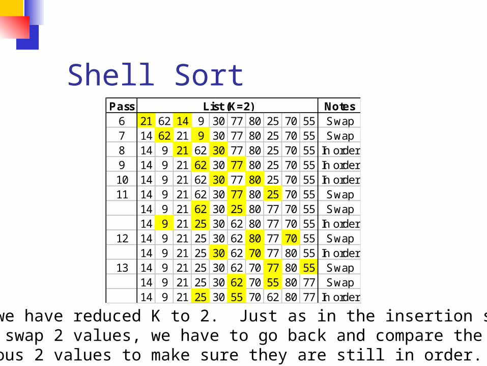
Shell SortPass Notes
6 21 62 14 9 30 77 80 25 70 55 Swap7 14 62 21 9 30 77 80 25 70 55 Swap8 14 9 21 62 30 77 80 25 70 55 In order9 14 9 21 62 30 77 80 25 70 55 In order10 14 9 21 62 30 77 80 25 70 55 In order11 14 9 21 62 30 77 80 25 70 55 Swap
14 9 21 62 30 25 80 77 70 55 Swap14 9 21 25 30 62 80 77 70 55 In order
12 14 9 21 25 30 62 80 77 70 55 Swap14 9 21 25 30 62 70 77 80 55 In order
13 14 9 21 25 30 62 70 77 80 55 Swap14 9 21 25 30 62 70 55 80 77 Swap14 9 21 25 30 55 70 62 80 77 In order
List (K=2)
Here we have reduced K to 2 Just as in the insertion sort if we swap 2 values we have to go back and compare theprevious 2 values to make sure they are still in order
Shell Sort
All shell sorts will terminate by running an insertion sort(ie K=1) However using the larger values of K first has helped to sort our list so that the straight insertion sort will runfaster
Shell Sort There are many schools of thought
on what the increment should be in the shell sort
Also note that just because an increment is optimal on one list it might not be optimal for another list
Insertion Sort vs Shell Sort Comparing the Big-O notation (for the
average case) we find that Insertion O(n2) Shell O(n125) empirically determined
Although this doesnrsquot seem like much of a gain it makes a big difference as n gets large
Note that in the worst case the Shell sort has an efficiency of O(n2)
However using a special incrementing technique this worst case can be reduced to O(n15)
Insertion Sort vs Shell Sort(Average Case)
Straight Insertion Shell25 625 55100 10000 316500 250000 2364
1000 1000000 56232000 4000000 13374
Number of Loopsn
Selection Sort Imagine some data that you can examine
all at once To sort it you could select the smallest
element and put it in its place select the next smallest and put it in its place etc
For a card player this process is analogous to looking at an entire hand of cards and ordering them by selecting cards one at a time and placing them in their proper order
Selection Sort The selection sort follows this idea Given a list of data to be sorted
we simply select the smallest item and place it in a sorted list
We then repeat these steps until the list is sorted
Selection Sort In the selection sort the list at any moment
is divided into 2 sublists sorted and unsorted separated by a ldquoconceptualrdquo wall
We select the smallest element from the unsorted sublist and exchange it with the element at the beginning of the unsorted data
After each selection and exchange the wall between the 2 sublists moves ndash increasing the number of sorted elements and decreasing the number of unsorted elements
Selection Sort
We start with an unsorted list We search this list for thesmallest element We then exchange the smallest element (8)with the first element in the unsorted list (23)
Again we search the unsorted list for the smallest element We then exchange the smallest element (23) with the first element in the unsorted list (78)
This process continues until the list is fully sorted
Bubble Sort In the bubble sort the list at any
moment is divided into 2 sublists sorted and unsorted
The smallest element is ldquobubbledrdquo from the unsorted sublist to the sorted sublist
Bubble Sort
23 78 45 8 56 3232 56
We start with 32 and compareit with 56 Because 32 is lessthan 56 we swap the twoand step down one element
We then compare 32 and 8Because 32 is not less than 8we do not swap these elements
We step down one element andcompare 45 and 8 They areout of sequence so we swapthem and step down again
8 45
We step down again and compare 8 with 78 These two elements are swapped
8 78
Finally 8 is compared with 23and swapped We thencontinue this process back with56 hellip
8 23
1 Pass of the Bubble Sort
Quick Sort In the bubble sort consecutive items
are compared and possibly exchanged on each pass through the list
This means that many exchanges may be needed to move an element to its correct position
Quick sort is more efficient than bubble sort because a typical exchange involves elements that are far apart so fewer exchanges are required to correctly position an element
Idea of Quick Sort1) Select pick an element
2) Divide rearrange elements so that x goes to its final position E
3) Recurse and Conquer recursively sort
Quick Sort Each iteration of the quick sort
selects an element known as the pivot and divides the list into 3 groups Elements whose keys are less than (or
equal to) the pivotrsquos key The pivot element Elements whose keys are greater than
(or equal to) the pivotrsquos key
Quick Sort The sorting then continues by
quick sorting the left partition followed by quick sorting the right partition
The basic algorithm is as follows
Quick Sort1) Partitioning Step Take an element in the
unsorted array and determine its final location in the sorted array This occurs when all values to the left of the element in the array are less than (or equal to) the element and all values to the right of the element are greater than (or equal to) the element We now have 1 element in its proper location and two unsorted subarrays
2) Recursive Step Perform step 1 on each unsorted subarray
Quick Sort Each time step 1 is performed on a
subarray another element is placed in its final location of the sorted array and two unsorted subarrays are created
When a subarray consists of one element that subarray is sorted
Therefore that element is in its final location
Quick Sort There are several partitioning strategies
used in practice (ie several ldquoversionsrdquo of quick sort) but the one we are about to describe is known to work well
For simplicity we will choose the last element to be the pivot element
We could also chose a different pivot element and swap it with the last element in the array
Quick Sort Below is the array we would like to
sort1 4 8 9 0 11 5 10 7 6
Quick Sort The index left starts at the first element
and right starts at the next-to-last element
We want to move all the elements smaller than the pivot to the left part of the array and all the elements larger than the pivot to the right part
1 4 8 9 0 11 5 10 7 6left righ
t
Quick Sort We move left to the right skipping
over elements that are smaller than the pivot
1 4 8 9 0 11 5 10 7 6left righ
t
Quick Sort We then move right to the left skipping
over elements that are greater than the pivot
When left and right have stopped left is on an element greater than (or equal to) the pivot and right is on an element smaller than (or equal to) the pivot
1 4 8 9 0 11 5 10 7 6left right
Quick Sort If left is to the left of right (or if left
= right) those elements are swapped
1 4 8 9 0 11 5 10 7 6left righ
t
1 4 5 9 0 11 8 10 7 6left righ
t
Quick Sort The effect is to push a large
element to the right and a small element to the left
We then repeat the process until left and right cross
Quick Sort
1 4 5 9 0 11 8 10 7 6left righ
t
1 4 5 9 0 11 8 10 7 6left righ
t
1 4 5 0 9 11 8 10 7 6left righ
t
Quick Sort
1 4 5 0 9 11 8 10 7 6left righ
t
1 4 5 0 9 11 8 10 7 6righ
tleft
Quick Sort
At this point left and right have crossed so no swap is performed
The final part of the partitioning is to swap the pivot element with left
1 4 5 0 9 11 8 10 7 6righ
tleft
1 4 5 0 6 11 8 10 7 9righ
tleft
Quick Sort Note that all elements to the left of
the pivot are less than (or equal to) the pivot and all elements to the right of the pivot are greater than (or equal to) the pivot
Hence the pivot element has been placed in its final sorted position
1 4 5 0 6 11 8 10 7 9righ
tleft
Quick Sort We now repeat the process using
the sub-arrays to the left and right of the pivot
1 4 5 0 6 11 8 10 7 9
1 4 5 0 11 8 10 7 9
Analysis of quicksortmdashbest case
Suppose each partition operation divides the array almost exactly in half
Then the depth of the recursion in log2n Because thatrsquos how many times we can
halve n However there are many recursions at
each level How can we figure this out We note that
Each partition is linear over its subarray All the partitions at one level cover the array
Partitioning at various levels
Best case II We cut the array size in half each time So the depth of the recursion in log2n At each level of the recursion all the
partitions at that level do work that is linear in n
O(log2n) O(n) = O(n log2n)
What about the worst case
Worst case In the worst case partitioning always
divides the size n array into these three parts A length one part containing the pivot itself A length zero part and A length n-1 part containing everything else
We donrsquot recur on the zero-length part Recurring on the length n-1 part requires
(in the worst case) recurring to depth n-1
Worst case partitioning
Worst case for quicksort In the worst case recursion may be
O(n) levels deep (for an array of size n)
But the partitioning work done at each level is still O(n)
O(n) O(n) = O(n2) So worst case for Quicksort is O(n2) When does this happen
When the array is sorted to begin with
Typical case for quicksort If the array is sorted to begin with
Quicksort is terrible O(n2) It is possible to construct other bad
cases However Quicksort is usually O(n log2n) The constants are so good that Quicksort
is generally the fastest algorithm known Most real-world sorting is done by
Quicksort
Tweaking Quicksort Almost anything you can try to
ldquoimproverdquo Quicksort will actually slow it down
One good tweak is to switch to a different sorting method when the subarrays get small (say 10 or 12) Quicksort has too much overhead for small
array sizes For large arrays it might be a good
idea to check beforehand if the array is already sorted But there is a better tweak than this
Randomized Quick-Sort Select the pivot as a random element of the sequence The expected running time of randomized quick-sort on a
sequence of size n is O(n log n) The time spent at a level of the quick-sort tree is O(n) We show that the expected height of the quick-sort tree is
O(log n) good vs bad pivots
bull The probability of a good pivot is 12 thus we expect k2 good pivots out of k pivotsbull After a good pivot the size of each child sequence is at most 34 the size of the parent sequencebull After h pivots we expect (34)h2 n elementsbull The expected height h of the quick-sort tree is at most 2 log43n
Median of three Obviously it doesnrsquot make sense to sort the
array in order to find the median to use as a pivot
Instead compare just three elements of our (sub)arraymdashthe first the last and the middle Take the median (middle value) of these three as
pivot Itrsquos possible (but not easy) to construct cases
which will make this technique O(n2) Suppose we rearrange (sort) these three
numbers so that the smallest is in the first position the largest in the last position and the other in the middle This lets us simplify and speed up the partition
loop
Final comments Weissrsquos code shows some additional
optimizations on pp 246-247 Weiss chooses to stop both searches on
equality to pivot This design decision is debatable
Quicksort is the fastest known general sorting algorithm on average
For optimum speed the pivot must be chosen carefully
ldquoMedian of threerdquo is a good technique for choosing the pivot
There will be some cases where Quicksort runs in O(n2) time
Quick Sort A couple of notes about quick sort There are more optimal ways to
choose the pivot value (such as the median-of-three method)
Also when the subarrays get small it becomes more efficient to use the insertion sort as opposed to continued use of quick sort
Bubble Sort vs Quick Sort If we calculate the Big-O notation
we find that (in the average case) Bubble Sort O(n2) Quick Sort O(nlog2n)
(quick-sort runs in time O(n2) in the worst case)
Heap Sort Idea take the items that need to be
sorted and insert them into the heap By calling deleteHeap we remove the
smallest or largest element depending on whether or not we are working with a min- or max-heap respectively
Hence the elements are removed in ascending or descending order
Efficiency O(nlog2n)
Merge Sort Idea
Take the array you would like to sort and divide it in half to create 2 unsorted subarrays
Next sort each of the 2 subarrays Finally merge the 2 sorted subarrays
into 1 sorted array Efficiency O(nlog2n)
Merge Sort
Merge Sort Although the merge step produces
a sorted array we have overlooked a very important step
How did we sort the 2 halves before performing the merge step
We used merge sort
Merge Sort By continually calling the merge
sort algorithm we eventually get a subarray of size 1
Since an array with only 1 element is clearly sorted we can back out and merge 2 arrays of size 1
Merge Sort
Merge Sort The basic merging algorithm
consists of 2 input arrays (arrayA and arrayB) An ouput array (arrayC) 3 position holders (indexA indexB
indexC) which are initially set to the beginning of their respective arrays
Merge Sort The smaller of arrayA[indexA] and
arrayB[indexB] is copied into arrayC[indexC] and the appropriate position holders are advanced
When either input list is exhausted the remainder of the other list is copied into arrayC
Merge Sort
1 13 24 26index
A
indexC
arrayA
2 15 27 38index
B
arrayB
arrayC
We compare arrayA[indexA]with arrayB[indexB] Whichever value is smaller isplaced into arrayC[indexC]
1 lt 2 so we insert arrayA[indexA] intoarrayC[indexC]
Merge Sort
1 13 24 26indexA
1index
C
arrayA
2 15 27 38index
B
arrayB
arrayC
2 lt 13 so we insert arrayB[indexB] intoarrayC[indexC]
Merge Sort
1 13 24 26indexA
1 2index
C
arrayA
2 15 27 38indexB
arrayB
arrayC
13 lt 15 so we insert arrayA[indexA] intoarrayC[indexC]
Merge Sort
1 13 24 26indexA
1 2 13index
C
arrayA
2 15 27 38indexB
arrayB
arrayC
15 lt 24 so we insert arrayB[indexB] intoarrayC[indexC]
Merge Sort
1 13 24 26indexA
1 2 13 15indexC
arrayA
2 15 27 38indexB
arrayB
arrayC
24 lt 27 so we insert arrayA[indexA] intoarrayC[indexC]
Merge Sort
1 13 24
26
indexA
1 2 13 15 24indexC
arrayA
2 15 27 38indexB
arrayB
arrayC
26 lt 27 so we insert arrayA[indexA] intoarrayC[indexC]
Merge Sort
1 13 24
26
1 2 13 15 24 26indexC
arrayA
2 15 27 38indexB
arrayB
arrayC
Since we have exhaustedone of the arrays arrayAwe simply copy the remaining items from theother array arrayB intoarrayC
Merge Sort
1 13 24
26
1 2 13 15 24 26 27 38
arrayA
2 15 27 38arrayB
arrayC
Efficiency Summary
Sort Worst Case Average Case
Insertion O(n2) O(n2)
Shell O(n15) O(n125)
Selection O(n2) O(n2)
Bubble O(n2) O(n2)
Quick O(n2) O(nlog2n)
Heap O(nlog2n) O(nlog2n)
Merge O(nlog2n) O(nlog2n)
More Sorting
radix sort bucket sort in-place sorting how fast can we sort
Radix Sort
Unlike other sorting methods radix sort considers the structure of the keys
Assume keys are represented in a base M number system (M = radix) ie if M = 2 the keys are represented in binary
Sorting is done by comparing bits in the same position
Extension to keys that are alphanumeric strings
Radix Exchange Sort
Examine bits from left to right1 Sort array with respect to leftmost bit
2 Partition array
3Recursionrecursively sort top subarray ignoring leftmost bitrecursively sort bottom subarray ignoring leftmost bit
Time to sort n b-bit numbers O(b n)
Radix Exchange SortHow do we do the sort from the previous page Same idea as partition in Quicksort repeat
scan top-down to find key starting with 1scan bottom-up to find key starting with 0exchange keys
until scan indices cross
Radix Exchange Sort
Radix Exchange Sort vs Quicksort
Similaritiesboth partition arrayboth recursively sort sub-arrays
DifferencesMethod of partitioning
radix exchange divides array based on greater than or less than 2b-1
quicksort partitions based on greater than or less than some element of the array
Time complexityRadix exchange O (bn)Quicksort average case O (n log n)
Straight Radix Sort
Examines bits from right to left
for k = 0 to b-1 sort the array in a stable waylooking only at bit k
Note order of these bits after sort
Recall ldquosort in a stable
wayrdquo
In a stable sort the initial relative order of equal keys is unchangedFor example observe the first step of the sort from the previous page
Note that the relative order of those keys ending with 0 is unchanged and the same is true for elements ending in 1
The Algorithm is Correct (right)
We show that any two keys are in the correct relative order at the end of the algorithm
Given two keys let k be the leftmost bit-position where they differ
At step k the two keys are put in the correct relative orderBecause of stability the successive steps do not change the relative order of the two keys
For InstanceConsider a sort on an array with these two keys
Radix sorting can be applied to decimal numbers
Straight Radix SortTime Complexity
for k = 0 to b - 1 sort the array in a stable way looking only at bit k
Suppose we can perform the stable sort above in O(n) time The total time complexity would be
O(bn)As you might have guessed we can perform a stable sort based on the keysrsquo kth digit in O(n) time
The method you ask Why itrsquos Bucket Sort of course
Bucket Sort
BASICSn numbersEach number 1 2 3 mStableTime O (n + m)
For example m = 3 and our array is
(note that there are two ldquo2rdquos and two ldquo1rdquos)
First we create M ldquobucketsrdquo
Bucket SortEach element of the array is put in one of the m ldquobucketsrdquo
Bucket Sort
Now pull the elements from the buckets into the array
At last the sorted array (sorted in a stable way)
Comparison Sorting Elements are rearranged by comparing
values of keys Comparison of keys is interleaved with
rearrangements of the order of various pairs of keys as the algorithm progressively moves keys into final sorted order
Comparisons performed at given stage will depend on outcomes of previous comparisons and previous rearrangements of keys
Sorting an array of 3 elements a b and c produces 6 or 3 distinct orderings
Decision TreeConsider a decision tree that sorts n items The next slide shows a decision tree for 3 items a b c
Ovals represent comparisons If lt we traverse down a left branch
otherwise a right branch
Decision Tree on 3 Elements
a b c
bltc
bltc
altb
altc altc
a c b b a cc a b
c b a
b c a
true
true
true true
true
false
false
false
false
false
Levels in Decision Trees Number the levels starting at zero Level i can represent 2i arrangements Our decision tree can represent 8 = 23
arrangements If we have 4 items then 4 = 24 elements
but 4 levels gives at most 24 = 16 so we need 5 levels since 25 = 32 24
If we have k arrangements to represent then we need a decision tree with at least lg k levels
Size of Decision TreeWhen dealing with n elements we have n
possible arrangements and need a decision tree with at least lg n levels
)lg(2
lg2
2lg
2
)2lg()1lg(lg
)1lg()2lg()2lg()1lg(lg
))1)(2)(2)(1(lg()lg(
nn
nn
n
nn
nnn
nnn
nnnn
Lower Bound Resultn = n(n-1)(n-2)hellip21
from this we getlg(n) = lg(n) + lg(n-1) + lg(n-2) +hellip+
lg2 + lg1this means
lg(n) lt nlg(n)and the two results together show
O(lg(n)) = O(nlg(n))
No general sorting algorithm can run faster than O(n lg n)
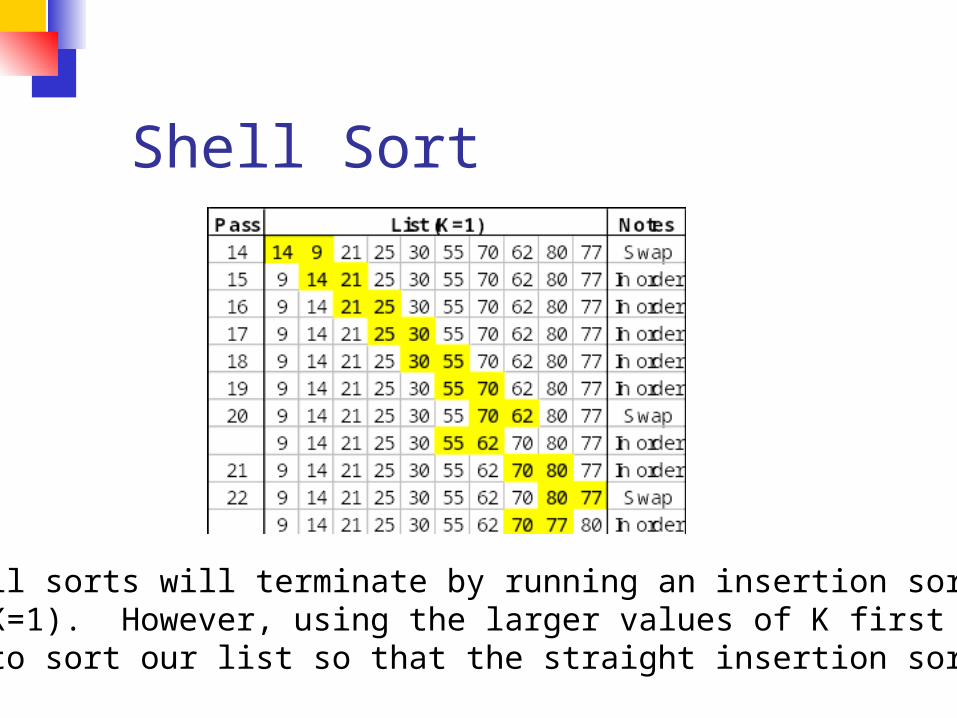
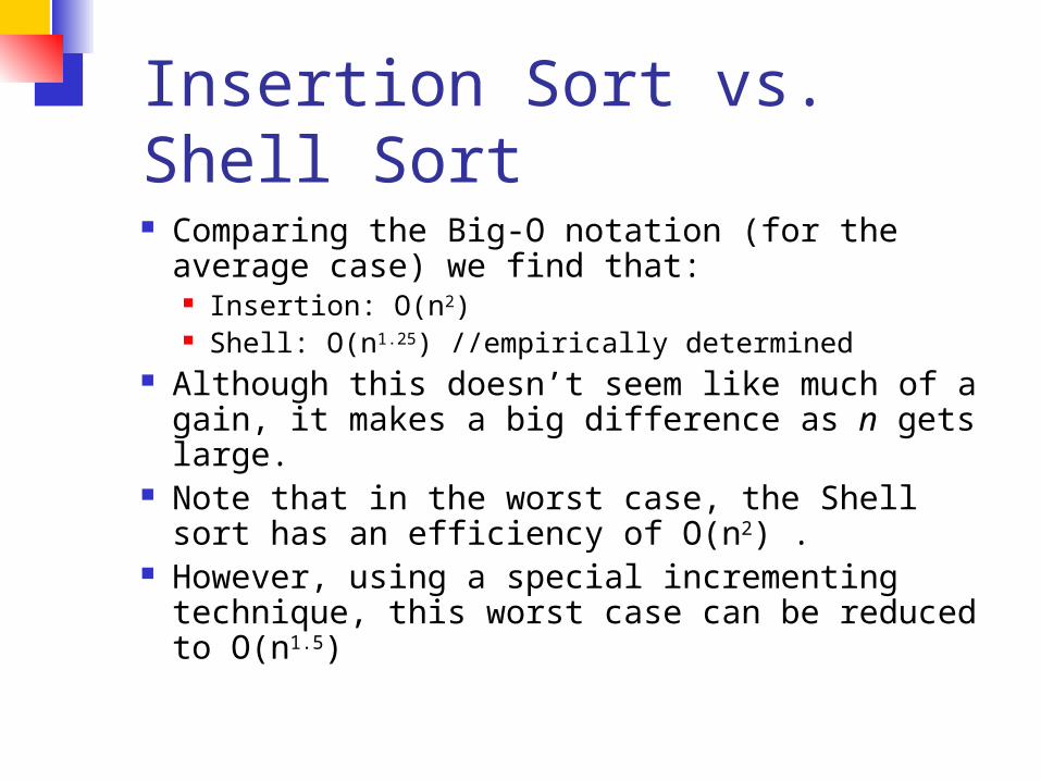
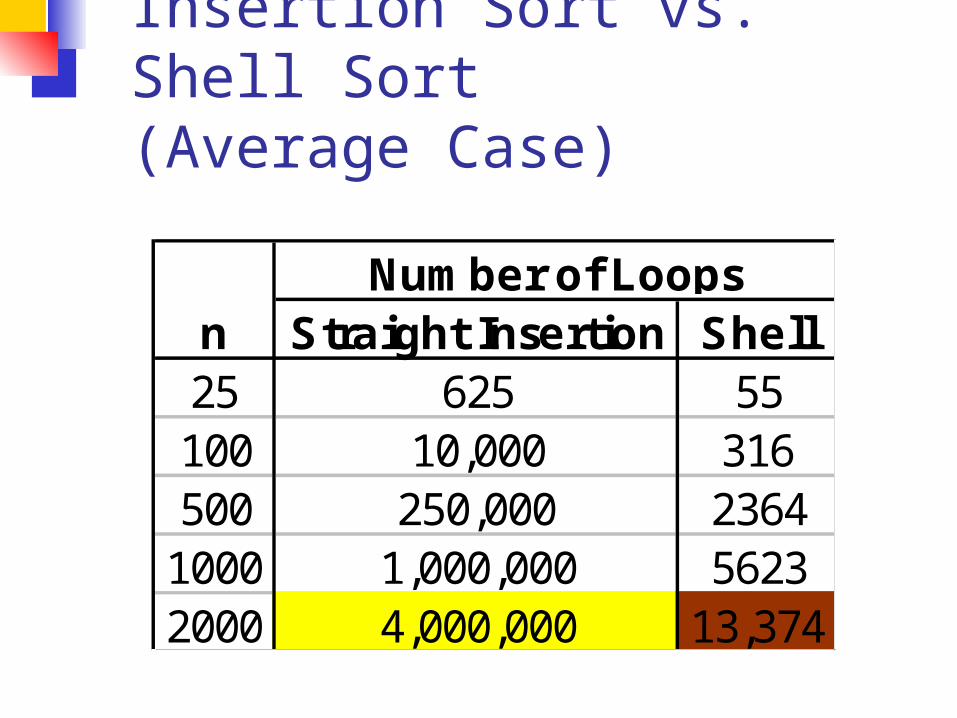
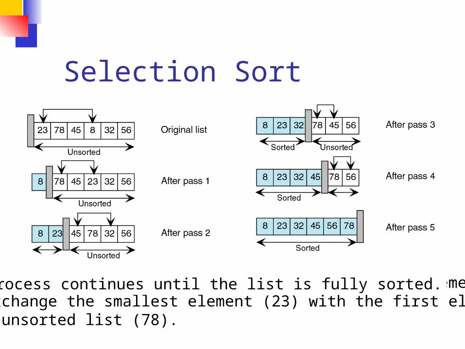
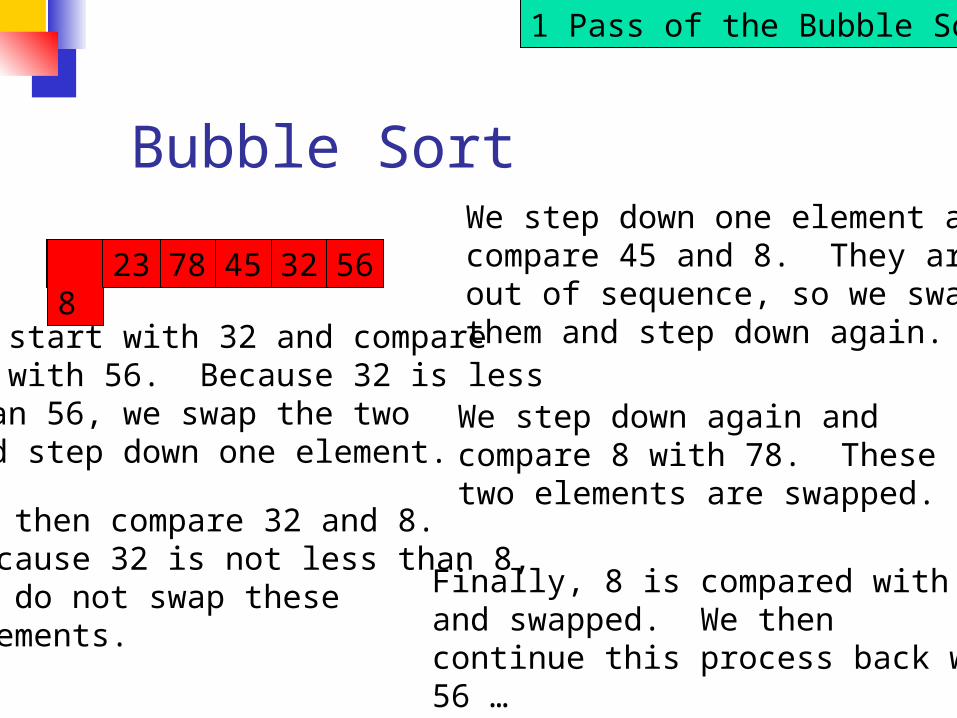
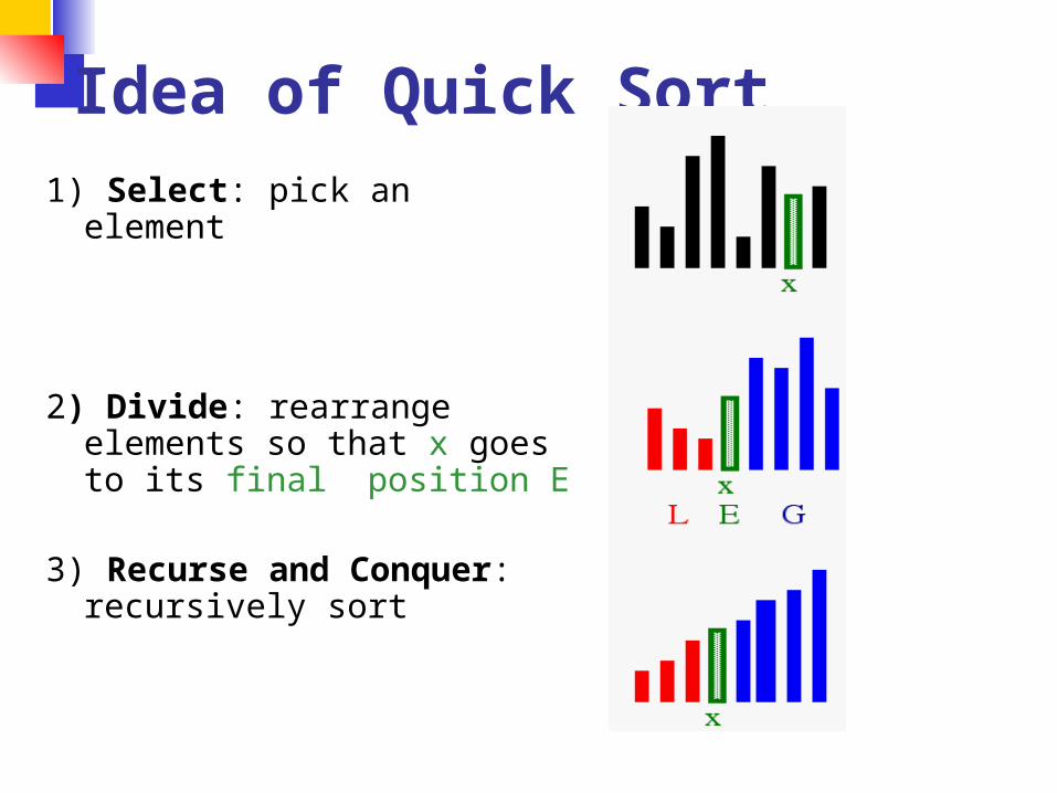
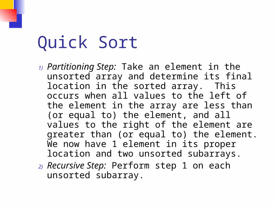
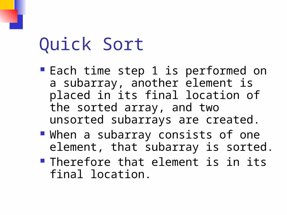
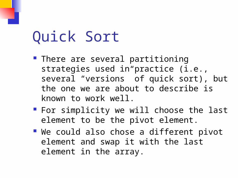
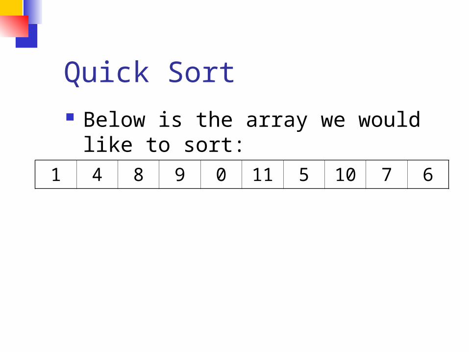
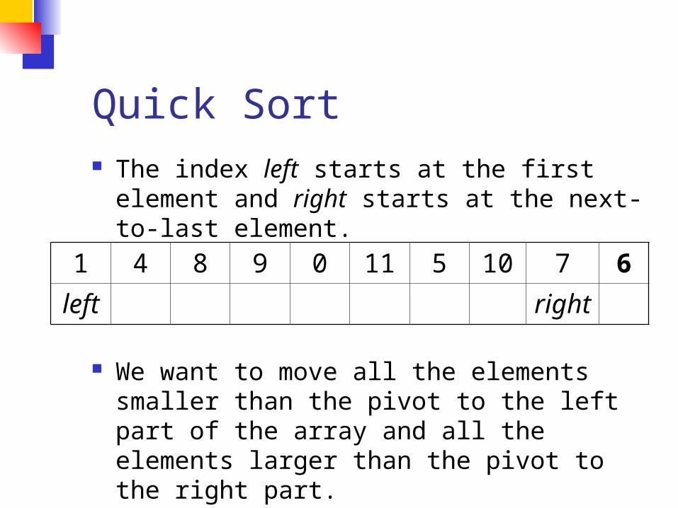
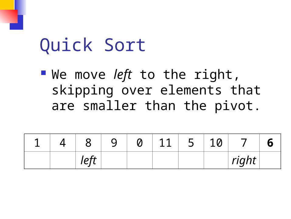
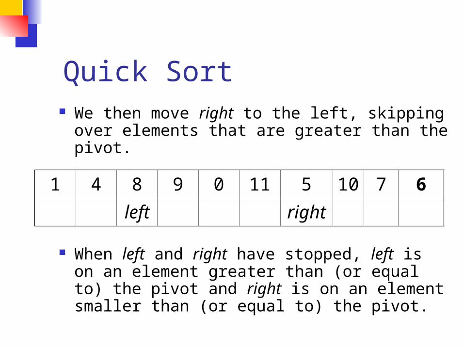
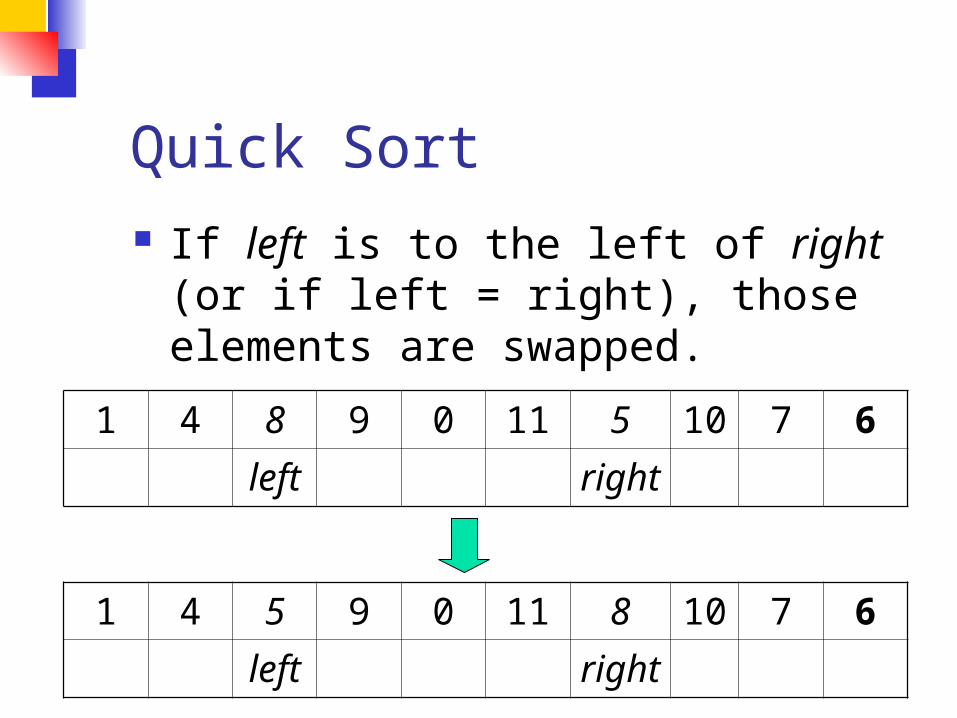
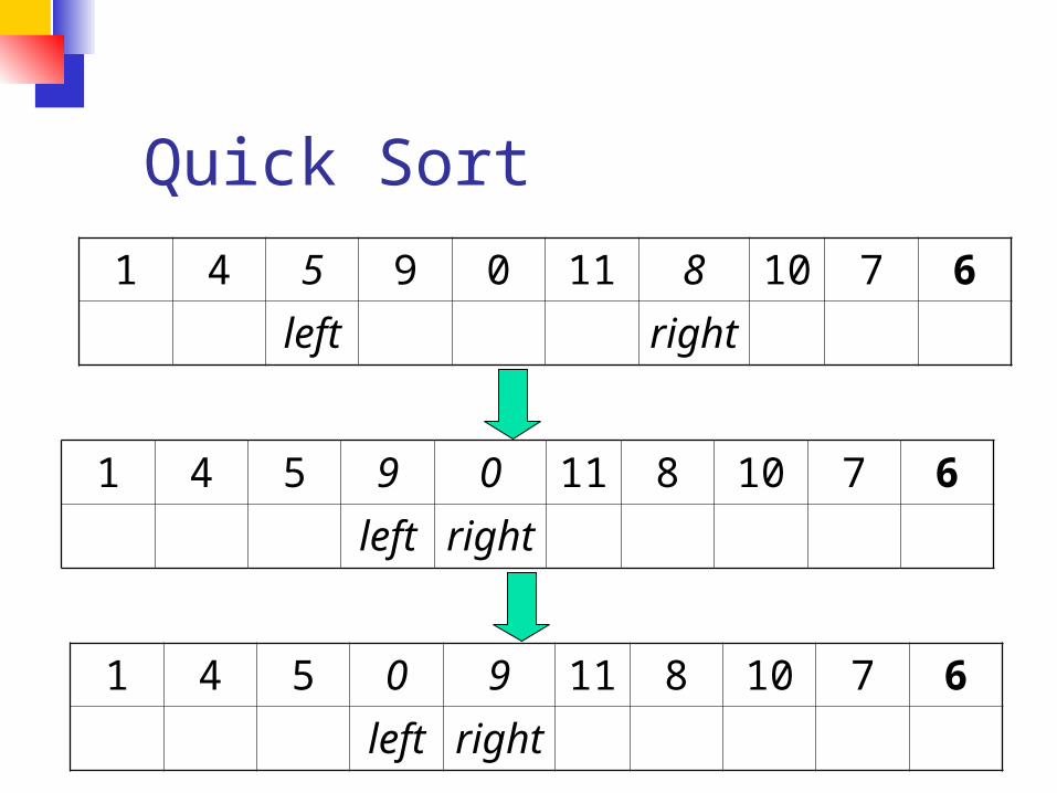
Quick Sort
1 4 5 9 0 11 8 10 7 6left righ
t
1 4 5 9 0 11 8 10 7 6left righ
t
1 4 5 0 9 11 8 10 7 6left righ
t
Quick Sort
1 4 5 0 9 11 8 10 7 6left righ
t
1 4 5 0 9 11 8 10 7 6righ
tleft
Quick Sort
At this point left and right have crossed so no swap is performed
The final part of the partitioning is to swap the pivot element with left
1 4 5 0 9 11 8 10 7 6righ
tleft
1 4 5 0 6 11 8 10 7 9righ
tleft
Quick Sort Note that all elements to the left of
the pivot are less than (or equal to) the pivot and all elements to the right of the pivot are greater than (or equal to) the pivot
Hence the pivot element has been placed in its final sorted position
1 4 5 0 6 11 8 10 7 9righ
tleft
Quick Sort We now repeat the process using
the sub-arrays to the left and right of the pivot
1 4 5 0 6 11 8 10 7 9
1 4 5 0 11 8 10 7 9
Analysis of quicksortmdashbest case
Suppose each partition operation divides the array almost exactly in half
Then the depth of the recursion in log2n Because thatrsquos how many times we can
halve n However there are many recursions at
each level How can we figure this out We note that
Each partition is linear over its subarray All the partitions at one level cover the array
Partitioning at various levels
Best case II We cut the array size in half each time So the depth of the recursion in log2n At each level of the recursion all the
partitions at that level do work that is linear in n
O(log2n) O(n) = O(n log2n)
What about the worst case
Worst case In the worst case partitioning always
divides the size n array into these three parts A length one part containing the pivot itself A length zero part and A length n-1 part containing everything else
We donrsquot recur on the zero-length part Recurring on the length n-1 part requires
(in the worst case) recurring to depth n-1
Worst case partitioning
Worst case for quicksort In the worst case recursion may be
O(n) levels deep (for an array of size n)
But the partitioning work done at each level is still O(n)
O(n) O(n) = O(n2) So worst case for Quicksort is O(n2) When does this happen
When the array is sorted to begin with
Typical case for quicksort If the array is sorted to begin with
Quicksort is terrible O(n2) It is possible to construct other bad
cases However Quicksort is usually O(n log2n) The constants are so good that Quicksort
is generally the fastest algorithm known Most real-world sorting is done by
Quicksort
Tweaking Quicksort Almost anything you can try to
ldquoimproverdquo Quicksort will actually slow it down
One good tweak is to switch to a different sorting method when the subarrays get small (say 10 or 12) Quicksort has too much overhead for small
array sizes For large arrays it might be a good
idea to check beforehand if the array is already sorted But there is a better tweak than this
Randomized Quick-Sort Select the pivot as a random element of the sequence The expected running time of randomized quick-sort on a
sequence of size n is O(n log n) The time spent at a level of the quick-sort tree is O(n) We show that the expected height of the quick-sort tree is
O(log n) good vs bad pivots
bull The probability of a good pivot is 12 thus we expect k2 good pivots out of k pivotsbull After a good pivot the size of each child sequence is at most 34 the size of the parent sequencebull After h pivots we expect (34)h2 n elementsbull The expected height h of the quick-sort tree is at most 2 log43n
Median of three Obviously it doesnrsquot make sense to sort the
array in order to find the median to use as a pivot
Instead compare just three elements of our (sub)arraymdashthe first the last and the middle Take the median (middle value) of these three as
pivot Itrsquos possible (but not easy) to construct cases
which will make this technique O(n2) Suppose we rearrange (sort) these three
numbers so that the smallest is in the first position the largest in the last position and the other in the middle This lets us simplify and speed up the partition
loop
Final comments Weissrsquos code shows some additional
optimizations on pp 246-247 Weiss chooses to stop both searches on
equality to pivot This design decision is debatable
Quicksort is the fastest known general sorting algorithm on average
For optimum speed the pivot must be chosen carefully
ldquoMedian of threerdquo is a good technique for choosing the pivot
There will be some cases where Quicksort runs in O(n2) time
Quick Sort A couple of notes about quick sort There are more optimal ways to
choose the pivot value (such as the median-of-three method)
Also when the subarrays get small it becomes more efficient to use the insertion sort as opposed to continued use of quick sort
Bubble Sort vs Quick Sort If we calculate the Big-O notation
we find that (in the average case) Bubble Sort O(n2) Quick Sort O(nlog2n)
(quick-sort runs in time O(n2) in the worst case)
Heap Sort Idea take the items that need to be
sorted and insert them into the heap By calling deleteHeap we remove the
smallest or largest element depending on whether or not we are working with a min- or max-heap respectively
Hence the elements are removed in ascending or descending order
Efficiency O(nlog2n)
Merge Sort Idea
Take the array you would like to sort and divide it in half to create 2 unsorted subarrays
Next sort each of the 2 subarrays Finally merge the 2 sorted subarrays
into 1 sorted array Efficiency O(nlog2n)
Merge Sort
Merge Sort Although the merge step produces
a sorted array we have overlooked a very important step
How did we sort the 2 halves before performing the merge step
We used merge sort
Merge Sort By continually calling the merge
sort algorithm we eventually get a subarray of size 1
Since an array with only 1 element is clearly sorted we can back out and merge 2 arrays of size 1
Merge Sort
Merge Sort The basic merging algorithm
consists of 2 input arrays (arrayA and arrayB) An ouput array (arrayC) 3 position holders (indexA indexB
indexC) which are initially set to the beginning of their respective arrays
Merge Sort The smaller of arrayA[indexA] and
arrayB[indexB] is copied into arrayC[indexC] and the appropriate position holders are advanced
When either input list is exhausted the remainder of the other list is copied into arrayC
Merge Sort
1 13 24 26index
A
indexC
arrayA
2 15 27 38index
B
arrayB
arrayC
We compare arrayA[indexA]with arrayB[indexB] Whichever value is smaller isplaced into arrayC[indexC]
1 lt 2 so we insert arrayA[indexA] intoarrayC[indexC]
Merge Sort
1 13 24 26indexA
1index
C
arrayA
2 15 27 38index
B
arrayB
arrayC
2 lt 13 so we insert arrayB[indexB] intoarrayC[indexC]
Merge Sort
1 13 24 26indexA
1 2index
C
arrayA
2 15 27 38indexB
arrayB
arrayC
13 lt 15 so we insert arrayA[indexA] intoarrayC[indexC]
Merge Sort
1 13 24 26indexA
1 2 13index
C
arrayA
2 15 27 38indexB
arrayB
arrayC
15 lt 24 so we insert arrayB[indexB] intoarrayC[indexC]
Merge Sort
1 13 24 26indexA
1 2 13 15indexC
arrayA
2 15 27 38indexB
arrayB
arrayC
24 lt 27 so we insert arrayA[indexA] intoarrayC[indexC]
Merge Sort
1 13 24
26
indexA
1 2 13 15 24indexC
arrayA
2 15 27 38indexB
arrayB
arrayC
26 lt 27 so we insert arrayA[indexA] intoarrayC[indexC]
Merge Sort
1 13 24
26
1 2 13 15 24 26indexC
arrayA
2 15 27 38indexB
arrayB
arrayC
Since we have exhaustedone of the arrays arrayAwe simply copy the remaining items from theother array arrayB intoarrayC
Merge Sort
1 13 24
26
1 2 13 15 24 26 27 38
arrayA
2 15 27 38arrayB
arrayC
Efficiency Summary
Sort Worst Case Average Case
Insertion O(n2) O(n2)
Shell O(n15) O(n125)
Selection O(n2) O(n2)
Bubble O(n2) O(n2)
Quick O(n2) O(nlog2n)
Heap O(nlog2n) O(nlog2n)
Merge O(nlog2n) O(nlog2n)
More Sorting
radix sort bucket sort in-place sorting how fast can we sort
Radix Sort
Unlike other sorting methods radix sort considers the structure of the keys
Assume keys are represented in a base M number system (M = radix) ie if M = 2 the keys are represented in binary
Sorting is done by comparing bits in the same position
Extension to keys that are alphanumeric strings
Radix Exchange Sort
Examine bits from left to right1 Sort array with respect to leftmost bit
2 Partition array
3Recursionrecursively sort top subarray ignoring leftmost bitrecursively sort bottom subarray ignoring leftmost bit
Time to sort n b-bit numbers O(b n)
Radix Exchange SortHow do we do the sort from the previous page Same idea as partition in Quicksort repeat
scan top-down to find key starting with 1scan bottom-up to find key starting with 0exchange keys
until scan indices cross
Radix Exchange Sort
Radix Exchange Sort vs Quicksort
Similaritiesboth partition arrayboth recursively sort sub-arrays
DifferencesMethod of partitioning
radix exchange divides array based on greater than or less than 2b-1
quicksort partitions based on greater than or less than some element of the array
Time complexityRadix exchange O (bn)Quicksort average case O (n log n)
Straight Radix Sort
Examines bits from right to left
for k = 0 to b-1 sort the array in a stable waylooking only at bit k
Note order of these bits after sort
Recall ldquosort in a stable
wayrdquo
In a stable sort the initial relative order of equal keys is unchangedFor example observe the first step of the sort from the previous page
Note that the relative order of those keys ending with 0 is unchanged and the same is true for elements ending in 1
The Algorithm is Correct (right)
We show that any two keys are in the correct relative order at the end of the algorithm
Given two keys let k be the leftmost bit-position where they differ
At step k the two keys are put in the correct relative orderBecause of stability the successive steps do not change the relative order of the two keys
For InstanceConsider a sort on an array with these two keys
Radix sorting can be applied to decimal numbers
Straight Radix SortTime Complexity
for k = 0 to b - 1 sort the array in a stable way looking only at bit k
Suppose we can perform the stable sort above in O(n) time The total time complexity would be
O(bn)As you might have guessed we can perform a stable sort based on the keysrsquo kth digit in O(n) time
The method you ask Why itrsquos Bucket Sort of course
Bucket Sort
BASICSn numbersEach number 1 2 3 mStableTime O (n + m)
For example m = 3 and our array is
(note that there are two ldquo2rdquos and two ldquo1rdquos)
First we create M ldquobucketsrdquo
Bucket SortEach element of the array is put in one of the m ldquobucketsrdquo
Bucket Sort
Now pull the elements from the buckets into the array
At last the sorted array (sorted in a stable way)
Comparison Sorting Elements are rearranged by comparing
values of keys Comparison of keys is interleaved with
rearrangements of the order of various pairs of keys as the algorithm progressively moves keys into final sorted order
Comparisons performed at given stage will depend on outcomes of previous comparisons and previous rearrangements of keys
Sorting an array of 3 elements a b and c produces 6 or 3 distinct orderings
Decision TreeConsider a decision tree that sorts n items The next slide shows a decision tree for 3 items a b c
Ovals represent comparisons If lt we traverse down a left branch
otherwise a right branch
Decision Tree on 3 Elements
a b c
bltc
bltc
altb
altc altc
a c b b a cc a b
c b a
b c a
true
true
true true
true
false
false
false
false
false
Levels in Decision Trees Number the levels starting at zero Level i can represent 2i arrangements Our decision tree can represent 8 = 23
arrangements If we have 4 items then 4 = 24 elements
but 4 levels gives at most 24 = 16 so we need 5 levels since 25 = 32 24
If we have k arrangements to represent then we need a decision tree with at least lg k levels
Size of Decision TreeWhen dealing with n elements we have n
possible arrangements and need a decision tree with at least lg n levels
)lg(2
lg2
2lg
2
)2lg()1lg(lg
)1lg()2lg()2lg()1lg(lg
))1)(2)(2)(1(lg()lg(
nn
nn
n
nn
nnn
nnn
nnnn
Lower Bound Resultn = n(n-1)(n-2)hellip21
from this we getlg(n) = lg(n) + lg(n-1) + lg(n-2) +hellip+
lg2 + lg1this means
lg(n) lt nlg(n)and the two results together show
O(lg(n)) = O(nlg(n))
No general sorting algorithm can run faster than O(n lg n)
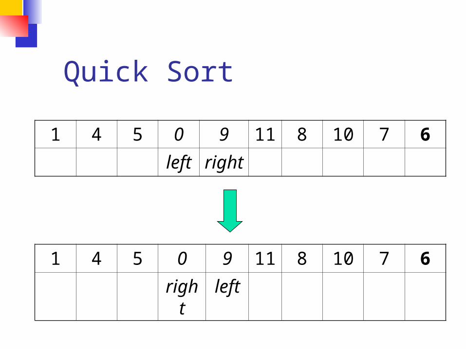
Quick Sort
1 4 5 0 9 11 8 10 7 6left righ
t
1 4 5 0 9 11 8 10 7 6righ
tleft
Quick Sort
At this point left and right have crossed so no swap is performed
The final part of the partitioning is to swap the pivot element with left
1 4 5 0 9 11 8 10 7 6righ
tleft
1 4 5 0 6 11 8 10 7 9righ
tleft
Quick Sort Note that all elements to the left of
the pivot are less than (or equal to) the pivot and all elements to the right of the pivot are greater than (or equal to) the pivot
Hence the pivot element has been placed in its final sorted position
1 4 5 0 6 11 8 10 7 9righ
tleft
Quick Sort We now repeat the process using
the sub-arrays to the left and right of the pivot
1 4 5 0 6 11 8 10 7 9
1 4 5 0 11 8 10 7 9
Analysis of quicksortmdashbest case
Suppose each partition operation divides the array almost exactly in half
Then the depth of the recursion in log2n Because thatrsquos how many times we can
halve n However there are many recursions at
each level How can we figure this out We note that
Each partition is linear over its subarray All the partitions at one level cover the array
Partitioning at various levels
Best case II We cut the array size in half each time So the depth of the recursion in log2n At each level of the recursion all the
partitions at that level do work that is linear in n
O(log2n) O(n) = O(n log2n)
What about the worst case
Worst case In the worst case partitioning always
divides the size n array into these three parts A length one part containing the pivot itself A length zero part and A length n-1 part containing everything else
We donrsquot recur on the zero-length part Recurring on the length n-1 part requires
(in the worst case) recurring to depth n-1
Worst case partitioning
Worst case for quicksort In the worst case recursion may be
O(n) levels deep (for an array of size n)
But the partitioning work done at each level is still O(n)
O(n) O(n) = O(n2) So worst case for Quicksort is O(n2) When does this happen
When the array is sorted to begin with
Typical case for quicksort If the array is sorted to begin with
Quicksort is terrible O(n2) It is possible to construct other bad
cases However Quicksort is usually O(n log2n) The constants are so good that Quicksort
is generally the fastest algorithm known Most real-world sorting is done by
Quicksort
Tweaking Quicksort Almost anything you can try to
ldquoimproverdquo Quicksort will actually slow it down
One good tweak is to switch to a different sorting method when the subarrays get small (say 10 or 12) Quicksort has too much overhead for small
array sizes For large arrays it might be a good
idea to check beforehand if the array is already sorted But there is a better tweak than this
Randomized Quick-Sort Select the pivot as a random element of the sequence The expected running time of randomized quick-sort on a
sequence of size n is O(n log n) The time spent at a level of the quick-sort tree is O(n) We show that the expected height of the quick-sort tree is
O(log n) good vs bad pivots
bull The probability of a good pivot is 12 thus we expect k2 good pivots out of k pivotsbull After a good pivot the size of each child sequence is at most 34 the size of the parent sequencebull After h pivots we expect (34)h2 n elementsbull The expected height h of the quick-sort tree is at most 2 log43n
Median of three Obviously it doesnrsquot make sense to sort the
array in order to find the median to use as a pivot
Instead compare just three elements of our (sub)arraymdashthe first the last and the middle Take the median (middle value) of these three as
pivot Itrsquos possible (but not easy) to construct cases
which will make this technique O(n2) Suppose we rearrange (sort) these three
numbers so that the smallest is in the first position the largest in the last position and the other in the middle This lets us simplify and speed up the partition
loop
Final comments Weissrsquos code shows some additional
optimizations on pp 246-247 Weiss chooses to stop both searches on
equality to pivot This design decision is debatable
Quicksort is the fastest known general sorting algorithm on average
For optimum speed the pivot must be chosen carefully
ldquoMedian of threerdquo is a good technique for choosing the pivot
There will be some cases where Quicksort runs in O(n2) time
Quick Sort A couple of notes about quick sort There are more optimal ways to
choose the pivot value (such as the median-of-three method)
Also when the subarrays get small it becomes more efficient to use the insertion sort as opposed to continued use of quick sort
Bubble Sort vs Quick Sort If we calculate the Big-O notation
we find that (in the average case) Bubble Sort O(n2) Quick Sort O(nlog2n)
(quick-sort runs in time O(n2) in the worst case)
Heap Sort Idea take the items that need to be
sorted and insert them into the heap By calling deleteHeap we remove the
smallest or largest element depending on whether or not we are working with a min- or max-heap respectively
Hence the elements are removed in ascending or descending order
Efficiency O(nlog2n)
Merge Sort Idea
Take the array you would like to sort and divide it in half to create 2 unsorted subarrays
Next sort each of the 2 subarrays Finally merge the 2 sorted subarrays
into 1 sorted array Efficiency O(nlog2n)
Merge Sort
Merge Sort Although the merge step produces
a sorted array we have overlooked a very important step
How did we sort the 2 halves before performing the merge step
We used merge sort
Merge Sort By continually calling the merge
sort algorithm we eventually get a subarray of size 1
Since an array with only 1 element is clearly sorted we can back out and merge 2 arrays of size 1
Merge Sort
Merge Sort The basic merging algorithm
consists of 2 input arrays (arrayA and arrayB) An ouput array (arrayC) 3 position holders (indexA indexB
indexC) which are initially set to the beginning of their respective arrays
Merge Sort The smaller of arrayA[indexA] and
arrayB[indexB] is copied into arrayC[indexC] and the appropriate position holders are advanced
When either input list is exhausted the remainder of the other list is copied into arrayC
Merge Sort
1 13 24 26index
A
indexC
arrayA
2 15 27 38index
B
arrayB
arrayC
We compare arrayA[indexA]with arrayB[indexB] Whichever value is smaller isplaced into arrayC[indexC]
1 lt 2 so we insert arrayA[indexA] intoarrayC[indexC]
Merge Sort
1 13 24 26indexA
1index
C
arrayA
2 15 27 38index
B
arrayB
arrayC
2 lt 13 so we insert arrayB[indexB] intoarrayC[indexC]
Merge Sort
1 13 24 26indexA
1 2index
C
arrayA
2 15 27 38indexB
arrayB
arrayC
13 lt 15 so we insert arrayA[indexA] intoarrayC[indexC]
Merge Sort
1 13 24 26indexA
1 2 13index
C
arrayA
2 15 27 38indexB
arrayB
arrayC
15 lt 24 so we insert arrayB[indexB] intoarrayC[indexC]
Merge Sort
1 13 24 26indexA
1 2 13 15indexC
arrayA
2 15 27 38indexB
arrayB
arrayC
24 lt 27 so we insert arrayA[indexA] intoarrayC[indexC]
Merge Sort
1 13 24
26
indexA
1 2 13 15 24indexC
arrayA
2 15 27 38indexB
arrayB
arrayC
26 lt 27 so we insert arrayA[indexA] intoarrayC[indexC]
Merge Sort
1 13 24
26
1 2 13 15 24 26indexC
arrayA
2 15 27 38indexB
arrayB
arrayC
Since we have exhaustedone of the arrays arrayAwe simply copy the remaining items from theother array arrayB intoarrayC
Merge Sort
1 13 24
26
1 2 13 15 24 26 27 38
arrayA
2 15 27 38arrayB
arrayC
Efficiency Summary
Sort Worst Case Average Case
Insertion O(n2) O(n2)
Shell O(n15) O(n125)
Selection O(n2) O(n2)
Bubble O(n2) O(n2)
Quick O(n2) O(nlog2n)
Heap O(nlog2n) O(nlog2n)
Merge O(nlog2n) O(nlog2n)
More Sorting
radix sort bucket sort in-place sorting how fast can we sort
Radix Sort
Unlike other sorting methods radix sort considers the structure of the keys
Assume keys are represented in a base M number system (M = radix) ie if M = 2 the keys are represented in binary
Sorting is done by comparing bits in the same position
Extension to keys that are alphanumeric strings
Radix Exchange Sort
Examine bits from left to right1 Sort array with respect to leftmost bit
2 Partition array
3Recursionrecursively sort top subarray ignoring leftmost bitrecursively sort bottom subarray ignoring leftmost bit
Time to sort n b-bit numbers O(b n)
Radix Exchange SortHow do we do the sort from the previous page Same idea as partition in Quicksort repeat
scan top-down to find key starting with 1scan bottom-up to find key starting with 0exchange keys
until scan indices cross
Radix Exchange Sort
Radix Exchange Sort vs Quicksort
Similaritiesboth partition arrayboth recursively sort sub-arrays
DifferencesMethod of partitioning
radix exchange divides array based on greater than or less than 2b-1
quicksort partitions based on greater than or less than some element of the array
Time complexityRadix exchange O (bn)Quicksort average case O (n log n)
Straight Radix Sort
Examines bits from right to left
for k = 0 to b-1 sort the array in a stable waylooking only at bit k
Note order of these bits after sort
Recall ldquosort in a stable
wayrdquo
In a stable sort the initial relative order of equal keys is unchangedFor example observe the first step of the sort from the previous page
Note that the relative order of those keys ending with 0 is unchanged and the same is true for elements ending in 1
The Algorithm is Correct (right)
We show that any two keys are in the correct relative order at the end of the algorithm
Given two keys let k be the leftmost bit-position where they differ
At step k the two keys are put in the correct relative orderBecause of stability the successive steps do not change the relative order of the two keys
For InstanceConsider a sort on an array with these two keys
Radix sorting can be applied to decimal numbers
Straight Radix SortTime Complexity
for k = 0 to b - 1 sort the array in a stable way looking only at bit k
Suppose we can perform the stable sort above in O(n) time The total time complexity would be
O(bn)As you might have guessed we can perform a stable sort based on the keysrsquo kth digit in O(n) time
The method you ask Why itrsquos Bucket Sort of course
Bucket Sort
BASICSn numbersEach number 1 2 3 mStableTime O (n + m)
For example m = 3 and our array is
(note that there are two ldquo2rdquos and two ldquo1rdquos)
First we create M ldquobucketsrdquo
Bucket SortEach element of the array is put in one of the m ldquobucketsrdquo
Bucket Sort
Now pull the elements from the buckets into the array
At last the sorted array (sorted in a stable way)
Comparison Sorting Elements are rearranged by comparing
values of keys Comparison of keys is interleaved with
rearrangements of the order of various pairs of keys as the algorithm progressively moves keys into final sorted order
Comparisons performed at given stage will depend on outcomes of previous comparisons and previous rearrangements of keys
Sorting an array of 3 elements a b and c produces 6 or 3 distinct orderings
Decision TreeConsider a decision tree that sorts n items The next slide shows a decision tree for 3 items a b c
Ovals represent comparisons If lt we traverse down a left branch
otherwise a right branch
Decision Tree on 3 Elements
a b c
bltc
bltc
altb
altc altc
a c b b a cc a b
c b a
b c a
true
true
true true
true
false
false
false
false
false
Levels in Decision Trees Number the levels starting at zero Level i can represent 2i arrangements Our decision tree can represent 8 = 23
arrangements If we have 4 items then 4 = 24 elements
but 4 levels gives at most 24 = 16 so we need 5 levels since 25 = 32 24
If we have k arrangements to represent then we need a decision tree with at least lg k levels
Size of Decision TreeWhen dealing with n elements we have n
possible arrangements and need a decision tree with at least lg n levels
)lg(2
lg2
2lg
2
)2lg()1lg(lg
)1lg()2lg()2lg()1lg(lg
))1)(2)(2)(1(lg()lg(
nn
nn
n
nn
nnn
nnn
nnnn
Lower Bound Resultn = n(n-1)(n-2)hellip21
from this we getlg(n) = lg(n) + lg(n-1) + lg(n-2) +hellip+
lg2 + lg1this means
lg(n) lt nlg(n)and the two results together show
O(lg(n)) = O(nlg(n))
No general sorting algorithm can run faster than O(n lg n)
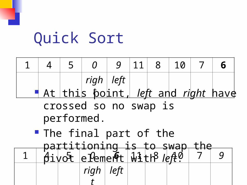
Quick Sort
At this point left and right have crossed so no swap is performed
The final part of the partitioning is to swap the pivot element with left
1 4 5 0 9 11 8 10 7 6righ
tleft
1 4 5 0 6 11 8 10 7 9righ
tleft
Quick Sort Note that all elements to the left of
the pivot are less than (or equal to) the pivot and all elements to the right of the pivot are greater than (or equal to) the pivot
Hence the pivot element has been placed in its final sorted position
1 4 5 0 6 11 8 10 7 9righ
tleft
Quick Sort We now repeat the process using
the sub-arrays to the left and right of the pivot
1 4 5 0 6 11 8 10 7 9
1 4 5 0 11 8 10 7 9
Analysis of quicksortmdashbest case
Suppose each partition operation divides the array almost exactly in half
Then the depth of the recursion in log2n Because thatrsquos how many times we can
halve n However there are many recursions at
each level How can we figure this out We note that
Each partition is linear over its subarray All the partitions at one level cover the array
Partitioning at various levels
Best case II We cut the array size in half each time So the depth of the recursion in log2n At each level of the recursion all the
partitions at that level do work that is linear in n
O(log2n) O(n) = O(n log2n)
What about the worst case
Worst case In the worst case partitioning always
divides the size n array into these three parts A length one part containing the pivot itself A length zero part and A length n-1 part containing everything else
We donrsquot recur on the zero-length part Recurring on the length n-1 part requires
(in the worst case) recurring to depth n-1
Worst case partitioning
Worst case for quicksort In the worst case recursion may be
O(n) levels deep (for an array of size n)
But the partitioning work done at each level is still O(n)
O(n) O(n) = O(n2) So worst case for Quicksort is O(n2) When does this happen
When the array is sorted to begin with
Typical case for quicksort If the array is sorted to begin with
Quicksort is terrible O(n2) It is possible to construct other bad
cases However Quicksort is usually O(n log2n) The constants are so good that Quicksort
is generally the fastest algorithm known Most real-world sorting is done by
Quicksort
Tweaking Quicksort Almost anything you can try to
ldquoimproverdquo Quicksort will actually slow it down
One good tweak is to switch to a different sorting method when the subarrays get small (say 10 or 12) Quicksort has too much overhead for small
array sizes For large arrays it might be a good
idea to check beforehand if the array is already sorted But there is a better tweak than this
Randomized Quick-Sort Select the pivot as a random element of the sequence The expected running time of randomized quick-sort on a
sequence of size n is O(n log n) The time spent at a level of the quick-sort tree is O(n) We show that the expected height of the quick-sort tree is
O(log n) good vs bad pivots
bull The probability of a good pivot is 12 thus we expect k2 good pivots out of k pivotsbull After a good pivot the size of each child sequence is at most 34 the size of the parent sequencebull After h pivots we expect (34)h2 n elementsbull The expected height h of the quick-sort tree is at most 2 log43n
Median of three Obviously it doesnrsquot make sense to sort the
array in order to find the median to use as a pivot
Instead compare just three elements of our (sub)arraymdashthe first the last and the middle Take the median (middle value) of these three as
pivot Itrsquos possible (but not easy) to construct cases
which will make this technique O(n2) Suppose we rearrange (sort) these three
numbers so that the smallest is in the first position the largest in the last position and the other in the middle This lets us simplify and speed up the partition
loop
Final comments Weissrsquos code shows some additional
optimizations on pp 246-247 Weiss chooses to stop both searches on
equality to pivot This design decision is debatable
Quicksort is the fastest known general sorting algorithm on average
For optimum speed the pivot must be chosen carefully
ldquoMedian of threerdquo is a good technique for choosing the pivot
There will be some cases where Quicksort runs in O(n2) time
Quick Sort A couple of notes about quick sort There are more optimal ways to
choose the pivot value (such as the median-of-three method)
Also when the subarrays get small it becomes more efficient to use the insertion sort as opposed to continued use of quick sort
Bubble Sort vs Quick Sort If we calculate the Big-O notation
we find that (in the average case) Bubble Sort O(n2) Quick Sort O(nlog2n)
(quick-sort runs in time O(n2) in the worst case)
Heap Sort Idea take the items that need to be
sorted and insert them into the heap By calling deleteHeap we remove the
smallest or largest element depending on whether or not we are working with a min- or max-heap respectively
Hence the elements are removed in ascending or descending order
Efficiency O(nlog2n)
Merge Sort Idea
Take the array you would like to sort and divide it in half to create 2 unsorted subarrays
Next sort each of the 2 subarrays Finally merge the 2 sorted subarrays
into 1 sorted array Efficiency O(nlog2n)
Merge Sort
Merge Sort Although the merge step produces
a sorted array we have overlooked a very important step
How did we sort the 2 halves before performing the merge step
We used merge sort
Merge Sort By continually calling the merge
sort algorithm we eventually get a subarray of size 1
Since an array with only 1 element is clearly sorted we can back out and merge 2 arrays of size 1
Merge Sort
Merge Sort The basic merging algorithm
consists of 2 input arrays (arrayA and arrayB) An ouput array (arrayC) 3 position holders (indexA indexB
indexC) which are initially set to the beginning of their respective arrays
Merge Sort The smaller of arrayA[indexA] and
arrayB[indexB] is copied into arrayC[indexC] and the appropriate position holders are advanced
When either input list is exhausted the remainder of the other list is copied into arrayC
Merge Sort
1 13 24 26index
A
indexC
arrayA
2 15 27 38index
B
arrayB
arrayC
We compare arrayA[indexA]with arrayB[indexB] Whichever value is smaller isplaced into arrayC[indexC]
1 lt 2 so we insert arrayA[indexA] intoarrayC[indexC]
Merge Sort
1 13 24 26indexA
1index
C
arrayA
2 15 27 38index
B
arrayB
arrayC
2 lt 13 so we insert arrayB[indexB] intoarrayC[indexC]
Merge Sort
1 13 24 26indexA
1 2index
C
arrayA
2 15 27 38indexB
arrayB
arrayC
13 lt 15 so we insert arrayA[indexA] intoarrayC[indexC]
Merge Sort
1 13 24 26indexA
1 2 13index
C
arrayA
2 15 27 38indexB
arrayB
arrayC
15 lt 24 so we insert arrayB[indexB] intoarrayC[indexC]
Merge Sort
1 13 24 26indexA
1 2 13 15indexC
arrayA
2 15 27 38indexB
arrayB
arrayC
24 lt 27 so we insert arrayA[indexA] intoarrayC[indexC]
Merge Sort
1 13 24
26
indexA
1 2 13 15 24indexC
arrayA
2 15 27 38indexB
arrayB
arrayC
26 lt 27 so we insert arrayA[indexA] intoarrayC[indexC]
Merge Sort
1 13 24
26
1 2 13 15 24 26indexC
arrayA
2 15 27 38indexB
arrayB
arrayC
Since we have exhaustedone of the arrays arrayAwe simply copy the remaining items from theother array arrayB intoarrayC
Merge Sort
1 13 24
26
1 2 13 15 24 26 27 38
arrayA
2 15 27 38arrayB
arrayC
Efficiency Summary
Sort Worst Case Average Case
Insertion O(n2) O(n2)
Shell O(n15) O(n125)
Selection O(n2) O(n2)
Bubble O(n2) O(n2)
Quick O(n2) O(nlog2n)
Heap O(nlog2n) O(nlog2n)
Merge O(nlog2n) O(nlog2n)
More Sorting
radix sort bucket sort in-place sorting how fast can we sort
Radix Sort
Unlike other sorting methods radix sort considers the structure of the keys
Assume keys are represented in a base M number system (M = radix) ie if M = 2 the keys are represented in binary
Sorting is done by comparing bits in the same position
Extension to keys that are alphanumeric strings
Radix Exchange Sort
Examine bits from left to right1 Sort array with respect to leftmost bit
2 Partition array
3Recursionrecursively sort top subarray ignoring leftmost bitrecursively sort bottom subarray ignoring leftmost bit
Time to sort n b-bit numbers O(b n)
Radix Exchange SortHow do we do the sort from the previous page Same idea as partition in Quicksort repeat
scan top-down to find key starting with 1scan bottom-up to find key starting with 0exchange keys
until scan indices cross
Radix Exchange Sort
Radix Exchange Sort vs Quicksort
Similaritiesboth partition arrayboth recursively sort sub-arrays
DifferencesMethod of partitioning
radix exchange divides array based on greater than or less than 2b-1
quicksort partitions based on greater than or less than some element of the array
Time complexityRadix exchange O (bn)Quicksort average case O (n log n)
Straight Radix Sort
Examines bits from right to left
for k = 0 to b-1 sort the array in a stable waylooking only at bit k
Note order of these bits after sort
Recall ldquosort in a stable
wayrdquo
In a stable sort the initial relative order of equal keys is unchangedFor example observe the first step of the sort from the previous page
Note that the relative order of those keys ending with 0 is unchanged and the same is true for elements ending in 1
The Algorithm is Correct (right)
We show that any two keys are in the correct relative order at the end of the algorithm
Given two keys let k be the leftmost bit-position where they differ
At step k the two keys are put in the correct relative orderBecause of stability the successive steps do not change the relative order of the two keys
For InstanceConsider a sort on an array with these two keys
Radix sorting can be applied to decimal numbers
Straight Radix SortTime Complexity
for k = 0 to b - 1 sort the array in a stable way looking only at bit k
Suppose we can perform the stable sort above in O(n) time The total time complexity would be
O(bn)As you might have guessed we can perform a stable sort based on the keysrsquo kth digit in O(n) time
The method you ask Why itrsquos Bucket Sort of course
Bucket Sort
BASICSn numbersEach number 1 2 3 mStableTime O (n + m)
For example m = 3 and our array is
(note that there are two ldquo2rdquos and two ldquo1rdquos)
First we create M ldquobucketsrdquo
Bucket SortEach element of the array is put in one of the m ldquobucketsrdquo
Bucket Sort
Now pull the elements from the buckets into the array
At last the sorted array (sorted in a stable way)
Comparison Sorting Elements are rearranged by comparing
values of keys Comparison of keys is interleaved with
rearrangements of the order of various pairs of keys as the algorithm progressively moves keys into final sorted order
Comparisons performed at given stage will depend on outcomes of previous comparisons and previous rearrangements of keys
Sorting an array of 3 elements a b and c produces 6 or 3 distinct orderings
Decision TreeConsider a decision tree that sorts n items The next slide shows a decision tree for 3 items a b c
Ovals represent comparisons If lt we traverse down a left branch
otherwise a right branch
Decision Tree on 3 Elements
a b c
bltc
bltc
altb
altc altc
a c b b a cc a b
c b a
b c a
true
true
true true
true
false
false
false
false
false
Levels in Decision Trees Number the levels starting at zero Level i can represent 2i arrangements Our decision tree can represent 8 = 23
arrangements If we have 4 items then 4 = 24 elements
but 4 levels gives at most 24 = 16 so we need 5 levels since 25 = 32 24
If we have k arrangements to represent then we need a decision tree with at least lg k levels
Size of Decision TreeWhen dealing with n elements we have n
possible arrangements and need a decision tree with at least lg n levels
)lg(2
lg2
2lg
2
)2lg()1lg(lg
)1lg()2lg()2lg()1lg(lg
))1)(2)(2)(1(lg()lg(
nn
nn
n
nn
nnn
nnn
nnnn
Lower Bound Resultn = n(n-1)(n-2)hellip21
from this we getlg(n) = lg(n) + lg(n-1) + lg(n-2) +hellip+
lg2 + lg1this means
lg(n) lt nlg(n)and the two results together show
O(lg(n)) = O(nlg(n))
No general sorting algorithm can run faster than O(n lg n)
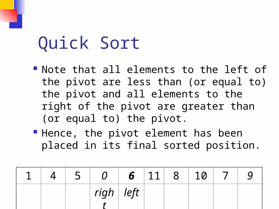
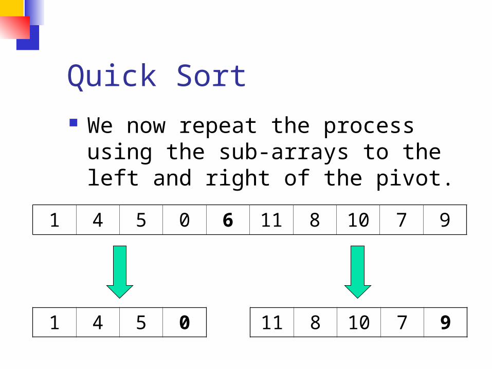
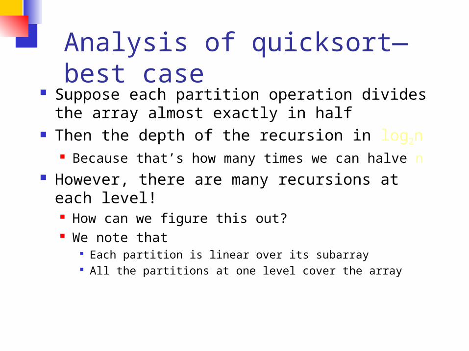
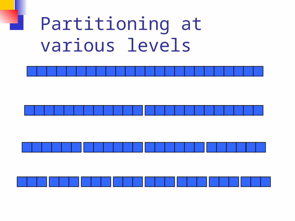
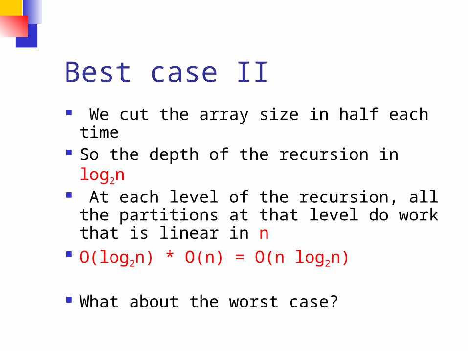
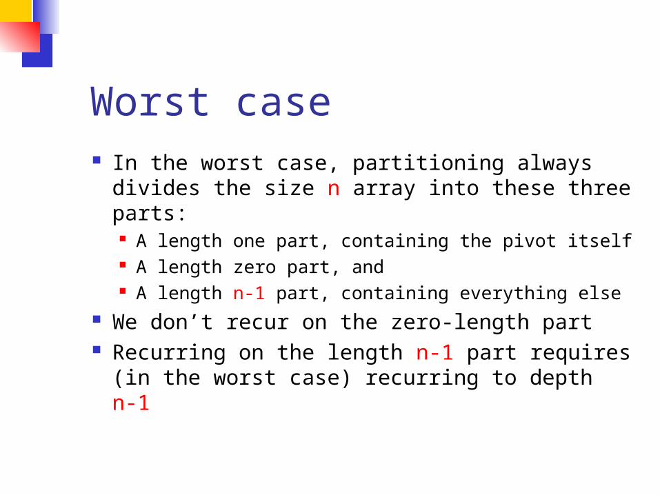
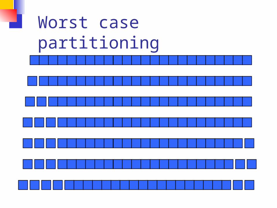
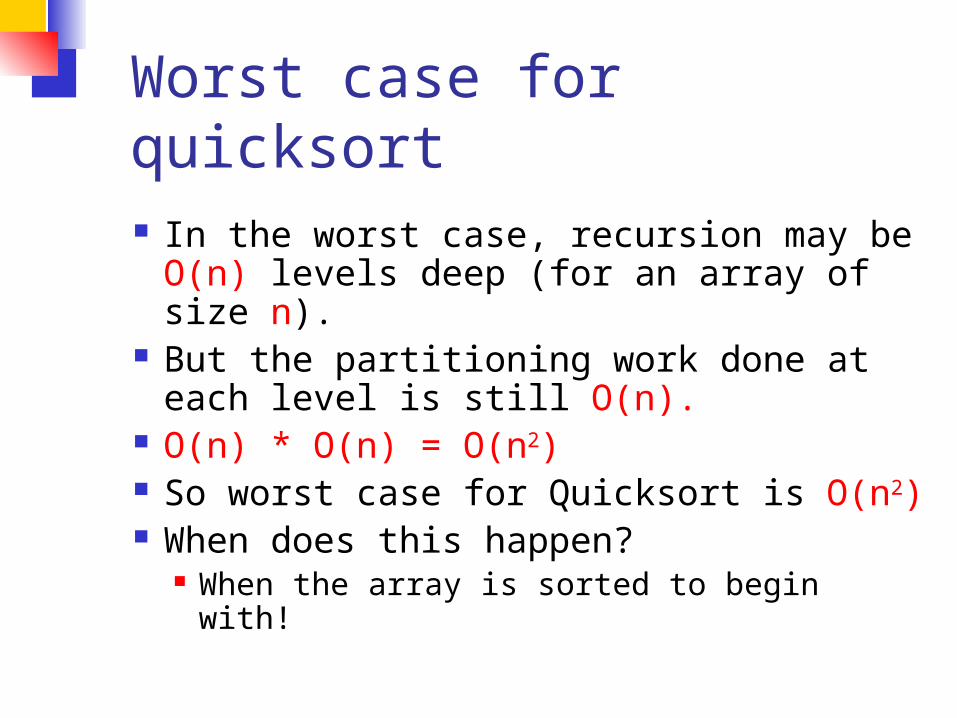
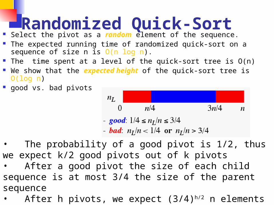
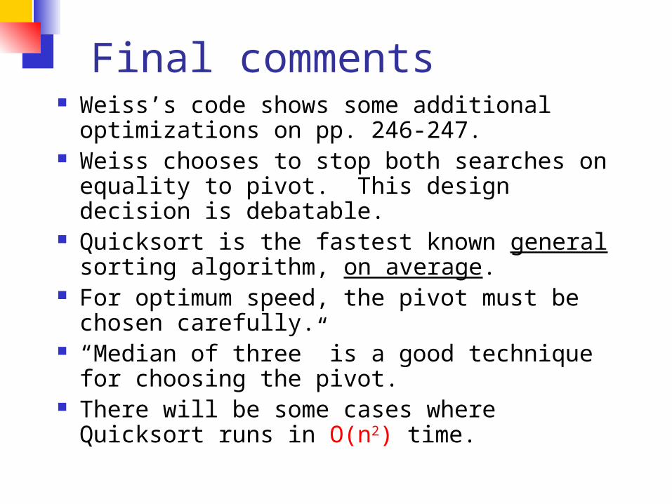
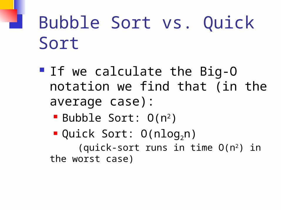
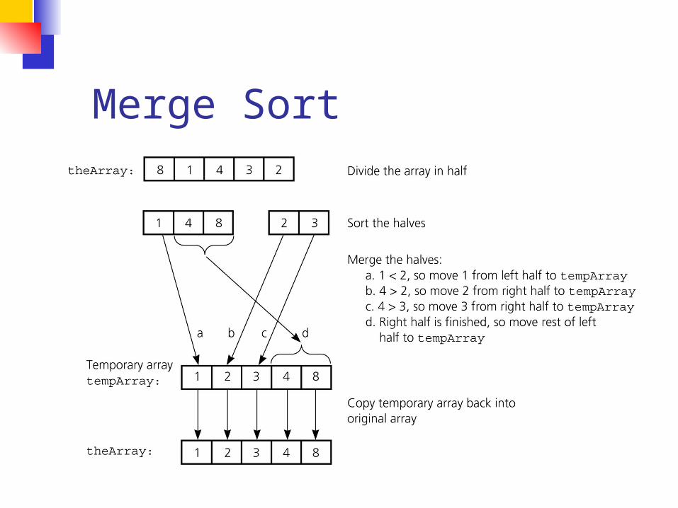
Merge Sort
Merge Sort Although the merge step produces
a sorted array we have overlooked a very important step
How did we sort the 2 halves before performing the merge step
We used merge sort
Merge Sort By continually calling the merge
sort algorithm we eventually get a subarray of size 1
Since an array with only 1 element is clearly sorted we can back out and merge 2 arrays of size 1
Merge Sort
Merge Sort The basic merging algorithm
consists of 2 input arrays (arrayA and arrayB) An ouput array (arrayC) 3 position holders (indexA indexB
indexC) which are initially set to the beginning of their respective arrays
Merge Sort The smaller of arrayA[indexA] and
arrayB[indexB] is copied into arrayC[indexC] and the appropriate position holders are advanced
When either input list is exhausted the remainder of the other list is copied into arrayC
Merge Sort
1 13 24 26index
A
indexC
arrayA
2 15 27 38index
B
arrayB
arrayC
We compare arrayA[indexA]with arrayB[indexB] Whichever value is smaller isplaced into arrayC[indexC]
1 lt 2 so we insert arrayA[indexA] intoarrayC[indexC]
Merge Sort
1 13 24 26indexA
1index
C
arrayA
2 15 27 38index
B
arrayB
arrayC
2 lt 13 so we insert arrayB[indexB] intoarrayC[indexC]
Merge Sort
1 13 24 26indexA
1 2index
C
arrayA
2 15 27 38indexB
arrayB
arrayC
13 lt 15 so we insert arrayA[indexA] intoarrayC[indexC]
Merge Sort
1 13 24 26indexA
1 2 13index
C
arrayA
2 15 27 38indexB
arrayB
arrayC
15 lt 24 so we insert arrayB[indexB] intoarrayC[indexC]
Merge Sort
1 13 24 26indexA
1 2 13 15indexC
arrayA
2 15 27 38indexB
arrayB
arrayC
24 lt 27 so we insert arrayA[indexA] intoarrayC[indexC]
Merge Sort
1 13 24
26
indexA
1 2 13 15 24indexC
arrayA
2 15 27 38indexB
arrayB
arrayC
26 lt 27 so we insert arrayA[indexA] intoarrayC[indexC]
Merge Sort
1 13 24
26
1 2 13 15 24 26indexC
arrayA
2 15 27 38indexB
arrayB
arrayC
Since we have exhaustedone of the arrays arrayAwe simply copy the remaining items from theother array arrayB intoarrayC
Merge Sort
1 13 24
26
1 2 13 15 24 26 27 38
arrayA
2 15 27 38arrayB
arrayC
Efficiency Summary
Sort Worst Case Average Case
Insertion O(n2) O(n2)
Shell O(n15) O(n125)
Selection O(n2) O(n2)
Bubble O(n2) O(n2)
Quick O(n2) O(nlog2n)
Heap O(nlog2n) O(nlog2n)
Merge O(nlog2n) O(nlog2n)
More Sorting
radix sort bucket sort in-place sorting how fast can we sort
Radix Sort
Unlike other sorting methods radix sort considers the structure of the keys
Assume keys are represented in a base M number system (M = radix) ie if M = 2 the keys are represented in binary
Sorting is done by comparing bits in the same position
Extension to keys that are alphanumeric strings
Radix Exchange Sort
Examine bits from left to right1 Sort array with respect to leftmost bit
2 Partition array
3Recursionrecursively sort top subarray ignoring leftmost bitrecursively sort bottom subarray ignoring leftmost bit
Time to sort n b-bit numbers O(b n)
Radix Exchange SortHow do we do the sort from the previous page Same idea as partition in Quicksort repeat
scan top-down to find key starting with 1scan bottom-up to find key starting with 0exchange keys
until scan indices cross
Radix Exchange Sort
Radix Exchange Sort vs Quicksort
Similaritiesboth partition arrayboth recursively sort sub-arrays
DifferencesMethod of partitioning
radix exchange divides array based on greater than or less than 2b-1
quicksort partitions based on greater than or less than some element of the array
Time complexityRadix exchange O (bn)Quicksort average case O (n log n)
Straight Radix Sort
Examines bits from right to left
for k = 0 to b-1 sort the array in a stable waylooking only at bit k
Note order of these bits after sort
Recall ldquosort in a stable
wayrdquo
In a stable sort the initial relative order of equal keys is unchangedFor example observe the first step of the sort from the previous page
Note that the relative order of those keys ending with 0 is unchanged and the same is true for elements ending in 1
The Algorithm is Correct (right)
We show that any two keys are in the correct relative order at the end of the algorithm
Given two keys let k be the leftmost bit-position where they differ
At step k the two keys are put in the correct relative orderBecause of stability the successive steps do not change the relative order of the two keys
For InstanceConsider a sort on an array with these two keys
Radix sorting can be applied to decimal numbers
Straight Radix SortTime Complexity
for k = 0 to b - 1 sort the array in a stable way looking only at bit k
Suppose we can perform the stable sort above in O(n) time The total time complexity would be
O(bn)As you might have guessed we can perform a stable sort based on the keysrsquo kth digit in O(n) time
The method you ask Why itrsquos Bucket Sort of course
Bucket Sort
BASICSn numbersEach number 1 2 3 mStableTime O (n + m)
For example m = 3 and our array is
(note that there are two ldquo2rdquos and two ldquo1rdquos)
First we create M ldquobucketsrdquo
Bucket SortEach element of the array is put in one of the m ldquobucketsrdquo
Bucket Sort
Now pull the elements from the buckets into the array
At last the sorted array (sorted in a stable way)
Comparison Sorting Elements are rearranged by comparing
values of keys Comparison of keys is interleaved with
rearrangements of the order of various pairs of keys as the algorithm progressively moves keys into final sorted order
Comparisons performed at given stage will depend on outcomes of previous comparisons and previous rearrangements of keys
Sorting an array of 3 elements a b and c produces 6 or 3 distinct orderings
Decision TreeConsider a decision tree that sorts n items The next slide shows a decision tree for 3 items a b c
Ovals represent comparisons If lt we traverse down a left branch
otherwise a right branch
Decision Tree on 3 Elements
a b c
bltc
bltc
altb
altc altc
a c b b a cc a b
c b a
b c a
true
true
true true
true
false
false
false
false
false
Levels in Decision Trees Number the levels starting at zero Level i can represent 2i arrangements Our decision tree can represent 8 = 23
arrangements If we have 4 items then 4 = 24 elements
but 4 levels gives at most 24 = 16 so we need 5 levels since 25 = 32 24
If we have k arrangements to represent then we need a decision tree with at least lg k levels
Size of Decision TreeWhen dealing with n elements we have n
possible arrangements and need a decision tree with at least lg n levels
)lg(2
lg2
2lg
2
)2lg()1lg(lg
)1lg()2lg()2lg()1lg(lg
))1)(2)(2)(1(lg()lg(
nn
nn
n
nn
nnn
nnn
nnnn
Lower Bound Resultn = n(n-1)(n-2)hellip21
from this we getlg(n) = lg(n) + lg(n-1) + lg(n-2) +hellip+
lg2 + lg1this means
lg(n) lt nlg(n)and the two results together show
O(lg(n)) = O(nlg(n))
No general sorting algorithm can run faster than O(n lg n)
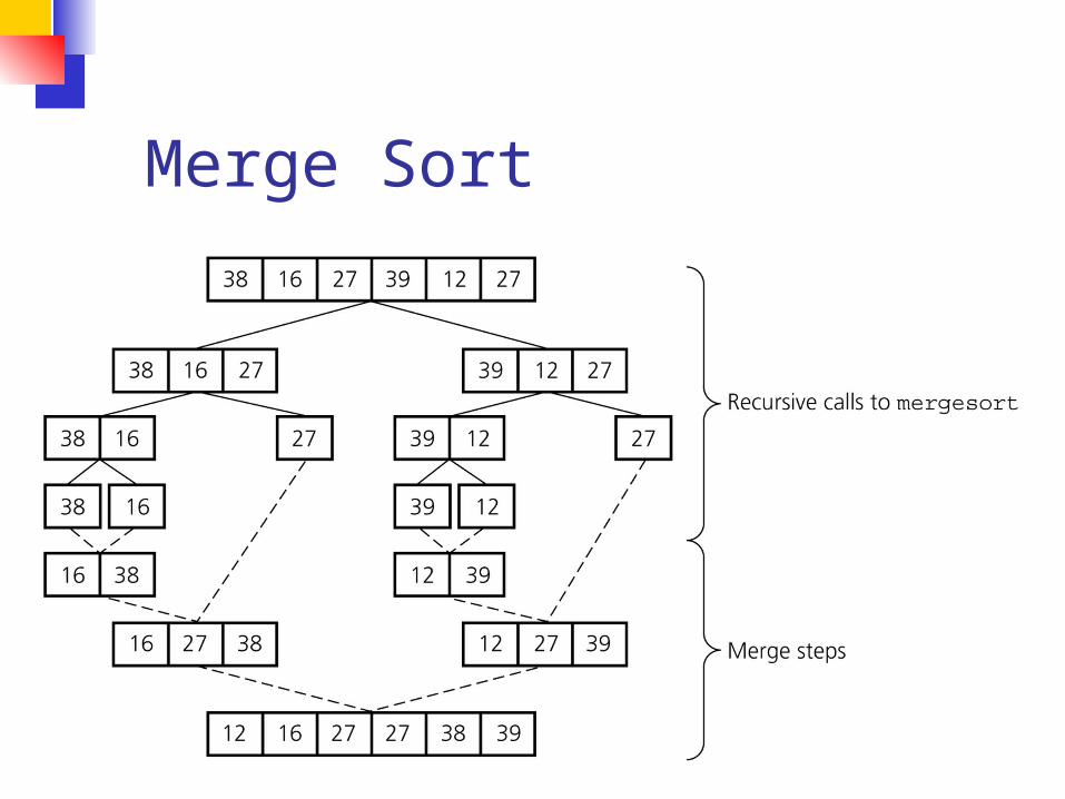
Merge Sort
Merge Sort The basic merging algorithm
consists of 2 input arrays (arrayA and arrayB) An ouput array (arrayC) 3 position holders (indexA indexB
indexC) which are initially set to the beginning of their respective arrays
Merge Sort The smaller of arrayA[indexA] and
arrayB[indexB] is copied into arrayC[indexC] and the appropriate position holders are advanced
When either input list is exhausted the remainder of the other list is copied into arrayC
Merge Sort
1 13 24 26index
A
indexC
arrayA
2 15 27 38index
B
arrayB
arrayC
We compare arrayA[indexA]with arrayB[indexB] Whichever value is smaller isplaced into arrayC[indexC]
1 lt 2 so we insert arrayA[indexA] intoarrayC[indexC]
Merge Sort
1 13 24 26indexA
1index
C
arrayA
2 15 27 38index
B
arrayB
arrayC
2 lt 13 so we insert arrayB[indexB] intoarrayC[indexC]
Merge Sort
1 13 24 26indexA
1 2index
C
arrayA
2 15 27 38indexB
arrayB
arrayC
13 lt 15 so we insert arrayA[indexA] intoarrayC[indexC]
Merge Sort
1 13 24 26indexA
1 2 13index
C
arrayA
2 15 27 38indexB
arrayB
arrayC
15 lt 24 so we insert arrayB[indexB] intoarrayC[indexC]
Merge Sort
1 13 24 26indexA
1 2 13 15indexC
arrayA
2 15 27 38indexB
arrayB
arrayC
24 lt 27 so we insert arrayA[indexA] intoarrayC[indexC]
Merge Sort
1 13 24
26
indexA
1 2 13 15 24indexC
arrayA
2 15 27 38indexB
arrayB
arrayC
26 lt 27 so we insert arrayA[indexA] intoarrayC[indexC]
Merge Sort
1 13 24
26
1 2 13 15 24 26indexC
arrayA
2 15 27 38indexB
arrayB
arrayC
Since we have exhaustedone of the arrays arrayAwe simply copy the remaining items from theother array arrayB intoarrayC
Merge Sort
1 13 24
26
1 2 13 15 24 26 27 38
arrayA
2 15 27 38arrayB
arrayC
Efficiency Summary
Sort Worst Case Average Case
Insertion O(n2) O(n2)
Shell O(n15) O(n125)
Selection O(n2) O(n2)
Bubble O(n2) O(n2)
Quick O(n2) O(nlog2n)
Heap O(nlog2n) O(nlog2n)
Merge O(nlog2n) O(nlog2n)
More Sorting
radix sort bucket sort in-place sorting how fast can we sort
Radix Sort
Unlike other sorting methods radix sort considers the structure of the keys
Assume keys are represented in a base M number system (M = radix) ie if M = 2 the keys are represented in binary
Sorting is done by comparing bits in the same position
Extension to keys that are alphanumeric strings
Radix Exchange Sort
Examine bits from left to right1 Sort array with respect to leftmost bit
2 Partition array
3Recursionrecursively sort top subarray ignoring leftmost bitrecursively sort bottom subarray ignoring leftmost bit
Time to sort n b-bit numbers O(b n)
Radix Exchange SortHow do we do the sort from the previous page Same idea as partition in Quicksort repeat
scan top-down to find key starting with 1scan bottom-up to find key starting with 0exchange keys
until scan indices cross
Radix Exchange Sort
Radix Exchange Sort vs Quicksort
Similaritiesboth partition arrayboth recursively sort sub-arrays
DifferencesMethod of partitioning
radix exchange divides array based on greater than or less than 2b-1
quicksort partitions based on greater than or less than some element of the array
Time complexityRadix exchange O (bn)Quicksort average case O (n log n)
Straight Radix Sort
Examines bits from right to left
for k = 0 to b-1 sort the array in a stable waylooking only at bit k
Note order of these bits after sort
Recall ldquosort in a stable
wayrdquo
In a stable sort the initial relative order of equal keys is unchangedFor example observe the first step of the sort from the previous page
Note that the relative order of those keys ending with 0 is unchanged and the same is true for elements ending in 1
The Algorithm is Correct (right)
We show that any two keys are in the correct relative order at the end of the algorithm
Given two keys let k be the leftmost bit-position where they differ
At step k the two keys are put in the correct relative orderBecause of stability the successive steps do not change the relative order of the two keys
For InstanceConsider a sort on an array with these two keys
Radix sorting can be applied to decimal numbers
Straight Radix SortTime Complexity
for k = 0 to b - 1 sort the array in a stable way looking only at bit k
Suppose we can perform the stable sort above in O(n) time The total time complexity would be
O(bn)As you might have guessed we can perform a stable sort based on the keysrsquo kth digit in O(n) time
The method you ask Why itrsquos Bucket Sort of course
Bucket Sort
BASICSn numbersEach number 1 2 3 mStableTime O (n + m)
For example m = 3 and our array is
(note that there are two ldquo2rdquos and two ldquo1rdquos)
First we create M ldquobucketsrdquo
Bucket SortEach element of the array is put in one of the m ldquobucketsrdquo
Bucket Sort
Now pull the elements from the buckets into the array
At last the sorted array (sorted in a stable way)
Comparison Sorting Elements are rearranged by comparing
values of keys Comparison of keys is interleaved with
rearrangements of the order of various pairs of keys as the algorithm progressively moves keys into final sorted order
Comparisons performed at given stage will depend on outcomes of previous comparisons and previous rearrangements of keys
Sorting an array of 3 elements a b and c produces 6 or 3 distinct orderings
Decision TreeConsider a decision tree that sorts n items The next slide shows a decision tree for 3 items a b c
Ovals represent comparisons If lt we traverse down a left branch
otherwise a right branch
Decision Tree on 3 Elements
a b c
bltc
bltc
altb
altc altc
a c b b a cc a b
c b a
b c a
true
true
true true
true
false
false
false
false
false
Levels in Decision Trees Number the levels starting at zero Level i can represent 2i arrangements Our decision tree can represent 8 = 23
arrangements If we have 4 items then 4 = 24 elements
but 4 levels gives at most 24 = 16 so we need 5 levels since 25 = 32 24
If we have k arrangements to represent then we need a decision tree with at least lg k levels
Size of Decision TreeWhen dealing with n elements we have n
possible arrangements and need a decision tree with at least lg n levels
)lg(2
lg2
2lg
2
)2lg()1lg(lg
)1lg()2lg()2lg()1lg(lg
))1)(2)(2)(1(lg()lg(
nn
nn
n
nn
nnn
nnn
nnnn
Lower Bound Resultn = n(n-1)(n-2)hellip21
from this we getlg(n) = lg(n) + lg(n-1) + lg(n-2) +hellip+
lg2 + lg1this means
lg(n) lt nlg(n)and the two results together show
O(lg(n)) = O(nlg(n))
No general sorting algorithm can run faster than O(n lg n)
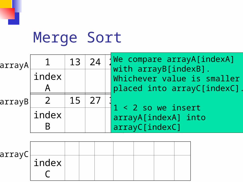
Merge Sort
1 13 24 26index
A
indexC
arrayA
2 15 27 38index
B
arrayB
arrayC
We compare arrayA[indexA]with arrayB[indexB] Whichever value is smaller isplaced into arrayC[indexC]
1 lt 2 so we insert arrayA[indexA] intoarrayC[indexC]
Merge Sort
1 13 24 26indexA
1index
C
arrayA
2 15 27 38index
B
arrayB
arrayC
2 lt 13 so we insert arrayB[indexB] intoarrayC[indexC]
Merge Sort
1 13 24 26indexA
1 2index
C
arrayA
2 15 27 38indexB
arrayB
arrayC
13 lt 15 so we insert arrayA[indexA] intoarrayC[indexC]
Merge Sort
1 13 24 26indexA
1 2 13index
C
arrayA
2 15 27 38indexB
arrayB
arrayC
15 lt 24 so we insert arrayB[indexB] intoarrayC[indexC]
Merge Sort
1 13 24 26indexA
1 2 13 15indexC
arrayA
2 15 27 38indexB
arrayB
arrayC
24 lt 27 so we insert arrayA[indexA] intoarrayC[indexC]
Merge Sort
1 13 24
26
indexA
1 2 13 15 24indexC
arrayA
2 15 27 38indexB
arrayB
arrayC
26 lt 27 so we insert arrayA[indexA] intoarrayC[indexC]
Merge Sort
1 13 24
26
1 2 13 15 24 26indexC
arrayA
2 15 27 38indexB
arrayB
arrayC
Since we have exhaustedone of the arrays arrayAwe simply copy the remaining items from theother array arrayB intoarrayC
Merge Sort
1 13 24
26
1 2 13 15 24 26 27 38
arrayA
2 15 27 38arrayB
arrayC
Efficiency Summary
Sort Worst Case Average Case
Insertion O(n2) O(n2)
Shell O(n15) O(n125)
Selection O(n2) O(n2)
Bubble O(n2) O(n2)
Quick O(n2) O(nlog2n)
Heap O(nlog2n) O(nlog2n)
Merge O(nlog2n) O(nlog2n)
More Sorting
radix sort bucket sort in-place sorting how fast can we sort
Radix Sort
Unlike other sorting methods radix sort considers the structure of the keys
Assume keys are represented in a base M number system (M = radix) ie if M = 2 the keys are represented in binary
Sorting is done by comparing bits in the same position
Extension to keys that are alphanumeric strings
Radix Exchange Sort
Examine bits from left to right1 Sort array with respect to leftmost bit
2 Partition array
3Recursionrecursively sort top subarray ignoring leftmost bitrecursively sort bottom subarray ignoring leftmost bit
Time to sort n b-bit numbers O(b n)
Radix Exchange SortHow do we do the sort from the previous page Same idea as partition in Quicksort repeat
scan top-down to find key starting with 1scan bottom-up to find key starting with 0exchange keys
until scan indices cross
Radix Exchange Sort
Radix Exchange Sort vs Quicksort
Similaritiesboth partition arrayboth recursively sort sub-arrays
DifferencesMethod of partitioning
radix exchange divides array based on greater than or less than 2b-1
quicksort partitions based on greater than or less than some element of the array
Time complexityRadix exchange O (bn)Quicksort average case O (n log n)
Straight Radix Sort
Examines bits from right to left
for k = 0 to b-1 sort the array in a stable waylooking only at bit k
Note order of these bits after sort
Recall ldquosort in a stable
wayrdquo
In a stable sort the initial relative order of equal keys is unchangedFor example observe the first step of the sort from the previous page
Note that the relative order of those keys ending with 0 is unchanged and the same is true for elements ending in 1
The Algorithm is Correct (right)
We show that any two keys are in the correct relative order at the end of the algorithm
Given two keys let k be the leftmost bit-position where they differ
At step k the two keys are put in the correct relative orderBecause of stability the successive steps do not change the relative order of the two keys
For InstanceConsider a sort on an array with these two keys
Radix sorting can be applied to decimal numbers
Straight Radix SortTime Complexity
for k = 0 to b - 1 sort the array in a stable way looking only at bit k
Suppose we can perform the stable sort above in O(n) time The total time complexity would be
O(bn)As you might have guessed we can perform a stable sort based on the keysrsquo kth digit in O(n) time
The method you ask Why itrsquos Bucket Sort of course
Bucket Sort
BASICSn numbersEach number 1 2 3 mStableTime O (n + m)
For example m = 3 and our array is
(note that there are two ldquo2rdquos and two ldquo1rdquos)
First we create M ldquobucketsrdquo
Bucket SortEach element of the array is put in one of the m ldquobucketsrdquo
Bucket Sort
Now pull the elements from the buckets into the array
At last the sorted array (sorted in a stable way)
Comparison Sorting Elements are rearranged by comparing
values of keys Comparison of keys is interleaved with
rearrangements of the order of various pairs of keys as the algorithm progressively moves keys into final sorted order
Comparisons performed at given stage will depend on outcomes of previous comparisons and previous rearrangements of keys
Sorting an array of 3 elements a b and c produces 6 or 3 distinct orderings
Decision TreeConsider a decision tree that sorts n items The next slide shows a decision tree for 3 items a b c
Ovals represent comparisons If lt we traverse down a left branch
otherwise a right branch
Decision Tree on 3 Elements
a b c
bltc
bltc
altb
altc altc
a c b b a cc a b
c b a
b c a
true
true
true true
true
false
false
false
false
false
Levels in Decision Trees Number the levels starting at zero Level i can represent 2i arrangements Our decision tree can represent 8 = 23
arrangements If we have 4 items then 4 = 24 elements
but 4 levels gives at most 24 = 16 so we need 5 levels since 25 = 32 24
If we have k arrangements to represent then we need a decision tree with at least lg k levels
Size of Decision TreeWhen dealing with n elements we have n
possible arrangements and need a decision tree with at least lg n levels
)lg(2
lg2
2lg
2
)2lg()1lg(lg
)1lg()2lg()2lg()1lg(lg
))1)(2)(2)(1(lg()lg(
nn
nn
n
nn
nnn
nnn
nnnn
Lower Bound Resultn = n(n-1)(n-2)hellip21
from this we getlg(n) = lg(n) + lg(n-1) + lg(n-2) +hellip+
lg2 + lg1this means
lg(n) lt nlg(n)and the two results together show
O(lg(n)) = O(nlg(n))
No general sorting algorithm can run faster than O(n lg n)
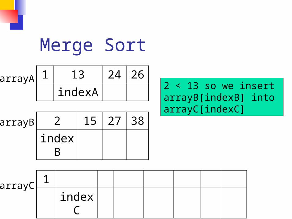
Merge Sort
1 13 24 26indexA
1index
C
arrayA
2 15 27 38index
B
arrayB
arrayC
2 lt 13 so we insert arrayB[indexB] intoarrayC[indexC]
Merge Sort
1 13 24 26indexA
1 2index
C
arrayA
2 15 27 38indexB
arrayB
arrayC
13 lt 15 so we insert arrayA[indexA] intoarrayC[indexC]
Merge Sort
1 13 24 26indexA
1 2 13index
C
arrayA
2 15 27 38indexB
arrayB
arrayC
15 lt 24 so we insert arrayB[indexB] intoarrayC[indexC]
Merge Sort
1 13 24 26indexA
1 2 13 15indexC
arrayA
2 15 27 38indexB
arrayB
arrayC
24 lt 27 so we insert arrayA[indexA] intoarrayC[indexC]
Merge Sort
1 13 24
26
indexA
1 2 13 15 24indexC
arrayA
2 15 27 38indexB
arrayB
arrayC
26 lt 27 so we insert arrayA[indexA] intoarrayC[indexC]
Merge Sort
1 13 24
26
1 2 13 15 24 26indexC
arrayA
2 15 27 38indexB
arrayB
arrayC
Since we have exhaustedone of the arrays arrayAwe simply copy the remaining items from theother array arrayB intoarrayC
Merge Sort
1 13 24
26
1 2 13 15 24 26 27 38
arrayA
2 15 27 38arrayB
arrayC
Efficiency Summary
Sort Worst Case Average Case
Insertion O(n2) O(n2)
Shell O(n15) O(n125)
Selection O(n2) O(n2)
Bubble O(n2) O(n2)
Quick O(n2) O(nlog2n)
Heap O(nlog2n) O(nlog2n)
Merge O(nlog2n) O(nlog2n)
More Sorting
radix sort bucket sort in-place sorting how fast can we sort
Radix Sort
Unlike other sorting methods radix sort considers the structure of the keys
Assume keys are represented in a base M number system (M = radix) ie if M = 2 the keys are represented in binary
Sorting is done by comparing bits in the same position
Extension to keys that are alphanumeric strings
Radix Exchange Sort
Examine bits from left to right1 Sort array with respect to leftmost bit
2 Partition array
3Recursionrecursively sort top subarray ignoring leftmost bitrecursively sort bottom subarray ignoring leftmost bit
Time to sort n b-bit numbers O(b n)
Radix Exchange SortHow do we do the sort from the previous page Same idea as partition in Quicksort repeat
scan top-down to find key starting with 1scan bottom-up to find key starting with 0exchange keys
until scan indices cross
Radix Exchange Sort
Radix Exchange Sort vs Quicksort
Similaritiesboth partition arrayboth recursively sort sub-arrays
DifferencesMethod of partitioning
radix exchange divides array based on greater than or less than 2b-1
quicksort partitions based on greater than or less than some element of the array
Time complexityRadix exchange O (bn)Quicksort average case O (n log n)
Straight Radix Sort
Examines bits from right to left
for k = 0 to b-1 sort the array in a stable waylooking only at bit k
Note order of these bits after sort
Recall ldquosort in a stable
wayrdquo
In a stable sort the initial relative order of equal keys is unchangedFor example observe the first step of the sort from the previous page
Note that the relative order of those keys ending with 0 is unchanged and the same is true for elements ending in 1
The Algorithm is Correct (right)
We show that any two keys are in the correct relative order at the end of the algorithm
Given two keys let k be the leftmost bit-position where they differ
At step k the two keys are put in the correct relative orderBecause of stability the successive steps do not change the relative order of the two keys
For InstanceConsider a sort on an array with these two keys
Radix sorting can be applied to decimal numbers
Straight Radix SortTime Complexity
for k = 0 to b - 1 sort the array in a stable way looking only at bit k
Suppose we can perform the stable sort above in O(n) time The total time complexity would be
O(bn)As you might have guessed we can perform a stable sort based on the keysrsquo kth digit in O(n) time
The method you ask Why itrsquos Bucket Sort of course
Bucket Sort
BASICSn numbersEach number 1 2 3 mStableTime O (n + m)
For example m = 3 and our array is
(note that there are two ldquo2rdquos and two ldquo1rdquos)
First we create M ldquobucketsrdquo
Bucket SortEach element of the array is put in one of the m ldquobucketsrdquo
Bucket Sort
Now pull the elements from the buckets into the array
At last the sorted array (sorted in a stable way)
Comparison Sorting Elements are rearranged by comparing
values of keys Comparison of keys is interleaved with
rearrangements of the order of various pairs of keys as the algorithm progressively moves keys into final sorted order
Comparisons performed at given stage will depend on outcomes of previous comparisons and previous rearrangements of keys
Sorting an array of 3 elements a b and c produces 6 or 3 distinct orderings
Decision TreeConsider a decision tree that sorts n items The next slide shows a decision tree for 3 items a b c
Ovals represent comparisons If lt we traverse down a left branch
otherwise a right branch
Decision Tree on 3 Elements
a b c
bltc
bltc
altb
altc altc
a c b b a cc a b
c b a
b c a
true
true
true true
true
false
false
false
false
false
Levels in Decision Trees Number the levels starting at zero Level i can represent 2i arrangements Our decision tree can represent 8 = 23
arrangements If we have 4 items then 4 = 24 elements
but 4 levels gives at most 24 = 16 so we need 5 levels since 25 = 32 24
If we have k arrangements to represent then we need a decision tree with at least lg k levels
Size of Decision TreeWhen dealing with n elements we have n
possible arrangements and need a decision tree with at least lg n levels
)lg(2
lg2
2lg
2
)2lg()1lg(lg
)1lg()2lg()2lg()1lg(lg
))1)(2)(2)(1(lg()lg(
nn
nn
n
nn
nnn
nnn
nnnn
Lower Bound Resultn = n(n-1)(n-2)hellip21
from this we getlg(n) = lg(n) + lg(n-1) + lg(n-2) +hellip+
lg2 + lg1this means
lg(n) lt nlg(n)and the two results together show
O(lg(n)) = O(nlg(n))
No general sorting algorithm can run faster than O(n lg n)
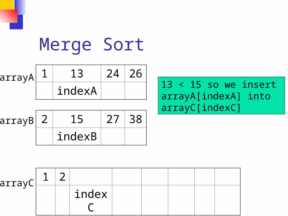
Merge Sort
1 13 24 26indexA
1 2index
C
arrayA
2 15 27 38indexB
arrayB
arrayC
13 lt 15 so we insert arrayA[indexA] intoarrayC[indexC]
Merge Sort
1 13 24 26indexA
1 2 13index
C
arrayA
2 15 27 38indexB
arrayB
arrayC
15 lt 24 so we insert arrayB[indexB] intoarrayC[indexC]
Merge Sort
1 13 24 26indexA
1 2 13 15indexC
arrayA
2 15 27 38indexB
arrayB
arrayC
24 lt 27 so we insert arrayA[indexA] intoarrayC[indexC]
Merge Sort
1 13 24
26
indexA
1 2 13 15 24indexC
arrayA
2 15 27 38indexB
arrayB
arrayC
26 lt 27 so we insert arrayA[indexA] intoarrayC[indexC]
Merge Sort
1 13 24
26
1 2 13 15 24 26indexC
arrayA
2 15 27 38indexB
arrayB
arrayC
Since we have exhaustedone of the arrays arrayAwe simply copy the remaining items from theother array arrayB intoarrayC
Merge Sort
1 13 24
26
1 2 13 15 24 26 27 38
arrayA
2 15 27 38arrayB
arrayC
Efficiency Summary
Sort Worst Case Average Case
Insertion O(n2) O(n2)
Shell O(n15) O(n125)
Selection O(n2) O(n2)
Bubble O(n2) O(n2)
Quick O(n2) O(nlog2n)
Heap O(nlog2n) O(nlog2n)
Merge O(nlog2n) O(nlog2n)
More Sorting
radix sort bucket sort in-place sorting how fast can we sort
Radix Sort
Unlike other sorting methods radix sort considers the structure of the keys
Assume keys are represented in a base M number system (M = radix) ie if M = 2 the keys are represented in binary
Sorting is done by comparing bits in the same position
Extension to keys that are alphanumeric strings
Radix Exchange Sort
Examine bits from left to right1 Sort array with respect to leftmost bit
2 Partition array
3Recursionrecursively sort top subarray ignoring leftmost bitrecursively sort bottom subarray ignoring leftmost bit
Time to sort n b-bit numbers O(b n)
Radix Exchange SortHow do we do the sort from the previous page Same idea as partition in Quicksort repeat
scan top-down to find key starting with 1scan bottom-up to find key starting with 0exchange keys
until scan indices cross
Radix Exchange Sort
Radix Exchange Sort vs Quicksort
Similaritiesboth partition arrayboth recursively sort sub-arrays
DifferencesMethod of partitioning
radix exchange divides array based on greater than or less than 2b-1
quicksort partitions based on greater than or less than some element of the array
Time complexityRadix exchange O (bn)Quicksort average case O (n log n)
Straight Radix Sort
Examines bits from right to left
for k = 0 to b-1 sort the array in a stable waylooking only at bit k
Note order of these bits after sort
Recall ldquosort in a stable
wayrdquo
In a stable sort the initial relative order of equal keys is unchangedFor example observe the first step of the sort from the previous page
Note that the relative order of those keys ending with 0 is unchanged and the same is true for elements ending in 1
The Algorithm is Correct (right)
We show that any two keys are in the correct relative order at the end of the algorithm
Given two keys let k be the leftmost bit-position where they differ
At step k the two keys are put in the correct relative orderBecause of stability the successive steps do not change the relative order of the two keys
For InstanceConsider a sort on an array with these two keys
Radix sorting can be applied to decimal numbers
Straight Radix SortTime Complexity
for k = 0 to b - 1 sort the array in a stable way looking only at bit k
Suppose we can perform the stable sort above in O(n) time The total time complexity would be
O(bn)As you might have guessed we can perform a stable sort based on the keysrsquo kth digit in O(n) time
The method you ask Why itrsquos Bucket Sort of course
Bucket Sort
BASICSn numbersEach number 1 2 3 mStableTime O (n + m)
For example m = 3 and our array is
(note that there are two ldquo2rdquos and two ldquo1rdquos)
First we create M ldquobucketsrdquo
Bucket SortEach element of the array is put in one of the m ldquobucketsrdquo
Bucket Sort
Now pull the elements from the buckets into the array
At last the sorted array (sorted in a stable way)
Comparison Sorting Elements are rearranged by comparing
values of keys Comparison of keys is interleaved with
rearrangements of the order of various pairs of keys as the algorithm progressively moves keys into final sorted order
Comparisons performed at given stage will depend on outcomes of previous comparisons and previous rearrangements of keys
Sorting an array of 3 elements a b and c produces 6 or 3 distinct orderings
Decision TreeConsider a decision tree that sorts n items The next slide shows a decision tree for 3 items a b c
Ovals represent comparisons If lt we traverse down a left branch
otherwise a right branch
Decision Tree on 3 Elements
a b c
bltc
bltc
altb
altc altc
a c b b a cc a b
c b a
b c a
true
true
true true
true
false
false
false
false
false
Levels in Decision Trees Number the levels starting at zero Level i can represent 2i arrangements Our decision tree can represent 8 = 23
arrangements If we have 4 items then 4 = 24 elements
but 4 levels gives at most 24 = 16 so we need 5 levels since 25 = 32 24
If we have k arrangements to represent then we need a decision tree with at least lg k levels
Size of Decision TreeWhen dealing with n elements we have n
possible arrangements and need a decision tree with at least lg n levels
)lg(2
lg2
2lg
2
)2lg()1lg(lg
)1lg()2lg()2lg()1lg(lg
))1)(2)(2)(1(lg()lg(
nn
nn
n
nn
nnn
nnn
nnnn
Lower Bound Resultn = n(n-1)(n-2)hellip21
from this we getlg(n) = lg(n) + lg(n-1) + lg(n-2) +hellip+
lg2 + lg1this means
lg(n) lt nlg(n)and the two results together show
O(lg(n)) = O(nlg(n))
No general sorting algorithm can run faster than O(n lg n)
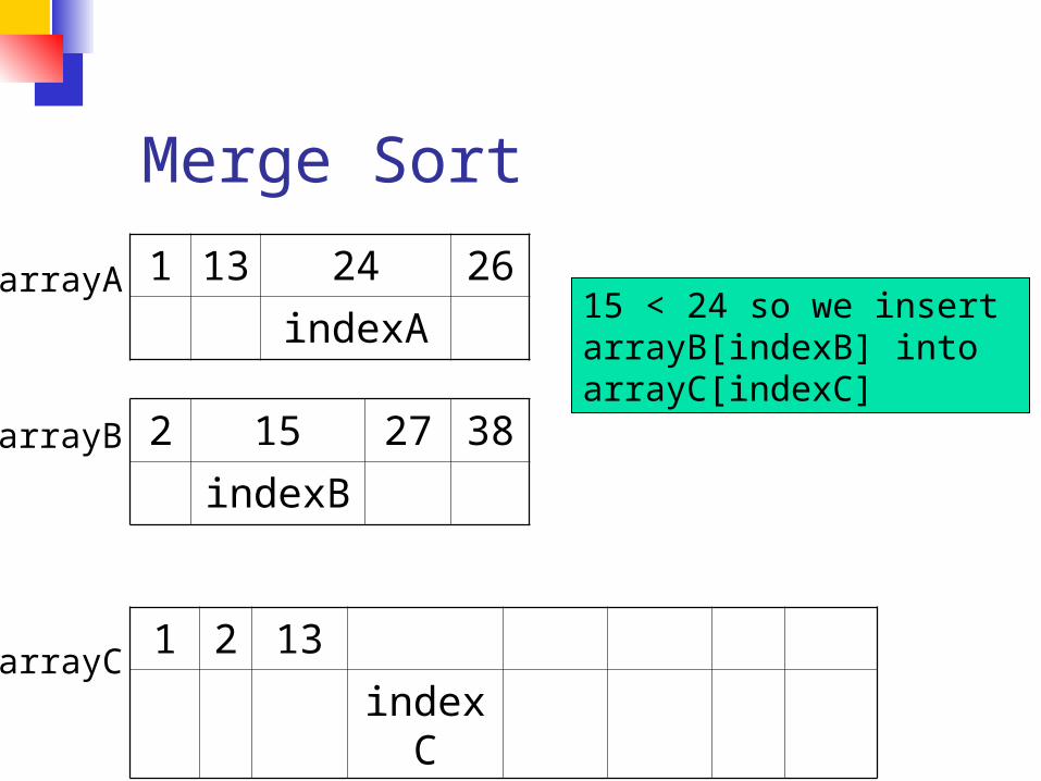
Merge Sort
1 13 24 26indexA
1 2 13index
C
arrayA
2 15 27 38indexB
arrayB
arrayC
15 lt 24 so we insert arrayB[indexB] intoarrayC[indexC]
Merge Sort
1 13 24 26indexA
1 2 13 15indexC
arrayA
2 15 27 38indexB
arrayB
arrayC
24 lt 27 so we insert arrayA[indexA] intoarrayC[indexC]
Merge Sort
1 13 24
26
indexA
1 2 13 15 24indexC
arrayA
2 15 27 38indexB
arrayB
arrayC
26 lt 27 so we insert arrayA[indexA] intoarrayC[indexC]
Merge Sort
1 13 24
26
1 2 13 15 24 26indexC
arrayA
2 15 27 38indexB
arrayB
arrayC
Since we have exhaustedone of the arrays arrayAwe simply copy the remaining items from theother array arrayB intoarrayC
Merge Sort
1 13 24
26
1 2 13 15 24 26 27 38
arrayA
2 15 27 38arrayB
arrayC
Efficiency Summary
Sort Worst Case Average Case
Insertion O(n2) O(n2)
Shell O(n15) O(n125)
Selection O(n2) O(n2)
Bubble O(n2) O(n2)
Quick O(n2) O(nlog2n)
Heap O(nlog2n) O(nlog2n)
Merge O(nlog2n) O(nlog2n)
More Sorting
radix sort bucket sort in-place sorting how fast can we sort
Radix Sort
Unlike other sorting methods radix sort considers the structure of the keys
Assume keys are represented in a base M number system (M = radix) ie if M = 2 the keys are represented in binary
Sorting is done by comparing bits in the same position
Extension to keys that are alphanumeric strings
Radix Exchange Sort
Examine bits from left to right1 Sort array with respect to leftmost bit
2 Partition array
3Recursionrecursively sort top subarray ignoring leftmost bitrecursively sort bottom subarray ignoring leftmost bit
Time to sort n b-bit numbers O(b n)
Radix Exchange SortHow do we do the sort from the previous page Same idea as partition in Quicksort repeat
scan top-down to find key starting with 1scan bottom-up to find key starting with 0exchange keys
until scan indices cross
Radix Exchange Sort
Radix Exchange Sort vs Quicksort
Similaritiesboth partition arrayboth recursively sort sub-arrays
DifferencesMethod of partitioning
radix exchange divides array based on greater than or less than 2b-1
quicksort partitions based on greater than or less than some element of the array
Time complexityRadix exchange O (bn)Quicksort average case O (n log n)
Straight Radix Sort
Examines bits from right to left
for k = 0 to b-1 sort the array in a stable waylooking only at bit k
Note order of these bits after sort
Recall ldquosort in a stable
wayrdquo
In a stable sort the initial relative order of equal keys is unchangedFor example observe the first step of the sort from the previous page
Note that the relative order of those keys ending with 0 is unchanged and the same is true for elements ending in 1
The Algorithm is Correct (right)
We show that any two keys are in the correct relative order at the end of the algorithm
Given two keys let k be the leftmost bit-position where they differ
At step k the two keys are put in the correct relative orderBecause of stability the successive steps do not change the relative order of the two keys
For InstanceConsider a sort on an array with these two keys
Radix sorting can be applied to decimal numbers
Straight Radix SortTime Complexity
for k = 0 to b - 1 sort the array in a stable way looking only at bit k
Suppose we can perform the stable sort above in O(n) time The total time complexity would be
O(bn)As you might have guessed we can perform a stable sort based on the keysrsquo kth digit in O(n) time
The method you ask Why itrsquos Bucket Sort of course
Bucket Sort
BASICSn numbersEach number 1 2 3 mStableTime O (n + m)
For example m = 3 and our array is
(note that there are two ldquo2rdquos and two ldquo1rdquos)
First we create M ldquobucketsrdquo
Bucket SortEach element of the array is put in one of the m ldquobucketsrdquo
Bucket Sort
Now pull the elements from the buckets into the array
At last the sorted array (sorted in a stable way)
Comparison Sorting Elements are rearranged by comparing
values of keys Comparison of keys is interleaved with
rearrangements of the order of various pairs of keys as the algorithm progressively moves keys into final sorted order
Comparisons performed at given stage will depend on outcomes of previous comparisons and previous rearrangements of keys
Sorting an array of 3 elements a b and c produces 6 or 3 distinct orderings
Decision TreeConsider a decision tree that sorts n items The next slide shows a decision tree for 3 items a b c
Ovals represent comparisons If lt we traverse down a left branch
otherwise a right branch
Decision Tree on 3 Elements
a b c
bltc
bltc
altb
altc altc
a c b b a cc a b
c b a
b c a
true
true
true true
true
false
false
false
false
false
Levels in Decision Trees Number the levels starting at zero Level i can represent 2i arrangements Our decision tree can represent 8 = 23
arrangements If we have 4 items then 4 = 24 elements
but 4 levels gives at most 24 = 16 so we need 5 levels since 25 = 32 24
If we have k arrangements to represent then we need a decision tree with at least lg k levels
Size of Decision TreeWhen dealing with n elements we have n
possible arrangements and need a decision tree with at least lg n levels
)lg(2
lg2
2lg
2
)2lg()1lg(lg
)1lg()2lg()2lg()1lg(lg
))1)(2)(2)(1(lg()lg(
nn
nn
n
nn
nnn
nnn
nnnn
Lower Bound Resultn = n(n-1)(n-2)hellip21
from this we getlg(n) = lg(n) + lg(n-1) + lg(n-2) +hellip+
lg2 + lg1this means
lg(n) lt nlg(n)and the two results together show
O(lg(n)) = O(nlg(n))
No general sorting algorithm can run faster than O(n lg n)
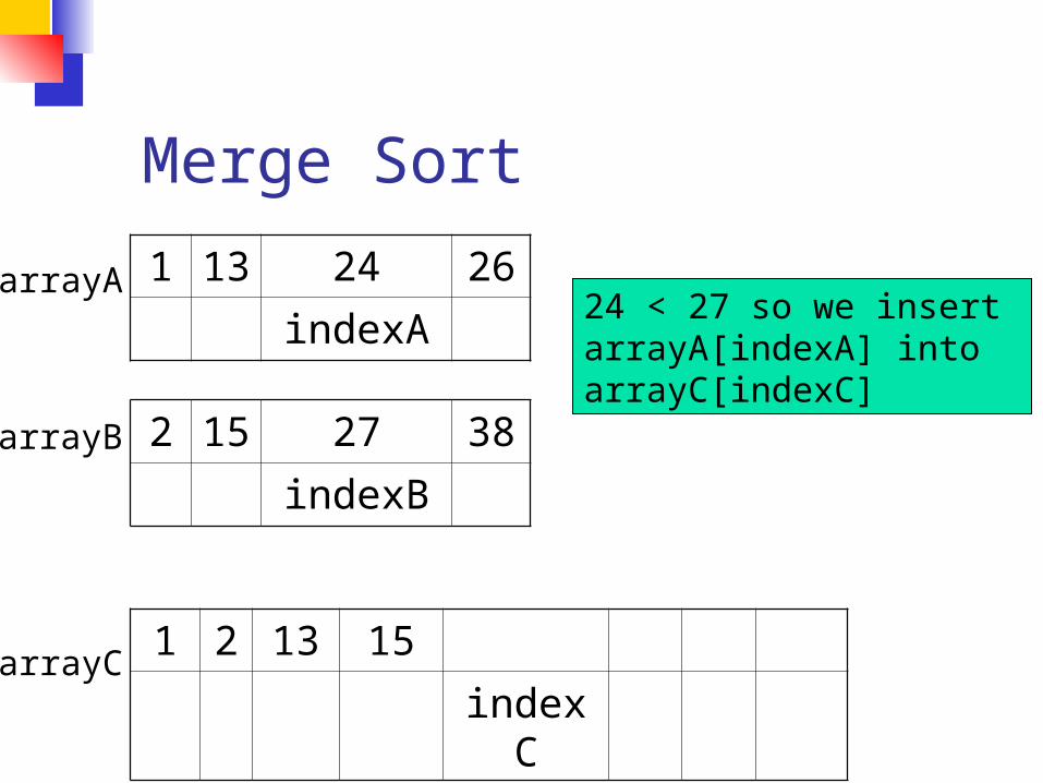
Merge Sort
1 13 24 26indexA
1 2 13 15indexC
arrayA
2 15 27 38indexB
arrayB
arrayC
24 lt 27 so we insert arrayA[indexA] intoarrayC[indexC]
Merge Sort
1 13 24
26
indexA
1 2 13 15 24indexC
arrayA
2 15 27 38indexB
arrayB
arrayC
26 lt 27 so we insert arrayA[indexA] intoarrayC[indexC]
Merge Sort
1 13 24
26
1 2 13 15 24 26indexC
arrayA
2 15 27 38indexB
arrayB
arrayC
Since we have exhaustedone of the arrays arrayAwe simply copy the remaining items from theother array arrayB intoarrayC
Merge Sort
1 13 24
26
1 2 13 15 24 26 27 38
arrayA
2 15 27 38arrayB
arrayC
Efficiency Summary
Sort Worst Case Average Case
Insertion O(n2) O(n2)
Shell O(n15) O(n125)
Selection O(n2) O(n2)
Bubble O(n2) O(n2)
Quick O(n2) O(nlog2n)
Heap O(nlog2n) O(nlog2n)
Merge O(nlog2n) O(nlog2n)
More Sorting
radix sort bucket sort in-place sorting how fast can we sort
Radix Sort
Unlike other sorting methods radix sort considers the structure of the keys
Assume keys are represented in a base M number system (M = radix) ie if M = 2 the keys are represented in binary
Sorting is done by comparing bits in the same position
Extension to keys that are alphanumeric strings
Radix Exchange Sort
Examine bits from left to right1 Sort array with respect to leftmost bit
2 Partition array
3Recursionrecursively sort top subarray ignoring leftmost bitrecursively sort bottom subarray ignoring leftmost bit
Time to sort n b-bit numbers O(b n)
Radix Exchange SortHow do we do the sort from the previous page Same idea as partition in Quicksort repeat
scan top-down to find key starting with 1scan bottom-up to find key starting with 0exchange keys
until scan indices cross
Radix Exchange Sort
Radix Exchange Sort vs Quicksort
Similaritiesboth partition arrayboth recursively sort sub-arrays
DifferencesMethod of partitioning
radix exchange divides array based on greater than or less than 2b-1
quicksort partitions based on greater than or less than some element of the array
Time complexityRadix exchange O (bn)Quicksort average case O (n log n)
Straight Radix Sort
Examines bits from right to left
for k = 0 to b-1 sort the array in a stable waylooking only at bit k
Note order of these bits after sort
Recall ldquosort in a stable
wayrdquo
In a stable sort the initial relative order of equal keys is unchangedFor example observe the first step of the sort from the previous page
Note that the relative order of those keys ending with 0 is unchanged and the same is true for elements ending in 1
The Algorithm is Correct (right)
We show that any two keys are in the correct relative order at the end of the algorithm
Given two keys let k be the leftmost bit-position where they differ
At step k the two keys are put in the correct relative orderBecause of stability the successive steps do not change the relative order of the two keys
For InstanceConsider a sort on an array with these two keys
Radix sorting can be applied to decimal numbers
Straight Radix SortTime Complexity
for k = 0 to b - 1 sort the array in a stable way looking only at bit k
Suppose we can perform the stable sort above in O(n) time The total time complexity would be
O(bn)As you might have guessed we can perform a stable sort based on the keysrsquo kth digit in O(n) time
The method you ask Why itrsquos Bucket Sort of course
Bucket Sort
BASICSn numbersEach number 1 2 3 mStableTime O (n + m)
For example m = 3 and our array is
(note that there are two ldquo2rdquos and two ldquo1rdquos)
First we create M ldquobucketsrdquo
Bucket SortEach element of the array is put in one of the m ldquobucketsrdquo
Bucket Sort
Now pull the elements from the buckets into the array
At last the sorted array (sorted in a stable way)
Comparison Sorting Elements are rearranged by comparing
values of keys Comparison of keys is interleaved with
rearrangements of the order of various pairs of keys as the algorithm progressively moves keys into final sorted order
Comparisons performed at given stage will depend on outcomes of previous comparisons and previous rearrangements of keys
Sorting an array of 3 elements a b and c produces 6 or 3 distinct orderings
Decision TreeConsider a decision tree that sorts n items The next slide shows a decision tree for 3 items a b c
Ovals represent comparisons If lt we traverse down a left branch
otherwise a right branch
Decision Tree on 3 Elements
a b c
bltc
bltc
altb
altc altc
a c b b a cc a b
c b a
b c a
true
true
true true
true
false
false
false
false
false
Levels in Decision Trees Number the levels starting at zero Level i can represent 2i arrangements Our decision tree can represent 8 = 23
arrangements If we have 4 items then 4 = 24 elements
but 4 levels gives at most 24 = 16 so we need 5 levels since 25 = 32 24
If we have k arrangements to represent then we need a decision tree with at least lg k levels
Size of Decision TreeWhen dealing with n elements we have n
possible arrangements and need a decision tree with at least lg n levels
)lg(2
lg2
2lg
2
)2lg()1lg(lg
)1lg()2lg()2lg()1lg(lg
))1)(2)(2)(1(lg()lg(
nn
nn
n
nn
nnn
nnn
nnnn
Lower Bound Resultn = n(n-1)(n-2)hellip21
from this we getlg(n) = lg(n) + lg(n-1) + lg(n-2) +hellip+
lg2 + lg1this means
lg(n) lt nlg(n)and the two results together show
O(lg(n)) = O(nlg(n))
No general sorting algorithm can run faster than O(n lg n)
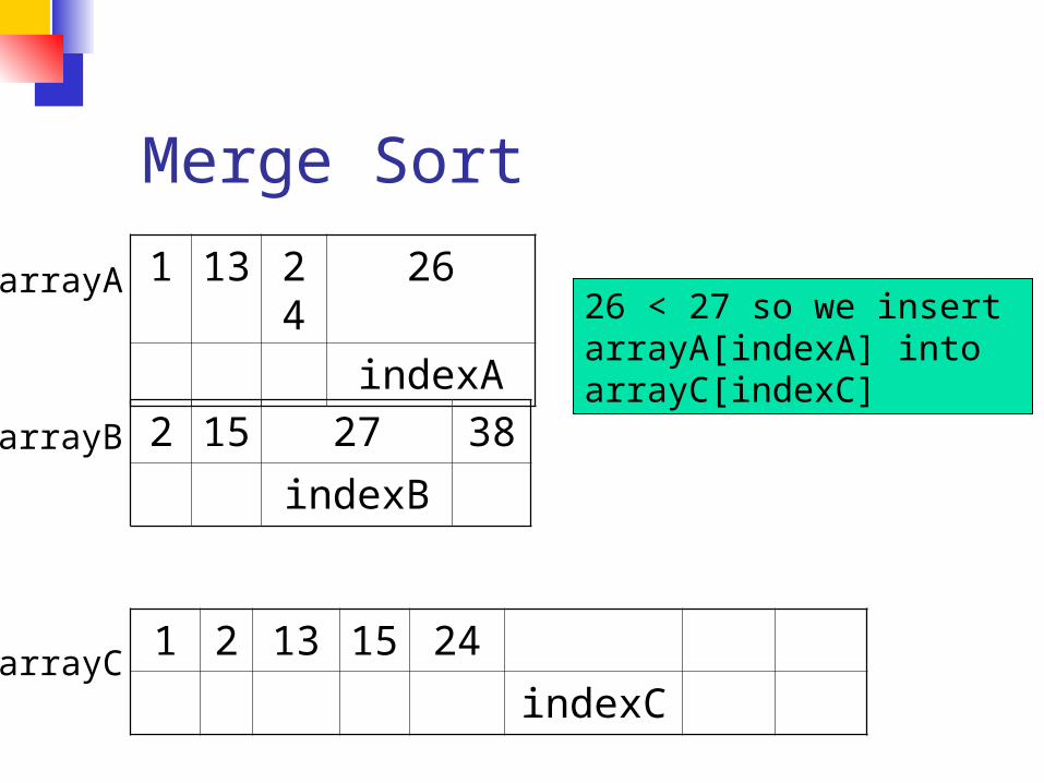
Merge Sort
1 13 24
26
indexA
1 2 13 15 24indexC
arrayA
2 15 27 38indexB
arrayB
arrayC
26 lt 27 so we insert arrayA[indexA] intoarrayC[indexC]
Merge Sort
1 13 24
26
1 2 13 15 24 26indexC
arrayA
2 15 27 38indexB
arrayB
arrayC
Since we have exhaustedone of the arrays arrayAwe simply copy the remaining items from theother array arrayB intoarrayC
Merge Sort
1 13 24
26
1 2 13 15 24 26 27 38
arrayA
2 15 27 38arrayB
arrayC
Efficiency Summary
Sort Worst Case Average Case
Insertion O(n2) O(n2)
Shell O(n15) O(n125)
Selection O(n2) O(n2)
Bubble O(n2) O(n2)
Quick O(n2) O(nlog2n)
Heap O(nlog2n) O(nlog2n)
Merge O(nlog2n) O(nlog2n)
More Sorting
radix sort bucket sort in-place sorting how fast can we sort
Radix Sort
Unlike other sorting methods radix sort considers the structure of the keys
Assume keys are represented in a base M number system (M = radix) ie if M = 2 the keys are represented in binary
Sorting is done by comparing bits in the same position
Extension to keys that are alphanumeric strings
Radix Exchange Sort
Examine bits from left to right1 Sort array with respect to leftmost bit
2 Partition array
3Recursionrecursively sort top subarray ignoring leftmost bitrecursively sort bottom subarray ignoring leftmost bit
Time to sort n b-bit numbers O(b n)
Radix Exchange SortHow do we do the sort from the previous page Same idea as partition in Quicksort repeat
scan top-down to find key starting with 1scan bottom-up to find key starting with 0exchange keys
until scan indices cross
Radix Exchange Sort
Radix Exchange Sort vs Quicksort
Similaritiesboth partition arrayboth recursively sort sub-arrays
DifferencesMethod of partitioning
radix exchange divides array based on greater than or less than 2b-1
quicksort partitions based on greater than or less than some element of the array
Time complexityRadix exchange O (bn)Quicksort average case O (n log n)
Straight Radix Sort
Examines bits from right to left
for k = 0 to b-1 sort the array in a stable waylooking only at bit k
Note order of these bits after sort
Recall ldquosort in a stable
wayrdquo
In a stable sort the initial relative order of equal keys is unchangedFor example observe the first step of the sort from the previous page
Note that the relative order of those keys ending with 0 is unchanged and the same is true for elements ending in 1
The Algorithm is Correct (right)
We show that any two keys are in the correct relative order at the end of the algorithm
Given two keys let k be the leftmost bit-position where they differ
At step k the two keys are put in the correct relative orderBecause of stability the successive steps do not change the relative order of the two keys
For InstanceConsider a sort on an array with these two keys
Radix sorting can be applied to decimal numbers
Straight Radix SortTime Complexity
for k = 0 to b - 1 sort the array in a stable way looking only at bit k
Suppose we can perform the stable sort above in O(n) time The total time complexity would be
O(bn)As you might have guessed we can perform a stable sort based on the keysrsquo kth digit in O(n) time
The method you ask Why itrsquos Bucket Sort of course
Bucket Sort
BASICSn numbersEach number 1 2 3 mStableTime O (n + m)
For example m = 3 and our array is
(note that there are two ldquo2rdquos and two ldquo1rdquos)
First we create M ldquobucketsrdquo
Bucket SortEach element of the array is put in one of the m ldquobucketsrdquo
Bucket Sort
Now pull the elements from the buckets into the array
At last the sorted array (sorted in a stable way)
Comparison Sorting Elements are rearranged by comparing
values of keys Comparison of keys is interleaved with
rearrangements of the order of various pairs of keys as the algorithm progressively moves keys into final sorted order
Comparisons performed at given stage will depend on outcomes of previous comparisons and previous rearrangements of keys
Sorting an array of 3 elements a b and c produces 6 or 3 distinct orderings
Decision TreeConsider a decision tree that sorts n items The next slide shows a decision tree for 3 items a b c
Ovals represent comparisons If lt we traverse down a left branch
otherwise a right branch
Decision Tree on 3 Elements
a b c
bltc
bltc
altb
altc altc
a c b b a cc a b
c b a
b c a
true
true
true true
true
false
false
false
false
false
Levels in Decision Trees Number the levels starting at zero Level i can represent 2i arrangements Our decision tree can represent 8 = 23
arrangements If we have 4 items then 4 = 24 elements
but 4 levels gives at most 24 = 16 so we need 5 levels since 25 = 32 24
If we have k arrangements to represent then we need a decision tree with at least lg k levels
Size of Decision TreeWhen dealing with n elements we have n
possible arrangements and need a decision tree with at least lg n levels
)lg(2
lg2
2lg
2
)2lg()1lg(lg
)1lg()2lg()2lg()1lg(lg
))1)(2)(2)(1(lg()lg(
nn
nn
n
nn
nnn
nnn
nnnn
Lower Bound Resultn = n(n-1)(n-2)hellip21
from this we getlg(n) = lg(n) + lg(n-1) + lg(n-2) +hellip+
lg2 + lg1this means
lg(n) lt nlg(n)and the two results together show
O(lg(n)) = O(nlg(n))
No general sorting algorithm can run faster than O(n lg n)
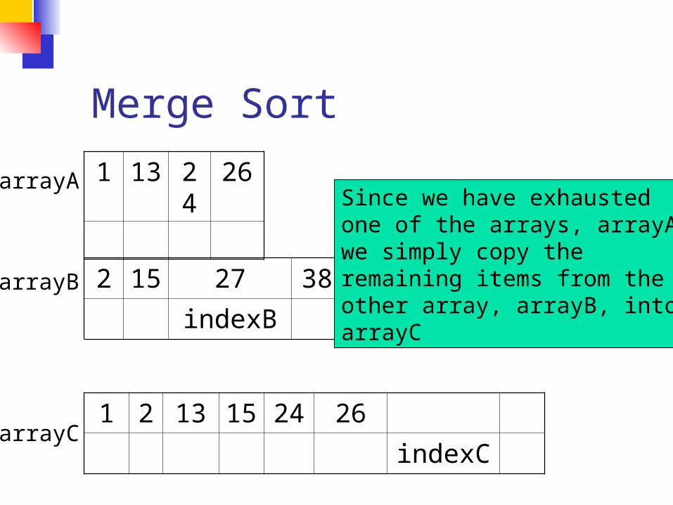
Merge Sort
1 13 24
26
1 2 13 15 24 26indexC
arrayA
2 15 27 38indexB
arrayB
arrayC
Since we have exhaustedone of the arrays arrayAwe simply copy the remaining items from theother array arrayB intoarrayC
Merge Sort
1 13 24
26
1 2 13 15 24 26 27 38
arrayA
2 15 27 38arrayB
arrayC
Efficiency Summary
Sort Worst Case Average Case
Insertion O(n2) O(n2)
Shell O(n15) O(n125)
Selection O(n2) O(n2)
Bubble O(n2) O(n2)
Quick O(n2) O(nlog2n)
Heap O(nlog2n) O(nlog2n)
Merge O(nlog2n) O(nlog2n)
More Sorting
radix sort bucket sort in-place sorting how fast can we sort
Radix Sort
Unlike other sorting methods radix sort considers the structure of the keys
Assume keys are represented in a base M number system (M = radix) ie if M = 2 the keys are represented in binary
Sorting is done by comparing bits in the same position
Extension to keys that are alphanumeric strings
Radix Exchange Sort
Examine bits from left to right1 Sort array with respect to leftmost bit
2 Partition array
3Recursionrecursively sort top subarray ignoring leftmost bitrecursively sort bottom subarray ignoring leftmost bit
Time to sort n b-bit numbers O(b n)
Radix Exchange SortHow do we do the sort from the previous page Same idea as partition in Quicksort repeat
scan top-down to find key starting with 1scan bottom-up to find key starting with 0exchange keys
until scan indices cross
Radix Exchange Sort
Radix Exchange Sort vs Quicksort
Similaritiesboth partition arrayboth recursively sort sub-arrays
DifferencesMethod of partitioning
radix exchange divides array based on greater than or less than 2b-1
quicksort partitions based on greater than or less than some element of the array
Time complexityRadix exchange O (bn)Quicksort average case O (n log n)
Straight Radix Sort
Examines bits from right to left
for k = 0 to b-1 sort the array in a stable waylooking only at bit k
Note order of these bits after sort
Recall ldquosort in a stable
wayrdquo
In a stable sort the initial relative order of equal keys is unchangedFor example observe the first step of the sort from the previous page
Note that the relative order of those keys ending with 0 is unchanged and the same is true for elements ending in 1
The Algorithm is Correct (right)
We show that any two keys are in the correct relative order at the end of the algorithm
Given two keys let k be the leftmost bit-position where they differ
At step k the two keys are put in the correct relative orderBecause of stability the successive steps do not change the relative order of the two keys
For InstanceConsider a sort on an array with these two keys
Radix sorting can be applied to decimal numbers
Straight Radix SortTime Complexity
for k = 0 to b - 1 sort the array in a stable way looking only at bit k
Suppose we can perform the stable sort above in O(n) time The total time complexity would be
O(bn)As you might have guessed we can perform a stable sort based on the keysrsquo kth digit in O(n) time
The method you ask Why itrsquos Bucket Sort of course
Bucket Sort
BASICSn numbersEach number 1 2 3 mStableTime O (n + m)
For example m = 3 and our array is
(note that there are two ldquo2rdquos and two ldquo1rdquos)
First we create M ldquobucketsrdquo
Bucket SortEach element of the array is put in one of the m ldquobucketsrdquo
Bucket Sort
Now pull the elements from the buckets into the array
At last the sorted array (sorted in a stable way)
Comparison Sorting Elements are rearranged by comparing
values of keys Comparison of keys is interleaved with
rearrangements of the order of various pairs of keys as the algorithm progressively moves keys into final sorted order
Comparisons performed at given stage will depend on outcomes of previous comparisons and previous rearrangements of keys
Sorting an array of 3 elements a b and c produces 6 or 3 distinct orderings
Decision TreeConsider a decision tree that sorts n items The next slide shows a decision tree for 3 items a b c
Ovals represent comparisons If lt we traverse down a left branch
otherwise a right branch
Decision Tree on 3 Elements
a b c
bltc
bltc
altb
altc altc
a c b b a cc a b
c b a
b c a
true
true
true true
true
false
false
false
false
false
Levels in Decision Trees Number the levels starting at zero Level i can represent 2i arrangements Our decision tree can represent 8 = 23
arrangements If we have 4 items then 4 = 24 elements
but 4 levels gives at most 24 = 16 so we need 5 levels since 25 = 32 24
If we have k arrangements to represent then we need a decision tree with at least lg k levels
Size of Decision TreeWhen dealing with n elements we have n
possible arrangements and need a decision tree with at least lg n levels
)lg(2
lg2
2lg
2
)2lg()1lg(lg
)1lg()2lg()2lg()1lg(lg
))1)(2)(2)(1(lg()lg(
nn
nn
n
nn
nnn
nnn
nnnn
Lower Bound Resultn = n(n-1)(n-2)hellip21
from this we getlg(n) = lg(n) + lg(n-1) + lg(n-2) +hellip+
lg2 + lg1this means
lg(n) lt nlg(n)and the two results together show
O(lg(n)) = O(nlg(n))
No general sorting algorithm can run faster than O(n lg n)
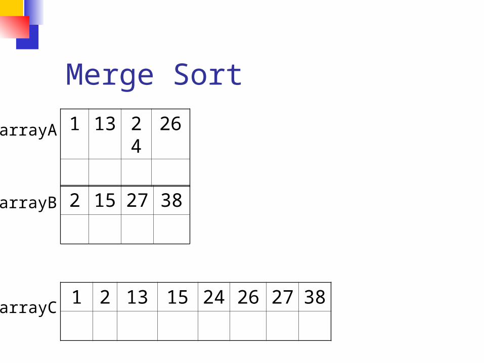
Merge Sort
1 13 24
26
1 2 13 15 24 26 27 38
arrayA
2 15 27 38arrayB
arrayC
Efficiency Summary
Sort Worst Case Average Case
Insertion O(n2) O(n2)
Shell O(n15) O(n125)
Selection O(n2) O(n2)
Bubble O(n2) O(n2)
Quick O(n2) O(nlog2n)
Heap O(nlog2n) O(nlog2n)
Merge O(nlog2n) O(nlog2n)
More Sorting
radix sort bucket sort in-place sorting how fast can we sort
Radix Sort
Unlike other sorting methods radix sort considers the structure of the keys
Assume keys are represented in a base M number system (M = radix) ie if M = 2 the keys are represented in binary
Sorting is done by comparing bits in the same position
Extension to keys that are alphanumeric strings
Radix Exchange Sort
Examine bits from left to right1 Sort array with respect to leftmost bit
2 Partition array
3Recursionrecursively sort top subarray ignoring leftmost bitrecursively sort bottom subarray ignoring leftmost bit
Time to sort n b-bit numbers O(b n)
Radix Exchange SortHow do we do the sort from the previous page Same idea as partition in Quicksort repeat
scan top-down to find key starting with 1scan bottom-up to find key starting with 0exchange keys
until scan indices cross
Radix Exchange Sort
Radix Exchange Sort vs Quicksort
Similaritiesboth partition arrayboth recursively sort sub-arrays
DifferencesMethod of partitioning
radix exchange divides array based on greater than or less than 2b-1
quicksort partitions based on greater than or less than some element of the array
Time complexityRadix exchange O (bn)Quicksort average case O (n log n)
Straight Radix Sort
Examines bits from right to left
for k = 0 to b-1 sort the array in a stable waylooking only at bit k
Note order of these bits after sort
Recall ldquosort in a stable
wayrdquo
In a stable sort the initial relative order of equal keys is unchangedFor example observe the first step of the sort from the previous page
Note that the relative order of those keys ending with 0 is unchanged and the same is true for elements ending in 1
The Algorithm is Correct (right)
We show that any two keys are in the correct relative order at the end of the algorithm
Given two keys let k be the leftmost bit-position where they differ
At step k the two keys are put in the correct relative orderBecause of stability the successive steps do not change the relative order of the two keys
For InstanceConsider a sort on an array with these two keys
Radix sorting can be applied to decimal numbers
Straight Radix SortTime Complexity
for k = 0 to b - 1 sort the array in a stable way looking only at bit k
Suppose we can perform the stable sort above in O(n) time The total time complexity would be
O(bn)As you might have guessed we can perform a stable sort based on the keysrsquo kth digit in O(n) time
The method you ask Why itrsquos Bucket Sort of course
Bucket Sort
BASICSn numbersEach number 1 2 3 mStableTime O (n + m)
For example m = 3 and our array is
(note that there are two ldquo2rdquos and two ldquo1rdquos)
First we create M ldquobucketsrdquo
Bucket SortEach element of the array is put in one of the m ldquobucketsrdquo
Bucket Sort
Now pull the elements from the buckets into the array
At last the sorted array (sorted in a stable way)
Comparison Sorting Elements are rearranged by comparing
values of keys Comparison of keys is interleaved with
rearrangements of the order of various pairs of keys as the algorithm progressively moves keys into final sorted order
Comparisons performed at given stage will depend on outcomes of previous comparisons and previous rearrangements of keys
Sorting an array of 3 elements a b and c produces 6 or 3 distinct orderings
Decision TreeConsider a decision tree that sorts n items The next slide shows a decision tree for 3 items a b c
Ovals represent comparisons If lt we traverse down a left branch
otherwise a right branch
Decision Tree on 3 Elements
a b c
bltc
bltc
altb
altc altc
a c b b a cc a b
c b a
b c a
true
true
true true
true
false
false
false
false
false
Levels in Decision Trees Number the levels starting at zero Level i can represent 2i arrangements Our decision tree can represent 8 = 23
arrangements If we have 4 items then 4 = 24 elements
but 4 levels gives at most 24 = 16 so we need 5 levels since 25 = 32 24
If we have k arrangements to represent then we need a decision tree with at least lg k levels
Size of Decision TreeWhen dealing with n elements we have n
possible arrangements and need a decision tree with at least lg n levels
)lg(2
lg2
2lg
2
)2lg()1lg(lg
)1lg()2lg()2lg()1lg(lg
))1)(2)(2)(1(lg()lg(
nn
nn
n
nn
nnn
nnn
nnnn
Lower Bound Resultn = n(n-1)(n-2)hellip21
from this we getlg(n) = lg(n) + lg(n-1) + lg(n-2) +hellip+
lg2 + lg1this means
lg(n) lt nlg(n)and the two results together show
O(lg(n)) = O(nlg(n))
No general sorting algorithm can run faster than O(n lg n)
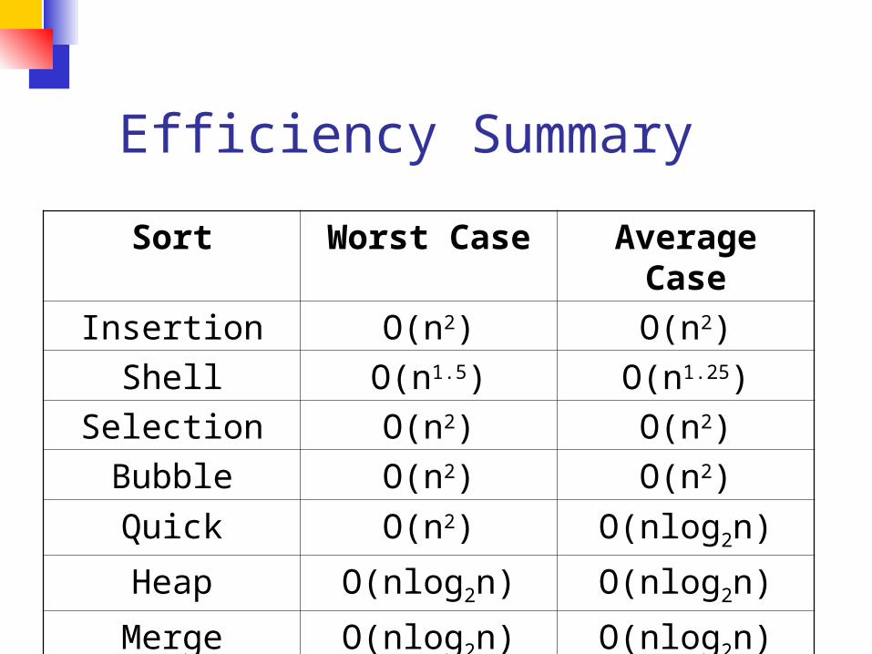
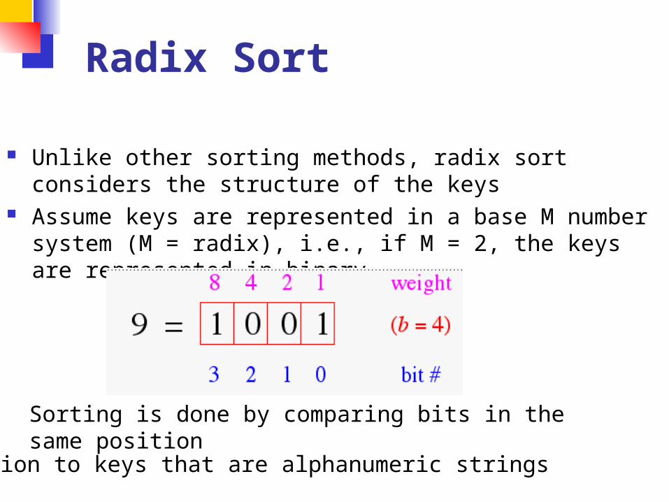
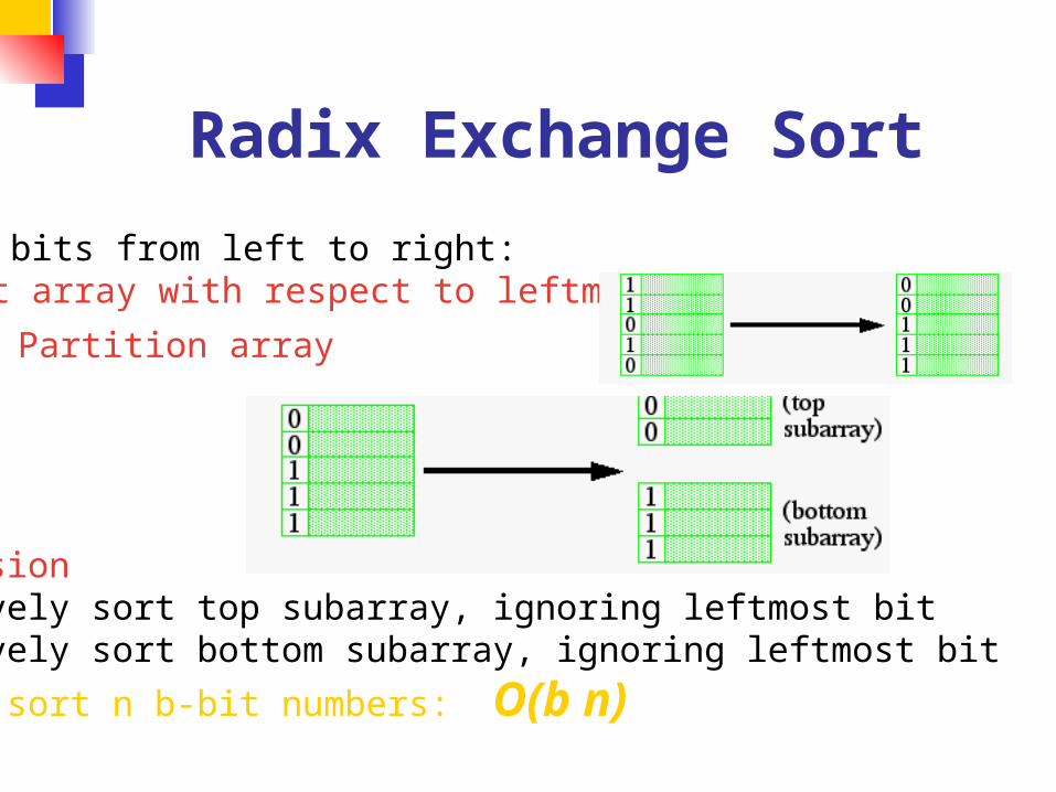
Radix Exchange Sort
Examine bits from left to right1 Sort array with respect to leftmost bit
2 Partition array
3Recursionrecursively sort top subarray ignoring leftmost bitrecursively sort bottom subarray ignoring leftmost bit
Time to sort n b-bit numbers O(b n)
Radix Exchange SortHow do we do the sort from the previous page Same idea as partition in Quicksort repeat
scan top-down to find key starting with 1scan bottom-up to find key starting with 0exchange keys
until scan indices cross
Radix Exchange Sort
Radix Exchange Sort vs Quicksort
Similaritiesboth partition arrayboth recursively sort sub-arrays
DifferencesMethod of partitioning
radix exchange divides array based on greater than or less than 2b-1
quicksort partitions based on greater than or less than some element of the array
Time complexityRadix exchange O (bn)Quicksort average case O (n log n)
Straight Radix Sort
Examines bits from right to left
for k = 0 to b-1 sort the array in a stable waylooking only at bit k
Note order of these bits after sort
Recall ldquosort in a stable
wayrdquo
In a stable sort the initial relative order of equal keys is unchangedFor example observe the first step of the sort from the previous page
Note that the relative order of those keys ending with 0 is unchanged and the same is true for elements ending in 1
The Algorithm is Correct (right)
We show that any two keys are in the correct relative order at the end of the algorithm
Given two keys let k be the leftmost bit-position where they differ
At step k the two keys are put in the correct relative orderBecause of stability the successive steps do not change the relative order of the two keys
For InstanceConsider a sort on an array with these two keys
Radix sorting can be applied to decimal numbers
Straight Radix SortTime Complexity
for k = 0 to b - 1 sort the array in a stable way looking only at bit k
Suppose we can perform the stable sort above in O(n) time The total time complexity would be
O(bn)As you might have guessed we can perform a stable sort based on the keysrsquo kth digit in O(n) time
The method you ask Why itrsquos Bucket Sort of course
Bucket Sort
BASICSn numbersEach number 1 2 3 mStableTime O (n + m)
For example m = 3 and our array is
(note that there are two ldquo2rdquos and two ldquo1rdquos)
First we create M ldquobucketsrdquo
Bucket SortEach element of the array is put in one of the m ldquobucketsrdquo
Bucket Sort
Now pull the elements from the buckets into the array
At last the sorted array (sorted in a stable way)
Comparison Sorting Elements are rearranged by comparing
values of keys Comparison of keys is interleaved with
rearrangements of the order of various pairs of keys as the algorithm progressively moves keys into final sorted order
Comparisons performed at given stage will depend on outcomes of previous comparisons and previous rearrangements of keys
Sorting an array of 3 elements a b and c produces 6 or 3 distinct orderings
Decision TreeConsider a decision tree that sorts n items The next slide shows a decision tree for 3 items a b c
Ovals represent comparisons If lt we traverse down a left branch
otherwise a right branch
Decision Tree on 3 Elements
a b c
bltc
bltc
altb
altc altc
a c b b a cc a b
c b a
b c a
true
true
true true
true
false
false
false
false
false
Levels in Decision Trees Number the levels starting at zero Level i can represent 2i arrangements Our decision tree can represent 8 = 23
arrangements If we have 4 items then 4 = 24 elements
but 4 levels gives at most 24 = 16 so we need 5 levels since 25 = 32 24
If we have k arrangements to represent then we need a decision tree with at least lg k levels
Size of Decision TreeWhen dealing with n elements we have n
possible arrangements and need a decision tree with at least lg n levels
)lg(2
lg2
2lg
2
)2lg()1lg(lg
)1lg()2lg()2lg()1lg(lg
))1)(2)(2)(1(lg()lg(
nn
nn
n
nn
nnn
nnn
nnnn
Lower Bound Resultn = n(n-1)(n-2)hellip21
from this we getlg(n) = lg(n) + lg(n-1) + lg(n-2) +hellip+
lg2 + lg1this means
lg(n) lt nlg(n)and the two results together show
O(lg(n)) = O(nlg(n))
No general sorting algorithm can run faster than O(n lg n)
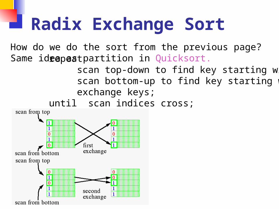
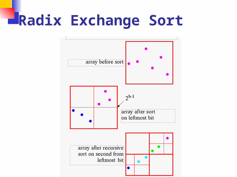
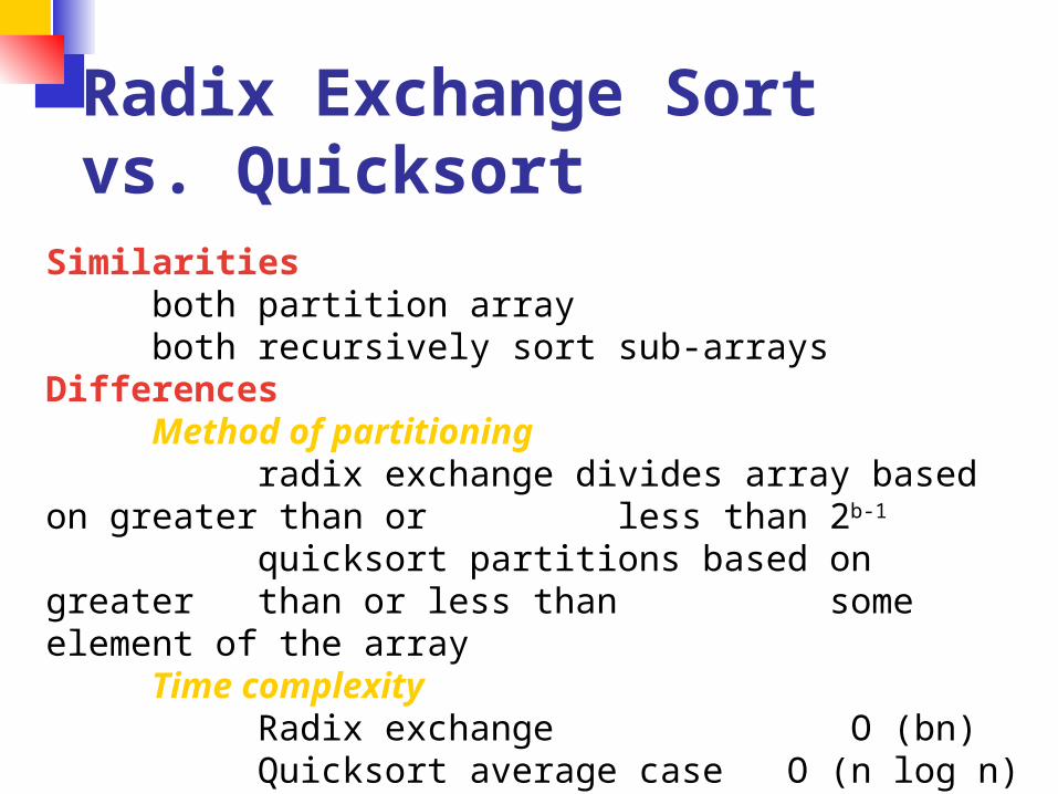
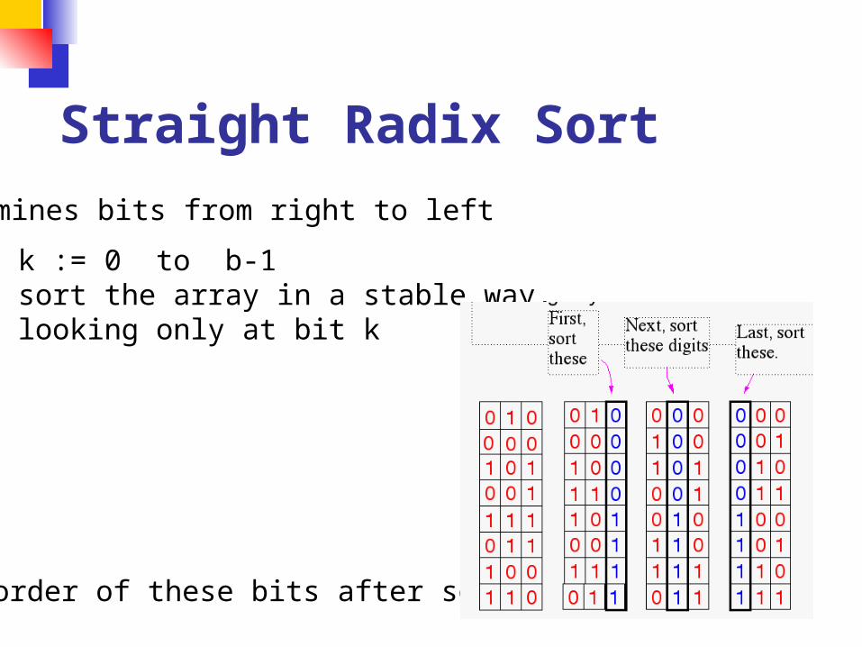
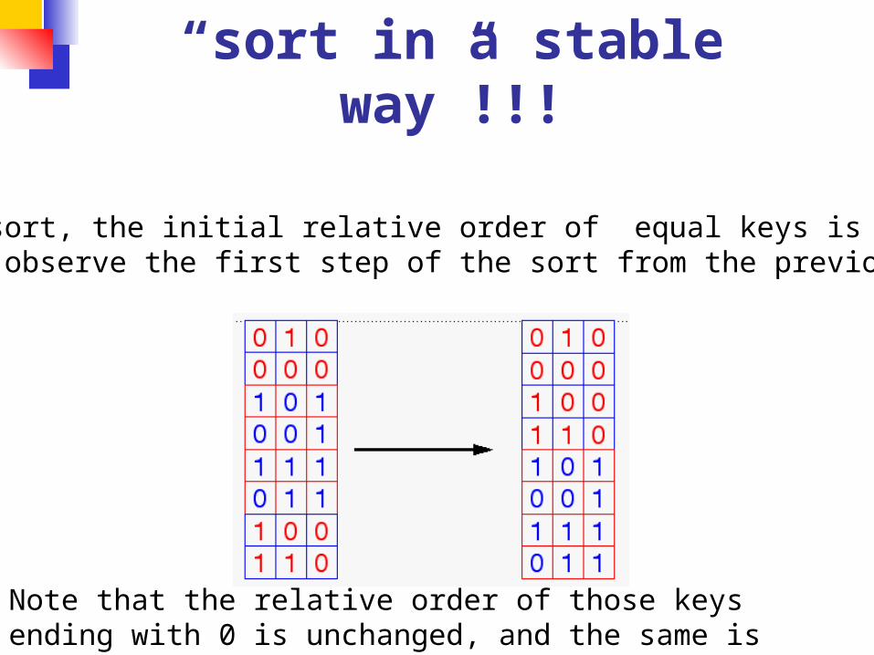
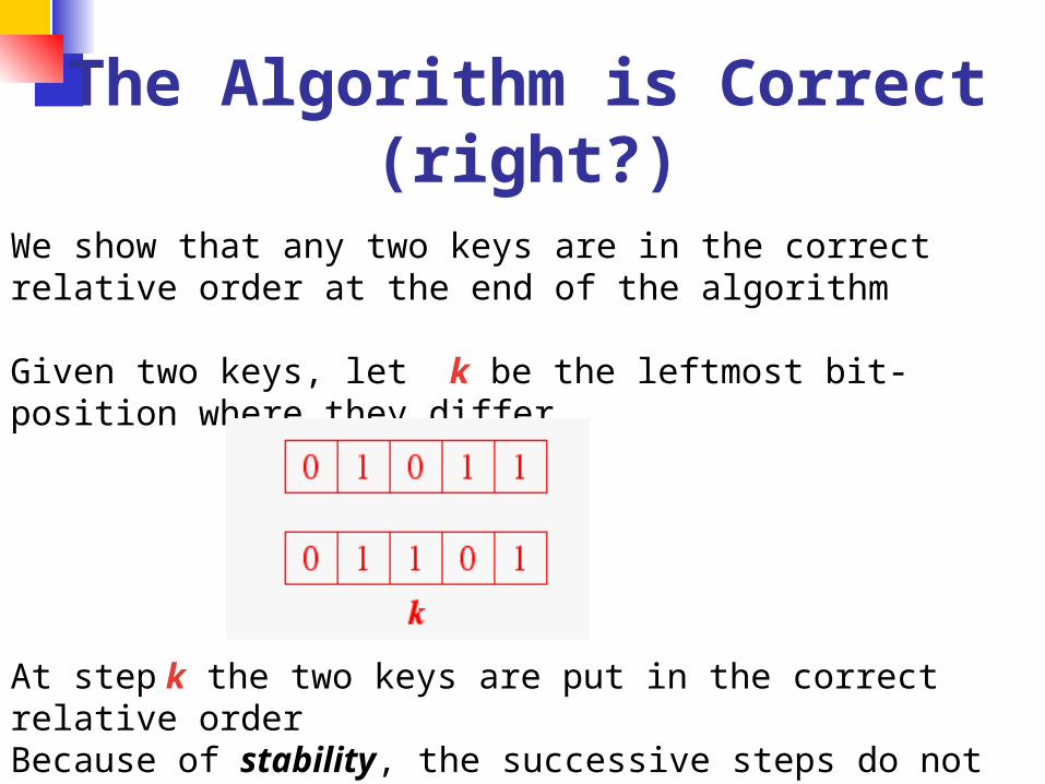
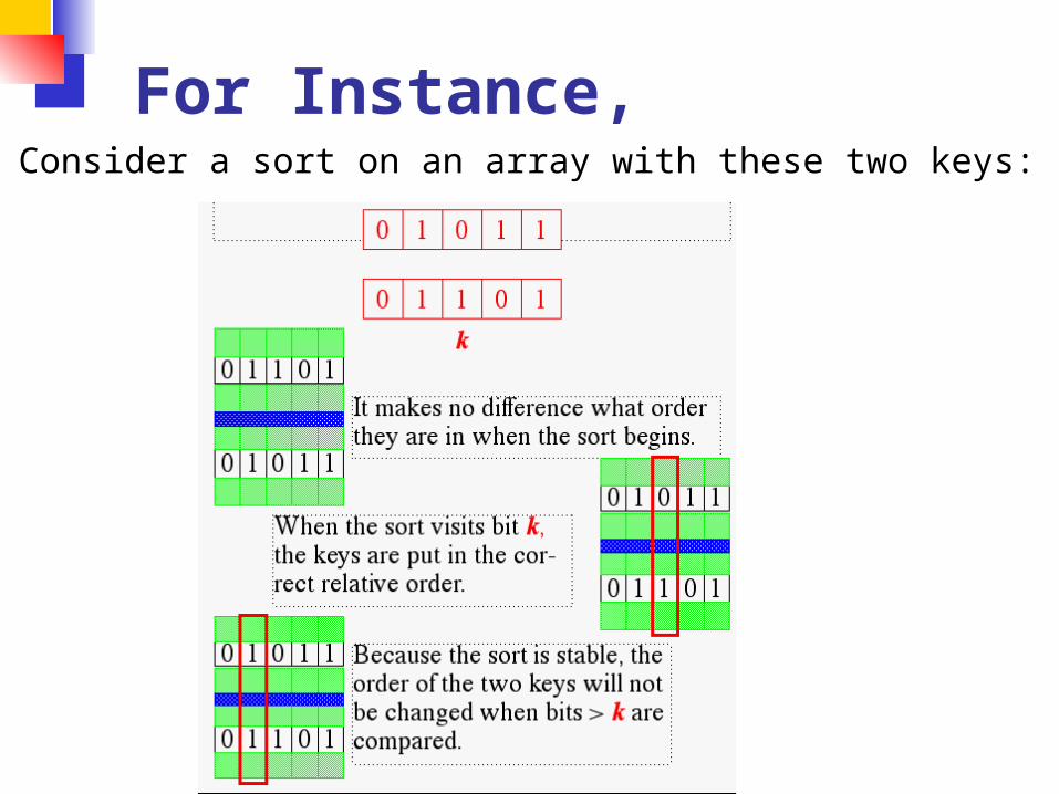
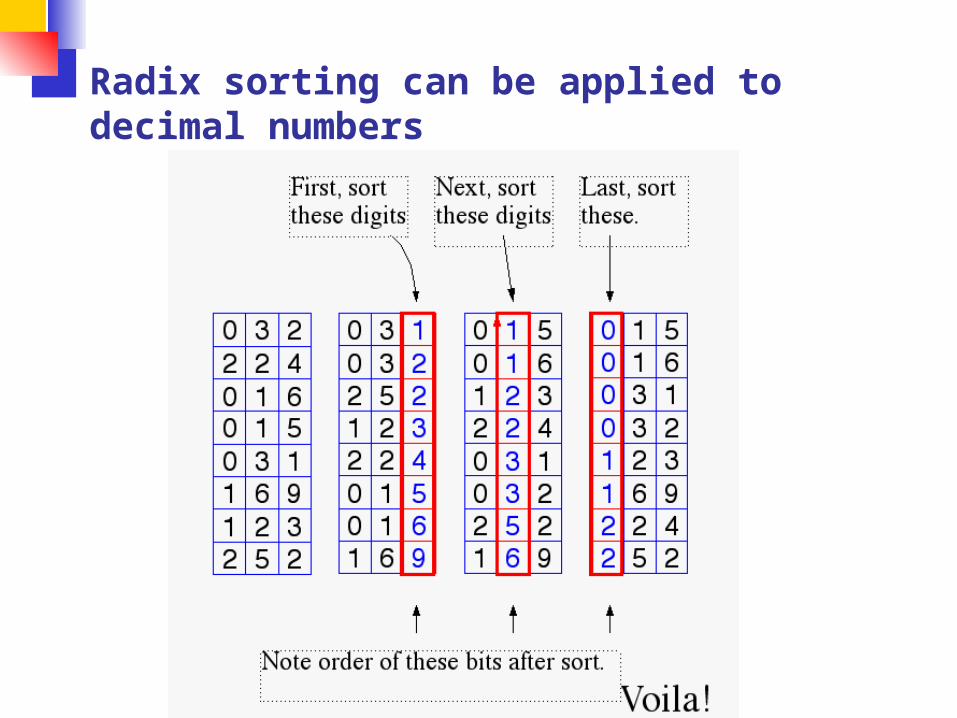
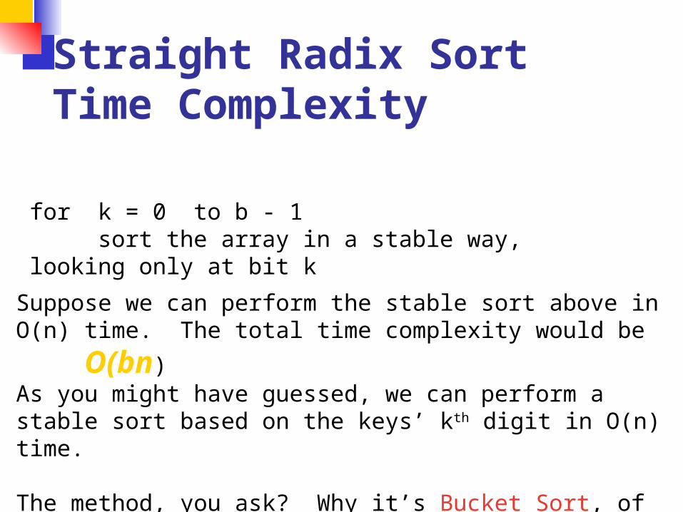
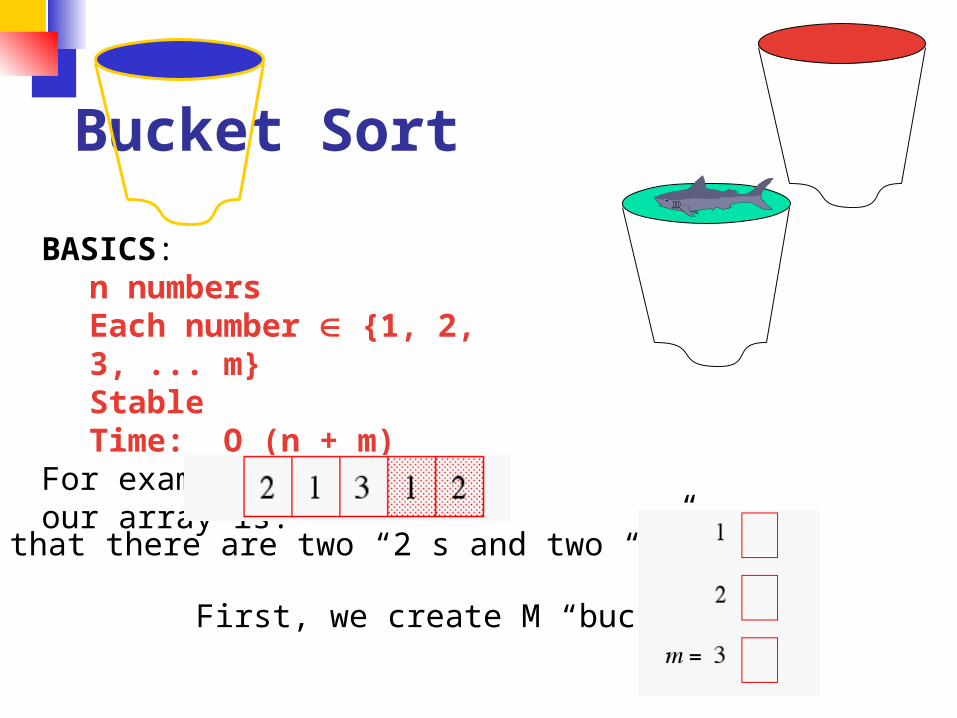
Bucket Sort
BASICSn numbersEach number 1 2 3 mStableTime O (n + m)
For example m = 3 and our array is
(note that there are two ldquo2rdquos and two ldquo1rdquos)
First we create M ldquobucketsrdquo
Bucket SortEach element of the array is put in one of the m ldquobucketsrdquo
Bucket Sort
Now pull the elements from the buckets into the array
At last the sorted array (sorted in a stable way)
Comparison Sorting Elements are rearranged by comparing
values of keys Comparison of keys is interleaved with
rearrangements of the order of various pairs of keys as the algorithm progressively moves keys into final sorted order
Comparisons performed at given stage will depend on outcomes of previous comparisons and previous rearrangements of keys
Sorting an array of 3 elements a b and c produces 6 or 3 distinct orderings
Decision TreeConsider a decision tree that sorts n items The next slide shows a decision tree for 3 items a b c
Ovals represent comparisons If lt we traverse down a left branch
otherwise a right branch
Decision Tree on 3 Elements
a b c
bltc
bltc
altb
altc altc
a c b b a cc a b
c b a
b c a
true
true
true true
true
false
false
false
false
false
Levels in Decision Trees Number the levels starting at zero Level i can represent 2i arrangements Our decision tree can represent 8 = 23
arrangements If we have 4 items then 4 = 24 elements
but 4 levels gives at most 24 = 16 so we need 5 levels since 25 = 32 24
If we have k arrangements to represent then we need a decision tree with at least lg k levels
Size of Decision TreeWhen dealing with n elements we have n
possible arrangements and need a decision tree with at least lg n levels
)lg(2
lg2
2lg
2
)2lg()1lg(lg
)1lg()2lg()2lg()1lg(lg
))1)(2)(2)(1(lg()lg(
nn
nn
n
nn
nnn
nnn
nnnn
Lower Bound Resultn = n(n-1)(n-2)hellip21
from this we getlg(n) = lg(n) + lg(n-1) + lg(n-2) +hellip+
lg2 + lg1this means
lg(n) lt nlg(n)and the two results together show
O(lg(n)) = O(nlg(n))
No general sorting algorithm can run faster than O(n lg n)
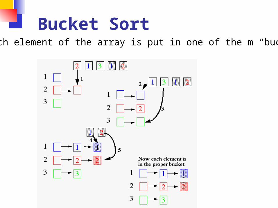
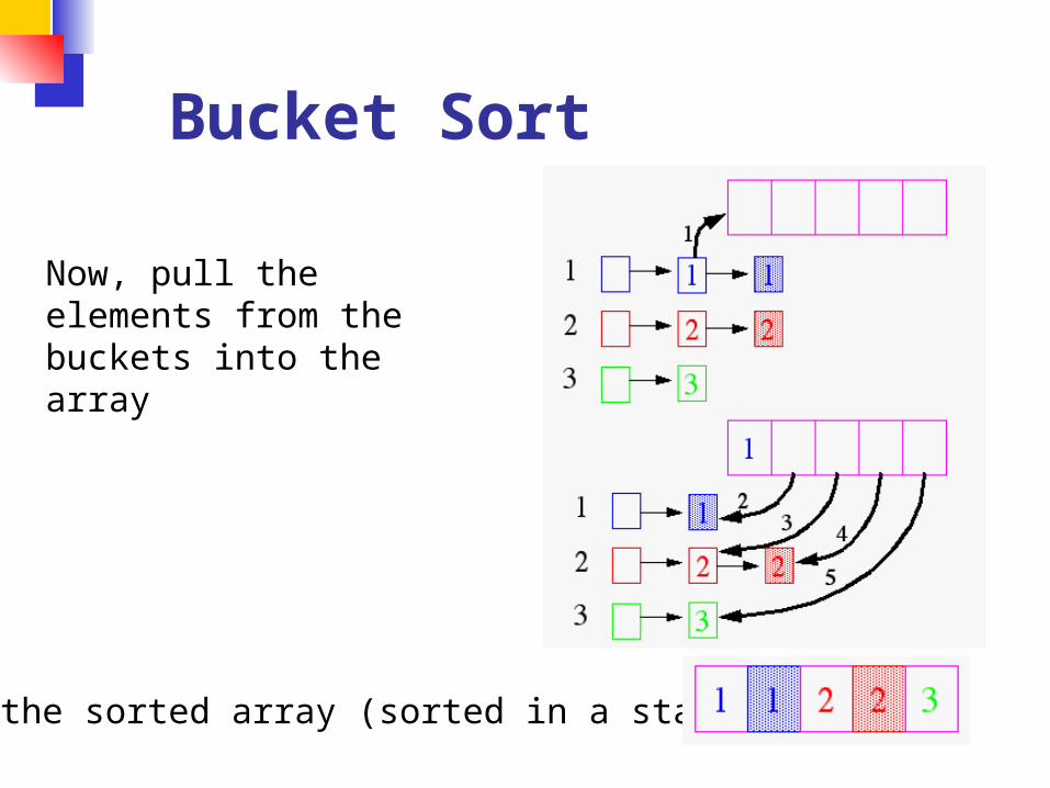
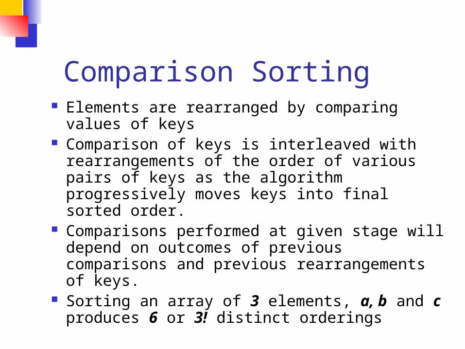
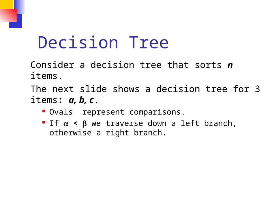
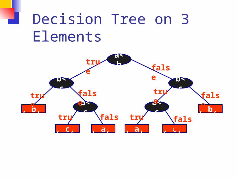
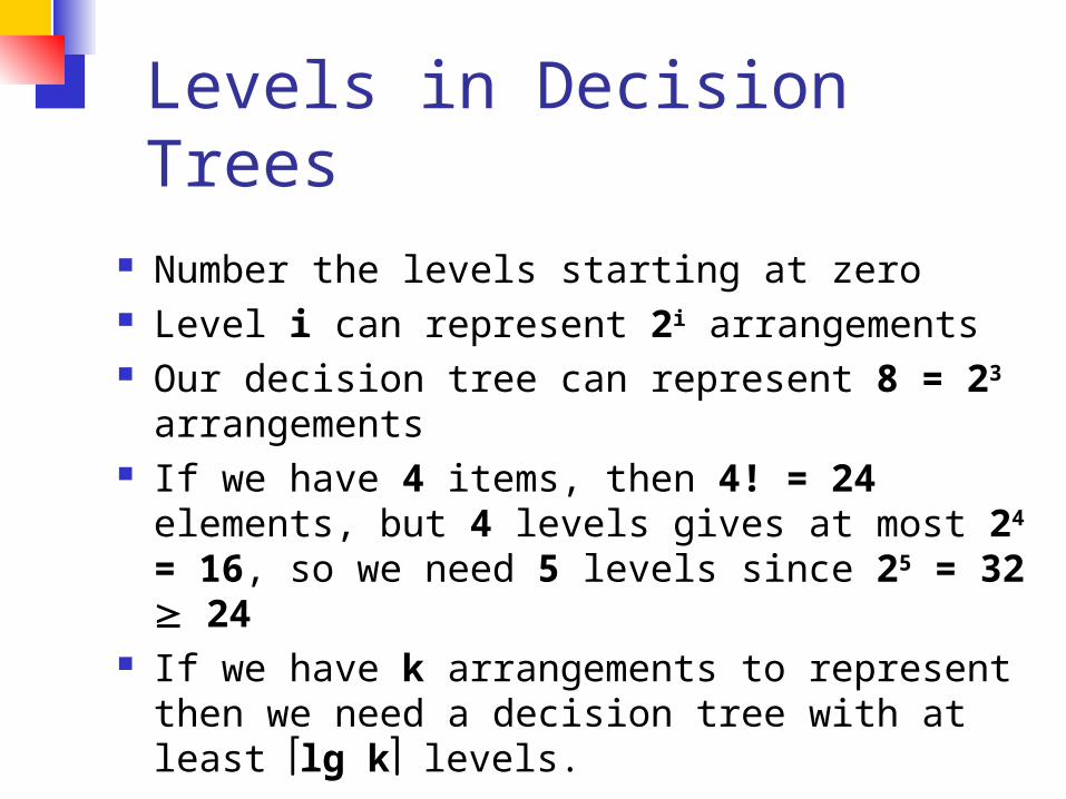
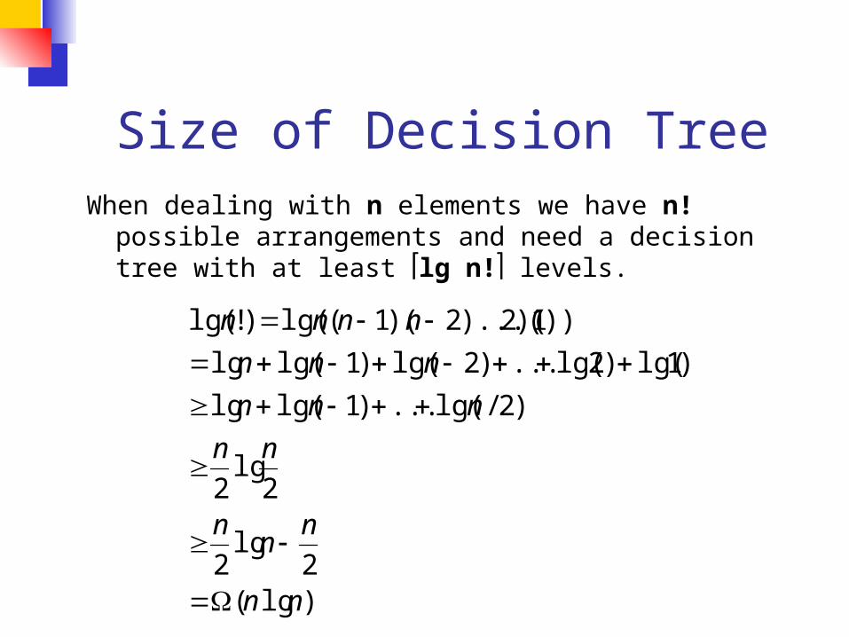
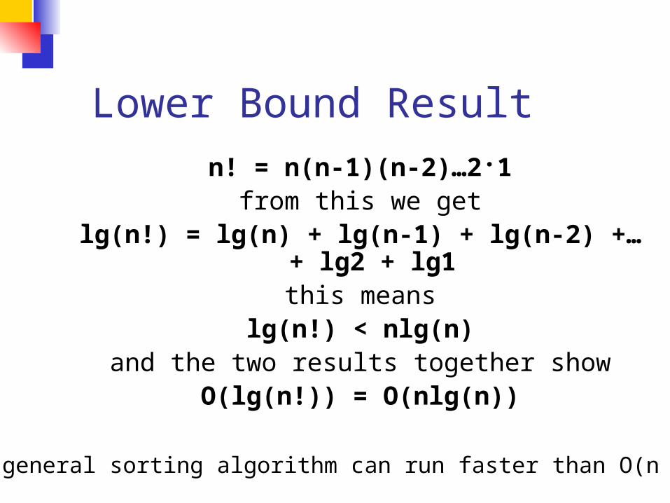
Lower Bound Resultn = n(n-1)(n-2)hellip21
from this we getlg(n) = lg(n) + lg(n-1) + lg(n-2) +hellip+
lg2 + lg1this means
lg(n) lt nlg(n)and the two results together show
O(lg(n)) = O(nlg(n))
No general sorting algorithm can run faster than O(n lg n)
Top Related