In general, we can just represent a bone by its transformation without consider the hierarchy. This is more flexible while still giving the same skin deformation.
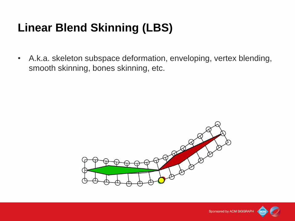
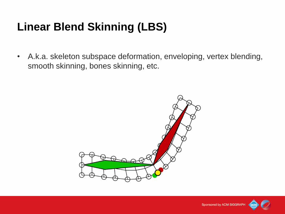
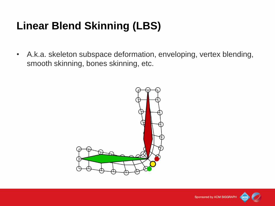
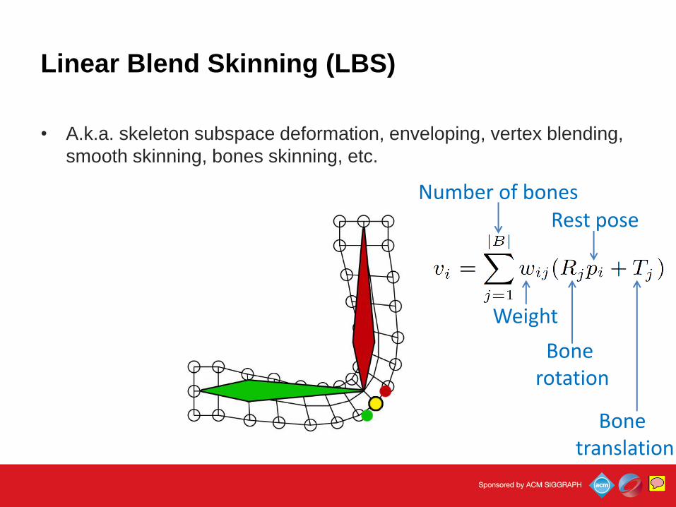
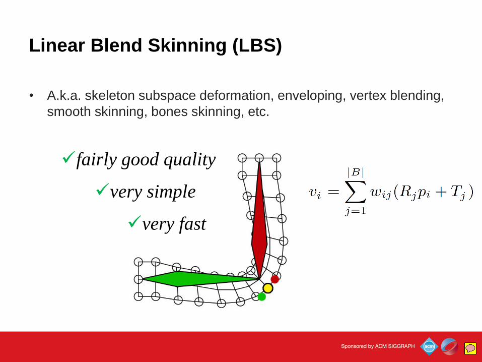
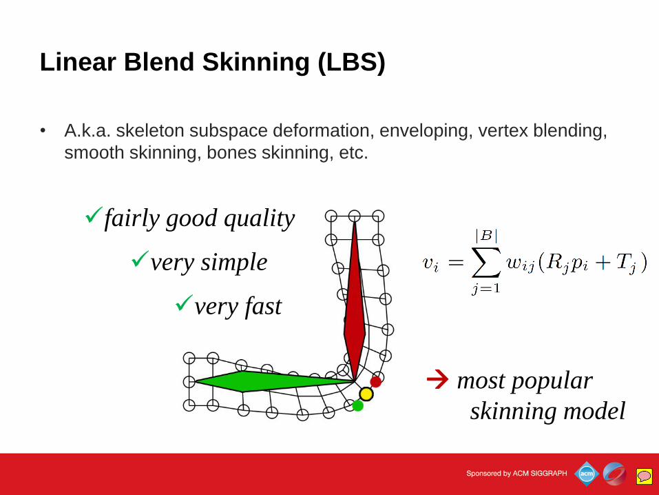
So, LBS is the most popular skinning model, especially for real time applications such as games.
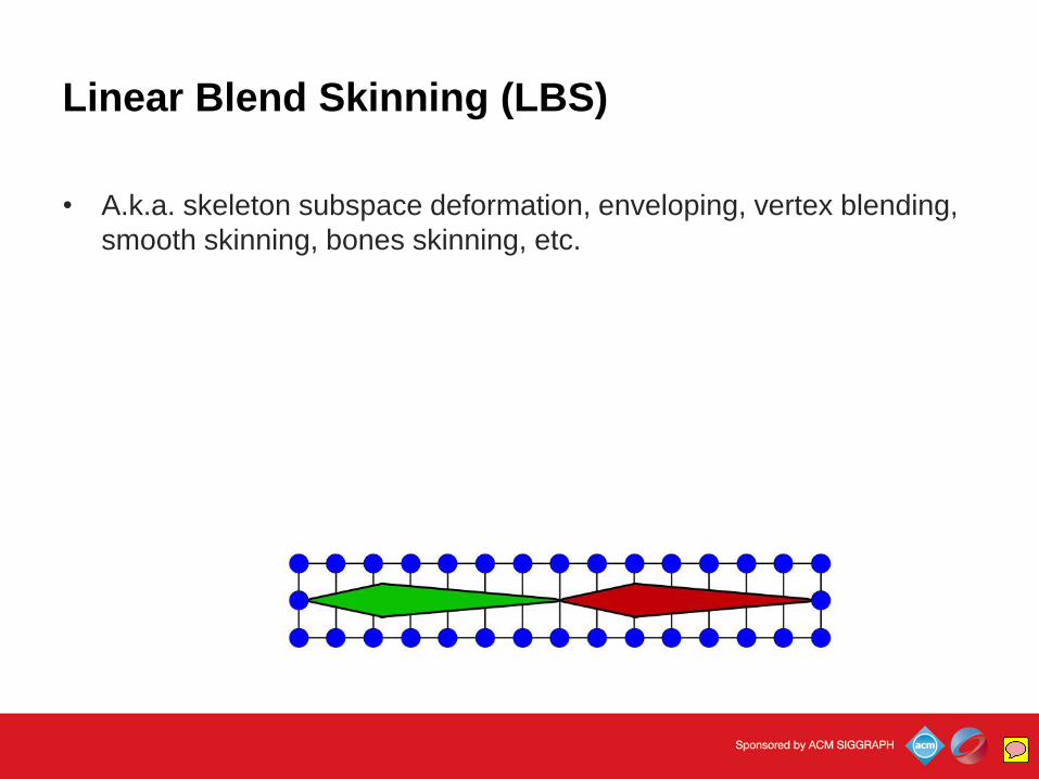
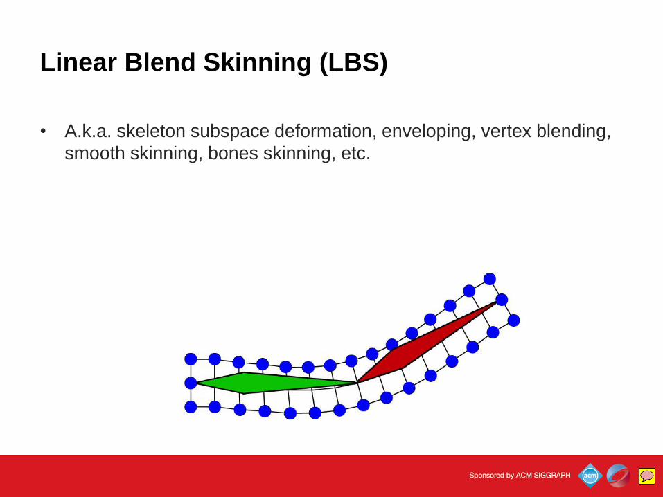
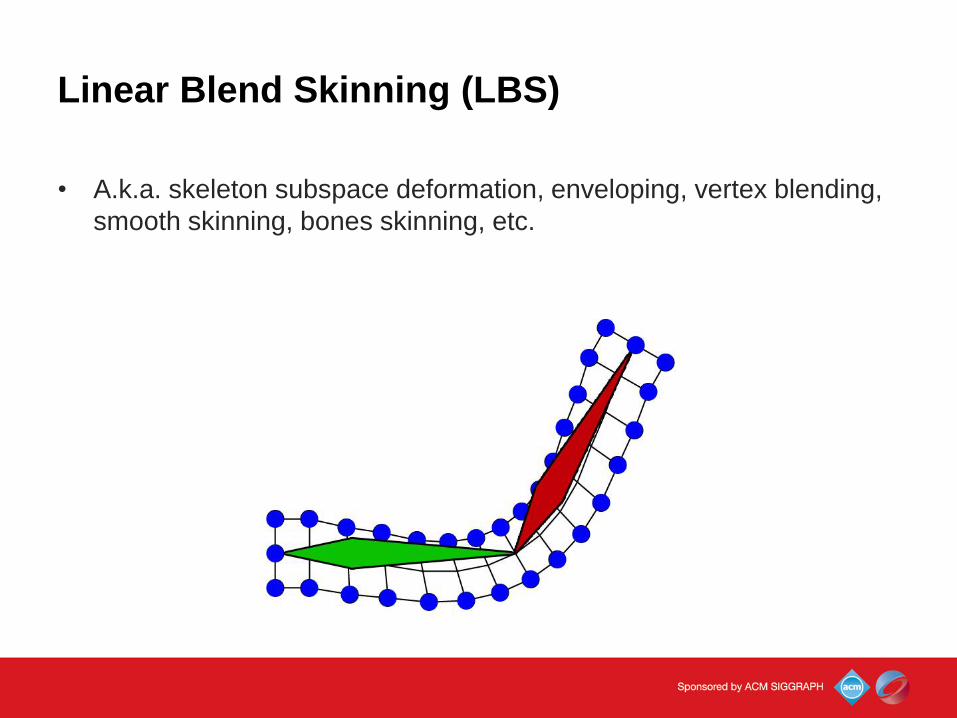
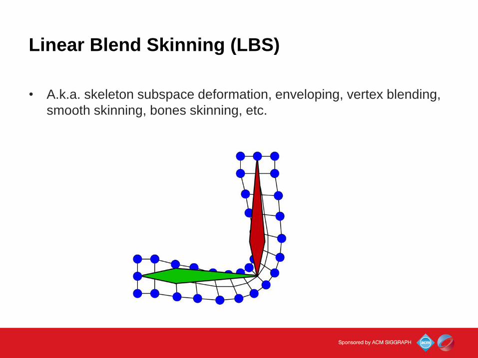
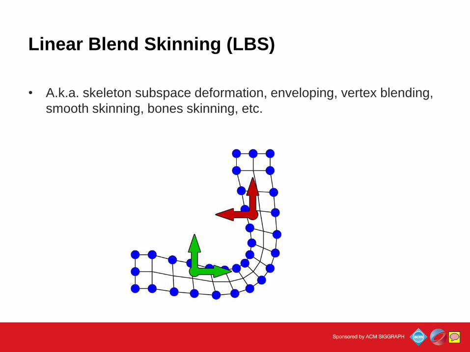
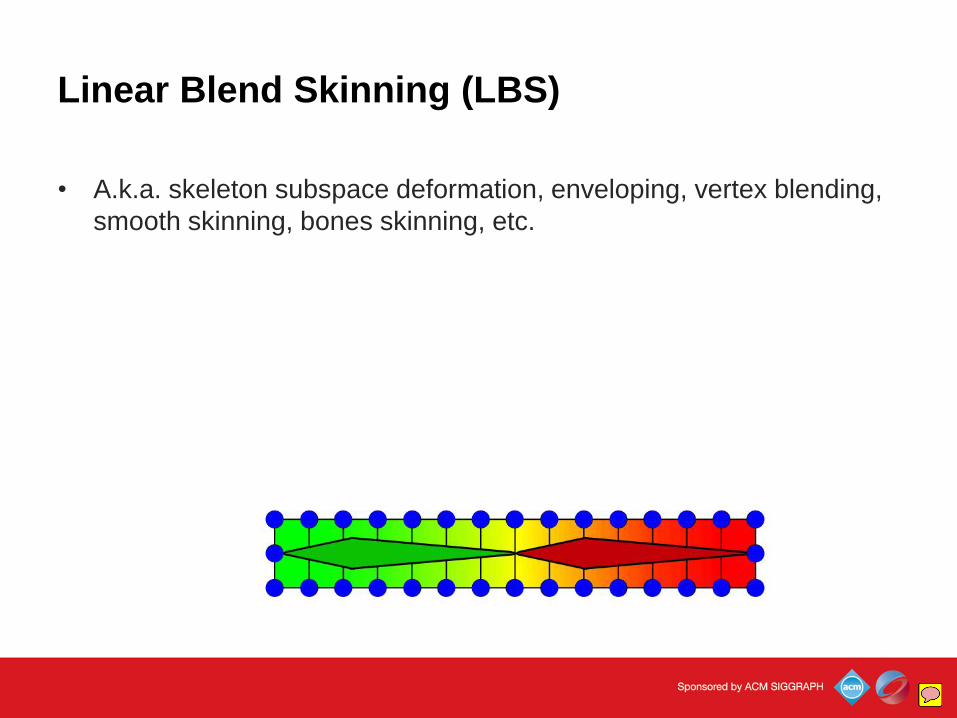
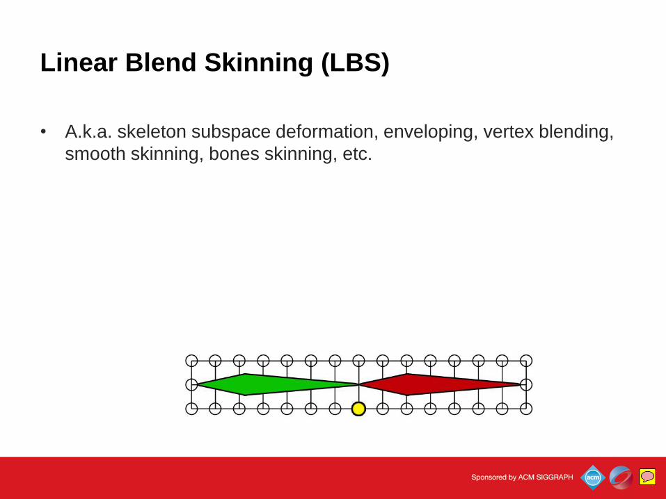
Linear Blend Skinning (LBS)
BinhLe
Sticky Note
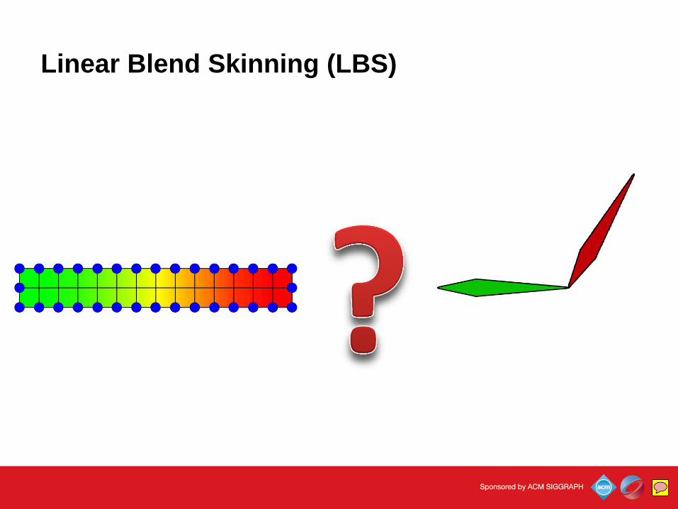
To setup the LBS, we naturally come up with two questions: - How to get the skinning weights? - and how to control the bone transformations?
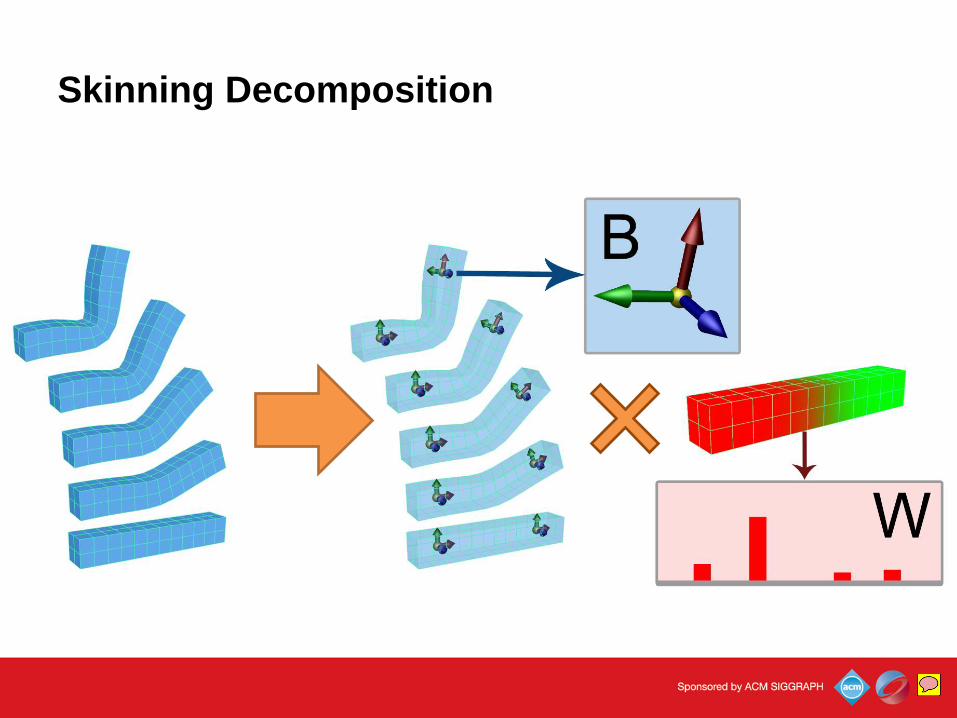
Skinning Decomposition
BinhLe
Sticky Note
Beside manual solutions for above questions, we can do it with Skinning Decomposition…
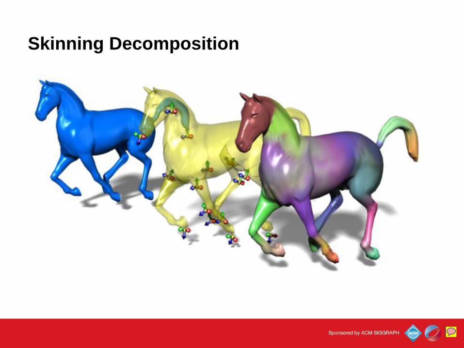
Skinning Decomposition
BinhLe
Sticky Note
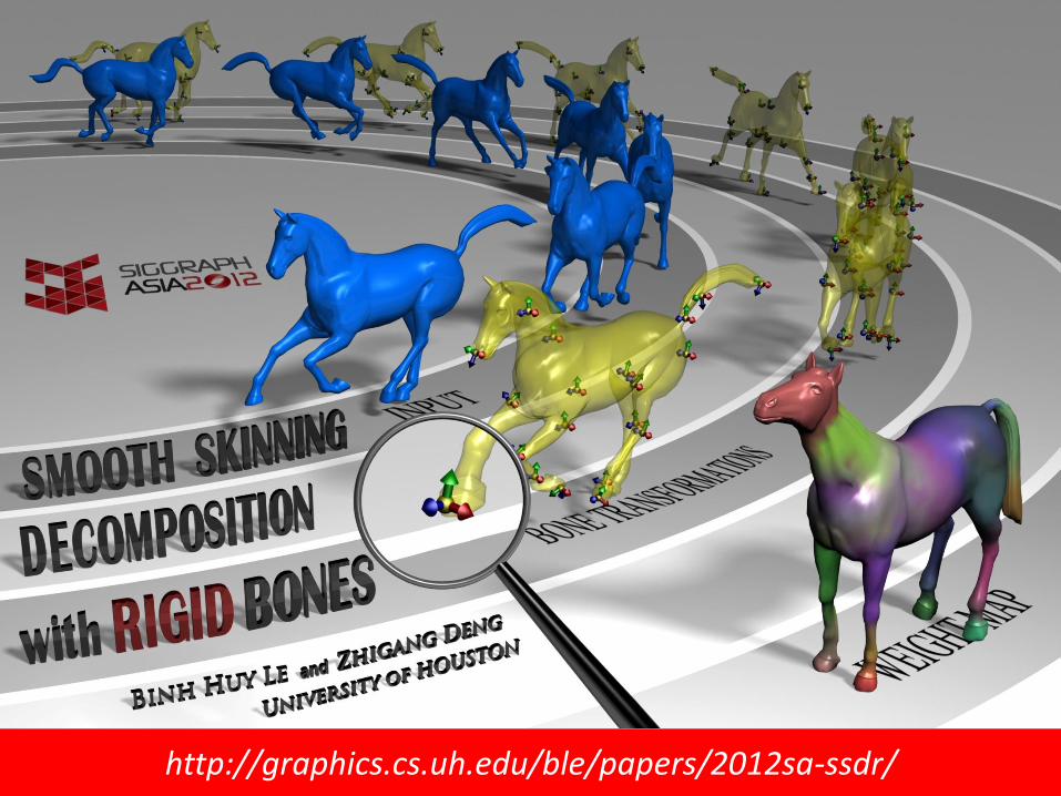
…where input example poses is decomposed into bone transformations (which is denoted by B here) and skinning weights (which is denoted by W).
Skinning Decomposition
BinhLe
Sticky Note
For example, here we decompose the horse animated mesh sequence into the bone transformations and weight map.
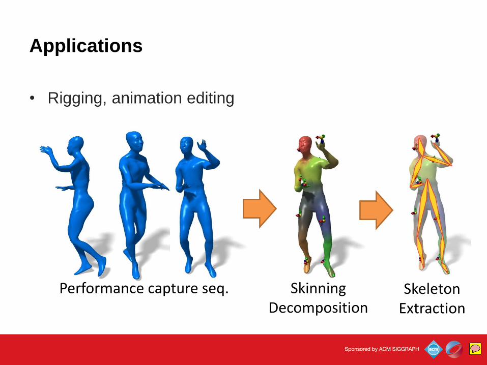
Applications
• Rigging, animation editing
Performance capture seq. Skinning Decomposition
Skeleton Extraction
BinhLe
Sticky Note
If we can solve the Skinning Decomposition problem, we can apply it for some tasks. For example, rigging and editing the performance capture mesh sequences.
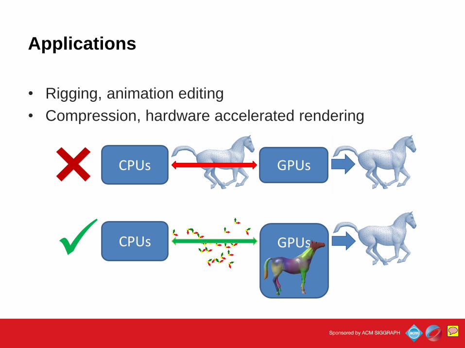
Applications
• Rigging, animation editing
• Compression, hardware accelerated rendering
CPUs GPUs
CPUs GPUs
BinhLe
Sticky Note
Or you can compress an animated mesh sequence to save the bandwidth between CPUs and GPUs.
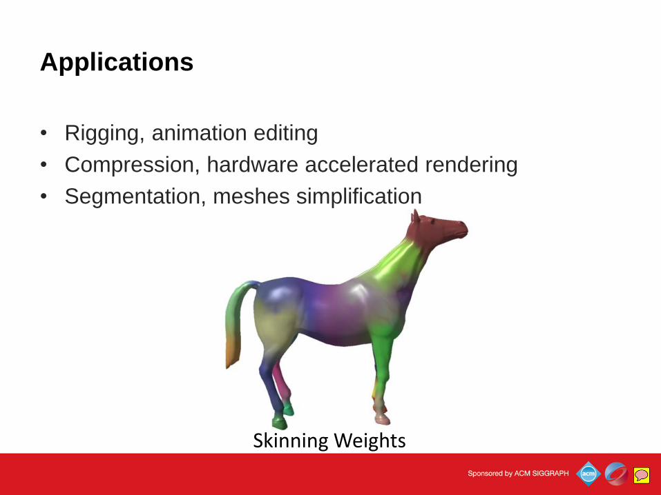
Applications
• Rigging, animation editing
• Compression, hardware accelerated rendering
• Segmentation, meshes simplification
Skinning Weights
BinhLe
Sticky Note
The skinning weights can also help you with segmentations or simplification tasks.
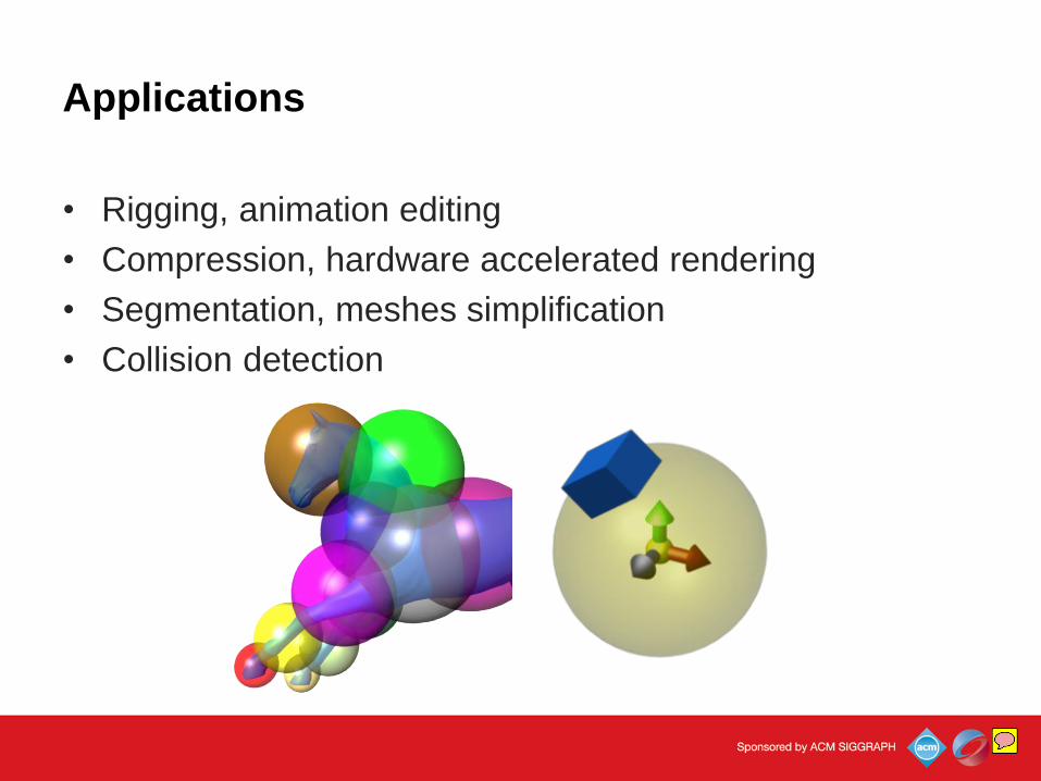
Applications
• Rigging, animation editing
• Compression, hardware accelerated rendering
• Segmentation, meshes simplification
• Collision detection
BinhLe
Sticky Note
Skinning weights and bone transformations may help to accelerate collision detections by computing bounding volumes.
Applications
• Rigging, animation editing
• Compression, hardware accelerated rendering
• Segmentation, meshes simplification
• Collision detection
BinhLe
Sticky Note
All of those nice applications motivated us to work on this skinning decomposition model.
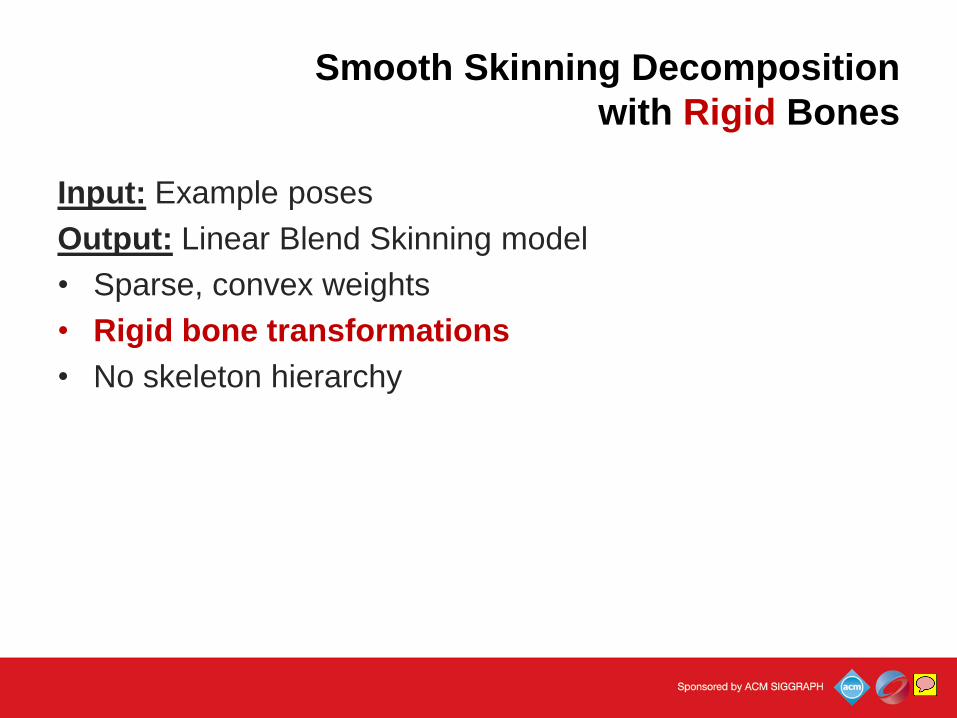
Smooth Skinning Decomposition
with Rigid Bones
Input: Example poses
Output: Linear Blend Skinning model
• Sparse, convex weights
• Rigid bone transformations
• No skeleton hierarchy
BinhLe
Sticky Note
And here is what our model does. From example poses, it generates Linear Blend Skinning model, which consists of a sparse and convex weight map, and rigid bone transformations. Also note that we don’t consider the skeleton hierarchy in this work.
Smooth Skinning Decomposition
with Rigid Bones
Input: Example poses
Output: Linear Blend Skinning model
• Sparse, convex weights
• Rigid bone transformations
• No skeleton hierarchy
Goals:
Approximate highly deformation models
Fast performance
Simple implementation
BinhLe
Sticky Note
Our skinning decomposition model aims for 3 goals: Accurate, fast, and simple.
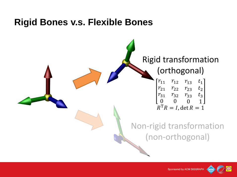
Rigid Bones v.s. Flexible Bones
Rigid transformation (orthogonal)
Non-rigid transformation (non-orthogonal)
𝑟11 𝑟12𝑟21 𝑟22
𝑟13 𝑡1𝑟23 𝑡2
𝑟31 𝑟320 0
𝑟33 𝑡30 1
𝑅T𝑅 = 𝐼, det 𝑅 = 1
BinhLe
Sticky Note
I just mentioned about rigid bone, so why we focus on that? Rigid bone refers to the bone where its transformation matrix is orthogonal and it only includes rotation and translation.
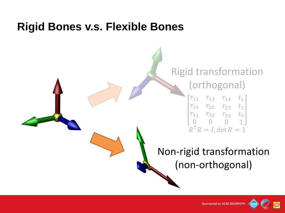
Rigid Bones v.s. Flexible Bones
Rigid transformation (orthogonal)
Non-rigid transformation (non-orthogonal)
𝑟11 𝑟12𝑟21 𝑟22
𝑟13 𝑡1𝑟23 𝑡2
𝑟31 𝑟320 0
𝑟33 𝑡30 1
𝑅T𝑅 = 𝐼, det 𝑅 = 1
BinhLe
Sticky Note
I contrast, we have the flexible bone where the transformation is non-rigid and it also includes scaling and shearing.
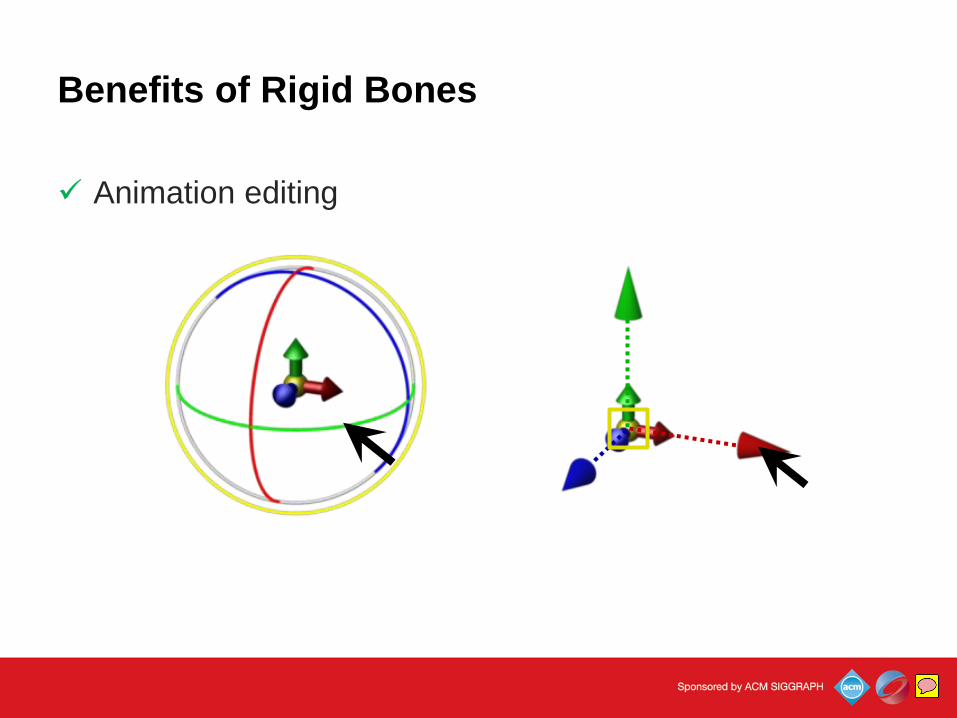
Benefits of Rigid Bones
Animation editing
BinhLe
Sticky Note
And rigid bones can benefit some tasks like animation editing, where the interfaces to control rotation and translation are more intuitive than scaling and shearing.
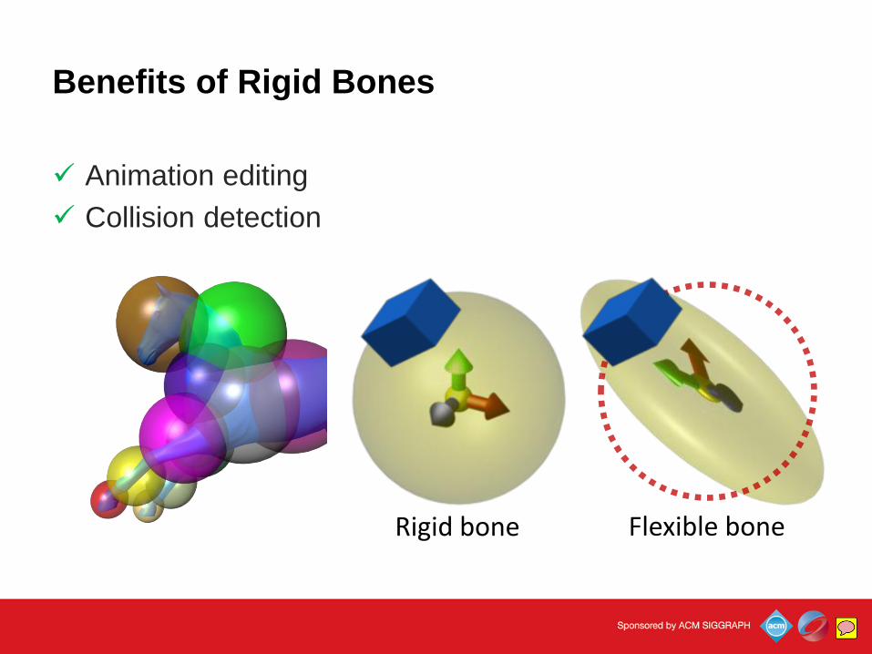
Benefits of Rigid Bones
Animation editing
Collision detection
Rigid bone Flexible bone
BinhLe
Sticky Note
Rigid bones also make the collision detection task easier if the sphere is not distorted by a non-rigid transformation.
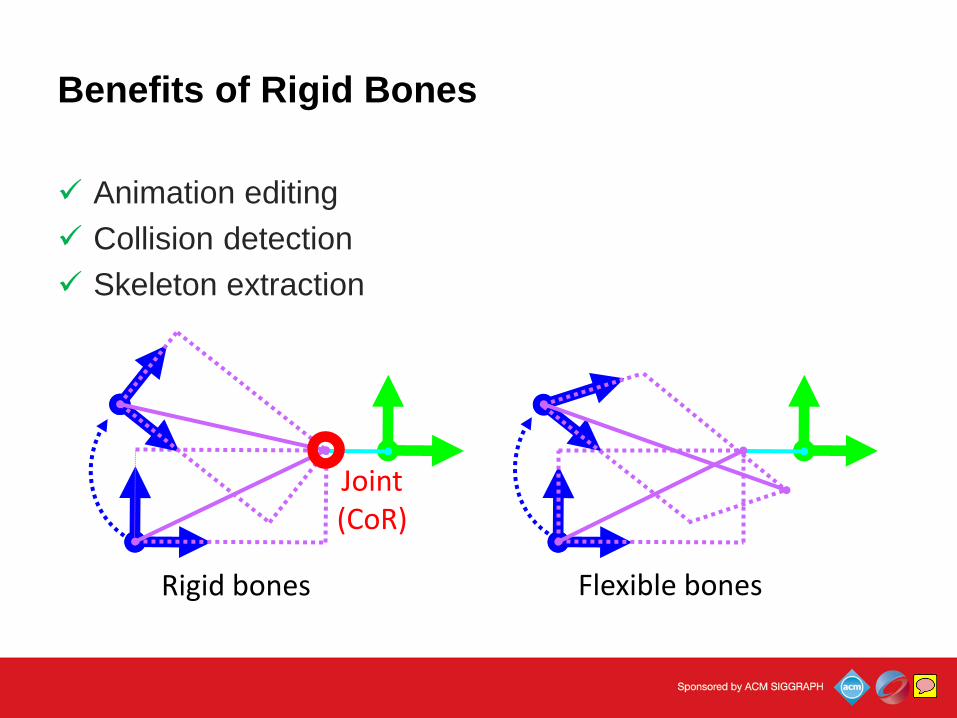
Benefits of Rigid Bones
Animation editing
Collision detection
Skeleton extraction
Joint (CoR)
Rigid bones Flexible bones
BinhLe
Sticky Note
If the two rigid bones have a common center of rotation, they are linked by a joint.
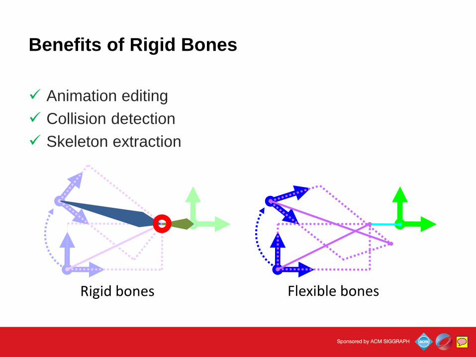
Benefits of Rigid Bones
Animation editing
Collision detection
Skeleton extraction
Flexible bones Rigid bones
BinhLe
Sticky Note
And we can use that to extract the skeleton. However with the flexible bones, we simple have no rotation, and no joint neither.
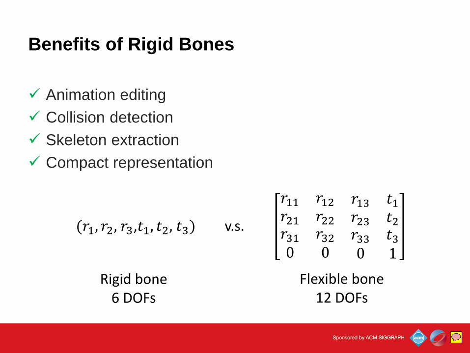
Benefits of Rigid Bones
Animation editing
Collision detection
Skeleton extraction
Compact representation
𝑟11 𝑟12𝑟21 𝑟22
𝑟13 𝑡1𝑟23 𝑡2
𝑟31 𝑟320 0
𝑟33 𝑡30 1
(𝑟1, 𝑟2, 𝑟3,𝑡1, 𝑡2, 𝑡3) v.s.
Rigid bone 6 DOFs
Flexible bone 12 DOFs
BinhLe
Sticky Note
Rigid transformations are also more compact than non-rigid transformations.
Benefits of Rigid Bones
Animation editing
Collision detection
Skeleton extraction
Compact representation
BinhLe
Sticky Note
And that’s why we focus on rigid bones.
Previous Work
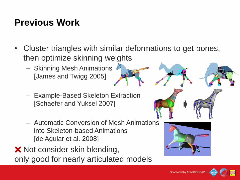
• Cluster triangles with similar deformations to get bones,
then optimize skinning weights
– Skinning Mesh Animations
[James and Twigg 2005]
– Example-Based Skeleton Extraction
[Schaefer and Yuksel 2007]
– Automatic Conversion of Mesh Animations
into Skeleton-based Animations
[de Aguiar et al. 2008]
Not consider skin blending,
only good for nearly articulated models
BinhLe
Sticky Note
There are some previous work on the same problem. One idea is first cluster triangles with similar deformations to get bone transformations, and then solve the skinning weights. Since the clustering does not consider skin blending, it only works well for nearly articulated models.
Previous Work
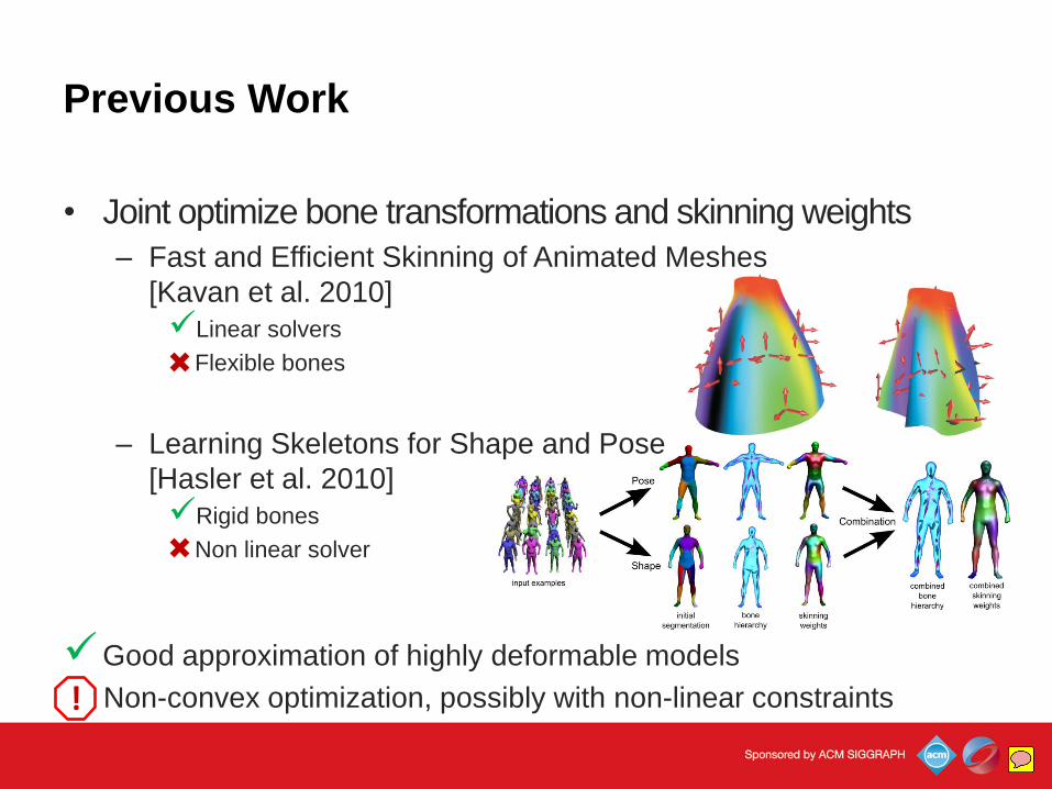
• Joint optimize bone transformations and skinning weights
– Fast and Efficient Skinning of Animated Meshes
[Kavan et al. 2010]
Linear solvers
Flexible bones
– Learning Skeletons for Shape and Pose
[Hasler et al. 2010]
Rigid bones
Non linear solver
Good approximation of highly deformable models
Non-convex optimization, possibly with non-linear constraints !
BinhLe
Sticky Note
Other approach is trying to optimize both bone transformations and skinning weights at the same time. This typically works very well, even with highly deformation model. And in fact, we also do the joint optimization. However the optimization is quite challenge since it is non-convex, possibly comes with non-linear constraints.
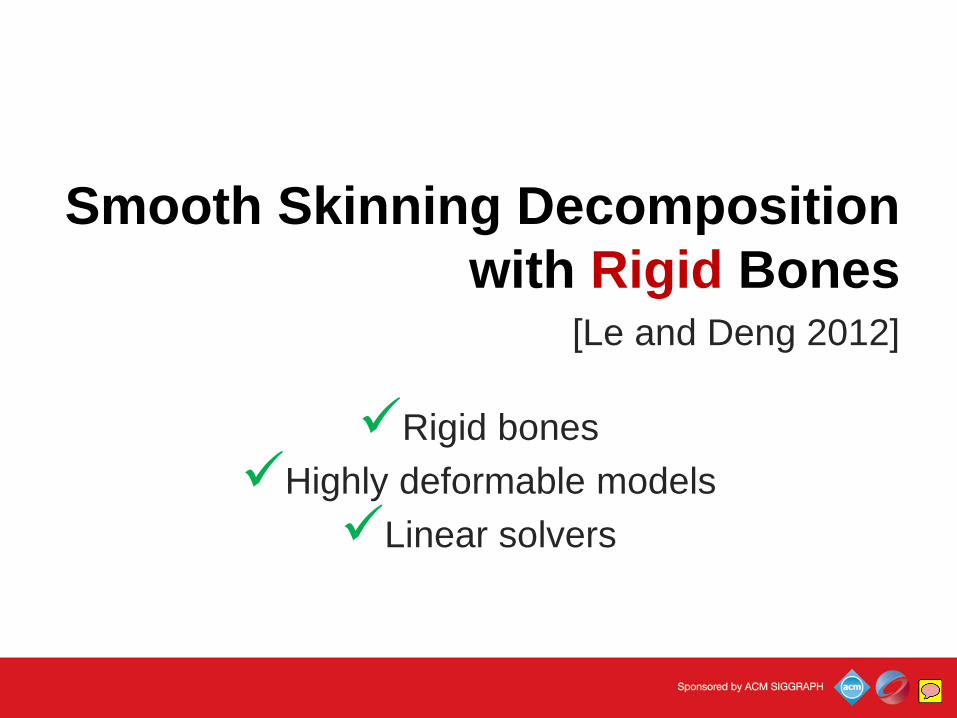
Smooth Skinning Decomposition
with Rigid Bones [Le and Deng 2012]
Rigid bones
Highly deformable models
Linear solvers
BinhLe
Sticky Note
We distinguish our work from previous by focusing on the rigid bones, trying to achieve good approximation even with highly deformable models, and proposing a fast and simple algorithm with all linear solvers.
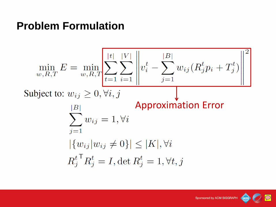
Problem Formulation
Approximation Error
BinhLe
Sticky Note
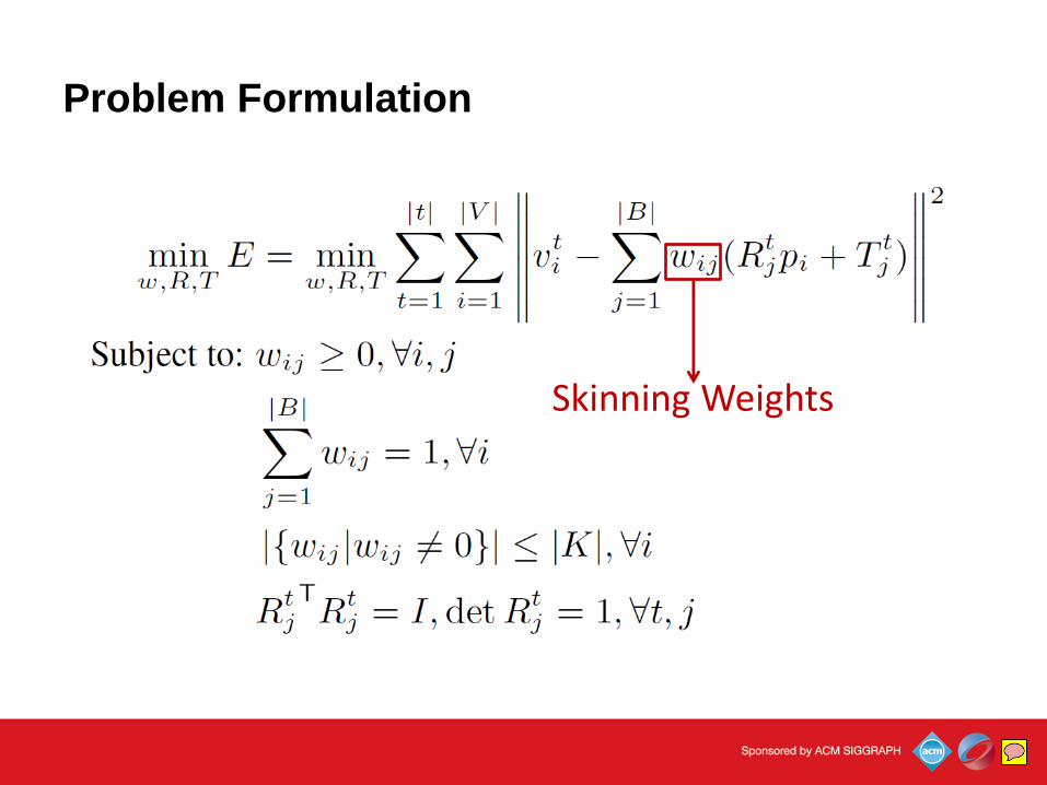
And here is how we formulate our skinning decomposition problem. In this equation, we try to minimize the approximation error for all vertices over all example poses, or basically we need to find a LBS model which best approximate the input…
Problem Formulation
Skinning Weights
BinhLe
Sticky Note
We need to find both the skinning weights…
Problem Formulation
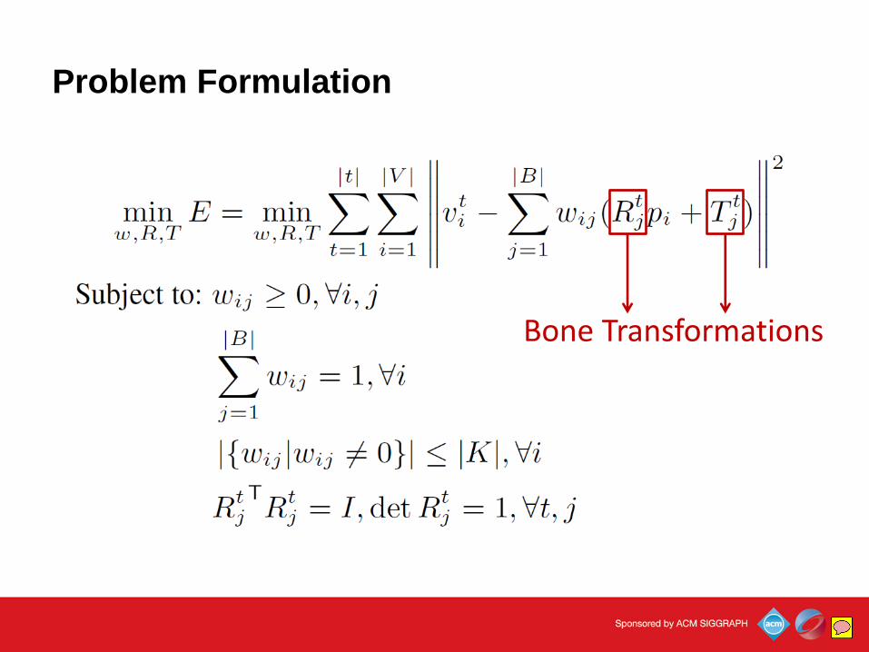
Bone Transformations
BinhLe
Sticky Note
…and the bone transformations…
Problem Formulation
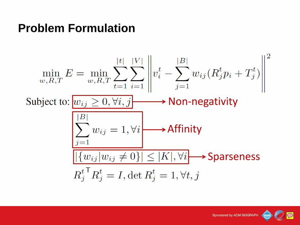
Sparseness
Non-negativity
Affinity
BinhLe
Sticky Note
Recall that we impose several constraints on the skinning model, they are non-negativity, affinity, and sparseness constraint on the weight map.
Problem Formulation
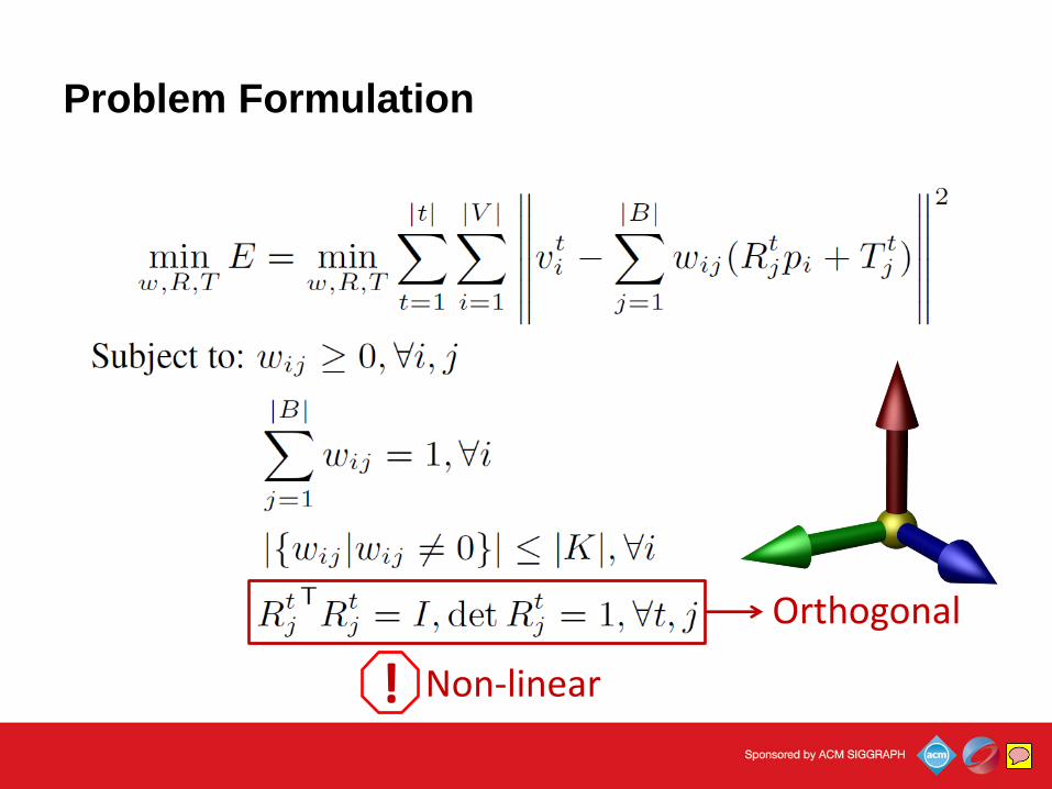
Orthogonal
! Non-linear
BinhLe
Sticky Note
On the bone transformation, we impose the orthogonal constraint. Note that the constraint is a non-linear and it makes the optimization more challenge.
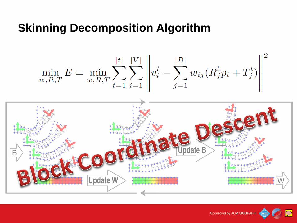
Skinning Decomposition Algorithm
BinhLe
Sticky Note
…and we solve this optimization by a block coordinate descent algorithm…
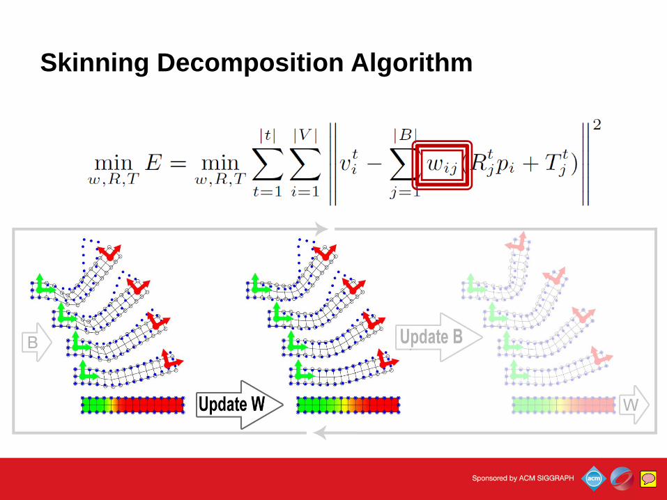
Skinning Decomposition Algorithm
BinhLe
Sticky Note
… where we alternatively update the weight map…
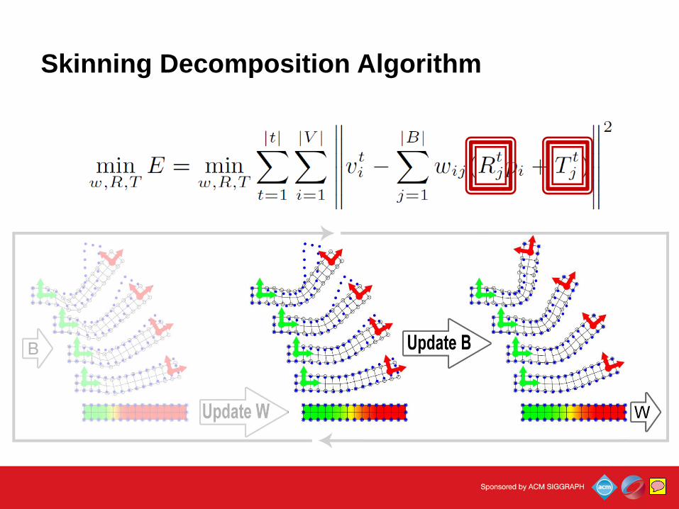
Skinning Decomposition Algorithm
BinhLe
Sticky Note
…and the bone transformation to reduce the approximation error.
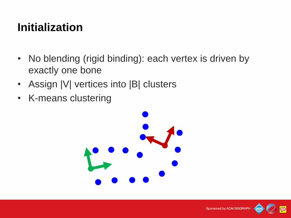
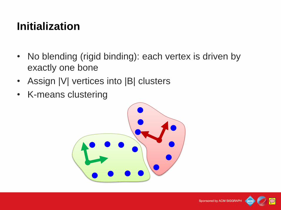
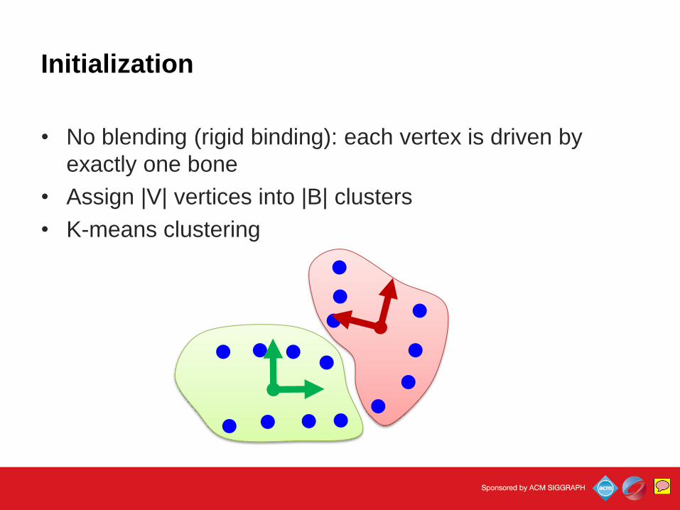
Initialization
• No blending (rigid binding): each vertex is driven by
exactly one bone
• Assign |V| vertices into |B| clusters
• K-means clustering
BinhLe
Sticky Note
But first we need to initialize a feasible solution, in this step we assume no blending on the model so that the deformation is as rigid as possible. In other words, we have a rigid bind where each vertex is driven b exactly one bone. Our initialization then become a clustering problem and we just do a K-means clustering.
Initialization
• No blending (rigid binding): each vertex is driven by
exactly one bone
• Assign |V| vertices into |B| clusters
• K-means clustering
BinhLe
Sticky Note
We alternatively assign each vertex to the bone with lowest reconstruction error…
Initialization
• No blending (rigid binding): each vertex is driven by
exactly one bone
• Assign |V| vertices into |B| clusters
• K-means clustering
BinhLe
Sticky Note
…and update the bone by finding the best rigid transformation of the vertex set. Note that this is a simple version of our main algorithm where we don’t consider skin blending. And you can always choose more robust but slower clustering algorithms.
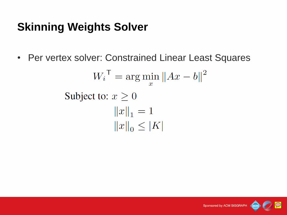
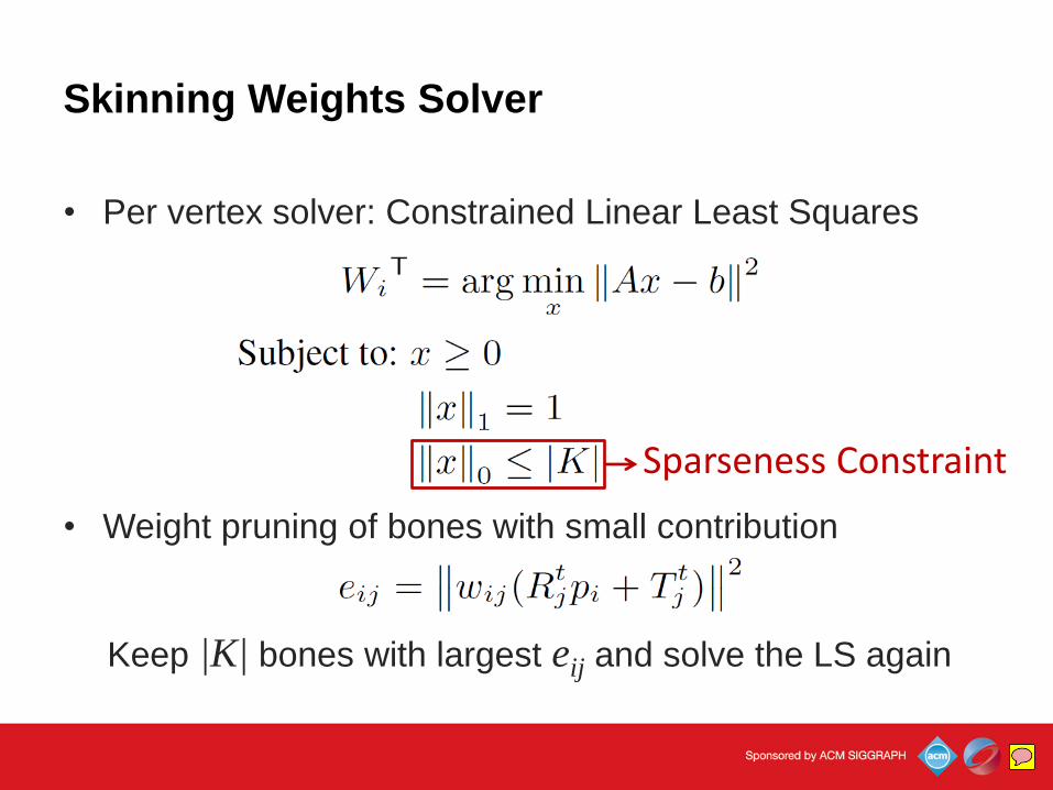
Skinning Weights Solver
• Per vertex solver: Constrained Linear Least Squares
BinhLe
Sticky Note
After initialization, we solve for the skinning weights. This is a constrained linear least squares.
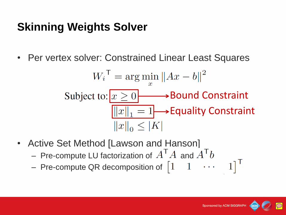
Skinning Weights Solver
• Per vertex solver: Constrained Linear Least Squares
• Active Set Method [Lawson and Hanson]
– Pre-compute LU factorization of and
– Pre-compute QR decomposition of
Bound Constraint
Equality Constraint
BinhLe
Sticky Note
And we handle the bound constraint and the equality constraint with the Active Set Method. To accelerate the process, we pre-compute the LU factorization of these cross products, and the QR decomposition of the unit vectors with all 1 numbers.
Skinning Weights Solver
• Per vertex solver: Constrained Linear Least Squares
• Weight pruning of bones with small contribution
Sparseness Constraint
Keep |K| bones with largest eij and solve the LS again
BinhLe
Sticky Note
To handle the sparseness constraint, we prune bones with small contribution to the deformation and solve the least squares again with K remaining bones.
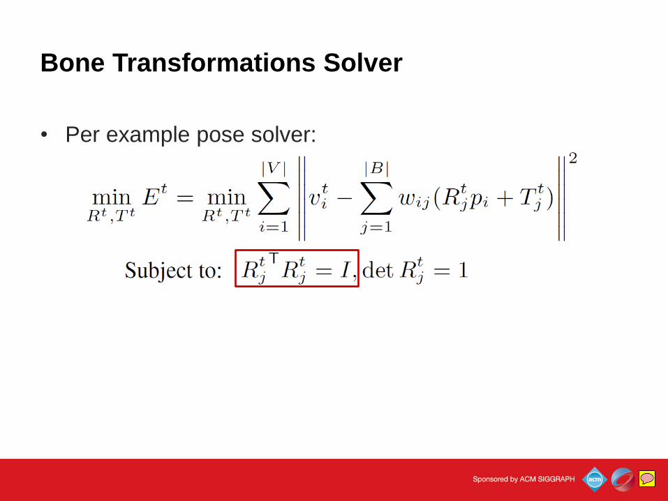
Bone Transformations Solver
• Per example pose solver:
BinhLe
Sticky Note
Previous are easy parts, and now we come to the hard one, updating the bone transformation with non-rigid constraints.
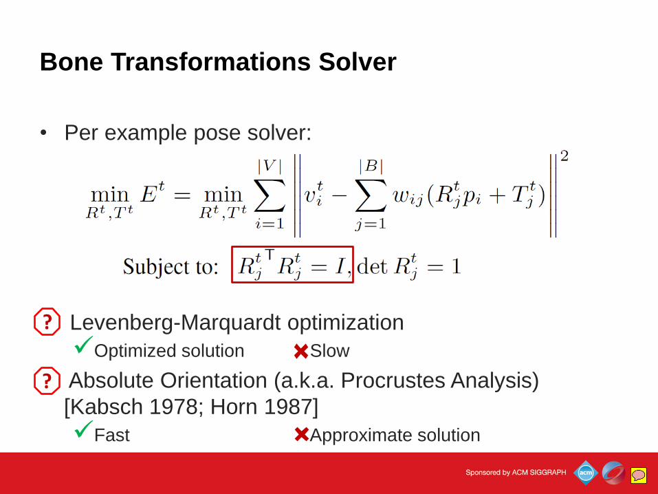
Bone Transformations Solver
• Per example pose solver:
Levenberg-Marquardt optimization
Optimized solution Slow
Absolute Orientation (a.k.a. Procrustes Analysis)
[Kabsch 1978; Horn 1987]
Fast Approximate solution
?
?
BinhLe
Sticky Note
There are two common solutions for this problem: Using the non-linear Levenberg-Marquardt optimization, or using the Absolute Orientation solution also known as Procrustes Analysis. And both methods have advantages and disadvantages.
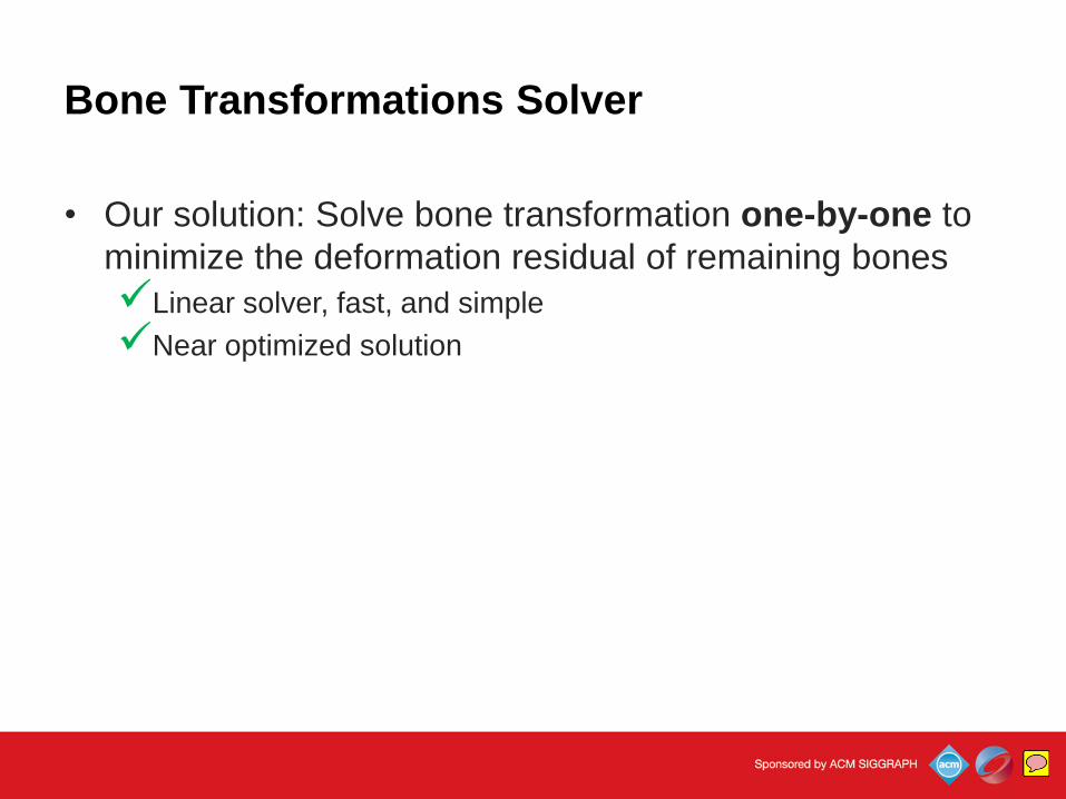
Bone Transformations Solver
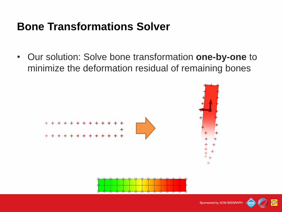
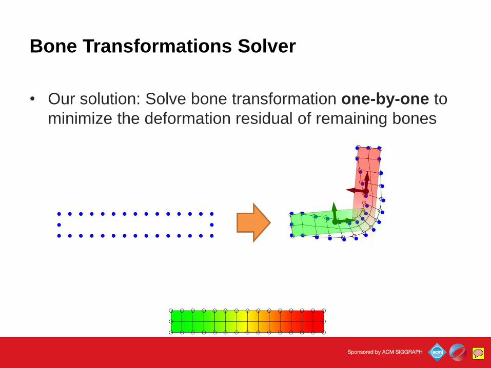
• Our solution: Solve bone transformation one-by-one to
minimize the deformation residual of remaining bones
Linear solver, fast, and simple
Near optimized solution
BinhLe
Sticky Note
Instead of that, we propose a fast linear solution which gives a very good solution. We update the bone transformations one by one while keeping the others fixed. And in each update, we try to minimize the deformation residual of the remaining bones.
Bone Transformations Solver
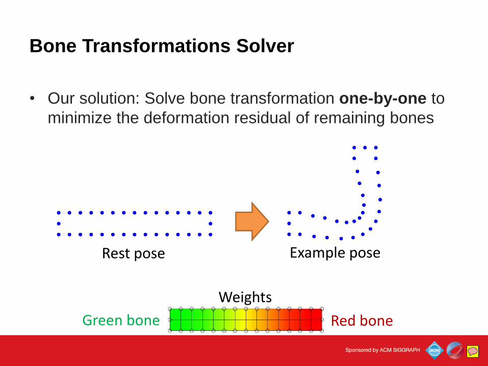
• Our solution: Solve bone transformation one-by-one to
minimize the deformation residual of remaining bones
Rest pose Example pose
Weights
Green bone Red bone
BinhLe
Sticky Note
Let’s take a toy example where we need to find the two bone transformations to deform the rest pose on the left to the example pose on the right, given the current skinning weights on the bottom.
Bone Transformations Solver
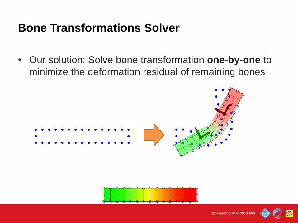
• Our solution: Solve bone transformation one-by-one to
minimize the deformation residual of remaining bones
BinhLe
Sticky Note
Suppose we start with the current bone transformations like this.
Bone Transformations Solver
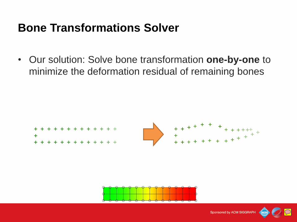
• Our solution: Solve bone transformation one-by-one to
minimize the deformation residual of remaining bones
BinhLe
Sticky Note
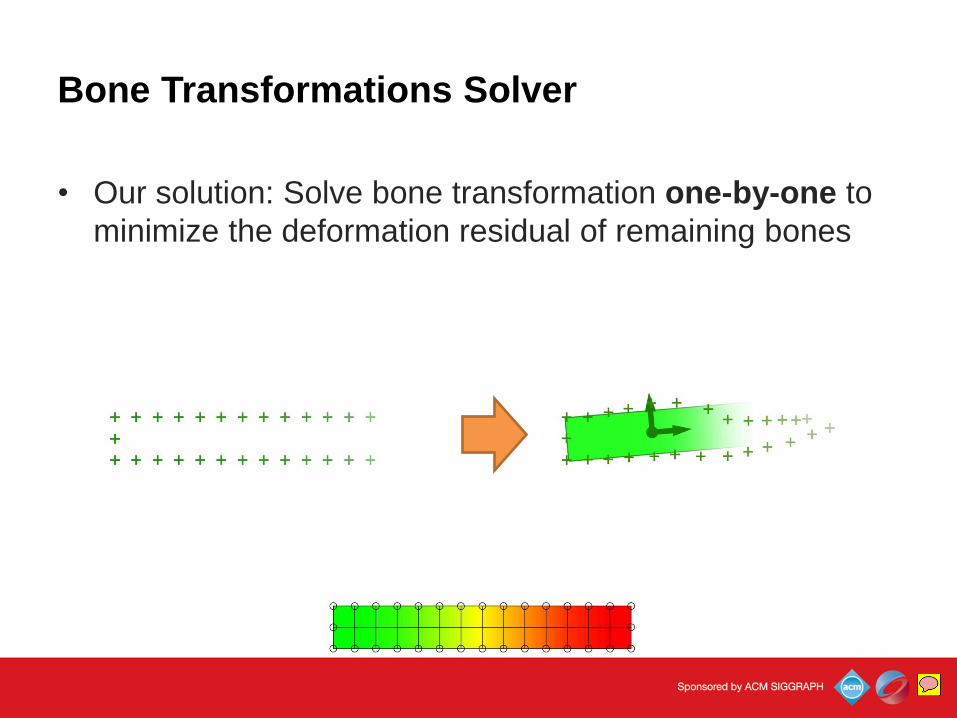
We first calculate the deformation residual for the green bone.
Bone Transformations Solver
• Our solution: Solve bone transformation one-by-one to
minimize the deformation residual of remaining bones
BinhLe
Sticky Note
And fit the rigid transformation to it.
Bone Transformations Solver
• Our solution: Solve bone transformation one-by-one to
minimize the deformation residual of remaining bones
BinhLe
Sticky Note
Then we repeat the same thing with the red bone.
Bone Transformations Solver
• Our solution: Solve bone transformation one-by-one to
minimize the deformation residual of remaining bones
BinhLe
Sticky Note
And finally this is the bone transformations we have.
Bone Transformations Solver
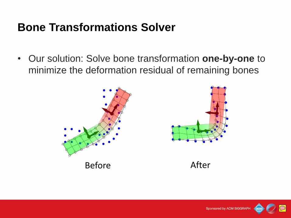
• Our solution: Solve bone transformation one-by-one to
minimize the deformation residual of remaining bones
Before After
BinhLe
Sticky Note
Here are the bone transformations before and after update.
Bone Transformations Solver
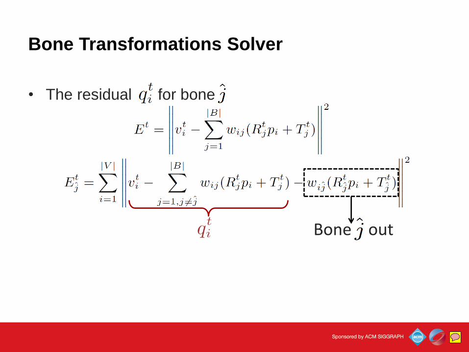
• The residual for bone
Bone out
BinhLe
Sticky Note
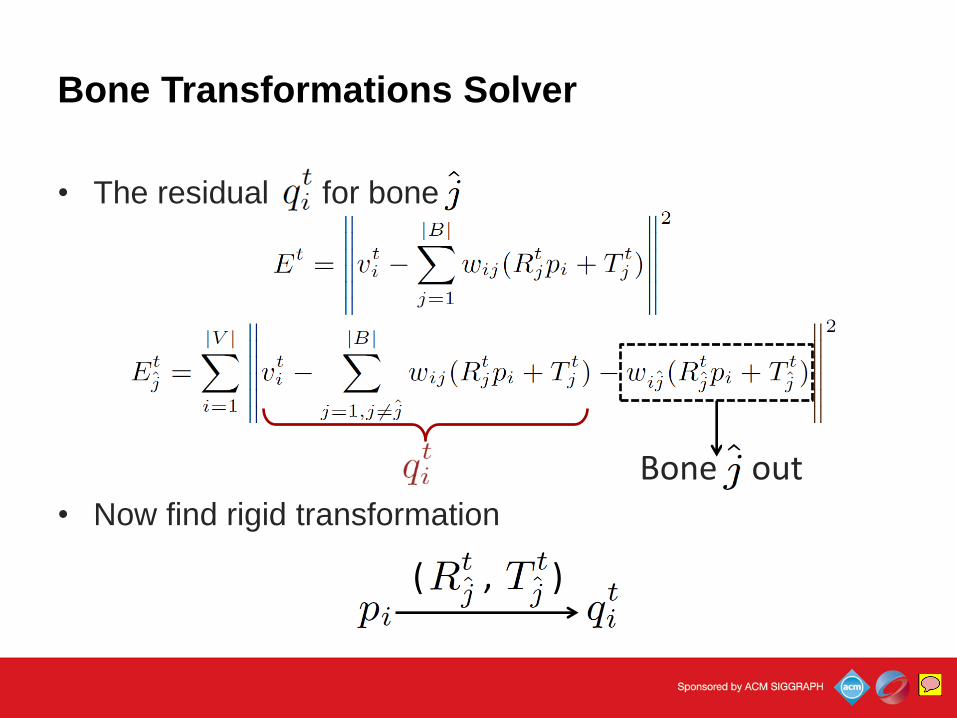
I just mentioned about the deformation residual, so what it is? For a bone j hat, the residual is nothing but the deformation when we keep other bones fixed and discard the j hat bone. And the residual can be considered as a set of vertices correspond to the vertices of our 3D model.
Bone Transformations Solver
• The residual for bone
• Now find rigid transformation
Bone out
( , )
BinhLe
Sticky Note
And now problem becomes finding a rigid transformation to relate two set or vertices.
Bone Transformations Solver
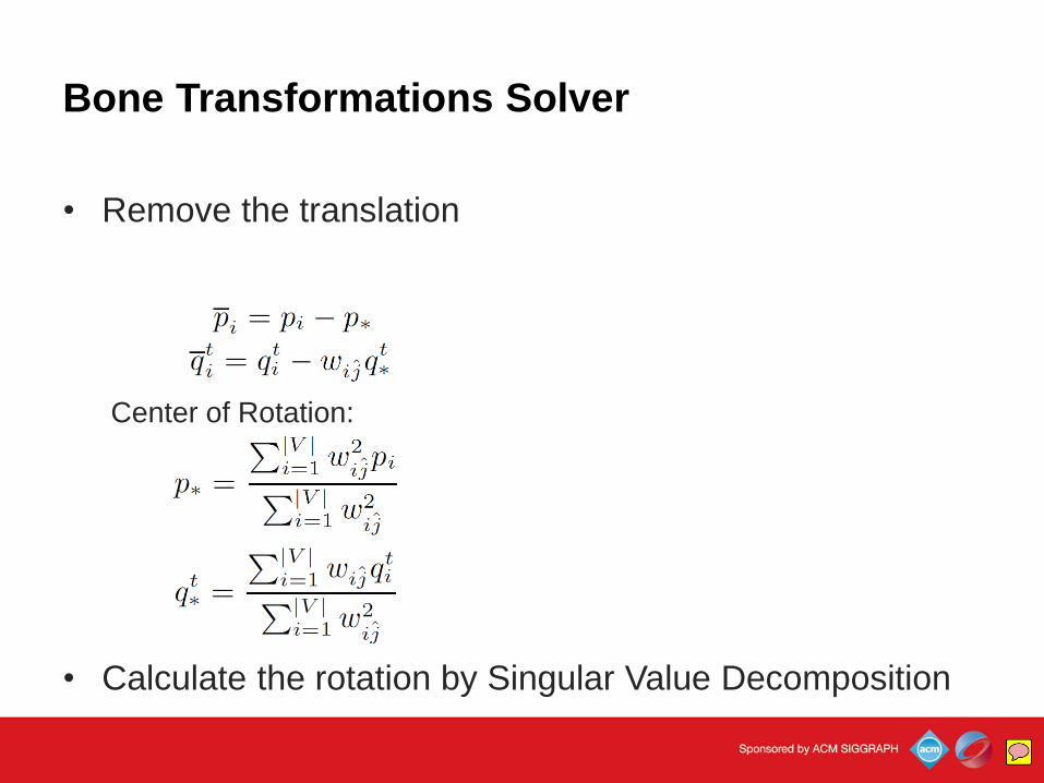
• Remove the translation
Center of Rotation:
• Calculate the rotation by Singular Value Decomposition
BinhLe
Sticky Note
And we solve this problem by a traditional way: first we remove the translation by subtracting each vertex to the center of rotations. And we perform Singular Value Decomposition to get the rotation matrix.
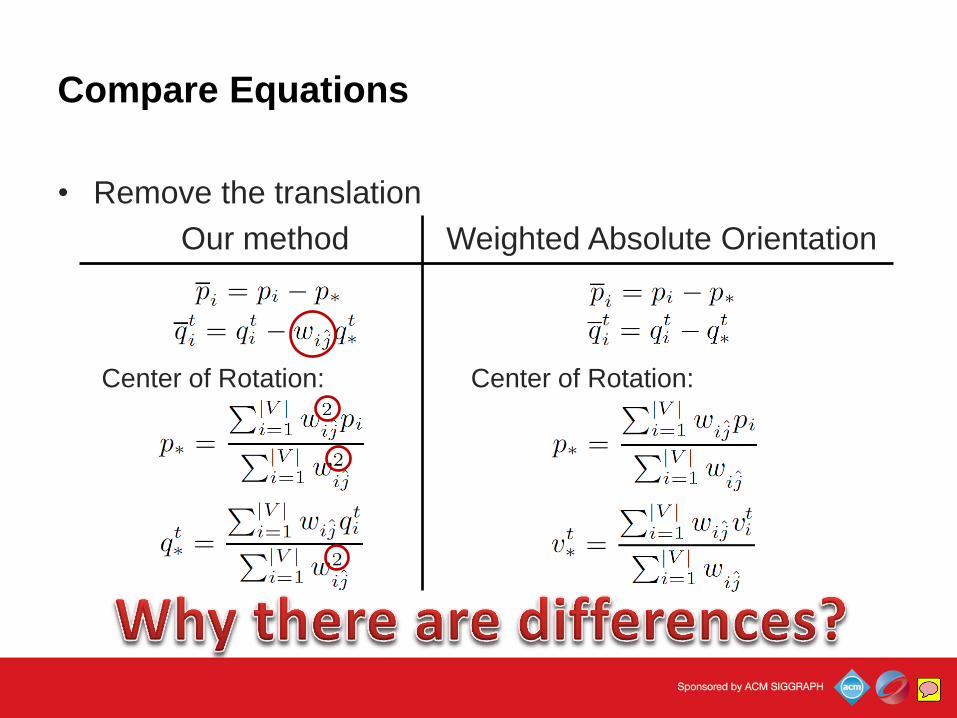
Compare Equations
• Remove the translation
Our method Weighted Absolute Orientation
Center of Rotation: Center of Rotation:
BinhLe
Sticky Note
You can see this is pretty similar to the Absolute Orientation algorithm I mentioned before. However there are some differences on removing the translation part.
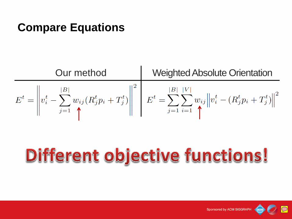
Compare Equations
Our method Weighted Absolute Orientation
BinhLe
Sticky Note
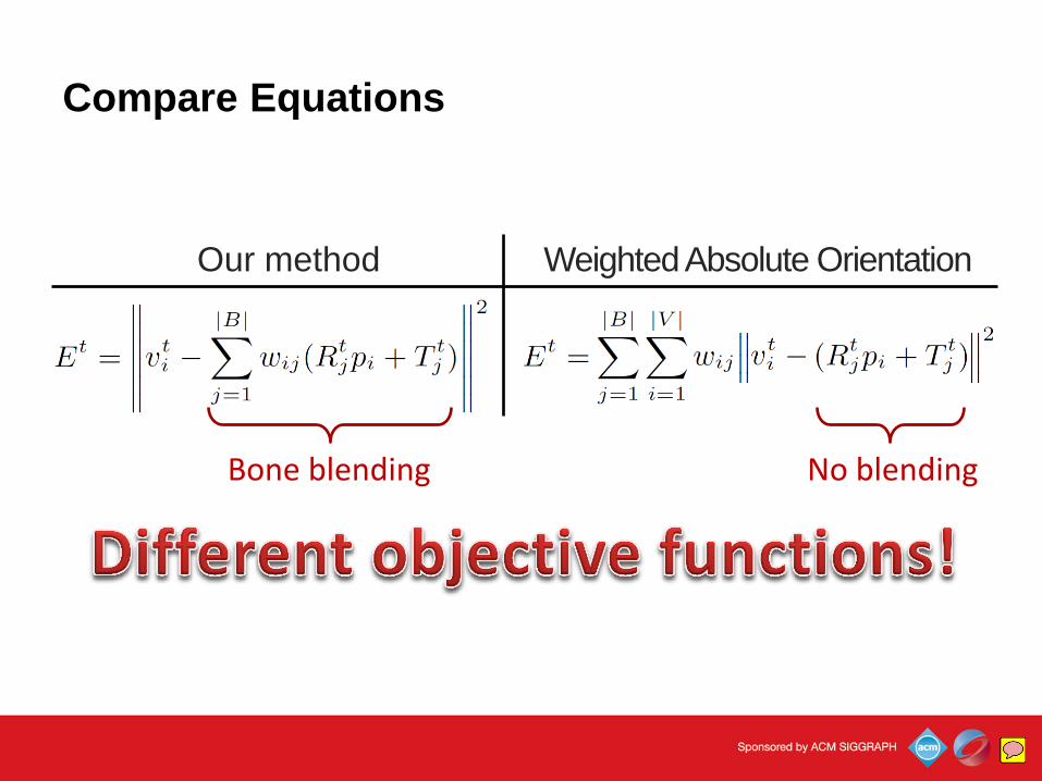
And we have differences because the objective functions are different. Here you can see the scope of the weight terms are different.
Compare Equations
Our method Weighted Absolute Orientation
Bone blending No blending
BinhLe
Sticky Note
And you can see that there is actually no transformation blending in the formulation of Absolute Orientation problem.
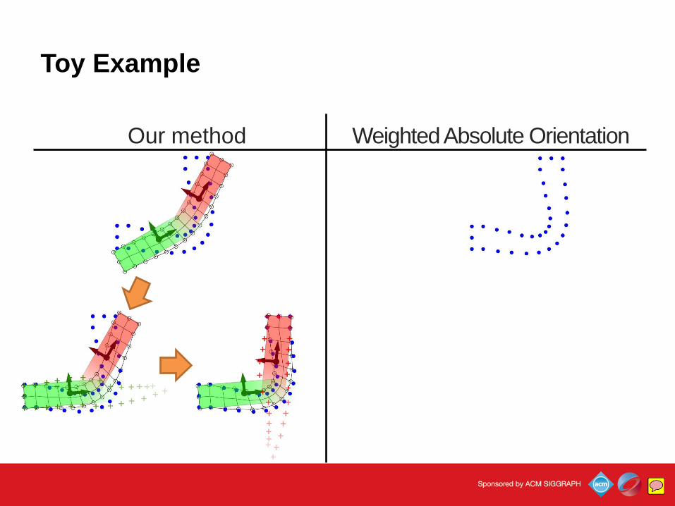
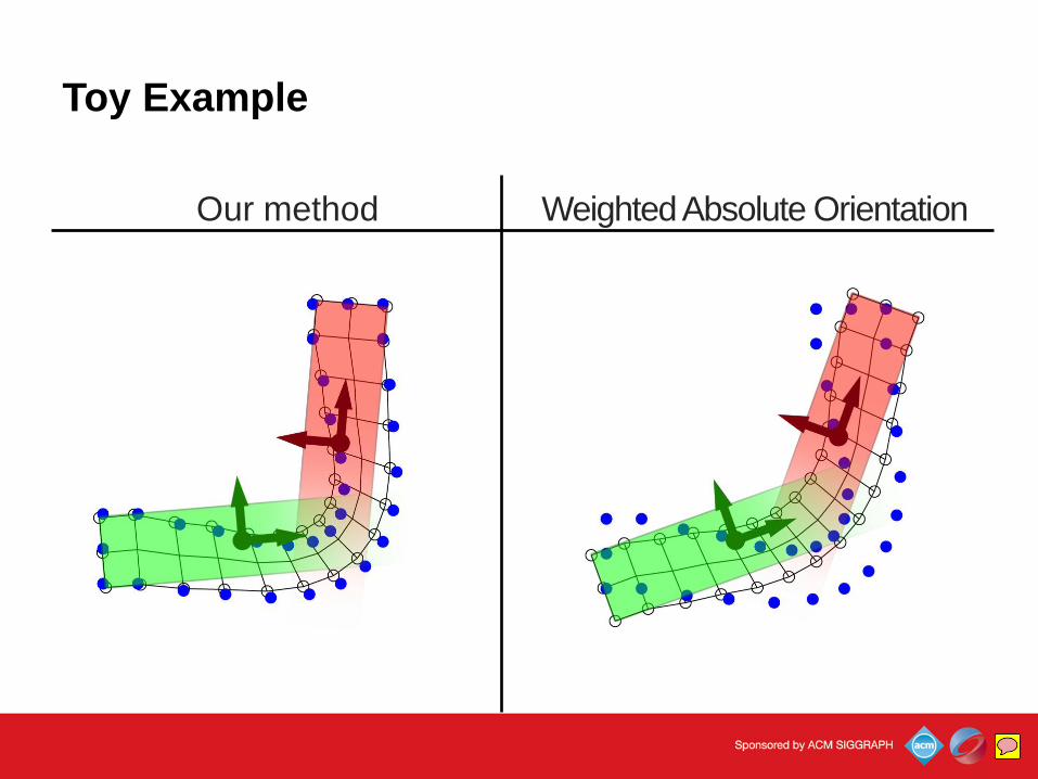
Toy Example
Our method Weighted Absolute Orientation
BinhLe
Sticky Note
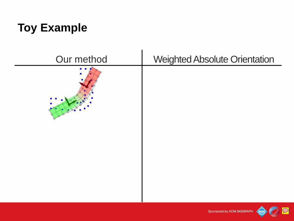
To see how the difference affect to the results, I will show the toy example with two bones again. So we start with this bone transformations and suppose we want to get the deformation close to the blue dots.
Toy Example
Our method Weighted Absolute Orientation
BinhLe
Sticky Note
So first we update the green bone with the residual.
Toy Example
Our method Weighted Absolute Orientation
BinhLe
Sticky Note
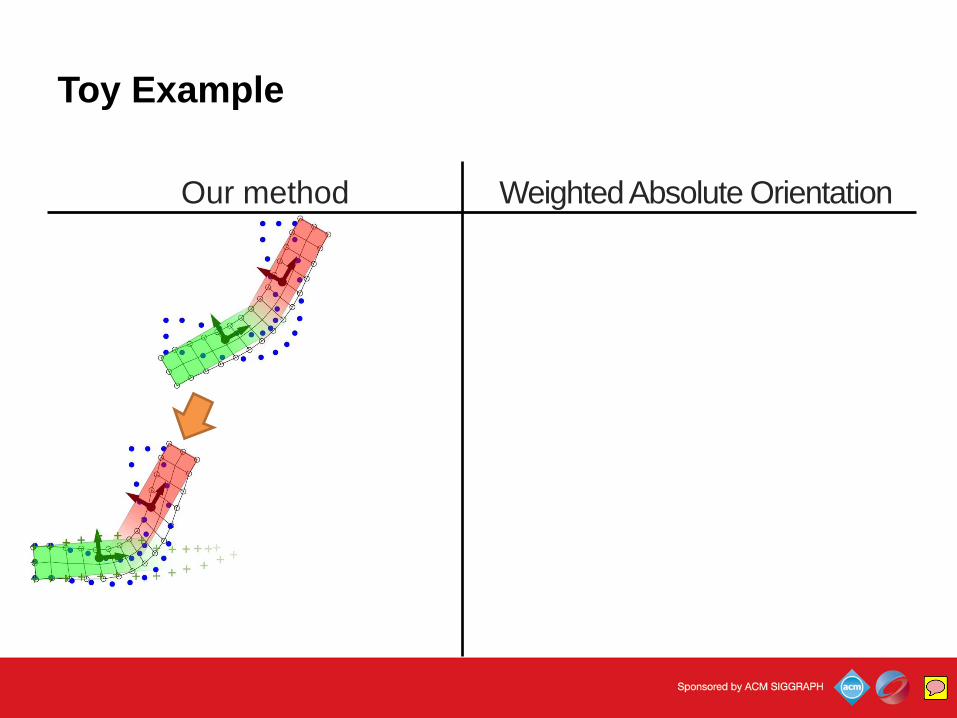
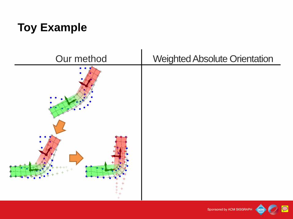
Then we update the red bone and get the final result.
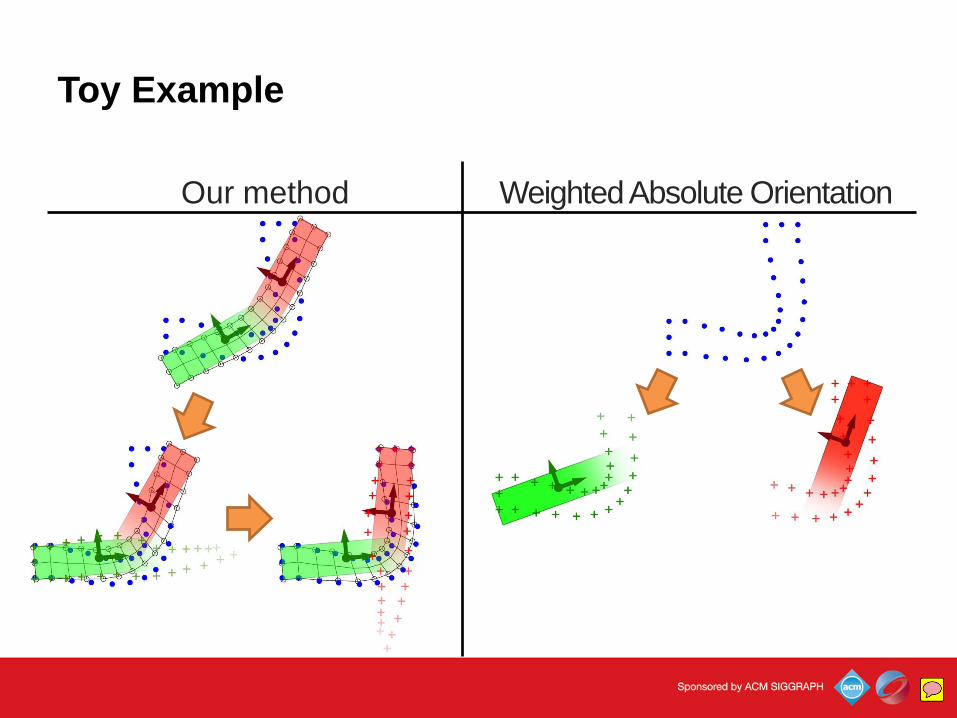
Toy Example
Our method Weighted Absolute Orientation
BinhLe
Sticky Note
For the Absolute Orientation with the same deformation target.
Toy Example
Our method Weighted Absolute Orientation
BinhLe
Sticky Note
It actually solve both transformations at the same time. Note that the green and red plus here are not residuals but just positions on target deformation with weights.
Toy Example
Our method Weighted Absolute Orientation
BinhLe
Sticky Note
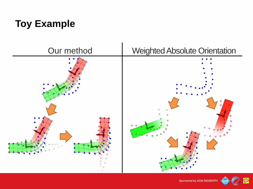
And finally Absolute Orientation gives this.
Toy Example
Our method Weighted Absolute Orientation
BinhLe
Sticky Note
Compare to the Absolute Orientation, the green and red dots in our method are residual. And you can see they are some what more rigid, which means they are easier to fit with the rigid transformations.
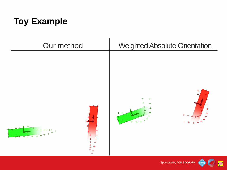
Toy Example
Our method Weighted Absolute Orientation
BinhLe
Sticky Note
And here is the side-by side comparison of the results. You can see our method has better approximation.
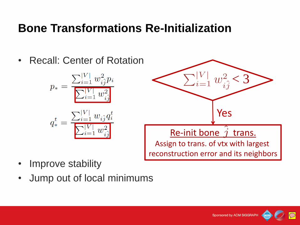
Bone Transformations Re-Initialization
• Recall: Center of Rotation
• Improve stability
• Jump out of local minimums
< 3
Re-init bone trans. Assign to trans. of vtx with largest
reconstruction error and its neighbors
Yes
BinhLe
Sticky Note
Our algorithm some time need to re-initialize the bone transformation. Recalling how we compute the center of rotation to remove the translation. Sometime the denominator here is small, in that case, the influence of the bone is small, and we are wasting it. So we just discard it, and assign it to another place, in this case we just choose the place with worse approximation. This initialization help to improve stability and it somewhat helps to jump out of local minimums.
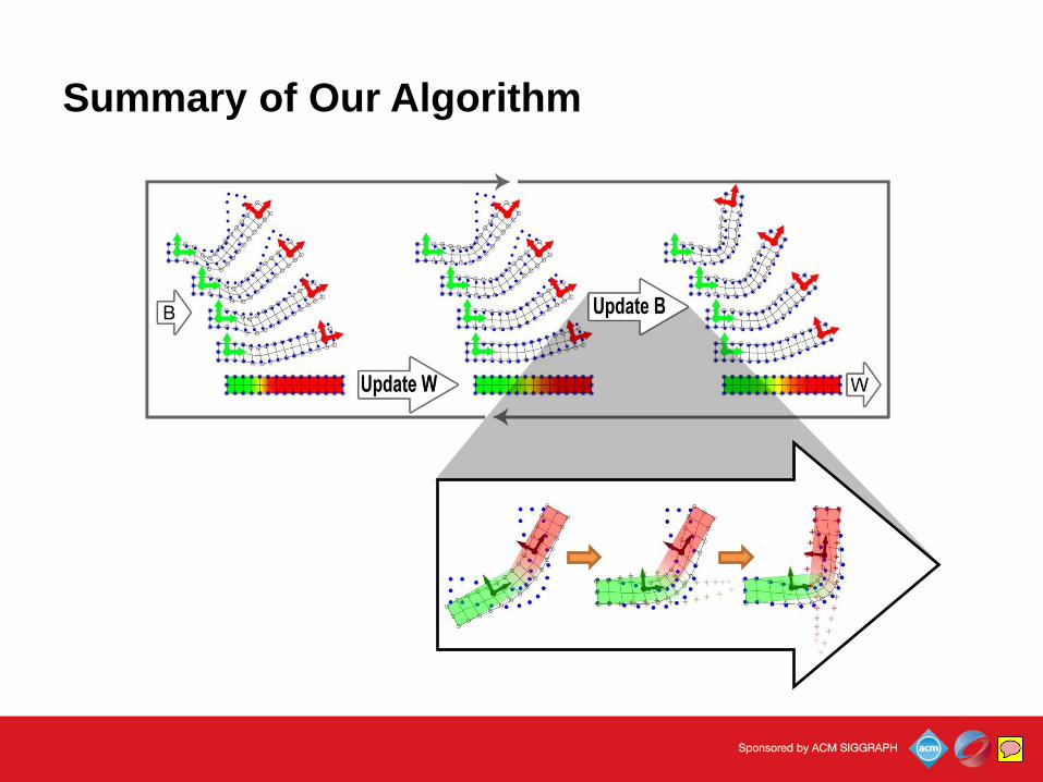
Summary of Our Algorithm
BinhLe
Sticky Note
Putting everything together, I can summarize our algorithm here. It is a block coordinate descent with a loop of updating weights and updating bone transformations. And in the bone transformations update step, we update the bone one by one while keeping other fixed.
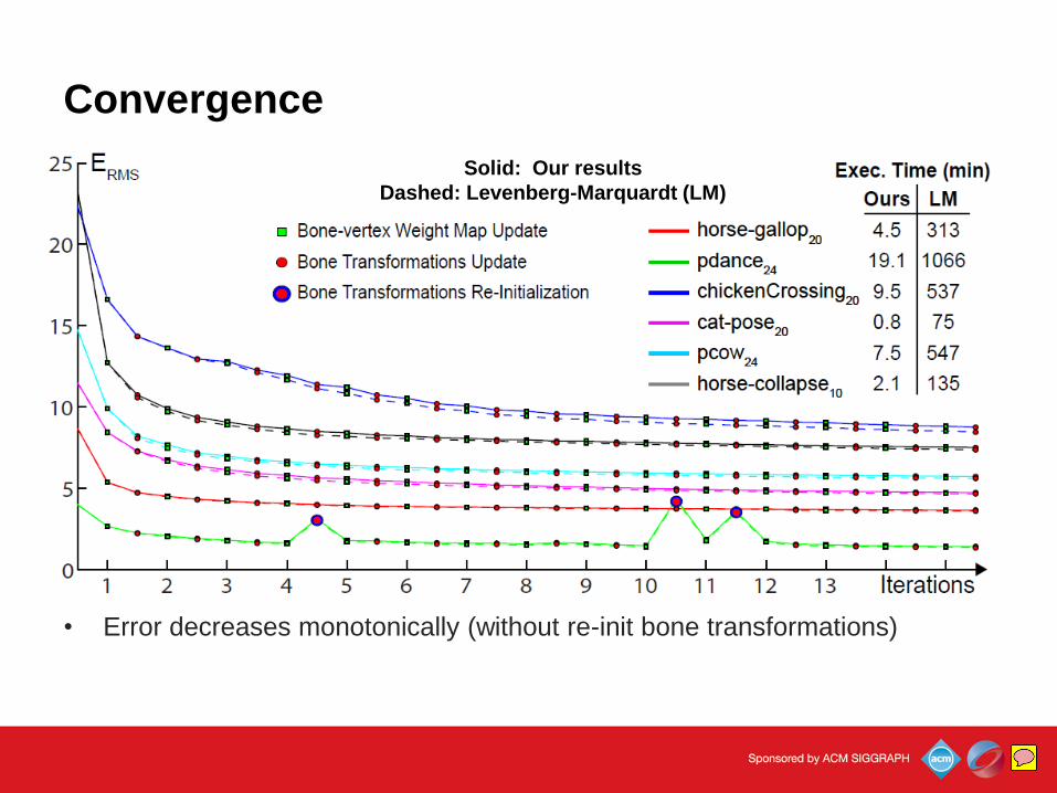
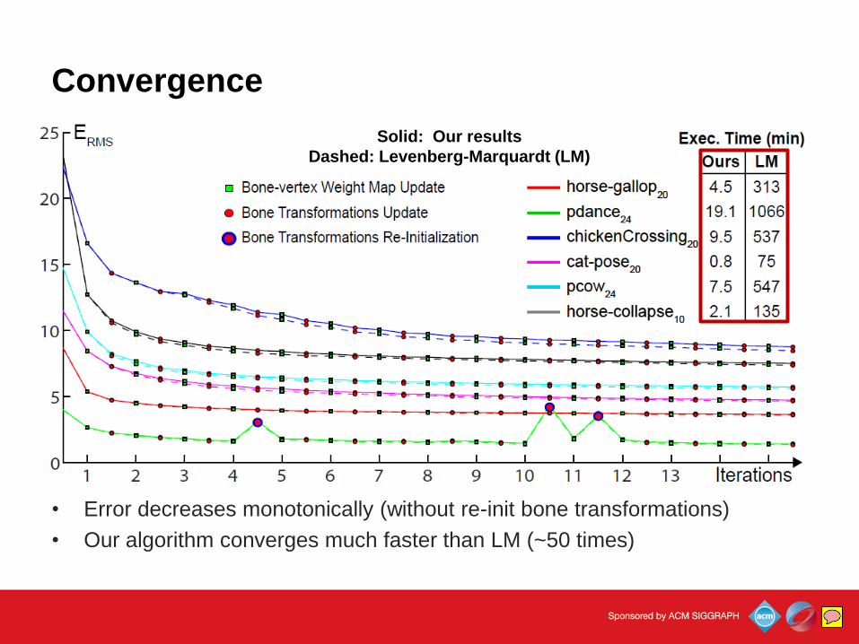
Convergence
• Error decreases monotonically (without re-init bone transformations)
Solid: Our results
Dashed: Levenberg-Marquardt (LM)
BinhLe
Sticky Note
Here I show how the approximation error converge after each update. We can see our method strictly converge without bone transformation re-initialization. However the re-initialization is controllable and instead of reusing the bone, you can just discard it or you can limit the number of initialization. So it would not be an issue with convergence.
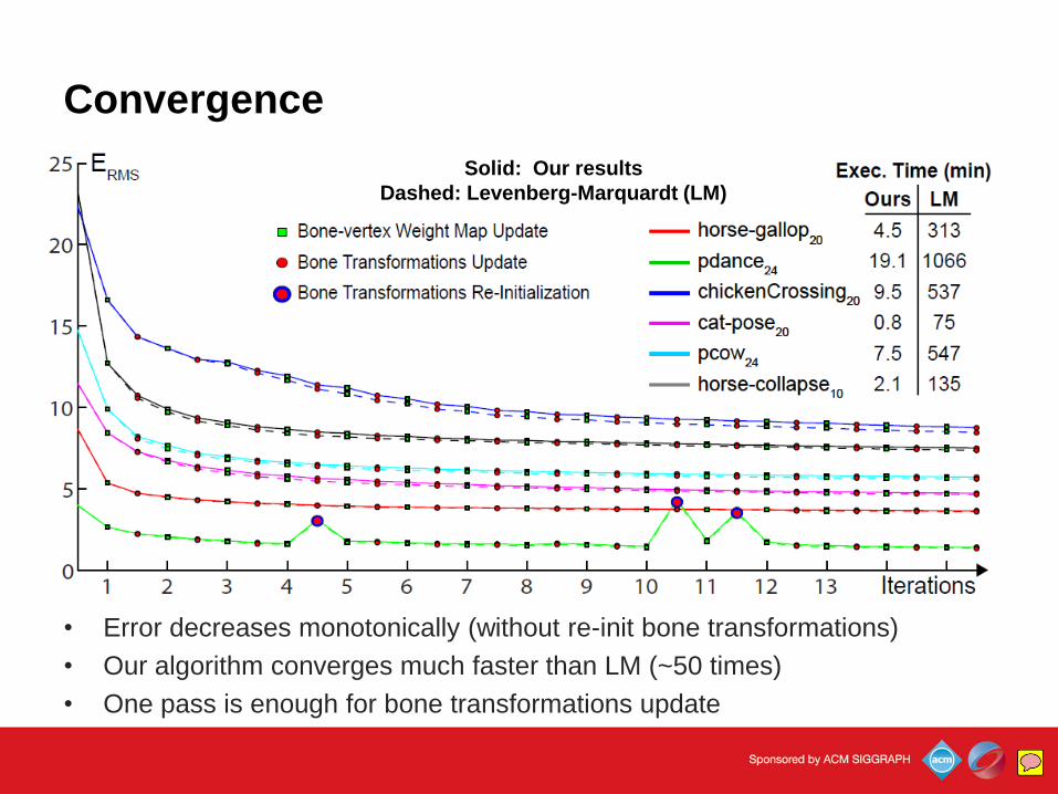
Convergence
• Error decreases monotonically (without re-init bone transformations)
• Our algorithm converges much faster than LM (~50 times)
Solid: Our results
Dashed: Levenberg-Marquardt (LM)
BinhLe
Sticky Note
Compare to the LM optimization, we achieve much better convergence rate since the error drops almost the same while our execution time is much faster. If you look at the table on the right hand side, you can see our method is about 50 times faster.
Convergence
• Error decreases monotonically (without re-init bone transformations)
• Our algorithm converges much faster than LM (~50 times)
• One pass is enough for bone transformations update
Solid: Our results
Dashed: Levenberg-Marquardt (LM)
BinhLe
Sticky Note
And finally, this result shows that one pass bone transformation update is enough to bring the result close to the optimum. But in other cases, if you need to solve the bone transformations alone without alternating update the weights, you’d better repeat the bone transformation updates more than once.
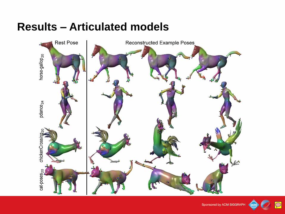
Results – Articulated models
BinhLe
Sticky Note
And here are some skinning decomposition results with articulated models.
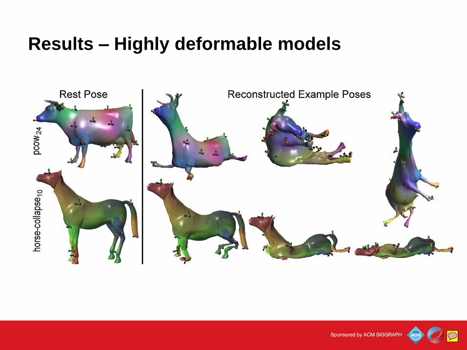
Results – Highly deformable models
BinhLe
Sticky Note
And next are results with highly deformable models. You can see here we use rigid transformation to approximate highly non-rigid models. But how good it is?
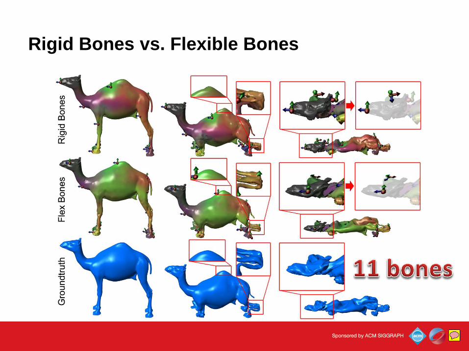
Rigid Bones vs. Flexible Bones
BinhLe
Sticky Note
So we do the comparison between rigid and flexible bones. As you can see, on the top row, 11 rigid bones can approximate the collapsing camel quite well. Although the detail deformations are not as good as the using flexible bones, but the global deformations are ok.
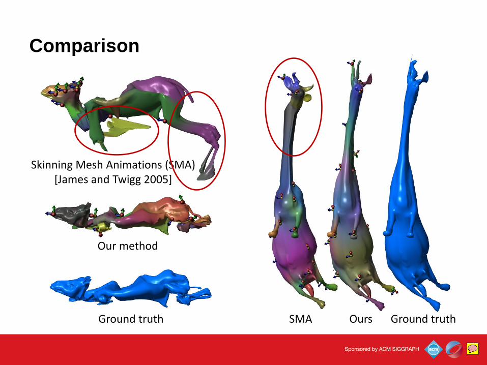
Comparison
Our method
Ground truth SMA Ours Ground truth
Skinning Mesh Animations (SMA) [James and Twigg 2005]
BinhLe
Sticky Note
We also did comparisons with previous method. Here the differences are quite clear. It is because our alternative updating works much better than the one-shot solution of clustering bone transformations, then solving the weights.
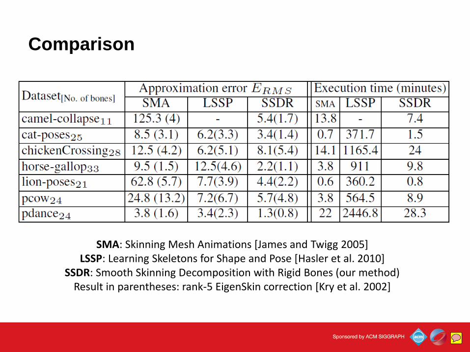
Comparison
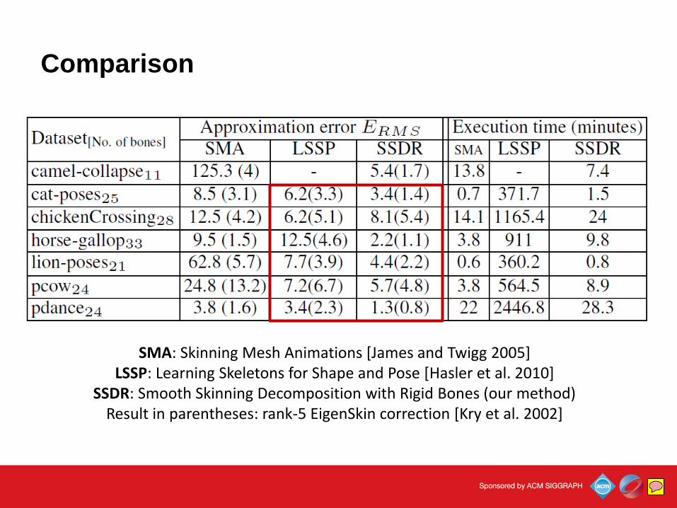
SMA: Skinning Mesh Animations [James and Twigg 2005] LSSP: Learning Skeletons for Shape and Pose [Hasler et al. 2010]
SSDR: Smooth Skinning Decomposition with Rigid Bones (our method) Result in parentheses: rank-5 EigenSkin correction [Kry et al. 2002]
BinhLe
Sticky Note
This table show the comparison in the quantitative way with approximation errors.
Comparison
SMA: Skinning Mesh Animations [James and Twigg 2005] LSSP: Learning Skeletons for Shape and Pose [Hasler et al. 2010]
SSDR: Smooth Skinning Decomposition with Rigid Bones (our method) Result in parentheses: rank-5 EigenSkin correction [Kry et al. 2002]
BinhLe
Sticky Note
Again you can see clear differences with one-shot clustering solution.
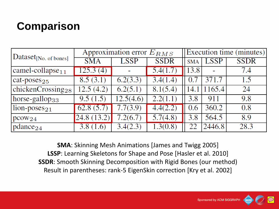
Comparison
SMA: Skinning Mesh Animations [James and Twigg 2005] LSSP: Learning Skeletons for Shape and Pose [Hasler et al. 2010]
SSDR: Smooth Skinning Decomposition with Rigid Bones (our method) Result in parentheses: rank-5 EigenSkin correction [Kry et al. 2002]
BinhLe
Sticky Note
And see slightly differences with other alternative updating method.
Comparison
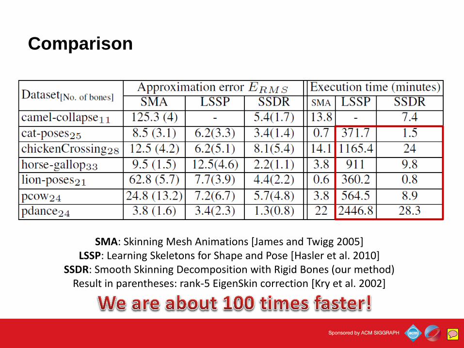
SMA: Skinning Mesh Animations [James and Twigg 2005] LSSP: Learning Skeletons for Shape and Pose [Hasler et al. 2010]
SSDR: Smooth Skinning Decomposition with Rigid Bones (our method) Result in parentheses: rank-5 EigenSkin correction [Kry et al. 2002]
BinhLe
Sticky Note
However, we can see a big gap in performance here since the Learning Skeletons for Shape and Pose employs the LM.
Conclusion
Linear Blend Skinning Decomposition Model
• Convex, sparse weights
Rigid bone transformations
Iterative bone transformation linear solvers
Nearly optimized, working well with highly deformation models
Fast
Simple
BinhLe
Sticky Note
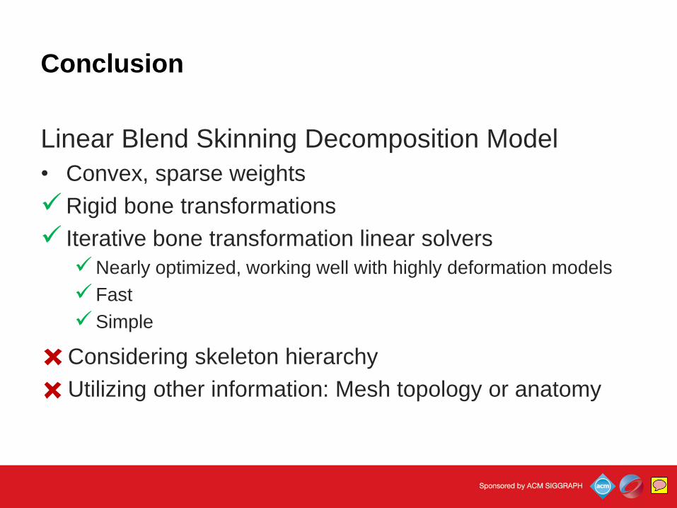
So, in conclusion, I have introduced a linear blend skinning decomposition model. Our model supports convex and sparseness constraints on the skinning weights. And our main contribution is solving the rigid bone transformation with effective linear solvers.
Conclusion
Linear Blend Skinning Decomposition Model
• Convex, sparse weights
Rigid bone transformations
Iterative bone transformation linear solvers
Nearly optimized, working well with highly deformation models
Fast
Simple
Considering skeleton hierarchy
Utilizing other information: Mesh topology or anatomy
BinhLe
Sticky Note
However, this work still has some limitations which we want to address in the future, they are considering the skeleton hierarchy and utilizing other information such as mesh topology or model anatomy.
Acknowledgements
• NSF IIS-0915965
• Vietnam Education Foundation (VEF)
• Google and Nokia for research gifts
• Robert Sumner, Jovan Popovic, Hugues Hoppe, Doug James, and Igor Guskov for publishing the mesh sequences
• Anonymous reviewers for giving insightful comments
BinhLe
Sticky Note
Finally I would like to thank all the funding agencies, researchers who made the data available, and all reviewers of our paper.