


Languages
Pages
Legal


SLAC-PUB-498 August. 19 68 W-V
MASSLESS PARTICLES AND FIELDS”
Y. Frishman** and C. Itzykson***
Stanford Linear Accelerator Center Stanford University, Stanford, California
ABSTRACT
Free fields of massless particles transforming
covariantly under the Poincare group are constructed.
The allowed infinite and finite dimensional represent-
ations of the Lorentz group are obtained. The wave
functions are calculated in these representations in
various bases u The commutation rules are computed,
and turn out to be non-local for any infinite dimen-
s ional fields. The transformation law of a certain
irreducible infinite dimensional represen+&tion is
shown to coincide, for its lowest spin component., with
the usual, radiation gauge, vector potential transforma -
tion law, as already discovered by Bender.
* -- Work supported by the U. S. Atomic Energy Commission.
>:: +,c Cm lea\-e from the Weizmann Institute, Rchovoth, Israel.
*** On leave from Service de Physique Theorique, Saclay, France,
I. INTRODUC+ION
This paper is devoted to a general treatment of free zero-mass fields,
transforming covariantly under the Poincare’ group. The requirement of covari-
ante is shown to impose restrictions on the transformation law for a free massless
field. For a field transforming according to an allowed representation we
construct the wave functions in various bases and study their properties. We
also compute the explicit expression for a commutator or anti-commutator of
two fields. It follows that locality can be obta.ined only in the finite dimensional
case, and here only with the usual connection between spin and statistics. It is _
also demonstrated that in the spherical jabasis, the j f 1 components of the field
in momentum space can be expressed in terms of the jth with coefficients linear
in the components of the unit vector $ = ii z along the three momentum F. This im- IPI
plies that the result of a Lorentz transformatiom on a j component can be expressed
in terms of the jth components itself. In particular, an infinitesimal Lorentz trans-
formation can be so expressed, with coefficients linear in I;,. As a special case,
the transformation laws of the j =l components for helicity + 1 fields in special
representations turn out to be those of the free electromsgnetic vector potential in
the radiation gauge. This result was obtained, using a somewhat less direct
method, by Bender. 1 .~
As is shown in this paper, a free massless field can be incorporated in
irreducible representations of the Lorentz group for which the lowest spin equals
the absolute value of the helicity. This is no more true when interactions are
introduced. A study of the electromagnetic potentials in the radiation gauge
shows that a direct sum of a finite number of irreducible representations is not
sufficient to describe the transformation law of these potentials. These facts
and a study of the interaction case deserve further attention,
-f-

It was shown by Weinberg& that the requirement of covariance singles out,
among the finite dimensional representations of the Lorentz group, those for
which the minimal spin equals to the helicity X of the considered massless
particle. The sign of A is determined by the representation, In the representation
[ 1 ja’jb $ with l/4 (?-iz)2 = ja (ja + 1) and l/4 (T-i- iK’)2 = jb (jb + 1) candzare
the generators of rotations and Lorentz transformations) only helicity A = j,-j,
can be incorporated. We show that this result is general, and applies to infinite
representations as well. The allowed representations are those for which the
lowest spin equals the absolute value of the h&city.
In section II we summarize the properties of physical states for massless
particles and establish our notation. In section IIT we discuss the allowed
representations for free massless fields and the appropriate wave functions in
these representations. We also show there that,starting from a massive field
and letting the mass go to zero, the only non-vanishing terms are those for
which the absolute value ~of the helicity equals the minimal spin, as expected. We
compute, in the same section, the various components and recursion relations
(mentioned above) among them, in the jcrbasis and in a Cartesian basis. Finally
we give expressions for the irreducible massless fields and the relations among
their various components which correspond to the relations found for the wave
functions. In section IV we express the Lorentz. transformed lowest spin
component in terms of the various components of the same spin, and discover,
for h = f 1 , the connection with clectroma@etism mentioned above. In section V
ne discuss the commutation relations among the various massless fields.
The computations of the wave functions are performed in two ways. One
uses generators and their matrix elements, and the other global methods. The
first is summarized in appendix A, and the second in aypendix B. The reader
-2 -
may thus choose, among the derivations in section III, the one appealing to his
taste. In the following sections only the global method is used, to obtain the
simplest ,derivations for the purposes of the subjects discussed there. However,
the persistent reader may still derive all results with the previous method, using
the appropriate formulae of section III.
Although the material on which our paper relies, is quoted in our list of
references, the latter is far from complete. We apolgize to the authors of many
‘papers not mentioned here. The reader may find earlier references in the works
of Bender’ and Weinberg 2
.
-3 -
I
II. PHYSICAL STATES AND POLARIZATION VECTORS
We start with the properties of physical states of massless particles.
These were worked out by Wigner. For completeness we shall outline this
construe tion and establish our notation. 2
Let k be a standard four -vector of zero length with three -momentum along
the z-direction k = (k” = 1, kl= 0, k2 = 0, k3 = 1). The subgroup of Lorentz
transformations which leave this four-vector invariant ( the little group) is
obtained as follows. To each Lorentz transformation A (with det A = + 1,
Ai > 0) is associated a pair f A of two by two matrices with det(fA) = 1 in such
a way that:
(Ax)’ + n”x. $ = A (x0 +%?) A+ (2.1)
while to an infinitesimal. Lorentz transformation A- I + i?* ?+ ix-z, with ?and
z the generators of rotations and pure Lorentz transformations (boosts), cor-
responds the two .by two matrix I -I- (i?-$).$. The generators satisfy the com-
mutation rules :
(2.2)
The little group of k is then defined by the condition Ak = k, or E(k” +8?) E+=
1~’ + zc, which reyuires ‘E to be of the form:
e” - o! + iar E=
I2 -
i i
; 8 -I- 0 2 e
(2.3)

In infinitesimal form the little group (an Euclidian group in two dimensions) is
generated by J3 (rotation) and L1 =KI- J2, L2 = K2 + J1 ("tranSlatiOnS") with:
(J3,Ll] = iL2, IJ3,L2j = -iILl, k1,L2] = 0 (2*4)
i(6J, + xlLl f X2L2) e --
In the language of two by two matrices J3---c L1-i2 L3- $ o+ and:
(2.5 )
Let Ik,A> denote the various states of a particle of four-momentum k. We
assume them to span a finite dimensional vector space which is transformed
into itself by the operations of the little group. Furthermore these operations
are unitary as are all those of the Poincarg group. The concept of particle is then
made precise by requiring the little group to act irreducibly. The Euclidian group
has only one-dimensional irreducible unitary representations among its finite dimen-
sional ones. Hence the set (k,X> is in fact one-dimensional. (Thedoublingofstates
necessary to implement discrete transformations mill be discussed later. ) Denoting the
representatives of the generators of Lorentz transformations by the same symbols
one has: J3k,h> = IkA>
LIIk,Aj = ~,~ll;,h> = 0
where the helicity X can take integer and half integer values. (The question of repre-
sentations “up to a phase”of the Poincare( ,qoup is well known to be solved by discus -
sing the representations of its covering group which amounts to replace four by
four Lorentz matrices by their two by t,:vo counterparts introduced above).

A physical state Ip, A> of the same massless particle, of three-momentum
T, positive energy p” = {q and helicity X , is obtained by applying a Lorentz
transformation to the standard state 1 k, A> :
IP, h> = U [L@‘)l IkJ> P-7)
where L@) is a Lorentz transformation which takes the four-vector k into p,
and U [LC$g is its unitary representative acting in the space of physical states.
The transformation LG)is inprinciple arbitrary to the extent of.multiplication
by the right by an element of the little group of k. Making a particular choice
. amounts then to define the phase of the state /p, j, >. One convention which
will sometimes be used below is the following:’
Vi% = Jd) B(@I ), (2.8)
where B( @?I ) is a pure Lorentz transformation along the z-direction taking the
vector k into the vector (@7~,0,0,!$1):
(2.9) ! ~Cl~l) =a IPI;
and R@) (with fi =j?j/m ) is a rotation that brings z3, the unit vector along the
z-axis into the unit vector $. For all directions different from the z-axis thy Z3XP
rotation can be choosen around the axis defined by the unit vector ?i(fi) = &Tq’ Thus:
(2.10)
-6-
If c is +z3 one can choose R($) = 1 while for $I = -z3 one has to define R(i) as a
rotation of 7r around some axis in the x-y plane. In Eq. (2.10) the angle @ is
assumed to lie between 0 and 7~ .
However for most of the discussion it is immaterial to know the precise
form of L@ provided one assumes that a definite choice has been made for
all $ # 0. To the transformation L@) corresponds the two by two matrix
A(E) such that:
A@) (k” + %$4+(F) = p” + c??--; A(lii)r . (2.11)
This equation only determines the first column of A@) and only up to a phase:
PO +-Fe = y 0
up _‘.- 2 p wp Yp’
The choice of this phase amounts as above to choose the phase of the state
Ip, X>since:
Atif9 = = - “)
; a= “pPp + r
l”!P12 +lypY 2
1 1
This relation shows that A@) differs fror.: a standard one which depends only on L
the spinor (apyp) and is always well defined ( Ial2 + / yp12 = p. > o)] , by an
element of the little group which in the representations considered is mapped
onto the identity. This form is well suited to de,cri~?~ the behaviour of the
states under arbitrary Lorentz transformations. hdeed one has:
(2.12) U[A]lp,h> =ei”eGJA)l*p,X>
-7 -
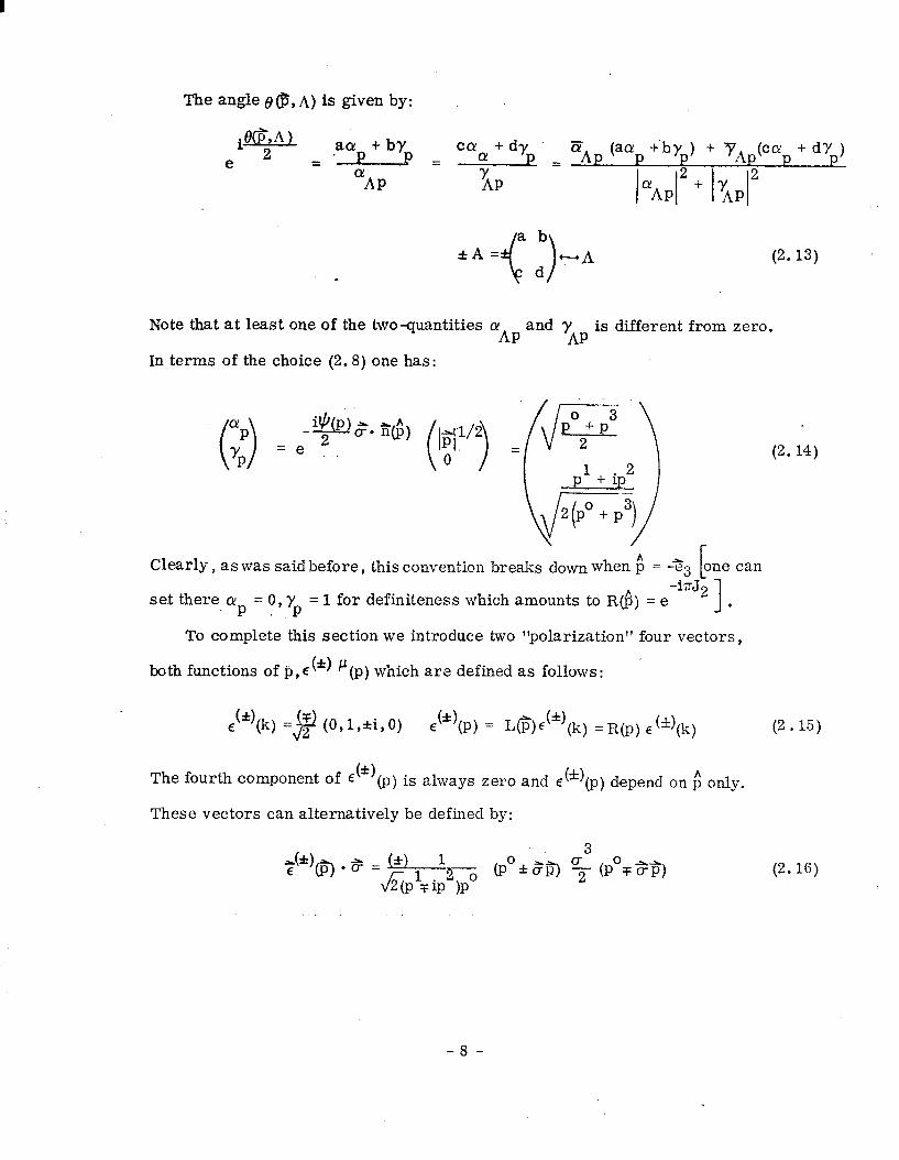
The angle 0 @, A) is given by:
i@SA) 2 e =
.aa + by = CQ~ + dy P /%P
(aa! +‘by ) + ?A (co + dY )
c”hP XP IoAPj2 + /yhp12
&A= ?--+A (2.13) -
Note that at least one of the two-quantities cy and y AP AP
is different from zero.
In terms of the choice (2.8) one has:
cyP
0
a * i@(p) a 2 0-O a?)
?Q =e
( > I I c l/2
0' = d--- PO + P3
2
cp--j 12 + ip
J-
3 qPO+P )
Clearly, as was said before, this convention breaks down when f; = -33 C one can
set there p = 0, yp = 1 for definiteness which amounts td R$) = e Q! -i’ir;li 1 ,
To complete this section we introduce two ‘polarization” four vectors,
both functions of P, E (4 P (p) which are defined as follows:
E (*l(k) =g (0,l ,fi, 0) E(*)(P) = L&c(*)(k) = R(p) E (*)(k)
The fourth component of E &I@) . is always zero and E (5:) (p) depend on f; only.
These vectors can alternatively be defined by:
(2.14)
(2.15)
(2.16)
-8-

Consequently they satisfy the VDxwe11~’ relations :
. O&(f) p E G)=fifTXE d*)@); (2.17a)
from which it follows that:
$*+$-) . ?(f)G) qj .4(f)& = 0 .* (2.17b)
The behaviour of these vectors under Lorentz transformations is quite
interesting. Under a transformation of the little group of k, written 2s:
L-l(Ap) A L(p) = e i0J3 i(xlLl + x94
e
one has:
p = efiec (*k(k)
or
I ii Ac(*)(p p = efie,(*)(*pf -L(X *iX ) (Apy
hi-l2 *
Since the fourth component of E (*t) vanishes this can be rewritten 2s:
We note the appearance of the second term on the right hand side, 2 “gauge
term”. We also remark that the little group angle 8 E e(p ,A) only depends on
(2.18)
the direction of cand not on its maa@tude as was implicit in its eLxpression
(2.13) and is made clear by (2.18).
-9 -

III. WAVE FUNCTIONS AND QUANTUM FIELDS
This section is devoted to the study of free fields describing the creation
and the annihilation of massless particles, and transforming according to an
irreducible representation of the Lorentz group.
Let us introduce the operator a?(,, A) which creates a state ]p ,A>, with
p” = [q , from the vacuum state IO>*
IP,X> =a? cp,x>\o> (3.1)
Note that the choice of phase of the state vector ]p,A> reflects in turn in the
definition of a ‘p, x). The corresponding destruction operator is a@,A). Their
‘commutation rules are:
[ a(p,h)~J(p’~*f ) 1 6
= (27r)3 2p” d3)($- - p“)Q (3.2)
Where 6 = -1 defines the commutator, and 6 = + 1 the anticommutator. The
factor 2p” on the right hand side is dictated by the definition (2.7), which
implies covariant normalization. Finally we have left open the question of the
existence of several states with various helicity X, to take into account possible
discrete symmetries.
The transformation properties of the creation and annihilation operators
under the Poincarggroup follow from those of the states, Eq. (2.12), and the
invariance of the vacuum:
Since U [A] is unitary, we also have:
U [A]a(p ,A)U-l W = e-iXe(pyn)a(Ap, A) (3.4)
- 10 -

By linear superposition of these operators we look now for a quantum field that
transform irreducibly under the homogenous Lore&z group. Let us first
discuss the negative frequency or annihilation part of this field @(-)(x):
9%,X) = s d3p
(2a)32p0 e-ip’Xu(P,h)a(P,h) (3.5)
The field c$(-) . 1s to be thought as a vector in a representation space of some
irreducible representation of the Lorentz group (or rather its covering group),
and the same is true for the wave function u(p,X). Once a basis in such a space
has been chosen we can as well discuss the components @(i)(x) b) and u,(p,x)
of these vectors. The wave function is to be chosen in such a way that
the field transforms covariantly, i. e. , :
U [4]&)(~,h)U-~bf1 = T [4-? @(-)(lzx,A). A (3.6)
In this equation T [A] are the operators of the irreducible representations of,
the Lorentz group. A brief summary of their classification and main properties
has been included in appendices A and B. The reader is referred to them for
the notations to be used below.
It immediately follows from Eq. (3.6) that the wave function has to obey:
u(Ap,h) =e -iAQ(p’ * )T [h] u(p) A)
where 6(p,h) = -6(Ap, 11-l) has been used.
(3.7)
By restricting (3.7) to p = k, where k is the standard momentum of section II,
and ,i to a transformation E of the Euclidian little group of k, we obtain a con-
straint equation for u(k) A), which reads :
T[E]u(k,h) =e ih$(k, E) u(k, A) (3.8)
- 11 -

Setting now p = k and A= L(p) in Eq. (3.7) yields :
u(P,h) = T [L@)]u(k,A) , (3.9)
where we have used 8 (k, L@J)) = 0. This relation, together with Eq. (3.8) ,
ensures the validity of Eq. (3.7). The problem of solving for the wave function
u(p,X) thus reduces to solving Eq. (3.8) for u(k,h).
We shall present two derivations for u(k, X). The first one uses the infini-
tesimal form of Eq. (3.8) and an expansion of u(k,h) in the basis f. Jo-
which
diagonalizes the rotation group. (See appendix A. ) The second uses the techniques
’ and results of appendix B, from which u(k,h) is obtained directly. The latter
method also shows that in the case of infinite dimensional representation Eqs.
(3.6) and (3.7) are in fact improper in a sense to be discussed below, However,
the discussion of finite and infinite dimensional cases proceeds formally in a
similar way.
a. Generator Approach.
Taking the infinitesimal form of (3.8) we obtain :
J3u(k, h) =hu(k,~) (3.10)
L1u(W = L2u(k,h) = o ,
where J3, L1 = KiJ2, L2 = K2 + J1 are the generators of the little group of k
(compare with Eq. (2.6) of the previous section). W-e use the same symbol for a
generator of the Lorentz group and its representative in the representation T.
To obtain the wave function u(p,A) we have only to solve Eq. (3. 10).
To achieve this goal we choose an irreducible representation characterized
- 12 -
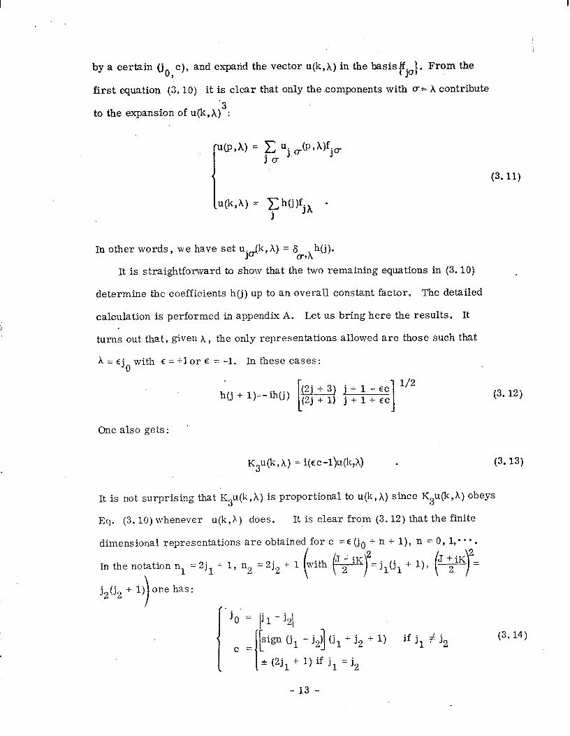
by a certain (j, 9 c), and expand the vector u(k,h) in the basis(fjo/, From the
first equation (3.10) it is clear that only the components with CT= A contribute
to the expansion of u(~,X)~:
In other words, we have set ujJk, X) = ao *h(j). , It is straightforward to show that the two remaining equations in (3.10)
determine the coefficients h(j) up to an overall constant factor. The detailed
calculation is performed in appendix A. Let us bring here the results. It
turns out that, given A, the only representations allowed are those such that
A = Ej with E = +lor E = -1. In these cases: 0
h(j + I)=-ih(j)
One also gets: ~
(3.11)
(3.12)
K3u(k, A) = i(e c -I)u(k,X) . (3.13)
It is not surprising that K3u(k,h) is proportional to u(k,X) since K3u(k,h) obeys
Eq. (3.10) whenever u(k,r) does. It is clear from (3.12) that the finite
dimensional representations are obtained for c = E (j, + n + l), n = 0, 1,. l a.
In the notation nl = 2jl f 1, n2 = 2j, + 1 with \
( .
j,(j, + 1) one has:
‘joe= ij, - j21
iI
c = L si,on tj, - j,) U, + j, + 1) 3 if j, # 1,
* (2jl + 1) if j, = j,
(3.14)
- 13 -

Thus the sign of the helicity x is the one of j, - j,, i. e. x = j, - j, and its
absolute value is given by the lowest “spin” contained in the representation of
the Lorentz group, a well-known result for the case of finite dimensional repre-
s enta tions . 2
Once u(k,h) is known, it is immediate to obtain u(p, A). Using the convention
(2.8), for el;ample, one has:
u(P,U = T[U?9]u(k,A) = R(;)B(lijl )u(k,X)
ON -1) (3.15) =(l? ) wiP(k 9 A) ,
where the Eqs. (3.9), (2.9) and (3.13) were used. Finally, when the wave
function is expanded in the ffja-basis” its components read:
uj&P,x) = h(j) (p”)(EC-l)DL h R(i) , c 1 (3.16)
b. Global Approach
We repeat the previous calculation by usin g the explicit realization of the
operators T b] of appendix B. In other words the vectors C#I (-)(x,x), @,A)
are exhibited as functions of two variables z and Z rather two real variables z+z z-z -- - We write +(-) (z; x,X) and u(z;p,X). Setting:
. . -
Eq. (3.8) ‘akes t.he form:
i
iB
e’z’ i0
p1 -z -ia,) zf e
- 14 -

I .
It is elementary to solve this equation. With h a constant we find: .
u(z;k,A) =hz nl-1 n2-1
2 ,
provided that:
h /la2 2 = Ej
0'
(3.17)
(3.18)
Eq. (3.9) then enables one to find u(z;p, h) which reads:
u(z;P,~) =h(apz + y,) 3-l (crpz'j n2-1 . (3.19)
This compact e.xpression for the wave function has still to be identified with the expres i
sion of its components in the “jo -basisl’. In this form it shows that, when n1 and n2 are
positive integers, the wave function is a polynomial in z , Z, hence belongs to a finite
dimensional representation of the Lorentz group. It also reveals the fact that for all
other cases u(z;p ,A ), and hence Q(z;p ,h ), does not really belong to the space D (n1d-9) l
(See appendix B. ) Finally, as was expected, from (3.19)one sees that u(z;p,h ) depends
only on the spinor (i aP
~. y attached to p (see section II), i. e. , reflects the phase con- P
vention required to define the annihilation operator a@ ,A). Note however, that the
product u(z;ph) a(p,h) is independent of this phase convention. It is possible to expand
(3.19) in the j-obasis. The natural definition uses the scalar product (B.22) in
terms of which one has:
'ju tp) A) <fj&z),u(z;P, A)> =
=h
- 15 -

To evaluate the integral, it is useful to make the change of variables:
Ez’-y P
z=ypzf+cY ’ P
after which the integration is straightforward. One obtiins:
ujq(p, A) = h(j)(p”~c-lD~~ [R&J] , (3.20)
where :
and :
WI% yhp/2 + ,yp,)i12 (“y:: -2) , (3.21)
h(j) = g e l/2
. (3.22)
R($) is the rotation which brings the unit vector in the z-direction to the
direction fi = -- l
T
PI
Equatipn (3.22) yields for h(j +-1)/h(j) the result (3.12), as expected.
One also has ujU(k,h) =aCAh(j), as before.
FinallY we write down a generating function for uj (ph):
j
1 c
j+u j-U Uj&PA) =
Yl Y2
,,jJ(l +u)! tj -aj! Uj,.‘P? A) =
= W )cP’) EC-j-1
h + 3 ! 0 --A)!
(3.23)
This generating function will appear to be useful later.
- 16 -
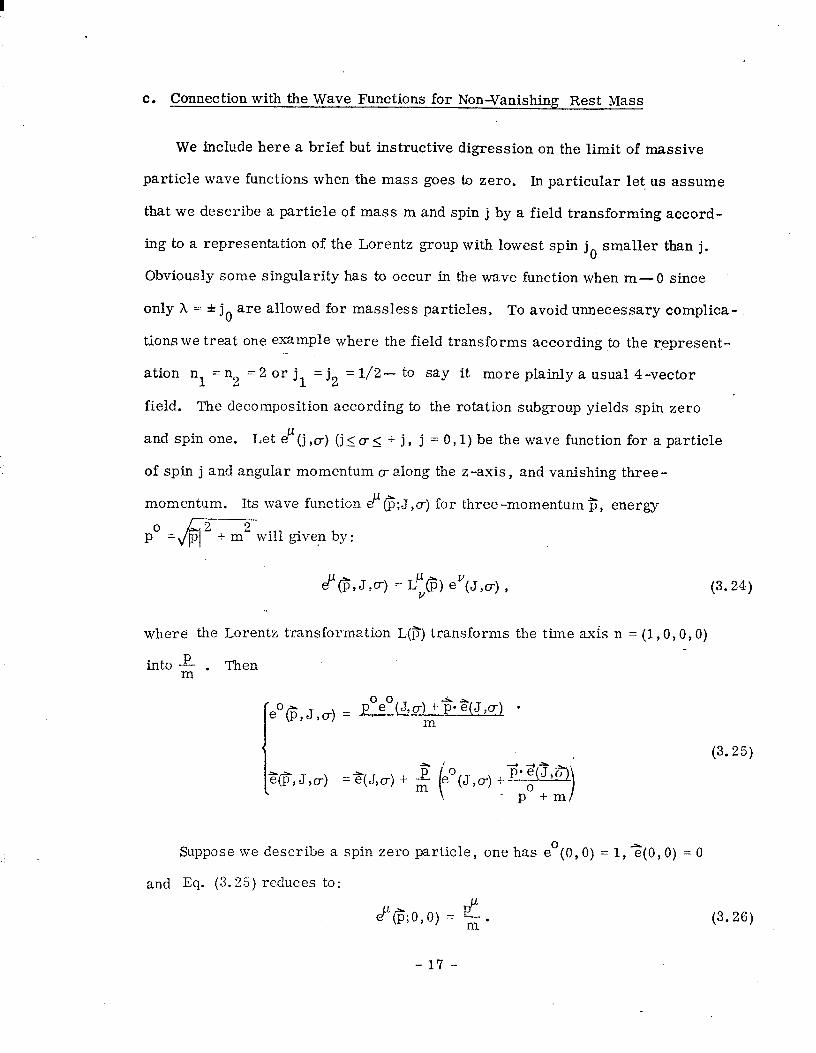
C. Connection with the Wave Functions for Non-Vanishing Rest Mass
We include here a brief but instructive digression on the limit of massive
particle wave functions when the mass goes to zero. In particular let us assume
that we describe a particle of mass m and spin j by a field transforming accord-
ing to a representation of the Lorentz group with lowest spin j, smaller than j.
Obviously some singularity has to occur in the wave function when m-0 since
only A = f j, are allowed for massless particles. To avoid unnecessary complica -
tionswe treat one example where the field transforms according to the rlepresent-
ation n =n 1 2 =2orj 1 =j, =1/2- to say it more plainly a usual 4-vector
field. The decomposition according to the rotation subgroup yields spin zero
and spin one. Let 8(j ,(7-) (j< o- 5 + j , j = 0,l) be the wave function for a particle
of spin j and angular momentum (+ along the z-axis, and vanishing three-
momentum. Its wave function d”(;;,J,u) for th ree-momentum z, energy
p” =&vwill given by:
&$,JP) = $@I eV(J,o-) , (3.24)
where the Lorentz transformation L(p) transforms the time axis n = (1, 0, 0,O)
into z . Then
I e’($,J,cr) = . p”eo(J,c) +Fe $(J,cr) l
m
(3.25)
Suppose we describe a spin zero particle, one has e’(O, 0) = 1, ?(O, 0) = 0
and Eq. (3.2.5) reduces to:
(3.26)
- 17 -

We see that m ec”@,O 0) 4 pc” has a smooth limit when m --+ 0. On the other hand,
from (3.19) it follows that for nl = n2 = S,u(z;p,h = 0) = h(crpz + yp) (EpZ + yp) =
(0)
( -
(1) (2) Z+Z A(z)= lf2” , -2 ,iL$.,
transforms like a four vector under the law A(z)--- (bz +- d) (bz + d) A
can be checked directly, by verifying that
= (bz +d) &?+a) X0 it’ +’ [ [izzT)+qs)*“3
with
A’(z)+;i(z)G? =
Hence the projections of the “spin” zero and “spin” one parts of u(z;p, h = 0)
are proportional to p” and>, respectively, in agreement with the previous limit.
On the other hand-if we start with a spin one particle for which e’(l,u) = 0
we get:
-q$;l,(T) F S(l)@-) -t pql,cJ) p
p” + m m’
(3.27)
Obviously this four vector has no limit as m - 0. However, if we first multiply
by m and then let m go to zero we obtain:
lim m e’(F;l,@ = ;*q 1 ,o-) # m-0 PO
(3.28)
- 18 -

which is a zero helicity wave function. There is no way to obtain the helicity
one wave function for massless particles starting from the j, = j, = l/2
representation of the Lorentz group, as we expected from the general consid-
erations above. In fact this result holds in any spin case. Assume that one
describea massive particle of spin j by a wave function transforming as a
finite dimensional representations of the Lorentz group (n1,n2) with
IL.! Cn2 n +n j,= 2 sjsjnlax=
12 2 -1 = ICI-1 [jmax is thehighest spin in the represent-
ation]. The only non -vanishing finite limit ,when m - 0, is obtained by multiplying the
wave function by m jmax and is proportional to the wave function for a massless particle of
nl-n2 helicity h = 2 , = E j o equal in absolute value to the lowest spin j o.
d. Recursion Relations and Tensor Basis
From the explicit expression for u.#p, X), Eq. (3.20), it follows that one
can relate the various components to each other. Starting from the generating
function Eq. (3.23) we observe that for any positive integer r one has: _ -.. _-. ~.. -.
r
1 = h(j + r)
[ (j + h)!(j -A)!
ii- Ii
*1Y$-Y2
(j+r+h)!(jcr-A)! ’ 1 $2 i(y+~3yly2~ u (y pA)
h(j ) 2 j ,’
.._. (3.29)
- 19 -

. .
and
Thus ‘j&r o- @ , A) is related to u p’@,h). For the case of adjacent j values *
one obtains:
I
Uj+l,cr@‘h)= ‘* kj + l)2-jo{‘bj +a;)(j +(r+ 1) py u~~-~(~,A)
+ Jij + c+ l)(j -u+ 1) i3ujo.(~?4 +
f
1 w- 2
uj -1 ,ir(p, A) = ‘* j2 -jo2 [ I[
J(m) By ujcql(ph)
Al (j+cr)(j+cr+l)p +if;2 u . 2
jo-+ lb, ‘) l (3.32) 1 A single equation, which combines both (Eqs. (3.29) and (3.30), can be
instantaneously derived from Eq. (3.20):
t
-1 ‘ j +n,~(R’) = ‘* [cjh, In/O1 j +nh>l
(3.33)
-20 -
I
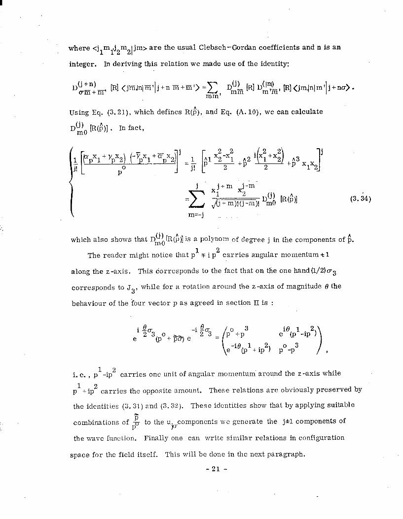
where <j m ,j m jm> are the usual Clebsch-Cordan coefficients and n is an 1 12 21
integer. In deriving this relation we made use of the identity:
.(j +n) Criii+fiF [R] <j.iir,ln]IZfI j +n iii+Iii’> =x
mm’ Dz& [R] Dz!, [R] <jm.@]m’i j +ncr> .
Using Eq. (3.21), which defines R(&, and Eq. (A. lo), we can calculate
D(zo [R($)] . In fact,
! I!! .
1 px1+ ypx2 -JJx1+Tx2 J 1
pY [
Al x2-x1 A2 j! PO
2 2 2 +p =- p ~ j!
i(x;+x:, +;3 xlxl
(3.34)
which also shows that Dmo (j) iR(fi)] . 1s a Polynom of degree j in the components of fi.
The reader might notice that p1 3 i p2 carries angular momentum t 1
along the z-axis. This corresponds to the fact that on the one hand (l/2) u3
corresponds to J3, while for a rotation around the z-axis of magnitude 8 the
behaviour of the four vector p as agreed in section II is :
. 8 el -z”3 0
* 6
@ +EPe -l PiI = P”+P3
i
els(pl -ip2)
evi6(p1+ ip2) p”-p3 ) ,
i. e. , 1 2 p -ip carries one unit of angular momentum around the z-axis while
1 2 p +ip carries the opposite amount. These relations are obviously preserved by
the identities (3. 31) and (3.32). These identities show that by applying suitable
F combirations of pa to the ujcrcomponents we generate the j&l components of
the wave function. Finally one can wri.te similar relations in configuration
space for the field itself. This will be clone in the next paragraph.
-2l-
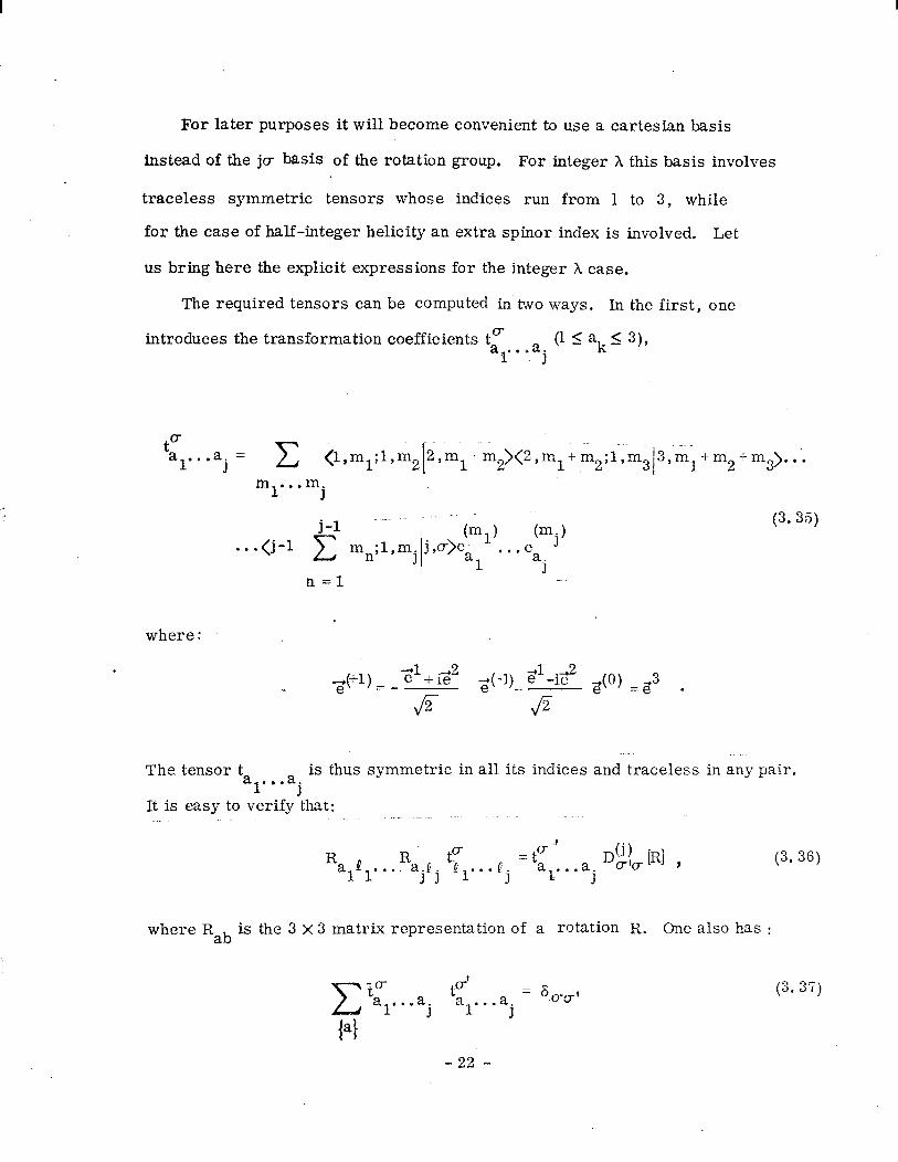
For later purposes it will become convenient to use a Cartesian basis
instead of the ju basis of the rotation group. For integer A this basis involves
traceless symmetric tensors whose indices run from 1 to 3, while
for the case of half-integer helicity an extra spinor index is involved. Let
us bring here the explicit expressions for the integer A case.
The required tensors can be computed in two ways. In the first, one
introduces the transformation coefficients to aTo l o,aj
(1 5 ak5 3),
t” al”*aj = c i l,ml;l,m2 2,ml+m2><2,ml+,m2;l~;m3 3,mY14-m2+m3).... -7 I m . ..m.
1 J
. ..<j-1 2 trnl) tmj)
mn;l,mj j ,o->ea 1
. ..ea. 1
(3.35)
n =l
where :
-+l 3 p)= _ e +iZ” -+(-1)z~1-iZ2 $0) = ~3 .
6 &
The tensor ta . . . a is thus symmetric in all its indices and traceless in any pair. 1 j
It is easy to verify that:
R aP R f-
1 1 . . . . ajtj lil...rj = t” .’
al-* ’ l aj
$1, [RI ,
where R ab is the 3 X 3 matrix representation of a rotation R. One also has :
FJ
-o- t P-’ = al.. e aj al.. . aj 6 -o-CT
u a
(3.36)
(3.37)
-22 -
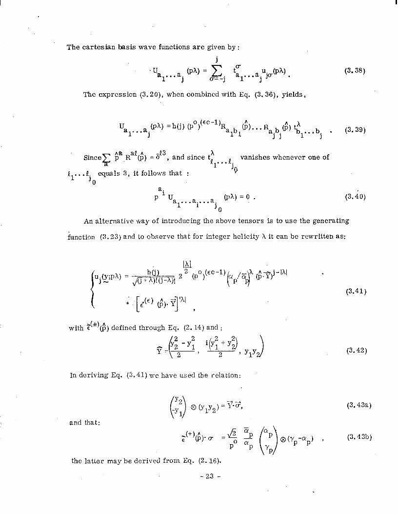
The Cartesian basis wave functions are given by :
(3.38)
The expression (3.20), when combined with Eq. (3.36), yields,
U al’ l l aj
@A) = h(j) (p”)(eC-‘)R albl (“q’*Ra b 6) tl...bj .
j j (3.39)
Since c
$‘,RaQ&) = 8f3, and since th Q1. . . Qj vanishes whenever one of
P1.. . 8. equals 3, it follows that : 8 IO
a. P “a . ..a
1 ie*maj @h)=O. (3.40)
0 An alternative way of introducin, m the above tensors is to use the generating
function (3.23) and to observe that for integer helicity A it can be rewritten as:
(3.41)
with E @) -(*) A defined through Eq. (2.14) and :
In deriving Eq. (3.41) we have used the relation:
(3.42)
(3.43a)
and that:
(3.43b)
the latter may be derived from Eq. (2. .16).
-23 -
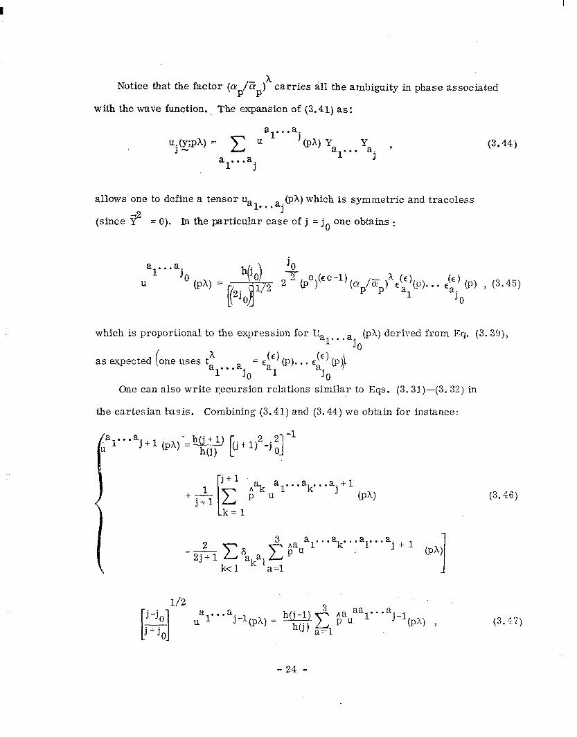
Notice that the factor (crP/EPp carries all the ambiguity in phase associated
with the wave function. The expansion of (3.41) as:
‘j(~Ph) = C ’ al***aj (ph)Ya . ..‘a ) (3.44)
al* ’ “j 1 j
allows one to define a tensor u “1.. .a. (ph) which is symmetric and traceless
5? 3
(since = 0). In the Particular case of j = j, one obtains :
a”‘*ajO hj, 0 j0
U (PA) = 21
c( ll
2 ~(po)kc-l) (@ /z )y)
‘0 P P al(P). l 0 2;) cp) , (3.45)
j0
which is proportional to the expression for ya 1 . . .
i
ajo (ph) derived from Eq. (3.39),
as expected one uses t A a 1 . . .
= p (p). . . P) (p$ ‘j, al ‘j.
One can also write r,ecursion relations similar to Eqs. (3.31)-(3.32) in
the Cartesian b&is. Combining (3.41) and (3.44) we obtain for instance:
2
j+l r %
A% al. . . ak. . . aj i- 1 (ph) P u
Lk= 1
1 +- j+l
0 j-j, [ 1 ual***a.-
3 aa . ..a. J l(ph) = h(j -1)
h(j) a=lp ‘. c ha 1
J-b) , j+j,
(3.46)
(3.47)
-24 -

where we have used:
l--l
m j-j,
j+j,
uj_l(Y;PA) = ‘~
ha 3 [ 1 p af - ujoT;Pq .
The transversality (3.40) of the lowest component follows also from (3.47).
e. General Free Irreducible Fields for Massless Particles
We shall now complete the formulas pertaining to the quantized field. Up
to now we have introduced the annihilation part of the field @(-)(x,X) Eq. (3.5)
and have obtained that if the field transforms according to the representation n -n
T (n1n2)
then h = -$-% Similarly we introduce a positive frequency or
creation part C#I (+I (x, A’) defined as
q(+)(x,p) zz /
d33- e l ipx v(P,Af)bt(p,h’)
. (2rrP(2P0) (3.48)
bt@, A’ ) is a creation operator, which therefore transforms according to (3.3),
U[A]bt@,A’) U-l b] =eih”@‘*)b\fip,AfT) (3.49)
Therefore, by arguments similiar to the case of the annihilation part, the
requirement tba t Q (+) (x, hl ) transforms according to (3.6)) namely by the same
rule as 0(-)(x, A),
U [A] +(+)(x,h’) U% = Tb-1 $(+)(x,h’)
yields that
A’ =n2-nl _c_ zz- 2
A
(3.50)
(3.51)
-25 -

and
. v(p, A” = - A) =c(h) u @,A) 9 (3.52)
where c(h) is a proportionality constant. At this point we have to be slightly more
specific about the physical meaning of the states. If A # 0 then clearly we have
to deal with two types of states, those with helicity A and those with helicity 4.
At the level of Lorentz transformation properties (i. e. , without including
discrete operations like parity P or parity times charge conjugation PC) these
states are distinct so that it is justified to use different symbols like a (p, h),
at@,% b (~4, b’(p) -h) to describe their annihilation and creation. However
when one does not violate any principle by considering coherent superpositions
of the type p]p,A>+~/p, -h>(which is the case of photons but not of pairs neutrino-
antineutrino , due to lepton number superselection rule) it is possible to identify
the operators a and b.’
The full irreducible field now reads
@(x) = &)(x, h) + cp(X, -A)
/
= d3p (2 77)32po
Its transformation law under translations and Lorentz transform.ations is :
~WMWJ+P) = cp(x + a)
u[A]q(x)U+[Al = T [K4 Q(Ax), --y--- - l
nl-n2 -A Pp2) . .
-26 -
(3,54)

-&naiiywecan describe the vector character of G(x) by introducing the variable
z as above. Or we can consider its components in either the tensor or “jc”
basis. We translate here the results, previously obtained for the wave function,
to the field. We limit ourselves to the case of integer h and tensor basis.
Then the lowest component (for A # 0) is divergenceless 3
7 --he (x) = 0. ar= dX%
al,a2...ar...ajo
More generally introducing formally the non-local operator * ‘such that;
6* 55)
(3.56)
we can write the recursion relations as :
a.+1 J ix)rhw --
2. Oal*.*ak***aj+l (xI
axak
i
2 -- 2j + 1 c 6 c
3 d +a,al...ak. .,al...aj+l (x)
” kc1 ak’al a=l axa
3 al...a. h(j-11 d 1
a,a . . ..a. J-+x) = - htjj - -
dX0 A c “+ 1 J--l(x)
a=1 ax
, (3.57a)
(3.57b)
-27 -

IV THE RADIATION GAUGE
Up to now we have extensively discussed the wave functions suitable for
describing massless particles. We have seen that the requirement of Lorentz
invariance restricts the behaviour of the wave function in such a way that it
can only transform according to those representations T Q-y2 )
for which
h =(n 1
-n2) . As a result it seems impossible to describe photons, for
example, by the usual vector potential. Indeed the usual four vector A P
corresponds to the representation with nl = 2, n2 = 2, which accommodates
only helicity zero massless particles and is therefore unsuitable for the descrip-
tion of helicity f 1 photons. On the other hand, the quantization procedure can-
not be applied to the covariant four vector potential without introducing extra
unphysical states. The radiation guage does not suffer from the latter defect,
and is therefore used 4
in quantizin g electromagnetism within the Hilbert space
of physical states. Hotvever, this gauge appears to spoil manifest covariance.
In this section we shall demonstrate that the formalism developed in the
previous section ‘entails that the free electromagnetic field in the radiation
guage transf0rm.s covariantly under a certain infinite dimensional representation
of the Lorentz group. The potential is then the lowest spin component in that .
representation (this result was derived before by Bender 1 using somewhat less
direct methods). In fact we shall show that many apparently non-covariant
transformation laws for potentials of massless particles are indeed covariant,
when those potentials are incorporated in infinite dimensional representntions,
in which the former are the lowest spin components of the latter, All this will
be done for the non-interacting case. The interacting case, which will add nen
structure to the transformation laws, will be treated in another paper.
-28 -
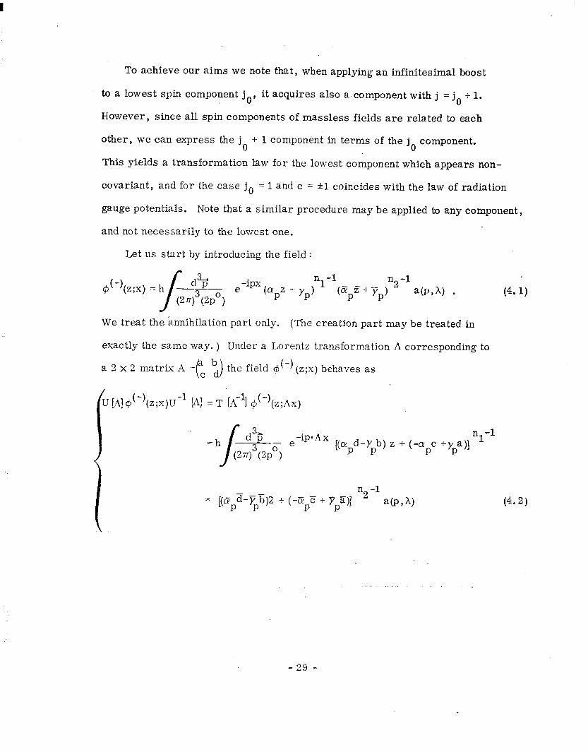
To achieve our aims we note that, when applying an infinitesimal boost
to a lowest spin component j o, it acquires also a component with j = j, + 1.
However, since all spin components of massless fields are related to each
other, we can express the j 0
+ 1 component in terms of the j, component.
This yields a transformation law for the lowest component which appears non-
covariant, and for the case j, = 1 and c = *l coincides with the law of radiation
gauge potentials. Note that a similar procedure may be applied to any component,
and not necessarily to the lowest one.
Let us start by introducing the field :
et-)(Z;X) =h -r---
/
cl%
(2T) (2PO) emipx (a z + y
P P jnl-l(h z + 7 Jn2-1 a(P A)
P P , . (4.1)
We treat the annihilation part only. (The creation part may be treated in
exactly the same way. ) Under a Lorentz transformation A corresponding to
a 2 X 2 matrix A = the field @(-),(z;x) behaves as
[A] +(-)(z->-)U-’ [A] = T L-A-4 $(-)(z;Ax) , L
I( /
=h d3ij e -ipnAx [(Qpd-Ypb) z + (-orpc -typa)] nl-1
(27-r)“(2p0)
* [(apZ-ijip’;)Z + ( -BpE + 7 P
ST)] n2 -’ a @ , h) (4*2)
-29 -

The transformed field is given by the same formula as (4.1) with
x-Ax and Defining the generating field:
@(-I (y;x) =
i
j cc
* @JpY1 + YpY2) j++-lY1 +s Y) p 2%lp,h)~
we get, combining formulas of the previous section with Eq. (4.2),
U [A] +i-’ (~-;lc)U-’ [A] = h(j) [{ j + A) ! (j-h)!] -l/2
(4.3)
(4.4)
Clearly if ~1 is a rotation we obtain the ordinary behaviour corresponding to the
representation j of the rotation group. On the other hand for Pure Lorentz
transformations we find, for j = j,,
i K [ a’ ~j,'y;"'] = (so~a-xaaO)~jo (~;“>
(4.5)
+ l/2 e(y%avy)pj,(.y;x) + (j, + l-cc) 3%A ~$~,(s’;x)
-30 -

I
where we remind the reader that T -l/26. g is identified with e B.“K
(see
appendix B). We also note that when q(x) transforms by T nln2 ’ dO9(x)
transforms by Tn + 1 n + 1 as is clear from (4.4). 1 ‘2 ’
For the case of integer j,, combining (4.5) with (3.41) and (3.44) gives
bI . ..b. = (x”aa-xaao) Q JO (xl
- (j, + 1 -EC) q $ bI.. . b.
‘0 w
j0 bl...bk-lb’bk+I...b. -ie
c ‘0
k=l “gbKb’
@ w ,
(4.6)
where in the course of the calculation, it is useful to realize that:
It can be verified, using Eq. (2. ISa), that the right hand side of E,q. (4.6)
is transverse in b . . . b. , as it should. 1 JO Using the same equation one also gets:
abc bI...bk Icbk+I...b.
JO bI...b
k-labk+
(ie)E G 1’ l l bjo
(x)
(4.8)
-31 -
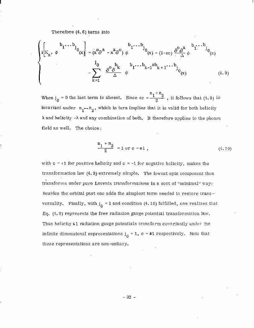
Therefore (4.6) turns into
([ bl...b.
JO zz c;Paa -xaao) + bl.. .b.
iK a’ @ 6 JO (X)
(4.9)
n +n When j, = 0 the last term is absent. Since EC =v , it follows that (4.9) is
invariant under n ++n 1 2’ which in turn implies that it is valid for both helicity
A and helicity -A and any combination of both, It therefore applies to the photon
field as well. The choice :
n1 i-n 2 2 =lorc =*I, (4.10)
with c = +l for positive helicity and c = -1 for negative helicity, makes the
transformation law (4. 9.) extremely simple. The lowest spin component then c
transforms under pure Lorentz transformations in a sort of “minimal” way:
Besides the orbital part one adds the simplest term needed to restore trans-
versality. Finally, with j, = 1 and condition (4.10) fulfilled, one realizes that
Eq. (4. 9) represents the free radiation gauge potential transformation law.
Thus helicity *1 radiation gauge potentials transform covariantly under the
infinite dimensional representations j, = 1, c = *l respectively. Note that
these representations are non-unitary.
- 32 -

V. COMMUTATION RELATIONS
In this section we investigate the commutation rules among the various
field components. Let the field be expressed as:
\ * i”pYl +YpY2d+h(-j;pYl+~pY2~-A* [e-iPxa(p,h)+c(X)eip~~~, -A)]. (5.1) .._ . . - _ -- -- - . . __ .~
The commutation rules among the creation and annihilation operators are :
[a$,h),&pW)]k = b@,~),b~(p1,~f)]8 = (2q3(2p0) s,,,~(~)&p) (5.2)
with[A,B]* =AB + 8BA, and 8 =*I. All other commutation relations vanish
(the treatment of self-conjugate particles, namely a(p, h) = b(p, h), does not
yield any new results. In fact, there need not be separate treatment for self-
conjugate particles whenever h # 0, since then a (p, A) and a (p, 4) commute t
(or anti -commute) . One therefore readily obtains :
19jt~ix), ~j’ ‘-“‘;“‘)I* = [$ (YP), $-, (y’;x’)j* = 0 /5* 3)
However, the commutator [$j(y;~), #i, (y’;x’)lg does not vanish. It is:
*a /
d3F AX’
(2n)3(2Po) ) - tj+j’+zfl
* @pY1+YpY2)j+h -- .‘+A
t l.yl+ 5pY2$-sEpY; +YpYg , j’-A
(-y y’+cY Y ) pl p2
-33 -
I
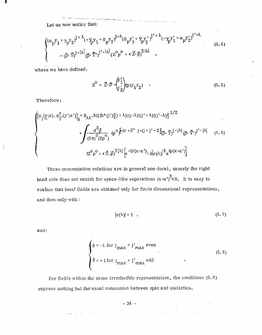
----~_. Let us now notice that:
where we have defined:
z” + g*e ;
0 ,f S(Y,Y,) ’ 2
(5.5)
Therefore :
o:,(Y’;x’)J~= $,,h(j)h*(j’)[(j + h)!(j-A)!(j’+ h)!(j’-A)iJ l/2
These commutation~relations are in general non-local, namely the right
hand side does not vanish for space-like separations (x-x’)‘<O. It is easy to
realize that local: fields are obtained only for finite dimensional representations,
and then only with :
Ic(h)l=l ,
and:
i
6 = -1 for jmax + jImax even
6 = + lfor jmax f jfmaY odd d .
(5.7)
For fields within the same irreducible representation, the conditions (5.8)
express nothing but the usual connection between spin and statistics.
- 34 -

For the free radiation guage electromagnetic potentials Aj(y ;x) one has
EC =EC r = 1, lq = 1 and hence
[Aj(~;X) ,A:,(~ -
‘;x’j) =h(j)h (j’)ej+l)!(j-l)!(j’+l,!(j’-l)! l/2
x sin p’ (x-x’)
For the lowest components:
~l(~;x),A$y’;~‘)J =; (Z”+ E%! ,2 sin pa (x-x’). N P
The equal time commutators between two fields or a field and its time
derivative are then:
(5.10)
(5. lla)
(5. llb)
as expected. The first commutator vanishes when fields which include both
helicities are used.
- 35 -

APPENDIX A
THE LORENTZ GROUP-GENERATOR APPROACH
In this appendix we recall, for completeness, the action of the Lorentz
generators in the ‘ljtir basis, namely the basis which diagonalizes rotations, 5
and then solve for the coefficients h(j) of the wave function u(k,A) (see Eq. (3.11).
A more formal treatment of the representation theory. is given in the next
appendix.
The generators of rotations 5 and Lorentz transformations (boosts) I(’ obey
the commutation rules:
Let fj,be basis “states” which diagonalize rotations, namely,
J2 fjo = j(j + 1) fjo
and
“ifjo = Jjcjfl,-a(ort 1) fjtil
i
J3 fjo =ofjV
From the vector character of I? under rotations and
follows
(A. 2)
(A. 3)
K f. =a f + J” jU j-IV+ I+ bpfju+ I+ ‘jOfj + la+ 1
-36 -

The dependence
straightfonvard
of the coefficients a ja’ Jo-
b. and cP on ocan be determined
calculation using J+,K+ = 0. One then gets : [I I Kf + ju=aj~~)fj-lu+l+bj~ja)(j+u+l)fju+1-cj~(j+~+1)(j+~+2)f. J+hJ-+I
.-.
The faction of K3 is determined by that of K+ and K+, J- = 2K3, and that of K- [ 1 from that of K3 and = K, We thus get:
wl( j ~+l) fj -lu*l + bj Jib) (j*u+l) fjukl
(j*u+2) f. J+ 1Uk.l I
K3fjc = aj hvfjwlu + bju fju + cj ,/jj fj+lu .
(A.9
J.ZI a certain irreducible representation, 3. d = p and j2 - Z2 = s are
constants.
Thus,
,./ . ,. ., ._ ._ :-- -.. - --. implies :
while :
(?* i?) fjj = Pfjj . .
.1--. ._
b/P ; 3 jtj+l)
(f _R2)fjj = sf jj ,
implies :
where :
2 s = j(j+2) - ’
U+ V2 - Nj(2j+l) (2j+3) ,
Nj =a. JflCj .
-37 -
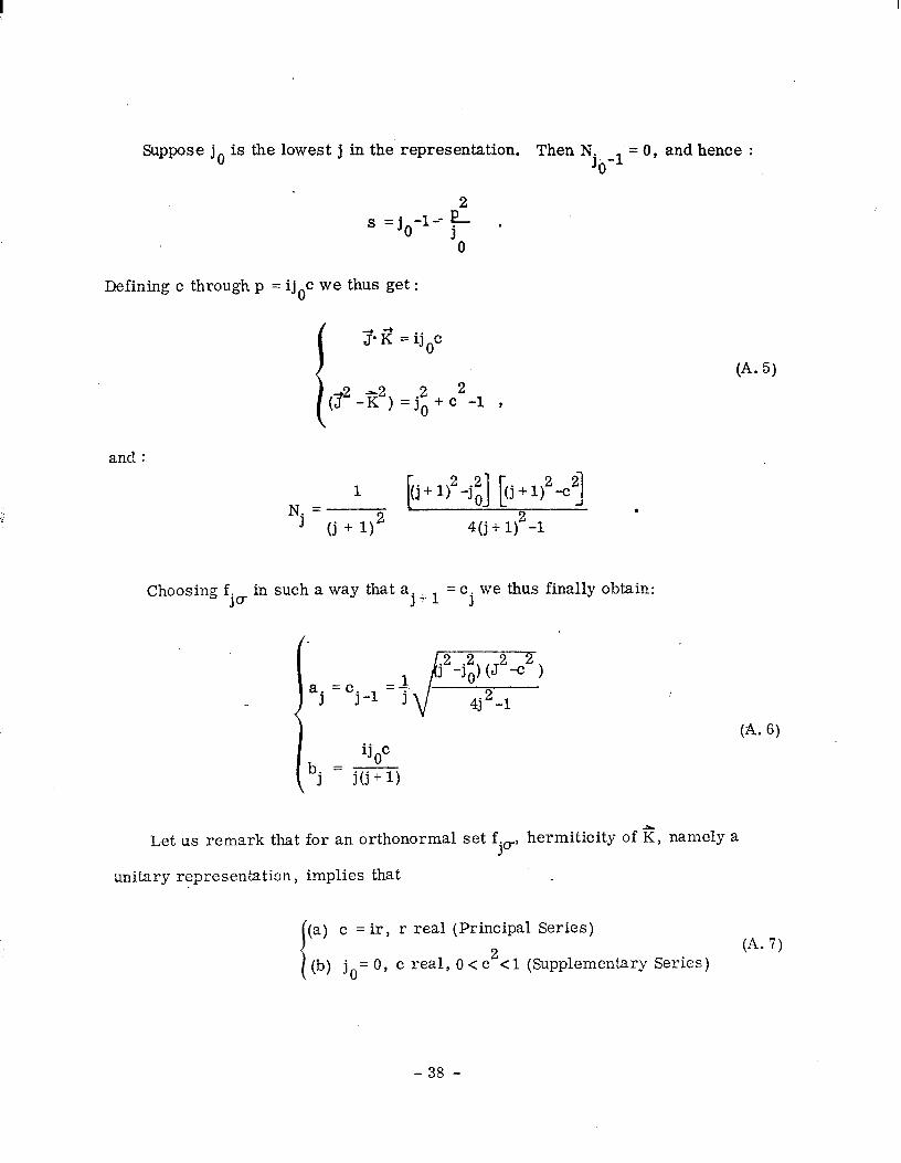
Suppose j, is the lowest j in the representation. Then N. lb-1
= 0, and hence :
s =j -14 2 0 j l
0
Defining c through p = ijoc we thus get :
I
J*l? = ij,c
(j2-z2) =jE+C2-l ,
and :
1 Nj = j+l)2-j:] [(j+l?-c2 1
tj + II2 4(j + 1)2-1 .
(A- 5)
Choosing f. J’T
in such a way that a. I+1
= cj we thus finally obtain:
ij c bj = --!!-
j(j + 1)
Let us remark that for an orthonormal set f. Ju, hermiticity of 2, namely a
unitary representation, implies that
i
(a) c = ir, r real (Principal Series)
(b) j,= 0, c real, 0 < c2<1 (Supplementary Series) (A* 7)
-38 -

The finite dimensional representations are obtained for /cl = j, + n + 1,
n =0,1,2,... For those , den.oting :
_. -.-- --.. ._ ___. . 2
Z-i< () 2 =j,tj, + 1) ( ) J’+ iz
2
2 = j, (j, + I), !
one obtains :
for j, # j,
For a more complete discussion the reader is referred to the literature. 5
(See also Appendix B ;)
We now proceed to solve the constraint Eqs. (3. lo), which read:
J3u(k,h) = Au(k,A)
(K--iJ-) u(k, h) = 0
(K+ + iJ+) u(k,h) = 0 l
It is straighforward to show that Eqs. (A. 10) imply :
i
(?- z)u(h) = h(K3 + i)u(A)
@2-82)u(h) = [A2-l-(K3 + i)2]u(h) .
(A* 8)
(A* 9)
(A. 10)
(A. 11)
- 39 -

., . . . __
Thus, in an irreducible representation (j,,c),
X(K3 + i) u(h) = (ijoc) u(h)
i
(K3 + i)2 u(A) = (A2-ji+2) u(h)
It thus follows that one necessarily has :
(A2-jo2) (X2-c2) = 0 l
(A. 12)
.
(A. 13)
Hence either A = ejo or h = EC (obviously, the latter is valid only for j,-c
integer). It turns out that h =EC does not give any solution not included already
in the A = Ej case. Thus one has 0
i;. u(; ::;c-1) u(A)/ ‘=*I.
(A. 14)
The derivation of (A. 14) from (A. 12) is not direct for h = 0. However,
Eqs . (A. 14) holds in general.
Using Eqs. (A. 3) and (A.4) and the expansion (3. ll), one can solve for the
coefficients h(j) from Eqs. (A. 10). The solution is:
h(j + 1) = -ih(j) (A. 15)
-40 -

I
APPENDIX B
SUMMARY OF REPRESENTATION THEORY FOR SL(2C)
In this appendix we give a brief survey of the representation theory for the
group SL(2C), the covering group of the homogeneous Lorentz group. This is
mainly to define the notations, and to derive some identities used in the text. We
rely mainly on the classical reference texts from Naimark, Celfand and coworkers. 5
The results are first stated inglobal form; then, using a particular basis to diag-
onalize the SU(2) -subgroup, they are also given in the Lie-algebra or infinitesimal
form.
To describe the representations one introduces function-spaces D (np “2)
with
nl, n2 two-complex numbers, such that nI-n2 is an integer. A function of two real
variables x, y are conveniently grouped as z = x -t iy, < = x - iy so that a
function of the variables x, y is also written f(z, y) belongs to D ) $2 9
if
(i) f(z, z) is infinitely differentiable (in short Cm )
(ii) ?(z, 2) = z nI-1 n2-1
Z f(+; ) is also C30.
One abbreviates f(z, y) by f(z). The topology on D (y n2Y
namely uniform conver-
gence of f and .! and their derivatives on compact subsets of the z-plane, will not
be discussed here except to state some results.
In the space D (“y 3)
-one defines a continuous representation of SL(2C) through
the following relation. For any two by two matrix A of determinant one sets A-
T(A) where the linear operator T(A) acts in D P-y n2>
as follows :
i
f(z)-[T(A)f] (z) = (bz + d)nl-’ (h;+d)n2-1 f (;; 1 c,)
(rs. 1)
-41-

These representatians exhaust in a certain sense all irreducible representations
of SL(2C). We summarize irreducibility and equivalence by distinguishing the
situation of ?ntegerl* and “non-integer” (n,, n2) points as follows: An index (n,, n2)
is said “integer” if (nl, n2) are both non-zero integers of the same sign.
Non-integer Points
The representation at a non-integer point (nln2) is irreducible. Two repre-
sentations (nl, n2) and (nip 2 n’ ) are equivalent if and only if ni -t- nl = ni + n2 = 0.
Equivalence means the existence of a continuous, invertible intertwining operator
between D @ 1' n2)
and D (n ' 1' "8,'
Irreducibility is understood as:
(i) subspace irreducible: no closed proper invariant subspace
(ii) operator irreducible: all-continuous operators committing with the T(A)
are multiples of the identity.
All these representations are infinite dimensional. They contain in particular
the important special case of unitary representation.
Unitary Representations \
They fall into..two series.
(i) Principal series characterized by nl f x2 = 0 or
nl=+(n+ip) n integer, p real
n2 = $ (-n I- ip) ,
with scalar product: --
(f, g) = ;I+- dzdz f(z) g(z),
The measure is: $- dzdz = dRez dtmz.
(ii) Complementary series characterized by -
nl =n 2= c, -l< c<l, c# 0,
(Be 2)
(Be 3)
(B-4)
-42-

and scalar product (valid for -l<ccO; the representations with O<c <l are
equivalent to those with -l<c CO, since n 1 = n2 = c and n = n = -c are equivalent). 1 2
(f, g) = ($f{($ dzl dil k2 d-2 lzl-z2 (_ 2c - 2 i(z,t g(z2) (B. 5)
Integer Points
These representations are no-more subspace irreducibles though they are still
operator irreducible. In fact, with nl, n2 both positive integers, the four repre-
sentations T nl, n2’
T -nl, n2 ’ Tn, p2
, and Tvn 1’ -n2’
are related by various continuous
mapping which commute with the operations of SL(2C). Consequently the kernels
and images of these mappings are invariant subspaces. Denote by E the closed nl, n2
subspace of D nl, n2
of polynomials in z, z of degree at most nl-1 in z, and n2-1
in z. This is an invariant subspace of D . Similarly let Fen be the sub- nl, n2 _ Yn2
space of Den Yn2
of those functions f which satisfy:
J d dzd: j-k z z f(z) = 0, for O<j<nl-1, Olk5n2-1 .
This is a closed infinite dimensional subspace of Dsn 1, -n2’
Note that E is nln2
finite dimensional (dimension nlxn2) and carries the usual finite dimensional
, representations of SL(2C). The indes (nl, 2 n ) can be written (Zj, + 1, 2j, + 1) to
make contact with the usual notation where T-i? is represented by spin j 1 and
T-f-i?? by spin j, (see below).
Let the symbol cv denote isomorphism between spaces and equivalence between
representations in the corresponding spaces. Then one has :
D E /
-F -D -D nl, “2 nl, n2 _ -n19 -n2 -nl,n2 nl,-n2
D F -E _ 1’ -n -n2
/. -n -n 1’ 2 n1,n2 . (B. 6)
-43-

Infinitesimal Form with ei(ZZi +$I?) for ?and ?j infinitesimal we
derive the expressions of the generators r and ?? in the space D . They read:
-
Pl’ nz)
2 a ) z -
1)~ + (n2-1)Z - (1 + z )az 2Q1+$& I
i
(n2-1)” + (l-z 2 -@. + (l-z )az -23 )Fz I
(n2-1)Z + (1+z2)& - -2 a (l+z )a? I
(Be 7)
The usual invariants take the following values with nl = 2jl+ 1, n2 = 2j, + 1
= i(T)r11n2) (B-8)
The Rotation Basis
Except for the cases corresponding to the unitary representations, the vector
spaces D by) 3)
are not naturally equipped with a bilinear form, However, they
carry a reducible representation of the compact group SU(2), which we expect to
be equivalent to a unitary one-direct sum of the well known representations of
“spin*’ j. We shall indeed construct in D @lJ 3)
a bilinear form invariant under
W(2), which allows to embed D @lG4
as a dense subspace of a Hilbert space, a
basis of which diagonalizes the representation of this group.
-44-

We proceed by constructing sets of 2j + 1 functions fjQ(z) belonging to D
such that the subspace spanned by these functions is left invariant under the (nlT n2)’
action of T (n n )(A), for A restricted to SU(2). 12
We are thus looking for fj,(z) with the property that for A restricted to SU(2):
where the Wigner functions D (j) (A) due
are defined by:
5.’ = ATx
(B. 9)
(B. 10)
Combining (B. 9) and(B. 1) we get
nl-l (E + a) (z) Df/c (A)
A=6 ;)=@ -3 (B. 11) ,
To solve for’fjo(z) from (B. ll), one simply chooses a matrix A such that az + c = 0,
for example :
thus obtaining :
:. fju, (Z)D~~ (AZ,) = (1 + Z~) 2 - ’ fju(0) ,
(B. 12)
(B. 13)
-45 -

I
It remains to compute . fjo( 6). TO this end we note that, choosing A = em- - in
tj). (B. ll), and using DotO. = 6 i&r cr ‘u
e , one gets
and hence:
fjC(0) = fj 6 .n2-nl l
=,2.
It thus follows that n +n 1 2-1
fjo(Z) = fj(l + ZZ) 2 D(j) n2 -*1 - ,cr 2
(B. 14)
(B. 15)
Defining ‘the initary matrix Vz by
Kz = Vz(io2)
we obtain n fn 1 2 fjo(Z) = gj(l 4 ZT) 2 -’ D(j)
,f1-“2 (vz)
2
vZ (B. 16)
. n-n 2 1
where g. =; j+ 2
J fj(-) and where Do,o(io2) = (-) j -Wt8 u,, u has been used.
As will become clear later, it is convenient to choose:
Let us now introduce the following generating function:
+j z 4 Q=-j
(B. 17)
. nl-n2 nl-n2
(Xl z + x.9 2 (-x1
gj&-)
-j-r + x2z)
-n - nl-n2 n +n
2 ‘J -- 2 !(I + zzj'j+l- ’ 2 2
, (B. 18)
-46-

I
This definition requires of course (in order to have a homogeneous polynomial of
degree 2j in 3 that a nl-?2
j-j,-- 2 I I be a non -negative integer (B. 19)
The lowest “spin” contained in the representation will thus be j,. We now verify
that fj,have indeed the required properties.
(i) fjcr(z) is clearly CQ), as is t,(z), since t,(z) = (-1)J +“fjc(z) or
-denotes an element of W(2) so that V-l = V+, det V = 1 or
then according to (.B-1):
T(nln2) ( V)fj(~’ z) = fj(V~, z), (B. 20)
where we have used the fact that unitarity of V implies that (1$$])2 = ;b; ‘:z2 .
From this equation it immediately follows that the fjP(z ) obey Eq. (B-9).
Apart from a factor; we observe that fjfl(z) is a DJ-function. we can thus set
up a hermitian “scalar producP in D @l, “2,’
invariant under SU(2), such that with
respect to this scalar product fj&z) and f j,cr,(z) will be orthogonal for (j,,) # (jt,ct).
We shall indeed show that one has:
2 - s
- wn1+ n2L
rr +lzdY(l+z;) _ fj,(z)fjt,t(z) = ~jjt 6a-at
r(j + l- T2) -.
(B 21) n +n .
l2 2
i0 e To prove this relation we set z = e ctg2 3 OSPSn and remark that f. JP
eiHk’P’f P
(ctgs), and further tha.t* .
cos v = E E -sin--
NT-Z 4 i I sin2 e ;’ cos-
-47 -

Hence with the classical notations of quantum mechanics textbooks :
I+ ( )
. “l-*2 -3’ “,,,$ = 5-n2 m2
2
the left hand side of (B, 2 1) reads:
. where we have used the orthogonality properties of the dJ functions.
Let us briefly comment on the scalar product derived from (B. 21). For any
two f and g belonging to D the following integral obviously exists: Fly 3)
<f,g> = ; s
; d,zdz (1 + z; ) -w*l+“2) _
f tz Mz 1 =
(B. 22)
(The use of the< , > notation is to distinguish this scalar product from that introduced
before), Clearly < f, f >r 0 and the equal sign only holds for f = 0. Dtn 1’ n2) is not
complete with respect to this norm but is dense in its completion, a Hilbert space that
we can denote H tn17 n2)’
It is easy to see that the set fjC (z) is an orthogonal basis
in this space (jaj, no*negative integer). It is gratifying to observe that the scalar
product (B. 22) is precisely the one corresponding to the principal series, since from
n +n2- - - 0 follocys Re(nl -i- n 1
2) = 0 (compare with B. 3) and in this case:
r((j+l-q] = 1.e
nli n2 2
-48 -

However in the case of the supplementary series,(B. 22) does not coincide with (EL 5).
Indeed one can easily verify that for n1 =n2 = C, -l<c<O the following identity holds,
and since 2c = nl + n2 = Re(“l+nJ
tfj ,U”fju) = 2(-1)j+1 r(c-j)r(l+c +~’ btl+c ,3
<fjrar, fj~> = 2T(-C)/T(1+C)S,,sjjl
nl 2 =n = C,-l<C CO. j, jT = 0, 1, . . .
Thus apart from an overall constant factor the functions f. JU are again in that case
an ortho-normal basis for the unitary representations of the complementary sense.
This explains the particular normalization choosen above,
Let us exhibit the action of the generators?, ?iz on the functions fj,(z). With
K, = ,Kl*iK2, they read
J* fjo = J(jro-)(jktcr+ 1) fj o&l >
where we have used the notations of Naimark
(B. 24:
‘In1-n21 n -t n j,= c = sign (nl-n2) 1 2
n 3-n or f 1 2 if = ,
2 2 2 nl n2. (B.25)
-49 -

I
1
ACKNOWLEDGEMENTS
This work was initiated by fruitful discussions with Professor Henry Don
Itzhak Abarbanel. The authors are also indebted to him for continuous encourage-
ment without which this work would not have been completed.
-50 -
I
REFERENCES AND FOOTNOTES
1. C. M. Bender, Phys, Rev. 168, 1809 (1968).
2. S. Weinberg, Phys. Rev. 134, B882 (1964).
3. We donotspecify convergenceproperties here. We only require that h(j)
be finite. From the solution (3.12) it follows that h(j) -+l as j+co.
4. J. D. Bjorken and S. D. Drell, Relativistic Quantum Fields, (McGraw Hill,
N. Y. , 1964).
5. For the theory of representations of the Lorentz group see: M. A. Naimark,
Linear Representations of the Lorentz Group, (Pergamon Press, N. Y. ,
1964), and I. M. Gelfand, M. I. Graev, N. Ya-Vilenkin, N. Y. , Generalized
Functions, 2 (Academic Press, N. Y. 1966).
- 51 -
Top Related