Work supported in part by US Department of Energy contract DE-AC02-76SF00515.

THE ATACAMA COSMOLOGY TELESCOPE: COSMOLOGY FROM GALAXY CLUSTERS DETECTED VIA THESUNYAEV-ZEL’DOVICH EFFECT

NEELIMA SEHGAL1, HY TRAC2,3, V IVIANA ACQUAVIVA 4,5, PETERA. R. ADE6, PAULA AGUIRRE7, MANDANA AMIRI 8,JOHN W. APPEL9, L. FELIPE BARRIENTOS7, ELIA S. BATTISTELLI 10,8, J. RICHARD BOND11, BEN BROWN12, BRYCE BURGER8,

JAY CHERVENAK13, SUDEEPDAS14,9,4, MARK J. DEVLIN 15, SIMON R. DICKER15, W. BERTRAND DORIESE16, JOANNA DUNKLEY 17,9,4,ROLANDO DÜNNER7, THOMAS ESSINGER-HILEMAN 9, RYAN P. FISHER9, JOSEPHW. FOWLER9,16, AMIR HAJIAN11,4,9,

MARK HALPERN8, MATTHEW HASSELFIELD8, CARLOS HERNÁNDEZ-MONTEAGUDO18, GENE C. HILTON16, MATT HILTON19,20,ADAM D. HINCKS9, RENÉE HLOZEK17, DAVID HOLTZ9, KEVIN M. HUFFENBERGER21, DAVID H. HUGHES22, JOHN P. HUGHES5,

LEOPOLDOINFANTE7, KENT D. IRWIN16, ANDREW JONES9, JEAN BAPTISTE JUIN7, JEFF KLEIN15, ARTHUR KOSOWSKY12,JUDY M. L AU1,23,9, M ICHELE L IMON24,15,9, YEN-TING L IN25,4,7, ROBERT H. LUPTON4, TOBIAS A. M ARRIAGE4,26,DANICA MARSDEN15, KRISTA MARTOCCI27,9, PHIL MAUSKOPF6, FELIPE MENANTEAU5, KAVILAN MOODLEY19,20,

HARVEY MOSELEY13, CALVIN B. NETTERFIELD28, M ICHAEL D. NIEMACK 16,9, M ICHAEL R. NOLTA11, LYMAN A. PAGE9,LUCAS PARKER9, BRUCE PARTRIDGE29, BETH REID9,30, BLAKE D. SHERWIN9, JON SIEVERS11, DAVID N. SPERGEL4,

SUZANNE T. STAGGS9, DANIEL S. SWETZ15,16, ERIC R. SWITZER27,9, ROBERT THORNTON15,31, CAROLE TUCKER6, RYAN WARNE19,ED WOLLACK 13, YUE ZHAO9

Draft version October 7, 2010

ABSTRACTWe present constraints on cosmological parameters based on a sample of Sunyaev-Zel’dovich-selected

galaxy clusters detected in a millimeter-wave survey by the Atacama Cosmology Telescope. The cluster sam-ple used in this analysis consists of 9 optically-confirmed high-mass clusters comprising the high-significanceend of the total cluster sample identified in 455 square degrees of sky surveyed during 2008 at 148 GHz. Wefocus on the most massive systems to reduce the degeneracy between unknown cluster astrophysics and cos-mology derived from SZ surveys. We describe the scaling relation between cluster mass and SZ signal witha 4-parameter fit. Marginalizing over the values of the parameters in this fit with conservative priors givesσ8 = 0.851±0.115 andw = −1.14±0.35 for a spatially-flat wCDM cosmological model with WMAP 7-yearpriors on cosmological parameters. This gives a modest improvement in statistical uncertainty over WMAP7-year constraints alone. Fixing the scaling relation between cluster mass and SZ signal to a fiducial relationobtained from numerical simulations and calibrated by X-ray observations, we findσ8 = 0.821± 0.044 andw= −1.05±0.20. These results are consistent with constraints from WMAP 7 plus baryon acoustic oscillationsplus type Ia supernoava which giveσ8 = 0.802± 0.038 andw = −0.98± 0.053. A stacking analysis of theclusters in this sample compared to clusters simulated assuming the fiducial model also shows good agreement.These results suggest that, given the sample of clusters used here, both the astrophysics of massive clusters andthe cosmological parameters derived from them are broadly consistent with current models.Subject headings:cosmic microwave background – galaxies: clusters: general – cosmology: observations

1 Kavli Institute for Particle Astrophysics and Cosmology, Stanford Uni-versity, Stanford, CA, USA 94305-4085

2 Department of Physics, Carnegie Mellon University, Pittsburgh, PA15213

3 Harvard-Smithsonian Center for Astrophysics, Harvard University,Cambridge, MA, USA 02138

4 Department of Astrophysical Sciences, Peyton Hall, Princeton Univer-sity, Princeton, NJ USA 08544

5 Department of Physics and Astronomy, Rutgers, The State Universityof New Jersey, Piscataway, NJ USA 08854-8019

6 School of Physics and Astronomy, Cardiff University, The Parade,Cardiff, Wales, UK CF24 3AA

7 Departamento de Astronomía y Astrofísica, Facultad de Física, Pon-tificía Universidad Católica de Chile, Casilla 306, Santiago 22, Chile

8 Department of Physics and Astronomy, University of BritishColumbia, Vancouver, BC, Canada V6T 1Z4

9 Joseph Henry Laboratories of Physics, Jadwin Hall, Princeton Univer-sity, Princeton, NJ, USA 08544

10 Department of Physics, University of Rome “La Sapienza”, PiazzaleAldo Moro 5, I-00185 Rome, Italy

11 Canadian Institute for Theoretical Astrophysics, University ofToronto, Toronto, ON, Canada M5S 3H8

12 Department of Physics and Astronomy, University of Pittsburgh,Pittsburgh, PA, USA 15260

13 Code 553/665, NASA/Goddard Space Flight Center, Greenbelt, MD,USA 20771

14 Berkeley Center for Cosmological Physics, LBL and Department of

Physics, University of California, Berkeley, CA, USA 9472015 Department of Physics and Astronomy, University of Pennsylvania,

209 South 33rd Street, Philadelphia, PA, USA 1910416 NIST Quantum Devices Group, 325 Broadway Mailcode 817.03,

Boulder, CO, USA 8030517 Department of Astrophysics, Oxford University, Oxford, UK OX1

3RH18 Max Planck Institut für Astrophysik, Postfach 1317, D-85741 Garch-

ing bei München, Germany19 Astrophysics and Cosmology Research Unit, School of Mathematical

Sciences, University of KwaZulu-Natal, Durban, 4041, South Africa20 Centre for High Performance Computing, CSIR Campus, 15 Lower

Hope St. Rosebank, Cape Town, South Africa21 Department of Physics, University of Miami, Coral Gables, FL, USA

3312422 Instituto Nacional de Astrofísica, Óptica y Electrónica (INAOE), To-

nantzintla, Puebla, Mexico23 Department of Physics, Stanford University, Stanford, CA, USA

94305-408524 Columbia Astrophysics Laboratory, 550 W. 120th St. Mail Code

5247, New York, NY USA 1002725 Institute for the Physics and Mathematics of the Universe, The Uni-

versity of Tokyo, Kashiwa, Chiba 277-8568, Japan26 Dept. of Physics and Astronomy, The Johns Hopkins University,

3400 N. Charles St., Baltimore, MD 21218-268627 Kavli Institute for Cosmological Physics, Laboratory for Astro-

physics and Space Research, 5620 South Ellis Ave., Chicago, IL, USA

SLAC National Accelerator Laboratory, Menlo Park, CA 94025

SLAC-PUB-14383

2 Sehgal et al.

1. INTRODUCTION

Ever-improving observations suggest a concordant pictureof our Universe. In this picture, generally calledΛCDM,"dark energy," the component responsible for the Universe’saccelerated expansion, is believed to be the energy of the vac-uum with a constant equation of state parameter,w, equalto −1 (e.g., Riess et al. 2009; Brown et al. 2009; Hicken et al.2009; Kessler et al. 2009; Percival et al. 2010; Komatsu et al.2010). ΛCDM has been measured via probes of the Uni-verse’s expansion rate such as type Ia supernovae, the pri-mary cosmic microwave background, and baryon acousticoscillations. However,ΛCDM also makes concrete predic-tions about the Universe’s growth of structure. This growthrate describes how quickly dark matter halos form and evolveover cosmic time. A deviation from this predicted growthrate, particularly on linear scales, would signal a breakdownof ΛCDM (see e.g., Linder (2005); Bertschinger & Zukin(2008); Silvestri & Trodden (2009); Jain & Khoury (2010);Shapiro et al. (2010) and references therein).

A handful of techniques have been available for measur-ing the growth of structure in the Universe. These largelyconsist of observing the weak and strong lensing of back-ground sources by intervening matter (e.g., Schrabback et al.2010), measuring distortions in redshift space with spectro-scopic surveys of galaxies (e.g., Simpson & Peacock 2010),and quantifying the abundance of galaxy clusters as a func-tion of mass and redshift (e.g., Bahcall & Fan 1998)). Thislatter technique is one of the oldest and has been maturingwith the advent of large area X-ray (e.g., Truemper 1990) andoptical (e.g., Koester et al. 2007) surveys.

Millimeter-wave surveys now possess the resolution andsensitivity to detect galaxy clusters. Detecting galaxy clus-ters via the Sunyaev-Zel’dovich (SZ) effect in large areamillimeter-wave maps, as have become available through theAtacama Cosmology Telescope (ACT) (Swetz et al. 2010)and the South Pole Telescope (SPT) (Carlstrom et al. 2009), isa potentially powerful method. Cluster selection using theSZeffect (Zel’dovich & Sunyaev 1969; Sunyaev & Zel’dovich1970, 1972) is the technique whose selection function is leastdependent on cluster redshift. This allows for a complete pic-ture of the evolution of clusters from their first formation tothe present.

Here we probe structure growth with a measurement of theabundance of massive galaxy clusters from observations madeby the ACT project in 2008. We focus on the most massiveSZ-selected clusters as this is the regime where high signal-to-noise measurements exist and we can best understand thecluster astrophysics. We also note that the clusters consid-ered in this work are rare and represent the tail of the massdistribution, which is sensitive to the background cosmol-ogy. This analysis uses the number of massive galaxy clus-ters to constrain, in particular, the normalization of the matterpower spectrum,σ8, and the dark energy equation-of state-parameter,w.

This paper is structured as follows: Section 2 describes the

6063728 Department of Physics, University of Toronto, 60 St. GeorgeStreet,

Toronto, ON, Canada M5S 1A729 Department of Physics and Astronomy, Haverford College, Haver-

ford, PA, USA 1904130 Institut de Ciencies del Cosmos (ICC), University of Barcelona,

Barcelona 08028, Spain31 Department of Physics , West Chester University of Pennsylvania,

West Chester, PA, USA 19383

SZ effect and the ACT SZ cluster survey. Section 3 describesthe 2008 ACT high-significance cluster sample. In Section4, we present our results, and in Section 5, we discuss theirimplications and conclude.

2. BACKGROUND

2.1. The Thermal Sunyaev-Zel’dovich Effect

The thermal SZ effect arises when primary cosmic mi-crowave background photons, on their path from the lastscattering surface, encounter an intervening galaxy cluster.The hot ionized gas within the cluster inverse Comptonscatters about 1% of the CMB photons, boosting their en-ergy and altering the intensity of the microwave backgroundas a function of frequency at the location of the cluster(Sunyaev & Zel’dovich 1970, 1972). To first order, the effec-tive temperature shift (which is proportional to the intensityshift), at a frequencyν, from the thermal SZ effect is given by

∆TTCMB

= f (x)kBσT

mec2

∫

neTedl ≡ f (x)y, (1)

wherene andTe are the number density and temperature ofthe electron distribution of the cluster gas, dl is the line-of-sight path length through the cluster,σT is the Thomson cross-section,kB is the Boltzmann constant, and

f (x) ≡ xcoth(x/2)− 4, x≡ hν/(kBTCMB). (2)

Herey is the usual Compton y-parameter. Note that the fullSZ effect contains relativistic corrections as in Nozawa etal.(1998), which we include in our simulations. For our sample,these corrections are 5 to 10%. We take Eq. 1, describingthe first-order thermal SZ effect, as the definition ofy we usethroughout this work, and treat the relativistic corrections asan additional source of noise (see Section 3.3).

At frequencies below 218 GHz, where the signal is null,∆T is negative, and the cluster appears as a cold spot in CMBmaps. Above the null,∆T is positive, and the cluster ap-pears as a hot spot. Eq. 1 is also redshift independent, and theamplitude of the intensity shift is to first order proportionalonly to the thermal pressure of the cluster. This makes theSZ effect especially powerful for two reasons: the microwavebackground can trace all the clusters of a given thermal pres-sure that have formed between the last scattering surface andtoday in a redshift independent way, and the amplitude of thiseffect, being proportional to the thermal pressure, is closelyrelated to the cluster mass.

2.2. The ACT Sunyaev-Zel’dovich Cluster Survey

The Atacama Cosmology Telescope (ACT) is a 6-meter off-axis telescope designed for arcminute-scale millimeter-waveobservations (Swetz et al. 2010; Hincks et al. 2009). It is lo-cated on Cerro Toco in the Atacama Desert of Chile. Onegoal of this instrument is to measure the evolution of struc-ture in the Universe via the SZ effect. In the 2008 observ-ing season ACT surveyed 455 square degrees of sky in thesouthern hemisphere at 148 GHz. In this survey, galaxy clus-ters were detected from their SZ signal (see Marriage et al.(2010a) for details). A sample of 23 SZ-selected clusterswas optically confirmed using multi-band optical imagingon 4-meter telescopes during the 2009B observing season(see Menanteau et al. (2010a) for details). Some of the low-redshift systems in this sample are previously known clus-ters for which spectroscopic redshifts are available. However,

Cosmology from ACT Sunyaev-Zel’dovich Galaxy Clusters 3

roughly half are newly detected systems, and photometric red-shift estimates have been obtained from optical imaging. Herewe make use of the subsample of these clusters with high-significance SZ detections (signal-to-noise ratio> 5, as de-fined in Section 3.2) to obtain cosmological parameter con-straints.

3. THE 2008 ACT HIGH-SIGNIFICANCE CLUSTERCATALOG

3.1. CMB Data

Here we give a brief overview of the survey observationsand the reduction of the raw data to maps. For a more com-plete introduction to the ACT instrument, observations, anddata reduction pipeline, we refer the reader to Fowler et al.(2010) and Swetz et al. (2010). The 2008 observations in thesouthern hemisphere were carried out between mid-Augustand late December over a 9 wide ACT strip centered ona declination of−53 degrees and extending from approxi-mately 19h through 0h to 7h30 in right ascension. The 455square degrees used for this analysis consists of a 7-widestrip centered at a declination of−5230′ and running fromright ascension 00h12m to 7h10m. The resolution of the ACTinstrument is about 1.4′ at 148 GHz. Typical noise levels inthe map are 30µK per square arcminute, rising to 50µK to-ward the map boundaries. Seven of the nine clusters consid-ered in this work fall in the central region of the map withlower noise levels.

Rising and setting scans cross-link each point on the skywith adjacent points such that the data contain the informationnecessary to make a map recovering brightness fluctuationsover a wide range of angular scales. In addition to survey ob-servations, ACT also executed regular observations of Uranusand Saturn during 2008 to provide beam profiles, pointing,and temperature calibration. Analysis of the beam profilesis discussed in Hincks et al. (2009). Absolute pointing is de-termined by comparing the positions of ACT-observed radiosources with the positions of these same sources detected inthe AT20G survey (Murphy et al. 2010). The final tempera-ture calibration at 148 GHz is based on a recent analysis cross-correlating ACT and WMAP maps and is determined with anuncertainty of 2% (Hajian et al. 2010). The small residualcalibration uncertainty translates into a small systematic un-certainty iny values of observed clusters, which is negligiblecompared to other uncertainties discussed in this analysis.

To make maps, an iterative preconditioned conjugate gradi-ent solver is used to recover the maximum likelihood maps.This algorithm solves simultaneously for the millimeter skyas well as correlated noise (e.g., a common mode from at-mospheric emission). The map projection used is cylindricalequal area with a standard latitude of−5330′ and square pix-els, 0.5′ on a side.

3.2. Cluster Detection Method

In order to detect clusters in single-frequency millimeter-wave maps we construct a filter that is similar in morphologyto the clusters we are trying to detect. We adopt a matchedfilter of the form

ψ(k) =

[

1(2π)2

∫ |τ (k′)|2P(k′)

d2k′]−1

τ (k)P(k)

(3)

following Haehnelt & Tegmark (1996), Herranz et al.(2002a,b), and Melin et al. (2006). Hereτ (k) is the beam

convolved cluster signal in Fourier space, andP(k) is thepower spectrum of the noise, both astrophysical and instru-mental. The astrophysical noise sources for cluster detectioninclude the primary CMB lensed by intervening structure,radio galaxies, dusty star-forming galaxies, Galactic dust, andthe SZ background from unresolved clusters, groups, and theintergalactic medium. Since the power from the SZ signal issubdominant to these astrophysical sources (as evidenced byLueker et al. (2010), Hall et al. (2010), Fowler et al. (2010),Das et al. (2010), and Dunkley et al. (2010)), we can to agood approximation model the power spectrum of the totalnoise as the power spectrum of the data itself. In Eq. 3, thequantity in square brackets serves as a normalization factorto ensure an unbiased estimate of the cluster signal. Whenmulti-frequency maps are available, this filter can be modifiedto incorporate the known spectral signature of the SZ signal.

The template shape that we choose to match the clustermorphology is given by a two-dimensional Gaussian profile,which in Fourier space has the form1

∆T(l ) = Aexp[−θ2(l + 1)l/2]. (4)

Hereθ = FWHM/√

8ln2 where FWHM is the full width athalf maximum, and A is a normalization factor that will be de-rived from simulations (see Section 3.3). We choose FWHMto be 2′ as this is a typical cluster size in our maps. The analy-sis presented here of the cosmological parameters is nearlyin-dependent of the particular profile chosen for the cluster tem-plate, as long as the template is smooth and well-matched tothe cluster angular size.

Before filtering our map to find clusters, we multiply themap, pixel-wise, by the square root of the number of obser-vations per pixel normalized by the observations per pixel inthe deepest part of the map in order to establish uniform noiseproperties. We then detect point sources (radio and infraredgalaxies) by a matched filter with the ACT beam as the tem-plate. Selecting all point sources with a signal-to-noise ratiogreater than 4.0 in this filtered map, we mask them by re-placing all on-source pixels with signal-to-noise ratio greaterthan 4.0 with the average of the brightness in an annulus 4′

away from the source center. We do this to avoid false de-tections due to the filter ringing around bright sources. SeeMarriage et al. (2010b) for details regarding point source de-tection.

After masking out the brightest point sources, we filter themap to find clusters. Clusters are then detected within thisfiltered map with a simple peak detection algorithm alongthe lines of SExtractor (Bertin & Arnouts 1996). An SZyvalue for the brightest 0.5′ pixel is measured for each clus-ter using this filtered map. This definition ofy is differentfrom the integrated Y, which is specifically the Compton-yparameter integrated over the face of the cluster and given byY =

∫

ydΩ. The integration for thisY value is performed overa radius tied to the size of the cluster, and aY defined thisway would be a preferable quantity to use, having lower scat-ter with mass in theory (e.g., da Silva et al. 2004; Motl et al.2005; Nagai 2006; Reid & Spergel 2006; Bonaldi et al. 2007).However, given single-frequency millimeter-wave maps, thesize of each cluster cannot always be robustly determined. Analternative quantity to measure is a "centraly value," gener-ally referred to asy0, which essentially describes the normal-ization of the specific template shape used to find the cluster.

1 We use the flat space approximation,l = 2πk.

4 Sehgal et al.

TABLE 1ACT CLUSTER CATALOG FOR HIGH-SIGNIFICANCE CLUSTERS FROM THE2008 OBSERVING

SEASON

ACT Descriptor R.A. decl. yTCMB(µK)† Redshift Other Name

ACT-CL J0645−5413 06:45:30 −54:13:39 340± 60 0.167a Abell 3404ACT-CL J0638−5358 06:38:46 −53:58:45 540± 60 0.222a Abell S0592ACT-CL J0658−5557 06:58:30 −55:57:04 560± 60 0.296b 1ES0657−558(Bullet)ACT-CL J0245−5302 02:45:33 −53:02:04 475± 60 0.300c Abell S0295ACT-CL J0330−5227 03:30:54 −52:28:04 380± 60 0.440d Abell 3128(NE)ACT-CL J0438−5419 04:38:19 −54:19:05 420± 60 0.54±0.05e NewACT-CL J0616−5227 06:16:36 −52:27:35 360± 60 0.71±0.10e NewACT-CL J0102−4915 01:02:53 −49:15:19 490± 60 0.75±0.04e NewACT-CL J0546−5345 05:46:37 −53:45:32 310± 60 1.066f SPT-CL 0547−5345

† µK given for the brightest 0.5′ pixel of each clustera spectroscopic-z from de Grandi et al. (1999)b spectroscopic-z from Tucker et al. (1998)c spectroscopic-z from Edge et al. (1994)d spectroscopic-z from Werner et al. (2007)e photometric-z from Menanteau et al. (2010a)f spectroscopic-z from Infante et al. (2010); Brodwin et al. (2010)

This quantity is not ideal for a cosmological analysis as it isintimately tied to the profile shape whereby they0 value isdetermined. These values also exhibit a larger scatter withcluster mass than an integratedy quantity (e.g., Motl et al.2005). For all the clusters considered in this analysis, we fixan aperture size, given by our pixel size of 0.5′, and mea-sure Compton-y values within this fixed aperture. We do notconsider larger aperture sizes here because we wish to limittemplate shape and redshift dependence.

We find that selecting clusters with ayTCMB value2 greaterthan 300µK corresponds to a subsample of clusters witha signal-to-noise ratio greater than 5. Here signal-to-noiseratio is defined as the signal of the brightest cluster pixelin the filtered map divided by the square root of the noisevariance in the filtered map. This subsample correspondsto the subsample of clusters with signal-to-noise ratio≥ 5.9in Marriage et al. (2010a).3 The y values derived with themethod used in this paper are not directly comparable to thosein Marriage et al. (2010a), in which an optimal filter sized issearched for. However, the methods are independently com-pared to simulations. While we detect clusters down to asignal-to-noise ratio of about 3 as defined in Marriage et al.(2010a), we use only this higher-significance subsample inthis work. This subsample is given in Table 1.

3.3. Simulations and SZ Signal Recovery

To determine the expected scatter in our recoveredyTCMBvalues, we perform the same detection procedure discussedabove on simulated maps. Hereafter, the simulations we re-fer to are those discussed in Sehgal et al. (2010), which in-

2 Note thaty is a dimensionless parameter. We multiply it byTCMB =2.726×106

µK to give an indication of the expected temperature decrements.For the frequency dependence,f (x) ≈ −1 in Eq. 1 at 148 GHz.

3 In Marriage et al. (2010a), a different detection method is used that variesthe angular scale of the filter to match clusters of differentsizes, and assignsa signal-to-noise ratio based on the scale that gives the highest value. The onecluster that has a signal-to-noise ratio≥ 5.9 in that work that is not includedhere is ACT-CL J0235-5121. In Marriage et al. (2010a), it wasfound to havea high signal-to-noise ratio using a template scale of 4.0′. Although there isno doubt that this is a massive cluster (Menanteau et al. 2010a), its relativelyhigh redshift,z= 0.43±0.07 argues for a compact size, suggesting that CMBcontamination could be boosting the clusters’s signal-to-noise ratio on a 4.0′

scale, as discussed in Marriage et al. (2010a). This clusteris not found withsignal-to-noise ratio> 5 using the 2′ FWHM Gaussian template describedabove.

clude the SZ signal, lensed primary cosmic microwave back-ground, Galactic dust, and radio and infrared sources cor-related with SZ clusters as suggested by observations. Thelarge-scale structure in this simulation was carried out usinga tree-particle-mesh code (Bode et al. 2000; Bode & Ostriker2003), with a simulation volume of 1000h−1Mpc on a sidecontaining 10243 particles. The cosmology adopted is con-sistent with the WMAP 5-year results (Komatsu et al. 2009)though the details of the cluster properties are relativelyin-sensitive to the background cosmology. The mass distributioncovering one octant of the full sky was saved, and halos with afriends-of-friends mass above 1×1013M⊙ and with a redshiftbelowz= 3 are identified. The thermal SZ signal is derived byadding to the N-body halos a gas prescription that assumes apolytropic equation of state and hydrostatic equilibrium.Thismodel, which is described in more detail in Bode et al. (2009),adjusts four free parameters (star-formation rate, nonthermalpressure support, dynamical energy transfer, and feedbackfrom active galactic nuclei) which are calibrated against X-ray gas fractions as a function of temperature from the sampleof Sun et al. (2009) and Vikhlinin et al. (2006). The pressureprofiles of the massive, low-redshift clusters in this simula-tion agree well with the best-fit profile of Arnaud et al. (2009)based on X-ray observations of high-mass, low-redshift sys-tems (Trac et al. 2010). We will see in Section 4.5 that thestacked SZ signal of the clusters in Table 1 is also consistentwith the stacked thermal SZ signal of the massive clusters inthis simulation. The kinetic SZ in this simulation is calculatedfrom the line-of-sight momentum of the particles. We alsoinclude the relativistic corrections to the SZ signal as givenin Nozawa et al. (1998). We convolve these simulations withthe ACT beam and run them through the same map-makingprocess discussed in Section 3.1, including simulated atmo-spheric emission and realistic instrumental noise.

From these simulations, we cut out six different patches of455 square degrees to mimic the sky coverage in this analysis.These six sky patches give us about 40 clusters that would cor-respond to the high-significance cluster sample given in Table1. Using these simulations, we apply the same cluster detec-tion procedure as discussed in Section 3.2, and recoveryTCMBvalues for the detected clusters. These recoveredyTCMB val-ues are compared to the trueyTCMB values taken from thefirst-order thermal SZ maps alone, prior to any instrumental

Cosmology from ACT Sunyaev-Zel’dovich Galaxy Clusters 5

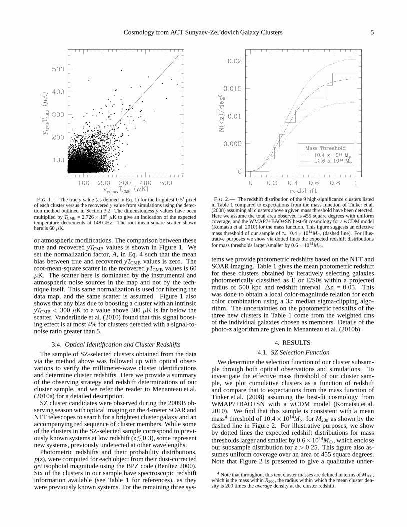
FIG. 1.— The truey value (as defined in Eq. 1) for the brightest 0.5′ pixelof each cluster versus the recoveredy value from simulations using the detec-tion method outlined in Section 3.2. The dimensionlessy values have beenmultiplied byTCMB = 2.726× 106

µK to give an indication of the expectedtemperature decrements at 148 GHz. The root-mean-square scatter shownhere is 60µK.

or atmospheric modifications. The comparison between thesetrue and recoveredyTCMB values is shown in Figure 1. Weset the normalization factor,A, in Eq. 4 such that the meanbias between true and recoveredyTCMB values is zero. Theroot-mean-square scatter in the recoveredyTCMB values is 60µK. The scatter here is dominated by the instrumental andatmospheric noise sources in the map and not by the tech-nique itself. This same normalization is used for filtering thedata map, and the same scatter is assumed. Figure 1 alsoshows that any bias due to boosting a cluster with an intrinsicyTCMB < 300µK to a value above 300µK is far below thescatter. Vanderlinde et al. (2010) found that this signal boost-ing effect is at most 4% for clusters detected with a signal-to-noise ratio greater than 5.

3.4. Optical Identification and Cluster Redshifts

The sample of SZ-selected clusters obtained from the datavia the method above was followed up with optical obser-vations to verify the millimeter-wave cluster identificationsand determine cluster redshifts. Here we provide a summaryof the observing strategy and redshift determinations of ourcluster sample, and we refer the reader to Menanteau et al.(2010a) for a detailed description.

SZ cluster candidates were observed during the 2009B ob-serving season with optical imaging on the 4-meter SOAR andNTT telescopes to search for a brightest cluster galaxy and anaccompanying red sequence of cluster members. While someof the clusters in the SZ-selected sample correspond to previ-ously known systems at low redshift (z<∼0.3), some representnew systems, previously undetected at other wavelengths.

Photometric redshifts and their probability distributions,p(z), were computed for each object from their dust-correctedgri isophotal magnitude using the BPZ code (Benítez 2000).Six of the clusters in our sample have spectroscopic redshiftinformation available (see Table 1 for references), as theywere previously known systems. For the remaining three sys-

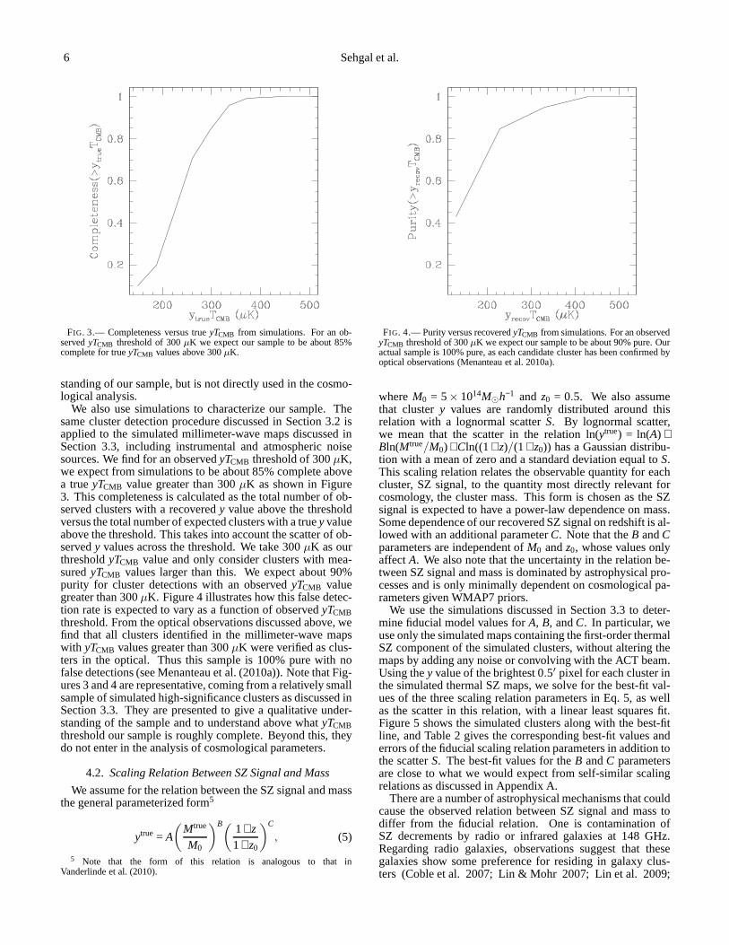
FIG. 2.— The redshift distribution of the 9 high-significance clusters listedin Table 1 compared to expectations from the mass function ofTinker et al.(2008) assuming all clusters above a given mass threshold have been detected.Here we assume the total area observed is 455 square degrees with uniformcoverage, and the WMAP7+BAO+SN best-fit cosmology for a wCDMmodel(Komatsu et al. 2010) for the mass function. This figure suggests an effectivemass threshold of our sample of≈ 10.4× 1014M⊙ (dashed line). For illus-trative purposes we show via dotted lines the expected redshift distributionsfor mass thresholds larger/smaller by 0.6×1014M⊙.

tems we provide photometric redshifts based on the NTT andSOAR imaging. Table 1 gives the mean photometric redshiftfor these clusters obtained by iteratively selecting galaxiesphotometrically classified as E or E/S0s within a projectedradius of 500 kpc and redshift interval|∆z| = 0.05. Thiswas done to obtain a local color-magnitude relation for eachcolor combination using a 3σ median sigma-clipping algo-rithm. The uncertainties on the photometric redshifts of thethree new clusters in Table 1 come from the weighted rmsof the individual galaxies chosen as members. Details of thephoto-z algorithm are given in Menanteau et al. (2010b).

4. RESULTS

4.1. SZ Selection Function

We determine the selection function of our cluster subsam-ple through both optical observations and simulations. Toinvestigate the effective mass threshold of our cluster sam-ple, we plot cumulative clusters as a function of redshiftand compare that to expectations from the mass function ofTinker et al. (2008) assuming the best-fit cosmology fromWMAP7+BAO+SN with a wCDM model (Komatsu et al.2010). We find that this sample is consistent with a meanmass4 threshold of 10.4×1014M⊙ for M200 as shown by thedashed line in Figure 2. For illustrative purposes, we showby dotted lines the expected redshift distributions for massthresholds larger and smaller by 0.6×1014M⊙, which encloseour subsample distribution forz> 0.25. This figure also as-sumes uniform coverage over an area of 455 square degrees.Note that Figure 2 is presented to give a qualitative under-

4 Note that throughout this text cluster masses are defined in terms ofM200,which is the mass withinR200, the radius within which the mean cluster den-sity is 200 times theaveragedensity at the cluster redshift.

6 Sehgal et al.

FIG. 3.— Completeness versus trueyTCMB from simulations. For an ob-servedyTCMB threshold of 300µK we expect our sample to be about 85%complete for trueyTCMB values above 300µK.

standing of our sample, but is not directly used in the cosmo-logical analysis.

We also use simulations to characterize our sample. Thesame cluster detection procedure discussed in Section 3.2 isapplied to the simulated millimeter-wave maps discussed inSection 3.3, including instrumental and atmospheric noisesources. We find for an observedyTCMB threshold of 300µK,we expect from simulations to be about 85% complete abovea trueyTCMB value greater than 300µK as shown in Figure3. This completeness is calculated as the total number of ob-served clusters with a recoveredy value above the thresholdversus the total number of expected clusters with a trueyvalueabove the threshold. This takes into account the scatter of ob-servedy values across the threshold. We take 300µK as ourthresholdyTCMB value and only consider clusters with mea-suredyTCMB values larger than this. We expect about 90%purity for cluster detections with an observedyTCMB valuegreater than 300µK. Figure 4 illustrates how this false detec-tion rate is expected to vary as a function of observedyTCMBthreshold. From the optical observations discussed above,wefind that all clusters identified in the millimeter-wave mapswith yTCMB values greater than 300µK were verified as clus-ters in the optical. Thus this sample is 100% pure with nofalse detections (see Menanteau et al. (2010a)). Note that Fig-ures 3 and 4 are representative, coming from a relatively smallsample of simulated high-significance clusters as discussed inSection 3.3. They are presented to give a qualitative under-standing of the sample and to understand above whatyTCMBthreshold our sample is roughly complete. Beyond this, theydo not enter in the analysis of cosmological parameters.

4.2. Scaling Relation Between SZ Signal and Mass

We assume for the relation between the SZ signal and massthe general parameterized form5

ytrue = A

(

Mtrue

M0

)B( 1+ z1+ z0

)C

, (5)

5 Note that the form of this relation is analogous to that inVanderlinde et al. (2010).

FIG. 4.— Purity versus recoveredyTCMB from simulations. For an observedyTCMB threshold of 300µK we expect our sample to be about 90% pure. Ouractual sample is 100% pure, as each candidate cluster has been confirmed byoptical observations (Menanteau et al. 2010a).

whereM0 = 5× 1014M⊙h−1 and z0 = 0.5. We also assumethat clustery values are randomly distributed around thisrelation with a lognormal scatterS. By lognormal scatter,we mean that the scatter in the relation ln(ytrue) = ln(A) +Bln(Mtrue/M0) +Cln((1+ z)/(1+ z0)) has a Gaussian distribu-tion with a mean of zero and a standard deviation equal toS.This scaling relation relates the observable quantity for eachcluster, SZ signal, to the quantity most directly relevant forcosmology, the cluster mass. This form is chosen as the SZsignal is expected to have a power-law dependence on mass.Some dependence of our recovered SZ signal on redshift is al-lowed with an additional parameterC. Note that theB andCparameters are independent ofM0 andz0, whose values onlyaffectA. We also note that the uncertainty in the relation be-tween SZ signal and mass is dominated by astrophysical pro-cesses and is only minimally dependent on cosmological pa-rameters given WMAP7 priors.

We use the simulations discussed in Section 3.3 to deter-mine fiducial model values forA, B, andC. In particular, weuse only the simulated maps containing the first-order thermalSZ component of the simulated clusters, without altering themaps by adding any noise or convolving with the ACT beam.Using they value of the brightest 0.5′ pixel for each cluster inthe simulated thermal SZ maps, we solve for the best-fit val-ues of the three scaling relation parameters in Eq. 5, as wellas the scatter in this relation, with a linear least squares fit.Figure 5 shows the simulated clusters along with the best-fitline, and Table 2 gives the corresponding best-fit values anderrors of the fiducial scaling relation parameters in addition tothe scatterS. The best-fit values for theB andC parametersare close to what we would expect from self-similar scalingrelations as discussed in Appendix A.

There are a number of astrophysical mechanisms that couldcause the observed relation between SZ signal and mass todiffer from the fiducial relation. One is contamination ofSZ decrements by radio or infrared galaxies at 148 GHz.Regarding radio galaxies, observations suggest that thesegalaxies show some preference for residing in galaxy clus-ters (Coble et al. 2007; Lin & Mohr 2007; Lin et al. 2009;

Cosmology from ACT Sunyaev-Zel’dovich Galaxy Clusters 7

æ

æ

æ

æ

æ

æ

æ

æ

æ

æ

æ

æ

æ

æ

æ

æ

æ

æ

æ

æ

æ

æ

æ

æ

æ

æ

æ

æ

æ

æ

æ

æ æ

æ

æ

æ

æ

æ

æ

æ

æ

æ

æ

æ

æ

æ

æ

æ

æ

æ

æ

æ

æ

æ

æ

æ

æ

æ

æ

æ

æ

æ æ

æ

æ

æ

æ

æ

æ

æ

æ

æ

æ

æ

æ æ

æ

æ

æ

æ

æ

æ

æ

æ

æ

æ

æ

æ

æ

æ

æ

æ

æ

æ

æ

æ

æ

æ

æ

æ

æ

æ

æ

æ

æ

æ

æ

æ

æ

æ

æ

æ

æ

æ

æ

æ

æ

æ

æ

æ

æ

æ

ææ

ææ

æ

æææ

æ

æ

æ

æ

æ

æ

æ

æ

æ

æ

æ

æ

æ

æ

æ

æ

æ

æ

æ

æ

æ

æ

æ

æ

æ

ææ

æ æ

æ

æ

æ

æ

æ

æ

æ

æ

æ

æ

æ

æ

æ

æ

æ

æ

æ

æ

ææ

æ

æ

ææ

æ

æ

æ

æ

æ

æ

æ

æ

æ

æ

æ

æ

æ

æ

æ

æ

æ

æ

æ

æ

æ

æ

æ

æ

æ

æ

æ

æ

æ

æ

æ

æ

æ

æ

æ

æ

æ

æ

æ

æ

æ

æ

æ

æ

æ

æ

æ

æ

æ

æ

æ

æ

æ

æ

æ

æ

æ

æ

æ

æ

æ

æ

æ

æ

æ

æ

ææ

æ

æ

æ

æ

æ

æ

æ

ææ

æ

æ

æ

æ

æ

æ

æ

ææ

æ

æ

æ

æ

æ

æ

æ

æ

æ

æ

ææ

æ

æ

æ

æ

æ

æ

æ

æ

æ

æ

ææ

æ

æ

æ

æ

æ

æ

æ

æ

æ

æ

æ

æ æ

æ

æ

æ

æ

æ

æ

æ

æ

æ

æ

æ

æ

æ

æ

æ

æ

æ

æ

æ

æ

æ

æ

æ

æ

æ

æ

æ

æ

æ

æ

æ

æ

æ

æ

æ

æ

æ

æ

æ

æ

æ

æ

æ

æ

æ

æ

æ

æ

æ

æ

æ

æ

æ

æ

æ

æ

æ

æ

æ

æ

æ

æ

æ

æ

æ

æ æ

æ

æ

æ

æ

æ

æ

æ

æ

æ

æ

æ

æ

æ

æ

æ

æ

æ

æ

æ

æ

æ

æ

ææ

æ

æ

æ

æ

æ

æ

æ

æ

æ

æ

æ

æ

æ

æ

æ

ææ

æ

æ

æ

æ

æ

æ

æ

æ

æ

æ

æ

æ

æ

æ

æ

æ

æ

æ

æ

æ

æ

æ

ææ

ææ

æ

æ

æ

æ

æ

æ

æ

æ

æ

ææ

æ

æ

æ

æ

æ

æ

æ

æ

æ

æ

æ

æ

æ

æ

æ

æ

æ

æ

æ

æ

æ

æ

æ

æ

æ æ

æ

æ

æ

æ

æ

æ

æ

æ

æ

æ

æ

æ

ææ

æ

æ

æ

æ

æ

æ

æ

æ

æ

æ

æ

æ

æ

æ

æ

æ

æ

æ

æ

æ

æ

æ

æ

æ

æ

æ

æ

æ

æ

ææ

æ

æ

æ

ææ

æ

æ

æ

æ

æ

æ

æ

æ

æ

æ

æ

æ

æ

æ

æ

æ

æ

æ

æ

æ

æ

æ

æ

æ

æ

ææ

æ

æ

æ

æ

æ

ææ

æ

æ

æ

æ

æ

æ

æ

æ

æ

æ

æ

æ

æ

æ

ææ

æ

æ

æ

æ

æ

æ

æ

æ

ææ

æ

æ

æ

æ

æ

æ

æ

æ

ææ

æ

æ

æ

æ

æ

æ

æ

æ

æ

æ

æ

æ

æææ

æ

æ

æ

æ

æ

æ

æ

æ

æ

æ

æ

æ

æ

æ

æ

ææ

æ

æ

æ

æ

æ

æ

æ

æ

æ

æ

æ

æ

æ

æ

æ

æ

æ

ææ

æ

æ

æ

æ

æ

æ

æ

æ

æ

æ

æ

ææ

æ

æ

æ

æ

æ

æ

æ

æ

æ

æ

æ

æ

æ

æ

æ

æ

æ

æ

æ

æ

ææ

æ

æ

æ

æ

æ

æ

æ

æ

æ

æ

æ

æ

æ

æ

æ

æ

æ

æ

æ

æ

æ

æ

æ

ææ

æ

æ

æ

æ

æ

æ

æ

æ

æ

æ

ææ

æ

æ

æ

æ

æ

æ

æ

æ

æ

æ

æ

æ

æ

ææ

æ

æ

æ

æ

æ

æ

æ

æ

æ

æ

æ

æ

æ

æ

æ

æ

æ

æ

æ

æ

æ

æ

æ

æ æ

æ

æ

æ

æ

ææ

æ

æ

æ

æ

æ

æ

æ

æ

æ

æ

æ

æ

æ

æ

æ

æ

ææ

æ

æ

æ

æ

æææ

æ

æ

æ

æ

æ

æ

æ

æ

æ

æ

æ

æ

æ

æ

æ

æ

æ

æ

æ

æ

æ

æ

æ

æ

æ

æ

æ

æ

æ

æ

æ

æ

æ

æ

æ

æ

æ

æ

æ

æ

æ

ææ

æ

æ

æ

æ

æ

æ

ææ

æ

æ

æ

æ

æ

æ

æ

æ

ææ

æ

æ

æ

æ

æ

æ

æ

æ

æ

æ

æ

æ

ææ

æ

æ

æ

æ

ææ

æ

æ

æ

æ

æ

æ

æ

æ

æ

æ

æ

æ

æ

æ

æ

ææ

æ

æ

æ

æ

æ

æ

æ

æ

æ

æ

æ

æ

æ

æ

æ

æ

æ

ææ

ææ

æ

æ

æ

æ

ææ

æ

æ

æ

æ

æ

æ

æ

æ

ææ

æ

æ

æ

æ

æ

æ

æ

æ

æ

æ

æ

æ

æ

æ

æ

æ

æ

æ

æ

æ

æ

æ

æ

æ

æ

æ

æ

æ

æ

æ

æ

æ

æ

æ

æ

æ

æ

æ

æ

æ

æ

æ

ææ

æ

æ

æ

æ

æ

æ

ææ

æ

æ

æ

æ

æ

æ

æ æ

æ

ææ

æ

æ

æ

æ

æ

æ

æ

æ

æ

ææ

æ

æ

æ

æ

æ

æ

æ

æ

æ

æ

æ

æ

æ

æ

æ

ææ

æ

æ

æ

æ

æ

æ

æ

æ

æ

æ

æ

æ

æ

æ

æ

æ

æ

æ

æ

æ

æ

æ

æ

æ

æ

æ

æ

æ

æ

æ

æ

æ

æ

æ

æ

æ

æ

æ æ æ

æ

æ

æ

æ

æ

æ

æ

æ

æ

æ

æ

æ

æ

æ

æ

æ

æ

æ

æ

æ

æ

æ

æ

æ

æ

æ

æ

æ

æ

æ

æ

æ

æ

æ

æ

æ

æ

ææ

æ

æ

ææ

æ

æ

ææ

æ

æ

æ

æ

æ

æ

æ

æ

æ

æ

æ

æ

æ

æ

æ

æ

æ

æ

æ æ

æ

æ

æ

æ

æ

æ

æ

æ

ææ

æ

æ

æ

æ

æ

æ

æ

æ

æ

æ

æ

æ

æ

æ

æ

æ

æ

æ

3 5 10 15 20 30

210-5

510-5

110-4

210-4

M200 H1014 M

h-1L

y tru

eHH

1+zL1

.5LC

FIG. 5.— Relation between truey and the cluster mass from simulations,including clusters withM200 > 3× 1014M⊙h−1 andz> 0.15. The best-fitscaling relation parameters in Eq. 5 are found with a least-squares fit, andthe resulting best-fit surface is plotted in two-dimensionsas the solid lineabove. The lognormal scatter between the trueyvalues and the best-fit scalingrelation is 26%.

Mandelbaum et al. 2009). However, using a model of ra-dio galaxies that describes their correlation with halos, theamount of contamination expected from radio galaxies wasfound to be negligible for (Sehgal et al. 2010). For redshifts< 1, star formation, which is responsible for infrared galaxyemission, is expected to be quenched in high-density environ-ments. At low redshifts (z∼ 0.06) the fraction of all galaxiesthat are star forming galaxies is∼ 16% in clusters (Bai et al.2010). While this percentage is expected to increase at higherredshifts, given that the total infrared background at 150 GHzis roughly 30µK (Fixsen et al. 1998), it is unlikely that in-frared galaxy contamination could be significant for clusterswith yTCMB > 300µK. Lima et al. (2010) have also shownthat the lensing of infrared galaxies by massive clusters shouldnot introduce a significant bias in the measured SZ signals.

Another way for the observed SZ signal to be lower thanthe fiducial model is if clusters have a significant amount ofnonthermal pressure. This pressure would not be observedas part of the SZ signal, however, it would play an importantrole in counteracting the gravitational pressure from the clus-ter mass. Such nonthermal pressure can take the form of smallscale turbulence, bulk flows, or cosmic rays. Simulationsand observations suggest contributions to the total pressurefrom cosmic rays to be about 5− 10% (Jubelgas et al. 2008;Pfrommer & Enßlin 2004) and from turbulent pressure to bebetween 5− 20% (Lau et al. 2009; Meneghetti et al. 2010;Burns et al. 2010), with only the latter work suggesting levelsas high as 20% and that largely at the cluster outskirts. Theseprocesses have a much larger impact on lower mass clus-ters and groups where the gravitational potential is not strongenough to tightly bind the cluster gas (e.g., Battaglia et al.2010; Shaw et al. 2010; Trac et al. 2010). However, for themassive systems considered here, this again is not expectedtobe a significant issue. One astrophysical process that can havea significant affect on the clustery values is major mergers.We certainly have at least one in our sample (Bullet cluster),but note the extreme rarity of such objects in general.

4.3. Cluster Likelihood Function

In order to constrain cosmological parameters with ourcluster sample, we construct a likelihood function specificforclusters, and we map out the posterior distribution to findmarginalized distributions for each parameter. We followCash (1979) who derived the likelihood function in the caseof Poisson statistics giving

lnL = lnPr(ni|λi) =Nb∑

i=1

(ni lnλi −λi). (6)

Pr is the probability of measuringni given modeled countsλi. HereNb is the total number of observed bins in SZ sig-nal - redshift space, andλi is the modeled number of clustersin the ith bin. We also take the bin sizes to be small enoughso that no more than one observed cluster is in each bin. Themodeled cluster count,λi , is a function of the SZ signal andredshift of the given bin (which we callyobs andzobs) as wellas the set of cosmological parameters,c j. The modeledcount is also a function of the parameters of the SZ signal -mass scaling relation (A,B,C,S) given in Eq. 5, since it is theabundance of clusters as a function of mass that is tied to cos-mology via the mass function. For this work we use the massfunction given in Tinker et al. (2008). A derivation of the fullcluster likelihood function used in this analysis can be foundin Appendix B. This likelihood is given by Eq. B8 and is afunction of the parametersc j andA,B,C,S.

We assume normal errors of 2.2×10−5 onyobs (correspond-ing to an error inyTCMB of 60µK) and 0.1 onzobs. We take 0.1as the redshift uncertainty for convenience even though sixofour clusters have spectroscopic redshifts. However, the red-shift error does not dominate the uncertainty of our results.We also assume Gaussian priors onA,B,C, and S centeredaround the fiducial values given in Table 2, with conservative1σ uncertainties of 35%,20%,50%, and 20% respectively ofthe fiducial values. These priors were determined by find-ing the relation between SZ signal and mass from simulatedthermal SZ maps with varying gas models. In particular, weuse two simulated thermal SZ maps analogous to those dis-cussed in Section 4.2, with the gas physics models in thesemaps based on the adiabatic and the nonthermal20 models de-scribed in Trac et al. (2010). The adiabatic model assumes nofeedback, star-formation, or other nonthermal processes thatcould lower the SZ signal as a function of mass. The nonther-mal20 model assumes more star-formation than the fiducialmodel and 20% nonthermal pressure support for all clustersat all radii, which is a larger amount of nonthermal pressurethan generally suggested by X-ray observations and hydro-dynamic simulations (e.g., Lau et al. 2009; Meneghetti et al.2010; Burns et al. 2010). These two models span the rangeof plausible gas models for massive clusters given current ob-servations, and the 1σ priors on the scaling relation parame-ters given above are generous given the range in parametersspanned by these models.

4.4. Parameter Constraints

The likelihood function described above was made into astandalone code module which was then interfaced with theMarkov chain software package CosmoMC (Lewis & Bridle2002). Using CosmoMC, we run full chains for the WMAP7data alone (Larson et al. 2010) and for the WMAP7 data plus

8 Sehgal et al.

σ8

w

0.4 0.6 0.8 1 1.2−2.5

−2

−1.5

−1

−0.5

0

σ8

w

0.4 0.6 0.8 1 1.2−2.5

−2

−1.5

−1

−0.5

0

FIG. 6.— Likelihood contour plots ofw versusσ8 showing 1σ and 2σ marginalized contours.Left: Blue contours are for WMAP7 alone, and red contours arefor WMAP7 plus ACT SZ detected clusters, fixing the mass-observable relation to the fiducial relation given in Section 4.2. Right: Contours are the same as inthe left panel, except that the uncertainty in the mass-observable relation has been marginalized over within priors discussed in Section 4.3.

TABLE 2BEST-FIT SCALING RELATION PARAMETERS

Model and Data Set A B C S

Simulation Fiducial Values (5.67±0.05)×10−5 1.05±0.03 1.29±0.05 0.26wCDM WMAP7 + ACT Clusters (8.77±3.77)×10−5 1.75±0.28 0.97±0.68 0.27±0.13

TABLE 3COSMOLOGICAL PARAMETER CONSTRAINTS FORσ8 AND w

Model and Data Set σ8 w

wCDM WMAP7+BAO+SN 0.802±0.038 −0.98±0.053wCDM WMAP7 0.835±0.139 −1.11±0.40

wCDM WMAP7 + ACT Clusters (fiducial scaling relation) 0.821±0.044 −1.05±0.20wCDM WMAP7 + ACT Clusters (marginalized over scaling relation) 0.851±0.115 −1.14±0.35

our ACT cluster subsample. We assume a wCDM cosmo-logical model which allowsw to be a constant not equal to−1, assumes spatial flatness, and which has as free parame-ters:Ωbh2, Ωch2, θ∗, τ , w, ns, ln[1010As], andASZ as definedin Larson et al. (2010). The parameterσ8 is derived fromthe first seven of these parameters and is kept untied toASZas the link between the two is in part what we are investi-gating. We run the WMAP7 plus ACT clusters chain undertwo cases: one where the values ofA,B,C, andS are fixedto the fiducial values given in Section 4.2 and listed in Table2, and one whereA,B,C, and S are allowed to vary withinthe conservative priors given in Section 4.3. For the lattercase, we add these four new parameters to the CosmoMCcode. At each step of the chain, CosmoMC calls the soft-ware package CAMB6 to generate both the microwave back-ground power spectrum and matter power spectrum as a func-tion of the input cosmology, and then the natural logarithmsof both the WMAP and cluster likelihoods are added. Wedetermine the posterior probability density function throughthe Markov chain process and use a simple R−1 statistic(Gelman & Rubin 1992) of R−1 < 0.01 to check for conver-

6 www.camb.info

gence of the chains.The best-fit marginalized 1σ and 2σ contours, obtained

from this process, are shown in Figure 6 forw and σ8.The blue contours show the constraints for WMAP7 alone,while the red contours show the constraints from the unionof WMAP7 plus our ACT cluster subsample. The left panelshows the best-fit contours with the SZ signal - mass scalingrelation fixed to the fiducial relation obtained from the sim-ulations. The right panels show the constraints allowing thefour parameters of the scaling relation to vary. Table 3 lists thebest-fit parameter values forσ8 andw with their 1σ marginal-ized uncertainties. Table 2 lists the best-fit scaling relationvalues and 1σ uncertainties as well as the fiducial values ob-tained from simulations as discussed in Section 4.2 for com-parison. We note that for the remaining seven parameters fitin the analyses combining WMAP7 plus ACT clusters (Ωbh2,Ωch2, θ∗, τ , ns, ln[1010As], andASZ), we find best-fit valuesconsistent with the best-fit values from WMAP7 alone with amodest improvement in the marginalized errors.

4.5. Stacked SZ Signal

We also perform a stacking analysis of the nine clusterslisted in Table 1 to measure average cluster SZ profiles, which

Cosmology from ACT Sunyaev-Zel’dovich Galaxy Clusters 9

FIG. 7.— Average profile from stacking the 9 clusters presented in Table1 (black solid line) compared with the average profile stacking 40 clusterswith unsmoothedyTCMB values greater than 300µK in simulated thermal SZmaps convolved with the ACT beam (dashed blue line). The dashed blue lineshows the average profile for clusters simulated with the fiducial SZ model,while the dotted red (bottom) and dot-dashed green (top) lines show the sameassuming the adiabatic and nonthermal20 SZ models respectively which arediscussed in Section 4.3. For the profiles of the 9 clusters inthe data, weremoved a mean background level from the profile of each cluster. Error barsfor the simulated clusters have been offset by 0.1′ for clarity, and are smallerthan those from the data. Error bars for the adiabatic and nonthermal20 mod-els are not shown, but are of similar size as for the fiducial model.

can be compared with simulations. We stack the 9 clusters inthe data map prior to any filtering, after subtracting a meanbackground level for each cluster profile using an annulus 15′

from the center of each cluster and 0.5′ wide. The stacked av-erage profile is given by the solid black line in Figure 7. Thesame procedure is preformed on all simulated clusters withunsmoothedyTCMB values greater than 300µK in simulatedthermal SZ maps. There are 40 of these simulated clustersin total over 6 different 455 square degree maps spanning thesame redshift range as the data. These simulated clusters arestacked in thermal SZ maps convolved with the ACT beamto mimic the data, and their average profile is given by thedashed blue line in Figure 7. Error bars represent the standarddeviation of the mean in each radial bin. The blue dashed linerepresents the stacked profiles of simulated clusters assumingthe fiducial SZ model. The red dotted and green dot-dashedlines show the stacked profiles of simulated clusters assum-ing the adiabatic and nonthermal20 SZ models discussed inSection 4.3. The error bars have not been included for the lat-ter two models in Figure 7, but they are of similar size as forthe fiducial model. We find good agreement in the averageprofiles of the clusters in the data and simulated with the fidu-cial model as shown in Figure 7, which suggests that there isno significant misestimate of the SZ signal for these massivesystems.

5. DISCUSSION

From Table 3 we see overall agreement betweenσ8 andwas measured with only WMAP7 and as measured with thehigh-significance ACT cluster sample plus WMAP7. We findσ8 = 0.821± 0.044 andw = −1.05± 0.20 if we assume the

fiducial scaling relation, a decrease in the uncertainties onthese parameters by roughly a factor of three and two re-spectively as compared to WMAP7 alone. This indicatesthe potential statistical power associated with cluster mea-surements. Marginalizing over the uncertainty in this scalingrelation, we findσ8 = 0.851± 0.115 andw = −1.14± 0.35,an uncertainty comparable to that of WMAP7 alone. Wealso see consistency when comparing these constraints to thebest-fit constraints from WMAP7 plus baryon acoustic oscil-lations plus type Ia supernovae, which giveσ8 = 0.802±0.038and w = −0.980± 0.053 for a wCDM cosmological model(Komatsu et al. 2010). As the latter are all expansion rateprobes, this suggests agreement between expansion rate andgrowth of structure measures. Both also showw is consistentwith −1, giving further support to dark energy being an energyof the vacuum.

These results are also consistent with analyses from X-raycluster samples givingσ8(Ωm/0.25)0.47 = 0.813±0.013 (stat)±0.024 (sys) andw = −1.14± 0.21 (Vikhlinin et al. 2009),Ωm = 0.23± 0.04, σ8 = 0.82± 0.05, andw = −1.01± 0.20for a wCDM model (Mantz et al. 2010), andΩm = 0.30+0.03

−0.02,σ8 = 0.85+0.04

−0.02 from WMAP5 plus X-ray clusters (Henry et al.2009) . We also find consistency with optical samples yield-ing σ8(Ωm/0.25)0.41 = 0.832±0.033 for a flatΛCDM model(Rozo et al. 2010). Vanderlinde et al. (2010) findσ8 = 0.804±0.092 andw = −1.049±0.291 for a wCDM model using SZclusters detected by SPT plus WMAP7.

This analysis also suggests consistency between the fiducialmodel of cluster astrophysics used here to describe massiveclusters and the data. Table 3 shows agreement in best-fit cos-mological parameters between growth rate and expansion rateprobes when we hold fixed our fiducial relation between SZsignal and mass. When we allow the scaling relation parame-ters to be free, we find best-fit values that are broadly consis-tent with those of our fiducial relation. We note that while the1σ range of theB parameter is higher than the fiducial value,the fiducial value is enclosed by the 2σ range of 1.75+0.4

−0.7. Thehigher value of theB parameter may indicate some curvaturein the true scaling relation away from the fiducial model atthe high-mass end. This may also be suggested by Figure 5where the simulated clusters seem to prefer highery valuesthan the fiducial relation would suggest for the most massivesystems. The agreement between cosmological parametersfrom expansion rate and growth of structure probes when fix-ing the SZ signal - mass scaling relation to the fiducial modeland the broad agreement between fiducial and best-fit scal-ing relation parameters when the latter are allowed to be free,suggest our data is broadly consistent with expectations forthe SZ signal of massive clusters. This is also suggested bycomparing the stacked SZ detected clusters in the data withsimulations as shown in Figure 7.

We would expect the above to be the case as massive clus-ters have been studied far better than lower mass clusters witha variety of multi-wavelength observations. In addition, anumber of astrophysical processes that are not perfectly un-derstood, such as nonthermal processes and point source con-tamination, affect the gas physics of lower mass clusters muchmore than that of the most massive systems. In general, theseprocesses tend to suppress the SZ power spectrum over thatof a straightforward extrapolation based on the most massivesystems. This is an important effect as lower mass systems(< 1014M⊙) contribute as much to the SZ power spectrum atl ∼ 3000 as systems at higher mass (Komatsu & Seljak 2002;

10 Sehgal et al.

Trac et al. 2010). The power spectrum nearl = 3000 has beenrecently measured by and discussed in Lueker et al. (2010),Das et al. (2010) and Dunkley et al. (2010).

There are a number of ways the cosmological constraintspresented here could be further improved. Clearly the largestuncertainty is the relation between SZ signal and mass, andfurther X-ray observations of massive clusters, particularly athigher redshifts where X-ray observations have been limited,would help to calibrate this relation. Further targeted observa-tions of massive clusters at millimeter-wave frequencies withenough resolution and sensitivity to identify point sourceswould offer a better handle on contamination levels. In addi-tion, an analysis using multiple frequency bands, which wouldemploy the spectral information of the SZ signal, may behelpful in determining cluster sizes and measuring integratedYs. This could help reduce the scatter in the relation betweenSZ signal and mass. Spectroscopic redshifts of all the clustersin a given SZ sample would also help to reduce uncertaintyon the cosmological parameters. In addition, millimeter-wavemaps with lower instrument noise, would greatly reduce thescatter between the recovered and true SZ signal. Such mapsare expected with ACTpol (Niemack et al. 2010) and SPTpol(McMahon et al. 2009) coming online in the near future.

With continued SZ surveys such as ACT and SPT andtheir polarization counterparts, in addition to data forthcom-ing from thePlancksatellite, we will no doubt increase thenumber of SZ cluster detections. We anticipate that upcom-ing larger galaxy cluster catalogs will make significant contri-butions to our understanding of both cluster astrophysics andcosmology.

NS would like to thank Phil Marshall for very insightfuldiscussions regarding the construction of the likelihood func-tion and Adam Mantz and David Rapetti for many helpfuldiscussions, particularly in regard to CosmoMC. NS also ac-knowledges useful conversations with Michael Busha, GlennMorris, Jeremy Tinker, and Roberto Trotta.

This work was supported by the U.S. National Sci-ence Foundation through awards AST-0408698 for the

ACT project, and PHY-0355328, AST-0707731 and PIRE-0507768. Funding was also provided by Princeton Universityand the University of Pennsylvania. The PIRE program madepossible exchanges between Chile, South Africa, Spain andthe U.S. that enabled this research program. Computationswere performed on the GPC supercomputer at the SciNetHPC Consortium. SciNet is funded by: the Canada Founda-tion for Innovation under the auspices of Compute Canada;the Government of Ontario; Ontario Research Fund – Re-search Excellence; and the University of Toronto.

NS is supported by the U.S. Department of Energy con-tract to SLAC no. DE-AC3-76SF00515. AH, TM, SD, andVA were supported through NASA grant NNX08AH30G.AH received additional support from a Natural Science andEngineering Research Council of Canada (NSERC) PGS-Dscholarship. AK and BP were partially supported throughNSFAST-0546035 and AST-0606975, respectively, for workon ACT. ES acknowledges support by NSF Physics Fron-tier Center grant PHY-0114422 to the Kavli Institute of Cos-mological Physics. HQ and LI acknowledge partial sup-port from FONDAP Centro de Astrofisica. JD received sup-port from an RCUK Fellowship. KM, MH, and RW re-ceived financial support from the South African National Re-search Foundation (NRF), the Meraka Institute via fundingfor the South African Centre for High Performance Com-puting (CHPC), and the South African Square KilometerArray (SKA) Project. RD was supported by CONICYT,MECESUP, and Fundacion Andes. RH acknowledges fund-ing from the Rhodes Trust. SD acknowledges support fromthe Berkeley Center for Cosmological Physics. YTL ac-knowledges support from the World Premier InternationalResearch Center Initiative, MEXT, Japan. Some of the re-sults in this paper have been derived using the HEALPixpackage (Górski et al. 2005). We acknowledge the use ofthe Legacy Archive for Microwave Background Data Anal-ysis (LAMBDA). Support for LAMBDA is provided by theNASA Office of Space Science. The data will be made pub-lic through LAMBDA (http://lambda.gsfc.nasa.gov/) and theACT website (http://www.physics.princeton.edu/act/).

APPENDIX

A. SELF-SIMILAR SCALING RELATION BETWEEN SZ SIGNAL AND MASS

If clusters were self-similar and isothermal, then we wouldexpect the scaling relation between SZ signal and mass to be

Yhalo∝ M5/3haloE(z)2/3 fgas/d

2A, (A1)

whereYhalo is the Compton y-parameter integrated over the surface of the cluster in units of arcmin2, andE(z) = [Ωm(1+ z)3 +ΩΛ]1/2 for a flatΛCDM cosmology. The angular diameter distance is denoted bydA, and fgas is the gas mass fraction. For theCompton y-parameter integrated over a fixed aperture we have

Yaperture∝Yhalo

(

Raperture

Rhalo

)2

, (A2)

whereRaperture∝ dA andRhalo∝ M1/3haloE(z)−2/3. Note that this equation is appropriate if the aperture sizeis smaller than the size

of the cluster. The above gives

Yaperture∝ MhaloE(z)2 fgas. (A3)

To write Yapertureas a function of (1+ z) we note that at z=0.5 (the mean redshift of our cluster sample) E(z) ∝ (1+ z)0.835 forΩm = 0.27. Thus

Yaperture∝ MBhalo(1+ z)C, (A4)

whereB = 1.0 andC = 1.67.

Cosmology from ACT Sunyaev-Zel’dovich Galaxy Clusters 11

B. CLUSTER LIKELIHOOD FUNCTION

Below we describe the construction of the likelihood function for SZ clusters detected in millimeter-wave surveys. FromPoisson statistics, the probability of observingni counts expectingλi counts is

Pr (ni|λi) =λni

i e−λi

ni !. (B1)

Given a data set ofni counts inNb observed bins and a corresponding prediction,λi, the probability of the data given theprediction is

Pr (ni|λi) =Nb∏

i=1

λnii e−λi

ni !, (B2)

whereλi = Pr (yobs,zobs,A,B,C,S,c j)N∆yobs∆zobs. HerePr(yobs,zobs,A,B,C,S,c j) is the probability of observing a cluster in

bin i, andN is a normalization factor givingλi units of counts (see below). The observed SZ signal and redshift of a given clusterare denoted byyobs andzobs, and∆yobs and∆zobs denote the size of the bin. The parametersA,B,C,Sdescribe the scaling relationbetween SZ signal and mass and are defined below. The cosmological parameters are indicated byc j.

If we allow the bin sizes to be small enough that each observedbin holds no more than one observed cluster, then

lnPr (ni|λi) =n

∑

i=1

lnλi −Nb∑

i=1

λi = lnL (B3)

as given in Cash (1979). Note that the ln(ni!) term has been dropped as it is independent of any change in parameters, andnrepresents the total number of clusters observed. Thus we have

lnL =n

∑

i=1

ln(Pr(yobs,zobs,A,B,C,S,c j)Ndyobsdzobs) −

∫

zobs

∫

yobs

Pr(yobs,zobs,A,B,C,S,c j)Ndyobsdzobs (B4)

with

Pr (yobs,zobs,A,B,C,S,c j) =∫∫∫

Pr(yobs,zobs,A,B,C,S,c j,ytrue,ztrue, lnMtrue)dytruedztruedlnMtrue (B5)

=∫∫∫

Pr(yobs,zobs|A,B,C,S,c j,ytrue,ztrue, lnMtrue)Pr (A,B,C,S,c j,ytrue,ztrue, lnMtrue)dytruedztruedlnMtrue (B6)

=∫∫∫

Pr(yobs,zobs|ytrue,ztrue)Pr(y

true|A,B,C,S,c j,ztrue, lnMtrue)Pr(A,B,C,S,c j,ztrue, lnMtrue)dytruedztruedlnMtrue (B7)

=∫ ∞

−∞dlnMtrue

∫ ∞

0dytrue

∫ ∞

0dztruePr (yobs|ytrue)Pr (zobs|ztrue)Pr(ytrue|A,B,C,S,ztrue, lnMtrue)Pr(lnMtrue,ztrue|c j)

× Pr (c j)Pr(A)Pr(B)Pr(C)Pr(S) (B8)

using the definition of conditional probability. HerePr(c j) is any external prior onc j such as a WMAP prior.We assume the following SZ signal - mass scaling relation with log normal scatter,S,

ytrue = A

(

Mtrue

M0

)B( 1+ z1+ z0

)C

, (B9)

whereM0 = 5×1014M⊙h−1 andz0 = 0.5. This gives

Pr (ytrue|A,B,C,S,ztrue, lnMtrue) =1√

2πSytrueexp

(

−(lnytrue− BlnMtrue−Cln(1+ ztrue) − lnA+ BlnM0 +Cln(1+ z0))2

2S2

)

. (B10)

We also assume Gaussian priors on the scaling relation parameters as indicated by simulations, giving

Pr(A) =1√

2πσAexp

(

−(A− A0)2

2σ2A

)

. (B11)

Similar relations hold forPr(B), Pr(C), andPr(S).From the mass function we have

12 Sehgal et al.

Pr(lnMtrue,ztrue|c j) =dn(lnMtrue,ztrue,c j)

dlnMtrue

dV(ztrue,c j)dztrue

1N, (B12)

where heren is the number density of clusters.N is the total number of clusters when the above mass function is integrated overdlnMtrue anddztrue.

We also assume for the uncertainty on the observed SZ signal and redshift that

Pr(yobs|ytrue) =

1√2πσobs

exp

(

−(yobs− ytrue)2

2σ2obs

)

(B13)

Pr (zobs|ztrue) =

1√2πσz

exp

(

−(zobs− ztrue)2

2σ2z

)

(B14)

where these two expressions should also be multiplied by 21+erf(xtrue/

√2σx)

since the limits of integration are from 0 to∞.

REFERENCES

Arnaud, M., Pratt, G. W., Piffaretti, R., Boehringer, H., Croston, J. H., &Pointecouteau, E. 2009, ArXiv e-prints, 0910.1234

Bahcall, N. A., & Fan, X. 1998, ApJ, 504, 1, arXiv:astro-ph/9803277Bai, L., Rasmussen, J., Mulchaey, J. S., Dariush, A., Raychaudhury, S., &

Ponman, T. J. 2010, ApJ, 713, 637, 1003.0766Battaglia, N., Bond, J. R., Pfrommer, C., Sievers, J. L., & Sijacki, D. 2010,

ArXiv e-prints, 1003.4256Benítez, N. 2000, ApJ, 536, 571Bertin, E., & Arnouts, S. 1996, A&AS, 117, 393Bertschinger, E., & Zukin, P. 2008, Phys. Rev. D, 78, 024015,0801.2431Bode, P., & Ostriker, J. P. 2003, ApJS, 145, 1, arXiv:astro-ph/0302065Bode, P., Ostriker, J. P., & Vikhlinin, A. 2009, ArXiv e-prints, 0905.3748Bode, P., Ostriker, J. P., & Xu, G. 2000, ApJS, 128, 561,

arXiv:astro-ph/9912541Bonaldi, A., Tormen, G., Dolag, K., & Moscardini, L. 2007, MNRAS, 378,

1248, 0704.2535Brodwin, M. et al. 2010, ArXiv e-prints, 1006.5639Brown, M. L. et al. 2009, ApJ, 705, 978, 0906.1003Burns, J. O., Skillman, S. W., & O’Shea, B. W. 2010, ArXiv e-prints,

1004.3553Carlstrom, J. E. et al. 2009, ArXiv e-prints, 0907.4445Cash, W. 1979, ApJ, 228, 939Coble, K. et al. 2007, AJ, 134, 897, arXiv:astro-ph/0608274da Silva, A. C., Kay, S. T., Liddle, A. R., & Thomas, P. A. 2004,MNRAS,

348, 1401, arXiv:astro-ph/0308074Das, S. et al. 2010, ArXiv e-prints, 1009.0847de Grandi, S. et al. 1999, ApJ, 514, 148, arXiv:astro-ph/9902067Dunkley, J. et al. 2010, ArXiv e-prints, 1009.0866Edge, A. C. et al. 1994, A&A, 289, L34, arXiv:astro-ph/9407078Fixsen, D. J., Dwek, E., Mather, J. C., Bennett, C. L., & Shafer, R. A. 1998,

ApJ, 508, 123, arXiv:astro-ph/9803021Fowler, J. W. et al. 2010, ArXiv e-prints, 1001.2934Gelman, A., & Rubin, D. B. 1992, Statist. Sci., 7, 457Górski, K. M., Hivon, E., Banday, A. J., Wandelt, B. D., Hansen, F. K.,

Reinecke, M., & Bartelmann, M. 2005, ApJ, 622, 759,arXiv:astro-ph/0409513

Haehnelt, M. G., & Tegmark, M. 1996, MNRAS, 279, 545,arXiv:astro-ph/9507077

Hall, N. R. et al. 2010, ApJ, 718, 632, 0912.4315Henry, J. P., Evrard, A. E., Hoekstra, H., Babul, A., & Mahdavi, A. 2009,

ApJ, 691, 1307, 0809.3832Herranz, D., Sanz, J. L., Barreiro, R. B., & Martínez-González, E. 2002a,

ApJ, 580, 610, arXiv:astro-ph/0204149Herranz, D., Sanz, J. L., Hobson, M. P., Barreiro, R. B., Diego, J. M.,

Martínez-González, E., & Lasenby, A. N. 2002b, MNRAS, 336, 1057,arXiv:astro-ph/0203486

Hicken, M., Wood-Vasey, W. M., Blondin, S., Challis, P., Jha, S., Kelly,P. L., Rest, A., & Kirshner, R. P. 2009, ApJ, 700, 1097, 0901.4804

Hincks, A. D. et al. 2009, ArXiv e-prints, 0907.0461Infante, L. et al. 2010, in prepJain, B., & Khoury, J. 2010, ArXiv e-prints, 1004.3294Jubelgas, M., Springel, V., Enßlin, T., & Pfrommer, C. 2008,A&A, 481, 33,

arXiv:astro-ph/0603485Kessler, R. et al. 2009, ApJS, 185, 32, 0908.4274Koester, B. P. et al. 2007, ApJ, 660, 239, arXiv:astro-ph/0701265Komatsu, E. et al. 2009, ApJS, 180, 330, 0803.0547Komatsu, E., & Seljak, U. 2002, MNRAS, 336, 1256,

arXiv:astro-ph/0205468Komatsu, E. et al. 2010, ArXiv e-prints, 1001.4538Larson, D. et al. 2010, ArXiv e-prints, 1001.4635Lau, E. T., Kravtsov, A. V., & Nagai, D. 2009, ApJ, 705, 1129, 0903.4895

Lewis, A., & Bridle, S. 2002, Phys. Rev. D, 66, 103511,arXiv:astro-ph/0205436

Lima, M., Jain, B., & Devlin, M. 2010, MNRAS, 406, 2352, 0907.4387Lin, Y., Partridge, B., Pober, J. C., Bouchefry, K. E., Burke, S., Klein, J. N.,

Coish, J. W., & Huffenberger, K. M. 2009, ApJ, 694, 992, 0805.1750Lin, Y.-T., & Mohr, J. J. 2007, ApJS, 170, 71, arXiv:astro-ph/0612521Linder, E. V. 2005, Phys. Rev. D, 72, 043529, arXiv:astro-ph/0507263Lueker, M. et al. 2010, ApJ, 719, 1045, 0912.4317Mandelbaum, R., Li, C., Kauffmann, G., & White, S. D. M. 2009,MNRAS,

393, 377, 0806.4089Mantz, A., Allen, S. W., Rapetti, D., & Ebeling, H. 2010, MNRAS, 1029,

0909.3098Marriage, T. A. et al. 2010a, ApJ submitted——. 2010b, ArXiv e-prints, 1007.5256McMahon, J. J. et al. 2009, in AIP Conference Proceedings on Low

Temperature Detectors, Vol. 1185, 511–514Melin, J.-B., Bartlett, J. G., & Delabrouille, J. 2006, A&A,459, 341,

arXiv:astro-ph/0602424Menanteau, F. et al. 2010a, ArXiv e-prints, 1006.5126——. 2010b, ArXiv e-prints, 1002.2226Meneghetti, M., Rasia, E., Merten, J., Bellagamba, F., Ettori, S., Mazzotta,

P., Dolag, K., & Marri, S. 2010, A&A, 514, A93+, 0912.1343Motl, P. M., Hallman, E. J., Burns, J. O., & Norman, M. L. 2005,ApJ, 623,

L63, arXiv:astro-ph/0502226Murphy, T. et al. 2010, MNRAS, 154, 0911.0002Nagai, D. 2006, ApJ, 650, 538, arXiv:astro-ph/0512208Niemack, M. D. et al. 2010, in Proceedings of SPIE Astronomical

Telescopes and Instrumentation, Vol. 7741, 1006.5049Nozawa, S., Itoh, N., & Kohyama, Y. 1998, ApJ, 508, 17,

arXiv:astro-ph/9804051Percival, W. J. et al. 2010, MNRAS, 401, 2148, 0907.1660Pfrommer, C., & Enßlin, T. A. 2004, A&A, 413, 17Reid, B. A., & Spergel, D. N. 2006, ApJ, 651, 643, arXiv:astro-ph/0601133Riess, A. G. et al. 2009, ApJ, 699, 539, 0905.0695Rozo, E. et al. 2010, ApJ, 708, 645, 0902.3702Schrabback, T. et al. 2010, A&A, 516, A63+, 0911.0053Sehgal, N., Bode, P., Das, S., Hernandez-Monteagudo, C., Huffenberger, K.,

Lin, Y., Ostriker, J. P., & Trac, H. 2010, ApJ, 709, 920, 0908.0540Shapiro, C., Dodelson, S., Hoyle, B., Samushia, L., & Flaugher, B. 2010,

ArXiv e-prints, 1004.4810Shaw, L. D., Nagai, D., Bhattacharya, S., & Lau, E. T. 2010, ArXiv e-prints,

1006.1945Silvestri, A., & Trodden, M. 2009, Reports on Progress in Physics, 72,

096901, 0904.0024Simpson, F., & Peacock, J. A. 2010, Phys. Rev. D, 81, 043512, 0910.3834Sun, M., Voit, G. M., Donahue, M., Jones, C., Forman, W., & Vikhlinin, A.

2009, ApJ, 693, 1142, 0805.2320Sunyaev, R. A., & Zel’dovich, Y. B. 1970, Comments on Astrophysics and

Space Physics, 2, 66——. 1972, Comments on Astrophysics and Space Physics, 4, 173Swetz, D. S. et al. 2010, ArXiv e-prints, 1007.0290Tinker, J., Kravtsov, A. V., Klypin, A., Abazajian, K., Warren, M., Yepes,

G., Gottlöber, S., & Holz, D. E. 2008, ApJ, 688, 709, 0803.2706Trac, H., Bode, P., & Ostriker, J. P. 2010, ArXiv e-prints, 1006.2828Truemper, J. 1990, Sterne und Weltraum, 29, 222Tucker, W. et al. 1998, ApJ, 496, L5+, arXiv:astro-ph/9801120Vanderlinde, K. et al. 2010, ArXiv e-prints, 1003.0003Vikhlinin, A., Kravtsov, A., Forman, W., Jones, C., Markevitch, M., Murray,

S. S., & Van Speybroeck, L. 2006, ApJ, 640, 691, arXiv:astro-ph/0507092Vikhlinin, A. et al. 2009, ApJ, 692, 1060, 0812.2720Werner, N., Churazov, E., Finoguenov, A., Markevitch, M., Burenin, R.,

Kaastra, J. S., & Böhringer, H. 2007, A&A, 474, 707, 0708.3253Zel’dovich, Y. B., & Sunyaev, R. A. 1969, Ap&SS, 4, 301