


Languages
Pages
Legal


1
KTH ROYAL INSTITUTE OF TECHNOLOGY
SINGLE POINT INCREMENTAL FORMING
A study of Forming Parameters, Forming limits and Part accuracy of
Aluminium 2024, 6061 and 7475 alloys
By
Saad Arshad
Thesis Supervisor
Amir Rashid Thesis Examiner
Arne Melander
A thesis submitted to the Department of Industrial Engineering And Production In conformity with the requirements for the degree of Masters of Applied Science
KTH Royal Institute of technology
Stockholm, Sweden
(June, 2012)
Copyright © Saad Arshad, 2012

2
Abstract
Nowadays there is an increasingly demanding need for the development of agile
manufacturing techniques that can easily be adaptable to a constant introduction of new
products in the market. Single point incremental forming (SPIF) is a new innovative and
feasible solution for the rapid prototyping and the manufacturing of small batch sheet parts.
The process is carried out at room temperature (cold forming) and requires a CNC
machining centre, a spherical tip tool and a simple support to fix the sheet being formed.
This work studied the effects of step size, angle, spindle speed, and feed rate on the forming
limits of Aluminium alloys namely AA 2024, AA 6061 and AA 7475 in soft annealed
condition. The Study also includes measuring the strain path and determination of
maximum forming limit angles for the above mentioned alloys. This thesis provides a better
understanding of the influence of rotating tool in the occurrence of fracture without
previous necking or fracture following previous necking.
Surface and geometric accuracy of the parts manufactured was also studied and
comparisons were made between the CAD files and the actual manufactured parts and then
corrections were made accordingly. The main contribution of this thesis to Single stage SPIF
was the successful manufacturing of a Cone shaped parts with almost vertical walls.

3
Acknowledgements
First of all, I would like to thank All Mighty Allah (SWT) for giving me the power to compile
and complete this report.
I would like to express my thankfulness to my Examiner, Professor Arne Melander for his
invaluable scientific advice, discussions and suggestions that provided a stimulating
guidance throughout this work and also for the opportunity that was given to me to develop
my research work at the KTH Royal Institute of Technology.
I am also grateful to my supervisor, Professor Amir Rashid, for his close guidance and his
continuous help and assistance during my research work along with his valuable comments
on my thesis.
Concerning the experimental work performed at the IIP (KTH), I am truly grateful to Lab
manager Jan Stamner for his patience with me and for the opportunity to use the
experimental facilities and for his valuable comments on my thesis and his influence to my
work. I want to also express my special gratitude Dr. Daniel and Dr. Thomas for their
encouragement and support.
I would also like to thank SAAB for providing materials and Mr Mikael Nilsson for many
stimulating discussions.
Deep in my heart, I dedicated this thesis to my parents and Jannet.

4
Table of Contents
Abstract ....................................................................................................................................... 2
Acknowledgements...................................................................................................................... 3
Table of Contents ......................................................................................................................... 4
List of Tables ................................................................................................................................ 6
List of Figures ............................................................................................................................... 7
List of symbols ........................................................................................................................... 10
Chapter 1 Introduction ............................................................................................................... 12
1.1 Background ................................................................................................................. 12
1.2 Objectives ................................................................................................................... 14
1.3 Organization of Report ................................................................................................ 15
1.4 References .................................................................................................................. 16
Chapter 2 Literature Review ....................................................................................................... 17
2.1 Sheet Metal Forming Processes ......................................................................................... 17
2.1.1 Hammering ................................................................................................................ 18
2.1.2 Spinning ..................................................................................................................... 18
2.1.3 Stamping ................................................................................................................... 19
2.2 Single Point Incremental Forming ...................................................................................... 19
2.2.1 General SPIF Introductions ......................................................................................... 19
2.2.2 Important Forming Parameters................................................................................... 20
2.2.3 Multistage Forming .................................................................................................... 23
2.2.4 Applications of Incremental Sheet Forming Process..................................................... 25
2.3 Theoretical Background .................................................................................................... 26
2.3.1 Forming Limit Curves in Single Point Incremental Forming ........................................... 27
2.3.2 Crack propagation in rotational symmetric SPIF parts .................................................. 28
2.3.3 Forming limits ............................................................................................................ 29
2.3.4 Geometric Accuracy of the Parts ................................................................................. 30
2.3.5 Correction Techniques ................................................................................................ 30
2.3.6 Economic Analysis of SPIF ........................................................................................... 32
2.4 References ....................................................................................................................... 35
Chapter 3 Experimental work ..................................................................................................... 39
3.1 Plan of experiments .......................................................................................................... 39
3.2 CAD/CAM design development ......................................................................................... 41

5
3.3 Experimental Setup .......................................................................................................... 42
3.3.1 CNC Machine ............................................................................................................. 42
3.3.2 Forming tools ............................................................................................................. 43
3.3.3 SPIF clamping system ................................................................................................. 44
3.3.4 Lubrication Conditions................................................................................................ 44
3.3.5 Material used ............................................................................................................. 47
3.4 References ....................................................................................................................... 49
Chapter 4 Results and Discussion ................................................................................................ 50
4.1 Results ............................................................................................................................. 50
4.2 Measuring method: .......................................................................................................... 50
4.3 Geometric Accuracy Test (GAT) ......................................................................................... 52
4.3.1Thickness measurement .............................................................................................. 52
4.3.2 Depth measurement .................................................................................................. 54
4.3.3 Diameter vs. Depth measurement .............................................................................. 55
4.3.4 Depth vs. forming angle measurement ....................................................................... 57
4.3.5 Force Measurement ................................................................................................... 60
4.4 Multiple Angled Tests (MAT) ............................................................................................. 63
4.4.1 Maximum forming Angle ............................................................................................ 63
4.4.2 Fracture surfaces ........................................................................................................ 64
4.4.3 Strains measurements ................................................................................................ 65
4.4.4 Force measurements .................................................................................................. 69
4.5 Constant Angled Tests (CAT) ............................................................................................. 71
4.5.1 Constant forming Angle .............................................................................................. 71
4.5.2 Force measurements .................................................................................................. 72
4.5.3 Strain Measurement................................................................................................... 74
4.6 References ....................................................................................................................... 80
Chapter 5 Conclusion and Future Work ....................................................................................... 81
5.1 Conclusion ........................................................................................................................ 81
5.2 Future work ...................................................................................................................... 83
Appendix ............................................................................................................................... 84

6
List of Tables
Table 1 -Cost Comparison – ISF and Stamping ............................................................................. 34
Table 2 -Plan of Experiments ...................................................................................................... 39
Table 3 -Machine Technical Specification .................................................................................... 42
Table 4 -Tool Technical and Material Specification ...................................................................... 43
Table 5 -Material Specification ................................................................................................... 47
Table 6 -Material characterization AA 2024 ................................................................................ 48
Table 7-Material characterization AA 6061 ................................................................................. 48
Table 8 -Material characterization AA 7475 ................................................................................ 49
Table 9 -AA6061 - 1.27 mm, Percentage Thickness reduction....................................................... 58
Table 10 -AA6061 - 1.27 mm, Hardness measure(HV, 0.01) .......................................................... 58
Table 11 -AA 6061- 1.27mm, Outer and inner surface roughness measure ................................... 59

7
List of Figures
Figure 1.1 - A sample of manufactured parts ............................................................................... 12
Figure 1.2 - Components formed using Macro incremental forming ............................................. 12
Figure 1.3 - SPIF terminology ...................................................................................................... 13
Figure 2.1-Incremental Hammering process ................................................................................ 17
Figure 2.2 - Conventional Spinning of a cone using multiple pass. ................................................ 17
Figure 2.3 Tool design for Hot Stamping Process ......................................................................... 18
Figure 2.4- SPIF forming rig ......................................................................................................... 19
Figure 2.5- Cone tool path contours ........................................................................................... 20
Figure 2.6 -Thickness in function of radial dimension .................................................................. 24
Figure 2.7-Geometry and thickness in function of radius ............................................................. 24
Figure 2.8 - Five stage forming .................................................................................................... 24
Figure 2.9 - Reflexive surface for headlights ............................................................................... 25
Figure 2.10 - Automotive heat/vibration shield . ......................................................................... 25
Figure 2.11 - Silencer housing for trucks ...................................................................................... 25
Figure 2.12 - 1/8 scale model of front section of (Shinkansen) bullet train. .................................. 25
Figure 2.13 - 3D sketch of tool trajectory. ................................................................................... 26
Figure 2.14 - AA 1050-0 Forming Limit Diagram ........................................................................... 27
Figure 2.15 - Crack propagation in SPIF. ...................................................................................... 28
Figure 2.16 - Schematic representation of the forming limits of SPIF ............................................ 29
Figure 2.17 - Relations used for feature based graph topology definition [29] .............................. 31
Figure 2.18 - Conceptual C-graph for a cone ................................................................................ 31
Figure 2.19 - Schematic of breakeven point ................................................................................. 32
Figure 2.20 - Conventional Vs SPIF .............................................................................................. 33
Figure 2.21- Car hood ................................................................................................................. 34
Figure 2.22- Oil tank cover .......................................................................................................... 34
Figure 2.23- Pyramid .................................................................................................................. 34
Figure 3.1- (a) Detailed Cad profile,(b) Cad profile of manufactured part ..................................... 40
Figure 3.2- (a) Detailed Cad profile,(b) Cad profile of manufactured part ..................................... 40

8
Figure 3.3- (a) Detailed Cad profile,(b) Cad profile of manufactured part ..................................... 41
Figure 3.4 - CAD file CAM paths .................................................................................................. 41
Figure 3.5 – 3 Axis Mazak Mazatrol Machining Centre ................................................................. 42
Figure 3.6 – Tool Holder ............................................................................................................. 43
Figure 3.7 – 8, 12 mm Diameter tool ........................................................................................... 43
Figure 3.8 - Fixture .................................................................................................................... 44
Figure 3.9 – AA 2024 3.18 mm sheet ........................................................................................... 45
Figure 3.10 – AA 6061 1.27 mm sheet ......................................................................................... 45
Figure 3.11 – AA 7475 3.0 mm sheet ........................................................................................... 45
Figure 3.12 – AA 2024 1.27 mm sheet ......................................................................................... 46
Figure 3.13 – AA 6061 1.27 mm sheet ......................................................................................... 46
Figure 3.14 – Al 7475 1.6 mm sheet ............................................................................................ 46
Figure 3.15 – (a) AA 2024 sheet, (b) AA 6061 sheet, (c) AA 7475 sheet ......................................... 47
Figure 4.1 –Depth measurement with venire calliper .................................................................. 50
Figure 4.2- (a),(b) Outer diameter measure, (c),(d) Inner diameter measure ................................ 50
Figure 4.3 - a) Angle measurement setup, b) Sheet position, c) On screen angle measure ............. 51
Figure 4.4 - a) Sheet markings, b) Measurement with screw gage ................................................ 51
Figure 4.5 – Thickness graph along the depth profile of the part manufactured ........................... 52
Figure 4.6 – Maximum Thickness Strain ...................................................................................... 53
Figure 4.7 –Thickness Strain Vs Depth Profile of the CUP ............................................................. 53
Figure 4.8 –Attained and Cad Depth Comparison ........................................................................ 54
Figure 4.9 –Attained and Cad diameter Comparison .................................................................... 55
Figure 4.10 –Attained and Cad diameter Comparison .................................................................. 55
Figure 4.11 –Attained and Cad diameter Comparison .................................................................. 56
Figure 4.12 –Attained and Cad Wall Angle Comparison ............................................................... 57
Figure 4.13 - Thickness measured by Infrared ............................................................................. 58
Figure 4.14- a) Outer surface roughness measure, b) Inner surface roughness measure ............... 59
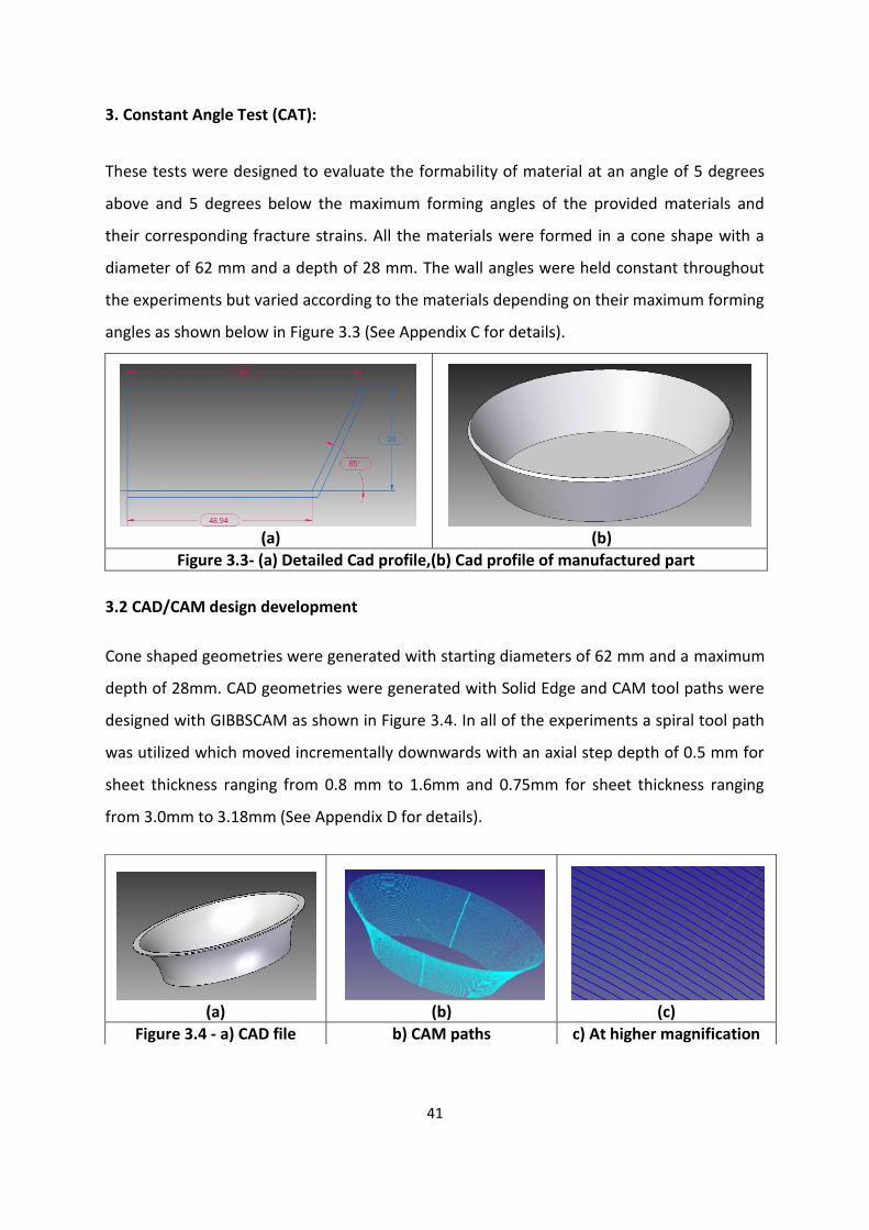
Figure 4.15- Force measurement (GAT) – Fx , Fy .......................................................................... 60
Figure 4.16- Force measurement (GAT) – Fz ................................................................................ 61

9
Figure 4.17- Tensile Strength Vs Fx, Fy ........................................................................................ 62
Figure 4.18- Multiple angle test AA6061 1.27 mm ....................................................................... 63
Figure 4.19- Maximum forming Angles ....................................................................................... 63
Figure 4.20- Fractured Surface .................................................................................................... 64
Figure 4.21- Maximum Thickness Strain ...................................................................................... 65
Figure 4.22- Thickness Strain Vs Tensile Strength ........................................................................ 66
Figure 4.23- Thickness Strain Vs Proof Stress ............................................................................... 67
Figure 4.24- Thickness Strain Vs Total Elongation (At) ................................................................. 67
Figure 4.25- Thickness Strain Vs Max. Elongation (Ag) ................................................................. 68
Figure 4.26- Force measurement (MAT) Fx, Fz ............................................................................. 69
Figure 4.27- Force measurement (MAT) – Fz ............................................................................... 70
Figure 4.28- Constant angle test AA6061 1.27 mm ...................................................................... 71
Figure 4.29- Constant forming Angles ......................................................................................... 71
Figure 4.30- Force measurement (CAT) Fx , Fy ............................................................................. 72
Figure 4.31- Force measurement (CAT) Fz ................................................................................... 73
Figure 4.32- Sheets etched with 2mm square grid Pattern ........................................................... 74
Figure 4.33- (a) Basic principle of electrochemical etching method, (b) Example of Stencil ........... 75
Figure 4.34- Strain Measurement Method .................................................................................. 75
Figure 4.35 – AA 2024-1.27 (CAT) 0° ............................................................................................ 76
Figure 4.36- AA 2024-1.27 (CAT) 90° ........................................................................................... 76
Figure 4.37 - Comparison Manual vs ASAME AA 2024-1.27 (CAT) 90° .......................................... 77
Figure 4.38- AA 2024-1.02 (CAT) 0° ............................................................................................. 78
Figure 4.39 - AA 2024-1.02 (CAT) 90° ........................................................................................... 78
Figure 4.40 - Comparison Manual vs ASAME AA 2024-1.02 (CAT) 90° .......................................... 79

10
List of symbols
Abbreviations (Acronyms)
KTH Kungliga Tekniska Hogskola
AA Aluminum Alloy
SPIF Single Point Incremental Forming
SMF Sheet Metal Forming
ISF Incremental Sheet Forming
ISMF Incremental Sheet Metal Forming
CNC Computer Numerical Control
CAM Computer Aided Manufacturing
CAD Computer Aided Drawing
GAT Geometric Accuracy Test
MAT Multiple Angle Test
CAT Constant Angle Test
RPM Revolution per Minute
FLC Forming Limit Curve
FFLs Fracture Forming Limit
FLA Fracture Line of Attack
FFLD Fracture Forming Limit Diagram
HTP Horizontal Top Planar
NGSVE Negative General Semi-Vertical Edge
PBSVE Positive Bottom Semi-Vertical Edge
PGSVR Positive General Semi-Vertical Ruled
HBP Horizontal Bottom Planar
NC Numerical Control
HRC Hardness Rockwell Scale
HB Hardness Brinell Scale
HV Hardness Vickers Scale
MOS2 Molybdenum disulfide
TDN Total Digestible Nutrients
Mpa Mega Pascal
ASAME Advances in measuring Surface Strain

11
Greek Symbols
Ø Forming Angle
Ø max Maximum Forming Angle
µ Coefficient of friction
α Drawing Angle (Sine Law)
σ Stress
σѲ Circumferential Stress
σØ Meridional Stress
є Strain
єt Thickness Strain
єѲ Circumferential Strain
єØ Meridional Strain
є1Biaxial Bi axial Strain
Є1Plane strain
Planar Strain
Latin Symbols
Δz Axial depth
Tf Final Thickness
To Original Thickness
n Strain Hardening Coefficients
K.n Strength and Strain Hardening Coefficients
r tool/t Tool radius to thickness Ratio
Rm Tensile Strength
Rp0.2 Proof Stress
Ag Maximum Elongation
At Total Elongation
G Shear Modulus
E Modulus of Elasticity
N Newton (Force)
Nm Newton Meter (Torque)
ln Natural Logarithmic

12
Chapter 1 Introduction
1.1 Background
During the past few years there has been increasing demand for the need of development
of manufacturing technologies that are both agile and be able to handle with the market
requirements, that is it should be also adaptable for new product development so that
introduction of new products in the markets could be easily achieved. Single point
incremental forming (SPIF) is a new innovative and feasible solution for the rapid
prototyping and the manufacturing of small batch sheet parts. The process is carried out at
room temperature (cold forming) and requires a CNC machining centre, a spherical headed
tool and a simple support to fix the sheet being formed. The flexibility of the process is
mainly related to the fact that SPIF does not require a dedicated die to operate as compared
to other forming processes. As a result, the lead-time and cost of tooling along with the die
cost can be avoided. This technique allows a relatively fast and cheap production of small
series of sheet metal parts [1]. The process starts from a flat sheet metal blank, clamped on
a sufficiently stiff rig and mounted on the table of a CNC machine. It can be used for forming
of symmetric and non-symmetric parts in a wide range of thicknesses from 100 microns up
to several mm [2].
(a)Metal Seat (b) Cone shape (c) Circular and Pyramid Shape
Figure 1.1 - A sample of manufactured parts
Figure 1.2 - Components formed using Macro incremental forming
Figure 1.2 -

13
In Single Point Incremental Forming (SPIF) specific terminologies are used which are
indicated in the following figure:
The incremental step-down size (Axial depth, Δz) is the amount of material deformed for
each passage of the forming tool (similar to cut depth in machining). The step size effects
both the machining time and the surface quality of the part produced and its value is set in
CAM software. Feed rate is the speed at which forming tool moves around the mill bed
(similar to cut rate in machining) and it directly effects the machining time for forming. It is
measured in mm/minute. The spindle speed is the rotation speed at which the tool rotates.
The spindle rotation speed varies the heat generated due to friction at the contact point
between the material and the forming tool and its values are also set in the CNC milling
machine along with the CAM software. The angle between the horizontal, under formed
sheet metal and the deformed sheet metal is defined as the forming angle (Ø). This is the
line of the deformed blank sheet metal as shown in Figure 1.3. The forming angle can be
used as a measure of material formability. The maximum angle (Ø max) is the greatest angle
formed in a shape without any failures. [1]
Figure 1.3 - SPIF terminology

14
1.2 Objectives
The objective of this work is to perform experiments to formulate a manufacturing process
for manufacturing of small aerospace components especially for SAAB Aerospace. In this
Study 3 different grade of Aluminium alloys were used namely AA 2024, AA 6061 and AA
7475 series alloys with plate thickness ranging from 0.8 mm to 3.18 mm.
The Main focus of this study was to organize a set of experiments to determine the forming
limits and the fracture points and the maximum forming angles for the above mentioned
materials in relation with four common SPIF forming parameters: step size, angle, spindle
speed, and feed rate and also to measure and analyze strain paths along the forming limits
and to determine the fracture strain for the above mentioned materials. The results
obtained should be able to predict and categorize the extent of the necking and thickness
reduction occurring before fracture along with the wall angle at which fracture initiated.
The second objective of this study is to determine the shape accuracy of the manufactured
parts in terms of depth achieved, thickness reduction and wall angles achieved in relation to
the CAD file. Tests were conducted on all the three grades of aluminium with different
thicknesses while keeping the experimental parameters constant which included spindle
speeds, step depth, feed rates and the tool radii in order to study the amount of deviation
that different materials show while comparing with the cad file.
Finally force evaluations were done in relation to the forming angles and different materials
used during the project.

15
1.3 Organization of Report
This thesis is organized in 5 different chapters including this introduction and a conclusion
summarizing the major contributions and outcomes of the research work along with the
suggested future work regarding this dissertation.
Chapter 2 concentrates on the literature review which includes review of the conventional
incremental forming processes used currently in the industrial practice along with this an
overview of the incremental forming processes, proceeds with the presentation of SPIF and
the identification of practical applications and the parameters that effect formability in
Single point incremental forming.
Lastly a discussion about the theoretical background of the SPIF process and concentrating
on fracture limits and forming limits diagrams in relation to the SPIF process along with the
geometric inaccuracy related to the profiles manufactured through SPIF and some of the
correction techniques for these in accuracies.
Chapter 3 gives a comprehensive description of the experimental techniques utilized for
material characterization and formability limits determination, an overview of the SPIF
experimental set-up and finally a short description of the CAD/CAM design development.
Chapter 4 presents the results and discussion related to 3 types of experiments performed
namely GAT, MAT and CAT and their analysis in terms of Geometric accuracy, fracture
strains, forces involved and true strains measurements. Along with this some comparisons
are also made in terms of geometric accuracy of the manufactured part with the CAD
profiles.
Finally, overall conclusions and future work are given in chapter 5. It is hoped that the
present work contributes towards a better understanding of the failure limits, forming limits
and geometry accuracy of SPIF manufacturing process.

16
1.4 References
1. M. Ham & J. Jeswiet, Single Point Incremental Forming and the Forming Criteria for
AA3003, Mechanical & Materials Engineering, Queen’s University, Kingston, ON,
Canada.
2. F. Vollertsen, H. Schulze Niehoff, H. Wielage, Z. Hu , Sheet Metal Micro Forming,
Bremer Institut für angewandte Strahltechnik - BIAS GmbH, ICIT & MPT 2007.

17
Chapter 2 Literature Review
2.1 Sheet Metal Forming Processes
Following are some of the most sheet metal forming processes commonly used forming
processes used in the modern day industry.
2.1.1 Hammering
Hammering is one of the oldest forming technologies, initially it was done manually but with
the time now it is also being performed with CNC. Modern Hammering processes takes
advantage of the robotic technology and it uses a robotic arm that controls the movement
of the tool and punches the sheet, which is clamped in a support frame, in circular
trajectories descending step by step in each round as shown in the figure 2.1[1].
Figure 2.1-Incremental Hammering process. (a) Incremental Hammering scheme (b) Industrial robot.
2.1.2 Spinning
Spinning can be divided in two different types:
• Conventional spinning • Shear spinning
Figure 2.2 - a) Conventional Spinning of a cone using multiple pass b) Shear Forming of a cone using a single pass.

18
In Conventional Spinning parts are gradually formed over a mandrel using a rounded tool or
roller. The equipment in case of spinning is quite similar to a lathe where the metal sheet is
clamped on the centre in a mandrel and then this whole setup is resolved. The tool applies a
localized pressure to deform the blank by axial and radial motions over the surface of the
part. The tool can be manual or mechanically actuated , the tool production cost is low in
this case as it is mostly suitable for producing small series parts involving low number of
sequence of steps for part manufacture.
Shear Spinning is quite similar to Conventional Spinning and the difference is the action
which is stretching instead of bending. This fact has a major influence on the variation of
thickness along the wall which follows the commonly known sine law (Tf =To Sin α) [2].
2.1.3 Stamping
Stamping processes are usually done through dedicated tooling usually called hard tools.
These processes are usually associated with high volume production of parts and are either
performed in single die station or multiple die station [3].The equipments of stamping can
be categorized to two types: mechanical presses and hydraulic presses. Mechanical presses
have a mechanical flywheel which stores the energy and then transfer it to punch to form
the part. They range in size from 20 tons up to 6000 tons. Strokes range from 5 to 500 mm
(0.2 to 20 in) and speeds from 20 to 1500 strokes per minute. Mechanical presses are well
suited for high-speed blanking, shallow drawing and for making precision parts where as
Hydraulic presses use hydraulics to deliver a controlled force. Tonnage can vary from 20
tons to 10,000 tons. Strokes can vary from 10 mm to 800 mm (0.4 to 32 in).Hydraulic
presses are suitable for deep-drawing,
compound die action as in blanking
with forming or coining. One of the
disadvantages of this process is the
high tooling cost as in order to increase
the tool or punch life it has to be
constantly sharpened along with the
cost related to the die which increases
the overall tooling cost [3].
Figure 2.3 Tool design for Hot Stamping Process

19
2.2 Single Point Incremental Forming
2.2.1 General SPIF Introductions
The emergence of a new sheet metal forming process known as Single Point Incremental
Forming (SPIF) has shown great promise in its diversity of use. Relative to other
conventional forming processes, SPIF offers more flexibility in forming capabilities and low
operating costs. It does not require any dedicated dies and it is ideal for rapid prototyping
and low production operations. Forming with this method involves the use of a multi-axis
CNC milling machine with a hemispherical tip tool. Unlike its close descendants, shear
forming and spinning, SPIF is able to form both axis symmetric and asymmetric shapes
because of computer assisted forming. Several advantages are easily realized with this
method. Its die less nature and simple forming rig along with the use of generic
hemispherical forming tools makes this process very versatile. Conversely, this is a low
volume production method because productivity and cycling time are affected by the size of
both the forming tool and the part being formed as well as the type of surface finish that is
desired.
A basic setup of a forming rig is shown in Figure 2.4 with all the components listed. This rig is
mounted to the worktable of the CNC milling machine and it becomes the platform for
forming. The clamping and top plates restrict flange material flow into the forming region
that is defined by tool path generated from the CAM software and due to this clamping
restriction tool applies much localized stresses to deform the sheet.
Figure 2.4- SPIF forming rig [4].

20
2.2.2 Important Forming Parameters
In SPIF the following are some of the important process parameters: Tool Path, sheet
material, forming angle, tool size, step size, forming speeds (rotation and feed rate),
lubrication, and shape. Each parameter is explained below as they pertain to general
forming and their respective influences on different observed effects.
Forming Tool path:
In order to form the part with SPIF first we have to generate a cad model and these cad
models are utilized for devising the tool paths using commercial CAM software’s. The CAD
package Solid Edge is used to create solid models of parts that are then imported into the
GibbCAM where the tool path is generated according to the profile of the CAD models. This
package is usually used for material removal in milling and is perfect for SPIF because its
built-in path generation algorithm can be used to guide the forming tool. Tool contours are
created and connected using a step or a spiral transition method. Figure 2.5 shows a
truncated cone that was formed
using step transition apart from
this continuous spiral tool paths
also used in order to achieve
smaller surface roughness and also
to avoid tool entry and exit marks.
Sheet Material:
Formability differs between materials and a statistical study by Fratini et al. tried to
establish the influence of common material properties on formability [6]. From their study,
they found that the strain hardening coefficient (n) as well as the interaction between the
strength and strain hardening coefficients (K.n), had the highest influence on formability.
This study showed that strain hardening coefficient, which differs greatly between
materials, had a marked influence on formability. Generally, higher hardening coefficient
will have higher formability.
Figure 2.5- Cone tool path contours [5].
21
Forming Angle:
The angle that the side walls of a part make with the horizontal xy-plane is known as
forming angle. The extent of this angle depends mainly on material properties and the sheet
thickness. Nonetheless, SPIF parts are controlled by the maximum forming angle (Ø max) to
which a material can be drawn before catastrophic failure in a single forming pass. Martins
et al. attempted to predict the maximum forming angle using material properties and
forming parameters as in Equation 2.1 [7].
Ø = /2−eεt Eq. 2.1
Where t is the fracture thickness at the limit of formability, the thickness strain is εt. In this
form, this equation can be readily evaluated using the through-thickness fracture limit strain
ε3 as determined from a plane strain or equi-biaxial stretch test. The equation represents
the onset of fracture because it combines the ideas of both the fracture forming limit in
principle strain space and the maximum forming angle at the onset of fracture [7].
Tool Size:
Tool size greatly affects both the formability and the surface finish of the manufactured part
through this process. Experiments have shown that smaller radius tools have higher
formability than larger ones. Larger tools have a bigger contact zone and tend to support
the sheet better during forming. Furthermore, in case of larger tool diameters there is an
increase in the amount of forming forces due to the increase in contact area between the
tool and the metal plate. In case of small diameter tools there is a highly concentrated zone
of deformation which results in high strains resulting in better formability. The decreased
forces observed with small tools means that lower stresses could be attained and as a result
there is smaller probability of the sheet to fail in low stress conditions. Higher formability
seen with small radius tools is thought be a consequence of the concentration of force and
strain as the surface area of contact is decreased at the tool tip. At this point, frictional
heating is very localized and high in magnitude. Both the high heating and strains are
thought to allow material to flow easily thus increasing formability [8].

22
Step Size:
The influence of step size on the formability along with how much it influences the SPIF
process is still a debatable parameter. Some researchers hold that step size does not
influence formability but rather it only affects surface roughness. While others believe that
it does influences formability and by increasing the step size there is a decrease in the
formability. In a study by Ham et al., it was shown that step size has an insignificant
influence on formability [9].It has been also noted that the step size not only affects the
outer and inner surface roughnesses but also has an effect on the duration of forming. Small
step sizes require more time to form parts since increasingly more z-plane motions are
necessary. The roughness influence however tends to be coupled with the immediate
forming angle of the particular part that is formed and also with the size of the tool.
Forming Speeds:
The influence of forming speed, both rotational spindle speed (RPM) and feed rate are
important regarding the SPIF process. The relative motion between the tool and sheet is
directly proportional to the heat that is generated by friction. Although it is generally
believed that formability increases with speed because of heating effects, there are several
tradeoffs and negative effects that may arise as a result. These include higher surface
roughness, increased tool wear rates, and lubricant film breakdown. Surface roughness
becomes coarser with increased speeds and surface defects such as sheet waviness become
more profound [10]. Forming at very high rotational speeds increases the likelihood of
developing tool chatter marks on the sheet [11].
Lubrication and Shape:
Lubrication in SPIF research has been limited. Discussions reach only as far as their friction
reduction tendencies and as a means to reduce tool wear and improve surface quality as it
is a relatively slow process related to machining or milling so tool wear is not one of the
major concerns but in case of warm forming lubrication plays a key role in terms of surface
roughness’s.

23
The geometric shapes that can be formed have a large effect on the forming forces and time
depending on complexity. According to the sine law, vertical walls are not possible with this
process because it would result in a zero final sheet thickness. Several techniques have been
used to improve this limitation including localized heating using laser and multi pass forming
[12, 13].The multi pass method involves forming a part with more than one forming pass.
Parts are formed from shallow to increasing angles at each pass until the desired shape is
achieved. Forming in multiple steps allows strains within the part to be applied gradually
rather than in a single increment. Experimentally, higher accuracies and formability are seen
with this method with better thickness distribution.
2.2.3 Multistage Forming
When forming through SPIF for a given material and thickness maximum forming angle can
be easily calculated with the help of cone forming test in which the angle is continuously
increased along with the depth and during that keeping all the other parameters constant
such as step size, feed rate and tool diameter. The tool paths used are conventional and
when a sufficiently portion of a work piece has a wall angle that exceeds the maximum
angle it results in the part failure.
The maximum wall angle limits the process and it is easy to see that it’s impossible to make
parts with right angle walls (i.e. at a drawing angle of 90 degree), because the wall thickness
in this conditions would be zero according to the sine law (Equation 2.2).
Tf=To Sinα Eq. 2.2
In this Tf is the final thickness of the manufactured part and To is the initial thickness and α is
the wall angle. It has been experimentally verified that the process follows this law with a
tendency to over form slightly.
To increase the maximum wall angle, the initial thickness of the sheet can be increased but
obviously this strategy has limitations on the maximum machine load and overall part
thickness specifications. The diameters of the tool and the selected step down also have an
influence on the maximum forming angle [14].
In order to achieve higher forming angles near to 90 degrees several authors have already
adopted multistage strategies. Consecutive tool paths, corresponding to virtual parts with

24
increasing wall angles, are being executed in a multi-step procedure. Typically a large offset
from the backing plate is favoured for the first passes since this allows for more bending,
avoiding extreme strains near the top of the part and after that the sheet is deformed in
successive turns to achieve higher angle in multiple passes. This strategy enables to reduce
the sheet thinning effect which leads to fracture and also to redistribute the material from
the bottom of the sheet which in case of SPIF remains untouched as a result higher forming
angles could be achieved with homogeneous sheet thickness [14].
Recently Skjoedt et al. [15] proposed a solution to obtain cones with vertical walls, for SPIF
without support through a forming strategy shown in the Figure 2.8.
Figure 2.6 -Thickness in function of radial dimension
Figure 2.7-Geometry and thickness in function of radius
Figure 2.8 - Five stage forming
.

25
2.2.4 Applications of Incremental Sheet Forming Process
Incremental Forming processes offer the possibility to implement a powerful alternative if
few products (small lot) have to be produced. And this possibility becomes a need in those
applications in which it is clear that the product has to be unique. The ISFP applications can
be separated in two different main areas:
Rapid prototyping for automotive industry, for example: reflexive surfaces for headlights see
Figure 2.9; a heat/vibration shield, see Figure 2.10; and silencer housing for trucks, see
Figure 2.11; etc.
Figure 2.9 - Reflexive surface for headlights [16]. Figure 2.10 - Automotive heat/vibration shield [17].
Figure 2.11 - Silencer housing for trucks [15].
Figure 2.12 - 1/8 scale model of front section of (Shinkansen) bullet train [18].
The medical field represents one of these cases which require high customisation, in order
to guarantee the best allowable performance of the product. Here is an example of
manufacturing of an ankle support, which is made starting from what we can roughly name
the “patient geometry”.

26
In other words, a reverse engineering
approach has been implemented in order to
manufacture the support directly starting
from the patient’s ankle shape, for ensuring
the best correspondence between the
obtained support and the patient body. Some
other possible fields of application for ISMF
are home appliances, aerospace and marine
industry.
2.3 Theoretical Background
In SPIF the mode of deformation has come under heavy discussion and different authors
have different opinions with some authors have the opinion that deformation occurs
through shearing [20] whereas other think it’s due to stretching [21].
Regarding the forming limits of SPIF there are three different views:
1. Formability in SPIF is limited by necking.
2. The Forming Limit Curve in SPIF is significantly higher than the conventional Forming
Limit curves (FLC) by an approximation of 2.7 times higher than conventional
processes e.g. (Stamping, deep drawing) [22].
3. This increase in the formability is due to large amount of through thickness shear or
due to serrated strain path arising from cyclic plastic deformation [23].
The alternative, and non-traditional, view of formability in SPIF recently proposed by Silva et
al. [24], and supported by Cao et al. [25], considers that:
1. Formability is limited by fracture without experimental evidence of previous necking.
2. The suppression of necking is the key mechanism for ensuring the high levels of
formability in SPIF.
3. FLC gives local necking strains so in case of SPIF it should be replaced by the Fracture
Forming Limits (FFLs). This approach is referred as the ‘fracture line of attack’ (FLA).
As conclusion, plane stretching is the principal mode of deformation in SPIF, and it is the
start point for the theoretical framework that will be presented in the following sections.
Figure 2.13 - 3D sketch of tool trajectory [19].
Figure 2.15 - Medical applications of ISMF. a) Cranial plate [24]. b) Dental plate[25].

27
2.3.1 Forming Limit Curves in Single Point Incremental Forming
Limits of a forming process are important to understand, as they give valuable insight in
failure prediction. In sheet metal forming (SMF),forming limits are determined through the
development of forming limit curves (FLC).FLC are plots of major and minor principle strains
which show a defined state and failure zone as FLC is usually measured after necking with
the measurement made just outside the necking zone as shown in the figure 2.14.
Traditional FLCs are used to predict failure in SMF, but lack the ability to estimate failure for
parts made with the SPIF process as a result fracture limit are used to predict failure which
are measured outside the fracture zone in SPIF.
Formability in SPIF can be defined in terms of the maximum draw angle and it is measured
in terms of a tangent line from the unformed sheet surface to the deformed surface.
Knowing Ø max can be the first step in determining whether the SPIF process is a good
forming application for a given material and sheet thickness. The forming limit curve in
incremental forming is quite different from the corresponding one in conventional forming
as shown in figure 2.14. Much higher strains may be achieved in incremental forming than in
traditional processes. Such circumstance can be justified taking into account the peculiarity
of the process mechanics. Plastic deformation induced by the small size punch is strongly
localized and confined to the close vicinity of the contact area, and then it incrementally
progresses as the tool moves along the assigned path. As a consequence higher strains can
be attained in the material before that fracture
occurs. Furthermore the forming limit curve for
incremental forming processes typically has the
shape of a straight line with a negative slope in the
first quadrant of the Forming Limit Diagram [26].
The FLD for SPIF is determined in two steps the first
one is single point incremental forming of the work
piece and the second one is grid measuring with
optical strain measuring system. Two different
deformations states are observed.
Figure 2.14 - AA 1050-0 Forming Limit Diagram

28
On flat surfaces the material flow mainly in the tool direction and plane strain is
originated on sheet metal.
On curved surfaces the sheet metal in deformed longitudinally and biaxial
deformation is developed in the sheet metal.
2.3.2 Crack propagation in rotational symmetric SPIF parts
In case of SPIF there are two modes of crack propagation [22].
• The circumferential “straight” crack propagation path • The circumferential “zigzag” crack propagation path The circumferential straight crack propagation path (Figure 2.15 c) is similar to that is found
in conventional deep drawing or stamping operations (Figure 2.15 d) and this type of crack
propagation is triggered due by stretching mechanism due to σØ. The zigzag crack
propagation path (Figure 2.15 b) is also triggered by σØ but its morphology that is zigzag
around the circumferential direction is probably due to friction caused by rotation of the
forming tool. The tip of the crack in (Figure 2.15 a) “a” will be under a much lower level of
meridional stresses than at the onset point “o”. Consequently, the propagation of the crack
stops and the rotation of the tool will drag it to point “b” which is similar to the initial point
“o” restarting the crack propagation. This cyclic mechanism gives the typical “zigzag”
morphology to the crack.
Figure 2.15 - Crack propagation in SPIF. a) Scheme of typical propagation path in SPIF.
b) Circumferential zigzag crack propagation path. c) Circumferential straight crack propagation path.
d) Circumferential straight crack propagation path (part obtained by conventional deep-drawing).

29
2.3.3 Forming limits
On the basis of study of the crack morphology and the measurement of the thickness along
the cross section of parts manufactured through SPIF it is revealed that plastic deformation
by uniform thinning until fracture without experimental evidence of necking taking place
[23]. The non presence of necking can be explained by the inability of neck to grow because
in that case it would have to grow around the circumferential bend path and overcome the
tool which is difficult to occur so it creates a problem for the neck development and even if
all conditions could be met at the small plastic deformation zone in contact with the tool,
growth will be inhibited by the surrounding material. As consequence of this, the FLCs of
conventional sheet metal forming are inapplicable to describe SPIF failure. FFLs curves
showing the fracture strains placed above the FLCs should be used in SPIF. The FFLD in SPIF
(Figure 2.16) can be
characterized by ductile
damage mechanics based on
void growth models. The
slope of the fracture forming
line (FFLD) in the principal
strain space (є1, є2) (Figure
2.16) can be given by the
following equation.
є1
Biaxial - є1Plane strain 5 (r tool/t) + 2 Eq. 2.3
є2Biaxial - 0 3 (r tool/t) + 6
For typical experimental values of (r tool/t) in the range 2–10 the slope derived from Equation
2.3 will vary between -1.0 and -1.4. This supports the assumption that the fracture forming
limit in SPIF can be approximately expressed as є1 + є2= q, where єt = -q is the thickness
strain at the onset of fracture in plane strain conditions. This result is in close agreement
with the typical loci of failure strains in conventional sheet forming processes, where the
slope of the FFLD is often about -1 [24].
Figure 2.16 - Schematic representation of the forming limits of SPIF against those of stamping and deep drawing
= -

30
2.3.4 Geometric Accuracy of the Parts
It has been observed that during forming through SPIF there are some deviations related to
the geometry of the part produced, one of the most common source of deviation is over
formability at low wall angles and low formability on high wall angles as a result when wall
angles are lower in range of 30 to 60 degrees there is an increase in formability and it
generally tends to over form the part being produced apart from this at high forming angles
above 60 to 80 degrees due to high spring back the formability is low in the part produced
[27].
It has been shown that tool path plays an important role in the final outcome and the
geometric accuracy of the path generated so tool path along with the features and features
interaction can be used to improve the accuracy of features in the part produced by SPIF.
Generally compensations are done in the CAD files of the part according to the predicted
deviations of individual features however in order to improve the accuracy of the entire part
it is also necessary to take into account the behaviours of each individual feature and all
feasible interaction between features [28].
2.3.5 Correction Techniques
A graph topology approach has been presented [29] which integrates the effect of
behaviour of all features present in the part, in this case a conceptual graph is constructed
representing all the features present in the part and connecting them based on their
location in the part with conceptual relations which helps to predict the amount of
deviations due to feasible interaction in an uncompensated part. Depending on the analysis
a comprehensive strategy for accurate path manufacture is devised which along with CAD
file compensation also may include complementary tool path strategies.
The set conceptual relations are based on experimental knowledge how features interact
with each other covering specific requirements that features need to meet with respect to
the positioning and alignment regarding part functionality specification and once all the
features are recognized and connected through conceptual relations it form the complete
graph of the part. See figure 2.17 and 2.18.

31
Example of Conceptual Graph for a cone shaped geometry:
Figure 2.17 - Relations used for feature based graph topology definition [29]
Figure 2.18 - Conceptual C-graph for a cone (Feature abbreviations [29] - HTP: Horizontal Top Planar NGSVE: Negative General Semi-Vertical Edge PGSVR: Positive General Semi-
Vertical Ruled HBP: Horizontal Bottom Planar PBSVE: Positive Bottom Semi-Vertical Edge)
The above figures represent the utility of these graphs in terms of analysis of feature
behaviour and feature interactions. In the above cone the surface represented as Feature 3
is the major source of inaccuracy as it tends to under deform due to spring back in
moderate to high wall angle parts. The other sources of inaccuracy include near the backing
plate where horizontal top planar feature (Feature 1) and cone (Feature 3) form a negative
semi vertical edge (Feature 2) which creates a zone of over forming and in the same manner
Feature 5 is formed deep due to compression in the radial direction during the part
manufacture and creates so called Tent or Pillow effect.
Integrated Accuracy Improvement Strategy Generation Improvement in accuracy of complete parts can be achieved by following a three step
procedure: [29]
1. Identify part features and their interaction that results in accuracies.
2. Introduce compensation strategies for each individual feature and interaction based
on the knowhow for the specific feature or interaction.
3. Selecting out of the listed strategies a comprehensive set of complementary
strategies for the complete part.

32
2.3.6 Economic Analysis of SPIF
Due to high cost of die in sheet metal forming, conventional forming processes are suitable
only for high-volume production. However the pattern of demand for sheet metal product
has undergone a change, which necessitates small-batch sizes. Single point incremental
forming is a die-less forming process and can be employed for customizes sheet metal
products made in small quantity [1]. Though the cost of the die is less, the cost of machine
tool is high in this case. Cost models for two types of parts have also been proposed. A sheet
metal product is usually produced with dies and punches manufactured in accordance with
shape and dimension of the components. Production in low series and small batches
induces higher demands on the production system as a whole and short decision times are
important. Apart from adapting the organization to low volume, the right forming process
must be chosen. Regarding the forming process, the following guidelines can be used for
efficient low volume production: Reduced -lead-time for each product, and reduced
changeover time between products, Reduced time and cost for development and
manufacturing of tool, Flexible production units and production lines Lower time between
different products by using flexible tooling, e.g. incremental forming or fluid forming. [30]
Break Even Analysis
Break-even analysis is based on categorizing
production costs between those, which are
“variable” (costs that change when the
production output changes) and those that
are “fixed” (costs not directly related the
volume of production). Total variable and
fixed costs are compared with sales revenue
in order to determine the level of sales
volume, sales value or production at which
the business makes neither a profit nor loss.
Figure 2.19 - Schematic of breakeven point

33
In the diagram above, the line OA represent the variation of income at varying levels of
production activity i.e., output. OB represents the total fixed costs in the business. As output
increases, variable costs are incurred, meaning that Total Cost/Product = Fixed Cost +
Variable Cost/Product also increases. At low levels of output, total cost/product is greater
than income. At the point of intersection P, total cost is exactly equal to income, and hence
neither profit nor loss is made. Fixed cost consists of, for conventional forming, press
machine, dedicated dies etc. and for SPIF NC (Numerical Control) Machine. Variable costs
are sheet metal and direct labour and will be same for both the processes. However, the
level of skill required to operate the machine and wastage of sheets will be different in the
two cases.
Figure 2.20 - Conventional Vs SPIF
Production cycle of incremental forming is shorter than the conventional production. The
forming paths are generated directly from the 3D CAD and often no tooling is needed. If a
support tool is required, the same 3D CAD is used for making the support tool. The support
tool materials are inexpensive and easy to work, and a new support tool can be made fast
when needed. If corrections are needed, the CAD file is changed, the programme is
converted again and the next piece can be manufactured. Corrections to the model are easy
to make in any part of the process [30].

34
Cost Models
Comparison between ISF (Incremental Sheet Metal Forming) and Stamping is carried out for
the forming of various shapes with different degrees of geometrical complexities i.e. car
hood, oil tank cover, cup shape, pyramid with various radii. The Cost Model for ISF
(Incremental Sheet Metal Forming) and Stamping are constructed by using estimated costs
of dedicated die (fixed cost), machine (fixed cost), personnel cost (variable cost) etc.
Break Even Models for Different Products
Figure 2.21- Car hood Figure 2.22- Oil tank cover Figure 2.23- Pyramid
It is clear from these break-even points that whatever the geometry of part produced
incremental forming has much lower break even. It shows that the breakeven point have
slight dependence on the size of the part produced in the case of incremental forming. For
relatively large parts; there is an increase in the breakeven point as compared to smaller
part in ISF [30].
ISF Cost Rs/
Time min
Stamping Cost Rs/
Time min
Personal Cost 3000/hr Personal Cost 3000
Machine Cost 3000/hr Machine Cost 3000
CAM Development 30 min Die Setting up time 30 min
Part Forming 30 min Part Forming 5 sec
Die Cost 27500 Die Cost 600000
Table 1- Cost Comparison – ISF and Stamping

35
2.4 References
1. Schafer T., Schraft R.D., Incremental sheet metal forming by industrial robots using a
hammering tool, 10emes Assises Europeennes de Prototypage Rapide, Paris, France
(2004).
2. Hagan E. and Jeswiet J., A review of conventional and modern single point sheet
metal forming methods. Journal of Engineering Manufacture, 217 (2003) 213-225.
3. Nam Ho Kim, Kyung Kook Choi, Jiun Shyan Chen Die shape design optimization of
sheet metal stamping process using mesh free method International Journal for
Numerical Methods in Engineering, Volume 51, Issue 12, (2001), 1385-1405.
4. Joost R. Duflou, Joris Dhondt, Applying TRIZ for systematic manufacturing process
innovation: The single point incremental forming case, Procedia Engineering 9
(2011), pages 528-537.
5. Flores, P. Duchene, L. Bouffioux, C. Lelotte, T. Henrard, C. Pernin, N. Van Bael, A. He,
S. Duflou, J. Habraken, A.M. Model identification and FE simulations: Effect of
different yield loci and hardening laws in sheet forming. International Journal of
Plasticity, 23 (2007), 420-449.
6. Fratini, L., Ambrogio, G., Di Lorenzo, R., Filice, L. Micari, F. The influence of
mechanical properties of the sheet material on formability in single point
incremental forming. CIRP Annals. 53(2004), 207-210.
7. Martins, P.A.F. Bay, N. Skjoedt, M. Silva, M.B. Theory of single point incremental
forming. Journal of Strain Analysis. 43(2008), 15-35.
8. Engenharia Mecanica, Dissertation Master Thesis, University of Lisbon, September
(2009).

36
9. Ham M, Jeswiet J., Single point incremental forming and the forming criteria for
AA3003, CIRP Annals, 55(2006). 241-244.
10. Hagan, E., Jeswiet, J. Analysis of surface roughness for parts formed by computer
numerical controlled incremental forming. Proc. IMechE. J. Engineering
Manufacture. 218(2004), 1307-1312.
11. Jeswiet J, Micari F, Hirt G, Bramley A, Duflou J, Allwood, J., Asymmetric single point
incremental forming of sheet metal, CIRP Annals, 54(2005), 623-650.
12. Isekia, H. Naganawab, Vertical wall surface forming of rectangular shell using
multistage incremental forming with spherical and cylindrical rollers. Journal of
Materials Processing Technology. 130(2002), 675–679.
13. Duflou, J.R Callebaut, B. Verbert, J. De Baerdemaeker, H. Laser Assisted Incremental
Forming: Formability and Accuracy Improvement. CIRP Annals, 56(2007),273-276.
14. J.R. Duflou, J. Verbert, B. Belkassem , J. Gub, H. Sol, C. Henrard, A.M. Habraken,
Process window enhancement for single point incremental forming through multi-
step tool paths CIRP Annals - Manufacturing Technology 57 (2008) 253-256.
15. Skjoedt M., Bay N., Endelt B. and Ingarrao G., Multi-stage strategies for single point
incremental forming of a cup, 11th ESAFORM conference on metal forming (2008).
16. Jeswiet J., Hagan E., Rapid proto-typing of a headlight with sheet metal, Proceedings
of Shelmet (2001) 165-170.
17. Jeswiet J., Recent results for SPIF. Seminar on Incremental Forming, Cambridge
University (2004) CdRom.

37
18. Jackson, K.P. and Allwood, J.M. (2008) The mechanics of incremental sheet forming,
Journal of Materials Processing Technology, 209(3) 1158-1174.
19. G. Ambrogio, L. De Napoli, L. Filice, F. Gagliardi, M. Muzzupappa, Application of
Incremental Forming process for high customised medical product manufacturing
Journal of Materials Processing Technology 162–163 (2005) 156–162.
20. Rodrigues J.M.C., Martins P.A.F., Tecnologia da Deformacao Plastica: Aplicacoes
Industriais, Escolar Editora (2005).
21. Silva MB, Skjoedt M, Atkins AG, Bay N, Martins PAF (2008) Single Point Incremental
Forming & Formability/Failure Diagrams. Journal of Strain Analysis for Engineering
Design 43(1):15–36.
22. Silva MB, Skjoedt M, Atkins AG, Bay N, Martins PAF (2008) Revisiting the
fundamentals of single point incremental forming by means of membrane analysis.
International Journal of Machine Tools & Manufacture 48 (2008): 73-83
23. Allwood J.M., Shouler D.R., Tekkaya A.E., The increased forming limits of incremental
sheet forming processes, Key Engineering Materials 344 (2007) 621-628.
24. Silva M.B, Single Point Incremental Forming, PhD Thesis, Instituto Superior Tecnico
Portugal (2008).
25. P.A.F. Martins, N. Bay, M. Skjoedt, M.B. Silva Theory of single point incremental
forming. CIRP Annals – Manufacturing Technology 57 (2008) 247-252.
26. M. Ham and J. Jeswiet, Mechanical and Materials Engineering, Queen’s University,
Kingston, ON, Canada, Forming Limit Curves in Single Point Incremental Forming,
CIRP Annals Vol. 56/1/2007, pages 277-280.

38
27. J. Verbert, J. Duflou, B. Lauwers, Feature based approach for increasing the accuracy
of the SPIF process, Key Engineering Materials 344 (2007) 527-534.
28. A.K. Behera, H. Vanhove, B. Lauwers, J.R. Duflou, Accuracy Improvement in Single
Point Incremental Forming Through Systematic Study of Feature Interactions, Key
Engineering Materials 473 (2011) 881-888.
29. Amar Kumar Beheraa, Bert Lauwersb, Joost R. Duflouc An Integrated Approach to
Accurate Part Manufacture in Single Point Incremental Forming using Feature Based
Graph Topology Key Engineering Materials Vols. 504-506 (2012) 869-876.
30. Syed Asad Raza Gardezi Economic Analysis of low volume sheet metal products
manufactured by single point incremental forming process. A M.Sc Manufacturing
thesis, UET, Lahore 2008.

39
Chapter 3 Experimental work
This section starts with giving the overview of the experimental techniques that were
utilized for material characterization and follows by introducing the technique utilized for
determining the material forming limits, the description of experimental SPIF setup utilized
the plan of experiments and the CAD/CAM design development performed. The
experiments were conducted in order to evaluate the following parameters:
Geometric Accuracy Test (GAT)
Multiple Angle Test (MAT)
Constant angle test (CAT)
The experiments were designed in order to evaluate the shape accuracy of the part
manufactured through SPIF along with fracture strains and the maximum forming angles for
the provided materials as mentioned in the chapter 2.
3.1 Plan of experiments
There were 3 sets of experiments as shown below and all the experiments were double
tested to check the reliability and the reproducibility of the experiments. The spindle speeds
of 100 rpm and feed rate of 1500 mm/min were held constant throughout the experiments.
For all the experiments 12 mm diameter tool was used for thicker material (3.0mm-
3.18mm) and 8 mm diameter tool was used for thinner material (0.8mm-1.6mm). The axial
depth for thicker sheets was kept constant at 0.75 mm and for thinner sheets was 0.5 mm
throughout the experiment.
Material (mm) Tool (mm) Axial Depth
(mm)
GAT MAT CAT
(Above)
CAT
(Above)
AA 2024 (1.02) 8 0.5 2 pieces 2 pieces 2 pieces 2 pieces
AA 2024 (1.27) 8 0.5 2 pieces 2 pieces 2 pieces 2 pieces
AA 2024 (3.18) 12 0.75 2 pieces 2 pieces 2 pieces 2 pieces
AA 6061 (0.8) 8 0.5 2 pieces 2 pieces 2 pieces 2 pieces
AA 6061 (1.27) 8 0.5 2 pieces 2 pieces 2 pieces 2 pieces
AA 7475 (0.8) 8 0.5 2 pieces 2 pieces 2 pieces 2 pieces
AA 7475 (1.6) 8 0.5 2 pieces 2 pieces 2 pieces 2 pieces
AA 7475 (3.0) 12 0.75 2 pieces 2 pieces 2 pieces 2 pieces
Table 2 – Plan of Experiments

40
1. Geometric Accuracy Tests (GAT):
These tests were designed to evaluate the geometric accuracy of the part manufactured
through single point incremental forming. All the materials were formed in a cone shape
with a diameter of 62 mm and a depth of 26 mm. The wall angles ranged from 40 to 60
degrees. The variation of angle form 40 to 60 degrees along the conical profile was in 5
steps and each step had a depth of 5 mm except the initial step which was of 6 mm as
shown below in Figure 3.1 (See Appendix C for details).
(a) (b)
Figure 3.1- (a) Detailed Cad profile,(b) Cad profile of manufactured part
2. Multiple Angle Test (MAT):
These tests were designed to evaluate the maximum forming angles of the provided
materials and their corresponding fracture strains. All the materials were formed in a cone
shape with a diameter of 62 mm and a depth of 27 mm. The wall angles ranged from 45 to
85 degrees. The variation of angle form 45 to 85 degrees along the conical profile was in 9
steps and each step had a depth of 3 mm as shown below in Figure 3.2(See Appendix C for
details).
(a) (b)
Figure 3.2- (a) Detailed Cad profile,(b) Cad profile of manufactured part
41
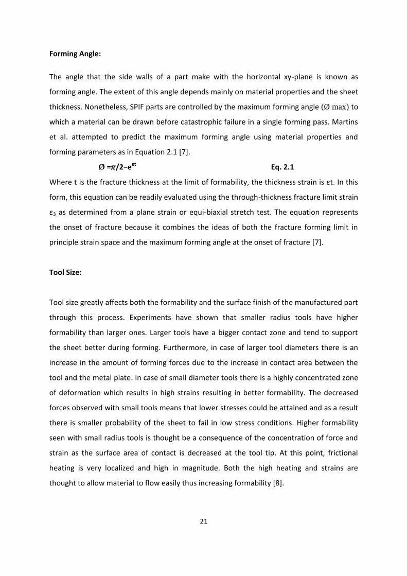
3. Constant Angle Test (CAT):
These tests were designed to evaluate the formability of material at an angle of 5 degrees
above and 5 degrees below the maximum forming angles of the provided materials and
their corresponding fracture strains. All the materials were formed in a cone shape with a
diameter of 62 mm and a depth of 28 mm. The wall angles were held constant throughout
the experiments but varied according to the materials depending on their maximum forming
angles as shown below in Figure 3.3 (See Appendix C for details).
(a) (b)
Figure 3.3- (a) Detailed Cad profile,(b) Cad profile of manufactured part
3.2 CAD/CAM design development
Cone shaped geometries were generated with starting diameters of 62 mm and a maximum
depth of 28mm. CAD geometries were generated with Solid Edge and CAM tool paths were
designed with GIBBSCAM as shown in Figure 3.4. In all of the experiments a spiral tool path
was utilized which moved incrementally downwards with an axial step depth of 0.5 mm for
sheet thickness ranging from 0.8 mm to 1.6mm and 0.75mm for sheet thickness ranging
from 3.0mm to 3.18mm (See Appendix D for details).
(a) (b) (c)
Figure 3.4 - a) CAD file b) CAM paths c) At higher magnification

42
3.3 Experimental Setup
Description of the Experimental setup is described in the following subsections which
include description of the CNC machine, tools used, lubrication used and the clamping
system utilized during the tests.
3.3.1 CNC Machine
All the tests were performed at Department of Production engineering at KTH Royal
Institute of Technology on 3 axis Mazak Mazatrol Machining centre as shown in the figure.
Figure 3.5 – 3 Axis Mazak Mazatrol Machining Centre
CNC operating System Mazatrol CAMM-2
Number of Axis 3
Machining Capacity (mm) 762/381/508
Max. Tool Diameter (mm) 100
Table 3- Machine Technical Specification

43
3.3.2 Forming tools
The tools were made from Cold work Uddeholm RIGOR steel hardened to 65 HRC with
hemispherical tips. Two different diameters were used regarding tools (8 mm and 12 mm).
The basic idea behind using tools of two different diameters were to check the formability
of the material with regards to tool radius and sheet thickness ratio and also to observe the
effect on tool diameter as we change from small diameter that is 8 mm to larger diameter
that is 12 mm on surface roughness, fracture point and necking and the shape accuracy of
the manufactured parts.
In our experimentation 12 mm tools were used for thick sheets that have thickness up to
3.18 mm and 8 mm tools were used for thinner sheets that have thickness up to 1.6 mm
(See Appendix A for details).
Figure 3.6 – Tool Holder Figure 3.7 – 8, 12 mm Diameter tool
Tool material Uddelholm Rigor
Material Composition 1%C and 5%Cr
Delivery State hardness 215HB
Hardness Condition HRC 65 and HRC 57
Tempering Condition 200°and 300°
Table 4- Tool Technical and Material Specification

44
3.3.3 SPIF clamping system
The CNC machine to perform SPIF made use of a dedicated clamping system as shown in the
Figure 3.8 (See Appendix B for details).
The complete clamping system displayed in Figure 3.8 (c) is composed by the static frame (a)
fixed on the machine working table, the blank holder (b) to hold the sheet over the backing
plate. The whole apparatus is clamped to the bottom corners of the working table of the
CNC by eight M8 screws. The working area of the forming process was 250 mm by 350 mm.
In this study unlike proposed in chapter 2, there was no utilization of the backing plate
which was considered an important factor in terms of geometric accuracy of the part
manufactured, so one of the objectives of the current study to see the effect on the
geometric accuracy of the part manufactured without backing plate and how compensation
techniques can be applied without using of the backing plate to gain the desired geometric
accuracy. The non usage of the backing plate also is a step forward to make this process
more economical and rapid manufacturing process as exclusion of the backing plate not
only reduces the cost of the experimentation but also reduces the setup times.
3.3.4 Lubrication Conditions
The application of lubricant in ISMF is important to obtain a smooth surface and to reduce
the wear of the tool. Bramley [1] observed that the type of lubricant is not a principal factor.
Later, Carrino et al [2] concluded that friction differences in SPIF are only obvious in
comparison between the process with and without lubrication.
Figure 3.8 - (a) Die b) Blank holder c) Including sheet

45
In this project 2 types of lubricants were used
Molybdenum disulfide (MOS2)
Castrol Illoform TDN 81
Both of the lubricants were used in form of a thin film over the sheet being formed in form
of a lubricant pool where the forming tool was constantly dipped while the forming
operation took place. The spindle speed and the feed rate were held constant while testing
the effect of the two lubricants at 100 rpm and 1500 mm/min.
The surface wear, see Figure 3.9, 3.10, 3.11 appeared during forming of the annealed plates
made from material AA 2024, AA 6061 and AA 7475 performed with Molybdenum disulfide
MOS2 along with the chipping effect which was observed in thicker sheets (3 mm- 3.18 mm).
Figure 3.9 – AA 2024 3.18 mm sheet Figure 3.10 – AA 6061 1.27 mm sheet
Figure 3.11 – AA 7475 3.0 mm sheet

46
Therefore to avoid this and to reduce the impact of friction between the forming tool and
the sheet Castrol Illoform TDN 81 was tested under the same process conditions on the
material AA 2024, AA 6061 and AA 7475.
The parts lubricated by Castrol IloformTDN 81 forming fluid, shown in Figure 3.12, 3.13 and
3.14 reached substantially better surface quality roughness, when compared with the MOS2
as shown above. Also the tool wear was reduced mainly because Castrol IloformTDN 81
provides better lubrication due to its excellent boundary lubrication properties [6].
The boundary (film) lubrication is based on the bonding arranged between the forming tool
and the blank sheet by fine close-fitting lubrication and during the process as the
temperature rises due to friction between the forming tool and the sheet formed the
reactive constituents of the lubricant react with the contact surface forming a highly
resistant tenacious layer, or film on the moving solid surfaces (boundary film) which is
capable of supporting the load, the major wear and avoiding the breakdown.
Figure 3.12 – AA 2024 1.27 mm sheet Figure 3.13 – AA 6061 1.27 mm sheet
Figure 3.14 – Al 7475 1.6 mm sheet

47
3.3.5 Material used
Generally three different grades of Aluminium alloys were used namely AA 2024, AA 6061
and AA 7475 and for each grade of materials there were various thicknesses available
ranging from 0.8 mm to 3.18 mm. Following are the list of the materials used during the
experimentation.
Material Thickness (mm) Sheet Area (cm)
AA 2024 1.02,1.27,3.18 250 x 350
AA 6061 0.8,1.27 250 x 350
AA 7475 0.8,1.6,3.00 250 x 350
Table 5- Material Specification
The sheets were provided by SAAB Aerospace Sweden in annealed condition with 500 cm in
length and 500 cm in breadth which were later cut to 250 x 350 mm sheets as shown in the
figure 3.15.
(a) (b) (c)
Figure 3.15 – (a) AA 2024 sheet, (b) AA 6061 sheet, (c) AA 7475 sheet

48
Material characterization of AA 2024 (Cu-Mg-Aluminium)
Property Symbol Units Value
Tensile Strength 1.02 mm Rm MPa 181
1.27 mm 184
3.18 mm 187
Proof Stress 1.02 mm Rp0.2 MPa 70
1.27 mm 95
3.18 mm 91
Maximum Elongation 1.02 mm % Ag 15.3
1.27 mm 13.6
3.18 mm 15.1
Total Elongation 1.02 mm % At 19.6
1.27 mm 19.0
3.18 mm 16.9
Shear Modulus G MPa 27 000
Modulus of Elasticity E MPa 73 000
Table 6- Material characterization AA 2024
Material characterization of AA 6061 (Mg-Si-Cu-Cr-Aluminium)
Property Symbol Units Value
Tensile Strength 0.8 mm Rm MPa
120
1.27 mm 117
Proof Stress 0.8 mm Rp0.2 MPa 53
1.27 mm 62
Maximum Elongation 0.8 mm % Ag 20.5
1.27 mm 22.2
Total Elongation 0.8 mm % At 27.7
1.27 mm 27.8
Shear Modulus G MPa 26 000
Modulus of Elasticity E MPa 68 000
Table 7- Material characterization AA 6061

49
Material characterization of AA 7475 (Zn-Mg-Cu-Cr-Aluminium)
Property Symbol Units Value
Tensile Strength
0.8 mm Rm
MPa 205
1.6 mm 185
3.0 mm 190
Proof Stress 0.8 mm Rp0.2 MPa 96
1.6 mm 91
3.0 mm 94
Maximum Elongation 0.8 mm % Ag 12.2
1.6 mm 9.5
3.0 mm 13.2
Total Elongation 0.8 mm % At 15.2
1.6 mm 11.0
3.0 mm 13.8
Modulus of Elasticity E MPa 69 000
Shear Modulus G MPa 26 200
Table 8- Material characterization AA 7475
3.4 References
1. Bramley A.N., Incremental Sheet Forming Process for small batch and prototype
parts, Verlag Meisenbach (2001) ISBN 3-87525-149-0.
2. Carrino L., Di Meo N., Sorrentino L., Strano M., The influence of friction in negative
dieless incremental forming, 9th ESAFORM International Conference on Materials
Forming, Glasgow, UK (2006) 203-206.

50
Chapter 4 Results and Discussion
4.1 Results
As discussed earlier 3 series of test were conducted namely GAT, MAT and CAT. The results
from the following three series of experiments are mentioned in the following chapter. This
chapter presents an analysis of the geometric accuracy of the parts manufactured through
single point incremental forming with relation to the original CAD/CAM profile. Along with
this analysis of fracture limits, maximum forming angles and fracture strains in correlation
with the forces and tensile strength of the material mentioned in chapter 3.
4.2 Measuring method:
1. Depth Measurement
Depth measurements were done with digital venire Calliper with a least (0.01mm) as shown
in figure 4.1.
2. Diameter Measurement
Marking were made at every 5 mm (± 0.5 mm) depth and the diameter were measure with
the help of venire calliper as shown in the figure 4.2.
(a) (b) (c) (d)
Figure 4.2- (a),(b) Outer diameter measure, (c),(d) Inner diameter measure
Figure 4.1 –Depth measurement with venire calliper

51
3. Angle Measurement
The angle measurement of the wall angles of the part manufactured was done through on
screen angle measurement mode. The setup consisted of Cannon Power shot SX40 Hs used
at the objective lens setting of 35X (24 mm wide), and the manufactured part (figure 4.3 a).
The camera and the sheet metal part were placed at a distance of 90 cm with the part
elevated above the surface by 30 cm (figure 4.3 b) in order to match the bottom plane of
the manufactured part with the centre of the camera lens. The slope of the manufactured
part was measured with the help online angle measurement ruler as shown in figure 4.3 c.
4. Thickness measurement
Measurements were made with Micrometer Screw Gauge with a least count of (0.001mm).
(a) (b)
Figure 4.4 - a) Sheet markings, b) Measurement with screw gage
(a)
(b)
(c)
Figure 4.3 - a) Angle measurement setup, b) Sheet position, c) On screen angle measure
30 mm 90 cm

52
4.3 Geometric Accuracy Test (GAT)
In this section results related to GAT are presented. For geometric accuracy test all the
materials were formed at an angle ranging from 40 to 60 degrees to a depth of 26 mm and
following factors were evaluated against the CAD and CAM models.
4.3.1Thickness measurement
Following is the graphs of thicknesses from top to bottom of the part manufactured as a
function of depth for the aluminium alloys tested.
Figure 4.5 – Thickness graph along the depth profile of the part manufactured
As it is visible from the graph that all the alloys follows a set pattern in terms of thickness
reduction and the thickness is reduced from top to bottom as the wall angle increases. The
highest thickness reduction of approximately 80 percent was achieved in case of AA 6061
alloy and the lowest in case of AA 7475 alloys which was about 50 percent of thickness
reduction as compared to the original sheet thickness. It can also be seen that thickness
reduction is different as the thickness of the metal sheet changes as in case of thicker sheets
the reduction is less as compared to the thinner sheets.
0
0,5
1
1,5
2
2,5
3
3,5
0 5 10 15 20 24 25 Bottom
Thic
knes
s (m
m)
Thickness Vs Depth
AA 2024 1.02
AA 2024 1.27
AA 2024 3.18
AA 6061 0.8
AA 6061 1.27
AA 7474 0.8
AA 7475 1.6
AA 7475 3.0

53
Thickness strains were calculated from the data presented in the figure 4.5 through the
equation 4.1 for each material.
Thickness Strain =ln (Tf/To) Equation 4.1
Where Tf is the thickness at the point where the strain is being measured as shown in figure
4.4 and To is the original sheet thickness.
Figure 4.6 – Maximum Thickness Strain
Figure 4.7 –Thickness Strain Vs Depth Profile of the CUP
-0,9
-0,85
-0,8
-0,75
-0,7
-0,65
-0,6
-0,55
AA2024 1.02
AA 2024 1.27
AA 2024 3.18
AA 6061 0.8
AA 6061 1.27
AA 7475 0.8
AA7475 1.6
AA 7475 3.0
Thic
kne
ss S
trai
n =
ln (
Tf/T
o)
Material
Thickness Strain GAT
Thickness Strain 1
Thickness Strain 2
-1,4
-1,2
-1
-0,8
-0,6
-0,4
-0,2
0
0 5 10 15 20 24 25 bottom
Thic
knes
s St
rain
(ln
(Tf
/To
))
Depth (mm)
Thickness Strain Vs Depth
AA 2024 1.02
AA 2024 1.27
AA 2024 3.18
AA 6061 0.8
AA6061 1.27
AA 7475 0.8
AA 7475 1.6
AA 7475 3.0
Tf=To Sinα

54
As it can be observed in the figure 4.6 and 4.7 it gives us a clear indication of relation
between the percentage thickness reduction and the amount of thickness stain generated in
the sheets of different materials during the test performed. In case of thicker sheets that is
AA 2024-3.18mm and AA 7475-3.0 mm, the usage of higher diameter tool results in low
amount of local plastic forming which results in lower strain values for these sheets as
compared to the thinner sheet materials which are formed with small diameter tool of 8
mm. As small radius concentrates the strain at the area of deformation in the sheet under
the forming tool and a large radius tends to distribute the strains over a more extended
area. It can also be concluded from the figure that high amount of strains are generated in
the lowest thickness sheets due to the fact of large amount of stretching in the negative z
axis direction during forming operation.
4.3.2 Depth measurement
Figure 4.8 –Attained and Cad Depth Comparison
The following figure 4.8 shows a comparison between the original CAD part depths along
with the depth achieved during the experiments for different aluminium alloys. These
depths are measured form the clamped section of the sheet till the base of the part
manufactured. As it is visible from the graph that a pattern is developed showing higher
depth achievement in case of increased initial sheet thickness. The highest depth of 26.3
24,6
24,8
25
25,2
25,4
25,6
25,8
26
26,2
26,4
Al 2024 1.02mm
Al 2024 1.27 mm
Al 2024 3.18 mm
Al 6061 0.8 mm
Al 6061 1.27 mm
Al 7475 0.8 mm
Al 7475 1.6 mm
Al 7475 3.0 mm
De
pth
(m
m)
Materials
Cad Depth
Attained Depth

55
mm is achieved by the thickest aluminium alloy sheet which is AA 2024-3.18 mm due to the
fact that as the thickness of the sheet increases higher forces are required to form the sheet
which results in higher initial sheet bending at the edges of the clamped sheet along with
the effect of higher amount of spring back in case of thinner sheets as compared to the
thicker sheets.
4.3.3 Diameter vs. Depth measurement
Figure 4.9 –Attained and Cad diameter Comparison
Figure 4.10 –Attained and Cad diameter Comparison
70 75 80 85 90 95
100 105 110 115 120 125 130
25 20 15 10 5 0
Dia
me
ter
(mm
)
Depth (mm)
Diameter vs Depth AA 2024
CAD Diameter
AA 2024 1,02
AA 2024 1,27
AA 2024 3,18
70 75 80 85 90 95
100 105 110 115 120 125 130
25 20 15 10 5 0
Dia
me
ter
(mm
)
Depth (mm)
Diameter vs Depth AA 6061
CAD Diameter
AA 6061 0,8
AA 6061 1,27

56
Figure 4.11 –Attained and Cad diameter Comparison
Here comparisons were made between the original CAD diameters and actual diameters of
the part produced through SPIF. As seen from figure 4.9-4.11 that thinner sheet metal
aluminium alloys whose thickness range from 0.8 mm to 1.6 mm show a quite good fit with
the CAD model where as the thicker alloys with thickness ranging from 3.0 mm to 3.18 mm
show around 10 percent deviation in case of the bottom measure of the diameter due to
the usage to larger diameter tool.
70
75
80
85
90
95
100
105
110
115
120
125
130
25 20 15 10 5 0
Dia
me
ter
(mm
)
Depth (mm)
Diameter vs Depth AA 7475
CAD Diameter
AA 7474 0,8
AA 7475 1,6
AA 7475 3,0

57
4.3.4 Depth vs. forming angle measurement
Figure 4.12 –Attained and Cad Wall Angle Comparison
As shown in the figure 4.12 a comparison is made between the CAD wall angles and the
obtained original angles from the part manufactured and as it is seen that all the materials
show a quite good fit to the original Cad angles after the depth of 10 mm where as initially
at a depth from 0 to 5 mm the formability is low as compared to the cad profile which is due
to the influence of the tool radius vs. thickness ratio as increasing the R/t ratio reduces the
spring back in most cases [1], as a result we observe high level of spring back in AA 2024-
3.18 (R/t=1.88) as compared to AA 2024 -1.27 (R/t=3.14) which results in the initial
deviation of the wall angle formed. Whereas this effect is diminished as the forming
operation continues, this is due to the fact of constant reduction in thickness during the
forming operation which results in increased R/t ratio and consequently reducing the spring
back.
30
35
40
45
50
55
60
65
25 20 15 10 5
Wal
l An
gle
Depth (mm)
Wall Angle Vs Depth
CAD Wall Angle
AA 2024 1,02
AA 2024 1,27
AA 2024 3,18
AA 6061 0,8
AA 6061 1,27
AA 7474 0,8
AA 7475 1,6
AA 7475 3,0

58
Test case of AA 6061 - 1.27 mm
For further investigation of geometric accuracy one of the manufactured parts of AA 6061-
1.27 mm was sent to EXOVA AB for thickness, harness and surface roughness measures.
Point Thickness
(mm)
Reduction
percentage %
1 0.67 47 %
2 0.68 46 %
3 0.74 42 %
4 0.92 28 %
5 1.17 8 %
6 1.26 0.8 %
Surface 1.27 0 %
Figure 4.13 - Thickness measured by Infrared Table 9 – AA6061 - 1.27 mm, Percentage Thickness reduction
Hardness measure
Point 1-2 Hardness (HV) Point 4-5 Hardness (HV)
Max. Hardness 59 Max. Hardness 54
Min. Hardness 55 Min. Hardness 46
Medium Hardness 57 Medium Hardness 51
Standard Deviation 2 Standard Deviation 4
Point 2-3 Point 5-6
Max. Hardness 57 Max. Hardness 45
Min. Hardness 55 Min. Hardness 43
Medium Hardness 56 Medium Hardness 44
Standard Deviation 1 Standard Deviation 1
Point 3-4
Table 10 – AA6061 - 1.27 mm, Hardness measure(HV, 0.01)
Max. Hardness 55
Min. Hardness 54
Medium Hardness 54
Standard Deviation 0

59
Surface roughness measure
Surface roughness values were gathered from both the outer and inner side of the part
manufactures as shown in the figure 4.14. The outer surface roughness points are indicated
by 1, 2, 3 and the inner surface roughness points are indicated by 4, 5, 6 and on each point 3
measurements were taken represented by B (Base) , M(Medium), T(Top) surface roughness.
(a) (b)
Figure 4.14- a) Outer surface roughness measure, b) Inner surface roughness measure
Points B M T Points B M T
1 0.801 µ 0.814 µ 1.072 µ 4 0.503 µ 0.585 µ 0.511 µ
2 0.718 µ 0.625 µ 0.972 µ 5 0.710 µ 0.658 µ 0.567 µ
3 0.751 µ 0.836 µ 1.140 µ 6 0.418 µ 0.701 µ 0.565 µ
Table 11 –AA 6061- 1.27mm, Outer and inner surface roughness measure
As indicated by the surface roughness values in Table- 11 it is concluded that better surface
roughness are obtained through SPIF on the inner side where the forming tool rotates to
form the path as compared to the outer untouched region of the part manufactured. One of
the reasons of high surface roughness values on the outer side of the manufactured part is
high amount of strain induced during the forming process.
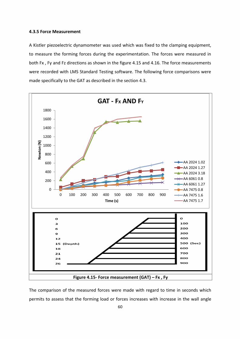
60
4.3.5 Force Measurement
A Kistler piezoelectric dynamometer was used which was fixed to the clamping equipment,
to measure the forming forces during the experimentation. The forces were measured in
both Fx , Fy and Fz directions as shown in the figure 4.15 and 4.16. The force measurements
were recorded with LMS Standard Testing software. The following force comparisons were
made specifically to the GAT as described in the section 4.3.
Figure 4.15- Force measurement (GAT) – Fx , Fy
The comparison of the measured forces were made with regard to time in seconds which
permits to assess that the forming load or forces increases with increase in the wall angle
0
200
400
600
800
1000
1200
1400
1600
1800
0 100 200 300 400 500 600 700 800 900
Ne
wto
n (
N)
Time (s)
GAT - FX AND FY
AA 2024 1.02
AA 2024 1.27
AA 2024 3.18
AA 6061 0.8
AA 6061 1.27
AA 7475 0.8
AA 7475 1.6
AA 7475 1.7

61
that is from 40 to 60 degrees in this case and the forming depth and the tool size as it can be
seen in figure 4.15 and 4.16 showing higher amount of forces generated when the tool
diameter was changed form 8 mm to 12 mm.
As shown in the figure 4.13 the forces measures for Fx and Fy direction are same for each
material due to the cup shaped geometry of the part which results in circular motion of the
tool equally in both X and Y axis while the part is manufactured along with negative Z axis
movement of tool with an increment of 0.5 mm for thin sheets and 0.75 mm for thicker
sheets with every contour of circular motion of tool represented by Fz force as shown in
figure 4.14. In case of Fx and Fy force the highest amount of force was obtained for AA 7475
3.0 mm which is about 1600 N where as the lowest was obtained for AA 6061 0.8 mm which
perfectly coincides with the tensile strength of the respective materials as shown in the
figure 4.17.
Figure 4.16- Force measurement (GAT) – Fz
Whereas when we look to the forces measures in the Fz direction the magnitude of the
forces are quite low as compared to what we observe in Fx and Fy direction which is due to
the fact of incremental spiral movement of the tool in the negative Fz direction.
0
10
20
30
40
50
60
0 100 200 300 400 500 600 700 800 900
Ne
wto
n (
N)
Time (s)
GAT - Fz
AA 2024 1.02
AA 2024 1.27
AA 2024 3.18
AA 6061 0.8
AA 6061 1.27
AA 7475 0.8
AA 7475 1.6
AA 7475 1.7

62
Here we see a correlation between the product of tensile strengths and thicknesses of
different materials with their corresponding Fx and Fy forces ad we can conclude that as the
tensile strength is increased higher amount of forces are generated during the forming
forces and the increase of the forces in mainly dependent on the material properties along
with the thickness as we see a major shift in the amount of forces required to form the part
when changing form thinner to thicker sheet which in this case are AA 2024 3.18 mm and
AA 7475 3.0 mm.
Figure 4.17- Tensile Strength Vs Fx, Fy
AA 2024 1.02
AA 2024 1.27
AA 2024 3.18
AA 6061 0.8
AA 6061 1.27 AA 7475 0.8
AA 7475 1.6
AA 7475 3.0
90
190
290
390
490
590
690
0 200 400 600 800 1000 1200 1400 1600 1800
Ten
sile
Str
en
gth
x T
hic
kne
ss
Force (Fx, Fy) (N)
Tensile Strength VS Fx, Fy

63
4.4 Multiple Angled Tests (MAT)
In this sections results are presented regarding
MAT in order to evaluate the maximum forming
angles and the their corresponding fracture strains
and then some correlations were made with the
tensile strength of the individual materials and
their fracture strains and lastly forces were
evaluated for each material. The part
manufactured was a cone shape with angles
ranging from 45 to 85 degrees and a depth of 27
mm as shown in figure 4.18.
4.4.1 Maximum forming Angle
Figure 4.19- Maximum forming Angles
As seen from the figure the maximum forming angle was achieved in case of AA 6061 of 75
degrees and the minimum for AA 7475 of 60 degrees before fracture, as shown in the figure
4.19 that regardless of the thickness of the sheet all the materials that belong to same
category of alloys showed the same maximum forming angle. Two series of
experimentations were carried out for MAT and both of them gave the same results as
presented in the figure 4.19.
Figure 4.18- Multiple angle test AA6061 1.27 mm
50
55
60
65
70
75
AA2024 1.02
AA2024 1.27
AA2024 3.18
AA6061 0.8
AA6061 1.27
AA7475 0.8
AA7475 1.6
AA7475 3.0
An
gle
MAT 1 MAT 2

64
4.4.2 Fracture surfaces
Two modes of crack propagation were observed as shown in the Figure 4.20. The
circumferential straight crack propagation path (Figure 4.20d,f) is similar to that is found in
conventional deep drawing or stamping operations and this type of crack propagation is
triggered due by stretching mechanism due to circumferential stress (σØ).
The zigzag crack propagation path (Figure 4.20a,c,e) is also triggered by (σØ) but its
morphology that is zigzag around the circumferential direction is probably due to friction
caused by rotation of the forming tool as discussed in chapter 1.
AA 2024 AA 6061 AA 7475
(a, AA 2024-1.02mm) (d, AA 6061-0.8 mm) (f, AA 7475-0.8 mm)
(b, 2024-1.27mm) (e, AA 6061-1.27mm) (g, AA 7475-1.6 mm)
(c, AA 2024-3.18mm)
Figure 4.20- Fractured Surface
(h, AA 7475-3.0 mm)
o a
b
c
d
e
f
σØ
σØ

65
4.4.3 Strains measurements
Thickness Strain
The thickness strains were measured as mentioned in section 4.3.1. Figure 4.21 presents the
maximum thickness strains noted for MAT. The values were noted just before the fracture
and as seen from the figure 4.21 highest amount of strains were noted for AA 6061 alloys
reaching up to -1.89 which is approximately 3 times higher values as compared to values
obtained during conventional forming operations and the lowest values were obtained for
AA 7475 alloys.
One of the other observations that could be made is the considerable amount of difference
in thickness strains when comparing maximum thickness strains of thick (3.0 mm- 3.18 mm)
and thin sheets (0.8 mm- 1.6 mm).
Figure 4.21- Maximum Thickness Strain
-2
-1,6
-1,2
-0,8
-0,4 Al 2024 1.02
Al 2024 1.27
Al 2024 3.18
Al 6061 0.8
Al 6061 1.27
Al 7475 0.8
Al 7475 1.6
Al 7475 3.0
Thic
kne
ss S
trai
n =
ln (
Tf/T
o)
Material
Thickness Strain 1
Thickness Strain 2

66
When corresponding these thickness strains values were plotted against the tensile strength
of different materials tested as shown in the figure 4.22 it can be observed that higher the
tensile strength of the material will be able to generate lower strains before fracture while
lower the tensile strength results in higher generation of thickness strains as it can be
observed in figure 4.22 for the case of AA 6061. For thicker sheets where large diameter
tool was used to form the part the correlation of the tensile strength and the thickness
strain is same as observed for the thinner sheets and shown in the figure 4.20 that AA 7475
3.0 mm having higher tensile strength than AA 2024 3.18 mm, which results in higher
thickness strains in AA 2024 3.18 mm as compared to AA 7475 3.0 mm before fracture. So it
can be concluded that keeping the all the process conditions constant higher thickness
strains before fracture are generated in the material that posse’s lower tensile strength.
Figure 4.22- Thickness Strain Vs Tensile Strength
AA 2024 1.02 AA 2024 1.27
AA 2024 3.18
AA 6061 0.8 AA 6061 1.27
AA 7475 0.8
AA 7475 1.6
AA 7475 3.0
-2
-1,8
-1,6
-1,4
-1,2
-1
-0,8
-0,6
-0,4
-0,2
0
100 120 140 160 180 200 220
Thic
knes
s St
rain
= ln
(Tf
/To
)
Tensile Stength (MPA)
Thickness Strain Vs Tensile Stength (Rm)
Thickness Strain 1
Thickness Strain 2

67
Figure 4.23- Thickness Strain Vs Proof Stress
A same sort of pattern is observed when comparing thickness strains with the proof stress
of their respective materials and as shown in the 4.23 the lower the proof stress higher the
amount of thickness strains are generated before fracture.
Figure 4.24- Thickness Strain Vs Total Elongation (At)
AA 2024 1.02 AA 2024 1.27
AA 2024 3.18
AA 6061 0.8 AA 6061 1.27
AA 7475 0.8 AA 7475 1.6
AA 7475 3.0
-2,1
-1,9
-1,7
-1,5
-1,3
-1,1
-0,9
-0,7
-0,5
-0,3
50 60 70 80 90 100
Thic
knes
s St
rain
= ln
(Tf
/To
)
Proof Stress (MPA)
Thickness Strain Vs Proof Stress (Rp0.2)
Thickness Strain 1
Thickness Strain 2
AA 2024 3.18
AA 6061 1.27
AA 7475 0.8 AA 7475 1.6
AA 2024 1.02
AA 2024 1.27
AA 6061 0.8
AA 7475 3.0
-2
-1,8
-1,6
-1,4
-1,2
-1
-0,8
-0,6
-0,4
-0,2
0
0 5 10 15 20 25 30
Thic
knes
s St
rain
= ln
(Tf
/To
)
Total Elongation (At) %
Thickness Strain Vs Total Elongation (At)
Thickness Strain 1
Thickness Strain 2

68
Figure 4.25- Thickness Strain Vs Max. Elongation (Ag)
From the data presented in the above figures (4.24, 4.25) we can make the following
observations:
The highest maximum elongation (Ag) and the highest total elongation (At) are shown by
the materials where highest thickness strains are obtained before fracture as show in the
above figures as in case of AA 6061 which shows both the highest maximum and total
elongation and also the highest thickness strains as compared to all the other aluminium
alloys before fracture where as the thicker materials that are AA 2024 3.18 mm and AA 7475
3.0 mm showing the lowest amount of maximum and total elongation along with the least
amount of thickness strains accumulated before fracture .
It can be concluded from the above figures that thickness strains is linearly related to the
maximum and total elongation. Higher the elongation higher will be the thickness strains
before fracture.
AA 2024 1.02
AA 2024 1.27
AA 2024 3.18
AA 6061 0.8
AA 7475 3.0
AA 6061 1.27
AA 7475 0.8 AA 7474 1.6
-2
-1,8
-1,6
-1,4
-1,2
-1
-0,8
-0,6
-0,4
-0,2
0
0 5 10 15 20 25
Thic
knes
s St
rain
= ln
(Tf
/To
)
Maximum Elongation (Ag) %
Thickness Strain Vs Max. Elongation (Ag)
Thickness Strain 1
Thickness Strain 2

69
4.4.4 Force measurements
The following force comparisons were made specifically to the MAT as described in the
section 4.4.
In case of Fx and Fy the highest amount of force was obtained for AA 7475 3.0 mm which is
about 1800 N where as the lowest was obtained for AA 6061 0.8 mm around 150 N which
perfectly coincides with the tensile strength of the respective materials as shown in the
section 3.3.5.
Figure 4.26- Force measurement (MAT) Fx, Fz
0
200
400
600
800
1000
1200
1400
1600
1800
2000
0 100 200 300 400 500 600 700 800
Ne
wto
n (
N)
Time (s)
MAT - Fx, Fy
AA 2024 1.02
AA 2024 1.27
AA 2024 3.18
AA 6061 0.8
AA 6061 1.27
AA 7475 0.8
AA 7475 1.6
AA 7475 1.7

70
Figure 4.27- Force measurement (MAT) – Fz
Whereas when we look to the forces measures in the Z axis direction we observe the same
kind of behaviour as observed in figure 4.16 that the magnitude of the forces are quite low
as compared to what we observe in Fx and Fy direction which is due to the fact of
incremental spiral movement of the tool in the negative Fz direction.
0
10
20
30
40
50
60
70
80
0 100 200 300 400 500 600 700 800 900
Ne
wto
n (
N)
Time (s)
MAT - Fz
AA 2024 1.02
AA 2024 1.27
AA 2024 3.18
AA 6061 0.8
AA 6061 1.27
AA 7475 0.8
AA 7475 1.6
AA 7475 1.7

71
4.5 Constant Angled Tests (CAT)
In this section tests were conducted out at constant
angle, 5 degrees below and 5 degrees above the
maximum forming angles of the given material, the
maximum forming angles were determined in
multiple angle test described in the section above.
The part manufactured was a cone shape with a
depth of 28 mm as shown in figure 4.28.
4.5.1 Constant forming Angle
Figure 4.29- Constant forming Angles
As seen from the figure the forming angle achieved in case of constant angle test were
according to the maximum forming angles predicted above as all the materials except
AA2024-3.18 mm were formed without any failure at 5 degrees below the maximum
forming angle and the part fractured immediately when tests were conducted at 5 degrees
above the maximum forming angle for all materials. Two series of experimentations were
carried out for CAT and both of them gave the same results as presented in the figure 4.29.
Figure 4.28- Constant angle test AA6061 1.27 mm
50
55
60
65
70
AA2024 1.02
AA2024 1.27
AA2024 3.18
AA6061 0.8
AA6061 1.27
AA7475 0.8
AA7475 1.6
AA7475 3.0
An
gle
CAT 1 CAT 2

72
4.5.2 Force measurements
The following force comparisons were made specifically to the CAT as described in the
section 4.5.
Figure 4.30- Force measurement (CAT) Fx , Fy
In case of X and Y axis force the highest amount of force was obtained for AA 7475 3.0 mm
which is about 1600 N where as the lowest was obtained for AA 6061 0.8 mm around 170 N
which perfectly coincides with the tensile strength of the respective materials as shown in
the section 3.3.5.
0
200
400
600
800
1000
1200
1400
1600
1800
0 100 200 300 400 500 600 700 800 900
Ne
wto
n (
N)
Time (s)
CAT - Fx , Fy
AA 2024 1.02
AA 2024 1.27
AA 2024 3.18
AA 6061 0.8
AA 6061 1.27
AA 7475 0.8
AA 7475 1.6
AA 7475 1.7

73
Figure 4.31- Force measurement (CAT) Fz
Whereas when we look to the forces measures in the Z axis direction we observe the same
kind of behaviour as observed in figure 4.31 that the magnitude of the forces are quite low
as compared to what we observe in Fx and Fy direction which is due to the fact of
incremental spiral movement of the tool in the negative Fz direction.
0
10
20
30
40
50
60
70
0 100 200 300 400 500 600 700 800 900 1000
Ne
wto
n (
N)
Time (s)
CAT - Fz
AA 2024 1.02
AA 2024 1.27
AA 2024 3.18
AA 6061 0.8
AA 6061 1.27
AA 7475 0.8
AA 7475 1.6
AA 7475 1.7

74
4.5.3 Strain Measurement
The principal methods used over here for strain and deformation measurement was the grid
marking method. Due to the simplicity of this method it is one of the commonly used strain
measurement methods for strain analysis in sheet metal forming. It consists of a very small
diameter circle or square grid pattern whereas grid marking is the process of printing line
patterns in the area of interest on the sheet metal blank. In our case the sheets were
electrochemically etched with a square pattern of a size of 2 mm at Swerea Kimab as shown
in the figure 4.32.
(a) (b)
Figure 4.32- Sheets etched with 2mm square grid Pattern
The basic principle of this method is shown in figure 4.33 [1]. The experimental equipment
required to generating the grid pattern on the blank consist of a low voltage power source,
stencil, felt pad, and etching solution. Initially the power source is attached to the electrode
and the sheet blank. A desired pattern stencil is then carefully placed on the surface of the
sheet which in our case was a square grid pattern of area 2 mm by 2 mm as shown in figure
4.33 (b). Now an electric voltage is applied for approximately 5 seconds and a roller type
electrode wheel with an attached power source is reciprocated on the felt pad and thus
current is passed from the electrode to the blank resulting in pressing out of the etching
solution through the contours of the stencil on the surface of the sheet by means of the
pressure generated by the roller wheel. After etching, the sheet metal is washed with a
neutralizing solution. Thus square grid pattern is generated as shown in figure 4.32.

75
Figure 4.33- (a) Basic principle of electrochemical etching method, (b) Example of Stencil
The measurements were made in ASAME (Automated Strain Analysis and Measurement
Environment) Version 4.12. ASAME Technology offers two main types of strain
measurement systems. One of these is a single point strain analysis system, and the other is
a multiple point strain and geometry analysis system [2]. In our case single point analysis
system was used. It uses a video camera and software which measures one grid element,
such as a circle or square at a time and computes major and minor strains at the relevant
grid. The samples were measured along two strips, one at 0 degree direction (horizontal
side) and one strip in the 90 degree direction (vertical side) as shown in the figure 4.34.
Figure 4.34- Strain Measurement Method

76
Strain analysis was conducted for the parts manufactured through CAT. The material tested
were AA 2024 1.02mm and AA 2024 1.27 mm as shown from the figure 4.35-4.40.
Figure 4.35 – AA 2024-1.27 (CAT) 0°
Figure 4.36- AA 2024-1.27 (CAT) 90°

77
As seen from the figure 4.35 and 4.36 the major strain values were obtained for AA 2024-
1.27 (CAT) at B0 and B 90 , where B0 represents the measurements taken at horizontal
plane at 0 degrees as shown in the figure 4.34 where as B 90 represents the measurements
taken at vertical plane at 90 degrees.
The deformed strip as shown in the figure 4.35 and 4.36 are divided into small square grid
pattern where the strains are measured according to ASAME (Automated Strain Analysis
and Measurement Environment) technology and each of the small boxes are represented by
colour pattern ranging from light blue to dark brown colour pattern. The light blue colour
represents the lowest strains region and the brown section represents the highest strain
region.
According to the data mentioned above in figure 4.35 and 4.36 the strain levels in both the
direction B0 and B90 are quiet similar due to the circular profile of the manufactured part
which enables a homogenous distribution of strain all over the circular wall where the
highest amount of strains are reached in the middle of the manufactured part represented
by the dark brown colour and the strain values reaching up to 0.91 in case of horizontal
direction and 0.93 in case of vertical direction. The lowest strain levels of 0.01 in the
horizontal direction and 0.04 in the vertical direction are observed at the beginning and the
ending region of the formed part.
Figure 4.37 - Comparison Manual vs ASAME AA 2024-1.27 (CAT) 90°
0
0,2
0,4
0,6
0,8
1
1,2
0 5 10 15 20 24 25 28
Thic
kne
ss S
trai
n
Depth (mm)
Comparison Manual vs ASAME
Thickness Strain Manual
Thickness Strain ASAME

78
A comparison of the strain levels were done between the strain levels calculate theoretically
as mentioned in section 4.3 and 4.4 and the strain levels measured through ASAME
technique and as seen from the figure that there is a quite good fit between the both
theoretical and experimental measurements.
Figure 4.38- AA 2024-1.02 (CAT) 0°
Figure 4.39 - AA 2024-1.02 (CAT) 90°
79
According to the data mentioned above in figure 4.38 and 4.39 the strain levels in both the
direction F0 and F90 were also quiet similar due to the above mentioned reason. The strain
values reached up to 0.91 in case of horizontal direction and 0.96 in case of vertical
direction. The lowest strain levels of 0.009 in the horizontal direction and 0.04 in the vertical
direction were observed at the beginning and the ending region of the formed part.
Figure 4.40 - Comparison Manual vs ASAME AA 2024-1.02 (CAT) 90°
A comparison of the strain levels were also done between the strain levels calculate
theoretically as mentioned in section 4.3 and 4.4 and the strain levels measured through
ASAME technique for AA 2024-1.02 (CAT) 90° and as seen from the figure similar results are
observed.
Form this it can be concluded that during the SPIF process homogeneous strains are
originated all over the walls and due to the nature of the process which is incremental,
localized forming higher strains level are achieved as compared to the conventional
processes such as stamping or deep drawing which enables of achievement of higher depths
without reaching the fracture strain.
0
0,2
0,4
0,6
0,8
1
1,2
0 5 10 15 20 24 25 28
Thic
kne
ss S
trai
n
Depth (mm)
Comparison Manual vs ASAME
Thickness Strain Manual
Thickness Strain ASAME

80
4.6 References
1. Siegert K. and Wagner S., 1994, Formability Characteristics of Aluminium Sheet,
Training in Aluminium Application Technologies (TALAT).
2. Fahrettin Ozturk, Murat Dilmec, Mevlut Turkoz, Grid Marking and Measurement
Methods for Sheet Metal Formability , 5th International Conference on Design and
Production of Machines and Dies, June 2009.

81
Chapter 5 Conclusion and Future Work
5.1 Conclusion
The research work developed in this MSc thesis project was aimed to analyze the formability
limits and mechanisms of aluminium metal sheets namely AA 2024, AA 6061 and AA 7475
during SPIF. For that 3 kind of tests were performed namely GAT, MAT and CAT for the
purpose of evaluation of geometric accuracy of the part manufactured along with the
determination of the maximum forming limit or maximum forming angles for the respective
materials tested. The experiments were performed changing the diameters of the tools and
the material conditions such as material thickness that were utilized for producing parts by
the SPIF process.
In this thesis work one of the major advancements were to perform the experimental
procedures without the aid of the backing plate unlike most of the work done regarding
single point incremental forming and it could be concluded that by using of proper thickness
to tool diameter ratio and choosing proper tool path, parts can be made with high
accuracies without the use of the backing plate as described in chapter 4. This is one of the
major advancements in terms of the modern industrial setups as it allows reducing the
setup costs along with the fixture cost.
In terms of formability of the materials, high level of formability were achieve as compared
to conventional forming processes and from the three aerospace graded Aluminium alloys
provided to us by SAAB it was concluded that highest formability level was achieved by AA
6061 alloy in terms of both geometric accuracy and in maximum wall angles followed by AA
2024 and the lowest for AA 7475 alloys.
High amount of strain levels were archived through SPIF process as due to local straining
high thickness reductions were observed as compared to conventional forming processes
exceeding by an amount of 50 percent. Form the strain measurements it can be concluded
that highest amount of strain level achieved before fracture were in case of thin sheets
(0.8mm- 1.6 mm) as compared to thick sheets (3.0mm- 3.18 mm) as due to localized

82
forming higher strains level are achieved as compared to the conventional processes such as
stamping or deep drawing which enables of achievement of higher depths without reaching
the fracture strain.
A correlation was found between the tensile strength of the material and the stains levels
observed and it was shown that material with higher tensile strength were able to generate
lower thickness strains before fracture while material with lower tensile strength results in
higher generation of thickness strains as mentioned in chapter 4. Similarly it can also be
concluded that thickness strains are linearly related to the maximum elongation (Ag) and
total elongation (At). Higher the elongation higher will be the thickness strains before
fracture.
The experiments performed in this thesis, allowed to observe the existence or absence of
necking in the parts made by SPIF and to conclude that necking exists only in the parts made
with bigger diameter tools, because the process is more similar to that of conventional
stamping.
Lastly some comparisons were made regarding the level of forces observed during the
forming process and a linear relationship was observed between the product of thickness
and tensile strength verses the level of forces observed to form the part. The level of forces
observed were ranged from 500 Newton to 2000 Newton’s which is quite low in accordance
to the modern industrial manufacturing operations such as stamping , cutting and milling.

83
5.2 Future work
Experimentation and analysis from these test revealed several areas that need further
study. They are listed below.
First of all to study multi stage forming regarding single point incremental forming and to
manufacture parts in multiple steps rather than one single step as one of the limitations
observed in this master dissertation was formability of vertical walls as in all the
experiments the tool paths were chosen such that deformation occurred on linear strain
paths so it would be interesting to go a step ahead and choose non linear strain path in
order to increase the formability limit as the main limitations of this process in formation of
perpendicular walls or in other case achieve 90 degrees wall angle as in that case
theoretically according to sin law the sheet thickness is reduced to zero but by adopting to
non linear strain paths higher wall angles could be achieved so multi-stage SPIF presents a
strategy for manufacturing parts, with vertical walls which would enable to form complex
shaped parts.
Secondly to study the surface and geometric accuracies. To manufacture part with multiple
planes and to study their geometric accuracies and comparisons with the CAD files and for
enhancing their accuracies regarding tool paths and different compensation techniques
regarding sheet material and the effect each plane has on the other plane in terms of
geometric accuracy.
At last devising a process strategy for integration of SPIF in the factory line, measuring the
process life cycle and to provide a replacement for the conventional forming processes. The
idea of Forming Mobile Factory and to develop the process of Single Point Incremental
forming such that it can act like portable small factories.
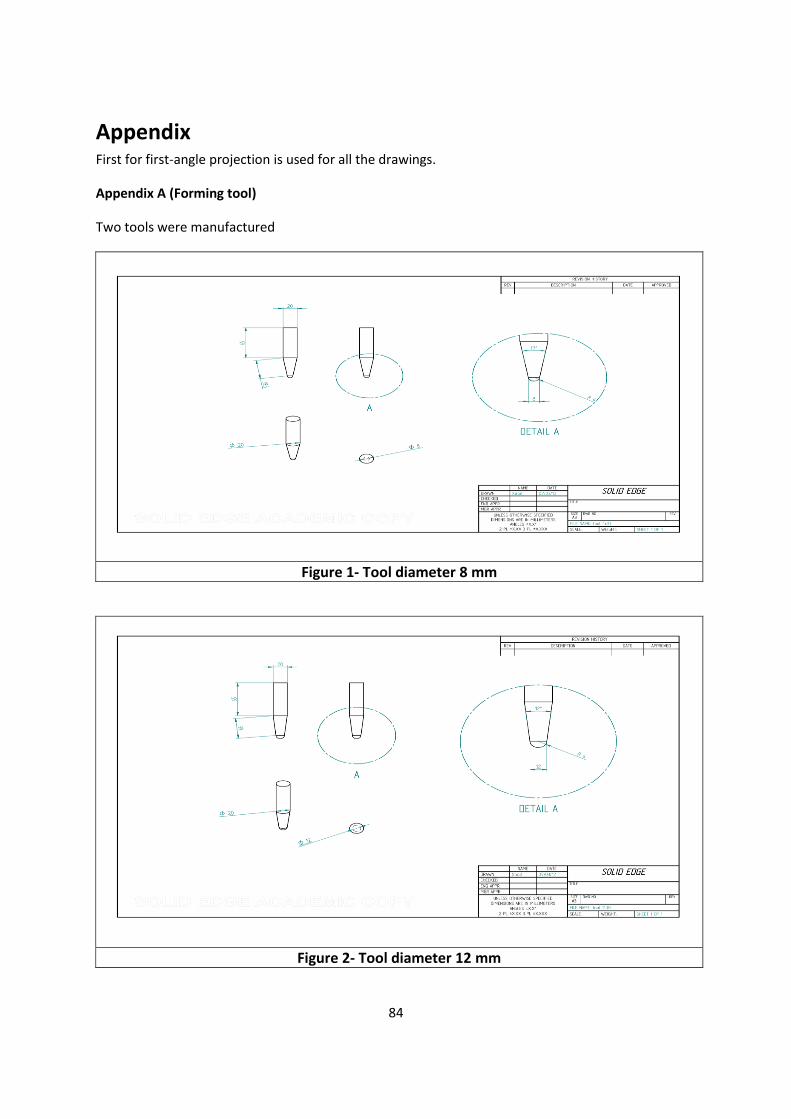
84
Appendix First for first-angle projection is used for all the drawings.
Appendix A (Forming tool)
Two tools were manufactured
Figure 1- Tool diameter 8 mm
Figure 2- Tool diameter 12 mm
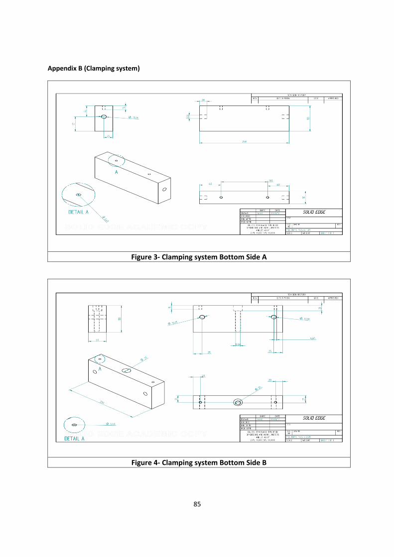
85
Appendix B (Clamping system)
Figure 3- Clamping system Bottom Side A
Figure 4- Clamping system Bottom Side B

86
Figure 5- Clamping system Top Side A
Figure 6- Clamping system Top Side B

87
Appendix C (CAD profiles)
1. Geometric Accuracy Tests (GAT):
(a) (b)
Figure 7- (a) Detailed Cad profile,(b) Cad profile of manufactured part
Figure 8- Cup for geometric Accuracy Test

88
2. Multiple Angle Test (MAT):
(a) (b)
Figure 9- (a) Detailed Cad profile,(b) Cad profile of manufactured part
Figure 10- Cup for Multiple Angle Test

89
3. Constant Angle Test (CAT):
(a) (b)
Figure 11- (a) Detailed Cad profile,(b) Cad profile of manufactured part
Figure 12- Cup for Constant Angle Test

90
Appendix D (CAM tool path)
The tool path for manufacturing of the cup through SPIF was generated from CAM software
GibbsCAM 2010.
First save a new part file by the name cup by clicking the file tab on the upper left corner.
Step 1
Now open the file tab and import the Cad file of the cup & press ok as shown in step 2 and 3
Step 2

91
Step 3
After importing the file choose the solidify option and press ok
Step 4

92
From the right bar click the document button and enter the base values as follows
Step 5
Now from the right bar click the coordinate button and click on side walls of the part to
define the new coordinate system.
Step 6

93
Now click the axis button from the right bar and define the axis as YZ –axis.
Step 7
Now click the block button and choose the command slice on the axis defined previously.
Step 8

94
Now double click on the sliced part and it will go into the body bag as shown in step 9.
Step 9
Now on the top upper bar click the edge selection command and select the curved edge and
from the right bar click the geometry button.
Step 10

95
A small bar will appear after clicking the geometry button and from this bar select the
geometry extension command which will open a new box and just press ok in that box and
now we got our the curved profile referenced, which will result in change the color of the
referenced profile from blue to orange as shown in step 11 and 12.
Step 11
Step 12

96
Now select the curved profile and from the top bar click the plug-in button and then select
geometry from it and from it click the create spiral command as shown in step 13.
Step 13
Enter the values in the create spiral box as shown in the step 14.
Step 14
A spiral will be generated as shown in step 15

97
Step 15
Now click the tool command and the machining command from the right bar which will
result in opening of a machining box as shown in step 16.
Step 16

98
Select an end mill tool and specify the tool diameter as shown in the step 17.
Step 17
Now drag the specified tool and the contour operation from the machining box in to the
process bar on as shown in the step 18.
Step 18

99
This will result in opening of a process control box; enter the values in the process box as
shown in the step 19 and click DOIT button on the machine box which will result in the
generation of the tool path and an operation will appear in the operation bar on the right
side as shown in the step 20.
Step 19
Step 20
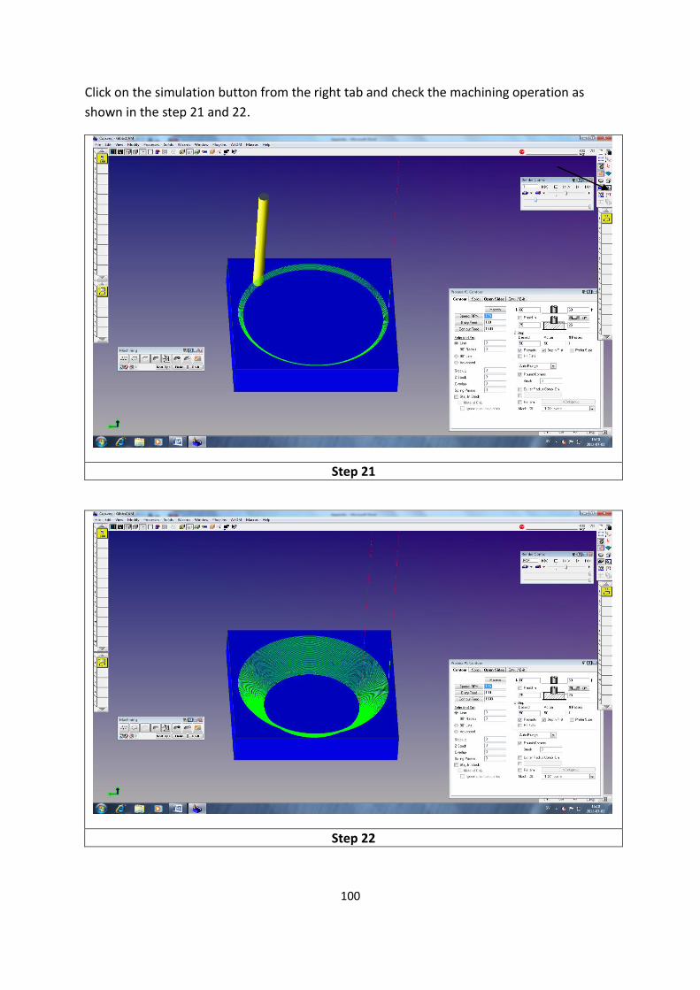
100
Click on the simulation button from the right tab and check the machining operation as
shown in the step 21 and 22.
Step 21
Step 22

101
The final tool path as shown in the step 23
Step 23
Top Related