


Languages
Pages
Legal


161
Simulation of wind-driven ventilation in an urban underground station
Roberta Ansuini – Università Politecnica delle Marche, Ancona, Italia
Alberto Giretti – Università Politecnica delle Marche, Ancona, Italia
Roberto Larghetti – Università Politecnica delle Marche, Ancona, Italia
Costanzo Di Perna – Università Politecnica delle Marche, Ancona, Italia
Abstract
Sustainable Energy Management for Underground
Stations (Seam4us) is a European research project aimed
at developing adaptive control technologies to reduce
energy consumption in subway stations. The research
work is developed through a pilot subway station, the
Passeig de Gracia – Line 3 station, in Barcelona, Spain.
The entrances to the subway station are located along
Passeig de Gracia, one of Barcelona’s main avenues. In
this type of location, evaluating the effects of wind in
terms of underground ventilation, requires profound
investigation. In the perspective of the Seam4us project,
wind-driven ventilation must be known a priori in order
to evaluate natural ventilation potentials and patterns
related to wind-driven ventilation, and to compute wind
pressure coefficients used in a synthetic lumped
parameter model that is the training model for the control
policy. In this perspective, an urban canyon model was
built in a commercial CFD simulation environment.
Different CFD modeling steps and simulations were
faced in order to achieve reliable data, which was then
compared with experimental data retrieved from an on-
site survey. The results are discussed in the present
paper.
1. Introduction
Evaluating the effects of wind, in terms of building
ventilation, calls for profound investigation.
Factors due to wind forces affecting the ventilation
rate inside buildings include average speed,
prevailing direction, seasonal and daily variation
in speed and direction, and local obstructions such
as nearby buildings, hills, trees, and shrubbery
(Liddament, 1988).
(Horan et al., 2008) showed that assuming external
airflow data on the basis of a single, mean wind
speed, and an associated prevailing wind direction,
could result in significant variations in ventilation
rates, and in comfort conditions when other,
external wind conditions prevail. Furthermore, the
relationship between wind direction and air
change rate proved to be non-linear in many cases.
To model the effects of airflow in buildings, wind
speed and direction frequency data are necessary.
Generally, the turbulence or gustiness of
approaching wind, and the unsteady character of
separated flows, cause the fluctuation of surface
pressures. (ASHRAE, 2005) states that although
peak pressures are important with regards to
structural loads, mean values are more appropriate
for computing infiltration and ventilation rates. It
considers time-averaged values for pressure, with
the shortest averaging period of about 600s
(approximately, the shortest time period
considered to be a “steady-state” condition when
considering atmospheric winds) and the longest
3600s. Instantaneous pressures may vary
significantly above and below these averages. Peak
pressures even doubled or tripled their mean
values.
Furthermore, urban environments have drawbacks
in terms of the application of natural ventilation:
lower wind speed and higher temperatures due to
the effect of urban heat island, noise and pollution
(Ghiaus et al., 2006). The meteorological models
currently available usually give the wind,
temperature, and sky cover on a fictitious surface,
usually measured at 10m above ground level, and
on a several kilometre grid, approximately. These
values need to be changed as a function of the

Roberta Ansuini, Alberto Giretti, Roberto Larghetti,Costanzo Di Perna
162
urban environment (Ghiaus et al., 2003) in order to
be used for estimating natural ventilation airflow
due to wind pressure and stack effect. An urban
canyon is an urban environment artefact similar to
a natural canyon. It is characterized by streets
cutting through dense blocks of structures -
generally heights (Santamouris et al. 1999). Airflow
in street canyons has much lower values as
compared to undisturbed wind. Lower wind
velocity means reduced wind pressure on building
facades and less effective cross ventilation.
Experimental evaluation of the reduction of airflow
rate in single-sided and cross-ventilated buildings
in 10 urban canyons in Athens (Geros et al., 1999)
showed that airflow rate might be reduced by 90%.
Knowledge of the wind speed in urban canyons is
a required input for estimating the natural
ventilation potential of urban buildings, as well as
thermal comfort in open areas. Wind flow inside
canyons is driven and determined by the
interaction of the flow field above buildings and
the uniqueness of local effects such as topography,
building geometry and dimensions, streets, traffic,
and other local features.
Three approaches can be used to acquire data
regarding urban canyon wind flows:
Measurements on site: This process requires
months for the acquisition of data using
anemometers and important instrument set-ups;
Wind tunnel tests: A slightly faster approach, but
also a more expensive one, especially in terms of
the construction of the neighbourhood and
buildings’ physical model ;
Computational Fluid Dynamics (CFD): a faster and
cheaper approach, producing much more detailed
information but also more “uncertain” data.
While the use of CFD in engineering practice is
becoming a well-established procedure in indoor
applications, they are used considerably less in
outdoor applications; although numerical
modeling with CFD is becoming a quite common
approach for urban wind simulation. Indeed, CFD
models can provide detailed information regarding
relevant flow variables in the whole calculation
domain (“whole-flow field data”), under well-
controlled conditions and without similarity
constraints. Furthermore, CFD models can avoid
some of the limitations found in other models.
Even so, numerical and physical modeling errors
need to be assessed by detailed verification and
validation studies (Franke et al., 2007).
2. Urban Canyon Model in Seam4us
The development of a new class of energy control
systems for underground public environments is
one of the main objectives of the EU-funded R&D
project called Sustainable Energy Management for
Underground Stations (SEAM4US). The project
aims at developing a fully featured pilot system, in
Barcelona’s “Passeig de Gracia” subway station, for
the dynamic control of energy consumption,
capable of setting up internal environments
opportunistically and optimally, based on external
environment forecasts, according to energy
efficiency, comfort and regulation requirements.
The development of this class of advanced control
system requires a robust modeling framework
(Giretti et al., 2012) as the models are needed both
for being embedded in the control system and for
supporting the whole system design, especially the
monitoring sensor network.
In this perspective, the model-engineering
framework in SEAM4US is hybrid (Ansuini et al.,
2012) as it includes different types of models (FEM,
Lumped Parameter, and Probabilistic Models) and
diverse processes (heat transfer, fluid dynamics,
pollutant transport, lighting) at various scales
(meteorological weather, local weather, indoor
environments).
A very critical point is modelling the effect of
meteorological weather conditions inside stations.
Every subway station has numerous entrances,
thus a local weather station deployed in each of the
entrances is economically unsustainable. The idea
currently being developed uses a third party
weather forecasting service for gathering
information pertaining to the climatic conditions
within the city, and includes knowledge about
local conditions related to a specific urban context
as well as the entrances’ geometric features, in
embedded models. Thus, only one local weather
station is deployed in each station (as part of the
monitoring system) and used to check the weather
model in real-time.

Simulation of wind-driven ventilation in an urban underground station
163
Two types of models are required:
A weather model including the third party weather
service data and correlation among the
aforementioned data and locally measured data,
A general model of the energetic behaviour of the
station building, including the effect of external
weather, using a thermal coefficient and a set of
specifically computed Wind Pressure Coefficients
(Costola et al., 2009).
The development of both the models requires the
initial development of an urban canyon model.
This study presents the urban canyon model
developed for the SEAM4US pilot station, located
in Passeig de Gracia (PdG), Barcelona. Only a very
preliminary set of experimental data is available to
date, gathered during a two-day environmental
survey. These data are used in this study for
performing a preliminary calibration of the
developed CFD models and for defining a
methodology for selecting real-time experimental
data to be used in the weather model check.
3. Model development
3.1 Model settings
Accuracy is an important matter of concern when
using CFD for modeling urban blocks. Care is
required in the geometrical implementation of the
model, in grid generation and in selecting proper
solution strategies (Franke et al., 2007).
An outdoor urban canyon model was developed. It
encompasses the eight city blocks surrounding the
station entrances. In order to be used to determine
the velocity maps at the station entrances and
inside the station, the model also contains the
underground environments (Fig. 2).
Critical parameters were determined on the basis
of the literature (Franke et al., 2004). Specifically, it
emerged that the main decisions to be taken
regarded:
the general modeling approach (what was
to be modelled) ;
the computational domain;
insertion of the “boundary layer” ;
roughness of the material;
geometrical detail level.
Regarding the modeling approach, according to
(Franke et al., 2007), the final decision was to
model only the volumes of fluid (air) included
among the buildings and inside the station. Hence,
a domain composed of a single material was
inserted in the calculation software. Thus, all other
components that really exist were excluded in
order to obtain a simple geometry, capable of
reducing the computational charges.
Fig. 1 – Urban Region around PdG modelled
The computational domain consists in a box
measuring 2 km in length, 1.5 km in width and 220
m in height, where 20 m was the height of the
ground and 200 m that of the air. The PdG
underground station has eight entrances. It
measures 630 m in length along the homonymous
street and measures about 190 m in width in the
perpendicular direction. Two different regions are
defined in the computational domain (Fig. 1), a
central box containing the real obstacles with their
geometric shape and with a level of detail
characterized by greater precision close to the
points of interest, and a less detailed peripheral
zone.
The boundary layer has not been included so far,
because the width of the computational domain
would generate a computationally uncontrollable
number of degrees of freedom.
The roughness of the boundary material is
considered, however, editing the speed of friction
in the conduit. In particular, the B parameter
(Comsol, 2011) is set to the value -3. This value was
obtained calibrating internal models of the station
with other data gathered in the station corridors
during the preliminary survey.
Regarding the level of geometrical detail of the

Roberta Ansuini, Alberto Giretti, Roberto Larghetti,Costanzo Di Perna
164
representation, the buildings were considered with
clean surfaces and street furniture in the area
surrounding the entrances was included (Fig.2).
Fig. 2 – Detail of the model in the area surrounding the station
entrances
3.2 Boundary Conditions
Four different types of boundary conditions were
used (Fig. 3):
Slip condition, imposed on the sky of the
computational domain to avoid viscous
phenomena on the wall and assuming the
continuity of the fluid;
Wall function condition, imposed on the surfaces
of the air volume adjacent to a solid;
Inlet condition, applying a velocity profile to the
surface of the air box the wind is arriving from;
Outlet condition “Pressure Zero”, which considers
a pressure profile constant and equal to 0 on the
surface, simulating the passage of flow from a tube
that represents our computational domain in an
undisturbed environment, as occurs in the surface
opposite the inlet.
Fig. 3 – Boundary Conditions on different Surfaces
Two types of inlet conditions were considered,
each required a different simulation for each
model, depending on the velocity profile. Of
course, in reality, the wind speed profile along the
atmosphere height has a logarithmic trend, but this
profile is not fully known, as it will be measured
only in one point. This point corresponds to the
meteorological weather station. Thus, the
definition of the logarithmic profile could include
an error related to its trend. On the other hand, the
linear profile (according to (Franke, 2004)) can
ensure the development of a logarithmic profile
due to friction with the ground if used soundly,
but the overall effect may be underestimated.
The two profiles considered so far are:
Linear WS(z) = WSMet
Logarithmic WS(z) = WSMet*(z/10)0.2.
Fig. 4 – Linear and Logarithmic Speed Profile in relation to the
experimental WSMet
3.3 Model definition by wind direction
In order to apply the inlet boundary condition
efficiently, the surface in which it is applied must
be normal to the wind vector direction. Thus,
different models were developed for each of the
sixteen, main wind directions, resulting in eight
different geometrical models (opposite wind
directions can use the same geometry).
3.4 Meshing
The results of the computation are strongly
dependent on the grid that used to discretize the
computational domain. In this case, two different
meshes were used for the two different
computational domains.
The discretization of the model is obtained by
means of a free form mesh grid (normally
tetrahedral), which varies in size according to the
degree of accuracy to be obtained.
The CFD program used in this study allows two
types of meshes: one, based on the general physical

Simulation of wind-driven ventilation in an urban underground station
165
behaviour that does not require a very accurate
grid (the default size is then larger), and another,
based on the fluid dynamic models’ degree of
accuracy (the default size is smaller) (Fig. 5). The
two subsets include various grid default sizes
ranging from an extremely detailed grid for the
central region (with dimensions sub-centimetre),
while the extreme regions are characterized by a
much higher minimum dimension mesh (order of
50 m). In this modeling case, a grid size in the
order of 30 meters in the peripheral areas and a
centimetric grid size, with fluid-dynamic
characteristics in the central region, is deemed
necessary. Table 1 gives a summary of the meshing
details.
Fig. 5 – Model mesh
Ma
x e
lem
. si
ze (
m)
Min
ele
m.
siz
e (m
)
Ma
x e
lem
. g
row
. ra
te
Re
sol.
of
curv
atu
re
Re
sol.
of
na
rro
w r
eg
ion
s
Central 20 0.05 1.5 0.6 0.5
Peripheral 69.5 2 1.2 0.7 0.6
Table 1 – Meshing details
In the post-processing phase, the quality of the
mesh was checked, confirming that the variable
“wall lift off” δw was equal to 11.06 on most of the
walls, guaranteeing a good accuracy (Comsol,
2011).
In fact, the wall functions in COMSOL are such
that the computational domain is assumed to start
at distance δw from the wall, which is the distance
from the wall where the logarithmic layer would
meet the viscous sub-layer if there were no buffer
layer in between.
3.5 Model solving
The simulations were carried out by means of
COMSOL Multi-physics 4.3, 3D steady state
analysis (Comsol, 2012).
The Physical Equations used are those related to
the κ-ε Turbulence Model (Wilcox, 1998) in steady
Reynolds-averaged Navier-Stokes (RANS)
simulation, which is the commonly used method
(Yoshie et al., 2007).
4. Experimetnal data
An environmental survey in PdG station was
carried out on the 21st and 22nd of March 2012 to
retrieve a very preliminary snapshot of the pilot
station’s environmental behaviour.
A number of different types of data were collected,
including local weather data using a weather
station (WS3600 LaCrosse Technology) placed close
to the EN5 entrance (Fig. 6). The instrument has a
resolution of 0.1 m/s for WS and 22.5 deg for WD.
The data was acquired with a 1 minute time step
from 9:00 a.m. to 6:00 p.m. during the first day and
from 9:00 a.m. to 3:00 p.m. during the second one
(Fig. 7).
Fig. 6 – Local Weather Station during the survey
Fig. 7 – Original data acquired by the Local Weather Station
during the survey.

Roberta Ansuini, Alberto Giretti, Roberto Larghetti,Costanzo Di Perna
166
4.1 Calibration approach
For the calibration of the weather models, the
SEAM4US project uses two types of Wind
Measurement (Fig. 8):
Local Wind data, similar to that retrieved during
the preliminary survey, gathered from the Weather
Station placed in the entrance EN5;
Meteorological Wind data retrieved by a third
party weather service. The services considered so
far, for the city of Barcelona, use mainly data
gathered by the Barcelona El Prat Airport weather
station, situated at an altitude of 6m, free field.
This data was also used for the preliminary
calibration.
Fig. 8 – Diagram of the relation between Meteorological and
Local Wind
4.2 Analysis of Meteorological Wind
Data
Meteorological wind data, corresponding to the
Local Weather Station’s measurement time-period,
was collected. The weather forecast services
considered provide 30 minute averaged data, thus,
19 records for the first day, and 17 records for the
second. Their distribution in terms of WD and WS
are shown in Figure 9.
4.3 Definition of the CFD model set
The data available was analysed and 22 boundary
conditions were identified on the basis of the
winds occurring. The related models were
developed and simulated.
Fig. 9 – Data about the Meteorological Wind related to the survey
period
4.4 Detailed analysis of local wind data
The critical part of the calibration process is then
the analysis of local wind data. Weather stations,
such as the one used in the survey, have a rather
low accuracy: ±10% (AmbientWeather, 2012) that
can increase to ±30% for WS < 1 m/s (Rossi, 2003).
Furthermore, in terms of WD, they give a result
even if WS=0 (no wind).
Hence, in the perspective of real-time
checking/calibration, the definition of a protocol
for defining data reliability is critical.
As the data are averaged for each half hour, 30
measures are expected for each interval. The
analysis used in this study aims at defining the
reliability of measures, depending on three
parameters:
Validity: that is, computing the number of
measures that are valid and correspondent to a
wind (WS>0). The interval set is defined valid if at
least 10 measures are valid;
Reliability: that is, computing the number of
measures corresponding to WS>1 m/s. The interval
set is defined reliable if the majority of the valid
measures are also reliable;
Direction Prevalence: that is, computing the
number of occurrences of each WD between the
valid measures. If the most frequent WD, in terms
of occurrence, has a number of measures greater
than one-third the number of valid measures, and
at least double of the number of the second WD
cases, in terms of occurrences, it can be considered
a prevalent direction (Fig. 10).
Fig. 10 – Example about the identification of Prevalent WD in a
half hour interval
Setting the reliability threshold to 1 m/s is related
to (Rossi, 2003) and can be considered plausible for
our case given that its effect inside the station is not
Dir 1 202.5(14) Dir 2 270 (4) Dir 1 270 (12) Dir 2 157.5 (10)
is 14>(24/3) ? YES is 14 >(2*4) ? YES is 12>(28/3) ? YES is 12 >(2*10) ? NO
10.30-11.00 _ NOT Prevalent WD
valid cases: 28valid cases: 24
11.30-12.00 _ Prevalent WD: 202.5
0
5
10
150/360
22.5
45
67.5
90
112.5
135
157.5
180
202.5
225
247.5
270
292.5
315
337.5
0
2
4
6
8
10
120/360
22.5
45
67.5
90
112.5
135
157.5
180
202.5
225
247.5
270
292.5
315
337.5

Simulation of wind-driven ventilation in an urban underground station
167
very relevant when the outdoor wind speed is low.
Based on these criteria, only reliable measures were
considered, hence, 17 half-hour intervals from the
survey data. For each interval, average WDLoc and
WSLoc were computed.
WDLoc was computed as the direction occurrence
weighted average of the valid WD measures,
paying particular attention to accounting properly
the cases where the measures were around the
0/360 angle.
WSLoc was computed differently depending on
whether or not there was a single, prevailing wind
direction: if a prevalent direction existed, the
average, prevalent direction, WS was used.
However, if a prevalent wind direction did not
exist, the weighted average of all the average WS
for each direction was used.
5. Results and discussion
5.1 Simulation Results
The whole CDF model set identified was
developed and simulated. A line of plotting points
was defined in each model, centred on the actual
position of the Weather Station during the survey
(Fig. 11).
Fig. 11 – Plot points around the weather station
Table 2 reports the simulation results related to the
reliable data of Local Wind, in both inlet conditions
cases: linear (lin) and logarithmic (log) speed
profile.
The analysis of the simulation performance was
performed in terms of WD and WS.
In terms of WD, the results are very good as the
mean errors obtained are ±27.98 (lin) and ± 27.30
(log). Recalling that the weather station precision
was ±22.5 degrees, the results appropriateness is
confirmed. In percentage terms, the relative errors
are ±14.9% and ±14.3%, which, considered in
reference to 360 degrees, are ±7.8% and ± 7.6%.
In terms of WS, the mean errors obtained are ±0.62
m/s (lin) and ± 0.41 m/s (log), corresponding to
relative percentage errors of 36.8% and 26.8%.
time WDS_Li
n
WSS_Lin WDS_Lo WSS_Log
9.30-10.00 216.58 0.92 221.54 1.90
10.00-10.30 216.31 0.82 221.13 1.69
10.30-11.00 216.31 0.82 221.13 1.69
11.30-12.00 215.40 0.60 219.58 1.20
12.00-12.30 215.40 0.60 219.58 1.20
12.30-13.00 215.40 0.60 219.58 1.20
13.00-13.30 185.00 0.84 187.88 1.10
13.30-14.00 185.00 0.84 187.88 1.10
14.30-15.00 221.23 0.96 223.21 1.66
15.30-16.00 215.81 0.95 221.54 2.08
16.00-16.30 215.81 0.95 221.54 2.08
17.00-17.30 225.89 1.26 226.61 2.05
17.30-18.00 216.58 0.92 221.54 1.90
12.30-13.00 187.96 0.50 187.85 0.64
13.30-14.00 145.22 0.87 136.80 1.12
14.00-14.30 187.96 0.50 187.85 0.64
14.30-15.00 187.96 0.50 187.85 0.64
Table 2 – Simulation Results
5.2 Discussion
Figures 12-15 support a detailed analysis of the
results.
Figure 12 represents WD and WS with the results
ordered by WDMet.
It emerges that the cases related to directions 80,
180 and 190 have recurrent problems, in terms of
both WS and WD. In particular, the WS graph (Fig.
12b) shows that this problem is not related to the
inlet condition and it should be related to the
model. This behaviour has a physical explanation,
as these directions are the most oblique to the city
block grids (and to the canyon) as showed in
Figure 13.
Roberta Ansuini, Alberto Giretti, Roberto Larghetti,Costanzo Di Perna
168
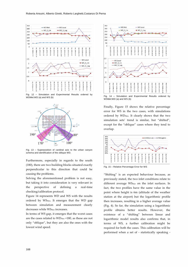
Fig. 12 – Simulation and Experimental Results ordered by
WDMet:WD (a) and WS (b)
Fig. 13 – Superposition of cardinal axis to the urban canyon
schema and identification of the oblique WD.
Furthermore, especially in regards to the south
(180), there are two building blocks situated exactly
perpendicular to this direction that could be
causing the problems.
Solving the aforementioned problem is not easy,
but taking it into consideration is very relevant in
the perspective of defining a real-time
checking/calibration protocol.
Figure 14 represents WD and WS with the results
ordered by WSMet. It emerges that the WD gap
between simulation and measurement clearly
decreases while WSMet increases.
In terms of WS gap, it emerges that the worst cases
are the cases related to WDMet =180, as these are not
only “oblique”, but they are also the ones with the
lowest wind speed.
Fig. 14 – Simulation and Experimental Results ordered by
WSMet:WD (a) and WS (b)
Finally, Figure 15 shows the relative percentage
error for WS in the two cases, with simulations
ordered by WDMet. It clearly shows that the two
simulation sets’ trend is similar, but “shifted”,
except for the “oblique” cases where they tend to
overlap.
Fig. 15 – Relative Percentage Error for WS
“Shifting” is an expected behaviour because, as
previously stated, the two inlet conditions relate to
different average WSMet on the inlet surfaces. In
fact, the two profiles have the same value in the
point where height is 6m (altitude of the weather
station at the airport) but the logarithmic profile
then increases, resulting in a higher average value
(Fig. 4). So far, the simulation using a logarithmic
profile obtains better results. However, the
existence of a “shifting” between linear and
logarithmic model results also confirms that, in
terms of WS, a further calibration might be
required for both the cases. This calibration will be
performed when a set of - statistically speaking -

Simulation of wind-driven ventilation in an urban underground station
169
more reliable experimental data is available.
It also emerges that there is still a “fluctuation” of
the model’s performance in terms of WS. In our
opinion, this could be related to two main aspects.
The first is “structural” in the process, and it is
related to the action of “averaging” the wind.
Averaging the wind speed, and defining the
prevalent wind direction for both the two
locations, is a very critical step in this process. So
far, two different subjects conduct this step
autonomously (the airport weather service and the
authors) for two different sets of data. This
procedure will be the same during the real-time
phase, although, a deeper investigation regarding
the averaging interval length could be useful. The
30-minute length chosen so far is related to the
availability of real-time data from the
meteorological weather services. The averaging
interval could be modified to 10 minutes, if more
detailed data from some weather service is made
available.
The second aspect is the possible inaccuracy of
some measurements in both the two weather
stations (airport and canyon) during the survey. So
far, the preliminary calibration is based on 17 cases,
meaning possible “wrong” measures (not easy to
be identified, especially if they are related to the
weather station at the airport, not directly
managed by the authors) highly affect overall
performance. This aspect will be investigated
further using statistical correlations when more
experimental data is available from the local
weather station. Thus, the weight of possible
“anomalous” cases will be reduced statistically.
6. Conclusion
This paper presents the development and
preliminary calibration of a CFD urban canyon
model used in the EU funded project SEAM4US.
The model aims at representing the relation
between Meteorological Wind and local winds near
subway station entrances; in this case, the pilot
case used is the Passeig de Gracia subway station
in Barcelona.
The preliminary calibration is based on a small
experimental data set, thus the results will have to
be updated with a larger set of data. However, the
preliminary results showed a very good
convergence in terms of WD, with an average error
of 27.30 deg, close to the precision of the
instrument 22.5 deg. In terms of WS, the model
would benefit from a further calibration (average
error 0.41 m/s), which will be performed once more
experimental data is available.
Furthermore, the paper discusses the data in the
perspective of defining a protocol for the real-time
comparison of experimental data concerning
Meteorological and Local Wind, and simulation
results, as this operation will have to be performed
by the SEAM4US Control System.
7. Nomenclature
Symbols
WS Wind Speed (m/s)
WD Wind Direction (degree)
Subscripts/Superscripts
Loc Local (in the urban canyon weather
station)
Met Meteorological (in the airport weather
station)
S_Lin Simulated/Linear Inlet Condition
S_Log Simulated/Logarithmic Inlet
Condition
References
AmbientWeather.http://ambientweather.wikispace
s.com/Weather+Station+Comparison+Guide
Ansuini R., Larghetti R., Vaccarini M., Carbonari
A., Giretti A., Ruffini S., Guo H., Lau S.L.,
“Hybrid Modeling for Energy Saving in
Subway Stations”, in proceedings of: BSO12 -
Building Simulation and Optimization 2012,
Loughborough, UK, September 10-11, 2012
ASHRAE 2005, Handbook Fundamentals, Atlanta.
Comsol, 2011. CFD Module User’s Guide, p.162.
Comsol, 2012. COMSOL Multiphysics Version 4.3.
Costola D, Blocken B, Hensen JLM, 2009. Overview
of pressure coefficient data in building energy
simulation and airflow network programs.
Build Environ 2009, 44: 2027-2036.

Roberta Ansuini, Alberto Giretti, Roberto Larghetti,Costanzo Di Perna
170
Franke, J., Hirsch, C., Jensen, A.G., Krüs, H.,
Schatzmann, M., Westbury, P., Miles, S., Wisse,
J., Wright, N., 2004. Recommendations on the
use of CFD in wind engineering. In: van Beeck,
J.P.A.J. (Ed.), Proc.of the International
Conference on Urban Wind Engineering and
Building Aerodynamics. COST Action C14.,
Sint-Genesius-Rode, Belgium.
Franke J, Hellsten A., Schlünzen H., Carissimo
B.,2007. Best practice guideline for the CFD
simulation of flows in the urban environment.
COST Office Brussels, ISBN 3-00-018312-4.
Geros V, Santamouris M, Tsangrassoulis A,
Guarracino G., 1999. Experimental evaluation
of night ventilation phenomena. Energy and
Buildings 1999;29:141–54.
Ghiaus C, Allard F., 2003. Natural ventilation in an
urban context. In: Santamouris M, editor. Solar
thermal technologies for buildings. London:
James and James; 2003. p. 116–39.
Ghiaus C., Allard F., Santamouris M., Georgakis
C., Nicol F., 2006. Urban environment influence
on natural ventilation potential. Building and
Environment 41 (2006) 395–406.
Giretti A., Lemma M., Vaccarini M., Ansuini R.,
Larghetti R., Ruffini S., “Environmental
Modelling for the Optimal Energy Control of
Subway Stations”, Gerontechnology 11(2):168,
2012.
Horan J.M., Finn D.P., 2008. Sensitivity of air
change rates in a naturally ventilated atrium
space subject to variations in external wind
speed and direction. Energy and Buildings 40
(2008) 1577–1585.
Liddament, M.W. 1988. The calculation of wind
effect on ventilation. ASHRAE Transactions
94(2):1645-1660.
Rossi N., 2003. Manuale del Termotecnico. Hoepli.
Santamouris M., Papanikolaou N., Koronakis I.,
Livada I., Asimakopoulos D., 1999. Thermal
and airflow characteristics in a deep pedestrian
canyon under hot weather conditions.
Atmospheric Environment 33 (1999) 4503:4521.
Wilcox, D.C. 1998. Turbulence Modeling for CFD,
2nd ed., DCW Industries, 1998.
Yoshie, R., Mochida, A., Tominaga, Y., Kataoka,
H.,Harimoto, K., Nozu, T., Shirasawa, T. 2007.
Cooperative project for CFD prediction of
pedestrian wind environment in the
Architectural Institute of Japan. J. Wind Eng.
Ind. Aerodyn. 95(9-11): 1551-1578.
Top Related