Download - Simulation Environment for UAV Fault Tolerant Autonomous Control … - Simulation Environ… · · 2013-12-29Simulation Environment for UAV Fault Tolerant ... manual or autonomous

Columbia International Publishing Journal of Modeling, Simulation, Identification, and Control (2013) Vol. 1 No. 4 pp. 164-195 doi:10.7726/jmsic.2013.1011

Research Article

______________________________________________________________________________________________________________________________ *Corresponding e-mail: [email protected] 1 West Virginia University, Morgantown, West Virginia 2 Embry-Riddle Aeronautical University, Daytona Beach, Florida 3 Instituto Politécnico Nacional, Mexico

164

Simulation Environment for UAV Fault Tolerant Autonomous Control Laws Development

Mario G. Perhinschi1*, Brenton Wilburn1, Jennifer Wilburn1, Hever Moncayo2, and Ondrej Karas3

Received 27 June 2013; Published online 26 October 2013 © The author(s) 2013. Published with open access at www.uscip.us

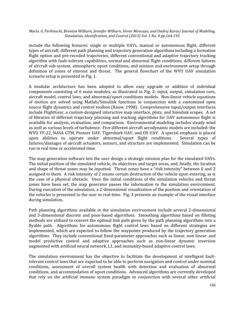
Abstract This paper presents a Matlab/Simulink simulation environment developed at West Virginia University to facilitate the design, testing, and analysis of fault-tolerant control laws for autonomous operation of unmanned aerial vehicles. Custom map generation software allows the user to setup the mission scenario by defining threat zones, obstacles, and points of interest. FlightGear provides vehicle and environment visualization. Maximum portability, flexibility, and extension capability are ensured through a modular structure including libraries of aircraft models, path planning algorithms, and trajectory tracking algorithms. Models for environmental upset conditions and aircraft sub-system failure/damage, including GPS, are implemented allowing the investigation of a variety of abnormal flight conditions. Several adaptive trajectory tracking algorithms with significant fault-tolerant potential are available. A set of comprehensive performance metrics based on tracking errors and control activity are computed and provided to the user for control laws performance analysis and comparison. The versatility and utility of the simulation environment is illustrated through example simulation results at normal and abnormal flight conditions. Keywords: unmanned aerial vehicles, aircraft modeling and simulation, fault-tolerant control

1. Introduction The use of unmanned aerial vehicles (UAVs) is expected to increase exponentially in the near future (Anon., 2010a; Anon., 2010b). As their operational capabilities diversify, there is a perceived need for a significant increase in their level of performance, reliability, effectiveness, and efficiency (Anon., 2009a). Critical issues such as operation safety, integration within the national airspace, functionality at both normal and abnormal/upset conditions, operational flexibility, optimality, and adaptation are all defining attributes of autonomy. The need for increased complexity missions and high levels of autonomy requires current and future UAV designs to become progressively more sophisticated and complex featuring on-board intelligence at different levels with the ability to

Mario. G. Perhinschi, Brenton Wilburn, Jennifer Wilburn, Hever Moncayo, and Ondrej Karas/ Journal of Modeling, Simulation, Identification, and Control (2013) Vol. 1 No. 4 pp.164-195

165

perform timely status determination, decision making, and adaptive navigation and control. The design process of systems with such challenging objectives needs the support of adequate simulation tools at all levels and phases (Perhinschi et al., 2010a). Typically, the development of modeling and simulation tools for UAVs, more advanced than just mathematical models for control system design (Jodeh et al., 2006), have been focused primarily on specific and limited aspects of vehicle dynamics and control at nominal conditions such as cooperative control (Rasmussen et al., 2002; Stevenson et al., 2007), multiple vehicle operation (Kim et al., 2007), human operator-vehicle interaction and training (De Crescenzio et al., 2007; Freedy et al., Annon., 2009b), and evaluation of control laws through hardware-in-the-loop simulations (Mueller, 2007). Commercially available flight simulation packages have also been customized and used for limited-scope UAV analysis (Craighead et al., 2007). For example, FlightGear (Annon., 2012a) and X-Plane (Annon., 2012b) are successful multi-purpose commercial simulators, which feature detailed graphics and numerous aircraft models; however, they have minimal provisions for autonomous flight for the design and research-oriented user. Larger scale efforts have focused on the general evaluation, integration, training, and interoperability of UAVs within complex systems (Clark et al., 1999; Twesme et al., 2003; Sardella and High, 2000). Although the importance of safety and robustness under abnormal/upset conditions is acknowledged (Williams, 2006), research efforts for the development of UAV autonomous flight control laws that possess significant fault-tolerant capabilities and the supporting simulation tools are still limited (Rago et al., 1998; Schaefer et al., 2000; Magrabi and Gibbens, 2000; Perhinschi et al., 2004a). There is no publicly available software, specifically adapted to UAV trajectory planning algorithm and autonomous flight control system design that would simulate flight dynamics in such detail to include a large variety of aircraft sub-system failures. In this paper, the development at West Virginia University (WVU) of an integrated simulation environment for the design, testing, demonstration, and analysis of algorithms for UAV autonomous flight with emphasis on accommodation of abnormal/upset conditions is presented. The paper is organized as follows. The general architecture of the WVU UAV simulation environment is presented in Section 2. The input and output modules including the various graphical user interfaces, as well as the general simulation nucleus are described in Sections 3. The aircraft aerodynamic models and the abnormal conditions module are presented in Sections 4 and 5, respectively. Section 6 provides a description of the control laws module including outlines of the path planning and trajectory generation algorithms, trajectory tracking algorithms, and the on-board intelligence capabilities. Section 7 includes simulation results at normal and abnormal flight conditions to illustrate the versatility and utility of the simulation environment. Finally, some conclusions are summarized in Section 8, followed by acknowledgements and a bibliographical list.

2. General Architecture of the Simulation Environment The WVU UAV simulation environment for fault-tolerant autonomous control laws design and testing is developed in Matlab/Simulink for maximum portability and flexibility, interfaced with FlightGear (Anon., 2012a) for aircraft and environment visualization. It includes customized map generation and visual feedback environment created in C#. The simulation scenario can be setup to


166

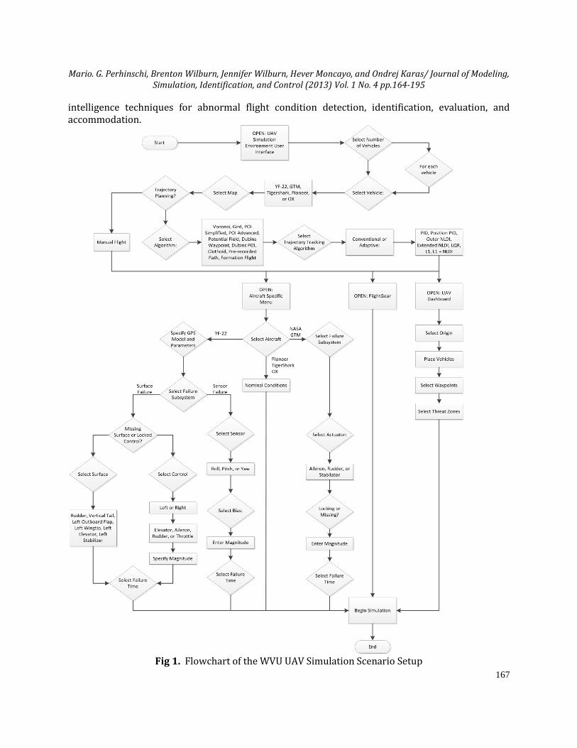
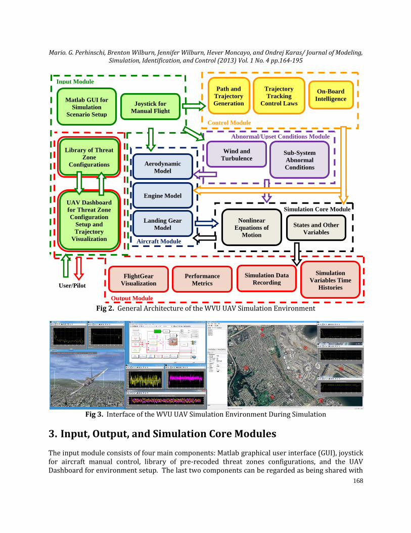
include the following features: single or multiple UAVs, manual or autonomous flight, different types of aircraft, different path planning and trajectory generation algorithms including a formation flight option and pre-recoded trajectories, different conventional and adaptive trajectory tracking algorithm with fault-tolerant capabilities, normal and abnormal flight conditions, different failures of aircraft sub-system, atmospheric upset conditions, and mission and environment setup through definition of zones of interest and threat. The general flowchart of the WVU UAV simulation scenario setup is presented in Fig. 1. A modular architecture has been adopted to allow easy upgrade or addition of individual components consisting of 6 main modules, as illustrated in Fig. 2: input, output, simulation core, aircraft model, control laws, and abnormal/upset conditions models. Non-linear vehicle equations of motion are solved using Matlab/Simulink functions in conjunction with a customized open source flight dynamics and control toolbox (Rauw, 1998). Comprehensive input/output interfaces include FlightGear, a custom-designed interactive map interface, plots, and Simulink scopes. A set of libraries of different trajectory planning and tracking algorithms for UAV autonomous flight is available for analysis, evaluation, and comparison. Environmental modeling includes steady wind as well as various levels of turbulence. Five different aircraft aerodynamic models are included: the WVU YF-22, NASA GTM, Pioneer UAV, Tigershark UAV, and OX UAV. A special emphasis is placed upon abilities to operate under abnormal/upset flight conditions. Several types of failures/damages of aircraft actuators, sensors, and structure are implemented. Simulation can be run in real time or accelerated time. The map generation software lets the user design a strategic mission plan for the simulated UAVs. The initial position of the simulated vehicle, its objectives and target areas, and, finally, the location and shape of threat zones may be inputted. Threat zones have a “risk intensity” between 0 and 2 assigned to them. A risk intensity of 2 means certain destruction of the vehicle upon entering, as is the case of a physical obstacle. Once the initial conditions of the simulation vehicles and threat zones have been set, the map generator passes the information to the simulation environment. During execution of the simulation, a 2-dimensional visualization of the position and orientation of the vehicles is presented to the user in real-time. Fig. 3 presents an example of the visual interface during simulation. Path planning algorithms available in the simulation environment include several 2-dimensional and 3-dimensional discrete and pose-based algorithms. Smoothing algorithms based on filleting methods are utilized to convert the optimal link path given by the path planning algorithms into a flyable path. Algorithms for autonomous flight control laws based on different strategies are implemented, which are expected to follow the waypoints produced by the trajectory generation algorithms. They include conventional fixed-parameter approaches such as linear, non-linear, and model predictive control and adaptive approaches such as non-linear dynamic inversion augmented with artificial neural network, L1, and immunity-based adaptive control laws. The simulation environment has the objective to facilitate the development of intelligent fault-tolerant control laws that are expected to be able to perform navigation and control under nominal conditions, assessment of overall system health with detection and evaluation of abnormal conditions, and accommodation of upset conditions. Advanced algorithms are currently developed that rely on the artificial immune system paradigm in conjunction with several other artificial


167

intelligence techniques for abnormal flight condition detection, identification, evaluation, and accommodation.

Fig 1. Flowchart of the WVU UAV Simulation Scenario Setup


168

Fig 2. General Architecture of the WVU UAV Simulation Environment

Fig 3. Interface of the WVU UAV Simulation Environment During Simulation

3. Input, Output, and Simulation Core Modules The input module consists of four main components: Matlab graphical user interface (GUI), joystick for aircraft manual control, library of pre-recoded threat zones configurations, and the UAV Dashboard for environment setup. The last two components can be regarded as being shared with

On-Board

Intelligence Matlab GUI for

Simulation

Scenario Setup

UAV Dashboard

for Threat Zone

Configuration

Setup and

Trajectory

Visualization

Joystick for

Manual Flight

Library of Threat

Zone

Configurations

FlightGear

Visualization

Performance

Metrics

Simulation Data

Recording

Simulation

Variables Time

Histories

Input Module

Output Module

Aircraft Module

User/Pilot

Aerodynamic

Model

Landing Gear

Model

Engine Model

Path and

Trajectory

Generation

Trajectory

Tracking

Control Laws

Control Module

Wind and

Turbulence Sub-System

Abnormal

Conditions

Abnormal/Upset Conditions Module

Nonlinear

Equations of

Motion

States and Other

Variables

Simulation Core Module


169

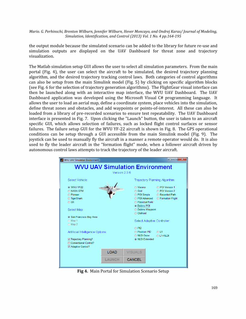
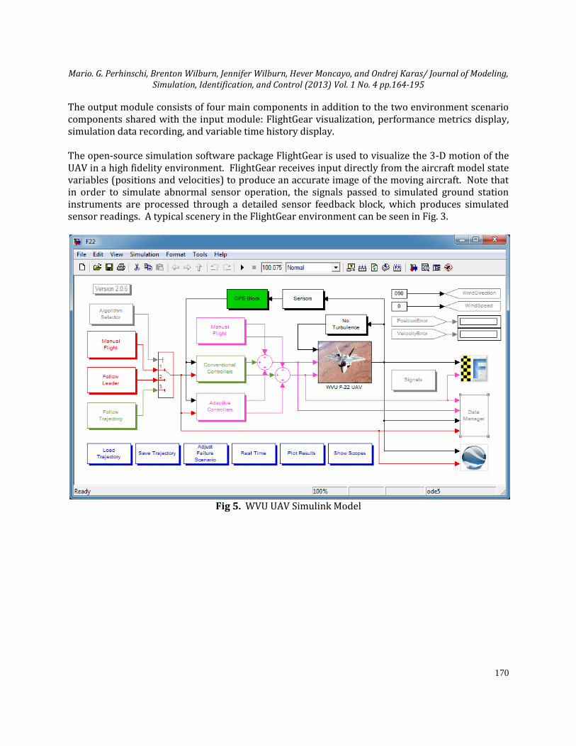
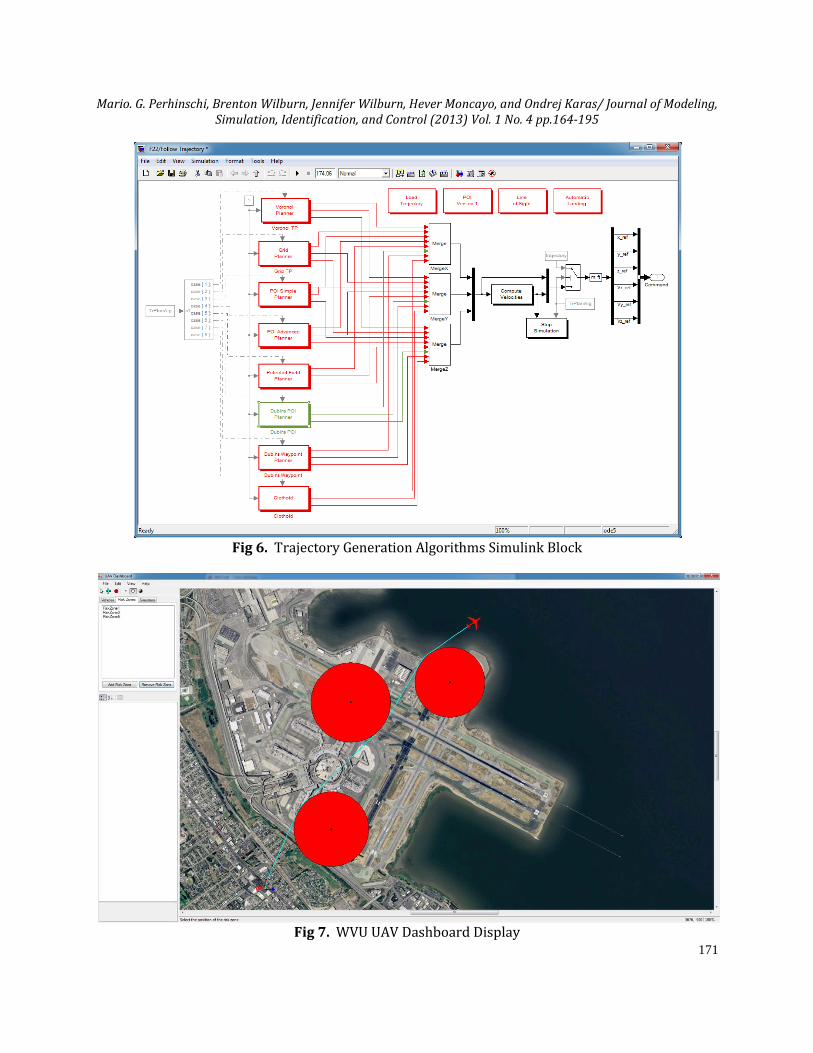
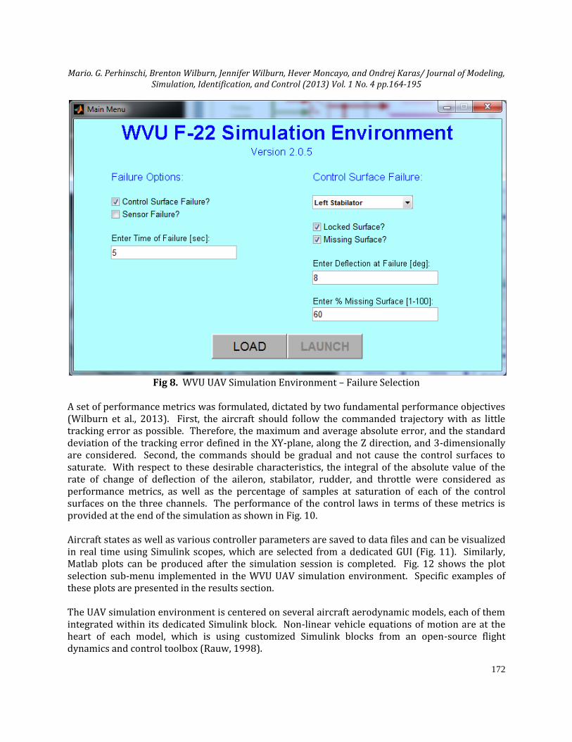
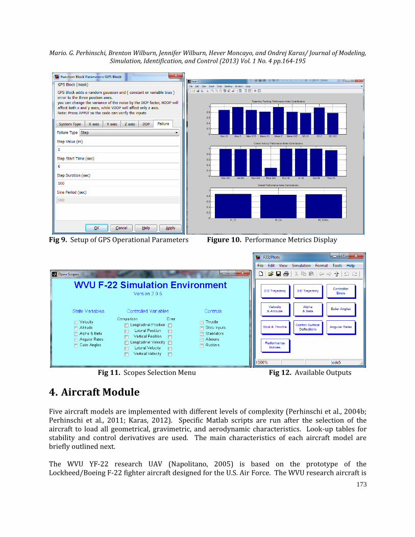
the output module because the simulated scenario can be added to the library for future re-use and simulation outputs are displayed on the UAV Dashboard for threat zone and trajectory visualization. The Matlab simulation setup GUI allows the user to select all simulation parameters. From the main portal (Fig. 4), the user can select the aircraft to be simulated, the desired trajectory planning algorithm, and the desired trajectory tracking control laws. Both categories of control algorithms can also be setup from the main Simulink model (Fig. 5) by clicking on specific algorithm blocks (see Fig. 6 for the selection of trajectory generation algorithms). The FlightGear visual interface can then be launched along with an interactive map interface, the WVU UAV Dashboard. The UAV Dashboard application was developed using the Microsoft Visual C# programming language. It allows the user to load an aerial map, define a coordinate system, place vehicles into the simulation, define threat zones and obstacles, and add waypoints or points-of-interest. All these can also be loaded from a library of pre-recorded scenarios to ensure test repeatability. The UAV Dashboard interface is presented in Fig. 7. Upon clicking the "Launch" button, the user is taken to an aircraft specific GUI, which allows selection of failures, such as locked flight control surfaces or sensor failures. The failure setup GUI for the WVU YF-22 aircraft is shown in Fig. 8. The GPS operational conditions can be setup through a GUI accessible from the main Simulink model (Fig. 9). The joystick can be used to manually fly the aircraft in a manner a remote operator would do. It is also used to fly the leader aircraft in the “formation flight” mode, when a follower aircraft driven by autonomous control laws attempts to track the trajectory of the leader aircraft.

Fig 4. Main Portal for Simulation Scenario Setup


170

The output module consists of four main components in addition to the two environment scenario components shared with the input module: FlightGear visualization, performance metrics display, simulation data recording, and variable time history display. The open-source simulation software package FlightGear is used to visualize the 3-D motion of the UAV in a high fidelity environment. FlightGear receives input directly from the aircraft model state variables (positions and velocities) to produce an accurate image of the moving aircraft. Note that in order to simulate abnormal sensor operation, the signals passed to simulated ground station instruments are processed through a detailed sensor feedback block, which produces simulated sensor readings. A typical scenery in the FlightGear environment can be seen in Fig. 3.

Fig 5. WVU UAV Simulink Model


171

Fig 6. Trajectory Generation Algorithms Simulink Block

Fig 7. WVU UAV Dashboard Display


172

Fig 8. WVU UAV Simulation Environment – Failure Selection

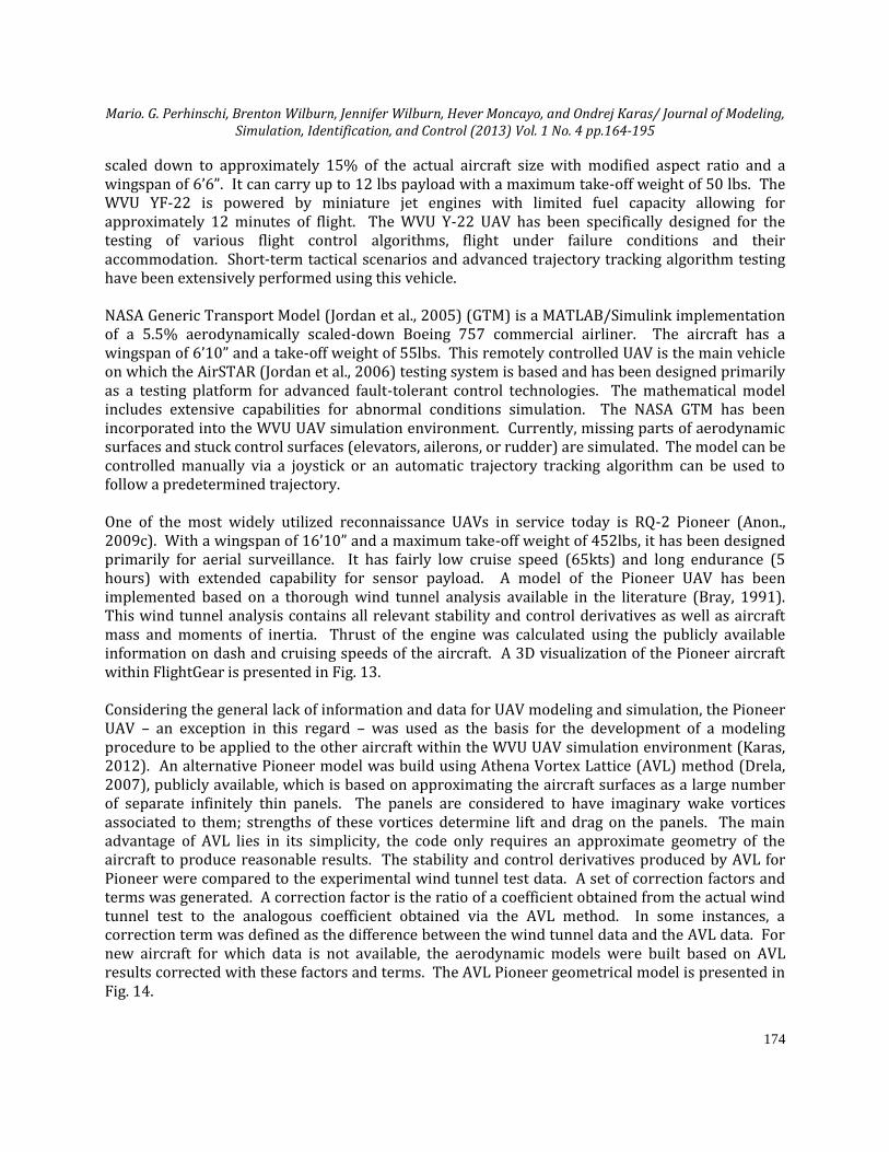
A set of performance metrics was formulated, dictated by two fundamental performance objectives (Wilburn et al., 2013). First, the aircraft should follow the commanded trajectory with as little tracking error as possible. Therefore, the maximum and average absolute error, and the standard deviation of the tracking error defined in the XY-plane, along the Z direction, and 3-dimensionally are considered. Second, the commands should be gradual and not cause the control surfaces to saturate. With respect to these desirable characteristics, the integral of the absolute value of the rate of change of deflection of the aileron, stabilator, rudder, and throttle were considered as performance metrics, as well as the percentage of samples at saturation of each of the control surfaces on the three channels. The performance of the control laws in terms of these metrics is provided at the end of the simulation as shown in Fig. 10. Aircraft states as well as various controller parameters are saved to data files and can be visualized in real time using Simulink scopes, which are selected from a dedicated GUI (Fig. 11). Similarly, Matlab plots can be produced after the simulation session is completed. Fig. 12 shows the plot selection sub-menu implemented in the WVU UAV simulation environment. Specific examples of these plots are presented in the results section. The UAV simulation environment is centered on several aircraft aerodynamic models, each of them integrated within its dedicated Simulink block. Non-linear vehicle equations of motion are at the heart of each model, which is using customized Simulink blocks from an open-source flight dynamics and control toolbox (Rauw, 1998).


173

Fig 9. Setup of GPS Operational Parameters Figure 10. Performance Metrics Display

Fig 11. Scopes Selection Menu Fig 12. Available Outputs

4. Aircraft Module Five aircraft models are implemented with different levels of complexity (Perhinschi et al., 2004b; Perhinschi et al., 2011; Karas, 2012). Specific Matlab scripts are run after the selection of the aircraft to load all geometrical, gravimetric, and aerodynamic characteristics. Look-up tables for stability and control derivatives are used. The main characteristics of each aircraft model are briefly outlined next. The WVU YF-22 research UAV (Napolitano, 2005) is based on the prototype of the Lockheed/Boeing F-22 fighter aircraft designed for the U.S. Air Force. The WVU research aircraft is


174

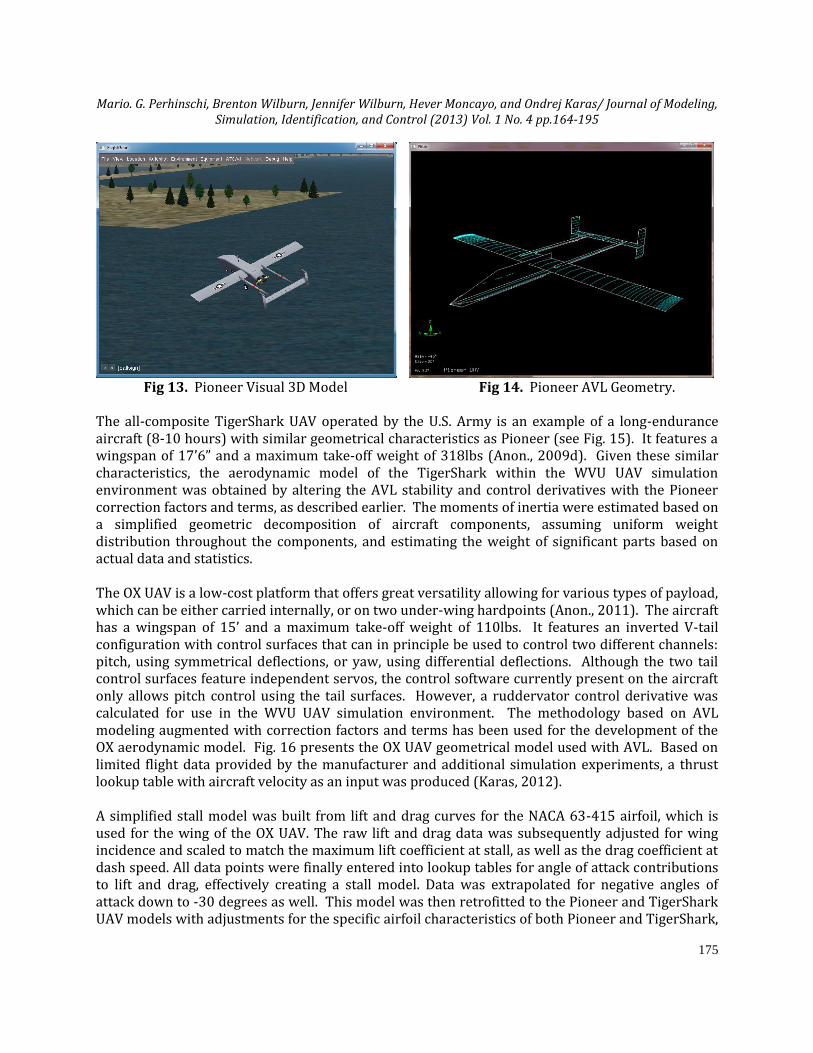
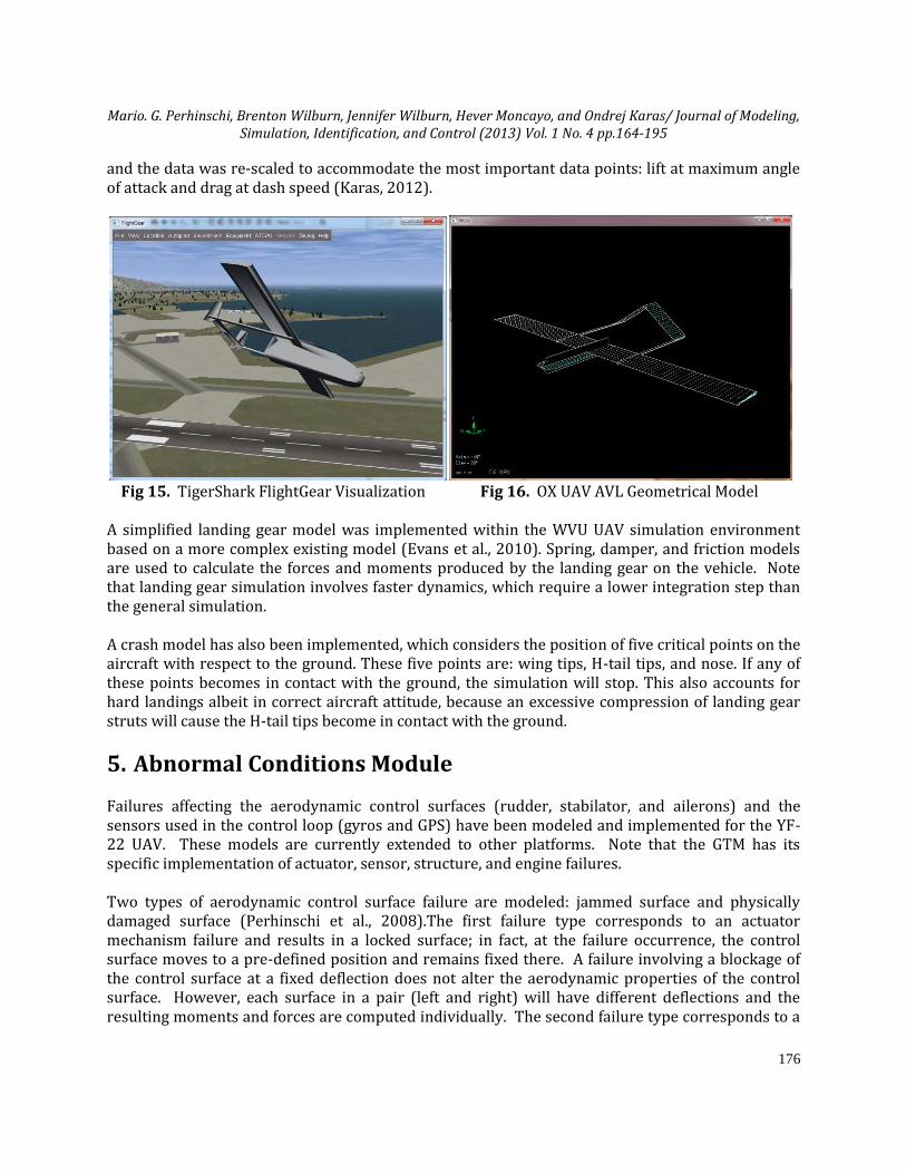
scaled down to approximately 15% of the actual aircraft size with modified aspect ratio and a wingspan of 6’6”. It can carry up to 12 lbs payload with a maximum take-off weight of 50 lbs. The WVU YF-22 is powered by miniature jet engines with limited fuel capacity allowing for approximately 12 minutes of flight. The WVU Y-22 UAV has been specifically designed for the testing of various flight control algorithms, flight under failure conditions and their accommodation. Short-term tactical scenarios and advanced trajectory tracking algorithm testing have been extensively performed using this vehicle. NASA Generic Transport Model (Jordan et al., 2005) (GTM) is a MATLAB/Simulink implementation of a 5.5% aerodynamically scaled-down Boeing 757 commercial airliner. The aircraft has a wingspan of 6’10” and a take-off weight of 55lbs. This remotely controlled UAV is the main vehicle on which the AirSTAR (Jordan et al., 2006) testing system is based and has been designed primarily as a testing platform for advanced fault-tolerant control technologies. The mathematical model includes extensive capabilities for abnormal conditions simulation. The NASA GTM has been incorporated into the WVU UAV simulation environment. Currently, missing parts of aerodynamic surfaces and stuck control surfaces (elevators, ailerons, or rudder) are simulated. The model can be controlled manually via a joystick or an automatic trajectory tracking algorithm can be used to follow a predetermined trajectory. One of the most widely utilized reconnaissance UAVs in service today is RQ-2 Pioneer (Anon., 2009c). With a wingspan of 16’10” and a maximum take-off weight of 452lbs, it has been designed primarily for aerial surveillance. It has fairly low cruise speed (65kts) and long endurance (5 hours) with extended capability for sensor payload. A model of the Pioneer UAV has been implemented based on a thorough wind tunnel analysis available in the literature (Bray, 1991). This wind tunnel analysis contains all relevant stability and control derivatives as well as aircraft mass and moments of inertia. Thrust of the engine was calculated using the publicly available information on dash and cruising speeds of the aircraft. A 3D visualization of the Pioneer aircraft within FlightGear is presented in Fig. 13. Considering the general lack of information and data for UAV modeling and simulation, the Pioneer UAV – an exception in this regard – was used as the basis for the development of a modeling procedure to be applied to the other aircraft within the WVU UAV simulation environment (Karas, 2012). An alternative Pioneer model was build using Athena Vortex Lattice (AVL) method (Drela, 2007), publicly available, which is based on approximating the aircraft surfaces as a large number of separate infinitely thin panels. The panels are considered to have imaginary wake vortices associated to them; strengths of these vortices determine lift and drag on the panels. The main advantage of AVL lies in its simplicity, the code only requires an approximate geometry of the aircraft to produce reasonable results. The stability and control derivatives produced by AVL for Pioneer were compared to the experimental wind tunnel test data. A set of correction factors and terms was generated. A correction factor is the ratio of a coefficient obtained from the actual wind tunnel test to the analogous coefficient obtained via the AVL method. In some instances, a correction term was defined as the difference between the wind tunnel data and the AVL data. For new aircraft for which data is not available, the aerodynamic models were built based on AVL results corrected with these factors and terms. The AVL Pioneer geometrical model is presented in Fig. 14.


175

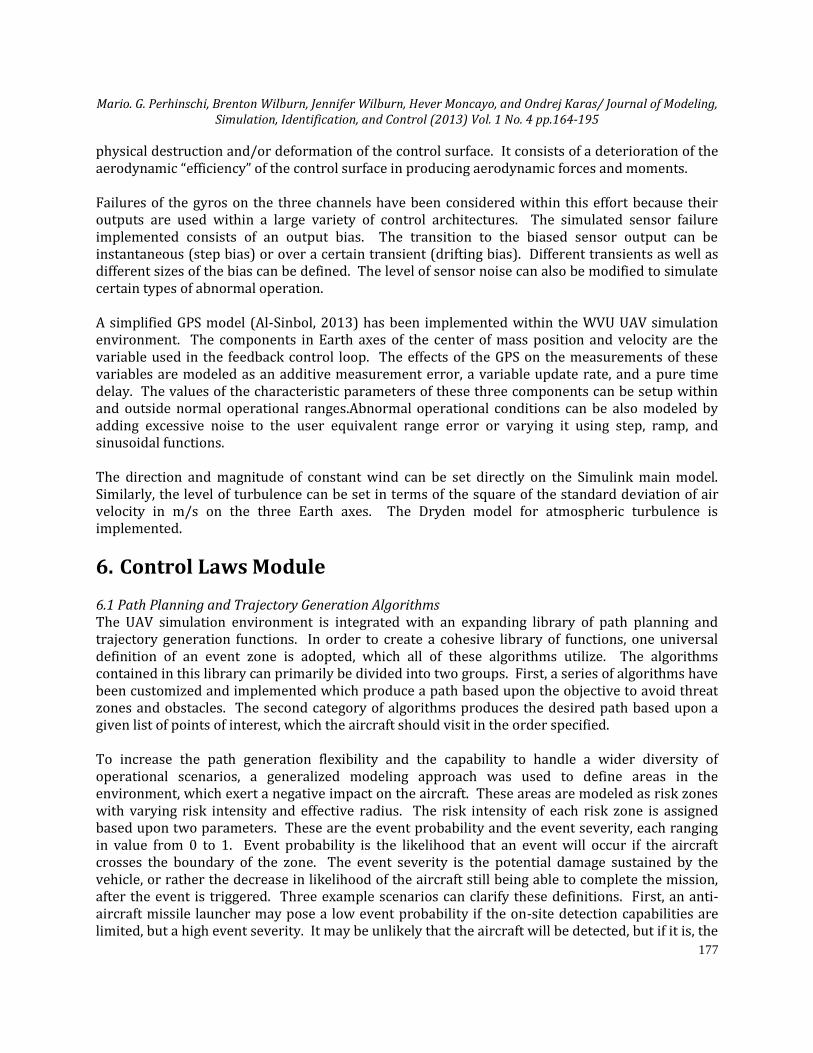
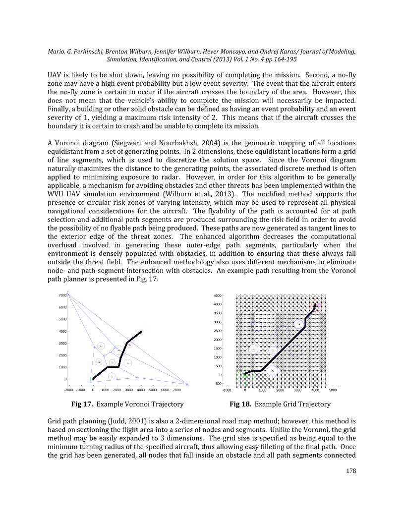
Fig 13. Pioneer Visual 3D Model Fig 14. Pioneer AVL Geometry. The all-composite TigerShark UAV operated by the U.S. Army is an example of a long-endurance aircraft (8-10 hours) with similar geometrical characteristics as Pioneer (see Fig. 15). It features a wingspan of 17’6” and a maximum take-off weight of 318lbs (Anon., 2009d). Given these similar characteristics, the aerodynamic model of the TigerShark within the WVU UAV simulation environment was obtained by altering the AVL stability and control derivatives with the Pioneer correction factors and terms, as described earlier. The moments of inertia were estimated based on a simplified geometric decomposition of aircraft components, assuming uniform weight distribution throughout the components, and estimating the weight of significant parts based on actual data and statistics. The OX UAV is a low-cost platform that offers great versatility allowing for various types of payload, which can be either carried internally, or on two under-wing hardpoints (Anon., 2011). The aircraft has a wingspan of 15’ and a maximum take-off weight of 110lbs. It features an inverted V-tail configuration with control surfaces that can in principle be used to control two different channels: pitch, using symmetrical deflections, or yaw, using differential deflections. Although the two tail control surfaces feature independent servos, the control software currently present on the aircraft only allows pitch control using the tail surfaces. However, a ruddervator control derivative was calculated for use in the WVU UAV simulation environment. The methodology based on AVL modeling augmented with correction factors and terms has been used for the development of the OX aerodynamic model. Fig. 16 presents the OX UAV geometrical model used with AVL. Based on limited flight data provided by the manufacturer and additional simulation experiments, a thrust lookup table with aircraft velocity as an input was produced (Karas, 2012). A simplified stall model was built from lift and drag curves for the NACA 63-415 airfoil, which is used for the wing of the OX UAV. The raw lift and drag data was subsequently adjusted for wing incidence and scaled to match the maximum lift coefficient at stall, as well as the drag coefficient at dash speed. All data points were finally entered into lookup tables for angle of attack contributions to lift and drag, effectively creating a stall model. Data was extrapolated for negative angles of attack down to -30 degrees as well. This model was then retrofitted to the Pioneer and TigerShark UAV models with adjustments for the specific airfoil characteristics of both Pioneer and TigerShark,


176

and the data was re-scaled to accommodate the most important data points: lift at maximum angle of attack and drag at dash speed (Karas, 2012).

Fig 15. TigerShark FlightGear Visualization Fig 16. OX UAV AVL Geometrical Model A simplified landing gear model was implemented within the WVU UAV simulation environment based on a more complex existing model (Evans et al., 2010). Spring, damper, and friction models are used to calculate the forces and moments produced by the landing gear on the vehicle. Note that landing gear simulation involves faster dynamics, which require a lower integration step than the general simulation. A crash model has also been implemented, which considers the position of five critical points on the aircraft with respect to the ground. These five points are: wing tips, H-tail tips, and nose. If any of these points becomes in contact with the ground, the simulation will stop. This also accounts for hard landings albeit in correct aircraft attitude, because an excessive compression of landing gear struts will cause the H-tail tips become in contact with the ground.

5. Abnormal Conditions Module Failures affecting the aerodynamic control surfaces (rudder, stabilator, and ailerons) and the sensors used in the control loop (gyros and GPS) have been modeled and implemented for the YF-22 UAV. These models are currently extended to other platforms. Note that the GTM has its specific implementation of actuator, sensor, structure, and engine failures. Two types of aerodynamic control surface failure are modeled: jammed surface and physically damaged surface (Perhinschi et al., 2008).The first failure type corresponds to an actuator mechanism failure and results in a locked surface; in fact, at the failure occurrence, the control surface moves to a pre-defined position and remains fixed there. A failure involving a blockage of the control surface at a fixed deflection does not alter the aerodynamic properties of the control surface. However, each surface in a pair (left and right) will have different deflections and the resulting moments and forces are computed individually. The second failure type corresponds to a


177

physical destruction and/or deformation of the control surface. It consists of a deterioration of the aerodynamic “efficiency” of the control surface in producing aerodynamic forces and moments. Failures of the gyros on the three channels have been considered within this effort because their outputs are used within a large variety of control architectures. The simulated sensor failure implemented consists of an output bias. The transition to the biased sensor output can be instantaneous (step bias) or over a certain transient (drifting bias). Different transients as well as different sizes of the bias can be defined. The level of sensor noise can also be modified to simulate certain types of abnormal operation. A simplified GPS model (Al-Sinbol, 2013) has been implemented within the WVU UAV simulation environment. The components in Earth axes of the center of mass position and velocity are the variable used in the feedback control loop. The effects of the GPS on the measurements of these variables are modeled as an additive measurement error, a variable update rate, and a pure time delay. The values of the characteristic parameters of these three components can be setup within and outside normal operational ranges.Abnormal operational conditions can be also modeled by adding excessive noise to the user equivalent range error or varying it using step, ramp, and sinusoidal functions. The direction and magnitude of constant wind can be set directly on the Simulink main model. Similarly, the level of turbulence can be set in terms of the square of the standard deviation of air velocity in m/s on the three Earth axes. The Dryden model for atmospheric turbulence is implemented.

6. Control Laws Module 6.1 Path Planning and Trajectory Generation Algorithms The UAV simulation environment is integrated with an expanding library of path planning and trajectory generation functions. In order to create a cohesive library of functions, one universal definition of an event zone is adopted, which all of these algorithms utilize. The algorithms contained in this library can primarily be divided into two groups. First, a series of algorithms have been customized and implemented which produce a path based upon the objective to avoid threat zones and obstacles. The second category of algorithms produces the desired path based upon a given list of points of interest, which the aircraft should visit in the order specified. To increase the path generation flexibility and the capability to handle a wider diversity of operational scenarios, a generalized modeling approach was used to define areas in the environment, which exert a negative impact on the aircraft. These areas are modeled as risk zones with varying risk intensity and effective radius. The risk intensity of each risk zone is assigned based upon two parameters. These are the event probability and the event severity, each ranging in value from 0 to 1. Event probability is the likelihood that an event will occur if the aircraft crosses the boundary of the zone. The event severity is the potential damage sustained by the vehicle, or rather the decrease in likelihood of the aircraft still being able to complete the mission, after the event is triggered. Three example scenarios can clarify these definitions. First, an anti-aircraft missile launcher may pose a low event probability if the on-site detection capabilities are limited, but a high event severity. It may be unlikely that the aircraft will be detected, but if it is, the


178

UAV is likely to be shot down, leaving no possibility of completing the mission. Second, a no-fly zone may have a high event probability but a low event severity. The event that the aircraft enters the no-fly zone is certain to occur if the aircraft crosses the boundary of the area. However, this does not mean that the vehicle’s ability to complete the mission will necessarily be impacted. Finally, a building or other solid obstacle can be defined as having an event probability and an event severity of 1, yielding a maximum risk intensity of 2. This means that if the aircraft crosses the boundary it is certain to crash and be unable to complete its mission. A Voronoi diagram (Siegwart and Nourbakhsh, 2004) is the geometric mapping of all locations equidistant from a set of generating points. In 2 dimensions, these equidistant locations form a grid of line segments, which is used to discretize the solution space. Since the Voronoi diagram naturally maximizes the distance to the generating points, the associated discrete method is often applied to minimizing exposure to radar. However, in order for this algorithm to be generally applicable, a mechanism for avoiding obstacles and other threats has been implemented within the WVU UAV simulation environment (Wilburn et al., 2013). The modified method supports the presence of circular risk zones of varying intensity, which may be used to represent all physical navigational considerations for the aircraft. The flyability of the path is accounted for at path selection and additional path segments are produced surrounding the risk field in order to avoid the possibility of no flyable path being produced. These paths are now generated as tangent lines to the exterior edge of the threat zones. The enhanced algorithm decreases the computational overhead involved in generating these outer-edge path segments, particularly when the environment is densely populated with obstacles, in addition to ensuring that these always fall outside the threat field. The enhanced methodology also uses different mechanisms to eliminate node- and path-segment-intersection with obstacles. An example path resulting from the Voronoi path planner is presented in Fig. 17.

Fig 17. Example Voronoi Trajectory Fig 18. Example Grid Trajectory Grid path planning (Judd, 2001) is also a 2-dimensional road map method; however, this method is based on sectioning the flight area into a series of nodes and segments. Unlike the Voronoi, the grid method may be easily expanded to 3 dimensions. The grid size is specified as being equal to the minimum turning radius of the specified aircraft, thus allowing easy filleting of the final path. Once the grid has been generated, all nodes that fall inside an obstacle and all path segments connected

-2000 -1000 0 1000 2000 3000 4000 5000 6000 7000

0

1000

2000

3000

4000

5000

6000

7000

-1000 0 1000 2000 3000 4000 5000

-500

0

500

1000

1500

2000

2500

3000

3500

4000

4500


179

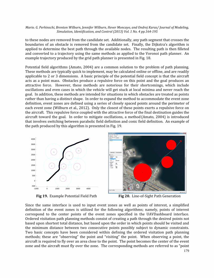
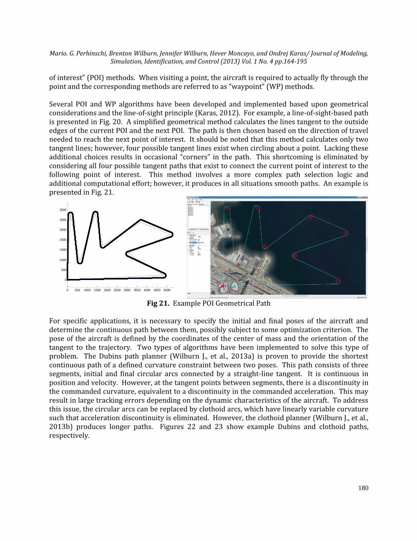
to these nodes are removed from the candidate set. Additionally, any path segment that crosses the boundaries of an obstacle is removed from the candidate set. Finally, the Dijkstra’s algorithm is applied to determine the best path through the available nodes. The resulting path is then filleted and converted to a trajectory using the same methods as applied to the Voronoi path planner. An example trajectory produced by the grid path planner is presented in Fig. 18. Potential field algorithms (Amato, 2004) are a common solution to the problem of path planning. These methods are typically quick to implement, may be calculated online or offline, and are readily applicable to 2 or 3 dimensions. A basic principle of the potential field concept is that the aircraft acts as a point mass. Obstacles produce a repulsive force on this point and the goal produces an attractive force. However, these methods are notorious for their shortcomings, which include oscillations and even cases in which the vehicle will get stuck at local minima and never reach the goal. In addition, these methods are intended for situations in which obstacles are treated as points rather than having a distinct shape. In order to expand the method to accommodate the event zone definition, event zones are defined using a series of closely spaced points around the perimeter of each event zone (Wilburn et al., 2012). Only the closest of these points exerts a repulsive force on the aircraft. This repulsive force coupled with the attractive force of the final destination guides the aircraft toward the goal. In order to mitigate oscillations, a method (Amato, 2004) is introduced that involves switching between parabolic field definition and conic field definition. An example of the path produced by this algorithm is presented in Fig. 19.

Fig 19. Example Potential Field Path Fig 20. Line-of-Sight Path Generation Since the same interface is used to input event zones as well as points of interest, a simplified definition of the event zones is utilized for the following algorithms; namely, points of interest correspond to the center points of the event zones specified in the UAVDashboard interface. Ordered visitation path planning methods consist of creating a path through the desired points not based upon shortest total distance, but based upon the order in which points should be visited and the minimum distance between two consecutive points possibly subject to dynamic constraints. Two basic concepts have been considered within defining the ordered visitation path planning methods; these are “observing” the point and “visiting” the point. When observing a point, the aircraft is required to fly over an area close to the point. The point becomes the center of the event zone and the aircraft must fly over the zone. The corresponding methods are referred to as “point

-1000 0 1000 2000 3000 4000

-500

0

500

1000

1500

2000

2500

3000

3500

4000


180

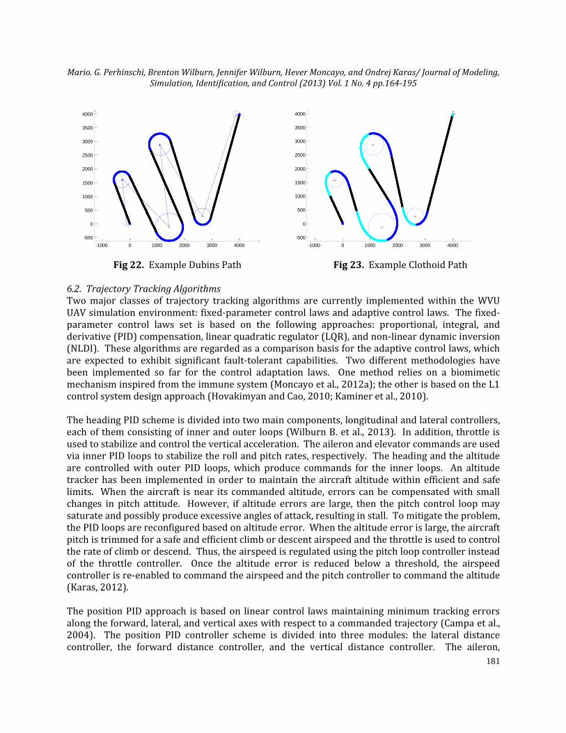
of interest” (POI) methods. When visiting a point, the aircraft is required to actually fly through the point and the corresponding methods are referred to as “waypoint” (WP) methods. Several POI and WP algorithms have been developed and implemented based upon geometrical considerations and the line-of-sight principle (Karas, 2012). For example, a line-of-sight-based path is presented in Fig. 20. A simplified geometrical method calculates the lines tangent to the outside edges of the current POI and the next POI. The path is then chosen based on the direction of travel needed to reach the next point of interest. It should be noted that this method calculates only two tangent lines; however, four possible tangent lines exist when circling about a point. Lacking these additional choices results in occasional “corners” in the path. This shortcoming is eliminated by considering all four possible tangent paths that exist to connect the current point of interest to the following point of interest. This method involves a more complex path selection logic and additional computational effort; however, it produces in all situations smooth paths. An example is presented in Fig. 21.

Fig 21. Example POI Geometrical Path

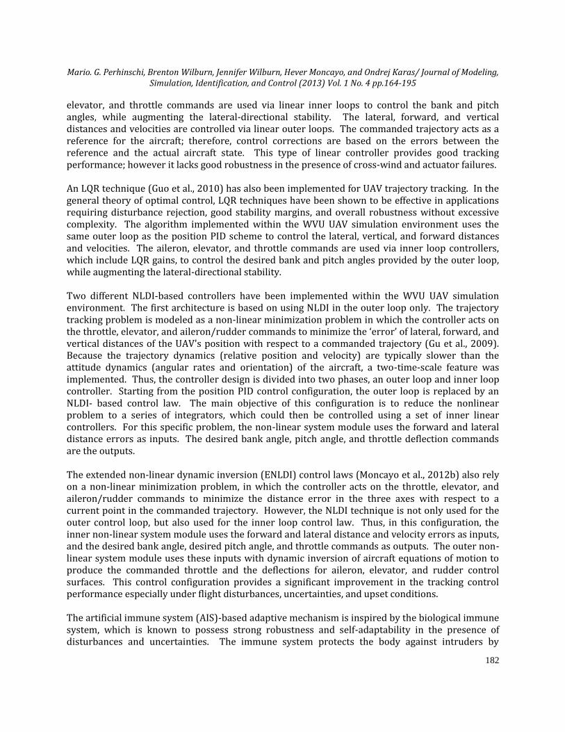
For specific applications, it is necessary to specify the initial and final poses of the aircraft and determine the continuous path between them, possibly subject to some optimization criterion. The pose of the aircraft is defined by the coordinates of the center of mass and the orientation of the tangent to the trajectory. Two types of algorithms have been implemented to solve this type of problem. The Dubins path planner (Wilburn J., et al., 2013a) is proven to provide the shortest continuous path of a defined curvature constraint between two poses. This path consists of three segments, initial and final circular arcs connected by a straight-line tangent. It is continuous in position and velocity. However, at the tangent points between segments, there is a discontinuity in the commanded curvature, equivalent to a discontinuity in the commanded acceleration. This may result in large tracking errors depending on the dynamic characteristics of the aircraft. To address this issue, the circular arcs can be replaced by clothoid arcs, which have linearly variable curvature such that acceleration discontinuity is eliminated. However, the clothoid planner (Wilburn J., et al., 2013b) produces longer paths. Figures 22 and 23 show example Dubins and clothoid paths, respectively.

0 500 1000 1500 2000 2500 3000 3500 4000 4500 5000

0

500

1000

1500

2000

2500

3000

3500


181

Fig 22. Example Dubins Path Fig 23. Example Clothoid Path 6.2. Trajectory Tracking Algorithms Two major classes of trajectory tracking algorithms are currently implemented within the WVU UAV simulation environment: fixed-parameter control laws and adaptive control laws. The fixed-parameter control laws set is based on the following approaches: proportional, integral, and derivative (PID) compensation, linear quadratic regulator (LQR), and non-linear dynamic inversion (NLDI). These algorithms are regarded as a comparison basis for the adaptive control laws, which are expected to exhibit significant fault-tolerant capabilities. Two different methodologies have been implemented so far for the control adaptation laws. One method relies on a biomimetic mechanism inspired from the immune system (Moncayo et al., 2012a); the other is based on the L1 control system design approach (Hovakimyan and Cao, 2010; Kaminer et al., 2010). The heading PID scheme is divided into two main components, longitudinal and lateral controllers, each of them consisting of inner and outer loops (Wilburn B. et al., 2013). In addition, throttle is used to stabilize and control the vertical acceleration. The aileron and elevator commands are used via inner PID loops to stabilize the roll and pitch rates, respectively. The heading and the altitude are controlled with outer PID loops, which produce commands for the inner loops. An altitude tracker has been implemented in order to maintain the aircraft altitude within efficient and safe limits. When the aircraft is near its commanded altitude, errors can be compensated with small changes in pitch attitude. However, if altitude errors are large, then the pitch control loop may saturate and possibly produce excessive angles of attack, resulting in stall. To mitigate the problem, the PID loops are reconfigured based on altitude error. When the altitude error is large, the aircraft pitch is trimmed for a safe and efficient climb or descent airspeed and the throttle is used to control the rate of climb or descend. Thus, the airspeed is regulated using the pitch loop controller instead of the throttle controller. Once the altitude error is reduced below a threshold, the airspeed controller is re-enabled to command the airspeed and the pitch controller to command the altitude (Karas, 2012). The position PID approach is based on linear control laws maintaining minimum tracking errors along the forward, lateral, and vertical axes with respect to a commanded trajectory (Campa et al., 2004). The position PID controller scheme is divided into three modules: the lateral distance controller, the forward distance controller, and the vertical distance controller. The aileron,

-1000 0 1000 2000 3000 4000

-500

0

500

1000

1500

2000

2500

3000

3500

4000

-1000 0 1000 2000 3000 4000

-500

0

500

1000

1500

2000

2500

3000

3500

4000


182

elevator, and throttle commands are used via linear inner loops to control the bank and pitch angles, while augmenting the lateral-directional stability. The lateral, forward, and vertical distances and velocities are controlled via linear outer loops. The commanded trajectory acts as a reference for the aircraft; therefore, control corrections are based on the errors between the reference and the actual aircraft state. This type of linear controller provides good tracking performance; however it lacks good robustness in the presence of cross-wind and actuator failures. An LQR technique (Guo et al., 2010) has also been implemented for UAV trajectory tracking. In the general theory of optimal control, LQR techniques have been shown to be effective in applications requiring disturbance rejection, good stability margins, and overall robustness without excessive complexity. The algorithm implemented within the WVU UAV simulation environment uses the same outer loop as the position PID scheme to control the lateral, vertical, and forward distances and velocities. The aileron, elevator, and throttle commands are used via inner loop controllers, which include LQR gains, to control the desired bank and pitch angles provided by the outer loop, while augmenting the lateral-directional stability. Two different NLDI-based controllers have been implemented within the WVU UAV simulation environment. The first architecture is based on using NLDI in the outer loop only. The trajectory tracking problem is modeled as a non-linear minimization problem in which the controller acts on the throttle, elevator, and aileron/rudder commands to minimize the ‘error’ of lateral, forward, and vertical distances of the UAV's position with respect to a commanded trajectory (Gu et al., 2009). Because the trajectory dynamics (relative position and velocity) are typically slower than the attitude dynamics (angular rates and orientation) of the aircraft, a two-time-scale feature was implemented. Thus, the controller design is divided into two phases, an outer loop and inner loop controller. Starting from the position PID control configuration, the outer loop is replaced by an NLDI- based control law. The main objective of this configuration is to reduce the nonlinear problem to a series of integrators, which could then be controlled using a set of inner linear controllers. For this specific problem, the non-linear system module uses the forward and lateral distance errors as inputs. The desired bank angle, pitch angle, and throttle deflection commands are the outputs. The extended non-linear dynamic inversion (ENLDI) control laws (Moncayo et al., 2012b) also rely on a non-linear minimization problem, in which the controller acts on the throttle, elevator, and aileron/rudder commands to minimize the distance error in the three axes with respect to a current point in the commanded trajectory. However, the NLDI technique is not only used for the outer control loop, but also used for the inner loop control law. Thus, in this configuration, the inner non-linear system module uses the forward and lateral distance and velocity errors as inputs, and the desired bank angle, desired pitch angle, and throttle commands as outputs. The outer non-linear system module uses these inputs with dynamic inversion of aircraft equations of motion to produce the commanded throttle and the deflections for aileron, elevator, and rudder control surfaces. This control configuration provides a significant improvement in the tracking control performance especially under flight disturbances, uncertainties, and upset conditions. The artificial immune system (AIS)-based adaptive mechanism is inspired by the biological immune system, which is known to possess strong robustness and self-adaptability in the presence of disturbances and uncertainties. The immune system protects the body against intruders by


183

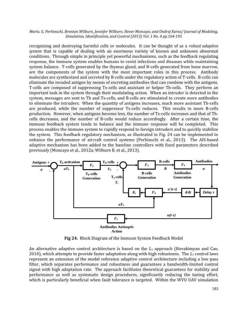
recognizing and destroying harmful cells or molecules. It can be thought of as a robust adaptive system that is capable of dealing with an enormous variety of known and unknown abnormal conditions. Through simple in principle yet powerful mechanisms, such as the feedback regulating response, the immune system enables humans to resist infections and diseases while maintaining system balance. T-cells generated by the thymus gland, and B-cells generated from bone marrow, are the components of the system with the most important roles in this process. Antibody molecules are synthesized and secreted by B-cells under the regulatory action of T-cells. B-cells can eliminate the invaded antigen by means of excreting antibodies that can combine with the antigens. T-cells are composed of suppressing Ts-cells and assistant or helper Th-cells. They perform an important task in the system through their modulating action. When an intruder is detected in the system, messages are sent to Th and Ts-cells, and B-cells are stimulated to create more antibodies to eliminate the intruders. When the quantity of antigens increases, much more assistant Th-cells are produced, while the number of suppressor Ts-cells reduces. This results in more B-cells production. However, when antigens become less, the number of Ts-cells increases and that of Th-cells decreases, and the number of B-cells would reduce accordingly. After a certain time, the immune feedback system tends to balance and the immune response will be completed. This process enables the immune system to rapidly respond to foreign intruders and to quickly stabilize the system. This feedback regulatory mechanism, as illustrated in Fig. 24 can be implemented to enhance the performance of aircraft control systems (Perhinschi et al., 2013). The AIS-based adaptive mechanism has been added to the baseline controllers with fixed parameters described previously (Moncayo et al., 2012a; Wilburn B. et al., 2013).

Fig 24. Block Diagram of the Immune System Feedback Model

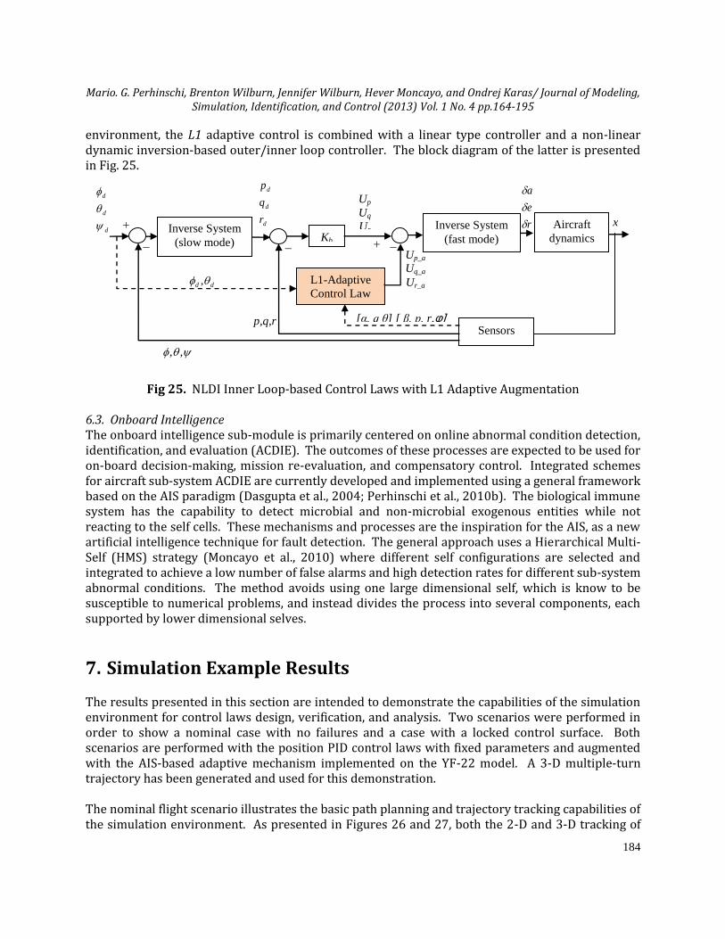
An alternative adaptive control architecture is based on the L1 approach (Hovakimyan and Cao, 2010), which attempts to provide faster adaptation along with high robustness. The L1 control laws represent an extension of the model reference adaptive control architecture including a low pass filter, which separates performance and robustness and guarantees a bandwidth-limited control signal with high adaptation rate. The approach facilitates theoretical guarantees for stability and performance as well as systematic design procedures, significantly reducing the tuning effort, which is particularly beneficial when fault tolerance is targeted. Within the WVU UAV simulation

+

-

F2 Antigens

a

Th activation

aTh

Th-cells +

-

Ts-cells

F3 F5

Th

Ts

B-cells

B

Th-cells

Generation

B-cells

Generation

Antibodies

Generation

Antibodies

u

Ks F4 Delay τ d/dt

u'(t-τ)

aTh

F1

u(t-τ)

Antibodies Antiseptic

Action


184

environment, the L1 adaptive control is combined with a linear type controller and a non-linear dynamic inversion-based outer/inner loop controller. The block diagram of the latter is presented in Fig. 25.

Up_a

Uq_a

Ur_a

[α, q θ] [ β, p, r,φ]

dd , L1-Adaptive

Control Law

r

e

a

,,

x

Inverse System

(fast mode)

Aircraft

dynamics Kb

p,q,r Sensors

d

d

d

r

q

p

Inverse System

(slow mode)

d

d

d

Up

Uq

Ur

Fig 25. NLDI Inner Loop-based Control Laws with L1 Adaptive Augmentation

6.3. Onboard Intelligence The onboard intelligence sub-module is primarily centered on online abnormal condition detection, identification, and evaluation (ACDIE). The outcomes of these processes are expected to be used for on-board decision-making, mission re-evaluation, and compensatory control. Integrated schemes for aircraft sub-system ACDIE are currently developed and implemented using a general framework based on the AIS paradigm (Dasgupta et al., 2004; Perhinschi et al., 2010b). The biological immune system has the capability to detect microbial and non-microbial exogenous entities while not reacting to the self cells. These mechanisms and processes are the inspiration for the AIS, as a new artificial intelligence technique for fault detection. The general approach uses a Hierarchical Multi-Self (HMS) strategy (Moncayo et al., 2010) where different self configurations are selected and integrated to achieve a low number of false alarms and high detection rates for different sub-system abnormal conditions. The method avoids using one large dimensional self, which is know to be susceptible to numerical problems, and instead divides the process into several components, each supported by lower dimensional selves.

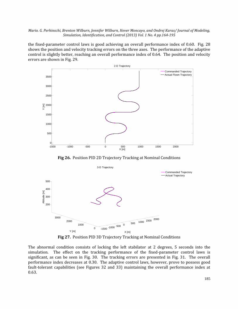
7. Simulation Example Results The results presented in this section are intended to demonstrate the capabilities of the simulation environment for control laws design, verification, and analysis. Two scenarios were performed in order to show a nominal case with no failures and a case with a locked control surface. Both scenarios are performed with the position PID control laws with fixed parameters and augmented with the AIS-based adaptive mechanism implemented on the YF-22 model. A 3-D multiple-turn trajectory has been generated and used for this demonstration. The nominal flight scenario illustrates the basic path planning and trajectory tracking capabilities of the simulation environment. As presented in Figures 26 and 27, both the 2-D and 3-D tracking of


185

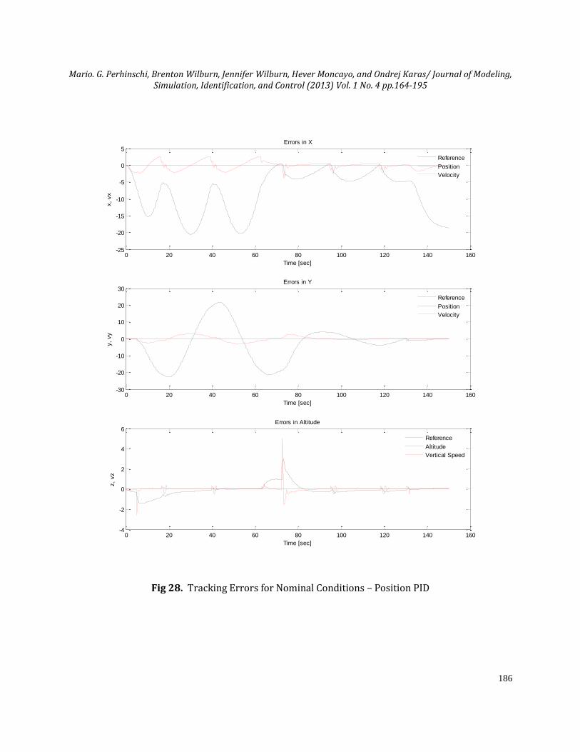
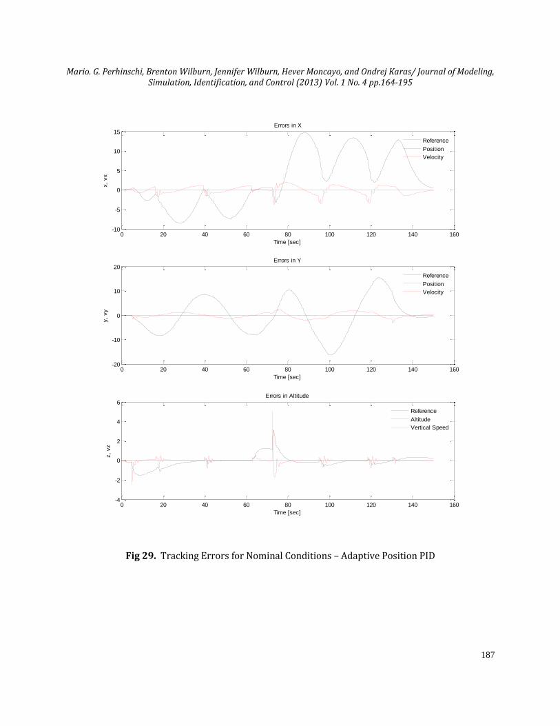
the fixed-parameter control laws is good achieving an overall performance index of 0.60. Fig. 28 shows the position and velocity tracking errors on the three axes. The performance of the adaptive control is slightly better, reaching an overall performance index of 0.64. The position and velocity errors are shown in Fig. 29.

Fig 26. Position PID 2D Trajectory Tracking at Nominal Conditions

Fig 27. Position PID 3D Trajectory Tracking at Nominal Conditions

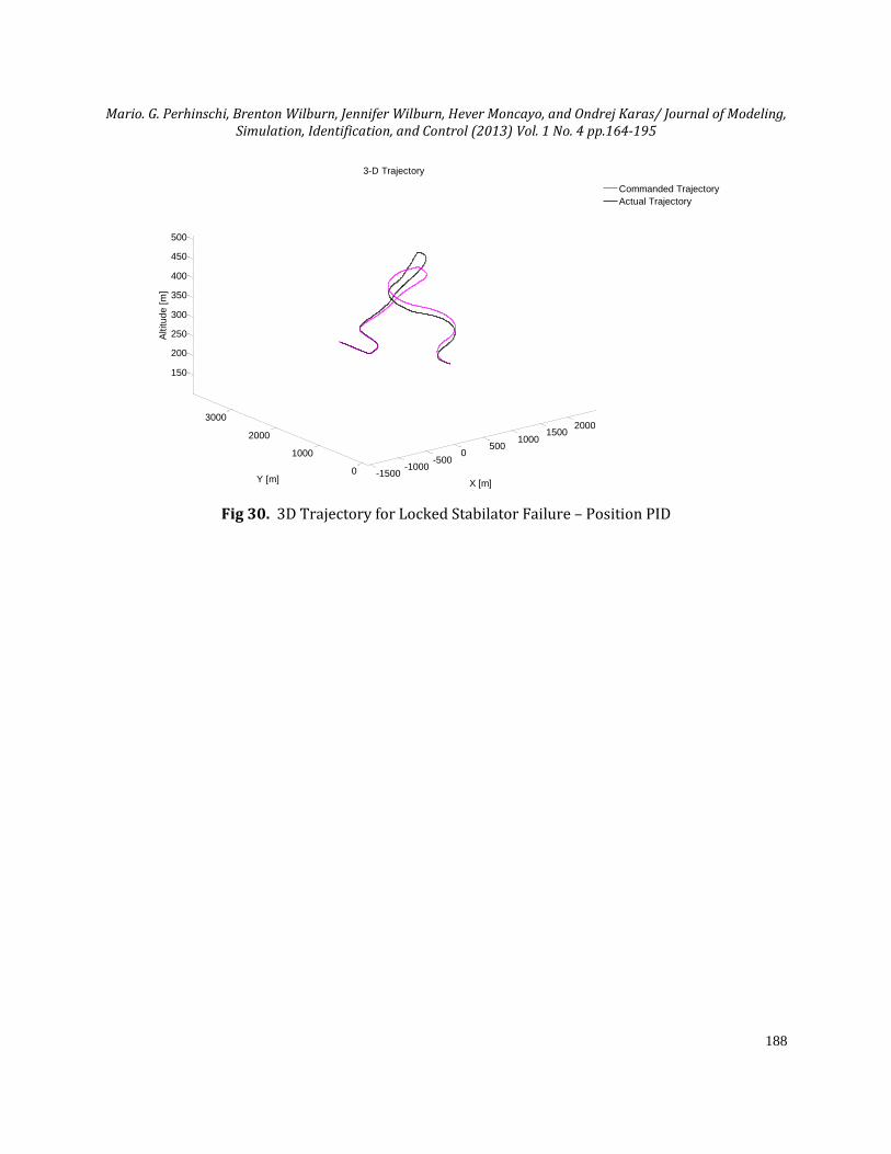
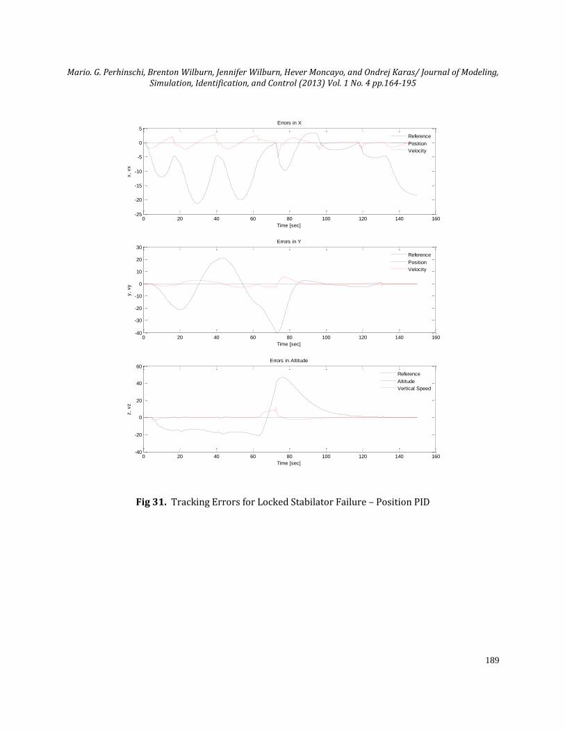
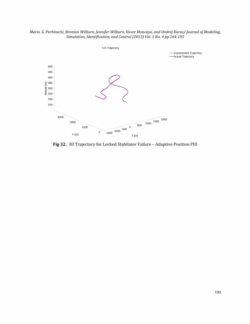
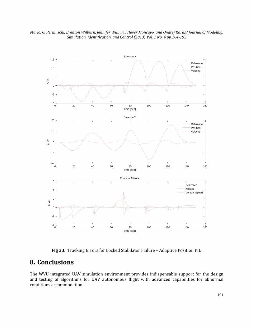
The abnormal condition consists of locking the left stabilator at 2 degrees, 5 seconds into the simulation. The effect on the tracking performance of the fixed-parameter control laws is significant, as can be seen in Fig. 30. The tracking errors are presented in Fig. 31. The overall performance index decreases at 0.30. The adaptive control laws, however, prove to possess good fault-tolerant capabilities (see Figures 32 and 33) maintaining the overall performance index at 0.63.

-1500 -1000 -500 0 500 1000 1500 2000

0

500

1000

1500

2000

2500

3000

3500

2-D Trajectory

X [m]

Y [

m]

Commanded Trajectory

Actual Flown Trajectory

-1500-1000

-5000

5001000

15002000

0

1000

2000

3000

200

300

400

500

X [m]

3-D Trajectory

Y [m]

Altitude [

m]


Actual Trajectory


186

Fig 28. Tracking Errors for Nominal Conditions – Position PID

0 20 40 60 80 100 120 140 160-25

-20

-15

-10

-5

0

5Errors in X

Time [sec]

x,

vx

Reference

Position

Velocity

0 20 40 60 80 100 120 140 160-30

-20

-10

0

10

20

30Errors in Y

Time [sec]

y,

vy

Reference

Position

Velocity

0 20 40 60 80 100 120 140 160-4

-2

0

2

4

6Errors in Altitude

Time [sec]

z,

vz

Reference

Altitude

Vertical Speed


187

Fig 29. Tracking Errors for Nominal Conditions – Adaptive Position PID

0 20 40 60 80 100 120 140 160-10

-5

0

5

10

15Errors in X

Time [sec]

x,

vx

Reference

Position

Velocity

0 20 40 60 80 100 120 140 160-20

-10

0

10

20Errors in Y

Time [sec]

y,

vy

Reference

Position

Velocity

0 20 40 60 80 100 120 140 160-4

-2

0

2

4

6Errors in Altitude

Time [sec]

z,

vz

Reference

Altitude

Vertical Speed


188

Fig 30. 3D Trajectory for Locked Stabilator Failure – Position PID

-1500-1000

-5000

5001000

15002000

0

1000

2000

3000

150

200

250

300

350

400

450

500

X [m]

3-D Trajectory

Y [m]

Altitude [

m]


Actual Trajectory


189

Fig 31. Tracking Errors for Locked Stabilator Failure – Position PID

0 20 40 60 80 100 120 140 160-25

-20

-15

-10

-5

0

5Errors in X

Time [sec]

x,

vx

Reference

Position

Velocity

0 20 40 60 80 100 120 140 160-40

-30

-20

-10

0

10

20

30Errors in Y

Time [sec]

y,

vy

Reference

Position

Velocity

0 20 40 60 80 100 120 140 160-40

-20

0

20

40

60Errors in Altitude

Time [sec]

z,

vz

Reference

Altitude

Vertical Speed


190

Fig 32. 3D Trajectory for Locked Stabilator Failure – Adaptive Position PID

-1500-1000

-5000

5001000

15002000

0

1000

2000

3000

150

200

250

300

350

400

450

500

X [m]

3-D Trajectory

Y [m]

Altitude [

m]


Actual Trajectory


191

Fig 33. Tracking Errors for Locked Stabilator Failure – Adaptive Position PID

8. Conclusions The WVU integrated UAV simulation environment provides indispensable support for the design and testing of algorithms for UAV autonomous flight with advanced capabilities for abnormal conditions accommodation.

0 20 40 60 80 100 120 140 160-10

-5

0

5

10

15Errors in X

Time [sec]

x,

vx

Reference

Position

Velocity

0 20 40 60 80 100 120 140 160-20

-10

0

10

20Errors in Y

Time [sec]

y,

vy

Reference

Position

Velocity

0 20 40 60 80 100 120 140 160-4

-2

0

2

4

6Errors in Altitude

Time [sec]

z,

vz

Reference

Altitude

Vertical Speed


192

The modular structure within Matlab/Simulink interfaced with FlightGear for visualization demonstrates maximum portability, flexibility, and extension capability. The UAV simulation environment provides the tools necessary to address several critical elements of autonomous flight algorithms including path planning, trajectory generation, trajectory tracking, situational awareness, decision-making, and overall intelligent operation.

Acknowledgements This work has been supported in part by U.S Army Research Laboratory under Cooperative Agreement no. W911NF-10-2-0110.

References Al-Sinbol, G., 2013.Analysis of GPS Abnormal Conditions within Fault Tolerant Control Laws.Master Thesis,

Department of Mechanical and Aerospace Engineering, West Virginia University, Morgantown, WV. Amato, N, 2004. Potential Field Methods. Randomized Motion Planning, University of Padova. Anon., 2009a. Unmanned Systems Integrated Roadmap 2009-2034. Office of the Secretary of Defense,

Washington, D.C. Anon., 2009b. UAV Simulator Solutions. H-SIM, Montesson, France. http://www.h-

sim.com/new_uav_sims.php (Accessed May 2013). Anon., 2009c. RQ-2A Pioneer Unmanned Aerial Vehicle (UAV). Public Affairs Office, Naval Air Station,

Patuxent River, Maryland. http://www.navy.mil/navydata/fact_display.asp?cid=1100&tid=2100&ct=1, (Accessed May 2013)

Anon. 2009d. TigerShark Data Sheet. Unmanned Aircraft System Solutions, L-3 Unmanned Systems, New York City, New York, http://www2.l-3com.com/uas/pdf_uas/tech/TigerShark.pdf, (Accessed May 2013).

Anon., 2010a. National Aeronautics Research and Development Policy. Executive Office of the President of the United States, National Science and Technology Council, http://www.whitehouse.gov/sites/default/files/microsites/ostp/aero-rdplan-2010.pdf (accessed May 2013).

Anon., 2010b. U.S. Army Unmanned Aircraft Systems Roadmap 2010-2035. U.S. Army UAS Center of Excellence, Fort Rucker, AL.

Anon., 2011. OX Unmanned Aerial Vehicle (UAV). CLMax Engineering LLC, Fort Walton Beach, Florida, http://clmaxengineering.com/ox01.html, (Accessed May 2012).

Anon., 2012a. FlightGear. http://www.flightgear.org (accessed May 2013). Anon., 2012b. X-Plane 10. http://www.x-plane.com (accessed May 2013). Bray, R., 1991. A Wind Tunnel Study of the Pioneer Remotely Piloted Vehicle, M.S. Thesis, Naval Postgraduate

School, Monterey, California. Campa, G., Napolitano, M.R., Seanor, B., Perhinschi, M.G., 2004. Design of Control Laws for Maneuvered

Formation Flight. Proc. of the 2004 American Control Conference, pp. 2344-2349, Boston, MA. Clark, I., Miksa, R., Childs, D., Mead, K., 1999. The Benefits of Simulation to Support Training. Armour Bulletin,

Vol. 32, No. 1. Craighead, J., Murphy, R., Burke, J., Goldiez, B., 2007. A Survey of Commercial & Open Source Unmanned

Vehicle Simulators. IEEE International Conference on Robotics and Automation, Rome, Italy. Dasgupta, D., KrishnaKumar, K., Wong, D., Berry, M., 2004. Negative Selection Algorithm for Aircraft Fault

Detection. G. Nicosia et al. (Eds.): ICARIS 2004, LNCS 3239, pp. 1–13.


193

De Crescenzio, F., Miranda, G., Persiani, F., Bombardi, T., 2007. Advanced interface for UAV (Unmanned Aerial Vehicle) Ground Control Station. Proc. of the AIAA Modeling and Simulation Technologies Conference and Exhibit, Hilton Head, South Carolina.

http://dx.doi.org/10.2514/6.2007-6566 Drela, M., Youngren H., 2007. AVL Overview, Massachusetts Institute of Technology, Cambridge,

Massachusetts, http://web.mit.edu/drela/Public/web/avl, accessed June 2013. Evans, P., Perhinschi, M.G., Mullins, S.,2010. Modeling and Simulation of a Tricycle Landing Gear at Normal

and Abnormal Conditions. Proc. of the AIAA Modeling and Simulation Technologies Conference, Toronto, Canada.

Freedy, A., Freedy, E., DeVisser, J., Weltman, G., Kalphat, M., Palmer, D., Coyeman, N., 2006. A Complete Simulation Environment for Measuring and Assessing Human-Robot Team Performance. IEEE Safety, Security, and Rescue Robotics Conference, Performance Metrics for Intelligent Systems Workshop, Gaithersburg, MD.

Gu, Y., Campa, G., Seanor, B., Gururajan, S., Napolitano, M.R., 2009. Aerial Autonomous Formation Flight – Design and Experiments. Aerial Vehicles. pp. 235-258, Edited by Thanh Mung Lam, Published by In-Tech, Kirchengasse 43/3, A-1070 Vienna, Austria.

Guo, J., Narkhede, S., Tao, G., 2010. An Adaptive LQ-Based Control Design with Parameter Projection Applied to the NASA GTM. Proc. of the AIAA Guidance, Navigation, and Control Conference, Toronto, Ontario, Canada.

http://dx.doi.org/10.2514/6.2010-7689 Hovakimyan, N. and Cao, C., 2010. L1 Adaptive Control Theory: Guaranteed Robustness with Fast Adaptation.

Society for Industrial and Applied Mathematics, Philadelphia, PA. http://dx.doi.org/10.1137/1.9780898719376 PMCid:PMC3065586 Jodeh, N., Blue, P., Waldron, A., 2006. Development of Small Unmanned Aerial Vehicle Research Platform:

Modeling and Simulating with Flight Test Validation. Proc. of the AIAA Modeling and Simulation Technologies Conference, Keystone, Colorado.

http://dx.doi.org/10.2514/6.2006-6261 Jordan, T. L., Langford, W. M., Hill, J. S., 2005. Airborne Subscale Transport Aircraft Research Testbed: Aircraft

Model Development. Proc. of the AIAA Guidance, Navigation, and Control Conference and Exhibit, San Francisco, CA.

http://dx.doi.org/10.2514/6.2005-6432 Jordan, T. L., Foster, J. V., Bailey, R. M. Belcastro, C. M., 2006. AirSTAR: A UAV Platform for Flight Dynamics and

Control System Testing. Proc. of the 25th AIAA Aerodynamic Measurement Technology and Ground Testing Conference, San Francisco, CA.

Judd, K., 2001. Trajectory Planning Strategies for Unmanned Aircraft. Brigham Young University Kaminer, I., Pascoal, A., Xargay, E., Hovakimyan, N., Cao, C., Dobrokhodov, V., 2010. Path Following for

Unmanned Aerial Vehicles Using L1 Adaptive Augmentation of Commercial Autopilots. Journal of Guidance, Control, and Dynamics, Vol. 33, No. 2, pp550-564.

http://dx.doi.org/10.2514/1.42056 Karas, O., 2012. UAV Simulation Environment for Autonomous Flight Control Algorithms. MS Thesis, West

Virginia University, Morgantown, WV. Kim, D., Kim, J., Kim, N., Suk, J., 2007. Development of Near-Real-Time Simulation Environment for Multiple

UAVs. EUROCON 2007 The International Conference on Computer as a Tool, Warsaw, Poland. Magrabi, S.M., Gibbens, P.W., 2000. Decentralized fault detection and diagnosis in navigation systems for

unmanned aerial vehicles. IEEE Symposium on Position Location and Navigation, San Diego, CA. Moncayo, H., Perhinschi, M.G., Davis, J., 2010. Artificial Immune System – Based Aircraft Failure Detection and

Identification Using an Integrated Hierarchical Multi-Self Strategy. AIAA Journal of Guidance, Control, and Dynamics, Vol. 33, No. 4, pp. 302-320.

http://dx.doi.org/10.2514/1.47445

http://dx.doi.org/10.2514/6.2007-6566

http://dx.doi.org/10.2514/6.2010-7689

http://dx.doi.org/10.1137/1.9780898719376

http://dx.doi.org/10.2514/6.2006-6261

http://dx.doi.org/10.2514/6.2005-6432

http://dx.doi.org/10.2514/1.42056

http://dx.doi.org/10.2514/1.47445


194

Moncayo, H., Perhinschi, M.G., Wilburn, B., Wilburn, J., Karas, O., 2012a. UAV Adaptive Control Laws Using Non-Linear Dynamic Inversion Augmented with an Immunity-based Mechanism. Proc. of the AIAA Guidance, Navigation, and Control Conference, Minneapolis, MN.

http://dx.doi.org/10.2514/6.2012-4678 Moncayo, H., Perhinschi, M.G., Wilburn, B., Wilburn, J., Karas, O., 2012b. Extended Nonlinear Dynamic

Inversion Control Laws for Unmanned Air Vehicles. Proc. of the AIAA Guidance, Navigation, and Control Conference, Minneapolis, MN.

http://dx.doi.org/10.2514/6.2012-4675 Mueller, E.R., 2007. Hardware-in-the-loop Simulation Design for Evaluation of Unmanned Aerial Vehicle

Control Systems. Proc. of the AIAA Modeling and Simulation Technologies Conference and Exhibit, Hilton Head, South Carolina.

http://dx.doi.org/10.2514/6.2007-6569 Napolitano, M.R., 2005. Development of Formation Flight Control Algorithms Using 3 YF-22 Flying Models.

AFSOR Final Report AFRL-SR-AR-TR-05-0164, Morgantown, West Virginia. Perhinschi, M.G., Napolitano, M.R., Campa, G., Seanor, B., Gururajan, S., 2004a. Design of Intelligent Flight

Control Laws for the WVU F-22 Model Aircraft. Proceedings of the AIAA Intelligent Systems Technical Conference, Chicago IL

http://dx.doi.org/10.2514/6.2004-6282 Perhinschi, M.G., Napolitano, M.R., Campa, G., Fravolini, M.L., 2004b. A Simulation Environment for Testing

And Research of Neurally Augmented Fault Tolerant Control Laws Based on Non-Linear Dynamic Inversion. Proceedings of the AIAA Modeling and Simulation Technologies Conference, Providence, Rhode Island.

http://dx.doi.org/10.2514/6.2004-4913 Perhinschi, M.G., Napolitano, M.R., Campa G., 2008. A Simulation Environment for Design and Testing of

Aircraft Adaptive Fault-Tolerant Control Systems. Aircraft Engineering and Aerospace Technology: An International Journal, Vol. 80, Iss. 6, pp 620-632.

Perhinschi, M.G., Napolitano, M.R., Tamayo S., 2010a. Integrated Simulation Environment For Unmanned Autonomous Systems – Towards A Conceptual Framework. Modelling and Simulation in Engineering, Vol. 2010, Article ID 736201, 12 pages, doi:10.1155/2010/736201.

http://dx.doi.org/10.1155/2010/736201 Perhinschi, M.G., Moncayo, H., Davis, J., 2010b. Integrated Framework for Artificial Immunity-Based Aircraft

Failure Detection, Identification, and Evaluation. AIAA Journal of Aircraft, Vol. 47, No. 6, pp. 1847-1859. http://dx.doi.org/10.2514/1.45718 Perhinschi, M.G., Moncayo, H., Davis, J., Wilburn, B., Karas, O., Wathen M., 2011. Development of a Simulation

Environment for Autonomous Flight Control Algorithms. Proceedings of the AIAA Guidance, Navigation, and Control Conference, Portland, Oregon.

Perhinschi, M.G., Moncayo, H., Al Azzawi, D., 2013. Development of Immunity-Based Framework for Aircraft Abnormal Conditions Detection, Identification, Evaluation, and Accommodation. Proc. of the AIAA Guidance, Navigation, and Control Conference, Boston, MA.

Rago, C., Prasanth, R., Mehra, R.K., Fortenbaugh R., 1998. Failure detection and identification and fault tolerant control using the IMM-KF with applications to the Eagle-Eye UAV. Proceedings of the 37th IEEE Conference on Decision and Control, Tampa, FL.

Rasmussen, S.J., Chandler, P.R., 2002. MultiUAV: A Multiple UAV Simulation for Investigation of Cooperative Control. Proc. of the 2002 Winter Simulation Conference, San Diego, CA.

Rauw, M. O., 1998. “FDC 1.2 – A SIMULINK Toolbox for Flight Dynamics and Control Analysis”, Delft University of Technology, Delft, The Netherlands.

Sardella, J.M., High, D.L., 2000. Integration of fielded army aviation simulators with ModSAF: The eighth army training solution. Proceedings of Interservice/Industry Training, Simulation and Education Conference, Orlando, FL.

http://dx.doi.org/10.2514/6.2012-4678

http://dx.doi.org/10.2514/6.2012-4675

http://dx.doi.org/10.2514/6.2007-6569

http://dx.doi.org/10.2514/6.2004-6282

http://dx.doi.org/10.2514/6.2004-4913

http://dx.doi.org/10.1155/2010/736201

http://dx.doi.org/10.2514/1.45718


195

Schaefer, P., Colgren, R.D., Abbott R.J., Park, H., Fijany, A., Fisher, F., James, M.L., Chien, S., Mackey, R., Zak, M., Johnson, T.L., Bush, S.F., 2000. Technologies for reliable autonomous control (TRAC) of UAVs. Proceedings of the 19th Digital Avionics Systems Conferences, Philadelphia, PA.

Siegwart, R. Nourbakhsh I. R., 2004. Planning and Navigation, Introduction to Autonomous Mobile Robots., pp. 257-272, MIT Press, Cambridge, Massachusetts.

Stevenson, D., Wheeler, M., Matlack, C., Wise, R., Whitacre, W.W., 2007. Developing a Robust and Flexible Simulation Environment to Support Cooperative Tracking of UAVs. Proc. of the AIAA Modeling and Simulation Technologies Conference and Exhibit, Hilton Head, South Carolina.

http://dx.doi.org/10.2514/6.2007-6565 Twesme, J., Corzine, A., 2003. Naval Air Systems Command (NAVAIR) Unmanned Aerial Vehicle (UAV)

Unmanned Combat Aerial Vehicle (UCAV) Distributed Simulation Infrastructure. 2nd AIAA "Unmanned Unlimited" Systems, Technologies, and Operations — Aerospace, Land, and Sea Conference and Workshop & Exhibit, San Diego, CA.

Wilburn, B., Perhinschi, M.G., Moncayo, H., Karas, O., Wilburn, J., 2013. Unmanned Aerial Vehicle Trajectory Tracking Algorithm Comparison. International Journal of Intelligent Unmanned Systems, accepted for publication, April 2013

Wilburn, J., Perhinschi, M.G., Wilburn, B., 2013. Enhanced Modified Voronoi Algorithm for UAV Path Planning and Obstacle Avoidance. International Review of Aerospace Engineering, Vol. 6, No. 1.

Wilburn, J., Cole, J., Perhinschi, M.G., Wilburn, B., 2012. Comparison of a Fuzzy Logic Controller to a Potential Field Controller for Real-Time UAV Navigation. Proc. of the AIAA Guidance, Navigation, and Control Conference, Minneapolis, MN.

http://dx.doi.org/10.2514/6.2012-4907 Wilburn, J., Perhinschi, M.G., Wilburn, B., 2013a. Implementation of a 3-Dimensional Dubins-Based UAV Path

Generation Algorithm. Proc. of the AIAA Guidance, Navigation, and Control Conference, Boston, MA. Wilburn, J., Perhinschi, M.G., Wilburn, B., 2013b. Implementation of Composite Clothoid Paths for Continuous

Curvature Trajectory Generation for UAVs. Proc. of the AIAA Guidance, Navigation, and Control Conference, Boston, MA.

Williams, K.W., 2006. Human Factors Implications of Unmanned Aircraft Accidents: Flight-Control Problems. Office of Aerospace Medicine, DOT/FAA/AM-06/8, Washington, DC.

http://dx.doi.org/10.2514/6.2007-6565

http://dx.doi.org/10.2514/6.2012-4907