![INDEX []€¦ · rule 704 regulated short selling 704.1 definition 704.2 permitted short selling 704.3 internal guidelines and systems 704.4 commencement of regulated short selling](https://static.fdocuments.in/doc/165x107/5eade3f34d23da570b2a62b0/index-rule-704-regulated-short-selling-7041-definition-7042-permitted-short.jpg)


Languages
Pages
Legal


Electronic copy available at: https://ssrn.com/abstract=2312625
1
Short Selling Risk
JOSEPH E. ENGELBERG, ADAM V. REED, and MATTHEW C. RINGGENBERG*
Forthcoming, Journal of Finance
ABSTRACT
Short sellers face unique risks, such as the risk that stock loans become expensive and the risk that
stock loans are recalled. We show that short selling risk affects prices among the cross-section of
stocks. Stocks with more short selling risk have lower returns, less price efficiency, and less short
selling.
JEL classification: G12, G14
Keywords: equity lending, limits to arbitrage, market efficiency, risk, short sale
* Joseph E. Engelberg, Rady School of Management, University of California, San Diego, [email protected].
Adam V. Reed, Kenan-Flagler Business School, University of North Carolina, [email protected]. Matthew C.
Ringgenberg, David Eccles School of Business, University of Utah, [email protected]. The
authors thank Ken Singleton (the editor), an anonymous associate editor, and two anonymous referees, as well as
Tom Boulton, Wes Chan, Itamar Drechsler, David Goldreich, Charles Jones, Juhani Linnainmaa, Paolo
Pasquariello, Burt Porter, David Sovich, Anna Scherbina; participants at the 2012 Data Explorers Securities
Financing Forum in New York, the 2013 IMN Beneficial Owner’s International Securities Lending Conference in
New Orleans, the 2013 RMA/UNC Securities Lending Institutional Contacts Academic and Regulatory Forum, the
6th Annual Florida State University SunTrust Beach Conference, the 2014 Financial Intermediation Research
Society conference, the 2014 LSE Conference on the Frontiers of Systemic Risk Modelling and Forecasting, the
2014 Western Finance Association annual meeting, the BlackRock WFA pre-conference, the 2014 BYU Red Rock
Finance Conference, the 2015 Wharton / Rodney L. White Center Conference on Financial Decisions and Asset
Markets; and seminar participants at Washington University in St. Louis, the University of Michigan, the University
of Cambridge, and the University of California - Irvine. We also thank Markit for providing equity lending data.
All errors are our own. Comments welcome. © 2012-2017 Joseph E. Engelberg, Adam V. Reed, and Matthew C.
Ringgenberg.

Electronic copy available at: https://ssrn.com/abstract=2312625
1
“Some stocks are hard to borrow. Herbalife is not, especially, but it is risky to
borrow…If Carl Icahn were to launch a tender offer, say, it might get a lot more expensive to
short Herbalife, and the convertible trade would become considerably less fun.”
Matt Levine, Former Investment Banker, BloombergView (2014)
Short selling is a risky business. Short sellers must identify mispriced securities, borrow shares
in the equity lending market, post collateral, and pay a loan fee each day until the position closes.
In addition to the standard risks that many traders face, such as a margin calls and regulatory
changes, short sellers also face the risk of loan recalls and the risk of changing loan fees. To
date, the existing literature has viewed these risks as a static cost to short sellers, and empirical
papers have shown that static impediments to short selling significantly affect asset prices and
efficiency.1 The idea in the literature is simple: if short selling is costly, short sellers may be less
likely to trade, and, as a result, prices may be biased or less efficient (e.g., Miller (1977),
Diamond and Verrecchia (1987), and Lamont and Thaler (2003)).
In this paper, we examine the costs of short selling from a different perspective.
Specifically, we show that the dynamic risks associated with short selling result in significant
1 To test the impact of impediments to short selling, existing studies have examined a wide variety of potential
measures of short sale constraints including regulatory action (Diether, Lee, and Werner (2009); Jones (2008);
Boehmer, Jones, and Zhang (2013); Battalio and Schultz (2011)); institutional ownership (Nagel (2005); Asquith,
Pathak, and Ritter (2005)); the availability of traded options (Figlewski and Webb (1993), Danielsen and Sorescu
(2001)); and current loan fees (Jones and Lamont (2002); Cohen, Diether, and Malloy (2009)). However, all of
these are static measures of short sale constraints (i.e., they examine how conditions today constrain short sellers),
while we focus on the dynamics of short selling constraints (i.e., we examine how the risk of changing future
constraints impacts short sellers).

Electronic copy available at: https://ssrn.com/abstract=2312625
2
limits to arbitrage. In particular, stocks with more short selling risk have lower future returns,
less price efficiency, and less short selling.
Consider two stocks – A and B – that are identical in every way except for their short
selling risk. Specifically, stock A and stock B have identical fundamentals and they have
identical loan fees and number of shares available today. However, future loan fees and share
availability are more uncertain for stock B than for stock A. In other words, there is considerable
risk that future loan fees for stock B will be higher and future shares of stock B will be
unavailable for borrowing. Since higher loan fees reduce the profits from short selling and
limited share availability can force short sellers to close their position before the arbitrage is
complete, a short seller would prefer to short stock A because it has lower short selling risk. In
this paper, we present the first evidence that uncertainty regarding future short sale constraints is
a significant risk, and we show that this risk affects trading and asset prices.
The short selling risk we describe has theoretical underpinnings in several existing
models. For example, in D’Avolio (2002b) and Duffie, Garleanu, and Pedersen (2002), short
selling fees and share availability are a function of the difference of opinions between optimists
and pessimists, and short selling risk emerges as these differences evolve. As noted by D’Avolio
(2002), “…a short seller is concerned not only with the level of fees, but also with fee variance.”
Accordingly, we focus on the variance of lending fees as our natural proxy for short selling risk.
To get the best possible measure of this proxy, we project the variance of lending fees on several
equity lending market characteristics and firm characteristics. We use fitted values from this
forecasting model (ShortRisk) as our measure of short selling risk.2
2 Our results are robust to using alternate measures of short selling risk, including the unconditional historical
variance of loan fees for each stock. These results are shown in the internet appendix.

3
Using this measure, we examine whether short selling risk affects arbitrage activity. If
short selling risk limits the ability of arbitrageurs to trade and correct mispricing, then it should
be related to returns, market efficiency, and short selling activity. We find that it is. First, we
show that our short selling risk proxy is related to future returns. A long-short portfolio formed
based on ShortRisk earns a 9.6% annual five-factor alpha. Moreover, in a Fama-MacBeth (1973)
regression framework we confirm the return predictability of short selling risk after controlling
for a variety of firm characteristics. In addition, we consider the Stambaugh, Yu, and Yuan
(2015) mispricing measure (MISP) and find that MISP’s ability to predict returns is greatest
among stocks with high short selling risk. Thus, higher short selling risk appears to limit the
ability of arbitrageurs to correct mispricing, and as a result, these stocks earn lower future
returns.3
Next, we test whether increases in short selling risk are associated with decreases in price
efficiency. We examine the Hou and Moskowitz (2005) measure of price delay and find that
short selling risk is associated with significantly larger price delay, even after controlling for
current loan market conditions (Saffi and Sigurdsson (2011)). A one standard deviation increase
in ShortRisk is associated with a 9.1% increase in price delay. In other words, the risk of future
short selling constraints is associated with decreased price efficiency today, independent of short
constraints that may exist at the time a short position is initiated.
3 This result is consistent with models of limits to arbitrage. For example, the model in Schleifer and Vishny (1997)
predicts that stocks that are riskier to arbitrage will exhibit greater mispricing and have higher average returns to
arbitrage.

4
Of course, if short selling risk is truly a limit to arbitrage, then we would expect this risk
to affect trading activity, especially for trades with a long expected time to completion.4 Ofek,
Richardson, and Whitelaw (2004) note that the, “…difficulty of shorting may increase with the
horizon length, as investors must pay the rebate rate spread over longer periods and short
positions are more likely to be recalled.” To test this prediction, we turn to one of the only cases
where mispricing and the expected holding horizon of a trade can be objectively measured ex-
ante. Specifically, we examine deviations between stock prices and the synthetic stock price
implied from put-call parity. Ofek, Richardson, and Whitelaw (2004) and Evans et al. (2009)
show that deviations between the actual and synthetic stock price often imply that a short seller
would short sell the underlying stock and purchase the synthetic stock, with the expectation that
the two prices will converge upon the option expiration date.
Accordingly, we measure mispricing using the natural log of the ratio of the actual stock
price to the implied stock price (henceforth put-call disparity) as in Ofek, Richardson, and
Whitelaw (2004), and we examine whether short sellers trade less on mispricings when short
selling risk is high and when the option has a long time to maturity. We find that they do. In
other words, arbitrageurs short significantly less when short selling risk is high, and, as a result,
there is more mispricing today. Moreover, both of these effects are significantly larger for long
horizon trades.
When ShortRisk and days to expiration are at the 25th percentile in our sample, short
volume is approximately 5.1% below its unconditional mean and put-call disparity today is
approximately 13.9% above its unconditional mean. However, when ShortRisk and days to
expiration are at the 75th percentile in our sample, short volume is 21.7% below its unconditional
4 We thank an anonymous referee and the editor for suggesting this point.

5
mean and put-call disparity today is approximately 149% above its unconditional mean.5 In
other words, higher short selling risk leads to significantly less short selling by arbitrageurs and
greater mispricing today, and longer holding horizons magnify both of these effects.
Of course, it is natural to expect that the risks we describe here could be correlated with
other well-known predictors of returns. For example, Ang et al. (2006) show that high
idiosyncratic volatility is associated with low future returns. We find that all of our results still
hold after controlling for other known predictors of returns, including liquidity and idiosyncratic
volatility (e.g., Ang et al. (2006), Pontiff (2006)).
Overall, our results make several contributions. First, and most importantly, we are the
first paper to show that uncertainty regarding future short selling constraints acts as a significant
limit to arbitrage; we show that higher short selling risk is associated with lower future returns,
decreased price efficiency, and less short selling activity by arbitrageurs. We also show that
these effects are magnified for trades with a long expected holding horizon. In addition, we
show that short selling risk is particularly high when there are extreme returns, indicating that
short selling risk may have an adverse correlation with returns. Finally, we note that our findings
may help explain existing anomalies, including the low short-interest puzzle (Lamont and Stein
(2004)). We also posit that short selling risk may explain the puzzling fact that short interest
data predict future returns even though short interest is publicly observable. In other words, the
fact that short interest data predict returns and is publicly released by the exchanges begs the
question: why don’t other investors arbitrage away the predictive ability of short interest? Our
results provide a partial explanation: short selling is risky.
5 The 25th and 75th percentiles of ShortRisk are 1.54 and 5.38, respectively. The 25th and 75th percentiles of months
to expiration are 2 and 5 months, respectively.

6
The remainder of this paper proceeds as follows: Section I briefly describes the existing
literature, Section II describes the data used in this study, Section III characterizes our findings,
and Section IV concludes.
I. Background
Although we consider short sale constraints from a dynamic perspective, a large literature
has considered these constraints from a static perspective. In this section, we briefly discuss
existing work concerning short sale constraints and limits to arbitrage. We then formalize the
hypotheses introduced in the beginning of the paper.
A. Existing Literature
On the theoretical side, multiple papers have argued that short sale constraints can have
an economically significant effect on asset prices (e.g., Miller (1977), Harrison and Kreps
(1978), Diamond and Verrecchia (1987)). In addition, empiricists have investigated multiple
forms of short selling constraints, including regulatory restrictions and equity loan fees.
Several papers have analyzed the effect of short sale constraints by examining changes in
the regulatory environment. For example, Diether, Lee, and Werner (2009) examine the effects
of the Reg SHO pilot and find that short selling activity increased when the uptick rule was
lifted. Boehmer, Jones, and Zhang (2013) find that the U.S. short selling ban reduced market
quality and liquidity. More broadly, Beber and Pagano (2013) find that worldwide short selling
restrictions slowed price discovery.
The equity loan market also provides an opportunity for researchers to study the impact
of short sale constraints. Using loan fees from the equity loan market, Geczy, Musto, and Reed

7
(2002) suggest that short selling constraints have a limited impact on well-accepted arbitrage
portfolios such as size, book-to-market, and momentum portfolios. Using institutional
ownership as a proxy for supply in the equity loan market, Hirshleifer, Teoh, and Yu (2011)
examine the relation between short sales and both the accrual and net operating asset anomalies.
They find that short sellers do try to arbitrage mispricings, but short sale constraints appear to
limit their ability to arbitrage them away.
Several papers abstract away from specific short sale constraints and instead use the
general fact that short selling is more constrained than buying to examine possible asymmetries
in long-short portfolio returns. Stambaugh, Yu, and Yuan (2012) examine a variety of anomalies
and find that they tend to be more pronounced on the short side, consistent with the idea that
short selling is riskier, thereby leading to less short selling by arbitrageurs. In a related paper,
Stambaugh, Yu, and Yuan (2015) note that idiosyncratic volatility is negatively related to returns
among underpriced stocks but is positively related to returns among overpriced stocks. More
recently, Drechsler and Drechsler (2014) document a shorting premium and show that asset
pricing anomalies are largest for stocks with high equity lending fees.
Finally, in a recent working paper, Prado, Saffi, and Sturgess (2014) examine the cross-
sectional relation between institutional ownership, short sale constraints, and abnormal stock
returns. They find that firms with lower levels of institutional ownership and/or more
concentrated institutional ownership tend to have higher equity lending fees, and these firms also
tend to earn abnormal returns that are significantly more negative.
B. Hypothesis Development

8
In this paper, we empirically examine the risk that future lending conditions might move
against a short seller. In what follows, we use existing theory to motivate our empirical
measures and develop testable predictions.
Several extant papers lend support for the idea that short selling risk will impact arbitrage
activity. Mitchell, Pulvino, and Stafford (2002) empirically examine arbitrage activity for
situations in which the market value of a company is less than its subsidiary and find that short
selling risk can limit arbitrage activity. They specifically discuss short selling risk, noting that,
“The possibility of being bought-in at an unattractive price provides a disincentive for
arbitrageurs to take a large position.” Consistent with this, D’Avolio (2002b) develops a
theoretical model of equilibrium in the lending market and finds that, “In a multiperiod setting, a
short seller is concerned not only with the level of fees, but also with fee variance. This is
because current regulations stipulate that lenders maintain the right to cancel a loan at any time
and hence preclude most large institutions from providing guaranteed term loans.”
In D’Avolio (2002b), a short seller can respond to changes in lending market conditions
by, “buying back the shares and returning them to the lender, or re-establishing the short at the
higher loan fee.” Thus, the model shows that share recalls and loan fee increases are two
manifestations of the same underlying event: changes in lending conditions that leave the loan
market temporarily out of equilibrium. As a result, recalls and fee changes are not independent
risks: a share recall can be seen as an extremely high loan fee. Consistent with theoretical
models, we develop two empirical measures of short selling risk in Section II, below. We view
our measures as proxies for the risk of short sale constraints that arise from changing lending
market conditions.

9
The model in D’Avolio (2002b) also suggests that lending market conditions will impact
arbitrage activity.6 Specifically, the model shows that short selling is less attractive to
arbitrageurs when short selling risk is high.7 While D’Avolio (2002b) does not explicitly model
the short seller’s demand function in the multiperiod case with short selling risk, a related model
in D’Avolio and Perold (2003) shows that short sellers will be less likely to trade if the
probability of binding future short sale constraints is high. Furthermore, this model also suggests
that the expected trading horizon will matter; D’Avolio and Perold (2003) show that short
sellers’ willingness to trade will be low when, “the expected price correction is unlikely to occur
in the near future.”
Accordingly, we use these results to generate several testable predictions regarding the
impact of short selling risk. First, we hypothesize that high short selling risk will be associated
with less trading by short sellers, consistent with the predictions in D’Avolio (2002 and 2002b)
and D’Avolio and Perold (2003). Second, consistent with models of limits to arbitrage (e.g.,
Schleifer and Vishny (1997)), we hypothesize that stocks with higher arbitrage risk, in this case
short selling risk, will exhibit greater mispricing. Third, as suggested by Ofek, Richardson, and
Whitelaw (2004) and D’Avolio and Perold (2003), we hypothesize that the impact of short
selling risk will be greater for trades with a longer expected holding horizon. Finally, we note
6 The model in Stambaugh, Yu, and Yuan (2015) can generate similar predictions. Specifically, if we introduce a
stochastic loan fee to the model, the solution to the utility maximization problem shows that portfolio weights are
decreasing in the variance of loan fees, and, as a consequence, mispricing is an increasing function of the variance of
loan fees. A theoretical derivation of this result is available from the authors upon request.
7 The model focuses primarily on a one-period case, in which equity lending conditions are known with certainty.
However, the paper includes a multiperiod extension that discusses short selling risk.

10
that the existing literature finds that short selling leads to improved price efficiency (Saffi and
Sigurdsson (2011)). This generates a fourth prediction: we hypothesize that stocks with more
short selling risk will have less price efficiency.
In sum, we hypothesize that arbitrageurs may be less willing to short when future lending
conditions are more uncertain and when the expected holding horizon is longer. As a result,
short selling risk may impact returns, price efficiency, and trading volume.
II. Data
To test the hypotheses discussed above, we combine daily equity lending data with data
from the Center for Research in Security Prices (CRSP), Compustat, the NYSE Trade and Quote
(TAQ) database, and OptionMetrics, as discussed in detail below.
A. Equity Lending Data
The equity lending data used in our analyses come from Markit. The data are sourced
from a variety of contributing customers including beneficial owners, hedge funds, investment
banks, lending agents, and prime brokers; the market participants that contribute to this database
are believed to account for the majority of all equity loans in the U.S. The initial database
includes information on a variety of overseas markets and share classes. However, we exclude
data on non-U.S. firms, ADRs, and ETFs, and we drop firms that have a stock price below $5 or
a market capitalization below $10 million; we also require each firm to have at least 50 non-
missing days each year to be included in the sample. The resulting database includes
approximately 220,000 observations at the firm-month level for 4,500 U.S. equities over the 5.5-
year period from July 1, 2006 through December 31, 2011.
11
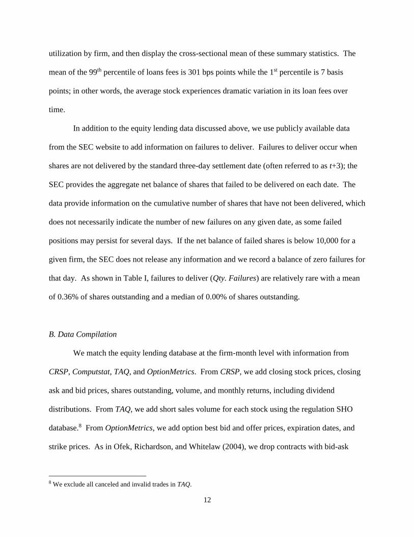
The equity lending database includes several variables from the equity loan market. Of
primary interest are shares borrowed (Short Interest), the active quantity of shares available to be
borrowed (Loan Supply), the active utilization rate (Utilization), the weighted average loan fee
across all shares currently on loan (Loan Fee), the weighted average loan fee for all new loans
over the past day (New Loan Fee), and the weighted average number of days that transactions
have been open (Loan Length). A stock’s Loan Supply represents the total number of shares that
institutions are actively willing to lend, expressed as a percentage of shares outstanding. The
Utilization is the quantity of shares loaned out as a percentage of Loan Supply. Finally, Loan
Fee, often referred to as specialness, is the cost of borrowing a share in basis points per annum.
INSERT TABLE I ABOUT HERE
Panel A of Table I contains summary statistics for the equity lending database. For the
typical firm, approximately 18% of outstanding shares are available to be borrowed and around
4% of shares outstanding are actually on loan at any given point. The median loan fee is only 11
basis points per annum; however, it is well known that loan fees exhibit considerable skewness,
as indicated by the mean of 85 basis points and the 99th percentile of 1,479 basis points. The
median loan is open for approximately 65 days, highlighting the fact that short sellers often hold
their position open for several months and thus are exposed to loan fee changes. Of course, the
magnitude of loan fees may seem small when compared to other risks faced by arbitrageurs,
especially when looking at the median loan fee of 11 bps. However, the 99th percentile of loan
fees in our sample is 14.79% per year; as discussed in Kolasinski, Reed, and Ringgenberg
(2013), loan fees can increase to levels that significantly decrease the profitability of nearly any
trade. Moreover, in Panel C we examine the within-firm (i.e., time-series) properties of lending
market conditions. We calculate the mean, median, 1st, and 99th percentiles of loan fees and
12
utilization by firm, and then display the cross-sectional mean of these summary statistics. The
mean of the 99th percentile of loans fees is 301 bps points while the 1st percentile is 7 basis
points; in other words, the average stock experiences dramatic variation in its loan fees over
time.
In addition to the equity lending data discussed above, we use publicly available data
from the SEC website to add information on failures to deliver. Failures to deliver occur when
shares are not delivered by the standard three-day settlement date (often referred to as t+3); the
SEC provides the aggregate net balance of shares that failed to be delivered on each date. The
data provide information on the cumulative number of shares that have not been delivered, which
does not necessarily indicate the number of new failures on any given date, as some failed
positions may persist for several days. If the net balance of failed shares is below 10,000 for a
given firm, the SEC does not release any information and we record a balance of zero failures for
that day. As shown in Table I, failures to deliver (Qty. Failures) are relatively rare with a mean
of 0.36% of shares outstanding and a median of 0.00% of shares outstanding.
B. Data Compilation
We match the equity lending database at the firm-month level with information from
CRSP, Computstat, TAQ, and OptionMetrics. From CRSP, we add closing stock prices, closing
ask and bid prices, shares outstanding, volume, and monthly returns, including dividend
distributions. From TAQ, we add short sales volume for each stock using the regulation SHO
database.8 From OptionMetrics, we add option best bid and offer prices, expiration dates, and
strike prices. As in Ofek, Richardson, and Whitelaw (2004), we drop contracts with bid-ask
8 We exclude all canceled and invalid trades in TAQ.

13
spreads greater than 50%, absolute value of log moneyness greater than 0.5, or non-positive
implied volatility. To minimize the impact of illiquidity, we focus on contracts with greater than
6 days but less than 181 days to maturity. From Compustat we add the natural log of the market-
to-book ratio. We define book equity as total shareholder equity minus the book value of
preferred stock plus the book value of deferred taxes and investment tax credit. If total
shareholder equity is missing, we calculate it as the sum of the book value of common and
preferred equity. If all of these are missing, we calculate shareholder equity as total assets minus
total liabilities. Finally, we add NYSE breakpoints and Fama and French (2015) factors from
Kenneth French’s website and we add the Stambaugh, Yu, and Yuan (2015) mispricing score
from Robert Stambaugh’s website. Panel B of Table I contains summary statistics for the CRSP
data. The mean market capitalization for the firms in our sample is $3.77 billion and the median
market capitalization is $0.46 billion.
C. Measures of Short Selling Risk
Motivated by the theoretical results discussed in Section I.B, we define a measure of short
selling risk (ShortRisk). The measure is motivated by D’Avolio (2002b), who notes that, “…a
short seller is concerned not only with the level of fees, but also with fee variance.” Consequently,
we calculate the natural log of the variance of the daily Loan Fee for each stock over the past 12
months and we project this variable on a variety of lagged firm and lending market characteristics.
The predicted values of the model, which we label ShortRisk, represents a trader’s estimate of
short selling risk given available information.
In our forecasting regression, we appeal to the prior literature in our choice of predictive
variables. Because Aggarwal, Saffi, and Sturgess (2015) demonstrate the importance of utilization

14
in the equity loan market, we consider prior loan utilization as a key forecasting variable.
Moreover, because Geczy, Musto, and Reed (2002) demonstrate the usefulness of prices from new
loans, we also consider the loan fees from new loans. Specifically, we use four equity lending
market characteristics: (i) VarNewFee, (ii) VarUtilization, (iii) TailNewFee, and (iv)
TailUtilization. VarNewFee is defined as the variance of loan fees for new equity loans and
VarUtilization is defined as the natural log of the variance of the ratio of equity loan supply to loan
demand (i.e., utilization). We also define two tail risk versions of these variables, TailFee and
TailUtilization, which proxy for the likelihood of extreme loan fees and extreme utilization,
respectively. Specifically, we define TailNewFee and TailUtilization as the 99th percentile of a
normal distribution using the trailing annual mean and variance of loan fee and utilization,
respectively.9
We also consider a number of potentially relevant firm characteristics, including a number
of characteristics that are worth noting in this context. Perhaps most important are lagged values
of fee risk, the number of fails to deliver, an indicator variable for stocks which had an IPO within
the last 90 days, and an indicator variable for stocks with listed options.
INSERT TABLE II ABOUT HERE
The results from the following model are presented in Table II:
𝑉𝑎𝑟(𝐿𝑜𝑎𝑛𝐹𝑒𝑒𝑠𝑖,𝑡+1) = α + 𝛽1𝑉𝑎𝑟𝑁𝑒𝑤𝐹𝑒𝑒𝑖,𝑡 + +𝛽2𝑉𝑎𝑟𝑈𝑡𝑖𝑙𝑖𝑧𝑎𝑡𝑖𝑜𝑛𝑖,𝑡 + 𝛽3𝑇𝑎𝑖𝑙𝑁𝑒𝑤𝐹𝑒𝑒𝑖,𝑡 + 𝛽4𝑇𝑎𝑖𝑙𝑈𝑡𝑖𝑙𝑖𝑧𝑎𝑡𝑖𝑜𝑛𝑖,𝑡 + FEi + FirmCharacteristics + 휀𝑖,𝑡+1,
(1)
9 Our measures are based on the well-known value-at-risk measure and are calculated on each date for each stock as
the mean of loan fee (utilization) + 2.33 × variance of loan fees (utilization), where the mean and variance are
measured over the prior 250 trading days.

15
where FEi indicates a firm fixed effect and FirmCharacteristics is a vector of time-varying firm
characteristics. We display t-statistics calculated using standard errors clustered by firm and date.
Although our main interest in this section is to find an accurate forecast of short selling risk, the
results here shed some light on the underlying determinants of short selling risk. For example, the
negative and statistically significant coefficient on the option indicator variable suggests that short
selling risk is lower for stocks with traded options. Similarly, the positive and statistically
significant coefficients on the dividend indicator and the number of fails to deliver suggest that
short selling risk is higher immediately following an IPO and for stocks with a large number of
failures in the securities lending market. Overall, the model can explain 97% of the variation in
one-month-ahead short selling risk.
Accordingly, we use the predicted value from this model as a forecast of short selling risk,
which we call ShortRisk.10 Summary statistics for ShortRisk are shown in Panel D of Table I. The
mean value of ShortRisk exceeds the median and the 99th percentile indicates that there is
substantial variation in short selling risk in our sample of firms.
III. Results
In this section, we examine whether short selling risk affects prices and trading by
arbitrageurs. Overall, our findings suggest that higher short selling risk is a significant limit to
arbitrage.
10 We thank an anonymous Associate Editor for suggesting this analysis.

16
A. Does Short Selling Risk Impact Arbitrageurs?
Short sellers face a number of risks. In equilibrium, arbitrageurs should be compensated
for the risks they take (e.g., Shleifer and Vishny (1997)). In this section, we begin by showing
that high short selling risk is associated with lower future returns. We then show that high short
selling risk is associated with decreased price efficiency and less short selling by arbitrageurs.
A.1. Short Selling Risk and Future Returns
To start, we form simple portfolios formed by conditioning on our risk measures.
Specifically, each month we form portfolios by sorting firms into quintiles using the previous
month’s short selling risk. These equal-weighted portfolios are then held for one calendar month
and the exercise is repeated.
Figure 1 shows a strong relation between short selling risk and future returns. In Panel A
we plot the mean returns to portfolios formed by conditioning on short selling risk. Stocks in the
low short selling risk quintile earn monthly returns of 0.58% per month while stocks in the high
short selling risk quintile earn monthly returns of -0.49% per month. Thus, a long-short portfolio
formed by buying stocks with low short risk and shorting stocks with high short risk earns 1.08%
per month. In Panel B, we plot the cumulative returns to a long-short strategy over our 2006 to
2011 sample period. The long-short portfolios consistently earn large returns. Overall, Figure 1
shows a close connection between short selling risk and future returns.
INSERT FIGURE 1 ABOUT HERE
Of course, a key concern is whether our results are a form of the well-established relation
between short selling and future returns. Several papers have shown that high short interest
predicts low future returns at the stock level (Figlewski (1981), Senchack and Starks (1993),

17
Boehmer, Jones, and Zhang (2008)) and Rapach, Ringgenberg, and Zhou (2016) show that short
interest is a strong predictor of returns at the market level.
To address this issue, we first sort on short interest and then sort on our short selling risk
measures. The mean returns to these portfolios are shown in Panels A and B of Table III and
five-factor alphas from these portfolios are shown in Panels A and B in Table IV. In Panel A of
Table III, we show the equal-weighted portfolio returns by quintiles formed on the previous
month’s ShortRisk. Conditioning on the level of short interest in each row, the last column
shows mean portfolio returns to a strategy that goes long firms with ShortRisk in the lowest
quintile and short firms with ShortRisk in the highest quintile. As shown in row 1 (All Firms),
the long-short portfolio (shown in the gray box) earns a mean monthly return of 1.08%, which is
statistically significant at the 1% level. In the remaining rows of Table III, Panel A, we show the
returns for each quintile of short interest. Interestingly, a strategy that buys stocks with low
ShortRisk and shorts stocks with high ShortRisk earns positive and statistically significant long-
short portfolio returns in each of the five short interest quintiles. The monthly long-short
portfolio returns (shown in the gray box) range from 0.63% to 1.19% (7.5% to 14.2%
annualized). We stress that while the first row does not condition on short interest, the remaining
rows do. The results are broadly similar to each other, indicating that the effect is not subsumed
by the previously studied relation between short interest and returns.
INSERT TABLE III ABOUT HERE
INSERT TABLE IV ABOUT HERE
Of course, it is possible that our portfolio sorts inadvertently sort on other common risk
factors. Accordingly, Table IV repeats the portfolio exercise with five-factor alphas (Fama and
French (2015)). In all three panels the results confirm the findings in Table III. A long-short

18
portfolio formed by conditioning on our short selling risk measure earns a five-factor alpha of
0.80% per month (shown in the gray box). We also find that the results generally remain
significant and economically large after conditioning on the level of short interest. In other
words, Table IV, as with Table III, is consistent with models of limits to arbitrage: we find that
the returns to short selling are largest when arbitrage is riskiest.
To better understand how the results hold up throughout the cross section, we also
examine sorts on firm size (market capitalization) to see if the relation between short selling risk
and returns is concentrated in Micro, Small, or Big firms. As in Fama and French (2008), we
define Micro firms as firms with market capitalization below the 20th percentile of the NYSE
breakpoints from Kenneth French’s website, Small firms as firms with market capitalization
greater than or equal to the 20th percentile but less than the 50th percentile of NYSE breakpoints,
and Large firms as firms with market capitalization greater than or equal to the 50th percentile.
Within each size category, we sort into five buckets based on short selling risk. We then create
value-weighted portfolios and look at the next month’s return.11
Raw returns from this exercise are shown in Panel B of Table III, while Panel B in Table
IV shows Fama and French (2015) five-factor alphas. The results are generally strongest in
Micro and Small stocks; however, in Table III Large stocks do earn a positive long-short
portfolio return (but for these stocks the results exhibit weaker statistical significance). In Table
III we find positive and statistically significant long-short returns for both Micro and Small
stocks, ranging from 0.65% to 1.04%. Similarly, in Table IV we find positive and statistically
11 Because we require firms to have equity lending data, our sample contains fewer Micro stocks than the sample in
Fama and French (2008). Specifically, 60% of all stocks in the Fama and French (2008) sample are Micro stocks
but only 44% of the stocks in our sample are classified as Micro.

19
significant five-factor alphas for Micro and Small stocks, ranging from 0.38% to 0.88%. In a
sense, the fact that our results are strongest among Micro and Small stocks is not surprising as
there is relatively little short selling risk in the sample of Large stocks. The 99th percentile of
loan fees in the Micro sample is 1,119 bps; however, the 99th percentile of loan fees in the Large
stock sample is only 236 bps. Similarly, the 90th percentile is 189 bps for Micro stocks and only
20 bps for the Large stocks. In addition, we note that while Micro and Small stocks represent a
relatively small portion of total market capitalization, they are a large portion of the market, by
number. In our analyses, these stocks represent approximately 75% of the sample. Thus, while
our results are weaker among Large stocks, they do occur throughout a large portion of U.S.
equities.
Interestingly, we also note that our sort results suggest that low short selling risk stocks
are also priced differently. While the high short selling risk portfolios consistently earn negative
returns, many of the low short selling risk portfolios earn high returns, a result consistent with
Boehmer, Huszar, and Jordan (2010). Nonetheless, taken together, our sort results indicate that
arbitrageurs are being compensated for the risk they take on their short positions.12
12 In untabulated results, we repeat the sorts from Panels A and B of Tables III and IV, only we first sort on current
loan fees instead of short interest. We find that short risk generally matters the most when loan fees are high.
However, the results confirm that short selling risk matters even after controlling for the relation between the level
of loan fees and future returns.

20
Finally, we adopt the regression approach of Boehmer, Jones, and Zhang (2008) to
control for more firm characteristics.13 In particular, we run monthly Fama-MacBeth (1973)
regressions of the form:
𝑅𝑒𝑡𝑖,𝑡+1 = α + 𝛽1𝑆ℎ𝑜𝑟𝑡 𝑅𝑖𝑠𝑘𝑖,𝑡 + 𝛽2𝑆ℎ𝑜𝑟𝑡 𝐼𝑛𝑡𝑒𝑟𝑒𝑠𝑡𝑖,𝑡+ Controls + 휀𝑖,𝑡+1 (2)
where the dependent variable is the buy and hold return percent over the subsequent month,
excess of the one-month risk-free rate; Short Interesti,t is the quantity of shares borrowed as of
the last day of the month for each firm, normalized by each firm’s shares outstanding; and
Controls represents several different control variables. Market / Book is the log of the market-to-
book ratio from Compustat, Market Cap is the log of market capitalization, Idio. Volatility is the
log of the monthly standard deviation of the daily residual from a Fama-French three-factor
regression,14 Bid-Ask is the log of the closing bid-ask spread calculated as a fraction of the
closing mid-point, and Returnt-1 is the return on each stock lagged by one month.
INSERT TABLE V ABOUT HERE
Our contribution is to introduce a measure of an arbitrageur’s short selling risk. The
results are shown in Table V. In all models, the coefficient on Short Interest is consistent with
Boehmer, Jones, and Zhang (2008); we find that short sales activity, as measured by Short
13 While we follow a similar approach to that in Boehmer, Jones, and Zhang (2008), our specification includes
several differences. First, we use a different sample period then Boehmer, Jones, and Zhang (2008) and we examine
a different set of firms (we examine the entire CRSP universe of equities while they focus on NYSE firms).
Moreover, we use a measure of Short Interest as an independent variable, while they use Short Volume.
14 We calculate idiosyncratic volatility as the standard deviation, each month, of the daily residual from a Fama and
French (1993) three-factor model estimated using daily return data over our entire sample period.

21
Interest, is negative. In other words, high levels of short selling are associated with future price
decreases.
In all models the negative and statistically significant coefficient on ShortRisk is
consistent with the hypothesis that short selling risk is a significant limit to arbitrage.15 In
particular, we find in model (1) that a one standard deviation increase in ShortRisk is associated
with a 53 basis point decrease in future monthly returns (a decrease of approximately 6.3% per
year). In other words, on average, the returns to short selling are larger in the presence of greater
short selling risk.
In model (3), we consider how short selling risk, as a limit to arbitrage, interacts with
mispricing as measured by Stambaugh, Yu, and Yuan (2015). We refer to the mispricing
variable as MISP, and it is based on 11 anomalies from the existing literature.16 High (low)
values of the MISP variable are the most overpriced (underpriced) according to Stambaugh, Yu,
and Yuan (2015). When we interact ShortRisk and MISP, we find a negative and statistically
significant coefficient, which suggests that stocks that are both overpriced and risky to short have
especially low returns going forward.17 In other words, consistent with models of limits to
arbitrage, we find that higher short selling risk appears to limit the ability of arbitrageurs to
15 Because ShortRisk is a generated regressor (Pagan (1984)), we calculate the standard errors of the coefficients
using a block bootstrap with 200 replications. The bootstrap does not significantly alter the standard errors. The
results are qualitatively unchanged if we instead use Newey-West (1987) standard errors with 3 lags, where we set
the lag length = T¼ = 66¼ ≈ 3 as discussed in Greene (2002).
16 Stambaugh, Yu, and Yuan (2015) do not use any short selling-based anomalies in their mispricing measure.
17 In untabulated results, the coefficient estimate on MISP, when there is no interaction term, is negative and
significant as in Stambaugh, Yu, and Yuan (2015).

22
correct mispricing, and, as a result, these stocks earn lower future returns. As ShortRisk and
MISP increase, we find that future returns get lower. When both ShortRisk and MISP are at their
90th percentiles, the next month’s return is 22 basis points lower than when both ShortRisk and
MISP are at their 50th percentiles.
Overall, the findings in Tables III through V suggest that higher short selling risk limits
the ability of arbitrageurs to correct mispricing; as a result, stocks with high short selling risk
earn predictably lower future returns. Moreover, we note that we control for the current loan fee
in models (2) and (3) of Table V, since it is well known that high equity loan fees predict low
future stock returns (e.g., Jones and Lamont (2002), Beneish, Lee, and Nichols (2015), Drechsler
and Drechsler (2014)). Thus, our results show that the risk of future short selling constraints
affects returns even after controlling for current short sale constraints and other known predictors
of returns.
This evidence also sheds light on an unresolved puzzle. Several papers have shown that
high short interest predicts low future returns (Figlewski (1981), Senchack and Starks (1993),
Asquith, Pathak, and Ritter (2005), Boehmer, Jones, and Zhang (2008), Rapach, Ringgenberg,
and Zhou, (2016)), and thus it is puzzling that publicly available short interest data continue to
have return predictability. Our results show that this puzzle is particularly strong among stocks
with high short selling risk. Although the existing literature has been unable to fully explain the
puzzle with static short selling constraints (e.g., Cohen, Diether, and Malloy (2009)), our paper
suggests that dynamic constraints (i.e., short selling risk) may help explain more of the puzzle.
In other words, short sellers continue to earn abnormal returns, in part because short selling is
risky.

23
A.2. Short Selling Risk and Price Efficiency
Of course, if short selling risk is a limit to arbitrage it may also decrease price efficiency.
In this section, we use our proxies for short selling risk to test whether more short selling risk is
associated with less price efficiency. We first estimate the Hou and Moskowitz (2005) measures
of price efficiency by regressing the weekly returns of stock i on the current value-weighted
market return and four lags of the value-weighted market return. Intuitively, the coefficients on
lagged market returns are a measure of price delay; if the return on stock i instantaneously
reflects all available information, then the lagged returns should have little explanatory power.
Specifically, for each stock i and year y, we estimate the following regression:
𝑟𝑒𝑡𝑖,𝑡 = α + 𝛽1𝑖,𝑦
𝑟𝑚,𝑡 + (∑ 𝛿𝑗𝑖,𝑦
𝑟𝑚,𝑡−𝑗4𝑗=1 )+ 휀𝑖,𝑡 (3)
where reti,t is the return on stock i in week t and retm,t is the value-weighted market return from
CRSP in week t. We then calculate two measures of price delay, labeled D1 and D2, as follows:
𝐷1𝑖,𝑦 = 1 −𝑅[𝛿1=𝛿2=𝛿3=𝛿4=0]
2
𝑅2
(4)
where the denominator is the unconstrained R2 and the numerator is the R2 from a regression
where the coefficients on all lagged market returns are constrained to equal zero, and
𝐷2𝑖,𝑦 =∑ |𝛿𝑗
𝑖,𝑦|4
𝑗=1
|𝛽1𝑖,𝑦
| + ∑ |𝛿𝑗𝑖,𝑦
|4𝑗=1
(5)
where β and δ are the regression coefficients shown in equation (3). We then test to see if our
proxies for short selling risk are associated with increased price delay (i.e., worse price
efficiency). To do this, we estimate the following panel regression, similar to Saffi and
Sigurdsson (2011):

24
𝑃𝑟𝑖𝑐𝑒𝐷𝑒𝑙𝑎𝑦𝑖,𝑦= α + 𝛽1𝑆ℎ𝑜𝑟𝑡𝑅𝑖𝑠𝑘 + 𝛽2𝐿𝑜𝑎𝑛𝐹𝑒𝑒 + 𝛽3𝐿𝑜𝑎𝑛𝑆𝑢𝑝𝑝𝑙𝑦 + 𝐶𝑜𝑛𝑟𝑜𝑙𝑠 + 휀𝑖,𝑦 (6)
The results are shown in Table VI with t-statistics, calculated using a block bootstrap with 200
replications, shown below the coefficient estimates. We include year fixed effects in all models
to control for possible unobserved heterogeneity. Saffi and Sigurdsson (2011) examine the
relation between price efficiency and contemporaneous short sale constraints and they find that
firms with high loan supply tend to have significantly better price efficiency. The statistically
significant negative coefficient on Loan Supply confirms the findings of Saffi and Sigurdsson
(2011). However, we also find that uncertainty regarding future short sale constraints is
associated with decreased price efficiency. In all models, the positive and statistically significant
coefficient on ShortRisk indicates that higher uncertainty about future loan fees is associated
with a significantly larger price delay for the measure calculated in equation (4). In model (2), a
one standard deviation increase in ShortRisk is associated with a 9.1% increase in price delay
relative to its unconditional mean.18 In other words, the risk of future short selling constraints is
associated with decreased price efficiency today, independent of short constraints that may exist
at the time a short position is initiated.
INSERT TABLE VI ABOUT HERE
Taking the results in Table VI together, a general pattern emerges: higher short selling
risk is associated with decreased price efficiency.
A.3. Short Selling Risk and Expected Holding Horizon
18 ShortRisk has a standard deviation of 4.04 and the Hou and Moskowitz price delay measure has an unconditional
mean of 0.32; therefore, 9.1% = (0.0072 * 4.04) / 0.32.

25
If short selling risk is truly a limit to arbitrage, then we would expect this risk to affect
trading activity (D’Avolio (2002)), especially for trades with a long expected time to completion.
As Ofek, Richardson, and Whitelaw (2004) note, the risk of short selling will increase with the
holding period. For example, an arbitrageur shorting a stock with a volatile rebate rate is much
more concerned about the volatility if his expected holding horizon is long. As a result, the
arbitrageur is less likely to put on the trade in the first place.
To test this prediction, we examine a unique environment in which both the magnitude of
the mispricing and the expected holding horizon of a trade can be measured ex-ante.
Specifically, we examine a measure of mispricing from Ofek, Richardson, and Whitelaw (2004),
put-call disparity, which is defined as the log difference between the stock price from the spot
market and the synthetic stock price implied from put-call parity in the options market. Ofek,
Richardson, and Whitelaw (2004) and Evans et al. (2009) show that when put-call disparity is
positive, a short seller would want to short sell the underlying stock and purchase the synthetic
stock, and they would expect the two to converge by the option expiration date.
INSERT TABLE VII ABOUT HERE
Accordingly, Table VII examines the relation between put-call disparity, short selling
risk, and holding horizon using OLS panel regressions of the form:
𝑃𝑢𝑡𝐶𝑎𝑙𝑙𝐷𝑖𝑠𝑝𝑎𝑟𝑖𝑡𝑦𝑖,𝑡= 𝛽1𝑀𝑜𝑛𝑡ℎ𝑠 𝑡𝑜 𝐸𝑥𝑝𝑖,𝑡 + 𝛽2𝑆ℎ𝑜𝑟𝑡 𝑅𝑖𝑠𝑘𝑖,𝑡−1+ 𝛽3(𝑆ℎ𝑜𝑟𝑡 𝑅𝑖𝑠𝑘𝑖,𝑡−1×
𝑀𝑜𝑛𝑡ℎ𝑠 𝑡𝑜 𝐸𝑥𝑝𝑖,𝑡) + Controls + 𝐹𝐸𝑖 + 𝐹𝐸𝑡 + 휀𝑖,𝑡, (7)
where Months to Exp is our measure of the expected holding horizon of the arbitrageur and
defined as the number of months between an option’s expiration date and the current date.
ShortRisk is calculated as before but is now matched to the option expiration date. Specifically,
we run predictive regressions as in equation (1), where the dependent variable is loan fee

26
variance measured over 1 - 30 days, 31- 60 days, 61 - 90 days, and so on. Then we take this
forecast, ShortRisk, and use it as a predictor of PutCallDisparity measured using the same option
expiration window. This lets us match the holding horizon of the arbitrageur with the expected
short selling risk she will face over that horizon.
We include firm and date fixed effects in all models to control for possible unobserved
heterogeneity. The coefficient estimates are shown in Table VII with t-statistics (shown in
parentheses below the coefficient estimates) calculated using a block bootstrap with 200
replications. To examine the general relation between short selling risk and mispricing, in model
(1) we omit the interaction between ShortRisk and Months to Exp. In this specification, the
positive and statistically significant coefficient on short risk suggests that the no-arbitrage put-
call parity equation is more likely to be violated when short selling risk is high. In other words,
the results provide additional support for our main hypothesis: short selling risk leads to more
mispricing.
In models (2) and (3) we add an interaction term between ShortRisk and Months to Exp to
test whether short selling risk matters more for trades with a longer expected holding period. We
find evidence that it does. In model (3), the statistically significant coefficient of 0.0303 on the
interaction term suggests that put-call disparity is 13.9% above its unconditional mean when
both ShortRisk and Months to Expiration are at the 25th percentile in our sample, but the effect
increases to 149% when both ShortRisk and Months to Expiration are at the 75th percentile of our
sample.19 In other words, there is significantly more mispricing today when short selling risk is
19 The unconditional mean of put-call disparity is 0.46. When ShortRisk is at the 25th percentile of its distribution
(1.54) and Months to Expiration are at the 25th percentile of its distribution (2 months), we find that put-call
disparity is 13.9% higher = (0.0122 × 2 + -0.0348 × 1.54 + 0.0303 × 2 × 1.54) / 0.46. However, when ShortRisk is

27
high and the trade has a long expected holding horizon. Similarly, in model (2) we find that the
impact of ShortRisk increases for options with a longer time to expiration.
Importantly, in models (1) and (2) we control for the current level of short sale
constraints by including Loan Fee as a control variable. Ofek, Richardson, and Whitelaw (2004)
and Evans et al. (2009) both find that the magnitude of put-call disparity is related to the level of
short sale constraints today. We note that our results go beyond this finding: we show that even
after controlling for the level of current short selling constraints, the risk of short selling
constraints is associated with more mispricing today.
In models (1) through (3) of Table VII, we found that short selling risk is associated with
more mispricing today. Existing theoretical work (e.g., D’Avolio and Perold (2003)) posits that
higher mispricing today is the result of less trading by arbitrageurs. Accordingly, we next
examine the relation between daily short sale volume, short selling risk, and expected holding
horizon using OLS panel regressions of the form:
𝑆ℎ𝑜𝑟𝑡 𝑉𝑜𝑙𝑢𝑚𝑒𝑖,𝑡= 𝛽1𝑃𝑢𝑡𝐶𝑎𝑙𝑙𝐷𝑖𝑠𝑝𝑎𝑟𝑖𝑡𝑦𝑖,𝑡+𝛽2𝑀𝑜𝑛𝑡ℎ𝑠 𝑇𝑜 𝐸𝑥𝑝𝑖,𝑡+𝛽3𝑆ℎ𝑜𝑟𝑡 𝑅𝑖𝑠𝑘𝑖,𝑡−1
+𝛽4(𝑆ℎ𝑜𝑟𝑡 𝑅𝑖𝑠𝑘𝑖,𝑡−1 × 𝑀𝑜𝑛𝑡ℎ𝑠 𝑡𝑜 𝐸𝑥𝑝𝑖,𝑡)+Controls+𝐹𝐸𝑖 + 𝐹𝐸𝑡 +휀𝑖,𝑡, (8)
where short volume is the number of shares shorted each day from TAQ, expressed as a fraction
of shares outstanding. The results are shown in models (4) through (6) of Table VII; we include
firm and date fixed effects in all models with standard errors calculated using a block bootstrap
with 200 replications. As with models (1) through (3), 𝑆ℎ𝑜𝑟𝑡𝑅𝑖𝑠𝑘 is again calculated as a
prediction of loan fee variance measured over 1 - 30 days, 31 - 60 days, 61 - 90 days, and so on,
matching the holding horizon of PutCallDisparity and Months to Expiration. This lets us match
at the 75th percentile of its distribution (5.38) and Months to Expiration are at the 75th percentile of its distribution (5
months), we find that put-call disparity is 149% higher = (0.0122 × 5 + -0.0348 × 5.38 + 0.0303 × 5 × 5.38)) / 0.46.

28
the holding horizon of the arbitrageur with the expected short selling risk she will face over that
horizon.
Consistent with theory (e.g., D’Avolio and Perold (2003)), we find that short volume is
decreasing in both the holding horizon and short selling risk. In model (4), the negative and
statistically significant coefficient of -0.0763 on ShortRisk implies that a one standard deviation
increase in short selling risk is associated with 9.2% decrease in short volume, relative to its
unconditional mean. In other words, short sellers trade less today when short risk is high over
the expected holding horizon of their trade.
Following the logic that motivated the analysis in equation (7), we expect short risk to
matter more for trades with a longer expected holding horizon. Thus, in models (5) and (6) we
again examine the interaction between Short Risk and Months to Expiration. In all models, the
negative coefficient on the interaction term shows that the effect of short risk is strongest when
Months to Expiration is larger; in other words, we find short sellers trade less when the expected
holding period is long. In model (6), the results suggest that short volume is 5.1% lower when
both Short Risk and Months to Expiration are at the 25th percentile in our sample, but the effect
increases to 21.7% when both Short Risk and Months to Expiration are at the 75th percentile of
our sample.20 In other words, short sellers trade significantly less when short selling risk is high
and this effect is compounded by long holding horizons.
20 The unconditional mean of short volume/shares outstanding is 2.26. When ShortRisk is at the 25th percentile of its
distribution (1.54) and Months to Exp are at the 25th percentile of its distribution (2 months), we find that short
volume is 5.1% lower = (-0.0004 × 2 + -0.0731 × 1.54 + -0.0001 × 2 × 1.54) / 2.26. However, when ShortRisk is at
the 75th percentile of its distribution (5.38) and Months to Exp are at the 75th percentile of its distribution (5 months),
we find that short volume is 21.7% lower = (-0.0004 × 5 + -0.0731 × 5.38 + -0.0001× 5 × 5.38) / 2.26.

29
The result in Table VII also relates to a long-standing question in the existing short
selling literature. Several papers find it puzzling that investors do not short sell stocks in larger
amounts (e.g., Lamont and Stein (2004) and Duarte, Lou, and Sadka (2006)). Our results here
suggest that short sellers trade less when short selling risk is high, especially for trades with a
long expected holding horizon. In other words, short selling risk may help explain why there is
so little short selling.
B. Noise Trader Risk and Short Selling Risk
In the preceding subsections, we documented and examined several unique risks faced by
short sellers and found that higher short selling risk is associated with lower future returns, less
price efficiency, and less trading by arbitrageurs. In this section, we explore the relation between
short selling risk and other limits to arbitrage. For example, Lamont (2012) notes that lending
market conditions appear to deteriorate precisely when short sellers most want to trade, and he
notes that some firms actively try to impact lending market conditions to prevent short sellers
from trading. As a result, short selling risk may be related to other market conditions, and these
covariances may exacerbate existing limits to arbitrage.
INSERT FIGURE 2 ABOUT HERE
As a first pass, we conduct a simple analysis shown in Figures 2 and 3. We sort stocks
by their past 20-day return ranking and compare their return ranking to changes in share
availability and changes in loan fees. The results are striking: in Panel A of Figure 2 there is a
strong U-shaped pattern in loan fees (shown by gray vertical bars), indicating that loan fees tend
to be high for stocks with extreme returns. Specifically, in our sample of U.S. equities over the
period July 1, 2006 through December 31, 2011, the unconditional mean loan fee is 85 basis

30
points per annum. However, for the 2% of stocks that experienced the largest price increase over
the previous 20 days, the mean loan fee is almost three times larger with a mean value of 236
basis points per annum, a movement that corresponds to nearly 40% of one standard deviation.
In Panel B, we examine loan fee changes and again find that loans fees tend to increase for
stocks with extreme stock returns.
INSERT FIGURE 3 ABOUT HERE
In fact, we find that loan fees increase significantly when past returns are in either the
highest or the lowest quartile of returns. Moreover, in Figure 3 we find a strong hump-shaped
pattern in loan supply, indicating that the supply of shares available to be borrowed exhibits a
similar pattern. While the unconditional mean loan supply is 18% of shares outstanding, the
mean loan supply is only 12% for the 2% of stocks that experienced the largest price increase
over the previous 20 days, a movement that corresponds to over 40% of one standard deviation.
In other words, when a short seller’s position moves against her, it is also likely that it will be
more difficult to borrow shares in the equity lending market.
INSERT TABLE VIII ABOUT HERE
In Table VIII, we formulate a regression specification designed to statistically test the
patterns shown in Figures 2 and 3. We run an OLS panel regression of the form:
LendingMarketConditioni,t = α + β1LowPastReturnsi,t-1,t-20 +β2HighPastReturnsi, t-1,t-20 +εi,t, (9)
where the dependent variable, Lending Market Conditioni,t, is either Loan Feei,t or Loan Supplyi,t.
The results confirm the findings: when returns are in either the lowest or the highest decile of
past returns, we find that loan fees are higher and loan supply is lower. Specifically, in model
(2) we find that firms in the bottom decile of past returns tend to have loan fees that are 13 basis
31
point higher and firms that are in the top decile of past returns tend to have loan fees that are 10
basis points higher. Compared to the unconditional mean (median) loan fee of 85 bps (11 bps),
these results are economically large and the latter result suggests that loan fees increase precisely
when a short seller’s position has moved against her. Similarly, in model (4) we find that firms
in the top decile of past returns tend to have significantly lower loan supply. In fact, the
statistically significant coefficient estimate of -0.7117 on High Past Returnsi in model (4)
suggests that loan supply levels fall when past returns are high, precisely when it is most costly
for a short seller.
One potential concern with these results is that we have omitted a firm characteristic in
the specification that jointly determines extreme returns and high loan fees. For example, small
stocks or illiquid stocks might have high loan fees and also extreme returns. To address this
issue, models (2) and (4) include firm fixed effects so that the coefficients are estimated within-
firm. Although the magnitude of the coefficient shrinks, the conclusion remains the same: loan
fees rise when a stock’s return is extremely high or extremely low and loan supply contracts
precisely when a stock’s return is extremely high. In other words, short selling risk is not only a
limit to arbitrage on its own, but it may actually magnify other previously studied limits to
arbitrage.
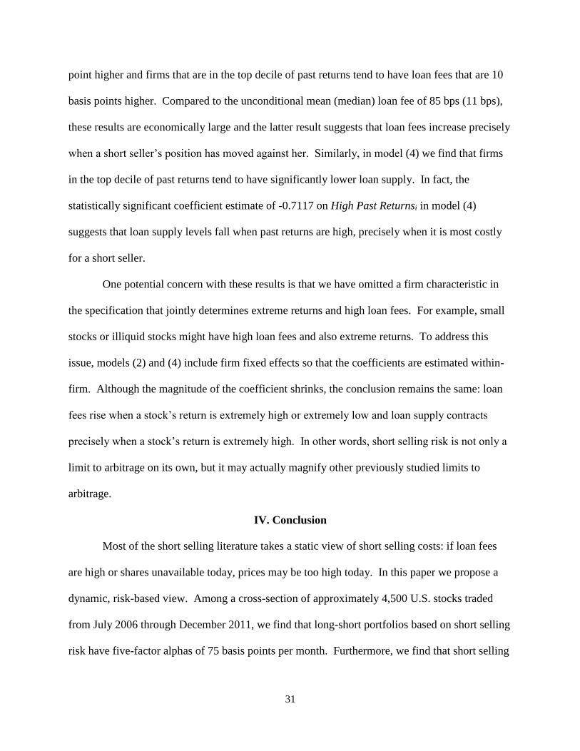
IV. Conclusion
Most of the short selling literature takes a static view of short selling costs: if loan fees
are high or shares unavailable today, prices may be too high today. In this paper we propose a
dynamic, risk-based view. Among a cross-section of approximately 4,500 U.S. stocks traded
from July 2006 through December 2011, we find that long-short portfolios based on short selling
risk have five-factor alphas of 75 basis points per month. Furthermore, we find that short selling

32
risk is associated with decreased price efficiency and less short selling today. Overall, we find
that short selling risk is associated with more mispricing and less short selling, especially for
trades with longer holding periods.
This evidence sheds light on two puzzles in the short selling literature. Specifically,
several papers have shown that high short interest predicts low future returns, and thus it is
puzzling that publicly available short interest data continue to have return predictability. Our
results show that this puzzle is particularly strong among stocks with high short selling risk,
which suggests that dynamic short sale constraints may explain some of the puzzle. Moreover,
the literature finds it puzzling that investors do not short sell stocks in larger amounts. We find
that short sellers trade less when short selling risk is high, which suggests that dynamic short sale
constraints help explain the low level of short selling. Taking the two puzzles together, the
overall idea emerges: when short selling is risky, short sellers are less likely to trade and prices
are too high.

33
REFERENCES
Aggarwal, Reena, Pedro A. C. Saffi, and John Sturgess, 2015, The role of institutional investors
in voting: evidence from the securities lending market, Journal of Finance 70, 2309-
2346.
Ang, Andrew, Robert Hodrick, Yuhang Xing, and Xiaoyan Zhang, 2006, The cross-section of
volatility and expected returns, Journal of Finance 61, 259-299.
Asquith, Paul, Parag A. Pathak, and Jay R. Ritter, 2005, Short interest, institutional ownership,
and stock returns, Journal of Financial Economics 78, 243-276.
Battalio, Robert, and Paul Schultz, 2011, Regulatory uncertainty and market liquidity: the 2008
short sale ban's impact on equity option markets, Journal of Finance 66, 2013-2053.
Beber, Alessandro, and Marco Pagano, 2013, Short-selling bans around the world: evidence from
the 2007–09 crisis, Journal of Finance 68, 343-381.
Beneish, Messod Daniel, Charles M. C. Lee, and Craig Nichols, 2015, In short supply: equity
overvaluation and short selling, Journal of Accounting and Economics 60, 33-57.
Boehmer, Ekkehart, Zsuzsa Huszar, and Brad Jordan, 2010, The good news in short interest,
Journal of Financial Economics 96, 80-97.
Boehmer, Ekkehart, Charles Jones, and Xiaoyan Zhang, 2008, Which shorts are informed?
Journal of Finance 63, 491-527.
Boehmer, Ekkehart, Charles M. Jones, and Xiaoyan Zhang, 2013, Shackling the short sellers: the
2008 shorting ban, Review of Financial Studies 26, 1363-1400.
Cohen, Lauren, Karl B. Diether, and Christopher J. Malloy, 2009, Shorting demand and
predictability of returns, Journal of Investment Management 7, 36-52.
D’Avolio, Gene, 2002, The market for borrowing stock, Journal of Financial Economics 66,
271-306.
D’Avolio, Gene, 2002b, Appendix to “The market for borrowing stock”: Modeling equilibrium,
unpublished manuscript.
D’Avolio, Gene M., and André F. Perold, 2003, Short selling in practice: Intermediating
uncertain share availability, Working Paper.
Danielsen, Bartley, and Sorin Sorescu, 2001, Why do option introductions depress stock prices?
An empirical study of diminishing short sale constraints, Journal of Financial and
Quantitative Analysis 36, 451-484.
Diamond, Douglas W., and Robert E. Verrecchia, 1987, Constraints on short-selling and asset
price adjustment to private information, Journal of Financial Economics 18, 277-311.

34
Diether, Karl B., Kuan-Hui Lee, and Ingrid M. Werner, 2009, It's SHO time! Short-sale price
tests and market quality, Journal of Finance 64, 37-73.
Drechsler, Itmar, and Qingyi Drechsler, 2014, The shorting premium and asset pricing
anomalies, Working Paper.
Duarte, Jefferson, Xiaoxia Lou, and Ronnie Sadka, 2006, Can liquidity events explain the low-
short-interest puzzle? Implications from the options market, Working Paper.
Duffie, Darrell, Nicolae Gârleanu, and Lasse Heje Pedersen, 2002, Securities lending, shorting,
and pricing, Journal of Financial Economics 66, 307-339.
Evans, Richard B., Christopher C. Geczy, David K. Musto, and Adam V. Reed, 2009, Failure is
an option: Impediments to short selling and options prices, Review of Financial Studies
22, 1955-1980.
Fama, Eugene F. and James D. MacBeth, 1973, Risk, return, and equilibrium: Empirical tests,
Journal of Political Economy 81, 607-636.
Fama, Eugene, and Kenneth French, 1993, Common risk factors in the returns on stocks and
bonds, Journal of Financial Economics 33, 3-56.
Fama, Eugene, and Kenneth French, 2008, Dissecting anomalies, Journal of Finance 63, 1653-
1678.
Fama, Eugene, and Kenneth French, 2015, A five-factor asset pricing model, Journal of
Financial Economics 116, 1-22.
Figlewski, Stephen, 1981, The informational effects of restrictions on short sales: Some
empirical evidence, Journal of Financial and Quantitative Analysis 16, 463-476.
Figlewski, Stephen, and Gwendolyn P. Webb, 1993, Options, short sales, and market
completeness, Journal of Finance 48, 761-777.
Geczy, Christopher C., David K. Musto, and Adam V. Reed, 2002, Stocks are special too: An
analysis of the equity lending market, Journal of Financial Economics, 66, 241-269.
Greene, William H., 2002, Econometric Analysis (Prentice-Hall, Upper Saddle River, NJ).
Harrison, Michael J., and David M. Kreps, 1978, Speculative investor behavior in a stock market
with heterogeneous expectations, Quarterly Journal of Economics 92, 323-336.
Hirshleifer, David, Siew Hong Teoh, and Jeff Jiewei Yu, 2011, Do short-sellers arbitrage
accrual-based return anomalies? Review of Financial Studies 24, 2429-2461.
Hou, K., and T. J. Moskowitz, 2005, Market frictions, price delay, and the cross-section of
expected returns, Review of Financial Studies 18, 981-1020.

35
Jones, Charles M., and Owen A. Lamont, 2002, Short-sale constraints and stock returns, Journal
of Financial Economics 66, 207-239.
Jones, Charles, 2008, Shorting restrictions – revisiting the 1930s, Working Paper.
Kolasinski, Adam C., Adam V. Reed, and Matthew C. Ringgenberg, 2013, A multiple lender
approach to understanding supply and search in the equity lending market, Journal of
Finance 68, 559-595.
Lamont, Owen A., 2012, Go down fighting: Short sellers vs. firms, Review of Asset Pricing
Studies 2, 1-30.
Lamont, Owen A., and Jeremy C. Stein, 2004, Aggregate short interest and market valuations,
American Economic Review Papers and Proceedings 94, 29-32.
Lamont, Owen A., and Richard H. Thaler, 2003, Can the market add and subtract? Mispricing in
tech stock carve-outs, Journal of Political Economy 111, 227-268.
Levine, Matt, 2014, What happened to Herbalife yesterday? BloombergView, February 4.
Miller, Edward M., 1977, Risk, uncertainty, and divergence of opinion, Journal of Finance 32,
1151-1168.
Mitchell, Mark, Todd Pulvino, and Erik Stafford, 2002, Limited arbitrage in equity markets,
Journal of Finance 57, 551-584.
Nagel, Stefan, 2005, Short sales, institutional investors and the cross-section of stock returns,
Journal of Financial Economics 78, 277-309.
Newey, Whitney K. and Kenneth D. West, 1987, A simple, positive semi-definite,
heteroskedasticity and autocorrelation consistent covariance matrix, Econometrica 55,
703-708.
Ofek, Eli, Matthew Richardson, and Robert Whitelaw, 2004, Limited arbitrage and short sales
restrictions: Evidence from the options markets, Journal of Financial Economics 74, 305-
342.
Pagan, Adrian, 1984, Econometric issues in the analysis of regressions with generated regressors,
International Economic Review 25, 221-247.
Prado, Melissa Porras, Pedro A. C. Saffi, and John Sturgess, 2014, Ownership structure, limits to
arbitrage and stock returns: Evidence from equity lending markets, Working Paper.
Pontiff, Jeffrey, 2006, Costly arbitrage and the myth of idiosyncratic risk, Journal of Accounting
and Economics 42, 35-52.

36
Rapach, David E., Matthew C. Ringgenberg, and Guofu Zhou, 2016, Aggregate short interest
and return predictability, Journal of Financial Economics 121, 46-65.
Saffi, Pedro A. C., and Kari Sigurdsson, 2011, Price efficiency and short selling, Review of
Financial Studies 24, 821-852.
Senchack Jr., A. J., and Laura T. Starks, 1993, Short-sale restrictions and market reaction to
short-interest announcements, Journal of Financial & Quantitative Analysis 28, 177-194.
Shleifer, Andrei and Robert W. Vishny, 1997, The limits of arbitrage, Journal of Finance 52, 35-
55.
Stambaugh, Robert F., Jianfeng Yu, and Yu Yuan, 2012, The short of it: Investor sentiment and
anomalies, Journal of Financial Economics 104, 288-302.
Stambaugh, Robert F., Jianfeng Yu, and Yu Yuan, 2015, Arbitrage asymmetry and the
idiosyncratic volatility puzzle, Journal of Finance 70, 1903-1948.

37
Panel A: Mean Monthly Portfolio Returns
Panel B: Cumulative Portfolio Returns over Time
Figure 1. Portfolio Returns from Conditioning on Short Selling Risk. Panel A displays mean monthly percentage returns for
portfolios and Panel B plots the cumulative return to long-short portfolios calculated over the period July 2006 through December 2011.
Each month, portfolios are formed by sorting into quintiles using the previous month’s short selling risk and these portfolios are held
for one month. At the far right of the figure in Panel A, we display returns from a long-short portfolio that takes a long position in the
low short selling risk portfolio (quintile 1) and a short position in the high short selling risk portfolio (quintile 5). In Panel B, we plot
the cumulative returns to a long-short portfolio that buys stocks in the lowest quintile of short selling risk and shorts stocks in the highest
quintile of short selling risk. These equal-weighted portfolios are then held for one calendar month.
-0.6
-0.4
-0.2
0.0
0.2
0.4
0.6
0.8
1.0
1.2
Short Risk:
1 (Low)
Short Risk:
2
Short Risk:
3
Short Risk:
4
Short Risk:
5 (High)
Long (1) -
Short (5)
Mea
n M
on
thly
Po
rtf
oli
o R
etu
rn
s
(in
percen
t)
-10
0
10
20
30
40
50
60
70
80
July-2006 July-2007 July-2008 July-2009 July-2010 July-2011
Cu
mu
lati
ve R
etu
rn
(in
%)
Date

38
Panel A: Mean Loan Fee Panel B: Mean Loan Fee Changes
Figure 2. Mean Loan Fees Conditional on Stock Returns over the Previous 20 Days. The figures in Panel A and Panel B plot mean
loan fees and mean loan fee changes, respectively, conditional on stock returns over the previous 20 days. Each day, the stock return
over the previous 20 days (i.e., date t-1, t-20) is ranked into 50 equally sized bins and then the mean loan fee or loan fee change on date
t is calculated for each bin. In each panel the left vertical axis denotes the Loan Fee in basis points per annum. The loan fee measures
the cost of borrowing a stock and is calculated as the difference between the rebate rate for a specific loan and the prevailing market
rebate rate. The rebate rate for an equity loan is the rate at which interest on collateral is rebated back to the borrower. The right vertical
axis shows the mean value of past 20-day returns in each of the 50 return bins, and the horizontal axis shows the 50 return bins.
-60
-40
-20
0
20
40
60
80
0
50
100
150
200
250
300
350
400
450
500
0 5 10 15 20 25 30 35 40 45 50 55 60 65 70 75 80 85 90 95
Past 2
0 D
ay
Retu
rn
(in %
)
Mean
Loan
Fee
(in
BP
S)
Past 20 Day Return Rank
Loan Fee Stock Return
-60
-40
-20
0
20
40
60
80
-0.5
0
0.5
1
1.5
2
2.5
0 5 10 15 20 25 30 35 40 45 50 55 60 65 70 75 80 85 90 95
Past 2
0 D
ay
Retu
rn
(in %
)
Mean
Loan
Fee
Ch
an
ge
(in
BP
S)
Past 20 Day Return Rank
Loan Fee Change Stock Return

39
Panel A: Mean Loan Supply Panel B: Mean Loan Supply Changes
Figure 3. Mean Loan Supply Conditional on Stock Returns over the Previous 20 Days. The figures in Panel A and Panel B plot
mean loan supply and mean loan supply changes, respectively, conditional on stock returns over the previous 20 days. Each day, the
stock return over the previous 20 days (i.e., date t-1, t-20) is ranked into 50 equally sized bins and then the mean loan supply or loan
supply change on date t is calculated for each bin. In each panel the left vertical axis denotes the Active Loan Supply as a percentage of
shares outstanding. The right vertical axis shows the mean value of past 20-day returns in each of the 50 return bins, and the horizontal
axis shows the 50 return bins.
-60
-40
-20
0
20
40
60
80
0
5
10
15
20
25
0 5 10 15 20 25 30 35 40 45 50 55 60 65 70 75 80 85 90 95
Past 2
0 D
ay
Retu
rn
(in %
)
Mean
Act
ive
Loan
Su
pp
ly
(as
a %
of
share
s ou
tsta
nd
ing)
Past 20 Day Return Rank
Loan Supply Stock Return
-60
-40
-20
0
20
40
60
80
-0.07
-0.06
-0.05
-0.04
-0.03
-0.02
-0.01
0
0.01
0.02
0.03
0 5 10 15 20 25 30 35 40 45 50 55 60 65 70 75 80 85 90 95
Past 2
0 D
ay
Retu
rn
(in %
)
Mean
Act
ive
Loan
Su
pp
ly
Ch
an
ge
(as
a %
of
share
s ou
tsta
nd
ing)
Past 20 Day Return Rank
Loan Supply Change Stock Return

40
Table I
Summary Statistics
Table I displays summary statistics. The sample combines equity lending data from Markit with
data from CRSP, Compustat, NYSE TAQ, and OptionMetrics. The sample contains approximately
4,500 U.S. equities over the period July 1, 2006 through December 31, 2011. Panel A displays
the Mean, Median, 1st Percentile, 99th Percentile, and Standard Deviation values of selected equity
lending variables. Loan Supply represents the total number of shares owned by institutions with
lending programs, expressed as a percentage of shares outstanding. Short Interest is the total
quantity of shares that were loaned out as a percentage of shares outstanding. Short Volume is the
natural log of 1 + short volume as a fraction of shares outstanding from TAQ (multiplied by 100
for scaling). Utilization is the quantity of shares loaned out as a percentage of shares available to
be borrowed. Loan Fee, often referred to as specialness, is the cost of borrowing a share in basis
points per annum. Loan Length is the weighted average number of days that loans have been open.
Qty. Failures is the total quantity of shares that were not delivered as scheduled, expressed as a
percentage of shares outstanding. Panel B displays information regarding firm characteristics:
Market Capitalization and Monthly Return are from CRSP. Panel C displays time-series properties
of the lending market. For each firm, we first calculate the time-series summary statistics, and the
table presents the cross-sectional mean of these values. Panel D displays information on our short
selling risk measure as defined in Section II of the text.
Variable Mean Median 1st 99th
Standard
Deviation
Panel A: Lending Market Characteristics
Loan Supply 18.56% 19.28% 0.00% 46.42% 13.17%
Short Interest 4.43% 2.18% 0.00% 27.33% 5.99%
Short Volume 2.16 1.48 0.18 11.50 2.07
Utilization 13.68% 4.13% 0.00% 85.04% 20.15%
Loan Fee 85.13 bps 11.57 bps -12.28 bps 1,479.29 bps 372.67 bps
Loan Length (in days) 81.46 65.00 2.00 373.00 82.61
Qty. Failures 0.36% 0.00% 0.00% 7.27% 3.39%
Panel B: Firm Characteristics
Market Capitalization $3.77B $0.46B $0.01B $62.81B $16.33B
Monthly Return 0.31% 0.26% -33.84% 35.53% 12.45%
Panel C: Time-Series Properties of Lending Market Characteristics
Loan Fee 70.65 bps 49.01 bps 6.75 bps 301.42 bps 68.48 bps
Utilization 21.58% 18.35% 4.00% 72.09% 17.07%
Panel D: Short Selling Risk
Short Risk 4.04 3.63 -0.92 12.11 4.04

41
Table II
Forecasting Model of Future Short Selling Risk This table shows estimates from an OLS panel regression predicting short selling risk using the model:
𝑉𝑎𝑟(𝐿𝑜𝑎𝑛𝐹𝑒𝑒𝑠𝑖,𝑡+1) = α + 𝛽1𝑉𝑎𝑟𝑁𝑒𝑤𝐹𝑒𝑒𝑖,𝑡 + +𝛽2𝑉𝑎𝑟𝑈𝑡𝑖𝑙𝑖𝑧𝑎𝑡𝑖𝑜𝑛𝑖,𝑡 + 𝛽3𝑇𝑎𝑖𝑙𝑁𝑒𝑤𝐹𝑒𝑒𝑖,𝑡 +
𝛽4𝑇𝑎𝑖𝑙𝑈𝑡𝑖𝑙𝑖𝑧𝑎𝑡𝑖𝑜𝑛𝑖,𝑡 + FEi + FirmCharacteristics + 휀𝑖,𝑡+1,
where VarNewFee is the variance of loan fees for new equity loans, VarUtilization is the natural log
of the variance of the ratio of equity loan supply to loan demand (i.e., utilization), and TailNewFee and
TailUtilization are the 99th percentile of a normal distribution using the trailing annual mean and
variance of loan fee and utilization, respectively. FEi indicates a firm fixed effect and
FirmCharacteristics is a vector of time-varying firm characteristics that include the lagged value of
fee risk, the natural log of one plus the number of shares that failed to deliver (as a percentage of shares
outstanding), the natural log of trading volume (as a percentage of shares outstanding), the natural log
of the bid-ask spread (as a fraction of the closing mid-price), the natural log of market capitalization,
the natural log of return volatility (calculated as the standard deviation of daily stock returns each
month), an indicator variable for stocks paying a dividend this month, an indicator variable for stocks
that had an IPO within the previous 90 days, and an indicator variable for stocks with listed options.
t-statistics, calculated using standard errors clustered by firm and date, are shown below the estimates
in italics. *, **, *** denote statistical significance at the 10%, 5%, and 1% levels, respectively.
Explanatory Dependent Variable: Var(LoanFeet+1)
Variables (1) (2) (3)
VarNewFee 0.7680*** 0.7316*** 0.0611***
(24.49) (27.27) (5.42)
VarUtilization 0.1348*** 0.1242*** 0.0151***
(9.50) (9.88) (3.39)
TailNewFee 0.1266*** 0.1244*** 0.0050*
(7.24) (7.49) (1.69)
TailUtilization -0.0929 -0.0568 -0.0160
(-1.60) (-1.06) (-1.28)
Qty. Failures 0.0061** 0.0094***
(2.25) (4.70)
Volume 0.2858*** 0.0813***
(7.12) (6.43)
Bid-Ask 0.1408*** 0.0330***
(7.06) (2.89)
Market Cap -0.6539*** 0.0330
(-6.59) (1.22)
Var(LoanFeet) 0.9100***
(65.42)
Volatility 0.0830***
(2.78)
Dividend Indicator 0.0139
(1.10)
IPO Indicator 0.1533**
(2.06)
Option Indicator -0.0434**
(-2.47)
N 164,811 162,663 162,657
R2 0.82 0.83 0.97
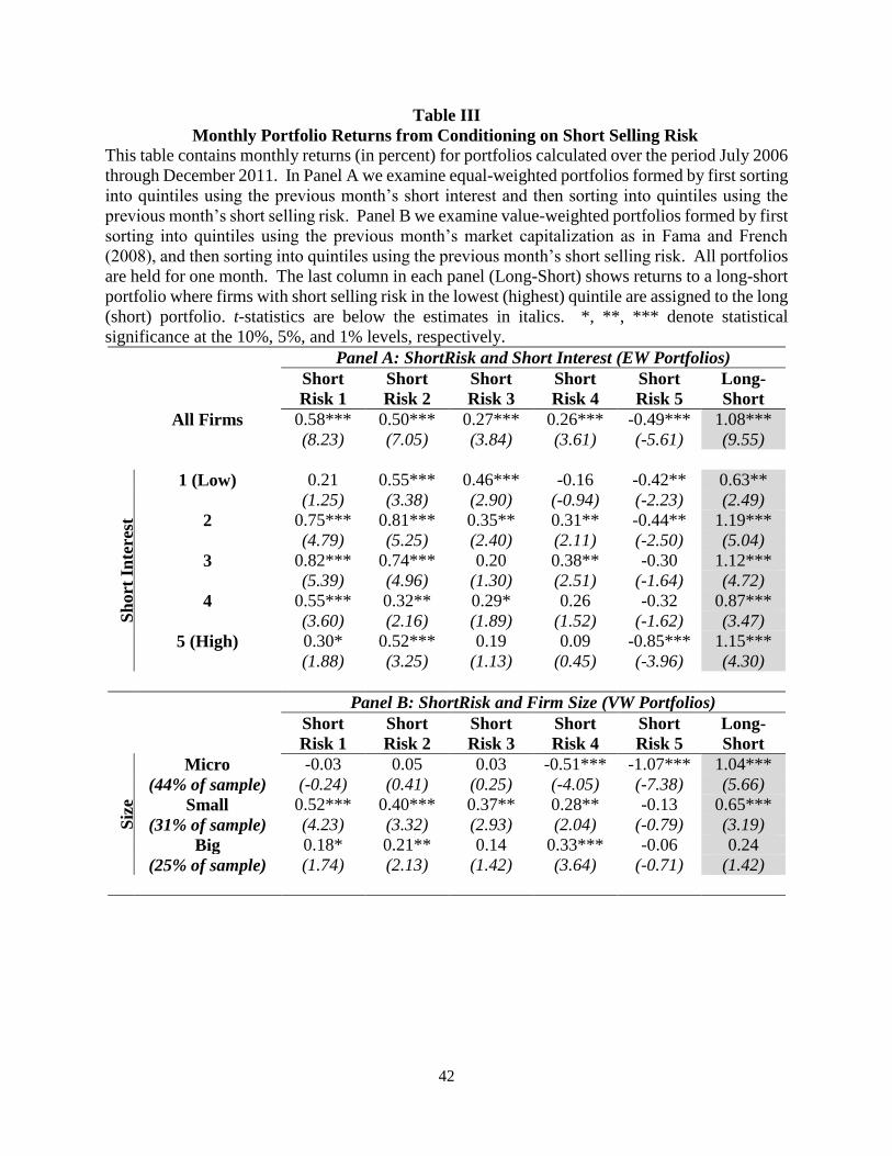
42
Table III
Monthly Portfolio Returns from Conditioning on Short Selling Risk This table contains monthly returns (in percent) for portfolios calculated over the period July 2006
through December 2011. In Panel A we examine equal-weighted portfolios formed by first sorting
into quintiles using the previous month’s short interest and then sorting into quintiles using the
previous month’s short selling risk. Panel B we examine value-weighted portfolios formed by first
sorting into quintiles using the previous month’s market capitalization as in Fama and French
(2008), and then sorting into quintiles using the previous month’s short selling risk. All portfolios
are held for one month. The last column in each panel (Long-Short) shows returns to a long-short
portfolio where firms with short selling risk in the lowest (highest) quintile are assigned to the long
(short) portfolio. t-statistics are below the estimates in italics. *, **, *** denote statistical
significance at the 10%, 5%, and 1% levels, respectively.
Panel A: ShortRisk and Short Interest (EW Portfolios)
Short
Risk 1
Short
Risk 2
Short
Risk 3
Short
Risk 4
Short
Risk 5
Long-
Short
All Firms 0.58*** 0.50*** 0.27*** 0.26*** -0.49*** 1.08***
(8.23) (7.05) (3.84) (3.61) (-5.61) (9.55)
Sh
ort
In
tere
st
1 (Low) 0.21 0.55*** 0.46*** -0.16 -0.42** 0.63**
(1.25) (3.38) (2.90) (-0.94) (-2.23) (2.49)
2 0.75*** 0.81*** 0.35** 0.31** -0.44** 1.19***
(4.79) (5.25) (2.40) (2.11) (-2.50) (5.04)
3 0.82*** 0.74*** 0.20 0.38** -0.30 1.12***
(5.39) (4.96) (1.30) (2.51) (-1.64) (4.72)
4 0.55*** 0.32** 0.29* 0.26 -0.32 0.87***
(3.60) (2.16) (1.89) (1.52) (-1.62) (3.47)
5 (High) 0.30* 0.52*** 0.19 0.09 -0.85*** 1.15***
(1.88) (3.25) (1.13) (0.45) (-3.96) (4.30)
Panel B: ShortRisk and Firm Size (VW Portfolios)
Short
Risk 1
Short
Risk 2
Short
Risk 3
Short
Risk 4
Short
Risk 5
Long-
Short
Siz
e
Micro -0.03 0.05 0.03 -0.51*** -1.07*** 1.04***
(44% of sample) (-0.24) (0.41) (0.25) (-4.05) (-7.38) (5.66)
Small 0.52*** 0.40*** 0.37** 0.28** -0.13 0.65***
(31% of sample) (4.23) (3.32) (2.93) (2.04) (-0.79) (3.19)
Big 0.18* 0.21** 0.14 0.33*** -0.06 0.24
(25% of sample) (1.74) (2.13) (1.42) (3.64) (-0.71) (1.42)
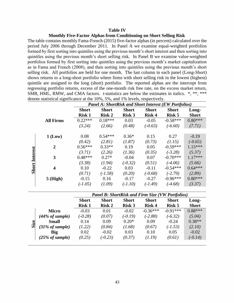
43
Table IV
Monthly Five-Factor Alphas from Conditioning on Short Selling Risk
The table contains monthly Fama-French (2015) five-factor alphas (in percent) calculated over the
period July 2006 through December 2011. In Panel A we examine equal-weighted portfolios
formed by first sorting into quintiles using the previous month’s short interest and then sorting into
quintiles using the previous month’s short selling risk. In Panel B we examine value-weighted
portfolios formed by first sorting into quintiles using the previous month’s market capitalization
as in Fama and French (2008), and then sorting into quintiles using the previous month’s short
selling risk. All portfolios are held for one month. The last column in each panel (Long-Short)
shows returns to a long-short portfolio where firms with short selling risk in the lowest (highest)
quintile are assigned to the long (short) portfolio. The reported alphas are the intercept from
regressing portfolio returns, excess of the one-month risk free rate, on the excess market return,
SMB, HML, RMW, and CMA factors. t-statistics are below the estimates in italics. *, **, ***
denote statistical significance at the 10%, 5%, and 1% levels, respectively.
Panel A: ShortRisk and Short Interest (EW Portfolios)
Short
Risk 1
Short
Risk 2
Short
Risk 3
Short
Risk 4
Short
Risk 5
Long-
Short
All Firms 0.22*** 0.18*** 0.03 -0.05 -0.58*** 0.80***
(3.24) (2.66) (0.48) (-0.63) (-6.60) (7.71)
Sh
ort
In
tere
st
1 (Low) 0.08 0.54*** 0.36* 0.15 0.27 -0.19
(0.42) (2.81) (1.87) (0.73) (1.15) (-0.65)
2 0.56*** 0.33** 0.19 0.05 -0.59*** 1.15***
(3.71) (2.26) (1.36) (0.35) (-3.28) (5.37)
3 0.48*** 0.27* -0.04 0.07 -0.70*** 1.17***
(3.38) (1.94) (-0.32) (0.51) (-4.06) (5.66)
4 0.10 -0.22 0.03 -0.11 -0.54*** 0.64***
(0.71) (-1.58) (0.20) (-0.68) (-2.79) (2.89)
5 (High) -0.15 0.16 -0.17 -0.27 -0.96*** 0.80***
(-1.05) (1.09) (-1.10) (-1.49) (-4.68) (3.37)
Panel B: ShortRisk and Firm Size (VW Portfolios)
Short
Risk 1
Short
Risk 2
Short
Risk 3
Short
Risk 4
Short
Risk 5
Long-
Short
Siz
e
Micro -0.03 0.01 -0.02 -0.36*** -0.91*** 0.88***
(44% of sample) (-0.28) (0.07) (-0.19) (-2.88) (-6.32) (5.04)
Small 0.14 0.09 0.20* 0.09 -0.24 0.38**
(31% of sample) (1.22) (0.84) (1.68) (0.67) (-1.53) (2.10)
Big 0.02 -0.02 0.03 0.10 0.05 -0.02
(25% of sample) (0.25) (-0.23) (0.37) (1.19) (0.61) (-0.14)

44
Table V
Cross-sectional Relation between Monthly Percentage Returns and Short Selling Risk
The table contains Fama and MacBeth (1973) regression results. For each model, we run 63 monthly cross-
sectional regressions of the form:
𝑅𝑒𝑡𝑖,𝑡+1 = α + 𝛽1𝑆ℎ𝑜𝑟𝑡 𝑅𝑖𝑠𝑘𝑖,𝑡 + 𝛽2𝑆ℎ𝑜𝑟𝑡 𝐼𝑛𝑡𝑒𝑟𝑒𝑠𝑡𝑖,𝑡+ Controls + 휀𝑖,𝑡+1,
where Ret is the buy and hold return percent over the subsequent month, excess of the one-month risk-free
rate. ShortRisk is the fitted value from a regression model which forecasts future loan fee variance. Short
Interestt=0 is the quantity of shares borrowed, normalized by shares outstanding; Mispricing is the
mispricing measure from Stambaugh et al. (2015); Market / Book is the log of the market-to-book ratio;
Market Cap is the log of market capitalization lagged by one month; Idio. Volatility is the log of
idiosyncratic volatility from a Fama-French three-factor regression; Bid-Ask is the log of the closing bid-
ask spread; Returnt-1 is the return on each stock lagged by one month; Loan Fee is the cost of borrowing a
share in basis points per annum, and Loan Supply is the total number of shares that are actively available
to be lent (as a fraction of shares outstanding). We report the time-series mean of the parameter estimates
with t-statistics, calculated using a block bootstrap with 500 replications, shown below the coefficient
estimates. *, **, *** denote statistical significance at the 10%, 5%, and 1% levels, respectively.
Dependent Dependent Variable: Monthly Excess Returnt+1
Variable (1) (2) (3)
Short Risk -0.0013*** -0.0008*** 0.0013* (-4.31) (-2.80) (1.91)
Short Interest -0.0020 -0.0042** -0.0049*** (-0.99) (-2.23) (-2.63)
Mispricing 0.0369***
(3.09)
Short Risk × Misp -0.0039***
(-2.74)
Market / Book -0.0080*** -0.0110*** -0.0121*** (-4.58) (-5.31) (-5.95)
Market Cap -0.0030*** -0.0048*** -0.0045***
(-4.88) (-6.41) (-6.07)
Idio. Volatility 0.0026 0.0017 (0.84) (0.62)
Bid-Ask -0.0057*** -0.0054***
(-7.54) (-7.51)
Returnt -0.0204* -0.0316** (-1.71) (-2.42)
Returnt-1 -0.0164* -0.0175*
(-1.92) (-1.93)
Loan Fee -0.0008** -0.0007*
(-2.15) (-1.88)
Loan Supply -0.0001 -0.0000
(-1.09) (-0.52)
Intercept 0.0227 0.0013 -0.0334
(-0.39) (0.06) (-1.60)
N 154,537 149,301 140,815
Average R2 0.10 0.06 0.07

45
Table VI
Price Efficiency and Short Selling Risk This table examines the relation between the Hou and Moskowitz (2005) measure of price
efficiency and short selling risk using OLS panel models of the form:
𝑃𝑟𝑖𝑐𝑒𝐷𝑒𝑙𝑎𝑦𝑖,𝑦= α + 𝛽1𝑆ℎ𝑜𝑟𝑡𝑅𝑖𝑠𝑘 + 𝛽2𝐿𝑜𝑎𝑛𝐹𝑒𝑒 + 𝛽3𝐿𝑜𝑎𝑛𝑆𝑢𝑝𝑝𝑙𝑦 + 𝐶𝑜𝑛𝑟𝑜𝑙𝑠 + 휀𝑖,𝑦,
where the dependent variable, PriceDelay, is the D1 price delay measure from Hou and Moskowitz
(2005). Short Risk is the fitted value from a regression model that forecasts future loan fee
variance. Loan Fee is the mean cost of borrowing a share in basis points per annum, divided by
100 for scale purposes; Loan Supply is the mean total number of shares owned by institutions that
are actively available to be lent (as a fraction of shares outstanding); Qty. Failures is the total
quantity of shares that were not delivered as scheduled; Market Cap. is the log of mean market
capitalization for each firm-year; Volume is the log of mean total trading volume for each firm (as
a fraction of shares outstanding); Bid-Ask Spread is the mean bid-ask spread; Listed Option is an
indicator for whether a stock has listed options. All variables are annual and we include year fixed
effects in all models. t-statistics, calculated using a block bootstrap with 200 replications, are
shown below the coefficient estimates. *, **, *** denote statistical significance at the 10%, 5%,
and 1% levels, respectively.
Explanatory Dependent Variable: Price Delay (D1)
Variable (1) (2) (3)
Short Risk 0.0067*** 0.0072*** 0.0070***
(6.20) (7.32) (6.72)
Loan Supply -0.0068*** -0.0015*** -0.0015***
(-22.75) (-5.47) (-5.48)
Qty. Failures -0.0008 -0.0010
(-0.50) (-0.59)
Market Cap. -0.0212*** -0.0212***
(-10.36) (-10.37)
Volume -0.0099** -0.0098**
(-3.03) (-3.02)
Bid-Ask Spread 0.0546*** 0.0545***
(14.35) (14.33)
Listed Option -0.0118 -0.0120
(-0.29) (-0.32)
Loan Fee 0.0005
(0.52)
Intercept 0.3924*** 1.0344*** 1.0348***
(38.47) (27.22) (27.23)
Year Fixed
Effect
Yes Yes Yes
N 15,662 14,904 14,904
R2 0.20 0.30 0.30

46
Table VII
Relation between Arbitrage, Short Selling Risk, and Time Horizon This table contains OLS panel regression results examining the relation between option mispricing, short selling risk, and the time to option expiration
according to the model:
𝑦𝑖,𝑡 = 𝛽1𝑀𝑜𝑛𝑡ℎ𝑠 𝑇𝑜 𝐸𝑥𝑝𝑖,𝑡 + 𝛽2𝑆ℎ𝑜𝑟𝑡 𝑅𝑖𝑠𝑘𝑖,𝑡−1+ 𝛽3(𝑆ℎ𝑜𝑟𝑡 𝑅𝑖𝑠𝑘𝑖,𝑡−1× 𝑀𝑜𝑛𝑡ℎ𝑠 𝑡𝑜 𝐸𝑥𝑝𝑖,𝑡) + Controls + 𝐹𝐸𝑖 + 𝐹𝐸𝑡 + 휀𝑖,𝑡,
where 𝑦𝑖,𝑡 is Put-Call Disparity in models (1) through (3) and Short Volume in models (4) through (6). Put-Call Disparity is a measure of option mispricing
calculated as the natural log of the ratio of the actual stock price to the option implied stock price as in Ofek, Richardson, and Whitelaw (2004). Short Volume is the number of shares shorted each date, from TAQ, as a fraction of shares outstanding. Months to Expiration is the number of months until the
option expires. Short Risk is the fitted value from a regression model that forecasts future loan fee variance at the horizon of the option contract. Loan Fee
is the mean cost of borrowing a share in basis points per annum, divided by 100 for scale purposes; Option Liquidity is the mean bid-ask spread of the call
and put prices for a given maturity and strike; Stock Liquidity is the stock bid-ask spread; Short Interestt=0 is the quantity of shares borrowed each month
for each firm, normalized by shares outstanding. All models include firm and date fixed effects. t-statistics, calculated using a block bootstrap with 200
replications, are shown below the coefficient estimates. *, **, *** denote statistical significance at the 10%, 5%, and 1% levels, respectively.
Explanatory Dependent Variable: Put-Call Disparity Dependent Variable: Short Volume (%)
Variable (1) (2) (3) (4) (5) (6)
Months to Expiration 0.1215*** 0.0100** 0.0122** -0.0136*** 0.0055 -0.0006
(38.22) (2.06) (2.28) (-2.77) (0.74) (-0.08)
Short Risk 0.0146*** -0.0782*** -0.0348*** -0.0763* -0.0624 -0.0636
(4.81) (-13.36) (-8.64) (-1.74) (-1.45) (-1.48)
Short Risk × Months 0.0302*** 0.0303*** -0.0056*** -0.0055***
(18.93) (18.13) (-3.63) (-3.57)
Loan Fee 0.0019*** 0.0019*** -0.0004 -0.0004
(20.02) (19.90) (-0.73) (-0.71)
Option Liquidity 0.2212*** 0.3455*** -0.4007***
(6.84) (6.12) (-3.94)
Stock Liquidity 0.1517 0.5146** -5.1249
(1.15) (2.29) (-0.94)
Put-Call Disparity 0.0542 0.0768** 0.0765**
(1.52) (2.03) (2.02)
Short Interest 0.0028***
(13.01)
Firm Fixed Effect Yes Yes Yes Yes Yes Yes
Date Fixed Effect Yes Yes Yes Yes Yes Yes
N 5,052,282 5,052,050 5,049,260 1,403,537 1,403,537 1,403,434
R2 0.50 0.52 0.41 0.41 0.41 0.41

47
Table VIII
Loan Market Conditions as a Function of Past 20-Day Returns
This table shows the results from an OLS panel model examining loan fees and loan supply
according to the following model:
LendingMarketConditioni,t = α + β1LowPastReturnsi,t-1,t-20 +β2HighPastReturnsi, t-1,t-20 + εi,t
where Lending Market Conditioni,t is Loan Feesi,t in models (1) and (2) and Loan Supplyi,t in
models (3) and (4), Low Past Returnsit = 1 if firm i had returns in the bottom decile of all firms
from date t-1 to t-20 and = 0 otherwise, and High Past Returnsit = 1 if firm i had returns in the top
decile of all firms from date t-1 to t-20 and = 0 otherwise. We include firm fixed effects in models
(2) and (4) and month-year fixed effects in all models. t-statistics calculated using robust standard
errors clustered by firm and date are shown below the estimates in italics. *, **, *** denote
statistical significance at the 10%, 5%, and 1% levels, respectively.
Explanatory Dependent Variable: Loan Feei,t Dependent Variable: Loan Supplyi,t
Variable (1) (2) (3) (4)
Low Past Returns 0.7009*** 0.1337*** -3.0116*** -0.0508
(24.20) (11.75) (-13.42) (-1.29)
High Past Returns 0.4189*** 0.0953*** -2.8617*** -0.7117***
(25.46) (12.85) (-17.83) (-19.04)
Firm Fixed Effect No Yes No Yes
Time Fixed Effect Yes Yes Yes Yes
N 4,287,629 4,287,629 4,972,250 4,972,250
Adj. R2 0.08 0.62 0.02 0.82
Top Related