


Languages
Pages
Legal


TDT24
Short Introduction to Finite Element
Method
Gagandeep Singh
Contents
1 Introduction 2
2 What Is a Differential Equation? 2
2.1 Boundary conditions . . . . . . . . . . . . . . . . . . . . . . . . . . . . . . 3
2.2 Solution Methods . . . . . . . . . . . . . . . . . . . . . . . . . . . . . . . . 3
2.3 Finite Difference . . . . . . . . . . . . . . . . . . . . . . . . . . . . . . . . 5
2.3.1 Differential Formula . . . . . . . . . . . . . . . . . . . . . . . . . . 5
2.4 Finite Element . . . . . . . . . . . . . . . . . . . . . . . . . . . . . . . . . . 6
2.4.1 Strong Formulation: Possion’s Equation . . . . . . . . . . . . . . . 7
2.4.2 Motivation . . . . . . . . . . . . . . . . . . . . . . . . . . . . . . . . 8
2.4.3 Weak Formulation: Possion’s Equation . . . . . . . . . . . . . . . 8
2.4.4 Advantages of Weak form Compared to Strong Form . . . . . . . 9
3 Basic Steps in FE Approach 9
3.0.5 Approximating the Unknown u . . . . . . . . . . . . . . . . . . . . 9
3.0.6 What is Approximation in FE? . . . . . . . . . . . . . . . . . . . . . 10
3.0.7 Basis Functions . . . . . . . . . . . . . . . . . . . . . . . . . . . . . 11
3.0.8 Basis Functions 2D . . . . . . . . . . . . . . . . . . . . . . . . . . . 13
4 A Practical Example 16
4.1 The Poisson Equation . . . . . . . . . . . . . . . . . . . . . . . . . . . . . 16
4.2 Minimization formulation . . . . . . . . . . . . . . . . . . . . . . . . . . . 16
4.3 Weak formulation . . . . . . . . . . . . . . . . . . . . . . . . . . . . . . . . 17
5 Geometric representation 17
5.1 Element Integral . . . . . . . . . . . . . . . . . . . . . . . . . . . . . . . . 17
5.2 Load Vector . . . . . . . . . . . . . . . . . . . . . . . . . . . . . . . . . . . 19
6 Did we understand the difference between FE and FD? 20
7 Finite Element on GPU 21
1
1 Introduction
In this short report, the aim of which is to introduce the finite element method, a
very rigorous method for solving partial differential equations (PDEs), I will take you
through the following:
• What is a PDE?
• How to solve a PDE?
• Introduce finite difference method
• Introduce finite element method.
• A pratical example using Laplace Equation.
• Fundamental difference from finite difference.
2 What Is a Differential Equation?
Popular science could describe a partial differential equation as a kind of mathemat-
ical divination or fortue-telling. In a PDE, we always have a mathematical expres-
sion describing the relation between dependent and independent variables through
multiplications and partials. Along with this expression we have given initial con-
ditions and boundary requirements. Solution of the PDE can then use this little
information, and give us all the later states of this information. This is just like a
fortuneteller who asks you about some information and tells you what’s going on in
your life. Well, I do not need to tell the difference between a PDE and fortuneteller.
The relation must be something like "true" and the negation of it.
It is not easy to master the theory of partial differential equations. Unlike the the-
ory of ordinary differential equations, which relies on the "fundamental existence
and uniqueness theorem", there is no single theorem which is central to the subject.
Instead, there are separate theories used for each of the major types of partial differ-
ential equations that commonly arise.
Mathematically, a partial differential equation is an equation which contains par-
tial derivatives, such as the (wave) equation
∂u
∂t=
∂2u
∂x2(1)
In Eq (1), variables x and t are independent of each other, and u is regarded as a
function of these. It describes a relation involving an unknown function u of several
independent variables (here x and t)and its partial derivatives with respect to those
variables. The independent variables x and t can also depened on some other vari-
ables, in which case we must carry out the partial derivatives of x and t .
Another simple elliptic model equation is the Poisson Equation, given by
∆u =∇2u =
∂2u
∂x2+∂
2u
∂y2= f , defined on Ω ∈R
2 (2)
2
−1−0.8
−0.6−0.4
−0.20
0.20.4
0.60.8
1
−1−0.8
−0.6−0.4
−0.20
0.20.4
0.60.8
1
0
0.05
0.1
0.15
0.2
Color: u Height: u
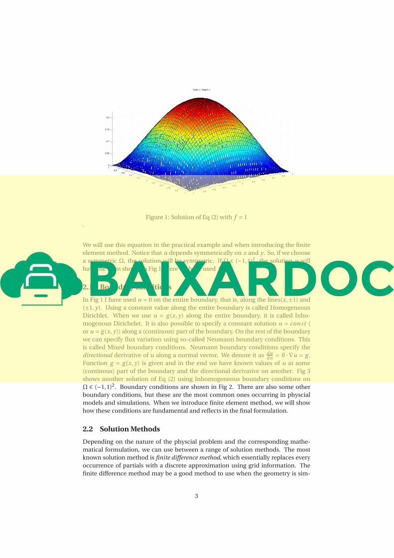
Figure 1: Solution of Eq (2) with f = 1
.
We will use this equation in the practical example and when introducing the finite
element method. Notice that u depends symmetrically on x and y . So, if we choose
a symmetric Ω, the solution will be symmetric. If Ω ∈ (−1,1)2, the solution u will
have the form shown in Fig 1. Here we have used f = 1.
2.1 Boundary conditions
In Fig 1 I have used u = 0 on the entire boundary, that is, along the lines(x,±1) and
(±1, y). Using a constant value along the entire boundary is called Homogeneous
Dirichlet. When we use u = g (x, y) along the entire boundary, it is called Inho-
mogenous Dirichelet. It is also possible to specify a constant solution u = const (
or u = g (x, y)) along a (continous) part of the boundary. On the rest of the boundary
we can specify flux variation using so-called Neumann boundary conditions. This
is called Mixed boundary conditions. Neumann boundary conditions specify the
directional derivative of u along a normal vector. We denote it as dudn
= ~n · ∇u = g .
Function g = g (x, y) is given and in the end we have known values of u at some
(continous) part of the boundary and the directional derivative on another. Fig 3
shows another solution of Eq (2) using Inhomogeneous boundary conditions on
Ω ∈ (−1,1)2. Boundary conditions are shown in Fig 2. There are also some other
boundary conditions, but these are the most common ones occurring in physcial
models and simulations. When we introduce finite element method, we will show
how these conditions are fundamental and reflects in the final formulation.
2.2 Solution Methods
Depending on the nature of the physcial problem and the corresponding mathe-
matical formulation, we can use between a range of solution methods. The most
known solution method is finite difference method, which essentially replaces every
occurrence of partials with a discrete approximation using grid information. The
finite difference method may be a good method to use when the geometry is sim-
3

Figure 2: Boundary conditions on Ω ∈ (−2,2)2
−2−1.5
−1−0.5
00.5
11.5
2
−2.5
−2
−1.5
−1
−0.5
0
0.5
1
1.5
2
−1
0
1
2
3
4
5
6
Color: u Height: u
Figure 3: Solution of Eq (2) using boundary conditions shown in Fig 2
4
ple and not very high accuracy is required. But, when the geometry becomes more
complex, finite difference becomes unreasonably difficult to implement.
The finite element method is conceptually quite different from finite difference when
it comes to the discretization of the PDE, but there are some similarities. It is the
most commonly used method to solve all kinds of PDEs. Matlab has Partial Differ-
ential Equation Toolbox which implements finite element with pre-specified known
PDEs. COMSOL is also based on finite element method.
In the next section, I will mention some few points on finite difference, then go
straight to finite element method. We will then be in a position to discuss some
of the differences between finite difference and finite element.
2.3 Finite Difference
In Eq (2), we have an operator working on u. Let us denote this operator by L. We
can then write
L =∇2=
∂2
∂x2+
∂2
∂y2(3)
Then the differential equation can be written like Lu = f . If for example L = ∇2 −
2∇+2, the PDE becomes ∇2u −2∇u +2u = f . Finite difference methods are based
on the concept of approximating this operator by a discrete operator.
2.3.1 Differential Formula
Let me remind you of Taylor’s formula with the residual part of the functions of two
variables:
u(x +h, y +k) =n∑
m=0
1
m!
(h
∂
∂x+k
∂
∂y
)m
u(x, y)+ rn (4)
where
rn =1
(n+1)!
(h
∂
∂x+k
∂
∂y
)n+1
u(x +θh, y +θk), 0 < θ < 1 (5)
In (4), I have used step lengths h and k in x and y direction, respectively. Let us use
h = k in the following for simplicity. Let us now develop this series of u(x +h, y). I
denote it by um+1,n . The rest follows from it.
um+1,n= um,n
+hum,nx +
h2
2!um,n
xx +h3
3!um,n
xxx +O(h4) (6)
The subscript in ux refers to the partial derivative of u with respect to x. Now, let us
develop the series of um−1,n , um,n+1, and um,n−1.
um−1,n= um,n
−hum,nx +
h2
2!um,n
xx −h3
3!um,n
xxx +O(h4)
um,n+1= um,n
+hum,ny +
h2
2!um,n
y y +h3
3!um,n
y y y +O(h4)
um,n−1= um,n
−hum,ny +
h2
2!um,n
y y −h3
3!um,n
y y y +O(h4)
(7)
5
If we suppose um,nxx is small compared to um,n
x and h → 0, we see from Eq (6) and the
first equation in (7) that
um,nx =
1
h
[um+1,n
−um,n]+O(h) Forward difference
um,nx =
1
h
[um−1,n
−um,n]+O(h) Backward difference
(8)
In the same way, we get
um,ny =
1
h
[um,n+1
−um,n]+O(h) Forward difference
um,ny =
1
h
[um,n−1
−um,n]+O(h) Backward difference
(9)
In the same way, if we suppose um,nxxx is small compared to u
m,nxx and h → 0, we see
from Eq (6) and the first equation in (7) that
um,nxx =
1
h2
[um+1,n
−2um,n+um−1,n
]+O(h2) Central difference (10)
We also get a second order central difference in y from second and third equation in
Eq (7)
um,ny y =
1
h2
[um,n+1
−2um,n+um,n−1
]+O(h2) Central difference (11)
Let us look at Poisson Eq (2). It contains two separate second derivatives, and we
can use Eq (10) and (11) to approximate these with O(h2).
∇2u = uxx +uy y = um,n
xx +um,ny y +O(h2) (12)
This expression gives us the well-known five point formula. One thing this expres-
sion tells us, is that in order to use finite difference methods like this one, we need a
relatively structured grid. Otherwise, we will have difficulties defining the direction
of step length.
In the next section, I will introduce finite element method. I will start from what
is called "point of departure" for the element method.
2.4 Finite Element
One remark that can be made already, is that the finite element method is mathe-
matically very rigorous. It has a much stronger mathematical foundation than many
other methods (It has a more elaborate mathematical foundation than many other
methods), and particularly finite difference. It uses results from real and functional
analysis. I will not touch any of this in this short introduction. We will take the path
of enigneers; forget the mathematical foundation and use the final result.
In the practical example in the end, I have included what we call the minimization
principle. It looks like the one used when deriving the Conjugate gradient method by
minimizing a quadratic function. The answer to this minimization function is our
solution. But there is another result, called Weak formulation, which, when true,
6

Figure 4: The five point stencil for the Possion Equation
also makes the minimization formulation true. So, we will start at the weak formu-
lation and discuss the results we arrive at. I will leave the minimization formulation
in the practical example for those of you who may like minimization principles.
Finite Element (FE) is a numerical method to solve arbitrary PDEs, and to acheive
this objective, it is a characteristic feature of the FE approach that the PDE in ques-
tion is first reformulated into an equivalent form, and this form has the weak form.
2.4.1 Strong Formulation: Poisson Equation
Let us rewrite the Possion Equation stated in the beginning and choose Ω= (0,1)2. I
intend to use only Homogeneous Dirichlet boundary conditions. This gives
∆u =∇2u =
∂2u
∂x2+∂
2u
∂y2= f , defined on Ω= (0,1)2
u(∂Ω) = 0 ∂Ω= (x, y)|x = 0,1 or y = 0,1
(13)
This is called the strong formulation in finite element, and says no more than the
original PDE formulation. Still, there is a reason why we call it strong. We will discuss
everything in terms of strong and weak forms.
7
2.4.2 Motivation
• The Possion problem has a strong formulation; a minization formulation; and
a weak formulation.
• The minimization/weak formulations are more general than the strong for-
mulation in terms of regularity and admissible data.
• The minimization/weak formulations are defined by; a space X , a bilinear
form a and linear form l .
• The minimization/weak formulations identify:
– ESSENTIAL boundary conditions - Dirichlet - reflected in X
– NATURAL boundary conditions - Neumann - reflected in a and l
2.4.3 Weak Formulation: Possion’s Equation
As I wrote, the weak formulation is a re-formulation of the original PDE (Strong
form), and it is from this form that the final FE approach is established. To estab-
lish the weak form of PDE Eq (13), multiply it with an arbitrary function, so-called
weight-function, v(x, y) to obtain
v∇2u = f v (14)
We may even integrate this expression over Ω.
∫
Ω
v∇2u =
∫
Ω
f v (15)
I previously claimed that v(x, y) is arbitrary. This is not completely true, since the
manipulations that v(x, y) undergoes should be meaningful. Let us define a space
of functions and call it H 1
H 1(Ω) =
v : Ω→R :
∫
Ω
v2,
∫
Ω
vx2,
∫
Ω
vy2<+∞
(16)
H 1 is a function space where all the functions are bounded [quadratic integrable].
We want our functions to be well-behaved, so that we can define operations on them
within the rules of (say) integration. Let us now define a sub-space of H 1 where we
can find our solution u. We call this X and
X =
v ∈ H 1(Ω) : v |∂Ω = 0
(17)
Before I explain to you why we have chosen H 1(Ω) as our function space, let us carry
out the integration in Eq (15) a little further. Let u, v ∈ X . We know from calculus that
∇(v∇u) =∇v ·∇u+ v∇2u. We can write
∫
Ω
v∇2u =
∫
Ω
∇(v∇u)−
∫
Ω
∇v ·∇u (18)
Using Gauss’s theorem on ∇(v∇u) we get
∫
Ω
∇(v∇u) =
∫
∂Ω
v︸︷︷︸v |∂Ω=0
∇u · ndS = 0 (19)
8

In Eq (19), we have transformed a surface integral to a line integral and dS refers to
an infinitesimal line segment. I have not put d A on surface integrals, so be aware of
that. Eq (18) now reduces to
∫
Ω
v∇2u =−
∫
Ω
∇v ·∇u (20)
and so, we get
−
∫
Ω
∇v ·∇ud A =
∫
Ω
f vd A (21)
2.4.4 Advantages of Weak form Compared to Strong Form
This equation ((21)) is the final weak formulation. It is equivalent to the strong form
posed above. You can reverse all the steps, and get back to the original equation. Let
me explain the space H 1. Firstly, if you look at the strong form, we have two separate
partial derivatives of u, so the strong form requires that u be continously differen-
tiable until at least second partial derivative. Our new formulations has lowered
this requirement to only first partial derivatives by transforming one of the partial
derivatives onto the weight-function v(x, y). This is the first big advantage of a weak
formulation (now you can guess naming conventions). The subspace X is not diffi-
cult to understand; it is a subspace of H 1 because our weak form requires that the
functions are in H 1; our strong form requires that u be 0 along the boundary, so X is
the subspace of all function which are zero on the boundary. Now remember from
the Motivation section above that I wrote "Dirichlet are essential and reflected in X".
This is automated through using weak form. There are several technical facts about
Dirichlet conditions, but we will let them be.
3 Basic Steps in FE Approach
We are already half-way towards the final formulation [which will be a linear system
Au = b]. These are the steps we follow
• Establish the strong formulation [finished]
• Obtain the weak formulation [finished]
• Choose approximations for the unknown functions, in this case u [next - 1]
• Choose the weight functions v [next - 2]
• Solve the system
3.0.5 Approximating the Unknown u
Let me state our route straight away; the region is divided into smaller parts and the
approximation is carried out over these smaller parts and then, based on these re-
sults, it is established for the entire region. If we split the whole domain into smaller
parts, i.e. finite elements, for which we are able to give an approximtion of u, then
we are able to approximate u for the whole geometry of any form.
So, we say that the "approximation is carried out elementwise", hence the name.
9
Top Related