


Languages
Pages
Legal


SESUG 2012
HW-04
FREQ Out – Exploring Your Data the Old School Way Stephanie R. Thompson, Datamum, Memphis, TN
ABSTRACT
This tried and true procedure just doesn’t get the attention it deserves. But, as they say, it is an oldie but a goodie. Sometimes you just need a quick look at your data and a few simple statistics. PROC FREQ is a great way to get an overview of you data with a limited amount of code. We will explore the basic framework of the procedure to how to customize the output. There will also be an overview of the statistical options that are available.
INTRODUCTION
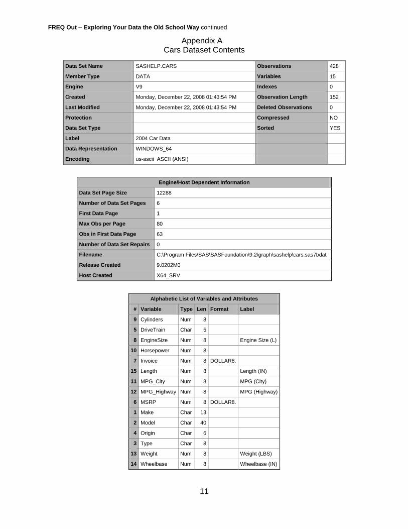
Many times you just need to get a quick look at your data, want to make a fast table, or need to run some simple statistics. The FREQUENCY procedure may be just what you need. This is an easy to learn procedure with a straightforward syntax. In no time at all PROC FREQ may become your go to favorite for quick data checks and statistics. Although it is not designed for generating fancy reports, the output can be used in final documents with the use of ODS. All examples in this paper use the sashelp.cars dataset. This dataset is included with each Base SAS® license and installation. A listing of the contents of cars is included in Appendix A. In this way, you can recreate the examples with ease. The purpose of this paper is to introduce you to PROC FREQ and its capabilities. There is much more that can be done in terms of statistical analysis not covered here. See the links in the References section for more information on what is available in Base SAS and SAS/STAT®.
THE BASICS
PROC FREQ, as is the case with other SAS procedures, will use the last referenced dataset if you do not explicitly list a dataset to use. The bare-bones syntax is below:
proc freq;
run; Running the code above will generate a one-way frequency table for every variable in the dataset. If you have a dataset with a lot of variables or many levels of each variable, the output window will fill up very quickly. The cars dataset generates 48 pages of output. If you want to start the next table immediately after the previous, the compress option is what you need.
proc freq data = sashelp.cars compress;
run;
Explicitly stating the dataset in the procedure calls for the DATA= option. This is necessary if PROC FREQ is the first thing used in your program or if you want to see information about a dataset other than the one most recently used.
proc freq data=sashelp.cars;
run; The next piece of syntax is the tables statement. This statement allows you to specify the tables you want to see in your output. Maybe you are only interested in the variable make in the dataset. You can see it with the code below.
proc freq data=sashelp.cars;
tables make;
run;
FREQ Out – Exploring Your Data the Old School Way continued
2
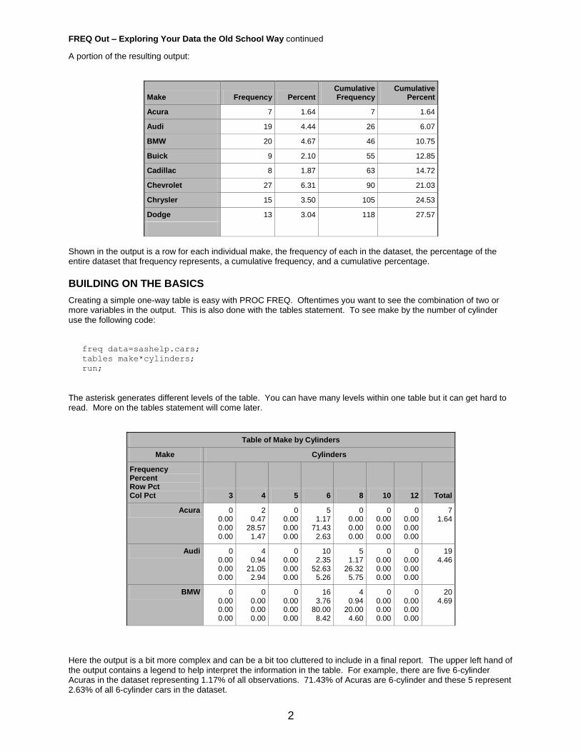
A portion of the resulting output:
Make Frequency Percent Cumulative Frequency
Cumulative Percent
Acura 7 1.64 7 1.64
Audi 19 4.44 26 6.07
BMW 20 4.67 46 10.75
Buick 9 2.10 55 12.85
Cadillac 8 1.87 63 14.72
Chevrolet 27 6.31 90 21.03
Chrysler 15 3.50 105 24.53
Dodge 13 3.04 118 27.57
Shown in the output is a row for each individual make, the frequency of each in the dataset, the percentage of the entire dataset that frequency represents, a cumulative frequency, and a cumulative percentage.
BUILDING ON THE BASICS
Creating a simple one-way table is easy with PROC FREQ. Oftentimes you want to see the combination of two or more variables in the output. This is also done with the tables statement. To see make by the number of cylinder use the following code:
freq data=sashelp.cars;
tables make*cylinders;
run;
The asterisk generates different levels of the table. You can have many levels within one table but it can get hard to read. More on the tables statement will come later.
Table of Make by Cylinders
Make Cylinders
Frequency Percent Row Pct Col Pct 3 4 5 6 8 10 12 Total
Acura 0 0.00 0.00 0.00
2 0.47
28.57 1.47
0 0.00 0.00 0.00
5 1.17
71.43 2.63
0 0.00 0.00 0.00
0 0.00 0.00 0.00
0 0.00 0.00 0.00
7 1.64
Audi 0 0.00 0.00 0.00
4 0.94
21.05 2.94
0 0.00 0.00 0.00
10 2.35
52.63 5.26
5 1.17
26.32 5.75
0 0.00 0.00 0.00
0 0.00 0.00 0.00
19 4.46
BMW 0 0.00 0.00 0.00
0 0.00 0.00 0.00
0 0.00 0.00 0.00
16 3.76
80.00 8.42
4 0.94
20.00 4.60
0 0.00 0.00 0.00
0 0.00 0.00 0.00
20 4.69
Here the output is a bit more complex and can be a bit too cluttered to include in a final report. The upper left hand of the output contains a legend to help interpret the information in the table. For example, there are five 6-cylinder Acuras in the dataset representing 1.17% of all observations. 71.43% of Acuras are 6-cylinder and these 5 represent 2.63% of all 6-cylinder cars in the dataset.

FREQ Out – Exploring Your Data the Old School Way continued
3
Maybe this is too much information about the cars. If you only want to see the frequency and row percentages, you can use table options to turn off some of the output. By default, PROC FREQ gives all four data points for an nxn table.
proc freq data=sashelp.cars;
tables make*cylinders / nopercent nocol;
run;
Table of Make by Cylinders
Make Cylinders
Frequency Row Pct 3 4 5 6 8 10 12 Total
Acura 0 0.00
2 28.57
0 0.00
5 71.43
0 0.00
0 0.00
0 0.00
7
Audi 0 0.00
4 21.05
0 0.00
10 52.63
5 26.32
0 0.00
0 0.00
19
BMW 0 0.00
0 0.00
0 0.00
16 80.00
4 20.00
0 0.00
0 0.00
20
Other common table options are norow (suppressing the row percentages), nocum (suppress cumulative frequency and percentage), and nofreq (suppresses the frequency). Using options helps to create a table that can be inserted into a document and shows only the information you want.
MISSING DATA
So far, we have not seen a table with missing values. How would they show up in the output? By default, missing values are not included in the main table.
Cylinders Frequency Percent Cumulative Frequency
Cumulative Percent
3 1 0.23 1 0.23
4 136 31.92 137 32.16
5 7 1.64 144 33.80
6 190 44.60 334 78.40
8 87 20.42 421 98.83
10 2 0.47 423 99.30
12 3 0.70 426 100.00
Frequency Missing = 2
If you want to see the missing values included in the summary statistics, use the missing tables statement option:
proc freq data=sashelp.cars;
tables cylinders / missing;
run;

FREQ Out – Exploring Your Data the Old School Way continued
4
Cylinders Frequency Percent
Cumulative Frequency
Cumulative Percent
. 2 0.47 2 0.47
3 1 0.23 3 0.70
4 136 31.78 139 32.48
5 7 1.64 146 34.11
6 190 44.39 336 78.50
8 87 20.33 423 98.83
10 2 0.47 425 99.30
12 3 0.70 428 100.00
Choose the option that fits your needs. PROC FREQ makes it easy to see the data as you need to.
BY VALUES OR 3-WAY TABLES?
Maybe you need to see your results grouped by a certain value. Let’s use make as the by variable to see model by number of cylinders. You will need to sort your data first.
proc sort data=sashelp.cars;
by make;
run;
proc freq data=sashelp.cars;
by make;
tables model*cylinders / missing nopercent nocol;
run;
The by statement generates a table for each make and “Make=” proceeds each table.
Make=Acura
Table of Model by Cylinders
Model Cylinders
Frequency Row Pct 4 6 Total
3.5 RL 4dr 0 0.00
1 100.00
1
3.5 RL w/Navigation 4dr 0 0.00
1 100.00
1
MDX 0 0.00
1 100.00
1
NSX coupe 2dr manual S 0 0.00
1 100.00
1
RSX Type S 2dr 1 100.00
0 0.00
1
TL 4dr 0 0.00
1 100.00
1
TSX 4dr 1 100.00
0 0.00
1
Total 2 5 7

FREQ Out – Exploring Your Data the Old School Way continued
5
A three-way table generates slightly different output.
proc freq data=sashelp.cars;
tables make*model*cylinders / missing nopercent nocol;
run;
Table 1 of Model by Cylinders
Controlling for Make=Acura
Model Cylinders
Frequency Row Pct . 3 4 5 6 8 10 12 Total
3.5 RL 4dr 0 0.00
0 0.00
0 0.00
0 0.00
1 100.00
0 0.00
0 0.00
0 0.00
1
3.5 RL w/Navigation 4dr 0 0.00
0 0.00
0 0.00
0 0.00
1 100.00
0 0.00
0 0.00
0 0.00
1
300M 4dr 0 .
0 .
0 .
0 .
0 .
0 .
0 .
0 .
0
300M Special Edition 4dr 0 .
0 .
0 .
0 .
0 .
0 .
0 .
0 .
0
This table has a column for each level of cylinder for the data regardless of whether or not each Make has a value. It is a more comprehensive look at the data but may be more than you need.
LIST ONLY
Sometimes you only want a listing of the data as opposed to a table. PROC FREQ does that too. Just use the list option.
proc freq data=sashelp.cars;
tables model*cylinders / list;
run;
Make Cylinders Frequency Percent Cumulative Frequency
Cumulative Percent
Acura 4 2 0.47 2 0.47
Acura 6 5 1.17 7 1.64
Audi 4 4 0.94 11 2.58
Audi 6 10 2.35 21 4.93
Audi 8 5 1.17 26 6.10
BMW 6 16 3.76 42 9.86
BMW 8 4 0.94 46 10.80
If you want to see the output in descending order by frequency instead of alphabetically by make, use the order=freq procedure option.
proc freq data=sashelp.cars order=freq;
tables model / list;
run;

FREQ Out – Exploring Your Data the Old School Way continued
6
Make Frequency Percent
Cumulative Frequency
Cumulative Percent
Toyota 28 6.54 28 6.54
Chevrolet 27 6.31 55 12.85
Mercedes-Benz 26 6.07 81 18.93
Ford 23 5.37 104 24.30
If you specify a 2-way table, the data is ordered by aggregation of the first variable listed on the tables statement.
proc freq data=sashelp.cars order=freq;
tables model*cylinders / list;
run;
Make Cylinders Frequency Percent Cumulative Frequency
Cumulative Percent
Toyota 6 12 2.82 12 2.82
Toyota 4 14 3.29 26 6.10
Toyota 8 2 0.47 28 6.57
Chevrolet 6 13 3.05 41 9.62
Chevrolet 4 7 1.64 48 11.27
Chevrolet 8 7 1.64 55 12.91
MULTIPLE TABLES
The tables statement is not limited to just one. You can specify any number of tables but all will have the same options if any are specified. If you want tables with different options, use a second tables statement.
proc freq data = sashelp.cars;
tables make model*cylinders model*drivetrain*cylinders / nocol nopercent missing;
run;
proc freq data = sashelp.cars;
tables make / list;
tables model*cylinders model*drivetrain*cylinders / nocol nopercent missing;
run;
If you want to see a single variable contrasted against several others, there are two ways to do this that accomplish the same thing.
proc freq data = sashelp.cars;
tables make*cylinders make*drivetrain make*origin;
run;
proc freq data = sashelp.cars;
tables make*(cylinders drivetrain origin);
run;
QUICK STATISTICS
Since PROC FREQ is used to generate nxn tables, you may want to see if there is a difference in proportions. The chisq table option allows you to do just that.

FREQ Out – Exploring Your Data the Old School Way continued
7
proc freq data = sashelp.cars;
tables origin*drivetrain / nocol nopercent missing chisq;
run;
Table of Origin by DriveTrain
Origin DriveTrain
Frequency Row Pct All Front Rear Total
Asia 34 21.52
99 62.66
25 15.82
158
Europe 36 29.27
37 30.08
50 40.65
123
USA 22 14.97
90 61.22
35 23.81
147
Total 92 226 110 428
Statistics for Table of Origin by DriveTrain
Statistic DF Value Prob
Chi-Square 4 40.1784 <.0001
Likelihood Ratio Chi-Square 4 41.4879 <.0001
Mantel-Haenszel Chi-Square 1 3.5134 0.0609
Phi Coefficient 0.3064
Contingency Coefficient 0.2929
Cramer's V 0.2167
Sample Size = 428
Looking for correlation statistics? Try PLCORR.
Table of Origin by DriveTrain
Origin DriveTrain
Frequency Percent Row Pct Col Pct All Front Rear Total
Asia 34 7.94
21.52 36.96
99 23.13 62.66 43.81
25 5.84
15.82 22.73
158 36.92
Europe 36 8.41
29.27 39.13
37 8.64
30.08 16.37
50 11.68 40.65 45.45
123 28.74
USA 22 5.14
14.97 23.91
90 21.03 61.22 39.82
35 8.18
23.81 31.82
147 34.35
Total 92 21.50
226 52.80
110 25.70
428 100.00
Statistics for Table of Origin by DriveTrain

FREQ Out – Exploring Your Data the Old School Way continued
8
Statistic Value ASE
Gamma 0.1214 0.0569
Kendall's Tau-b 0.0797 0.0374
Stuart's Tau-c 0.0759 0.0357
Somers' D C|R 0.0763 0.0360
Somers' D R|C 0.0831 0.0390
Pearson Correlation 0.0907 0.0430
Spearman Correlation 0.0917 0.0431
Polychoric Correlation 0.1091 0.0605
Lambda Asymmetric C|R 0.0644 0.0447
Lambda Asymmetric R|C 0.1000 0.0423
Lambda Symmetric 0.0847 0.0372
Uncertainty Coefficient C|R 0.0477 0.0143
Uncertainty Coefficient R|C 0.0443 0.0132
Uncertainty Coefficient Symmetric 0.0459 0.0137
Sample Size = 428
PROC FREQ can generate other statistics including AGREE, BINOMIAL, and FISHER. The default value for α is 0.05. You can change it by using the ALPHA= tables statement option. See the online documentation for additional options. If you have SAS/STAT licensed, even more options are available.
GENERATING A DATASET
There may be times you want to create a dataset instead of printed output. PRIC FREQ can do that too. Use the OUTPUT statement with an OUT= to generate a dataset. The noprint option may be useful here since it will suppress all printed output.
proc freq data = sashelp.cars noprint;
tables origin*drivetrain / nocol nopercent missing chisq;
output out=table1 chisq;
run;
The contents of the output dataset (work.table1) are in Appendix B. A statistic must be listed on both the tables and output statements or a warning will be put into the log. If the statistic is missing from the OUTPUT statement without the noprint option, output will be generated but no output dataset. You will see this warning: proc freq data = sashelp.cars;
tables origin*drivetrain / nocol nopercent missing chisq;
output out=table1;
run;
WARNING: No OUTPUT data set is produced because no statistics are requested.
WARNING: Data set WORK.TABLE1 was not replaced because new file is incomplete.
NOTE: There were 428 observations read from the data set SASHELP.CARS.
NOTE: PROCEDURE FREQ used (Total process time):
real time 0.01 seconds
cpu time 0.01 seconds
If the statistic is on the OUTPUT statement but not on the TABLES statement, you will get this warning:

FREQ Out – Exploring Your Data the Old School Way continued
9
proc freq data = sashelp.cars;
tables origin*drivetrain / nocol nopercent missing;
output out=table1 chisq;
run;
WARNING: No OUTPUT data set is produced because no statistics are requested in the
corresponding TABLES statement.
WARNING: Data set WORK.TABLE1 was not replaced because new file is incomplete.
NOTE: There were 428 observations read from the data set SASHELP.CARS.
NOTE: PROCEDURE FREQ used (Total process time):
real time 0.01 seconds
cpu time 0.01 second’
ODS GRAPHICS
Maybe you want to see your data visually instead of in table form. It is very easy wrap your code in an ODS graphics line to generate simple graphics.
ods graphics on;
proc freq data = sashelp.cars;
tables origin*drivetrain / nocol nopercent missing chisq;
run;
ods graphics off;

FREQ Out – Exploring Your Data the Old School Way continued
10
ODS is an easy way to get basic graphs related to the tables you generate. There are other options and types of plots available. Try them out to see what they look like and what may work for you.
REFERENCES
Base SAS® 9.3 Procedures Guide: http://support.sas.com/documentation/cdl/en/procstat/63963/HTML/default/viewer.htm#freq_toc.htm SAS/STAT® 9.3 User's Guide: http://support.sas.com/documentation/cdl/en/statug/63962/HTML/default/viewer.htm#freq_toc.htm
CONCLUSION
After taking a quick look at all that PROC FREQ has to offer, maybe it will find a place in your go to procedures list. The flexible options and simple syntax makes it a fast way to get insight into your data. With a few additional options and statements, you can perform statistical analyses, generate plots, or create a dataset. While PROC FREQ may not be the choice for generating complex reports and tables, it is an easy way to get it done.
CONTACT INFORMATION
Your comments and questions are valued and encouraged. Contact the author at:
Name: Stephanie R. Thompson Enterprise: Datamum Work Phone: 901-326-0030 E-mail: [email protected] Website: www.datamum.com Linked In: Stephanie Thompson, Analytics Professional Twitter: @SRT_SESUG sasCommunity User Name: Stephanie
SAS and all other SAS Institute Inc. product or service names are registered trademarks or trademarks of SAS Institute Inc. in the USA and other countries. ® indicates USA registration.
Other brand and product names are trademarks of their respective companies.
FREQ Out – Exploring Your Data the Old School Way continued
11
Appendix A Cars Dataset Contents
Data Set Name SASHELP.CARS Observations 428
Member Type DATA Variables 15
Engine V9 Indexes 0
Created Monday, December 22, 2008 01:43:54 PM Observation Length 152
Last Modified Monday, December 22, 2008 01:43:54 PM Deleted Observations 0
Protection Compressed NO
Data Set Type Sorted YES
Label 2004 Car Data
Data Representation WINDOWS_64
Encoding us-ascii ASCII (ANSI)
Engine/Host Dependent Information
Data Set Page Size 12288
Number of Data Set Pages 6
First Data Page 1
Max Obs per Page 80
Obs in First Data Page 63
Number of Data Set Repairs 0
Filename C:\Program Files\SAS\SASFoundation\9.2\graph\sashelp\cars.sas7bdat
Release Created 9.0202M0
Host Created X64_SRV
Alphabetic List of Variables and Attributes
# Variable Type Len Format Label
9 Cylinders Num 8
5 DriveTrain Char 5
8 EngineSize Num 8 Engine Size (L)
10 Horsepower Num 8
7 Invoice Num 8 DOLLAR8.
15 Length Num 8 Length (IN)
11 MPG_City Num 8 MPG (City)
12 MPG_Highway Num 8 MPG (Highway)
6 MSRP Num 8 DOLLAR8.
1 Make Char 13
2 Model Char 40
4 Origin Char 6
3 Type Char 8
13 Weight Num 8 Weight (LBS)
14 Wheelbase Num 8 Wheelbase (IN)

FREQ Out – Exploring Your Data the Old School Way continued
12
Sort Information
Sortedby Make Type
Validated YES
Character Set ANSI

FREQ Out – Exploring Your Data the Old School Way continued
13
Appendix B Cars Dataset Contents
Data Set Name WORK.TABLE1 Observations 1
Member Type DATA Variables 13
Engine V9 Indexes 0
Created Sunday, August 19, 2012 01:23:04 PM Observation Length 104
Last Modified Sunday, August 19, 2012 01:23:04 PM Deleted Observations 0
Protection Compressed NO
Data Set Type Sorted NO
Label
Data Representation WINDOWS_64
Encoding wlatin1 Western (Windows)
Engine/Host Dependent Information
Data Set Page Size 12288
Number of Data Set Pages 1
First Data Page 1
Max Obs per Page 117
Obs in First Data Page 1
Number of Data Set Repairs 0
Filename C:\Users\Datamum\AppData\Local\Temp\SAS Temporary Files\_TD5224\table1.sas7bdat
Release Created 9.0202M3
Host Created X64_VSPRO
Alphabetic List of Variables and Attributes
# Variable Type Len Label
6 DF_LRCHI Num 8 DF for Likelihood Ratio Chi-Square
9 DF_MHCHI Num 8 DF for Mantel-Haenszel Chi-Square
3 DF_PCHI Num 8 DF for Chi-Square
1 N Num 8 Number of Subjects in the Stratum
7 P_LRCHI Num 8 P-value for Likelihood Ratio Chi-Square
10 P_MHCHI Num 8 P-value for Mantel-Haenszel Chi-Square
4 P_PCHI Num 8 P-value for Chi-Square
12 _CONTGY_ Num 8 Contingency Coefficient
13 _CRAMV_ Num 8 Cramer's V
5 _LRCHI_ Num 8 Likelihood Ratio Chi-Square
8 _MHCHI_ Num 8 Mantel-Haenszel Chi-Square
2 _PCHI_ Num 8 Chi-Square
11 _PHI_ Num 8 Phi Coefficient
Top Related