![S23 415S23 415 m//e ARMED SERVICES TECHNICAL INFORMATON AGENCY ARLINGTON HALL STATION ARLINGTON 12, VIRGINIA U N C #-AS S ]R FRI E D. NOTICE: When government or other drawings, speci](https://static.fdocuments.in/doc/165x107/60c7b2bad7ea5b7a9c001b6e/s23-415-s23-415-me-armed-services-technical-informaton-agency-arlington-hall-station.jpg)


Languages
Pages
Legal

UNCLASSIFIED
AD 295 9 16
ARMED SERVICES TECHNICAL INFORMATION AGENCYARLINGTON HALL STATIONARLINGTON 12, VIRGINIA
w
UNCLASSIFIED
NOTICE: When government or other drawings, speci-fications or other data are used for any purposeother than in connection with a definitely relatedgovernment procurement operation, the U. S.Government thereby incurs no responsibility, nor anyobligation whatsoever; and the fact that the Govern-ment may have formulated, furnished, or in any waysupplied the said drawings, specifications, or otherdata is not to be regarded by implication or other-wise as in any manner licensing the holder or anyother person or corporation, or conveying any rightsor permission to manufacture, use or sell anypatented invention that may in any way be relatedthereto.
I ERROR STUDY OF ORBITAL PREDICTIONS
J. BoddyandM. Grossberg
Radio Corporation of AmericaAerospace Communications and Controls Division
Burlington, Massachusetts
FINAL REPORT
,C AF 19(604)-8041CR-588-77
20 April 1962
Prepared for
SPO 496L
AIR FORCE COMMAND AND CONTROL DEVELOPMENTDIVISION
AIR RESEARCH AND DEVELOPMENT COMMANDUNITED STATES AIR FORCEBEDFORD, MASSACHUSETTS
.A STIA
FEB 111963 i
J~
'Iuu~"' - i,
IIII
I ERROR STUDY OF ORBITAL PREDICTIONS
J. Boddy andM. Grossberg
I
Radio Corporation of AmericaAerospace Communications and Controls Division
Burlington, Massachusetts
4FINAL REPORT
AF 19(604)-8041j CR-588-77
120 April 1962
[Prepared for
SPO 496L
AIR FORCE COMMAND AND CONTROL DEVELOPMENTDIVISION
AIR RESEARCH AND DEVELOPMENT COMMANDUNITED STATES AIR FORCEBEDFORD, MASSACHUSETTS
1, 1
"Requestb fur additional copies by Agencies of the Department of Defense,
their contractors, and other Government agencies should be directed to the:
ARMED SERVICES TECHNICAL INFORMATION AGENCY
ARLINGTON HALL STATION
ARLINGTON 12, VIRGINIA
Departxent of defense contractors must be established for ASTIA services
or have their 'need-to-know' certified by the cognizant military agency of
their project or contract."
All ot'-er persons and organizations should apply to the:
U. S. DEPARTMENT OF COMMERCE
OFFICE OF TECHNICAL SERVICES
WASHINGTON 25, D. C.
"r
ii
III
TABLE OF CONTENTS
Section Page
FOREWARD ............................. v
ABSTRACT ............................. vi
INTRODUCTION .......................... vii
1 SMOOTHING AND DATA ANALYSIS ............. 1
1.1 DETERMINING OF PARAMETRIC STATISTICS. • • 1
1.Z DIFFERENTIAL CORRECTION ............. 3
1.3 POLYNOMIAL SMOOTHING ............... 7
1.4 AUTOREGRESSIVE SCHEME ............... 13
1.5 EFFECT OF REFERENCE SYSTEM ............. 15
1.6 DATA ANALYSIS ....................... 17
2 ORBITAL COMPUTATIONS AND ERROR BEHAVIOR 27
2.1 OSCULATING ELEMENTS DETERMINATION 28
2.2 PREDICTION DETERMINATION ............ 29
2.3 NUMERICAL ERROR BEHAVIOR OFOSCULATING ELEMENTS ................ 29
3 CONCLUSIONS ........................... 38
REFERENCES ............................... 40
SYMBOLS USED .............................. 42
APPENDIX A - POLAR VERSUS CARTESIAN SMOOTHING • 44
APPENDIX B - DISTORTION OF THE ERRORS ............ 51
APPENDIX C - CONFIDENCE BOUNDS FOR SAMPLECORRELATION COEFFICIENTS AS A TESTFOR RANDOMNESS ................. 57
APPENDIX D - DERIVATION OF THE ORBITALELEMENTS ...................... 62
iii
I
TABLE OF CONTENTS (Continued)
Section Page
D. 1 D.ETERMINATION OF INERTIALCOORDINATES .................... 62
D.. 2 DETERMINATION OF POSITION ANDVELOCITY VECTOR ................ 63
D..3 DETERMINATION OF ORBITAL ELEMENTSELEMENTS ...................... 64
APPENDIX E - THE MOMENTS OF PREDICTED POSITIONERROR FROM MOMENTS OF ORBITALELEMENT ERRORS ................ 68
E. 1 CALCULATION OF INERTIAL GEOCENTRICCOORDINATES FROM ORBITAL PARA-M ETER ......................... 68
E. 2 ERROR ANALYSIS .................. 70
E. 3 EVALUATION OF PARTIAL DERIVATIVESFOR MOMENT FORMULATION ......... 76
iv
III
i LIST OF FIGURES
Figures Page
1-1 Simplified geometric representation for parameterprediction............................24
2 - 1 Standard deviation behavior of orbital elements ofdifferent time spacing ...... .................... 31
2-2 Kurtosis and skewness behavior of eccentricityfor different time spacing ....................... 32
2-3 Kurtosis and skewness behavior of inclinationfor different time spacing ..... ................. 33
2-4 Kurtosis and skewness behavior of semi-majoraxis for different time spacing ..... .............. 34
A-1 Millstone azimuth observations (dashes) and best
fitting fourth degree polynomial (curve) ... ........ 45
A-2 Tapocentric and inertial coordinate systems ..... .. 49
B-1 Ratio of standard deviation of estimated polynomialpoint to standard deviation of observations, versusratio of time from midpoint to half interval, forsecond, third and fourth degree smoothing ....... .. 55
I C-I 90 percent confidence curve for serial correlationcoefficients for various sample - sizes ......... ... 58
1
v
LIST OF TABLES
Table Page
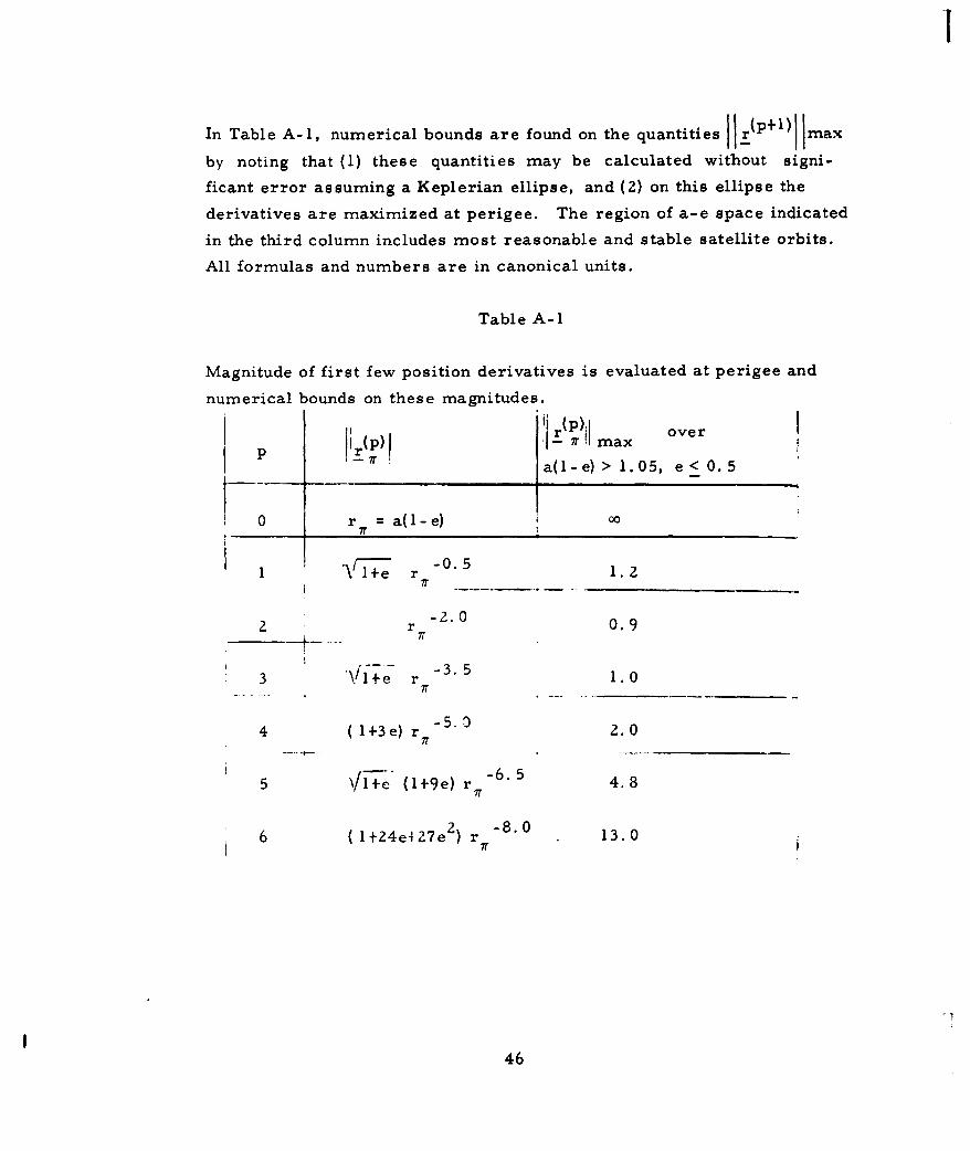
A-I Magnitude of first few position derivati\ es is 46evaluated at perigee and numerical bounds onthese magnitudes.
A-2 2T versus p and (DEV)p. 47
B-i Approximate covariance matrix of midpoint 52polynomial coefficients versus degree ofpolynomial, as a function of number of points, N:
B-2 Ratio of variance of polynomial point to variance 54of observation.
-7
UIIIFOREWORD
The authors are indebted to Dr. P. Nesbeda, under whose direction
this study was conducted, for his assistance and guidance.
The authors are also indebted to Messrs. A. Arcese, H. Chin, J.
Earlam, F. Greco and A. Kaplan for their contributions to this study.IThe assistance of Dr. E. Wahl and Dr. J. Cooley of Space Track for
making available satellite observational data; Dr. J. Arthur of the
Lincoln Laboratories for the use of Millstone Hill Radar data and I.G.
Izsak of the Smithsonian Astrophysical Observatory for the use of Baker-
Nunn data has been greatly appreciated.
1
vii/viii
II
ABSTRACT
This study analyzes the statistics of sensor data obtained from the ob-
servations of artificial satellites. The effect of these statistics on the
estimation of the orbital elements has been evaluated.ISeveral techniques for removal of the actual orbit from the observa-
tions to derive residuals have been investigated. The residuals have
been obtained using both polynomial fitting with and without autoregressive
scheme. From the satellites considered, no consistency was apparent
in the magnitude of the variances of the individual parameters. How-
ever, a consistency was noted in the skewness of the residual. Com-
puter programs have been developed for the determination of the statis-
tics of the orbital elements from observation data. The study shows
that the variances of the orbital elements are functions of the variance
of the observations, the time of observation and description of the mo-
tion of the satellite. Furthermore the variance of any orbital
elements is minimum if the sum of the variance of the observations at
a given time is ininimum for a specific computational procedure of the
orbital element from observations.
The behavior in the statistics of the orbital elements exhibits a consist-
ency in the measure of skewness and excess. Since these quantities are
normalized with respect to the standard deviations it appears that a bias
is introduced in te computation procedure. Thus, the problem of ob-
taining accurate position prediction of artificial satellites is one of
interpl4 between the quality of observations and an analytical description
of the motion of the satellite. How to trade these factors depends upon
the time allowed for deriving the orbit from observations.
ix/x
IIII
INTRODUCTION
This final report summarizes the results of a study on the error of
orbital estimation from observed data performed by the Radio Corpora-
tion of America for SPO 496L Space Track R&D facility under Contract
I AF19(604) -8041.
Determining accurate orbits for an artificial satellite has presented a
new problem in celestial mechanics. To imply that accurate positional
information of an orbiting body can be obtained by more accurate obser-
vation is only partially correct. There is need for an analytical theory
that would represent the motion of the vehicle with an accuracy consis-
tent with the accuracy of the observations.
This study was concerned mainly with the accuracy of the observationsIand their effects on the orbital elements. More specifically, the study
was devoted toI(1) The analysis of the statistics of satellite tracking observations
using data from tracking and surveillance radars and Baker-
Nunn cameras,
(2) The investigations of the statistical and dynamical assumptions
governing the orbit computation based on the Herrick-Gibbs
jmethod and differential correction,
(3) The analysis of the error propagation from observations to
orbital elements following the Herrick-Gibbs method, ;
(4) The investigation of intermixing different types of data and
criteria.
xi
7
Determination of the statistical quality of satellite tracking observations
was conducted by gathering satellite tracking data essentially from the
Millstone Hill Radar and AN/FPS-49. This analysis is contingent on
the removal of the actual orbit from the observations. Several tech-
niques were employed. Section 1 of this report discusses these methods;
namely, simulation, differential correction, and polynomial smoothing
with and without an autoregressive scheme. Each of these methods re-
quires great care in its application, and the statistics gathered should
not be regarded as absolute.
The orbit removal technique depends upon assumptions. To determine
whether the assumptions adequately describe nature, it is necessary to
look at the results of the orbit removal-statistical analysis procedure.
There are two types of tests that may be applied. First, it may be
noted whether the statistics are self-consistent, i. e., is a different
statistical behavior for a given sensor's observations obtained on dif-
ferent satellites?
The second test is the "how well does it work?" type. Since the end
product of the statistical analysis is to be a scheme for precision deter-
mination, estimates of sensor statistics may be used to construct an"optimum estimator, " and to test the orbit so estimated against what-
ever high quality observations are available.
A large number of restrictions are placed on the use of differential
correction. Without drag correction the observational span must be
restricted to a few days, and, in any case, to a few weeks. A very
limited number of observations from each sensor must be used and
the relative quality of observations from different sensors must be
known. Furthermore, a fairly large number of observations is neces-
sary in order to obtain statistically stable residuals.
xii
II
These restrictions, of course, greatly limit the number of satellites
to which this technique can be applied. However, there will probably
be some satellites with sufficient concentration of data. For these
satellites, the amount of computation necessary is large, especially if
the iterative procedure, suggested in subsection 1.2.1, is applied. An
alternative approach to the orbit removal problem is polynomial smooth-
ing which requires much less computation.
The simpler method of polynomial smoothing requires concentrated
data. This method, which has been applied to Millstone data, has been
reasonably successful. However, two procedures must be noted. In
the first place, the observations to be reduced have to be taken over a
time interval limited by the accuracy of the satellite theory. For ex-
ample, if it is desired to analyze range observations from Millstone
which have a standard deviation on the order of one kilometer, then
these observations, plus any others which are used to establish the
orbit, must cover a time span less than that over which the satellite
theory is accurate to, say, one-half kilometer. This time span, even
for a high satellite, is probably not much more than a few days at the
most.
Secondly, using observations from different sensors without properly
weighting them should be avoided. Since the statistical analysis to be
performed is a prerequisite to the determination of weights, it seems
best to perform the correction on observations made by a single sensor.
A disadvantage of the polynomial fitting is that, in the topocentric carte-
sian coordinates, all the parameters are smoothed by a same degree
polynomial. The transformation to cartesian coordinates is an attempt
to obtain uncorrelated residuals. With the autoregressive scheme em-
polyed in conjunction with the polynomial, the smoothing is done directly
on the radar parameters. Each one can then be fitted by a different.
optimum degree of polynomial. The satellite observations handled by
xiii
£
this method indicate that the residuals of the radar parameters were
uncorrelated.
In the process of this investigation it was found that the differential cor-
rection procedure used for astrodynamical data reduction is to be re-
garded as a method of solution of the unweighted least square problem
(Ref. 2). It was also found that the statistics of the residuals exhibit
non-zero third and fourth moments. It can be shown, using the fitting
of observations by a trend and autoregressive scheme, that best esti-
mators for predicting orbital elements can be obtained with independent
estimators of the observations (Ref. 10). Expressions to obtain the
statistics of the osculating elements and error propagation have been
derived analytically. Their usefulness is limited due to the cumbrous
formula. A computer program has been devised to derive the statistics
of the osculating elements. This program utilizes the statistics of the
observations, and the Herrick-Gibbs method. It gives the moments of
the osculating elements.
xivI.
II
SECTION 1
SMOOTHING AND DATA ANALYSIS
To determine the statistical character of electronic or optical observa-
tions of artificial earth satellites, it is necessary to isolate the observa-
tional errors from the "ideal". observations. The observations may be
of slant range, azimuth and elevation, or of right ascension and declina-
tion. Therefore, one must determine, implicitly or explicitly, the true
orbit of the satellite, calculate from this orbit the values which each
sensor should have observed (the ideal observations), and subtract the
ideal from the actual observations to obtain the errors.
The ideal observations may be determined by standard astrodynamical
methods if the satellite's orbit is known. However, in order to use an
orbit to obtain accurate observational errors, it is necessary to know
the orbit with extremely great precision. Since the orbit is usually de-
termined by applying a differential correction reduction on various
observations, certain procedures must be avoided in this reduction or
the "observational errors" obtained become meaningless.
1. 1 DETERMINATION OF PARAMETRIC STATISTICS
1. 1. 1 DESCRIPTION OF METHODS
The inherent statistics associated with any observation parameter ob-
tained from the sensing equipment should be fully understood, together
with a knowledge of their magnitudes, limitations and model assump-
tions presumed.
I 1
I
These statistics could be obtained either from a data analysis study of
a simulated target or from actual satellite observations. Both techniques,
unfortunately, have their own advantages and disadvantages.
1.1.2 SIMULATION STUDY
Parameter statistics are sometimes gathered by means of simulated
targets. For electronic sensors, signals representing those expected
from an actual satellite may be introduced at the front end of the re-
ceiver. When this is done, the orbit removal problem becomes trivial,
for the ideal observations are determined by the "orbit" which was
simulated.
Besides reducing the problem of orbital removal to a purely numerical
one, the technique of target simulation has several other important ad-
vantages. As much statistical data as desired may be gathered, merely
by replaying the target through the sensor-computer system. Further,
the quality of the observations may be calculated as a function of signal
strength. Another important characteristic is that simulation offers
a powerful tool for separating the random and systematic components
of error.
The chief disadvantage of simulation is that one cannot be sure all
sources of error are included. Propagation errors, ground reflections
and target scintillation are usually ignored. Furthermore, special
equipment used for generating the signal may introduce unwanted errors.
In spite of these limitations, it is felt that statistical results gathered
from a sophisticated simulation program should provide enough infor-
mation on the character of observational errors to greatly simplify the
analysis of tracking data. Unfortunately, extensive simulation has
been carried out for very few sensors.
4
1. 1.3 TRACKING DATA ANALYSIS
I To obtain meaningful statistical information from actual satellite obser-
vations, a large number of observations must be available. However,
because of the errors, no possible satellite orbit will exactly satisfy all
of the observations. Thus, in order to estimate the elements of theIorbit, some criterion is needed for closeness of fit of actual and ideal
observations. This criterion is related to the mathematical model
adopted for the errors, in the sense that different models give rise to
different criteria for efficient estimators of the elements, and the dif-
ferent estimators will usually give rise to different sets of observational
residuals. If an error model which does not adequately describe the
character of the errors is used, the residuals obtained will be signifi-
cantly at variance with both the adopted and the true model. The analy-
sis of satellite tracking data may be regarded as an iterative procedure.
In this procedure an orbit is determined which minimizes a criterion
based on the assumed error model and the residuals are tested against
the model. A good first approximation is needed, since "convergence"
is rarely assured.
1. 2 DIFFERENTIAL CORRECTION
11.2.1 DESCRIPTION OF MODEL FOR DIFFERENTIAL CORRECTION
The correct selection of an error model to best describe the character
Iof the errors is extremely important if the residuals are to have signifi-
cant meaning. The simplest error model consists of the following
1 assumptions:
1(1) All observational errors are Gaussian random variables
(2) All errors are uncorrelated
(3) All errors have zero means (observations are unbiased).
3
I
With this model, the most "efficient" estimator is the rigorous least
squares estimator. An exacting discussion on the most "efficient"
estimator is given in Ref. 2. The estimator picks out that orbit which
minimizes the sum of the squares of the weighted residuals, where the
weight for a given residual is the inverse of the standard deviation of
the observational error. To actually compute the orbital element esti-
mates, a nonlinear system of equations must be solved. Differential
correction is an iterative technique for solving these equations. (See
Ref. 1, Z and 3.)
As mentioned,the weights to be used with a differential correction de-
pend upcnthestandard deviations of the errors. Since these standard
deviations are to be obtained by the statistical analysis which follows
the orbit removal, the need of an additional assumption describing the
relative sizes of the error is apparent. This assumption is crucial,
and will be discussed in detail in subsection 1.2.3.
1. 2. 2 THEORETICAL LIMITATIONS OF DIFFERENTIAL CORRECTION
To obtain meaningful residuals, the differential correction procedure
must not introduce theoretical errors, i. e., the correction must select
the true least squares estimate of the orbit to rather high accuracy. In
particular, this requirement imposes the following restrictions on the
procudure:
(1) Quantities derived from observations must be corrected if
their uncertainty gives rise to significant variance in the
residuals
(2) The time span of the observations must be no greater than the
span over which the satellite theory is of "sufficient accuracy"
(3) The loss of accuracy involved in computing partial derivatives
from a Keplerian ellipse assumption must be investigated
4
II
(4) Great care should be taken in the numerical processes, especial-
I ly the matrix inversion.
The first restriction can best be explained by a numerical example. One
effect of atmospheric drag is to reduce the period of a satellite. A typi-
cal value of this reduction is 10 - 8 days per revolution per revolution.
Suppose a preliminary estimate of the drag parameter has been made
which is sufficiently uncertain as to make the value of the period reduc-
tion uncertain up to 10- 9 days/rev2 . This, in turn, causes a variable
time uncertainty whose magnitude is given approximately by 10 "9 times
the square of the number of revolutions from the center time. For two
weeks of observations this amounts to a maximum time error of about
10 - 5 days, hence a maximum position error of about 6 or 7 kilometers.
Such an error is larger than the standard deviation of most observations;
therefore, it is necessary to correct the drag parameter as well as the
orbital elements. Indeed, with an uncertainty of 10 - 9 , drag corrections
are necessary whenever the observations span more than about three
days, or even less time if high-accuracy optical observations are to be
analyzed.
The second restriction refers to the state of the art. If exact initial
conditions of the satellite at some epoch are given and the position of
the satellite can be computed to an accuracy of 0. 2 km for only one
week in the future, then the observational span should be restricted to
about two weeks or less. This restriction, unlike the other three,
cannot be removed by improving the differential correction program.
The third restriction is, perhaps, less important than the others. The
differential correction procedure employs the partial derivatives of
ideal observations with respect to the parameters which are to be cor-
rected. These derivatives may be computed either numerically or
analytically. When analytical differentiation is employed, the
5
I
derivatives are computed on the basis of a two-body Keplerian orbit.
This introduces a second order error into the estimates. The fourth
restriction is self-explanatory.
1.2.3 STATISTICAL LIMITATIONS OF DIFFERENTIAL CORRECTION
The properties which determine the degree of sophistication necessary
in the differential correction program have been examined. The type
of data to be used with the program is analyzed in the light of the as-
sumptions on the error model.
The assumption of Gaussian error distribution is not too critical. Actual
distributions of errors will not differ too much from the Gaussian, and
for these distributions the least squares estimator will still be highly
efficient. The assumptions of unbiased and statistically uncorrelated
observations are more important. If these assumptions are not satis-
fied, and in practice they may not be, the accuracy of the estimated
orbit is greatly reduced. For this reason, whenever there is a sus-
picion of such bias or correlation, the amount of data used from each
pass over each sensor should be restricted to a few points. In this
way, the bias may be treated as an addition to the random error, and
the effects of serial correlation are greatly reduced.
The assumption on the relative quality of observations is critical.
Briefly, the accuracy of an improperly weighted least squares estima-
tion is determined by the more grossly overrated observations. Thus,
if the data include several observations of very poor quality, these
observations must have corresponding low weights attached or they
seriously distort the residuals.
For this reason, if good a priori information on the relative quality of
the observations is not available, the differential correction should be
regarded as an iterative procedure, whereby the residuals are examined
II
to determine new weights for the next correction. Such a procedure
has no guarantee of convergence.
1. 3 POLYNOMIAL SMOOTHING
The technique of polynomial smoothing can be used when compact sets
I of satellite observations are available. The polynomial smoothing con-
sists of finding those time polynomials of a specified degree which best
fit the azimuth, elevation and range parameters in the least square
sense. The polynomial smoothing technique is based on the same as-
sumptions that apply to differential correction. The former technique
gives a less optimum estimate but requires much less computation
than the latter. Polynomial smoothing is applicable only to radar
tracking data, whereas the differential correction technique may be
applied to a wide variety of observations. The observations need not
be taken at equal intervals of time.
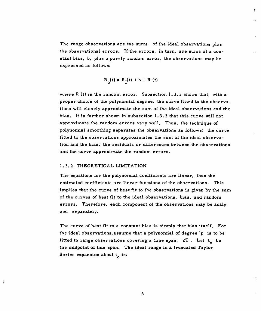
1.3.1 DESCRIPTION OF POLYNOMIAL SMOOTHING
The polynomial smoothing technique consists of finding that poly-
nomial of a given degree which best fits radar observations of a given
type in the least squares sense. For example, to fit radar range with
a second degree polynomial, three quantities - C o , C1 , C2 - must
be found which minimize the expression, S:
1 S(c Cl I C 2 1 (R (t)-C 0 -CI t-C 2 t2 )2 WR(t)2
I twhere R 0 (t) is the observed range at time, t; WR(t) is the inverse of
the standard deviation; and the summation extends over all the obser-
vation times. This problem has a unique solution unless, of course,
there are fewer observations than constants to be determined. The
solution reduces to a linear system of equations. The application of
this technique to the problem of orbit removal is presently discussed.
Ir . 7
The range observations are the sums of the ideal observations plus
the observational errors. If the errors, in turn, are sums of a con-
stant bias, b, plus a purely random error, the observations may be
expressed as follows:
Ro(t) = RI(t) +b +R (t)
where R (t) is the random error. Subsection 1.3. 2 shows that, with a
proper choice of the polynomial degree, the curve fitted to the observa-
tions will closely approximate the sum of the ideal observations and the
bias. It is further shown in subsection 1.3.3 that this curve will not
approximate the random errors very well. Thus, the technique of
polynomial smoothing separates the observations as follows: the curve
fitted to the observations approximates the sum of the ideal observa-
tion and the bias; the residuals or differences between the observations
and the curve approximate the random errors.
1.3.2 THEORETICAL LIMITATION
The equations for the polynomial coefficients are linear, thus the
estimated coefficients are linear functions of the observations. This
implies that the curve of best fit to the observations is given by the sum
of the curves of best fit to the ideal observations, bias, and random
errors. Therefore, each component of the observations may be analy-
zed separately.
The curve of best fit to a constant bias is simply that bias itself. For
the ideal observations, assume that a polynomial of degree 'p is to be
fitted to range observations covering a time span, 2T . Let to be
the midpoint of this span. The ideal range in a truncated Taylor
Series expansion about to is:
8
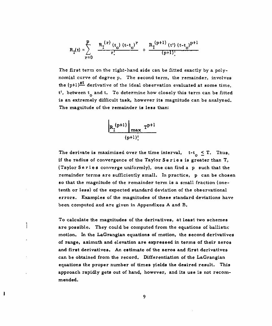
p r) RiPp~l(t~t 0 R t ) (t-to0)r RI(t' () (t-to)0~R1 t)7 '+ (p+l),.r-0
The first term on the right-hand side can be fitted exactly by a poly-
nomial curve of degree p. The second term, the remainder, involvesstthe (p+l)L- derivative of the ideal observation evaluated at some time,
t', between to and t. To determine how closely this term can be fitted
is an extremely difficult task, however its magnitude can be analyzed.
The magnitude of the remainder is less than:
I, I(P+I) I max TP I
(p+l) T
The derivate is maximized over the time interval, t-t < T. Thus,
if the radius of convergence of the Taylor S e r i e s is greater than T,
(Taylor S e r i e s converge uniformly), one can find a p such that the
remainder terms are sufficiently small. In practice, p can be chosen
so that the magnitude of the remainder term is a small fraction (one-
tenth or less) of the expected standard deviation of the observational
errors. Examples of the magnitudes of these standard deviations have
been computed and are given in Appendixes A and B.
To calculate the magnitudes of the derivatives, at least two schemes
are possible. They could be computed from the equations of ballistic
motion. In the LaGrangian equations of motion, the second derivatives
of range, azimuth and elevation are expressed in terms of their zeros
and first derivatives. An estimate of the zeros and first derivatives
can be obtained from the record. Differentiation of the LaGrangian
equations the proper number of times yields the desired result. This
approach rapidly gets out of hand, however, and its use is not recom-
mended.
9
The second scheme is more simple to perform but is subject to
numerical computation errors from an assumed orbit. An approximate
orbit from the record is determined. From this orbit the radar param-
eters at equally spaced time intervals are calculated. The derivatives
of these radar parameters are inferred. Since the orbit used is only
approximate, and the numerical differentiation introduces errors, the
resulting derivatives should be used with a safety factor on the maxi-
mum allowable remainder.
1.3.3 STATISTICAL LIMITATIONS
The polynomial coefficients are computed on the basis of noisy obser-
vations therefore they are subjected to random fluctuations. For the
same reason, the fitted curve is also subjected to fluctuations. If the
fluctuations in the curve are of the same order of magnitude as the
fluctuations in the observations, the residuals will bear little resem-
blance to the observational errors. When d large number of cbcerva-
tions is employed, the fluctuation in the curve becomes quite small.
In Appendixes A and B formulas and graphs for the ratio of the stand-
dard deviation of the curve to the deviation of the observations are
presented as a function of the degree of the polynomial, number of
points, and time. These graphs are derived on the basis of the as-
sumptions that the observations are uncorrelated, stationary, and
equally spaced in time. The non-stationary state of the cartesian
coordinates does not make them strictly applicable, but they are
nevertheless approximately correct.
A numerical example explains the reason the radar coordinate of low-
est standard deviation gives rise to distorted residuals. The following
table shows the true values of the satellite in radar and cartesian co-
ordinates and the radar standard deviations at a particular instant of
time:
10
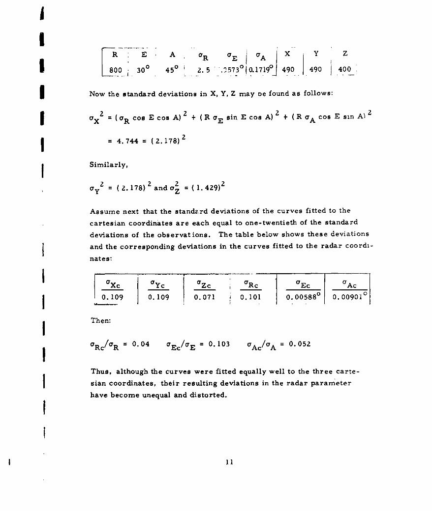
II
R E A, aR a j Ga X Y Z
800 300 450 .. 5 '/ ' °573'1719° 490 490 .400
I Now the standard deviations in X, Y, Z may be found as follows:
aX2 = (a R cos E cos A) 2 + (Ra E sin E cos A) 2 + (R aA cos E sin A 2
= 4.744 = (2.178)2
Similarly,
a 2 = (2.178) 2 and a 2 (1.429)2
Assume next that the standard deviations of the curves fitted to the
cartesian coordinates are each equal to one-twentieth of the standard
deviations of the observations. The table below shows these deviations
I and the corresponding deviations in the curves fitted to the radar coordi-
nates:
Xc Y Zc Rc Ec _Ac
0.109 0.109 0.071 0.101 0.005880 0.009010I{g Then:
a Rc/aR = 0.04 aEc/aE = 0.103 aAc/aA = 0.052
Thus, although the curves were fitted equally well to the three carte-
1 sian coordinates, their resulting deviations in the radar parameter
have become unequal and distorted.I
I 11
1. 3.4 DEGREE OF POLYNOMIAL
A. A Priori
A priori knowledge of the degree of polynomial required to fit a given
set of observations can be obtained from the determination of polynomial
fitting to the true orbital path for the given length of observation time.
Although the true trajectory is unknown, a family of trajectories about
the ideal value can be investigated to determine the optimum degree of
polynomial required. The magnitude of the errors obtained by approxi-
mating the ideal trajectory with any polynomial is indicated in Appendixes
A and B.
For most satellites the Millstone Hill radar parameters can be approxi-
mated by a fourth order polynomial for observation times up to 5-1/2
minutes. Table A-1 in Appendix A indicates the time spread of the amount
of data acceptable for various deviations in the fit of different degree
polynomials to the ideal path of satellite motion.
B. A Posteriori (Orthogonal Polynomials)
Determining the polynomial degree may also be done a posteriori with
the use of orthogonal polynomials. The polynomials are described in
Ref. 4-,Ad only certain properties will be mentioned here.
The most important property of these polynomials is that they may be
used to determine the polynomials of best fit of several different degrees,
with a minimum of duplication. Closely connected with this property is
a simple statistical test (F-test) which may be made on the difference
between the variance of the residuals after fitting polynomials of succes-
sive degrees to the data. In this way, an a posteriori test of the signifi-th ocance of the p order polynomial term may be made.
II
II
Use of orthogonal polynomials has certain computational advantages
I over the usual polynomials. The advantages are most pronounced when
several different polynomial degrees are to be tested. These advantages
g are nullified, if an a priori determination of the degree has been made
or if the observations are not equally spaced in time, or if the observa-
tions are to be weighted unequally.
C. Variate Difference
The technique of applying the variate difference methods to the observa-
tions is considered in detail in Ref. 1. Basically it determines the degree
of the polynomial fit and also estimates the variance of the random com-
ponent by considering the stability of the forward differences of the param-
eters. It;assumes that the radar reports.are comosed of a systematic
and a random.component:
X t -k AtK + t
1k=o
where p is the order of the time polynomial tobe estimated. Estimates
of the variance of the forward differences are obtained. This varianceth
of the random component decreases up to the p difference and then the
f variance should stabilize except for random fluctuations. These random
fluctuations could be due to a harmonic periodicity present in the resi-
Iduals.
1 1.4 AUTOREGRESSIVE SCHEME
The residuals obtained after fitting the optimum degree of polynomial
still exhibit a sinusoidal tendency. It can be shown that the fitting of the
optimum order polynomial plus an autoregressive scheme will better
describe the error process. In addition, this method gives rise to
independence between the observations for the cases considered (Ref. 10)o
13
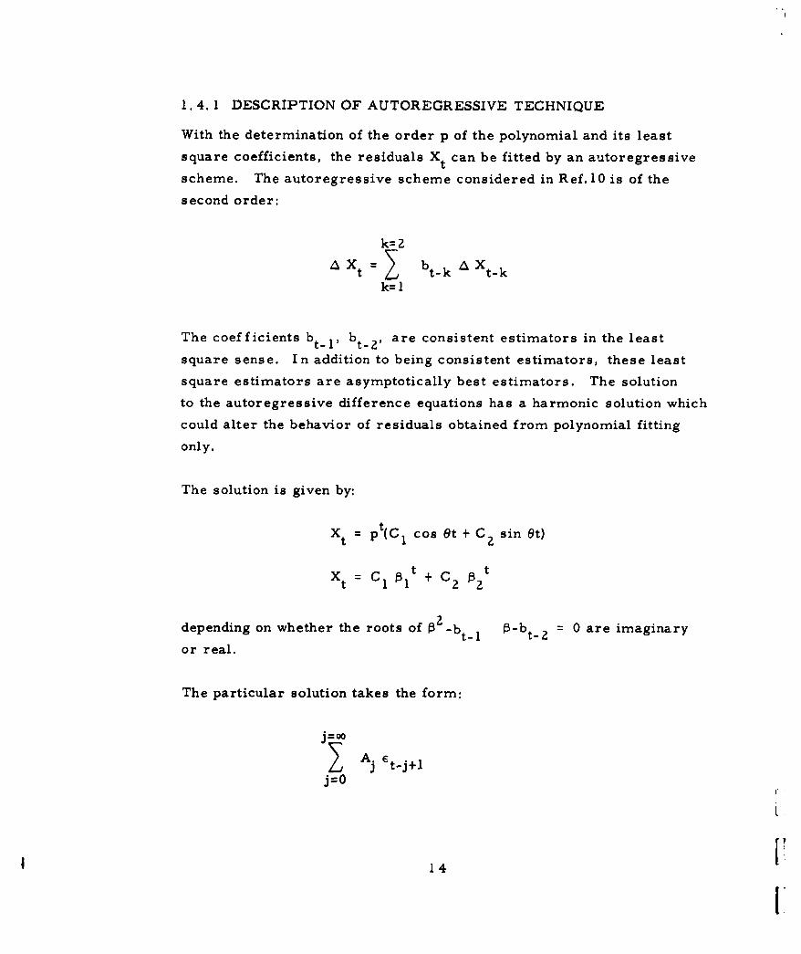
1. 4.1 DESCRIPTION OF AUTOREGRESSIVE TECHNIQUE
With the determination of the order p of the polynomial and its least
square coefficients, the residuals X t can be fitted by an autoregressive
scheme. The autoregressive scheme considered in Ref. 10 is of the
second order:
k= 2
a Xt I bt-k " Xt-kk= 1
The coefficients bt_ 1, bt-Z are consistent estimators in the least
square sense. In addition to being consistent estimators, these least
square estimators are asymptotically best estimators. The solution
to the autoregressive difference equations has a harmonic solution which
could alter the behavior of residuals obtained from polynomial fitting
only.
The solution is given by:
= pt(C1 cos Ot + C, sin Ot)xt t
Xt = C 1 11t + C 22
t
depending on whether the roots of p 2 -b t_ bt 2 0 are imaginary
or real.
The particular solution takes the form:
J A.
j et-j+lj=O
14 [1
i.
so that initially errors are independent. Once introduced into the proc-
ess, they forever exert their influence. For this reason, it was ex-
pected that residuals would be uncorrelated, the dependence tied up in
the initial observations and remaining uncorrelated throughout the proc.-
ess, and therefore tending to diagonalize the covariance matrix. An
estimate of the variance of the autoregressive scheme is
2 2 (1 -b 2 )
Xt "t (1+b2 ) (1-b2 2 - b12)
The residuals after trend and autoregressive fitting were considered
elements of et and assumed to be a stationary process up to second
order. Whereas only the second degree autoregressive scheme is
indicated in Ref. 10, the degree actually required can be estimated
utilizing similar methods to those used to determine the degree of the
polynomial via a variate difference method.
1. 5 EFFECT OF REFERENCE SYSTEM
There are various systems of coordinates in which the observation can
perhaps be smoothed better than in another system. The systems of
radar parameters do not behave like low order polynomials for any
length of time. In order to carry out polynomial smoothing on these
coordinates, it is necessary to resort to polynomials of very high degree -
perhaps, ten or twelve or more for a typical 5-minute pass. It is not
recommended that such high order polynomials be used, as they require
the solution of large scale systems of simultaneous equations. Such
solutions consume much time and storage and are of limited accuracy.
Another objection to high order polynomials is the loss of statistical
stability involved. Furthermore both a priori and a posteriori techni-
ques of estimating polynomial degree become questionable.
15
Two solutions to this problem are known. Either a sequence of functions
may be found (linear and nonlinear) which fit the observations better than
polynomials (autoregressive scheme perhaps) or the observations may be
transformed to a form in which they are easily fitted by polynomials.
Unless differential correction is carried out it seems quite difficult to
measure the truncation errors associated with any smoothing other than
polynomial fitting. Furthermore, most smoothing functions will give
rise to nonlinear systems of equations which will involve a great deal
of machine computation.
1.5.1 POLAR VERSUS TOPOCENTRIC CARTESIAN REFERENCE
SYSTEM
Although the radar coordinates range, elevation and azimuth do not
behave like low order polynomials, the cartesian inertial and the topo-
centric cartesian coordinates of the satellite do. Thus the transforma-
tion from radar to topocentric coordinates produces records which are
very amenable to polynomial smoothing. Appendix A shows that, for ath
wide variety of orbits, the truncation associated with a p degree poly-
nomial is a function only of the time interval, and that for typical radar
data, a fourth degree polynomial is sufficient.
The weights to be used with the cartesian coordinates depend upon the
standard deviations of the radar coordinates. Since these are unknown,
an iterative technique is employed. This technique has been programmed
for the IBM 7090 in Fortran language and performs the following compu-
tations.
Initially the standard deviation in range, azimuth, and elevation, and
the polynomial degree are assumed. The observations are entered and
transformed to cartesian coordinates. Weights for the cartesian coordi-
nates are found on the basis of the assumed radar deviations and the
formulas of linear error propagation. Then normal equations for the
polynomial coefficients are solved, residuals are computed and
16
II
transformed into residuals in range, azimuth, and elevation. The stan-
dard deviations of these residuals are computed and compared with the
assumed values. If the discrepancy is large, the procedure is repeated
starting with the computation of weights, replacing the radar deviations
with the values just computed.
This program has been applied to several records. In all cases, con-
vergence has been achieved after two or three iterations. The final
residuals have not deviated significantly from the Gaussian (subsection
1.6.1). Serial correlations have been small for those coordinates with
relatively large standard deviations, but have been significant when the
deviations are small - usually in elevation. This need not contradict the
hypothesis of statistical independence, due to the poor statistical stability
in these residuals. In general, it isbelievedthat the residuals in those
radar coordinates with large standard deviations are close approximations
to the actual random errors, while, for the other coordinates, the stan-
dard deviations are probably reasonable, but the residuals themselves
are in error. An example of the statistical limitations and distortion of
errors is indicated in subsection 1.3.3.
1.6 DATA ANALYSIS
1.6.1 RADAR DATA FROM MILLSTONE AND MOORES TOWN
Samples of satellite observations from two different sites, Millstone
and the FPS-49 radar at Moorestown, were analyzed to determine the
distribution of the errors, and their correlation. The data supplied by
Moorestown were 10-second radar parameters for various satellites.
These satellites included 1959 Epsilon 1 and Iota 1, 1960 Zeta 1,
Zeta 2, and Nu 2, and 1961 Epsilon 1, Lamba 1, and Omega 1. The
Millstone data were 6-second semi-smoothed radar parameters from
1960 Epsilon 1 and Iota 1. Various degrees of polynomials were fitted
to the transformed cartesian coordinates. The statistics of the resulting
17
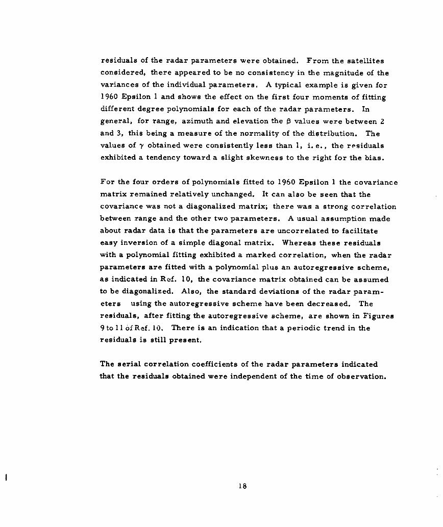
residuals of the radar parameters were obtained. From the satellites
considered, there appeared to be no consistency in the magnitude of the
variances of the individual parameters. A typical example is given for
1960 Epsilon 1 and shows the effect on the first four moments of fitting
different degree polynomials for each of the radar parameters. In
general, for range, azimuth and elevation the 0 values were between 2
and 3, this being a measure of the normality of the distribution. The
values of y obtained were consistently less than 1, i.e., the residuals
exhibited a tendency toward a slight skewness to the right for the bias.
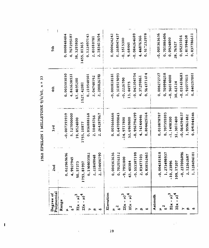
For the four orders of polynomials fitted to 1960 Epsilon 1 the covariance
matrix remained relatively unchanged. It can also be seen that the
covariance was not a diagonalized matrix; there was a strong correlation
between range and the other two parameters. A usual assumption made
about radar data is that the parameters are uncorrelated to facilitate
easy inversion of a simple diagonal matrix. Whereas these residuals
with a polynomial fitting exhibited a marked correlation, when the radar
parameters are fitted with a polynomial plus an autoregressive scheme,
as indicated in Ref. 10, the covariance matrix obtained can be assumed
to be diagonalized. Also, the standard deviations of the radar param-
eters using the autoregressive scheme have been decreased. The
residuals, after fitting the autoregressive scheme, are shown in Figures
9to 11 of Ref. 10. There is an indication that a periodic trend in the
residuals is still present.
The serial correlation coefficients of the radar parameters indicated
that the residuals obtained were independent of the time of observation.
18
~ 4I N -a, 00 ND0 '.000 00 ~ -4 LO It en 00 'D t- c 0 %D 00 -4
V--4 00 , N v O 'o'. 0'. '.0 0 - n %~.0
00 LA)r r- ~ t- 0 N cVn '.0 0 .
o% N 0 Y Ls. (7% - en c A ~ N r N o N
0n 0'0.' NO0~ V~- 1' 0 r ~ N NLnN Lnr-
LA O .N- N OsOLAD oL o w 0 0a% %D0Uo 1-M 0~ O-4~ 0 N cn'o 0 4Ln a - r-o0
M LA
On t- co ene -40n en mIco a' Ln - N -o 0 CLn 0
en0 in O LA 0%t -0 0 1- %0 't r- N 0 %0 0m oo cc 0 o -4 O co LAO I CO -4 N coO 00 1-
0 m~ N - 4 %V o0 N - -4 t- LAO0 a% r- Ir- 0%1 i -1 r- M~mf '.0 LA Co m v Co Co Lns. ' - NJ LA in N4 a, N~ C
On a,0 0 0- 1'0 0 '0 N 0% wNM
'0 .1 ' q%C ;' 0 N N 0 0 v 0n %0 0 0 0 - 0
00 % 0 N - I
0%
01O Co '.0 cn en C'- e%0m 0 14 %D.0 %0 It( '.0 -D a''0. Co m' N 1
a'0 0 - .0a% 'o0 Co 0 m V - - LA OsO0o%0 lW
cno0 0tC V 4 U)C' w. Co Co o VCP- VNN t- Ln-4 V o% -4
0Co t-N0 0 -N t -0'. Da' 0a C 0 r- C, - Voa'cc-
N Z 0 LfLA NN0 0 P-L 0 O0 0V 0 0 0
M 0 "0 .- N 0 a ID 0 0r en a.0
044'-4
0 .0N .N Oa -c t'- '0o0 a, ccVa r -4 ac~s m rf0 a' cncl -Of
a .LA) LAV - %0 (4) o cc 7 a' oco -(n 0' %0 00 ~s0 r- NO -0 %o v
d, m r q0 qLAn %0 -400 V 00'%0 co ak%s0C"-ON a' 1
N0 t-C--4 LA) N re 0 o 71o 0 m m m 0 r-c m t- mf N NN 0% aLAW N N 1 r- r- Ln w w 0 N N N
14-,
0~ 0n a '
E' :JL :L
N4 -d NN~
0 to '0 ( 'oN ?-L' a L'N 'o
19
~%D LA m LA )co LA -4 O0r- " LA o o
0,0 m 0 o0
000 000 % f
ot CY1 O O LAO 0
z 00 0 U" 0-4 N- - VA N0o
o LA)
00NI r-4 L L
r-- -n L
-00 r 00 LA1( 000 r- %0 o 0
C! 0O . 000
uN
mN 00%0 ~ 00 v-L 0
~z4 .T No 000 000
o4 o4 0NI a I'r '
zN 0.-i
0~AI 034 0
F-4 Ln N oo20
1. 6.2 BAKER-NUNN SATELLITE TRACKING CAMERA
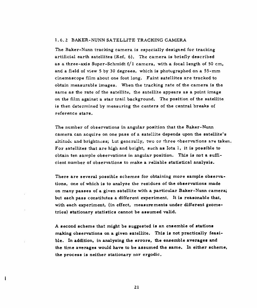
The Baker-Nunn tracking camera is especially designed for tracking
artificial earth satellites (Ref. 6). The camera is briefly described
as a three-axis Super-Schmidt f/l camera, with a focal length of 50 cm,
and a field of view 5 by 30 degrees, which is photographed on a 55-mm
cinemascope film about one foot long. Faint satellites are tracked to
obtain measurable images. When the tracking rate of the camera is the
same as the rate of the satellite, the satellite appears as a point image
on the film against a star trail background. The position of the satellite
is then determined by measuring the centers of the central breaks of
reference stars.
The number of observations in angular position that the Baker-Nunn
camera can acquire on one pass of a satellite depends upon the satellite's
altitudc and brightncss; Lut generally, two or three observations are taken.
For satellites that are high and bright, such as Iota 1, it is possible to
obtain ten sample observations in angular position. This is not a suffi-
cient number of observations to make a reliable statistical analysis.
There are several possible schemes for obtaining more sample observa-
tions, one of which is to analyze the residues of the observations made
on many passes of a given satellite with a particular Baker-Nunn camera;
but each pass constitutes a different experiment. It is reasonable that,
with each experiment, (in effect, measurements under different geome-
tries) stationary statistics cannot be assumed valid.
A second scheme that might be suggested is an ensemble of stations
making observations on a given satellite. This is not practically feasi-
ble. In addition, in analyzing the errors, the ensemble averages and
the time averages would have to be assumed the same. In either scheme,
the process is neither stationary nor ergodic.
21
i
Because one is dealing with an experiment which involves so few sample
points and is devising experiments to increase the sample size,the assump-
tion of stationarity or ergodicity is established. However, this is not Ivalid. The approach taken by the Smithsonian Institute for establishing
accuracies is quite therefore reasonable (Ref. 5).
The accuracies established for the Baker-Nunn camera were determined
as follows: Observations from stations were compared with respect to
a very accurately known orbit and the residues were analyzed.
Two types of data were analyzed: (1) field reduced observations and
(2) precisely reduced observations. The field reduced data are measure-
ments made by the observers at the stations and are subjected to personal
error. The field reduced positions are accurate to within 2-1/2 minutes
of arc in standard deviation and one-tenth second of time in standard
deviation.
Precisely reduced data are field data sent via airmail to the Photo-
reduction Division of the Smithsonian Institute in Cambridge, Massa-
chusetts and analyzed under elaborate laboratory conditions. Precisely
reduced data have an accuracy of two seconds of arc and 0. 001 second
of time in standard deviation.
1.6.3 MULTI-SITE INITIAL WEIGHTING
If an initial knowledge of the variance of the data can be estimated, then
it can be utilized for quicker convergence in the Fortran program for
the polynomial fitting technique as described in subsections 1. 3.4 and
1. 5. 1. The following technique has the advantage of obtaining an esti-
mate of the parameter variance of one site if the parameter statistics
are known for another site. The assumption made is that the variances
are unchanged when subjected to an orthogonal transformation. To carry
out this weighting, it is first necessary to obtain true or expected
22
I
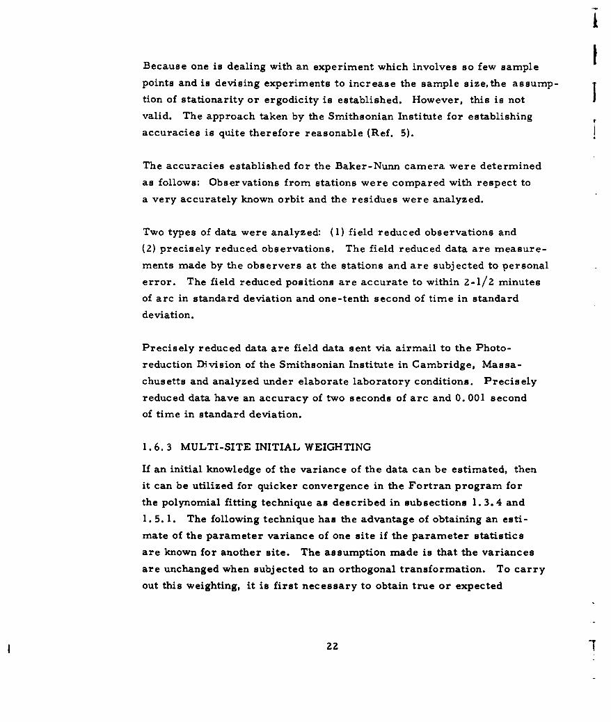
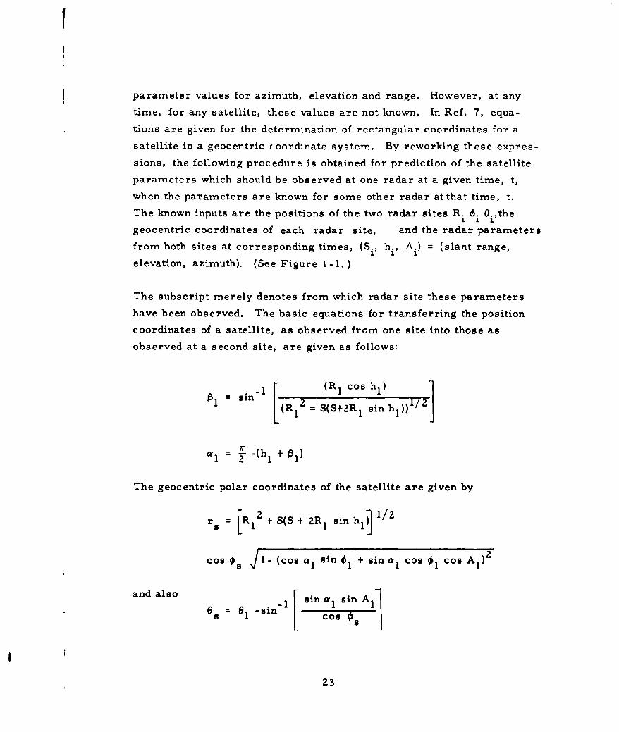
parameter values for azimuth, elevation and range. However, at any
time, for any satellite, these values are not known. In Ref. 7, equa-
tions are given for the determination of rectangular coordinates for a
satellite in a geocentric coordinate system. By reworking these expres-
sions, the following procedure is obtained for prediction of the satellite
parameters which should be observed at one radar at a given time, t,
when the parameters are known for some other radar atthat time, t.
The known inputs are the positions of the two radar sites R. i eithe
geocentric coordinates of each radar site, and the radar parameters
from both sites at corresponding times, (S i , h i , A.) = (slant range,
elevation, azimuth). (See Figure I-1. )
The subscript merely denotes from which radar site these parameters
have been observed. The basic equations for transferring the position
coordinates of a satellite, as observed from one site into those as
observed at a second site, are given as follows:
-sin1 (R 1 cos h1 )
(R[ = S(S+2R 1 sinhl)) I /
a1 = j--(hI +
The geocentric polar coordinates of the satellite are given by
rs = [R1 2 + S(S + 2R 1 sin h1 ] 1/2
cos 4s /1- (cos aI sin + sinaI cos 0I cos A1 )2
and also s0sin sins= Co s
Z3
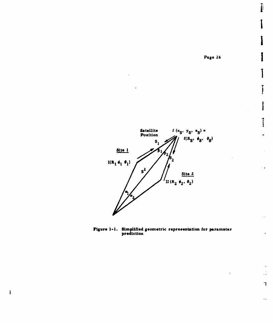
Page 241
Satellite f (X5 1, s s)Position -
1 :O;/ f S 88site I
52 Site 2
U (Rz Oz-e
Figure 1-1. Simplified geometric representation for parameterprediction
I
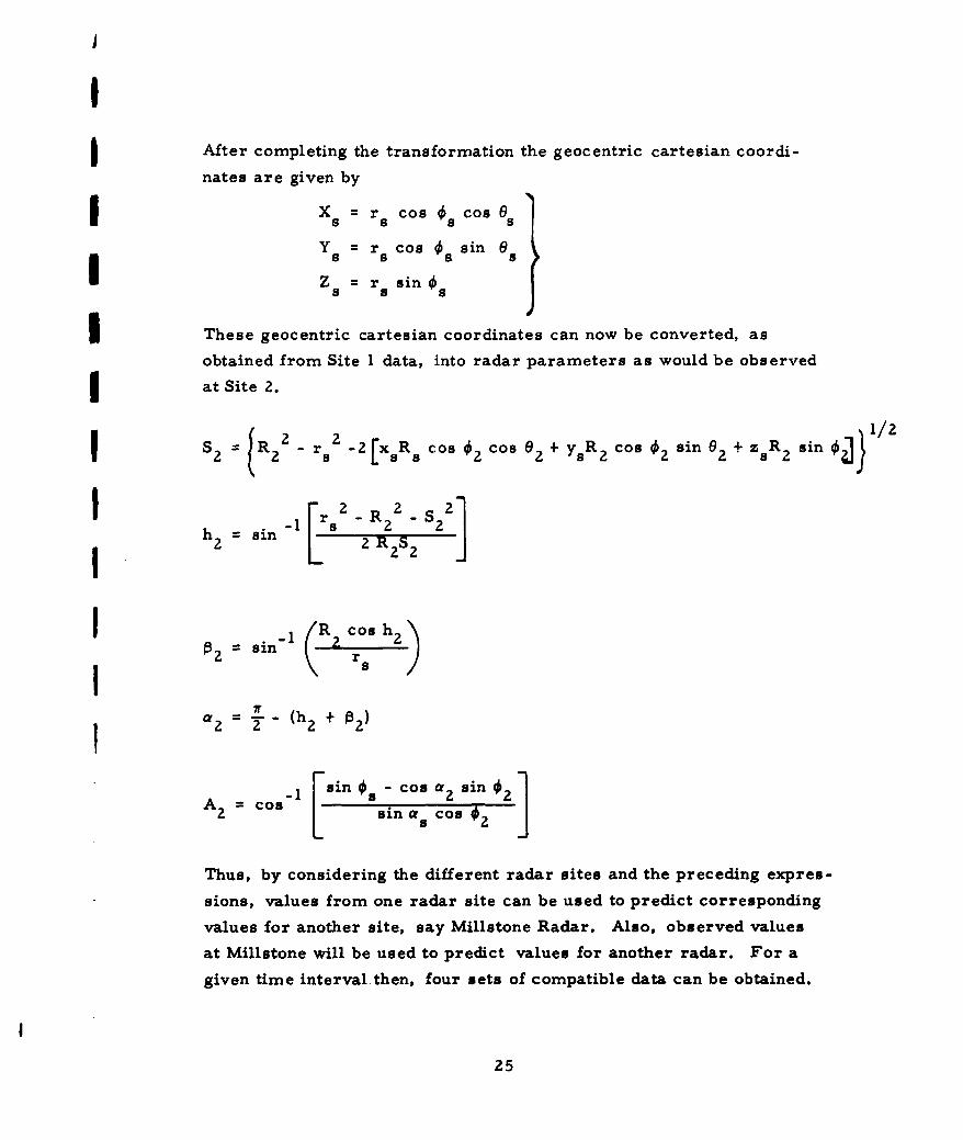
IAfter completing the transformation the geocentric cartesian coordi-
nates are given by
I = r cos Cos 0
Y = r cos sin 6
Z = r sin
These geocentric cartesian coordinates can now be converted, as
obtained from Site I data, into radar parameters as would be observed
I at Site 2.
S =JR2 - r. 2 [xR cos *2cos 02 + ysR2 cos 0?sin 6. + zR sin ~J
h 2 -- sin - irs 2 R 22 - $22]
I.
2 sinrs
a 2 2(h2 + 0 2)
2 cos sin a cos @2
Thus, by considering the different radar sites and the preceding expres-
sions, values from one radar site can be used to predict corresponding
values for another site, say Millstone Radar. Also, observed values
at Millstone will be used to predict values for another radar. For a
given time interval-then, four sets of compatible data can be obtained.
25
iI
For a given time, t, an observed variance S2, can be obtained for these
data. To accomplish this the following information is considered.
It is known that the errors between the observed values and the expected
values are approximately Gaussian distributed, N(O, aR), where R is
observed value and 4 is the expected value.
a2R E([R- - E [R- [R 1)
Thus,
2 ZR-4aR
Thus,
(R- L) is N(O, aR)
For this reason, with S known, bounds on a can be obtained by em-
ploying the X distribution with n-l degrees of freedom given by
x = n S2
a
where n is the sample size.
2
These bounds on a can be used to obtain boundary equations (with an
attached degree of confidence) for polynomial smoothing as discussed in
subsection 1.3. 1.
26
IIII
SECTION 2
ORBITAL COMPUTATIONS AND ERROR BEHAVIOR
Error analysis deals with the type of errors in the prediction and future
ephemeris implied by the expected errors in the sensor data. This con-
cerns the mathematical probability that the vehicle will be in an expected
spacial position at a given time.
Error behavior can be studied as a linear or a nonlinear problem. The
linear analysis is based on assumptions that the errors in the prediction
are linearly related to the errors in the input data. This is realistic if
the standard deviations of the data errors are extremely small and pro-
duce prediction functions with multivariate Gaussian distribution, with
their covariance matrices related by simple matrix multiplication in-
volving partial derivatives of prediction functions with respect to ob-
servations. The way the error analysis is performed depends upon the
distribution of statistics assumed and the dynamical assumptions applied
to the arc of trajectory during the period of observations. The first
section of this report dealt with various techniques for smoothing these
data. This section discusses the error behavior of the osculating ele-
ments and finally the ephemeris.
Statistical assumptions made about the radar parameters are that they
are independent, Gaussian, and can be expanded in a Taylor Series and
truncated after the linear terms without any loss in accuracy. Errors
are also assumed to be non-serially correlated and time invariant.
While several of these assumptions might hold for some radar observa-
tions so that a linear error analysis could be used for the osculating
27
elements, the final elements would certainly not be independent but
would exhibit marked correlation. Some results obtained in the pre-
vious section tend to indicate that most, if not all, of these assumptions
should be considered open to suspicion. The only assumption that seems
to be allowed is that the time of observation is known nearly exact.
2. 1 OSCULATING ELEMENTS DETERMINATION
The initial point of the study of error behavior is the conversion of
three smoothed vectors into one smoothed midpoint velocity vector by
a method attributed to Herrick-Gibbs. This technique is employed by
Space Track for the conversion of radar data (Ref. 7).
An alternative method is to obtain the velocity vector directly from the
radar data. One of the useful by-products of the topocentric polynomial
smoothing is a measure of the midpoint three components of velocity
as coefficients of the first order terms in the polynomial and the accel-
eration as the second order terms. The statics of this velocity are also
easly available. Now that a position and a velocity vector are both
known for a common time, the osculating elements can be uniquely
determined (see Appendix D).
The smoothed radar data exhibited a certain amount of skewness and
non-normality and the radar parameters were definitely not independent.
There appears to be no serial correlation of the parameters and it was
not ascertained whether the covariances were time invariant. With this
knowledge of the statistics of radar smoothed data it was decided to in-
vestigate the error behavior of the osculating elements (1) on the basis
of linear independent errors and (Z) on error behavior in which the first
four moments of the input data were known with their cocumulants.
The radar parameters were expanded in a Taylor Series about their
means and the series truncated at fourth order terms. The method of
propagation of errors was similar to that of Ref. 11. It quickly became
28
obvious that this was an unrewarding tedious task. The procedure was
reduced to only the first two moments and the covariance. The neces-
sary partial derivatives and formulas for the error prediction of the
osculating elements are indicated in Appendix E.
2.2 PREDICTION DETERMINATION
Error behavior of the final prediction was analyzed in Appendix E by
a method similar to that employed to compute the osculating element.
errors. The results obtained from the analysis of several satellites
indicated that the osculating elements were strongly correlated and
were not Gaussianly distributed (see subsection 2. 3). Error propaga-
tion for the first four moments was carried out to evaluate the four
moments of the cartesian coordinates but the covariance was approxi-
mated to second moments only. Only the first partial differentiations
were carried out in Appendix E due to their lengthy nature. All of the
partial derivatives have a periodic tendency which is non-decreasing
with time. The main fault of lengthy prediction time is due to the par-
tial derivatives of the spatial position with respect to the semi-major
axis 8r/8a.
Although this derivative was also periodic, the magnitude of this period
increased with time. When higher order derivatives are considered
they will be increasing with higher orders of time. Thus, prediction
error will increase with time. It might be predominant compared with
the errors introduced when considering a simple Keplerian system,
ignoring the effects caused by earth's oblateness, drag and several
other second order effects on the satellite.
2.3 NUMERICAL ERROR BEHAVIOR OF OSCULATING ELEMENTS
Samples of Millstone 6-second radar data for three different satellites
were subjected to the Herrick-Gibbs technique to determine a series
of midpoint velocity vectors throughout the observation time and, thence,
29
i
the resulting osculating elements. Time spacing between each of the
three -position vectors selected for the Herrick-Gibbs technique was
varied from 6 to 60 seconds. This increase in the time interval con-
siderably reduced the variation of the midpoint velocity. The velocity
vector iscomputed from three weighted position vectors, the weights
beingH.
1d=Gi + --yYi
The time spacing is such that G. is orders of magnitude greater than31
H./y. which is the component that considers the effect of the Keplerian1 1
motion. Since both G. and H. are functions of time, this magnitude dif-1 1
ference can be reduced by increasing the time spacing. The longest
time spacing indicated from the Millstone sample data is approximately
four minutes and even with this length of time, the G. term suppresses
the Keplerian motion effect of Hi/yi 3 .*
The osculating elements were then fitted with unweighted polynomials,
the order of which was predetermined by the variate difference method
and the statistics of the residuals of these osculating elements were
derived. The complete computation procedure from radar parameters
- osculating elements - selection of degree of polynomial and statistics
of residuals has been programmed for the IBM 7090 in Fortran language.
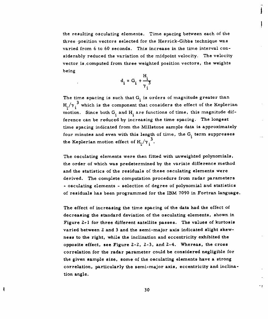
The effect of increasing the time spacing of the data had the effect of
decreasing the standard deviation of the osculating elements, shown in
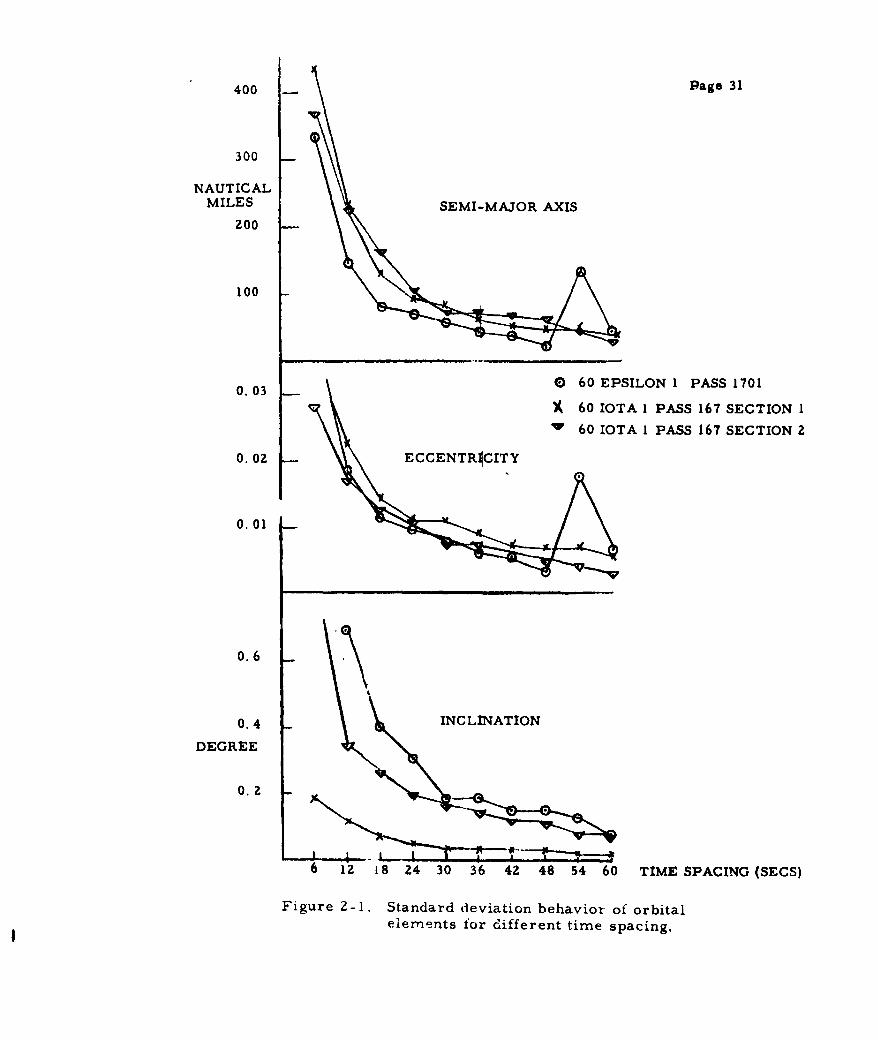
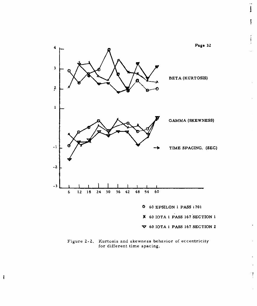
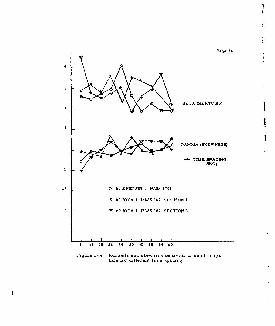
Figure Z-1 for three different satellite passes. The values of kurtosis
varied between 2 and 3 and the semi-major axis indicated slight skew-
ness to the right, while the inclination and eccentricity exhibited the
opposite effect, see Figure 2-2, 2-3, and 2-4. Whereas, the cross
correlation for the radar parameter could be considered negligible for
the given sample size, some of the osculating elements have a strong
correlation, particularly the semi-major axis, eccentricity and inclina-
tion angle.
30
400 Page 31
300
NAUTICALMILES SEMI-MAJOR AXIS
200
100
0. 03 0 60 EPSILON I PASS 170160 IOTA PASS 167 SECTION 1
) 60 IOTA 1 PASS 167 SECTION 2
0. 02 ECCENTRICITY
0.01
0.6
0. 4 INCLINATION
DEGREE
0.2
6 12 18 24 30 36 42 48 54 60 TIME SPACING (SECS)
Figure 2-1. Standard deviation behavior of orbitalelements for different time spacing.
I
I
4 Page 32
3
BETA (KURTOSIS)
GAMMA (SKEWNESS)
-1 + TIME SPACING. (SEC)
-2
-3 I t , I I I I I
6 12 18 24 30 36 42 48 54 60
o 60 EPSILON I PASS 1701
X 60 IOTA I PASS 167 SECTION 1
V 60 IOTA I PASS 167 SECTION 2
Figure 2-2. Kurtosis and skewness behavior of eccentricityfor different time spacing.
/ A
/ Page 33
4 I
3
2BETA (KURTOSIS)
1
GAMMA (SKEWNESS)
.e TIME SPACING. (SEC)
-1
-2
-3 D 60 EPSILON 1 PASS 1701
' 60 IOTA I PASS 167 SECTION I
60 IOTA I PASS 167 SECTION 2i i i .I I 1 _± _ ,
6 12 18 24 30 36 42 48 54 60
Figure 2-3, Kurtosis and skewness behavior of inclinationfor di rent time spacing.
ii
Page 34
44
3
2 BETA (KURTOSIS)
1 *1
GAMMA (SKEWNESS)
- TIME SPACING.(SEC)
-2 o 60 EPSILON I PASS 1701
X 60 IOTA 1 PASS 167 SECTION 1
-3 V 60 IOTA I PASS 167 SECTION 2
6 12 18 24 30 36 42 48 54 60
Figure 2-4. Kurtosis and skewness behavior of semi-majoraxis for different time spacing
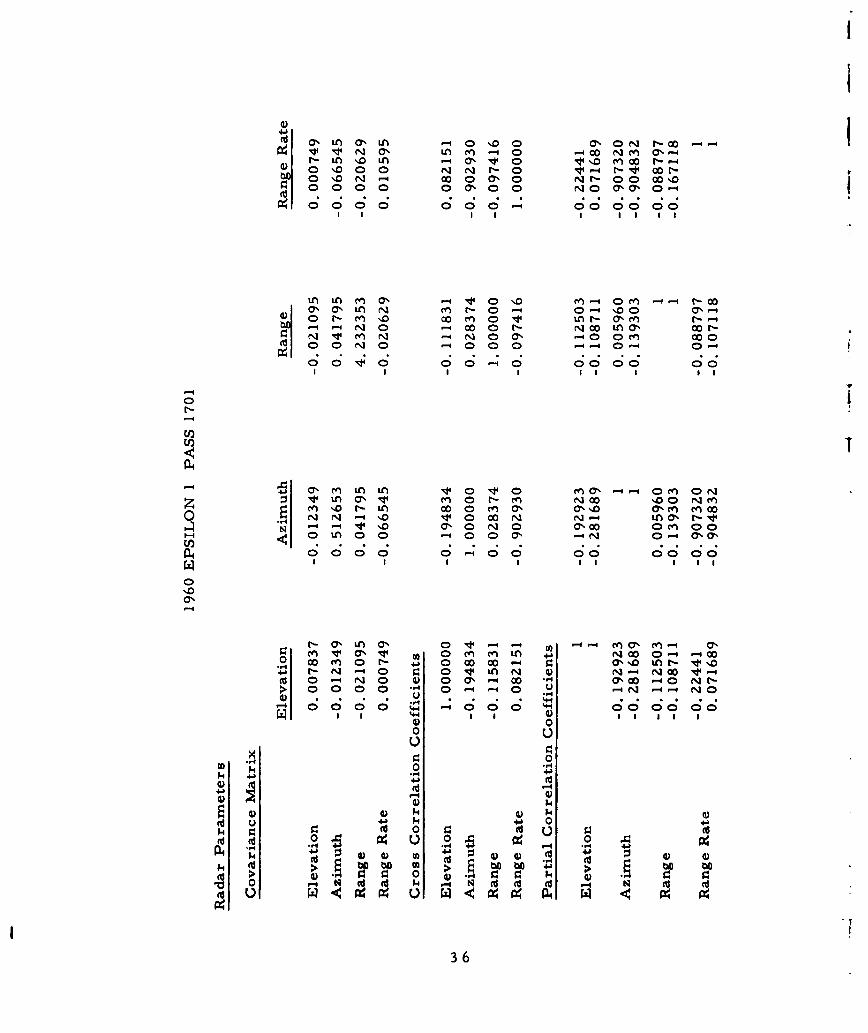
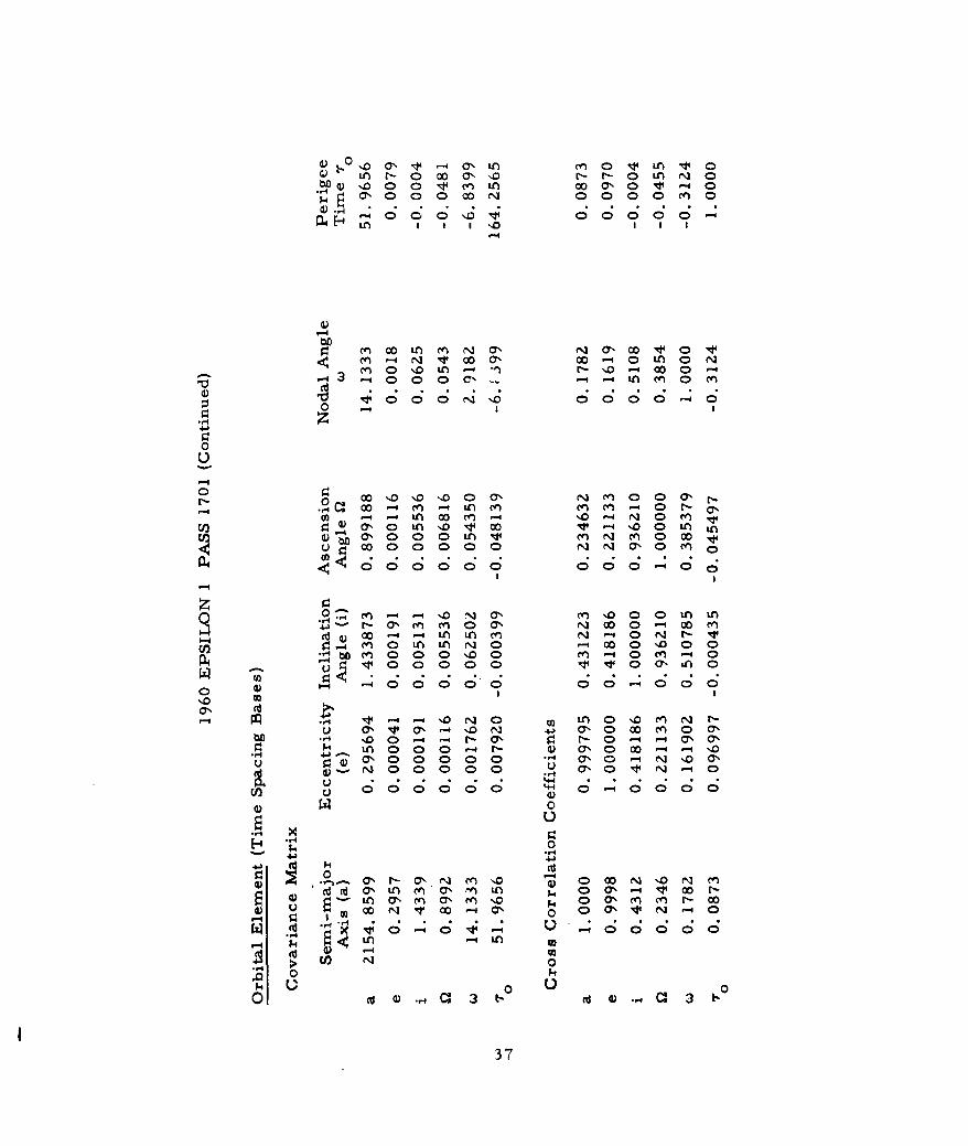
The partial correlation coefficients for the various time spacings
appeared to be relatively stable and show good agreement with the
simple cross correlation for both the radar parameters and the orbital
elements. The double sets of values shown for 1960 Epsilon 1 are due
to the correlation between two parameters, with one of the other two
parameters fixed.
35
a inaL u) O0 .0 a oN r'- 00-4 -
v v0 yO m o00 N n 0% 4 -4'0' L 0N Ln-0 0 %00 Mt00 co..
0 %0N 000 cl 000r 00 009; ; C; C; 9; 9; C; C; I ; C;
Lfn Un m q 1 0 ID fn -4 0 e -4 -4 00ca, c LnN M r- -4 0-~ %00 0-
o w m 0O14 V) r- a,( --
00 o 00-0 r ml0000) Y 00 r
-: N'r m~ r N4 4 r- o a 0 0Mco N
-4 a, m L n' Lo r 0 0'-r Nn ' 0 N )
0 N N 0 w' N N -4 LnO CY -'t
0 L O 0 -0 0 C7, -4N 0-4 a, c7
0 v0% 0mN00 0-00 004 00
C'1 N -0 0 0IV LAN 4) N - N~ 00 V(d 0- NO0 4) 0 0 '% M ,1()0-40 N r-
4) 00 ur"
0 -0
-14
CU u 4 $44 04b$ U 0 (d U 0 d
0 .4 -(d ®r4 U) m 4 )4 r 4 4
>U 0) . V 0 0 a4 9 4
36
'ODC 1-~ O\L U) 0 4 LA v 0' in) N o C'~ N N7 -o LA N O0
bb 0 0 0 v cN 000 0
.,44
P f E L ON N 0" N 0 " 0 0 1
1 - 0 0 04c c C ' -; - L C C
00
00N '00 .00 C 00z
C: (n 4 LA cn en m '0 NO a%
(02 ao LA 'o0 v 1~00 LA t LA4 0 0 LA vt cn Nl CA 0 001
u o 0 0 000a N Nl (710 c 0
P4 C; 00 00 0 0 0-0 0 c C
z0 CA -4nO %" CA.0 0 LA LA
41 N- 'cy A CA 0 0" N 00 0 -100 V-d op r- - LA LA cn N - O N N- V
M1 0 CALO LA NO - 00 0 100 0be (.1CA 0 0 0 '.00 -4 0 CA -0
P, C) 0 o~ 0 o'-Lo 0
V -4~ 0-4'.N 0 O 0 IDm 'ba .0 0 -4 - N )- O -4 -q P.
16 L oO 0 - N 0. -4 .4'D+.4a'r.oo 0 000 ONo-N00
NO 0 0 0 C; 00 C; N ; -0'4)
043 +1
+3d
a% r- aAC N cn LA a 00'. N~ N
~Lna% m 0% m %0 0 O0CY% m N-v N It 00 o. 0 " N - 0
LA 1L 0 0 0 0
., -4 N
0~4 ~ 00
0 c 4.-C31 -4 4.. C: 31
37
SECTION 3
CONC LUSIONS
This study has shown that the differential correction smoothing pro-
cedure is a solution of the generalized least square problem (Ref. 2).
The residuals obtained by fitting the observation with polynomial plus
an autoregressive scheme (Ref. 10) are uncorrelated and the standard
deviations of the radar parameters with the autoregressive scheme are
less than those obtained with polynomial fitting alone.
In the process of analyzing the behavior of the orbital elements it was
noted that the coefficient of skewness exhibits a degree of consistency
for different satellites and sensors. Furthermore it has been possible
to derive the variance of any orbital elements, as functions of the vari-
ance of the observations, the time of observation and description of the
motion of the satellite. It has been shown that the variance of any
orbital element is a minimum if the sum of the variances of the obser-
vations at a given time is a minimum for a specific computation pro-
cedure of the orbital element from observations. This indicates that
minimum variance orbital estimations are only relative minimums.
The behavior of the variance and skewness suggests that the computa-
tional procedure introduced a bias. The latter, in particular, cannot
be traced to a round-off error.
The problem of getting accurate position prediction of artificial satel-
lites is one of interplay between the quality of observations and the
analytical description of the motion of the satellite. How to trade these
factors depends upon the time allowed for deriving the orbit from obser-
vations.
38
The analytical expression showing this interplay has been derived and
represents the natural starting point for (1) an accurate prediction
scheme and (2) updating or intermixing criteria.
39
REFERENCES
I. "Contributions to Astrodynamics," Aeronutronic Publication
U-880, 1 June 1960.
2. Grossberg, M. , "The Linear Error Analysis of a Differential
Correction Procedure' RCA Report CR-588-71-SI, November
1961. (ESD-TDR-62-39)
3. Kochi, K.C., and R.M. Staley, Autonetics, "Methods for Analysis
of Satellite Trajectories," WADC Technical Report 60-214 (AD
247104), September 1960.
4. Bodwell, C., "Least Squares Smoothing by Orthogonal Polynomials
and Analysis of Variance',' Holloman Air Force Base, Report No.
MTHT 293.
5. Lassovszky, K., "On the Accuracy of Measurements Made Upon
Films Photographed by Baker-Nunn Satellite Tracking Cameras,
SAO Report No. 74.
6. Heinze, K. G,, "The Baker-Nunn Satellite-Tracking Camera:'
Sky and Telescope, Volume XVI, No. 3, January 1957.
7. Fitzpatrick, P.M., and G. B. Findley, "The Tracking Operation
at the National Space Surveillance Control Center ( NSSCC),"
2 September 1960.
8. Burington and May, "Handbook of Probability and Statistics with
Tables:' Handbook Publishers, Inc., 1958.
40
9. David, F. N., "Tables of the Ordinates and Probability Integral
of the Destribution of the Correlation Coefficient in Small Samples"
Biometrika, 1938.
10. Arcese, A., "A Time Series Analysis of Radar Observations on
Satellites'' RCA Report CR-588-77-S3, March 1962. (ESD-TDR-
62-40)
11. Tukey, J. W. , "Propagation of Errors, Fluctuation & Tolerances,"
Princeton University Technical Report No. 10, Contract No.
DA36-034-ORD-2297.
41
SYMBOLS USED f
p(t1 ) Range at time t.
A(t i ) Azimuth at time t.1
E(t i ) Elevation at time t.1 1
Site latitude
XSite longitude
i Time
(x, y, z) A geocentric coordinate represented vector
(x, y, z) in topocentric coordinates
r( t i ) A vector from earth's center to a point on orbit (at t.)
R Earth's radius
T2 Time increments
i( t i ) Rate of change of r(t.)
d i , Gi , H. Defined in text, functions of
s2 Defined in text5
P Defined in text
U, V, W Defined in text (vectors)
a Semi-latus rectum of orbit
e Eccentricity of orbit
v True anomaly of orbit
a A vector, defined in text
w The angle of perigee
N, M Vectors defined in text
G Gravitational constant
42
E Eccentric anomaly of orbit
T A constant of the orbit
0The angle of the ascending node
I The inclination of the orbit
I,J,K Unit vectors, defined in text
E(x) Tho expectation of X
i4 The "ith" moment of P about its mean, i=2, 3, 4P4The mean of PP
a E( x-x) (y-y)xy
'xyz E( x-x)(-Y)(-z)/x y zFxyzw Elx-x)(y-y) (z-z)(w -w) /axayaza
A, B Matrices, .,x3
a.. An element of A B
cxy E(x-x)(y-Y)
cxyz E(x-x)(y-Y)(z-Z)
C x E( x--)( y-Y) (z - )(w -- )
43
APPENDIX A
POLAR VERSUS CARTESIAN SMOOTHING
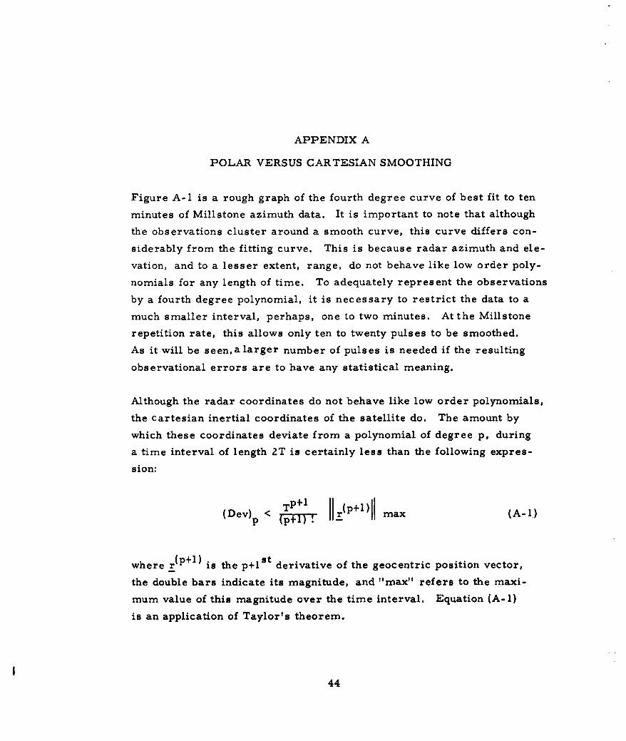
Figure A-I is a rough graph of the fourth degree curve of best fit to ten
minutes of Millstone azimuth data. It is important to note that although
the observations cluster around a smooth curve, this curve differs con-
siderably from the fitting curve. This is because radar azimuth and ele-
vation, and to a lesser extent, range, do not behave like low order poly-
nomials for any length of time. To adequately represent the observations
by a fourth degree polynomial, it is necessary to restrict the data to a
much smaller interval, perhaps, one to two minutes. At the Millstone
repetition rate, this allows only ten to twenty pulses to be smoothed.
As it will be seen, a larger number of pulses is needed if the resulting
observational errors are to have any statistical meaning.
Although the radar coordinates do not behave like low order polynomials,
the cartesian inertial coordinates of the satellite do. The amount by
which these coordinates deviate from a polynomial of degree p, during
a time interval of length 2T is certainly less than the following expres-
sion:
(Dev) < VTrl(P+l)m
where r( p I ) is the p+l s t derivative of the geocentric position vector,
the double bars indicate its magnitude, and "max" refers to the maxi-
mum value of this magnitude over the time interval. Equation (A-I)
is an application of Taylor's theorem.
44
Page 45
Azimuth
2700
1800
g00
10 m
Figure A-1. Millstone azimuth observations (dashes) andbest fitting fourth degree polynomial (curve)
I
by noting that (1) these quantities may be calculated without signi-
ficant error assuming a Keplerian ellipse, and (2) on this ellipse the
derivatives are maximized at perigee. The region of a-e space indicated
in the third column includes most reasonable and stable satellite orbits.
All formulas and numbers are in canonical units.
Table A-i
Magnitude of first few position derivatives is evaluated at perigee and
numerical bounds on these magnitudes.
r(p max over
a(l-e) > 1.05, e < 0.5
0 r a(l-e) cc
1 A r -0.5 1.2
2 r 0.9
3 +e r 51.0
4 (1+3e) r I2.0
5 \/I+c 1+9e) r -6.5 4.8
2 -8.
6 1+24e427e 2 ) r - 13.0
46
The second or third column of Table A-1 may be used with Equation(A-i)
depending upon whether the orbital elements are approximately
known. Combining the third column with Equation (A-1), Table A-2
may be obtained. Table A-2 expresses the maximum values of the in-th
tervals over which the inertial coordinates deviate from a p degree
polynomial by the given amounts.
Table A-2
2T versus p and (Dev)p
71P (Dev)p <1.1km (Dev)p < 0.1 km (Dev)p< 0.01 km
0 0.205 sec 0.0205 sec 0. 00205 sec
1 29.9 sec 9.56 sec 2.99 sec
2 157.00 sec 72.90 sec 33.8 sec
3 334.00 sec 188.00 sec 106.00 sec
4 529.00 sec 334.00 sec 210.00 sec
5 726.00 sec 499.00 sec 337.00 sec
Table A-2 shows that, if a 0.1-km deviation in the fit can be accepted, a
fourth degree polynomial may be applied to 5-1/2 minutes of data.
Thus, the following procedure has been developed for the orbit removal
from Millstone radar.
(1) From each pass, select the middle seven minutes of data
(Dev 4 (7 min) < 0.35 km).
(2) Transform the ranges, azimuths, and elevations selected in
Step (1) to cartesian inertial coordinates by the well-known
transformatio,,.
47
(3) Solve the three sets of likelihood equations for the selected
records of x, y, z.
(4) Use the solutions to the likelihood equations to evaluate the
fourth degree polynomials for x, y, z at all the tk points
selected in Step (1).
(5) Transform these polynomial points back to range, azimuth
and elevation and subtract them from the corresponding
observations.
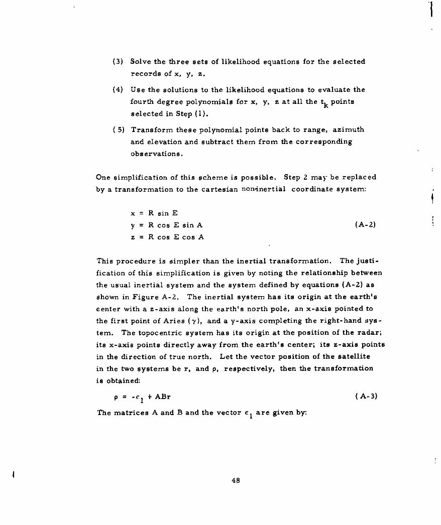
One simplification of this scheme is possible. Step 2 may be replaced
by a transformation to the cartesian non-inertial coordinate system:
x = R sin E
y = R cos E sin A (A-2)
z = R cos E cos A
This procedure is simpler than the inertial transformation. The justi-
fication of this simplification is given by noting the relationship between
the usual inertial system and the system defined by equations (A-2) as
shown in Figure A-2. The inertial system has its origin at the earth's
center with a z-axis along the earth's north pole, an x-axis pointed to
the first point of Aries (7), and a y-axis completing the right-hand sys-
tem. The topocentric system has its origin at the position of the radar;
its x-axis points directly away from the earth's center; its z-axis points
in the direction of true north. Let the vector position of the satellite
in the two systems be r, and p, respectively, then the transformation
is obtained:
P = - r + ABr (A-3)
The matrices A and B and the vector e: are given by:
48
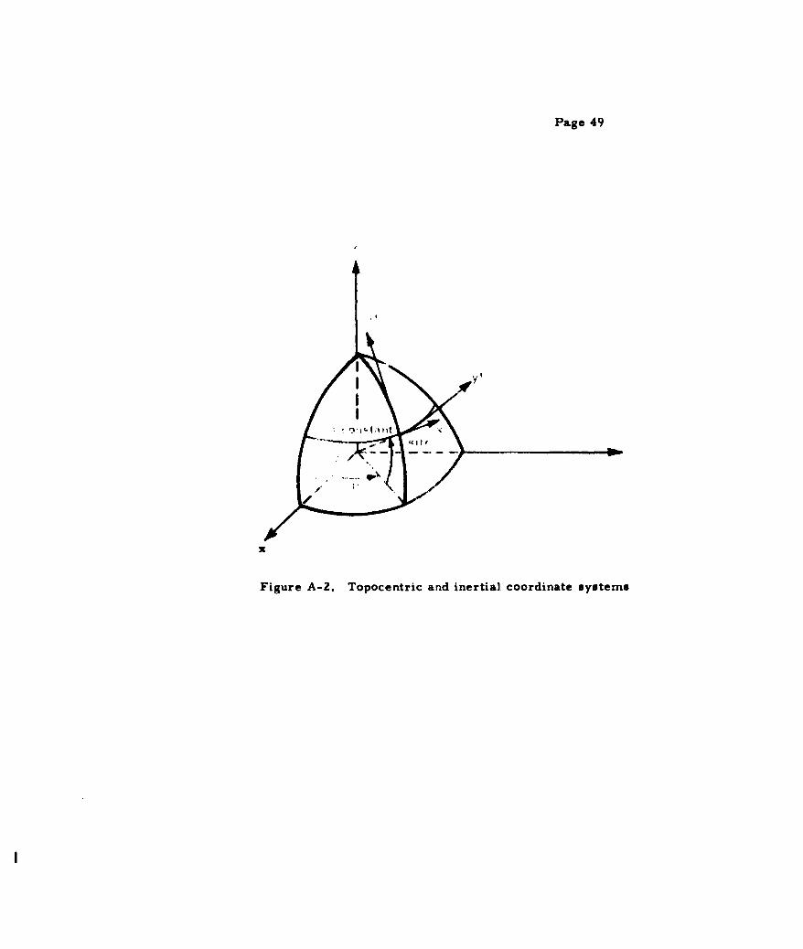
Page 49
IY
Figure A-2. Topocentric and inertial. coordinate systems
A1 cosa 0 sina) "s sin0. A .-.,oo 0 _,c Bsn CS0 1 0 0
(A-4)
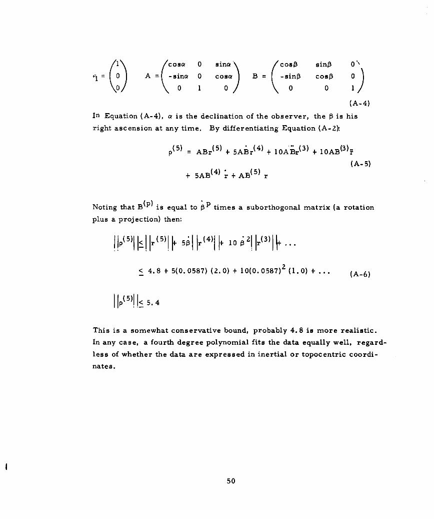
In Equation (A-4), a is the declination of the observer, the P is his
right ascension at any time. By differentiating Equation (A-2):
(5) (5) (4) + (3) + 10AB(3)
p =ABr~ 5 + 5ABr~4 + 10Ar 3 +OA 3 ~
(A-5)
+ 5AB ( 4 ) r + AB (5 ) r
Noting that B is equal to P times a suborthogonal matrix (a rotation
plus a projection) then:
li 511 Ir(5)1 501 Ir (4)1 10 0 - J()
< 4.8 + 5(0. 0587) (2.0) + 10(0. 0587)? (1. 0) + . (A-6)
This is a somewhat conservative bound, probably 4.8 is more realistic.
In any case, a fourth degree polynomial fits the data equally well, regard-
less of whether the data are expressed in inertial or topocentric coordi-
nates.
50
APPENDIX B
DISTORTION OF THE ERRORS
Since the polynomial coefficients estimated from a record are random
variables, the calculated values of the polynomials at each tk are also
random variables. If these values have standard deviations as large
as the deviations of the observations, the actual observational errors
will be masked. The deviations of the calculated values are calculated
here under two assumptions:
(1) at 2 6 That is, the data have no serial() x( tn) x(tj) '2 C x jk*
correlation, and the same coordinate observed at different
times has the same variance.
(2) tk+1 = t k + -'. That is, the observations are equally spaced
in time.
Assumption (1) is not valid, for even if it were true of range, azimuth,
and elevation, it would not be true that the cartesian coordinates would
have constant variances. Assumption (2) is approximately satisfied
for any radar - in particular for Millstone, r" = 6 secondE.
Given assumption (1), Equation (B-1) for the covariance matrix of the
coefficients is valid (with aR replaced by ax,, a y or z Given assump-
tion (2), the sums in the matrix may be calculated in closed form, and
the matrix analytically inverted. The results of this inversion are
shown in Table B-i. The left-hand column is the degree of the polyno-
mial. The matrix on the right hand has a A t row and
thcolumn. The quantity T, as defined previously, in one-half the time
51
jt oun h uniyT sdfne rvosyIi n-aftetm
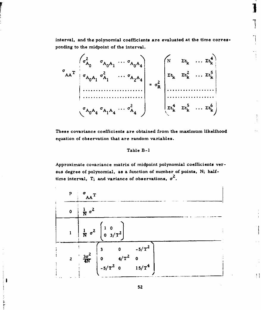
)I
interval, and the polynomial coefficients are evaluated at the time corres-
ponding to the midpoint of the interval.
(2 4>(aA0 a A A N Etk Etk
A TAa ,.. 2AA .t. 2 5AA A A Ek tk ZkI
0 1 1 2A4
a aa2 4 5 .. 6KA0 A4 AIA4 • 4 \E
These covariance coefficients are obtained from the maximum likelihood
equation of observation that are random variables.
Table B-1
Approximate covariance matrix of midpoint polynomial coefficients ver-
sus degree of polynomial, as a function of number of points, N; half-
time interval, T; and variance of observations, a
P aAA
012
1 0
3 0 -5/T 2
- 0 4/T 0
2 -yq02 4-5/T 0 5/T
52
I.
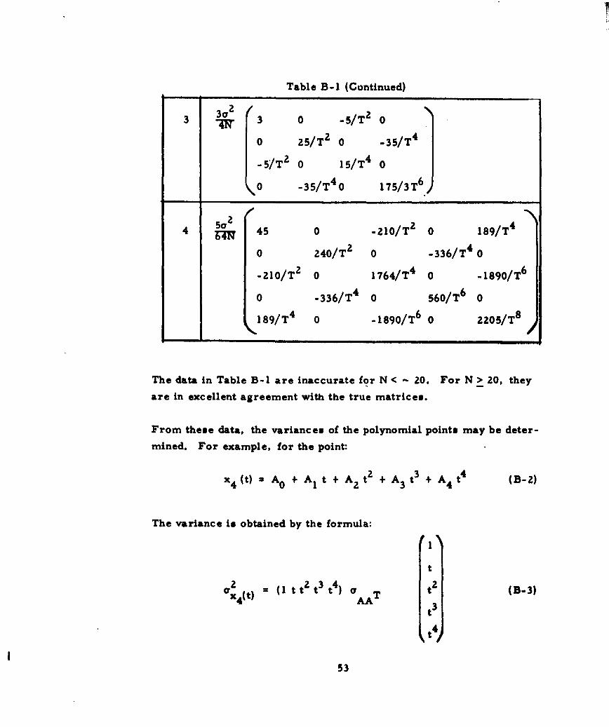
Table B-1 (Continued)
3 3 0 -S/T 2 0
o 25/T 2 0 -35/T 4
-S/T 2 0 15/T 4 0
0 -35/T4 0 175/3T 6
502
4 45 0 -210/T 2 0 189/T 4
0 240/T 2 0 -336/T 4 0
-210/T 2 0 1764/T 4 0 -1890/T 6
0 -336/T 4 0 560/T 6 0
189/T 4 0 - 1890/T 6 0 2205/T 8
The data in Table B-I are inaccurate for N < - 20. For N> 20, they
are in excellent agreement with the true matrices.
From theme data, the variances of the polynomial points may be deter-
mined. For example, for the point:
x 4 (t) = A0 + A I t + A2 t 2 + A3 t 3 + A 4 t4 (B-2)
The variance is obtained by the formula:
t
x4 (t) ( t 2 t3 t4 ) at 2 (B-3)x P) AA T3
t5
53
IT
as:
t - 2 t4 6-a 2 3 5 4,.o6 + 1
Fr 4(t) IT + 171.95 (15)8
For polynomials of lower degree, expressions similar to Equation (B-4)
are found. These expressions are listed in Table B-2. In Figure B-1
the square roots of these expressions and the ratio of the corresponding
standard deviations are plotted for several degrees and several values
of N.
Table B-2
Ratio of variance of polynomial point to variance of observation,2 la for various degrees of polynomial, p, as a function of N
7x (t) xp
and of the ratio of time from midpoint to half interval, K = t/T.
2 ,2
I ~x P t x
0 a 2/N
1 ac2/N ( 1+3K 2 )
2 V2/N ( 2.25-4K2+ ..25K4 )
3 a 2 /N ( 2. 25+11. 25K2-41. 25K 4+43.75K 6)
4 a 2/N (3.516-14. 064K 2+1 14. 844K 4 -251. 562K 6+71. 953K 8 )
Figure B-I indicates that with N=70 and fourth degree smoothing, up to
80 percent of the computed points have a standard deviation less than
one-quarter of the observation deviation; furthermore, at the extreme
554
-I
Page 551. 5
N1.0
0.-N = 101.
0.7-12nd
o.- a N:=25 degrei 0. 5
0.4- N =50
0. 3 N= 100 -0.3
0.2Z
N 10{ .
1. 0 .
0.9- N a2Z 3rd0.7-____________ degreo
06- a________ N =50 0.5
0. 3
0. 2-
1.0
0.8- 4th0.7-N z 50 degre4o.6-N:= 70
0. 5- IOOJ0. 5
0. 3-- Ox0. 3
Ku t/T
0 0.1 0.2 0.3 0.4 0. 5 0.6 0.7 0.8 0.9 1.0
Figure B- 1. Ratio of standard deviation of estimated polynomialpoint to standard deviation of observations, versusratio of time from midpoint to half interval, forsecond, third, and fourth degree smoothing.
edges of the observation interval, this ratio is about three-fifths. How-
ever, since assumption (1) of the previous section - that the observa-
tion deviations in each coordinate are constant - is not true, the ratio
may be somewhat higher than this value. For this reason, it is con-
sidered advisable to chop off the errors at about 80 percent of the way
to the edges.
A smoothing procedure has thus been established to be applied to Mill-
stone data covering seven or more minutest
(1) Select the middle seven minutes of data.
(2) Transform range, azimuth and elevation to cartesian coordi-
nates by Equations (A-2).
(3) Find the coefficients of the fourth degree polynomials of closest
fit to the three records obtained in Step (2) by solving the likeli-
hood equations assuming observations are random variables.
(4) Evaluate the three polynomials found in Step (3) at each of the
71 time points selected in Step (1).
(5) Transform the polynomial points found in Step (4) to ranges,
azimuths and elevations by inverting Equations (A-2) and sub-
tract these values from the observed values of range, azimuth,
and elevation.
(6) Discard the first and last seven sets of differencesleaving 57
"range errors," 57 "azimuth errors, and 57 "elevation
errors,"
This procedure has been devised for Millstone data, which are availa-
ble at 6-.second intervals, and which have standard deviations of about
one to two kilometers. For different radars, a different procedure is
necessary, but the formulas, tables, and graphs presented here should
be sufficient to derive such a procedure. J
56 *1
APPENDIX C
CONFIDENCE BOUNDS FOR SAMPLE CORRELATIONCOEFFICIENTS AS A TEST FOR RANDOMNESS
In order to determine a test of randomness for a set of samples, an
initial hypothesis p = 0 is taken. On the basis of the serial correla-
tions of the sample, a procedure for testing randomness by employing
the distribution function of the correlation coefficients is established.
A 90-percent confidence curve on the correlation coefficient is shown in
Figure C-1.
Given a sample of size m, it is desired to test the sample for random-
ness. One approach to this problem rests upon an examination of the
serial correlations. The serial correlation coefficient is given by
coy (x., X
rk= cv (x x k=0, 1, 2... (C-1)[var x , var x3+k]
If the elements x, x j+k are separated into two groups, then the ele-
ments x. and xj+k can be considered as elements from separate sam-
ples, both samples being of the same size, n.
It: is now assumed that the population has a bivariate normal distribu-
tion. That is, the samples xj and xj+k can be considered as coming
from a bivariate normal population. The distribution function of r as
given in Ref. 8 is:
57
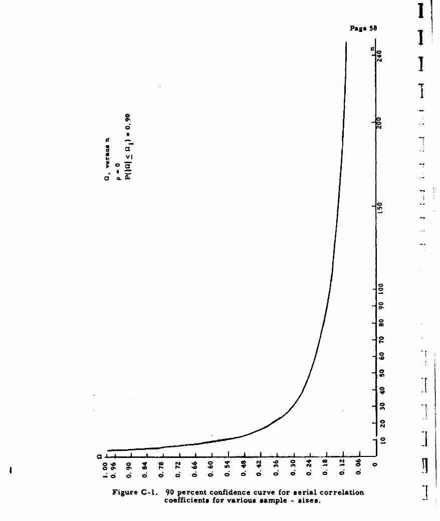
Page 58
C1:
VII CD
r- rn
IIn
Figure C-1. 90 percent confidence curve for serial correlation "
coefficients for various sample - sizes,.-
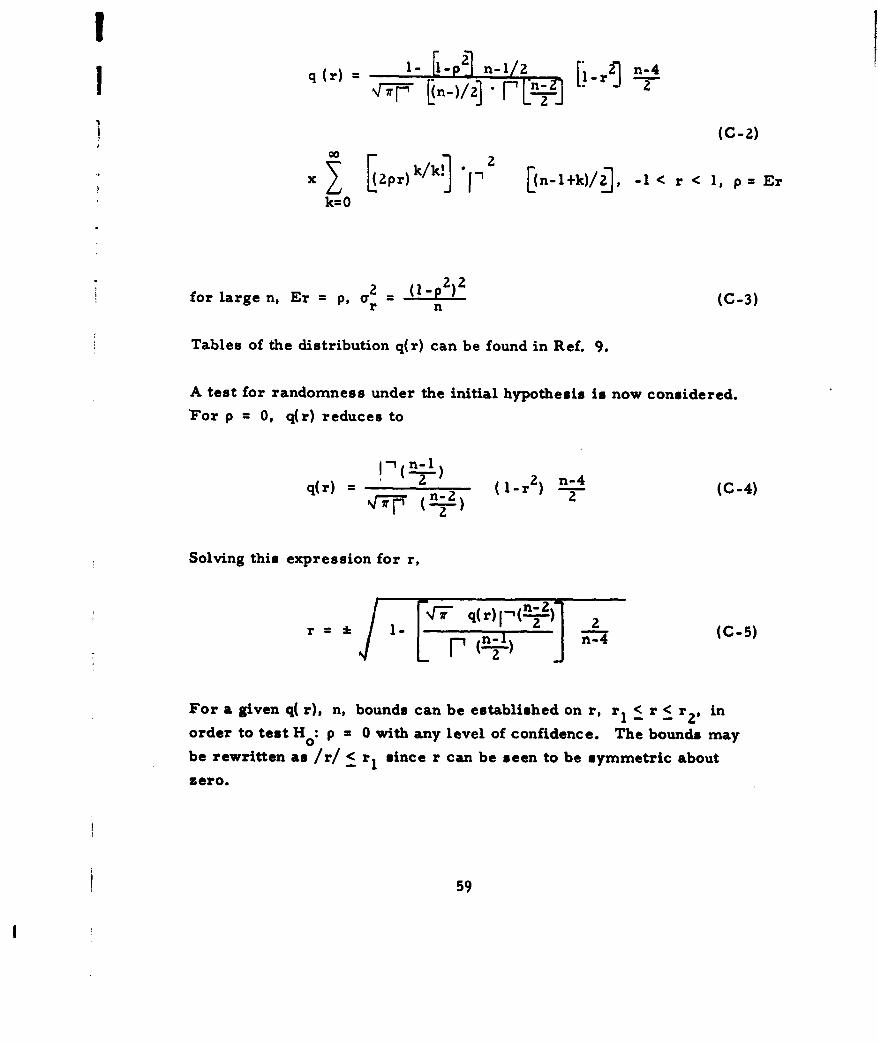
1q"r)>= 1- [i "] --,! [j.r,] ,,-q (n-/2 2.4~
(C-z)
x j2pr)'] ' [(n-I+k)/ , -1 < r < 1, p = Er
k=0
2 (I-p 2 )2
for large n, Er = p, ar n (C-3)
Tables of the distribution q(r) can be found in Ref. 9.
A test for randomness under the initial hypothesis is now considered.
For p = 0, q(r) reduces to
n-i (n- l
q(r) 2 r (!.r2) n-4 (C-4)
Solving this expression for r,
r = /i. [q7 q(r)[-Ij-)] (C5
For a given q( r), n, bounds can be established on r, r1 < r < r2 , in
order to test H0: p = 0 with any level of confidence. The bounds may
be rewritten as /r/< r1 since r can be seen to be symmetric about
zero,
59
To use the tables in Ref. 9, values of p and n are needed. For a given
probability, a value of r can be determined. One such set of values is _
included in this report. These values are for a Two-Tailed Test of H 0
p = 0 with a probability of 0.90. The curve which follows the table is
merely a graphical representation of the results with only the upper
curve recorded since symmetry exists about zero.
For each serial correlation coefficient, the number of pairs of observa-
tions is plotted against r on the graph. If IrI falls under the curve, it
may be saidthat the sample is random with a probability of 0.90.
60
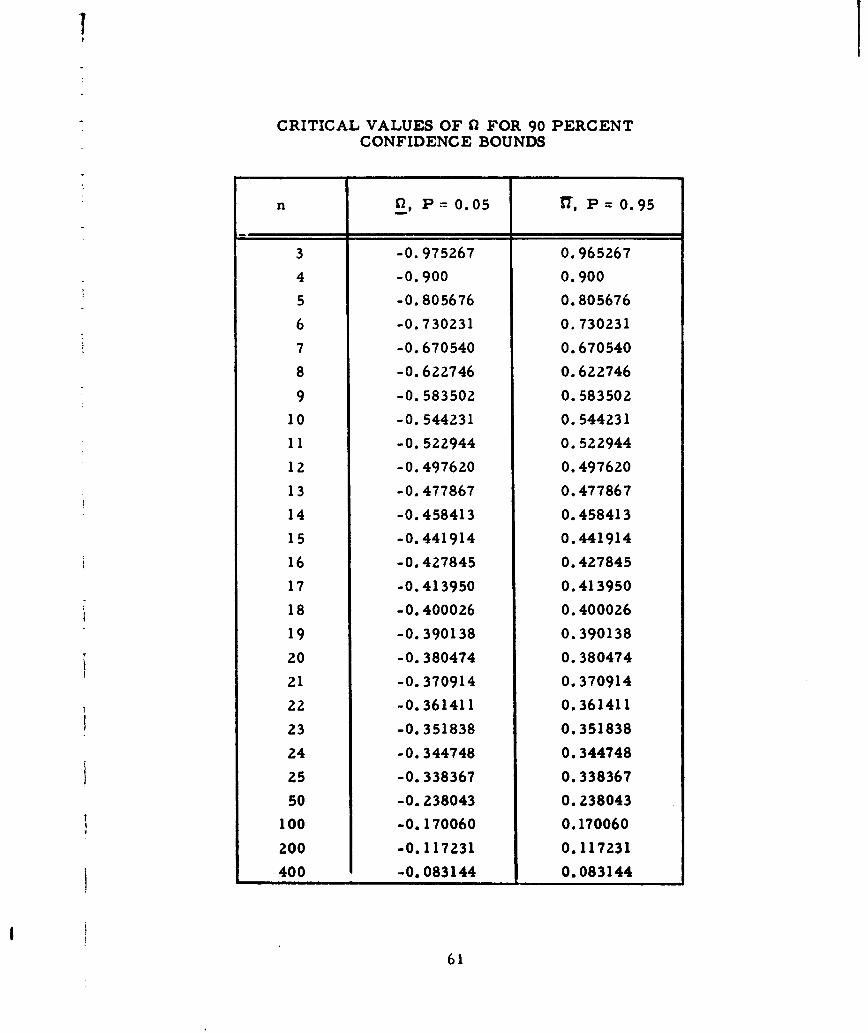
!I
CRITICAL VALUES OF 0 FOR 90 PERCENTCONFIDENCE BOUNDS
n C, P = 0.05 17, P = 0.95
3 -0.975267 0.965267
4 -0.900 0.9005 -0.805676 0.805676
6 -0.730231 0.7302317 -0.670540 0.670540
8 -0.622746 0.622746
9 -0.583502 0.583502
10 -0.544231 0.544231
11 -0.522944 0.522944
12 -0.497620 0.497620
13 -0.477867 0.477867
14 -0.458413 0.458413
15 -0.441914 0.441914
16 -0.427845 0.427845
17 -0.413950 0.413950
18 -0.400026 0.400026
19 -0.390138 0.390138
20 -0.380474 0.380474
21 -0.370914 0.370914
22 -0.361411 0.361411
23 -0.351838 0.351838
24 -0.344748 0.344748
25 -0.338367 0.338367
50 -0.238043 0.238043
100 -0.170060 0.170060
200 -0.117231 0.117231
400 -0.083144 0.083144
61
I
APPENDIX D
DERIVATION OF THE ORBITAL ELEMENTS
This appendix summarizes the equations needed to obtain the orbital
elements from observation data. The Herrick-Gibbs method is used in
determining the position vector and velocity vector of an observed satel-
lite.
D. 1 DETERMINATION OF INERTIAL COORDINATES
In general, the observations of a satellite are made with reference to a
given site of known latitude and longitude. To derive the orbit of this
satellite the observed positions of the satellites are referred to as a
geocentric inertial reference.
Let the earth's center be the origin of the geocentric inertial reference.
The axis of the earth represents one of the axis, Z, of the reference.
One of the axes. X, is in the equatorial plane and directed toward the
first point in Aries or vernal equinox; the other, Y, is also in the equa-
torial plane and orthogonal to X. Let X', Y', Z' denote a topocentric
reference system whose origin is the site. The X1 axis coincides with
the vertical through the site, Z' is the horizontal plane about the site and
directed toward the north, and Y' forms an orthogonal system.
Let 0 be the angular rate of the earth's rotation in radians per second
and let the earth be spherical of radius R. If X', Y', Z' is a point in
the topocentric reference and X, Y, Z is a point in the inertial reference
then:
621
*1
i
Cos X i X05co 0 -sin e x
= sin X cos X 0 0 1 0 Y1O 0 0 sin o cos zi
where 0 is the site latitude, X* is the site longitude and X* = X + b t.
If the observations of a satellite about the site S are range, p, elevation,
E, and azimuth, A,
x (iy psin E A
( y !t) p cos E sin A
P z' (t) p cos E cos
then the position of the satellite in the inertial coordinate is represented
by
(t I os X* -sin IX 0 cos 0 0 -sin (t )sinE(t )+R
r(t 1 ) Y(t = s X cos X 0 (0 1 0 p(t) cosE(t )sinA(t 1 )
(tl) 0 0 1 in 4 0 cos */\p(t1 )COsE(tl)cosA(tl)
where t I denotes the time of the observation
D. 2 DETERMINATION OF POSITION AND VELOCITY VECTOR
From observations through vector positions,r (tI), r (t 2 ), r (t 3 ) are
determined using the transformations in subsection D. 1. These posi-
tions are determined at approximately equal intervals of time. With
these vectors r (t 2 ) andLr(t 2 ) are derived using the Herrick-Gibbs
method.
63
V
r(t 2 ) = r(t 2 )
"r(t 2 ) - -dr(t) +d rt ) +d 3 r(t 3 ) 7
where d =G + H (ti
and H= '2/12, H 2 = 2 - 71)/12, H3 = 1/12
GI , [r.1T2 i .2) -I. G_ (T2 _ . 2 ( .,r.+7.) I
G= 7 [,i 'a( 7 +72)] -1
where T I = t2 " tl and 'T2 t3 " t2
D. 3 DETERMINATION OF ORBITAL ELEMENTS
With the values of r (t 2 ) and "r (t 2 ) the orbital elements are determined
as follows:
2 -
r r r
5 r* rU
r = r • rr
SU = rlrI -
r r-r r
- r 2 (i 2 - i Z
w! xv[4 !I
64 H]Ii
!11 1 2 .2
e2 r2 ;2 2)
2 r ( -
sin v _ rs
e cos v -
v tan-1 [ e sin vi
= U e cos v- V e sinJ
Uz e cos v- Vz e sinv
a =(- a WY + a Wx)/ W2T
ayn = ( -a x WxWZ - ay W W z a z
= tan-, u -- w + v
65
I
U cos u - V sin ux x "
N= U cos u - V sin u- y y
U cos u - V sin u
- U sin u + V cos ux x
M= U sin u + V cos uy x
U sinu + V cos uz z
sin (V-E) 2 rG (e sin v) (e co + e in v
r I-(e sin vcos(v-E) = 2 -- K 7 +ecoov"r r Z 1 ez
.,-(,, ,-i
v-I = tan" 1 Csin (v-'E)
• sin E r (t- T) E- e sinE
T= (E - e sin E) +t 2
6r
66 -1
I = tan-1 (1, 0, 0)
IF
I =tan - ] K =(0, 0,1)
Thus the six orbital elements are defined, namely
- [a, e, i, wt (?, TI
I6
I
APPENDIX E
THE MOMENTS OF PREDICTED POSITION ERRORFROM MOMENTS OF ORBITAL ELEMENT ERRORS
This appendix presents the method for obtaining the statistics of the
error in the predicted position of a satellite as a function of the statis-
tics of the error in orbital elements.
E. 1 CALCULATION OF INERTIAL GEOCENTRIC COORDINATESFROM ORBITAL PARAMETER-
E. 1. 1 STATEMENT OF THE PROBLEM
The determination of ephemeris of particular satellites from radar
data which are subject to various errors will give predicted parameters
subject to errors. The inputs are the orbital elements, which have as-
sumed moments and comoments. The geocentric and topocentric iner-
tial coordinates are then derived with their respective moment distribu-
tions. The initial orbital information was considered to be non-indepen-
dent data, and the analysis utilized the first four moments to derive
formulas for the corresponding moments of the geocentric inertial coor-
dinates. These formulas indicate the procedure for the computation
of such terms, but due to their length they were approximated to include
only powers of order < a2 as they appear in Equations E. 2. 12, E. 2. 13,
and E. 2. 14. The required partial differentials for substitution into
these equations were then derived. The geocentric inertial coordinates
are then transformed to topocentric coordinates and subsequently into
radar parameters. The process for the computation of these error
moments is an identical procedure as previously employed. The addi-
tional required partial differentials for the radar parameter computation
have also been evaluated.
68
-1
The calculation of the inertial geocentric coordinates from the orbital
elements assuming a Keplerian system, and no orbital errors are
outlined here. From the initial orbital elements (a, e, 0 T i
are geocentric inertial cartesian coordinates are derived. The "ox"
axis is assumed to point to the first point in Aries through the Greenwhich
meridian at time T o, the "oz" axis is through the north pole and "oy"
completes the right-handed system.
Assuming a Keplerian system the magnitude of the radius vector at any
given time T is given by
a (l-e Z(l.1)r= + e cos v
where v is the true anamoly which is related to the eccentric anamoly
and time by
Cos cos E-e E (1.2)cos v= -e coo E
and( - TO) = E - e sin E E (1.3)Ia
From Equation E. 1. 1 the geocentric inertial coordinates can be obtained
x = r (CoS aO cos (W0 +v) -sinQ 0 sin (w0 + v) coh i)
x=r (sin 0 coS(W +v)- cos a sin(W +v) cosi)
z= r (sin (wo+ v)sini)
E (1.4)
The ephemeris of the topocentric cartesian coordinates for a given
radar site at latitude # and logitude A 0 is given by
69
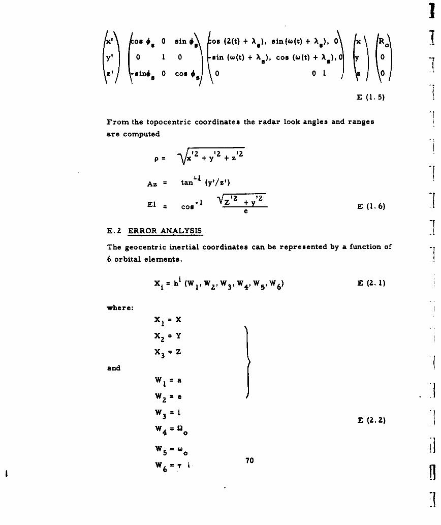
yi 0 1 0 n (w(t) + As), cos (W(t) + ),. O
sin# 0 cos 0 0 1 0
I~IIE (1. 5)
From the topocentric coordinates the radar look angles and ranges
are computed
P'2 '2 + '2p= +y 2+z
Az = tan (y'/z')
El = 1 VZ 42 'co +y E 0 .6)
E.2 ERROR ANALYSIS .
The geocentric inertial coordinates can be represented by a function of
6 orbital elements.
X h hi (W 2,W2 , W3 W4 ,W 5 ,W 6 ) E (2.1)
where:
x 1 =X
x 2 =Y
and
W =a
W2=
w 3 =i E (2. 2)
W4 0
W5 o
70
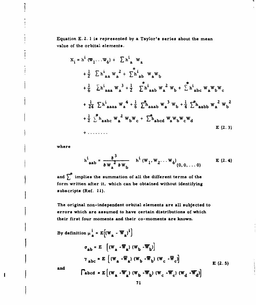
Equation E. 2. 1 is represented by a Taylor's series about the mean
value of the orbital elements.
xi I"6 ) + E.h h' W a
+I 'haa W 2 + h'b WWb
Sa aabWa abc c
I2+ Lh 1 W +1 Eh W Vw+ h' 2 2
+aa a 2 'aabca b 4 1-' abba b1 1 ~ 2
2 hab a WbW + Lhabd WaWbWcWd
E (2.3)
where
h - h h (WIW 2 .. W E (2.4)Wa Wb (0,O,...O)
and V implies the summation of all the different terms of the
form written after it, which can be obtained without identifying
subscripts (Ref. 11).
The original non-independent orbital elements are all subjected to
errors which are assumed to have certain distributions of which
their first four moments and their co-moments are known.
tI By definition a E[(Wa - Va)i]
a ab= E [(Wa -Wa) (Wb -Wrb)]
'Yabc E [(W a Wa) (Wb -Wb)(W c ]E (2. 5)
and rabc = [(a a )(Wb -Wb) (Wc W*)(Wd Wd)]rbd=[(Wa -Va c d
71
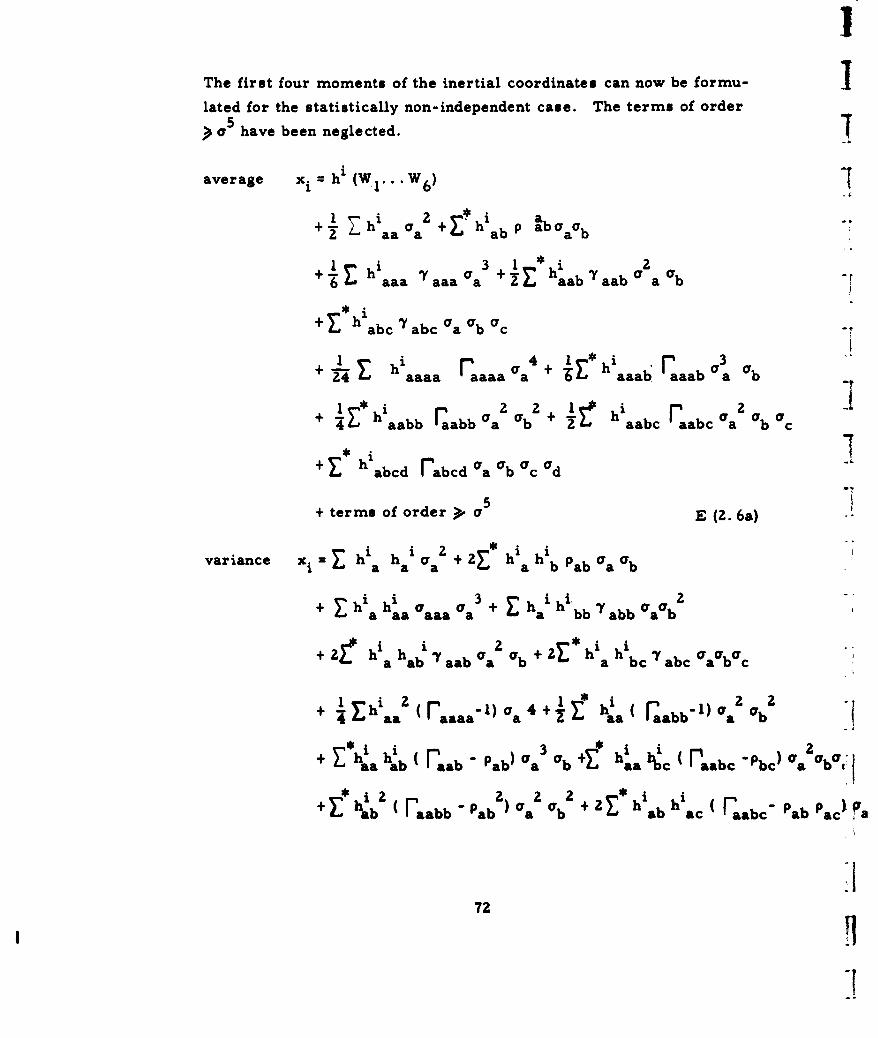
IThe first four moments of the inertial coordinates can now be formu- Ilated for the statistically non-independent case. The terms of order
a5 have been neglected.
average xi = hi (WI... W6 )
aa a + iab aaab
+ hi a b aaaaa aaaa a + aab "ab a
+ h abbla bc aaca b abcc
I hd r 4dva4-iancaaaaa aaa + - h a aa b r aaab a a ab
4h + aab a + h ab raab c a a c+ 4 baabb r a 2 b 2 a abc aa
+ !hi4* hi,
+ Zh~abcd rabcd Oraa b hb bd b
5 m
+ terms of order ,a E (2. 6a) -
+ h i h i a h 3 + EIaaa aaa a + al hbb 7abb ab
+ 2f hi h ia F 21 *h i h i
ab ab b a b + a bc 7abc abac
4 I haa - (raaaa-l , a4+ haa ( faabb-l) 'a Ob - -
N:ha ab Faab " Pab ) % %0' +E hia h c( raabc: "Pbc) ab , 4
+ hab ( raabb "Pab)a b + ab ac 'aab" Pab Pac' a
72
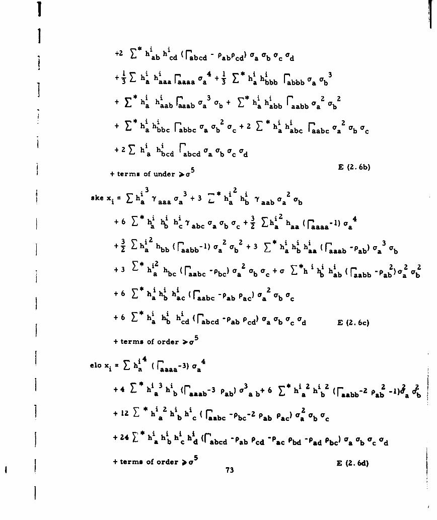
II+2 * h hd
ab cd (rab cd " PabPcd ) 'a 'b 'c 'd
+ .h' h' 4, ° + * h h * r" 33+.h ahla +.aaa 'a 'S a bb rabbb 'a 'b
ha aab ba 7b ha abb aabb "a b
i*j 2 ~'*i2+ h h ib abb °ab q +2 h ha h b b 0 b o
+ 2 hi hi F a a c
a bcd abcd
+ terms of under oa5 E (2.6b)
eke x. .h i3 0a3 .a2 .ha 2
= a 7aaa + 3 h hb 1 aab 7a ob
ha hc abc ab c+ haaa aaaa aa
+ 3 Z 2h2 2 +3Ei h *jjhi 03aa bb ( aabb-) Ora Gb + b ( aaab' Pab) ab
i2 2b I 1 2 23 ha hbc raabc-Pbc)aa b 7 +a h hhab (raabb Pab) a a a b
+6 h h - p c)G OGaCra ac (raabc "Pab ac
+6 . hi i hI h'
+6b cd (dabcd Pab Pcd) Oa b d6c)
+ terms of order >o5
elo x h1 i r -3) a*1X*£.a aaaa a
+4 3 3 hi 3 p 3 + 6 Zhia2 hi22a b (Faaab- ab) qa b6 a b (Iaabb "Z Pab a b] + 12 .*h i 2 hi hi ra'Pc 2 ac
a b c ( raabc Pbc 2 Pab P 0a b
a+4* h h hd (hIabcd " ab Pcd "ac Pbd Pad Pbd aa % 7c 'ad
J + terms of order ;oa"73 E (Z. 6d)
1
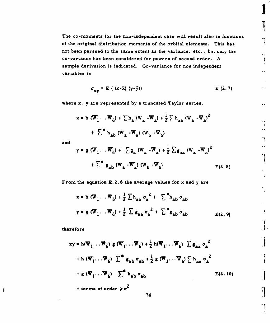
I
The co-moments for the non-independent case will result also in functions
of the original distribution moments of the orbital elements. This has
not been persued to the same extent as the variance, etc. , but only the
co-variance has been considered for powers of second order. A
sample derivation is indicated. Co-variance for non independent
variables is
Oxy = E ((x- ) (y- )) E(2.7)
where x, y are represented by a truncated Taylor series. .
x h (1...W 6 )+ Eh a (Wa -Wa)+ z.Zhaa (Wa -Wa)
+ E" hab (Wa -Wa) (Wb "Wb)
andy ff9 ('l"" W6 ) + E ga (W a " Wa ) + 'Egaa (W a "a ) "
+ gab (W a "Wa) (Wb "Wb) E(2. 8)
From the equation E. 2. 8 the average values for x and y are
x h (W..W 6 )+I haaOa 2 + *h aboab
Y; g (WI... w 6) +' aa aa + gab orab E(Z. 9)
therefore
xy = h('l ... V6) g (71I...W 6) + -Zh(W1. . . W6) gaa ra
+h (W1 ... W 6 ) Z* ga~b+ Wl"1~ha
+ h (71 ..W 6 9 b+1 *1**V6
+ g (Wh1 . VW6 ) h ab aab E(2. 10)
+ terms of order ;o 741
74r
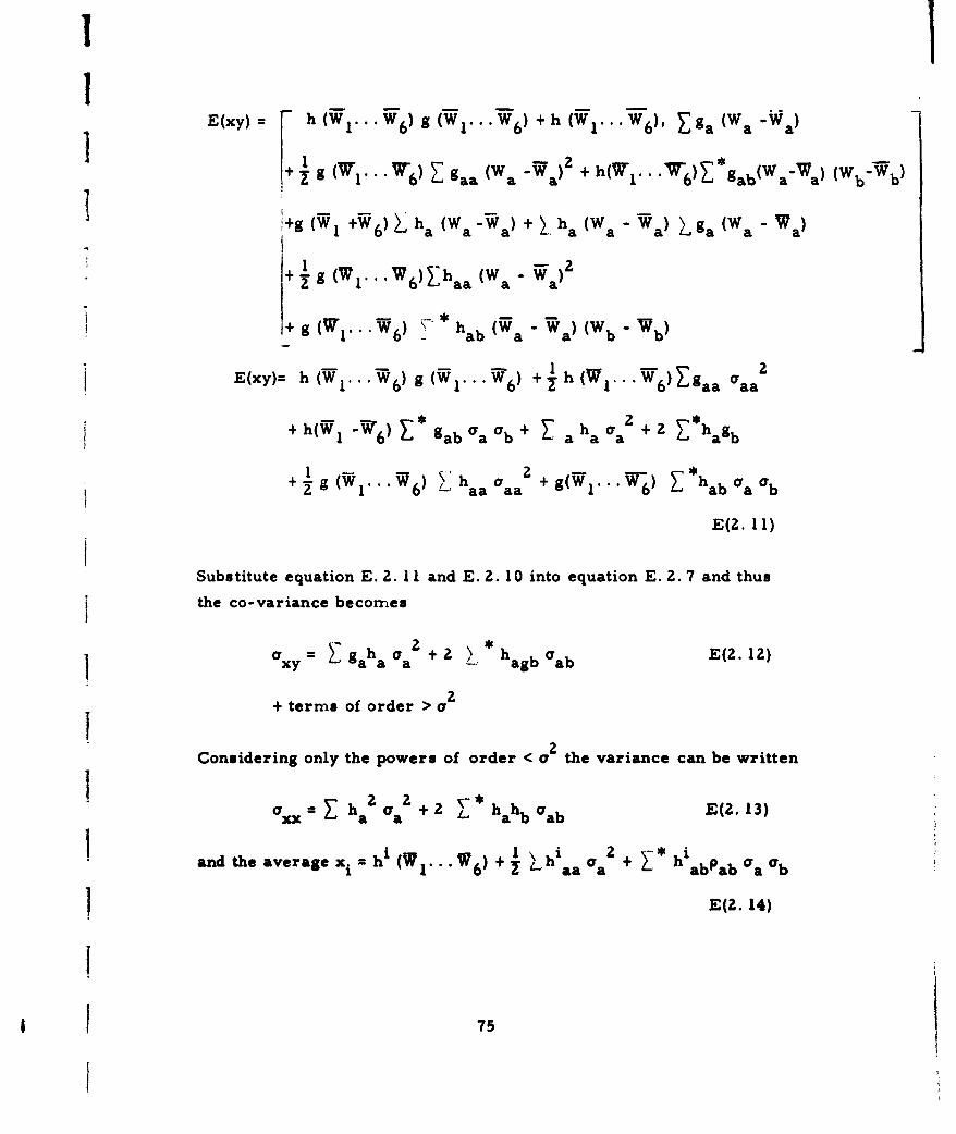
IIE(xy) - h ( 1 ... 6) g (W...W6 ) + h ( 1 ... W 6 ), g. (Wa a)
T+ I * ( "6) Z gaa (Wa -Wa) 2 + h .. "6)*gab(WaVa) (WbWb)
i+g (WI +W6) L ha (Wa -. ) + 1 ha (Wa "Wa) .ga (Wa Wa)
+ Ig (W ... W6)ZEhaa (Wa 2- Wa)
2 as,(W a 1i + g (1-...6) h hab (W a " r) (Wb " b
ab a b b.... 2
E(xy)= h (WI...W6) g (WI...W 6 ) + h (WI.. .W6)Zgaa aaa
+ h(Wh -26) gab Oa + a a +a 2 *hb
1 -6 aah a 2 +g(W 1 . .W) Z *h2" 1 6)' ' aa aa" ab 0a ab
E(2. 11)
Substitute equation E. 2. 11 and E. 2. 10 into equation E. 2.7 and thus
the co-variance becomes
a xy= Z aha a2 +2 * hagb crab E(2.12)
22I + terms of order > cr
Considering only the powers of order < c2 the variance can be written
xx= aha2 a +2 h* hahb ab E(2. 13)
and the average x. = h (W I W) + h * habab a b
E(2. 14)
75
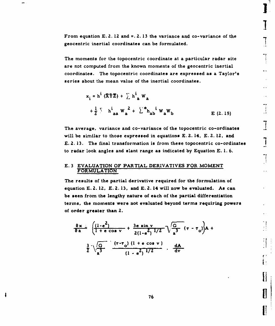
,
From equation E. 2. 12 and -2. 13 the variance and co-variance of the
geocentric inertial coordinates can be formulated.
"T
The moments for the topocentric coordinate at a particular radar site
are not computed from the known moments of the geocentric inertial
coordinates. The topocentric coordinates are expressed as a Taylor's
series about the mean value of the inertial coordinates.
- h ix=h i + ' h i Wxia a
+ hi W 2+ L*hi W W2 aa a aab ab E (2. 15)
The average, variance and co-variance of the topocentric co-ordinates
will be similar to those expressed in equations E. 2. 14, E. 2. 12, and
E. 2. 13. The final transformation is from these topocentric co-ordinates
to radar look angles and slant range as indicated by Equation E. 1. 6.
E. 3 EVALUATION OF PARTIAL DERIVATIVES FOR MOMENTFORMULATION
The results of the partial derivative required for the formulation of
equation E. 2. 12, E. 2. 13, and E. 2. 14 will now be evaluated. As can
be seen from the lengthy nature of each of the partial differentiation
terms, the moments were not evaluated beyond terms requiring powers
of order greater than 2.
aX (1-Co3e sin v "+!a + e con v 2(1e) 2/ )' "~ a 0o-
(,r-)1 + e cosv) dA
a ( -er) 1 / "
76I
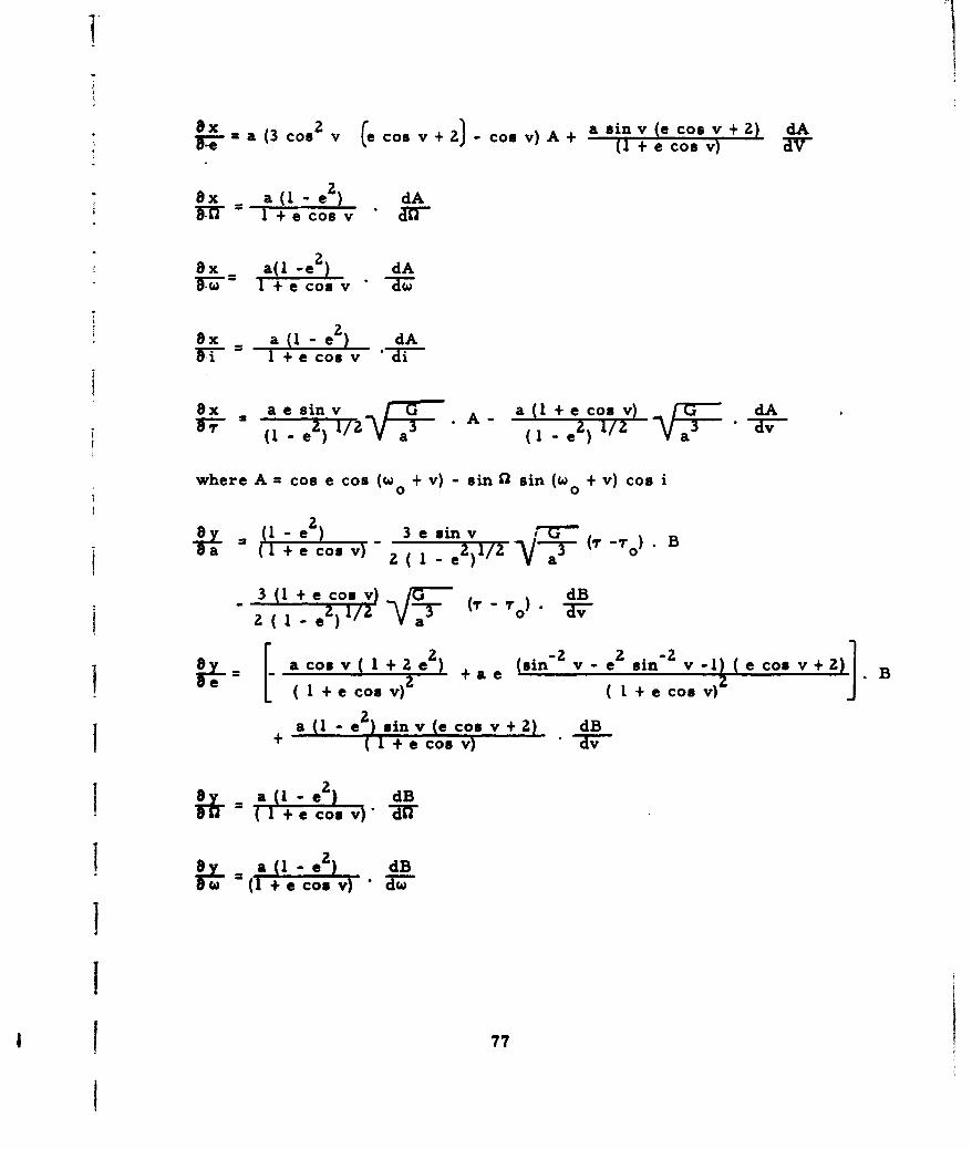
?A
exa 3 oo2 v (e coouv +4)coouv) A asinvie coomv+2) dA-a s(!+ecos v)
bx a(1 - e2 ) dAiK- = +ecoov -
ax a( -e2 dA- +e c-os v
ex a (I - e dAIF- = + e coo v "
-~ (I - Z eF 2. A-( 1/e2 Ti
where A = cos e cos (wo + v) - sin 91 sin (W + v) cos i0 0
a zeinS(I -e Z 3 e sin vi"a = (T + e cos v) 2 2 1/ 2 (,r --ro ) . B
3 (1 + e cosovr dBz 2(1- /e) 0/ r (,r- ro) ,
Fa conv - e 2 sinv2 ve 1) e cn BBI + c(v I + e oo v))
a(I e 2 inv(ecoov+2) dB
( I + +e cos v)" W
OF a Q1- e•2 dB+ ecoov) *"I
I
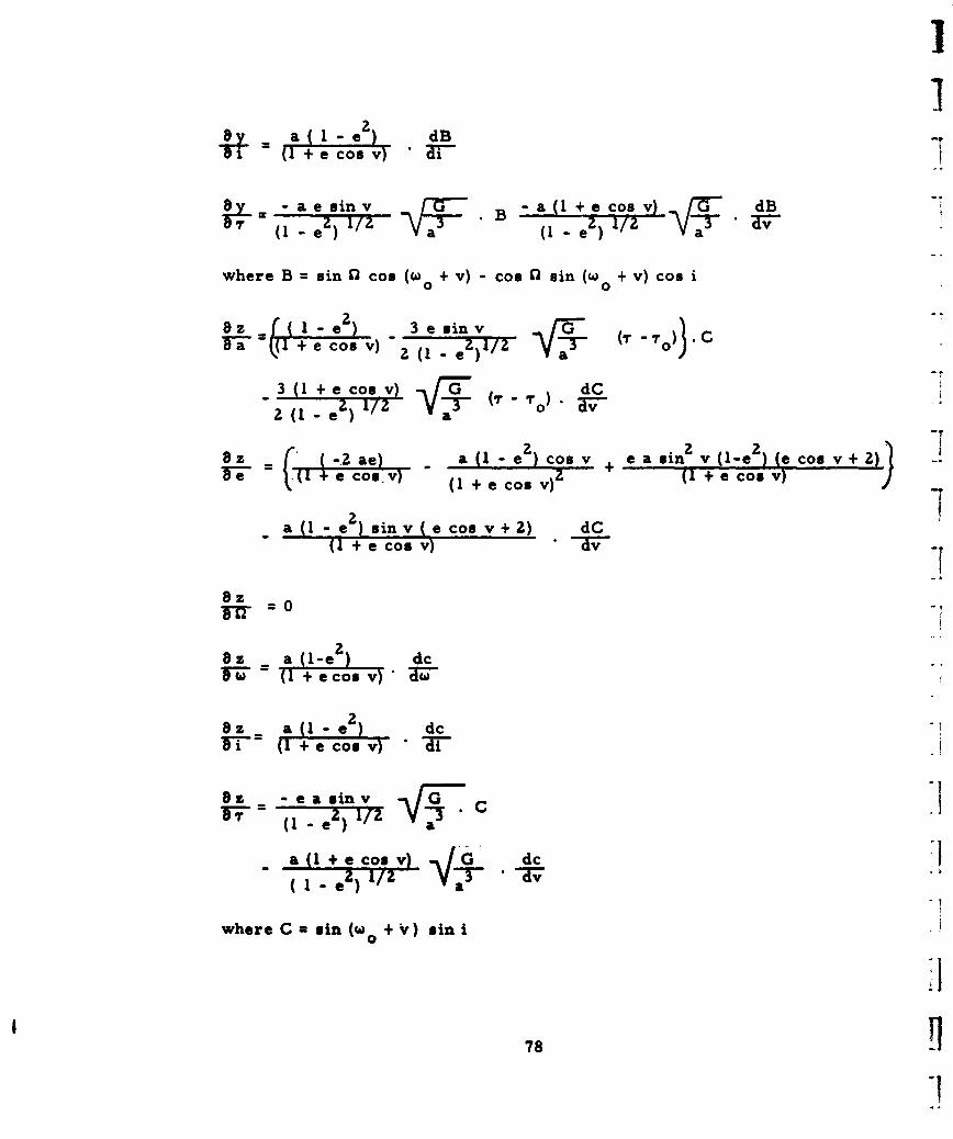
a(I I - •dB
-ae sin v a (f+ co a v) dBz 177-l i B le z z ' TV-
where B =sin 1 cos ( + v) -cos 0 sin (w + v) cos i0 0
S0 +e cos v) 2 (1 - e .I / 1 0
\+•co.v) (1 + e cos v) (+e•cos v)
aa
3a(1 + co v) dC
Bzr.,-. = 0,
1z e dc
2 ~~ 2d
= ± eosv d
2 (1-.) a
-= ( + + e co. v) + e-odT-. CsV
a I - e ) si/ v eco + ) d. II+ cos v)"l =V
+ e co v; ) / T- ""
where C sin(w +v) Gini
78
I= z T I
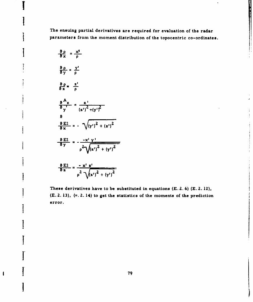
!I
The ensuing partial derivatives are required for evaluation of the radar
parameters from the moment distribution of the topocentric co-ordinates.
Xi
P
I Z
y (zt) +(y,)
a El -
SEl x z
- 2 __-_ , + __ ,
These derivatives have to be substituted in equations (E. 2. 6) (E. 2. 12),
(E. 2. 13), (=. 2. 14) to get the statistics of the moments of the prediction
error.
I
! 79
I )
Top Related