![Parallel implementation of the TRANSIMS micro … · arXiv:cs/0105004v1 [cs.CE] 2 May 2001 Parallel implementation of the TRANSIMS micro-simulation Kai Nagela ,1 and Marcus Rickertb](https://static.fdocuments.in/doc/165x107/5b5de4f37f8b9a65028e94ab/parallel-implementation-of-the-transims-micro-arxivcs0105004v1-csce-2-may.jpg)


Languages
Pages
Legal

SDS – BackgroundMathematics of SDS
Application AreasSummary
Sequential Dynamical Systems and Applications
to Biological and Socio-Technical Systems
Henning S. Mortveit
Department of Mathematics &NDSSL, Virginia Bioinformatics Institute
Virginia Polytechnic Institute and State University
December 8, 2005 / GBCB seminar

SDS – BackgroundMathematics of SDS
Application AreasSummary
Outline
SDS
1 SDS – Background
Transims – The Portland Road Network
Applications & Motivation
Definitions
2 Mathematics of SDS
Update Order Equivalence
Invertibility
Reduction
3 Application Areas
Gene Annotation & Functional Linkage Networks
Large-scale Epidemiology - EpiSims
Maximal Parallelization
SDS & Specialized Hardware Architectures
4 Summary

SDS – BackgroundMathematics of SDS
Application AreasSummary
Transims – The Portland Road NetworkTransims – DetailsApplications & MotivationDefinitions
SDS – BackgroundMathematics of SDS
Application AreasSummary
Transims – The Portland Road NetworkTransims – DetailsApplications & MotivationDefinitions
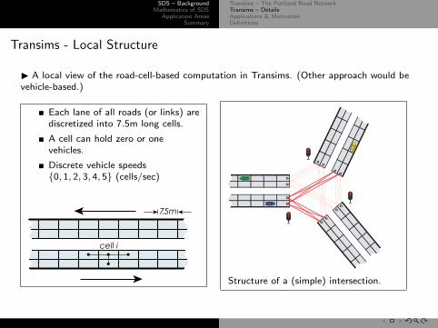
Transims - Local Structure
I A local view of the road-cell-based computation in Transims. (Other approach would bevehicle-based.)
Each lane of all roads (or links) arediscretized into 7.5m long cells.
A cell can hold zero or onevehicles.
Discrete vehicle speeds{0, 1, 2, 3, 4, 5} (cells/sec)
7.5m
cell i
Structure of a (simple) intersection.

SDS – BackgroundMathematics of SDS
Application AreasSummary
Transims – The Portland Road NetworkTransims – DetailsApplications & MotivationDefinitions
Transims micro-simulator:
Constructed from four cellular automata (CA) / SDS:
Lane change decision: Φ1
Lane Change: Φ2
Velocity update: Φ3
Position update: Φ4
The micro-simulator is the composed map: Φ4 ◦ Φ3 ◦ Φ2 ◦ Φ1

SDS – BackgroundMathematics of SDS
Application AreasSummary
Transims – The Portland Road NetworkTransims – DetailsApplications & MotivationDefinitions
Transims short movie - click to play (Note: requires quick time plug-in)
SDS – BackgroundMathematics of SDS
Application AreasSummary
Transims – The Portland Road NetworkTransims – DetailsApplications & MotivationDefinitions
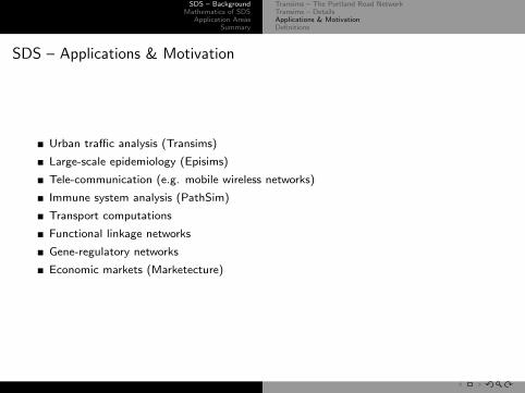
SDS – Applications & Motivation
Urban traffic analysis (Transims)
Large-scale epidemiology (Episims)
Tele-communication (e.g. mobile wireless networks)
Immune system analysis (PathSim)
Transport computations
Functional linkage networks
Gene-regulatory networks
Economic markets (Marketecture)

SDS – BackgroundMathematics of SDS
Application AreasSummary
Transims – The Portland Road NetworkTransims – DetailsApplications & MotivationDefinitions
SDS – Application Characteristics
I SDS is a class of graph dynamical systems abstracting computations in distributed,non-homogeneous systems.
I They capture:
Entities/Agents/Objects with states and local update/decision rules.
Local communication capabilities among entities.
An update mechanism scheduling the individual agent updates.
I Interpretation (a simple first-cut):
A finite undirected graph with a state associated to each vertex.
A vertex-indexed sequence of Boolean functions.
An update order/permutation of the vertices.
SDS – BackgroundMathematics of SDS
Application AreasSummary
Transims – The Portland Road NetworkTransims – DetailsApplications & MotivationDefinitions
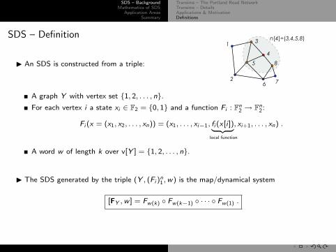
SDS – Definition
I An SDS is constructed from a triple:
2
n[4]=(3,4,5,8)1
3
5
67
8
4
A graph Y with vertex set {1, 2, . . . , n}.For each vertex i a state xi ∈ F2 = {0, 1} and a function Fi : Fn
2 → Fn2:
Fi (x = (x1, x2, . . . , xn)) = (x1, . . . , xi−1, fi (x[i ])| {z }local function
, xi+1, . . . , xn) .
A word w of length k over v[Y ] = {1, 2, . . . , n}.
I The SDS generated by the triple (Y , (Fi )n1,w) is the map/dynamical system
[FY ,w ] = Fw(k) ◦ Fw(k−1) ◦ · · · ◦ Fw(1) .
SDS – BackgroundMathematics of SDS
Application AreasSummary
Transims – The Portland Road NetworkTransims – DetailsApplications & MotivationDefinitions
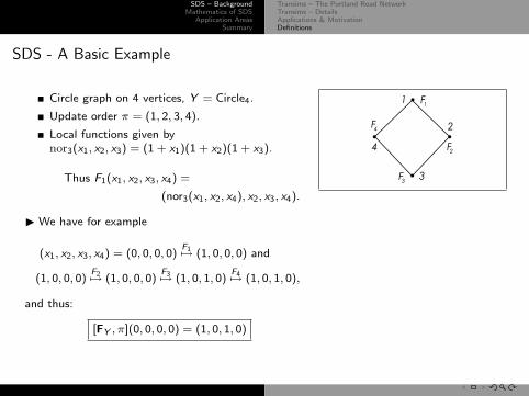
SDS - A Basic Example
Circle graph on 4 vertices, Y = Circle4.
Update order π = (1, 2, 3, 4).
Local functions given bynor3(x1, x2, x3) = (1 + x1)(1 + x2)(1 + x3).
Thus F1(x1, x2, x3, x4) =
(nor3(x1, x2, x4), x2, x3, x4).
I We have for example
(x1, x2, x3, x4) = (0, 0, 0, 0)F17→ (1, 0, 0, 0) and
(1, 0, 0, 0)F27→ (1, 0, 0, 0)
F37→ (1, 0, 1, 0)F47→ (1, 0, 1, 0),
and thus:
[FY , π](0, 0, 0, 0) = (1, 0, 1, 0)
1
2
4
F4
F1
F2
F3
3
1000
0010
0100
0001 1010
0000
0101
0011
1011
0111
1111
1101
(1234)
0110 1110
1001
1100

SDS – BackgroundMathematics of SDS
Application AreasSummary
Transims – The Portland Road NetworkTransims – DetailsApplications & MotivationDefinitions
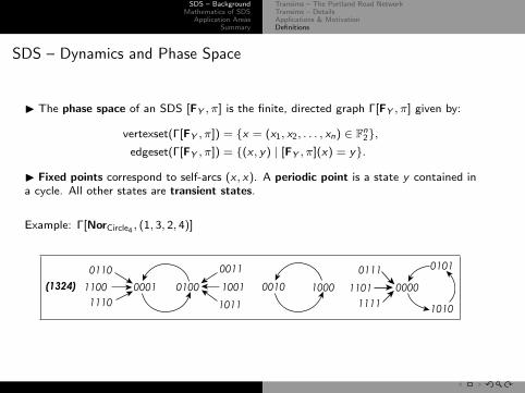
SDS – Dynamics and Phase Space
I The phase space of an SDS [FY , π] is the finite, directed graph Γ[FY , π] given by:
vertexset(Γ[FY , π]) = {x = (x1, x2, . . . , xn) ∈ Fn2},
edgeset(Γ[FY , π]) = {(x , y) | [FY , π](x) = y}.
I Fixed points correspond to self-arcs (x , x). A periodic point is a state y contained ina cycle. All other states are transient states.
Example: Γ[NorCircle4, (1, 3, 2, 4)]
0111
1111
1101
1010
0000
0101
0010 1000
1110
1100
0110 0011
1001
1011
0001 0100(1324)
SDS – BackgroundMathematics of SDS
Application AreasSummary
Transims – The Portland Road NetworkTransims – DetailsApplications & MotivationDefinitions
SDS – Dynamics and Phase Space
I The phase space of an SDS [FY , π] is the finite, directed graph Γ[FY , π] given by:
vertexset(Γ[FY , π]) = {x = (x1, x2, . . . , xn) ∈ Fn2},
edgeset(Γ[FY , π]) = {(x , y) | [FY , π](x) = y}.
I Fixed points correspond to self-arcs (x , x). A periodic point is a state y contained ina cycle. All other states are transient states.
Example: Γ[NorCircle4, (1, 3, 2, 4)]
0111
1111
1101
1010
0000
0101
0010 1000
1110
1100
0110 0011
1001
1011
0001 0100(1324)

SDS – BackgroundMathematics of SDS
Application AreasSummary
Transims – The Portland Road NetworkTransims – DetailsApplications & MotivationDefinitions
SDS – Research Approach and Questions
I Approach: Derive qualitative and quantitative infor-mation about a simulation system based on known prop-erties (e.g. Graph, Functions, Update order) withoutactually implementing and exhaustively running the fullsystem.
I Example: Fixed points, or steady states, can becomputed locally. The local fixed point candidates arepatched together to obtain system global fixed points.
w, (123...)
Global System Properties
Y,(Fi)1
n
, (Nori)1
n
Questions:
Invertibility
Equivalence
Reduction
Fixed point structure
Orbit structure
SDS – BackgroundMathematics of SDS
Application AreasSummary
Update Order EquivalenceInvertibilityReduction
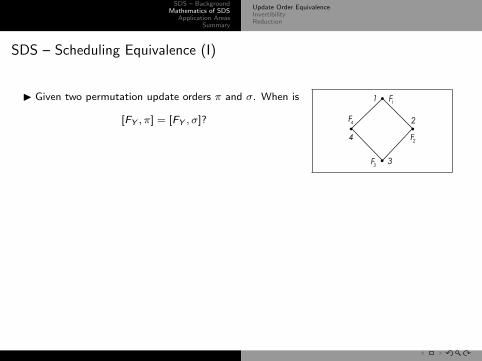
SDS – Scheduling Equivalence (I)
I Given two permutation update orders π and σ. When is
[FY , π] = [FY , σ]?
An answer is given by the update graph U(Y ). The updategraph has vertex set Sn. Two permutations are connected ifthey differ by exactly one flip of two consecutive elements iand j such that {i , j} 6∈ Y .
Proposition:i) The permutations in a component of U(Y ) all induce thesame SDS.ii) For each component in U(Y ) there is a unique acyclicorientation of Y and vice versa.iii) The maximal number of different SDS obtainable throughrescheduling is bounded above by |Acyc(Y )|. The bound isalways realized for NOR-SDS.
1
2
4
F4
F1
F2
F3
3
(1234) (2341) (3412) (4123)
(4321) (3214) (2143) (1432)
(1243) (1423) (3241) (3421)
(2134) (2314) (4132) (4312)
(1324) (3124) (2413) (4213)
(1342) (3142) (2431) (4231)
U(Circ4)
SDS – BackgroundMathematics of SDS
Application AreasSummary
Update Order EquivalenceInvertibilityReduction
SDS – Scheduling Equivalence (I)
I Given two permutation update orders π and σ. When is
[FY , π] = [FY , σ]?
An answer is given by the update graph U(Y ). The updategraph has vertex set Sn. Two permutations are connected ifthey differ by exactly one flip of two consecutive elements iand j such that {i , j} 6∈ Y .
Proposition:i) The permutations in a component of U(Y ) all induce thesame SDS.ii) For each component in U(Y ) there is a unique acyclicorientation of Y and vice versa.iii) The maximal number of different SDS obtainable throughrescheduling is bounded above by |Acyc(Y )|. The bound isalways realized for NOR-SDS.
1
2
4
F4
F1
F2
F3
3
(1234) (2341) (3412) (4123)
(4321) (3214) (2143) (1432)
(1243) (1423) (3241) (3421)
(2134) (2314) (4132) (4312)
(1324) (3124) (2413) (4213)
(1342) (3142) (2431) (4231)
U(Circ4)

SDS – BackgroundMathematics of SDS
Application AreasSummary
Update Order EquivalenceInvertibilityReduction
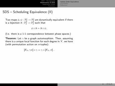
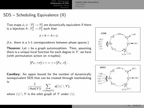
SDS – Scheduling Equivalence (II)
Two maps φ, ψ : Fn2 → Fn
2 are dynamically equivalent if thereis a bijection h : Fn
2 → Fn2 such that
φ ◦ h = h ◦ ψ.
(I.e. there is a 1-1 correspondence between phase spaces.)
Theorem: Let γ be a graph automorphism. Then, assumingthere is a unique local function for each degree in Y , we have(with permutation action on n-tuples):
[FY , γπ] ◦ γ = γ ◦ [FY , π] .
Corollary: An upper bound for the number of dynamicallynonequivalent SDS that can be created through reschedulingis:
1
|Aut(Y )|X
γ∈Aut(Y )
a(〈γ〉 \ Y ),
where 〈γ〉 \ Y is the orbit graph of Y under 〈γ〉.
1000
0010
0100
0001 1010
0000
0101
0011
1011
0111
1111
1101
(1234)
0110 1110
1001
1100
0001
0100
0010
10000101
0000
1010
1100
1101
1110
1111
1011
(4321)
01100111
1001
0011
SDS – BackgroundMathematics of SDS
Application AreasSummary
Update Order EquivalenceInvertibilityReduction
SDS – Scheduling Equivalence (II)
Two maps φ, ψ : Fn2 → Fn
2 are dynamically equivalent if thereis a bijection h : Fn
2 → Fn2 such that
φ ◦ h = h ◦ ψ.
(I.e. there is a 1-1 correspondence between phase spaces.)
Theorem: Let γ be a graph automorphism. Then, assumingthere is a unique local function for each degree in Y , we have(with permutation action on n-tuples):
[FY , γπ] ◦ γ = γ ◦ [FY , π] .
Corollary: An upper bound for the number of dynamicallynonequivalent SDS that can be created through reschedulingis:
1
|Aut(Y )|X
γ∈Aut(Y )
a(〈γ〉 \ Y ),
where 〈γ〉 \ Y is the orbit graph of Y under 〈γ〉.
1000
0010
0100
0001 1010
0000
0101
0011
1011
0111
1111
1101
(1234)
0110 1110
1001
1100
0001
0100
0010
10000101
0000
1010
1100
1101
1110
1111
1011
(4321)
01100111
1001
0011
SDS – BackgroundMathematics of SDS
Application AreasSummary
Update Order EquivalenceInvertibilityReduction
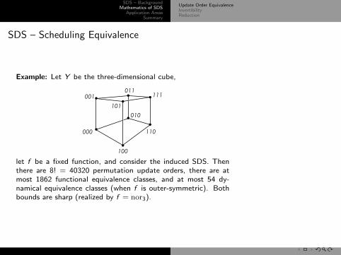
SDS – Scheduling Equivalence
Example: Let Y be the three-dimensional cube,
000
100
110
010
111
101
001
011
let f be a fixed function, and consider the induced SDS. Thenthere are 8! = 40320 permutation update orders, there are atmost 1862 functional equivalence classes, and at most 54 dy-namical equivalence classes (when f is outer-symmetric). Bothbounds are sharp (realized by f = nor3).
SDS – BackgroundMathematics of SDS
Application AreasSummary
Update Order EquivalenceInvertibilityReduction
SDS – Scheduling Equivalence (III)
I Sketch of proof: [FY , γπ] = γ ◦ [FY , π] ◦ γ−1
I Rewrite, expand and compare ith factor on both sides:
LHS:Fγπ(i)(x) = (x1, . . . , fγπ(i)(xk |k ∈ B1(γπ(i)))| {z }
pos. γπ(i)
, . . . , xn)
RHS:
(γ ◦ Fπ(i) ◦ γ−1)(x) = (γ ◦ Fπ(i))(xγ(1), . . . , xγ(n))
= γ(xγ(1), . . . , fπ(i)(xk |k ∈ γB1(π(i)))| {z }pos. π(i)
, . . . , xγ(n))
= (x1, . . . , fπ(i)(xk |k ∈ γB1(π(i)))| {z }pos. γπ(i)
, . . . , xn)

SDS – BackgroundMathematics of SDS
Application AreasSummary
Update Order EquivalenceInvertibilityReduction
Invertible/Reversible SDS
Invertibility of an SDS [FY ,w ] depends only on the functions fi .
Sufficient and necessary condition: Each partial map fi (−, x ′[i ]) : F2 → F2 is a bijection foreach choice of sub-configuration x ′[i ].
Differs from CA where invertibility also depends on the graph & the number of vertices.
Proposition: If [FY ,w ] is a Boolean, invertible SDS with symmetric functions fi thenfi (x1, . . . , xk ) = parity(x1, . . . , xk ) = x1 + · · ·+ xk or fi (x1, . . . , xk ) = 1 + parity(x1, . . . , xk ).
Proof idea: The conditions of binary, invertible and symmetric determines fi by its value on thestate (0, 0, . . . , 0).
A generalization:
Proposition: Let A = {0, 1, . . . , k − 1}. A totalistic function f : Ak → A of an invertible SDS iscompletely determined by its value on distance classes 0, 1, . . . , k − 2.
SDS – BackgroundMathematics of SDS
Application AreasSummary
Update Order EquivalenceInvertibilityReduction
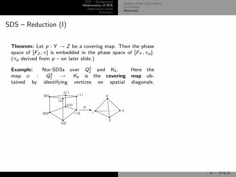
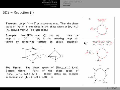
SDS – Reduction (I)
Theorem: Let p : Y → Z be a covering map. Then the phasespace of [FZ , π] is embedded in the phase space of [FY , πp].(πp derived from p – on later slide.)
Example: Nor-SDSs over Q32 and K4. Here the
map φ : Q32 → K4 is the covering map ob-
tained by identifying vertices on spatial diagonals.
p
000
100
110
010
111
101
001011
1
2
3
4
Top figure: The phase space of [NorK4, (1, 2, 3, 4)].
Bottom figure: Parts of the phase space of[NorK4
, (0, 7, 1, 6, 2, 5, 3, 4)]. Binary states are encodedin decimal, e.g. (1, 1, 0, 0, 0, 0, 0, 0) 7→ 3.
0
60,90,126,153,
189,219,255
129
6636
195
K4
102,
165,231
24
0
25,...,59,60,61,...,90,91,...,125,
126,127,152,153,154,...,188,189,
190,...,218,219,220,...,254,255
129
6636
67,194,195
37,...,101,
102,103,164,
165,...,230,231
24
1
131
Q2
3
232
52,53,54,...136
97,98,99,....
21
130
20
97 8
150
104
SDS – BackgroundMathematics of SDS
Application AreasSummary
Update Order EquivalenceInvertibilityReduction
SDS – Reduction (I)
Theorem: Let p : Y → Z be a covering map. Then the phasespace of [FZ , π] is embedded in the phase space of [FY , πp].(πp derived from p – on later slide.)
Example: Nor-SDSs over Q32 and K4. Here the
map φ : Q32 → K4 is the covering map ob-
tained by identifying vertices on spatial diagonals.
p
000
100
110
010
111
101
001011
1
2
3
4
Top figure: The phase space of [NorK4, (1, 2, 3, 4)].
Bottom figure: Parts of the phase space of[NorK4
, (0, 7, 1, 6, 2, 5, 3, 4)]. Binary states are encodedin decimal, e.g. (1, 1, 0, 0, 0, 0, 0, 0) 7→ 3.
0
60,90,126,153,
189,219,255
129
6636
195
K4
102,
165,231
24
0
25,...,59,60,61,...,90,91,...,125,
126,127,152,153,154,...,188,189,
190,...,218,219,220,...,254,255
129
6636
67,194,195
37,...,101,
102,103,164,
165,...,230,231
24
1
131
Q2
3
232
52,53,54,...136
97,98,99,....
21
130
20
97 8
150
104

SDS – BackgroundMathematics of SDS
Application AreasSummary
Update Order EquivalenceInvertibilityReduction
SDS – Reduction (II) – Example
I Proposition: Let n ≥ 3 and assume 2n ≡ 0 mod n + 1. Then there exists acovering map φ : Qn
2 −→ Kn+1, and any SDS of the form [ParityQn2, ηφ(π)] with
π ∈ Sn+1 has a periodic orbit of length n + 2.
I Idea: Analyze the Parity system over the complete graph – then use thetheorem and the embedding.

SDS – BackgroundMathematics of SDS
Application AreasSummary
Update Order EquivalenceInvertibilityReduction
SDS – Reduction (III)
I A covering map p : Y → Z induces:
A state map: χp : F|Z |2 → F|Y |2 , where (χp(x))i = xp(i)
A map of update orders: ηp : S|Z | → S|Y |, where πηp7→ πp (“concatenate” the p−1(πi )’s)
I Observation: For a covering map p the set p−1(i) is an independent set of Y .
I Implication: We have a commutative diagram:
x //
χp
��
Fk,Z (x)
χp
��w //
Qi∈p−1(k)
Fi,Y (w)
By composition:
χp ◦ [FZ , π] = [FY , πp] ◦ χp

SDS – BackgroundMathematics of SDS
Application AreasSummary
Gene Annotation & Functional Linkage NetworksLarge-scale Epidemiology - EpiSimsMaximal ParallelizationSDS & Specialized Hardware Architectures
Functional Linkage Networks
I Goal: Determine if a collection of genes have some set of biological functions.
Modeling approach:
Represent genes as nodes and connect genes if there is experimental/computationalevidence indicating that they share some given biological function.
Assign a state +1 to genes that have function f (are annotated by the function f ) and −1to genes that do not have function f . Assign state 0 to states of remaining nodes.
Each edge e has a weight we ∈ [−1, 1]. (sign: + share/ − don’t share function f ,magnitude reflects certainty)
Goal: Given network and initial configuration x = (xu)u∈v[Y ] assign states ±1 to all the geneswith state 0 so as to minimize the energy function
E(x ,Y ) = −X
{u,v}∈e[Y ]
w{u,v}xuxv .
Observation: Locally, neighbor genes with identical states should be connected by a positiveedge and neighbor genes with opposite states should be connected by a negative edge.
(Work with T. M. Murali)
SDS – BackgroundMathematics of SDS
Application AreasSummary
Gene Annotation & Functional Linkage NetworksLarge-scale Epidemiology - EpiSimsMaximal ParallelizationSDS & Specialized Hardware Architectures
Functional Linkage Networks - (II)
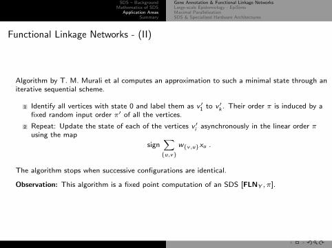
Algorithm by T. M. Murali et al computes an approximation to such a minimal state through aniterative sequential scheme.
1 Identify all vertices with state 0 and label them as v ′1 to v ′k . Their order π is induced by afixed random input order π′ of all the vertices.
2 Repeat: Update the state of each of the vertices v ′i asynchronously in the linear order πusing the map
signX{u,v}
w{v,u}xu .
The algorithm stops when successive configurations are identical.
Observation: This algorithm is a fixed point computation of an SDS [FLNY , π].
SDS – BackgroundMathematics of SDS
Application AreasSummary
Gene Annotation & Functional Linkage NetworksLarge-scale Epidemiology - EpiSimsMaximal ParallelizationSDS & Specialized Hardware Architectures
Functional Linkage Networks - (III)
Facts: The SDS [FLNY , π] has only fixed points as attractors (i.e. no periodic orbits of period≥ 2.) Proof idea: Every state transition lowers the energy.
Ongoing work:
Understand number and structure of fixed points. (The set of fixed points to do notdepend on the update order.)
Understand relation attractor structure and the update order π.
Analysis through random graph models.
SDS – BackgroundMathematics of SDS
Application AreasSummary
Gene Annotation & Functional Linkage NetworksLarge-scale Epidemiology - EpiSimsMaximal ParallelizationSDS & Specialized Hardware Architectures
EpiSims
I Overview:
Project led by Stephen Eubank, NDSSL.
A model and tool for analysis of epidemiology in social networks.
High level of resolution (no mixing assumption as in ODE/PDE type models)
Is implemented as a probabilistic, discrete event simulation with parametrized individuals.
Modeled on top of a population mobility module (e.g. TRANSIMS).
Case studies for Influenza and Smallpox.
I Applications & usage:
Scenario studies (population vulnerability, propagation speed.)
Study effects of vaccination policies and general intervention strategies.

SDS – BackgroundMathematics of SDS
Application AreasSummary
Gene Annotation & Functional Linkage NetworksLarge-scale Epidemiology - EpiSimsMaximal ParallelizationSDS & Specialized Hardware Architectures
EpiSims - Details
Individuals mapped to activity locations by mobility module.
Basic steps: 1) S → I , and 2) individual disease evolution:
Infected
Individual disease evolution.
A probabilistic FSM.
Susceptible
S → I : Bernoulli trials using probability
pi,s,a =n
1− expˆt
Xj∈TI
Xr∈R(j)
Nj,r ln(1− rs ρa(i , j))˜o.
Mα .
In the infected state the disease evolution is governed by probabilistic finite state machine.
I A discrete, finite (probabilistic) dynamical system.
I Are studying simpler SIR models using SDS/CA.
Questions: What is the structure and properties of the social network graph? How does thisinfluence evolution?

SDS – BackgroundMathematics of SDS
Application AreasSummary
Gene Annotation & Functional Linkage NetworksLarge-scale Epidemiology - EpiSimsMaximal ParallelizationSDS & Specialized Hardware Architectures
Parallelization in Transport Computations
Application: Transport Codes
Unstructured tetrahedral mesh & direction −→task dependency digraph
One pass of numerical transport code ←→sequential dynamical system
In general: N interdependent tasks ordered by aDAG distributed on M processors. Goal: Fastexecution.
An optimization problem over a component in theSDS update graph!
Induced DigraphUnstructured Mesh
T2
T1
T2
T1
τ1
τ4τ3
τ2
τ1 τ4τ2 τ3
Pass 1 1 -Pass 2 - 4Pass 3 - 3Pass 4 2 -
τ1 τ3τ2 τ4
Pass 1 1 -Pass 2 - 3Pass 3 2 4Pass 4 - -

SDS – BackgroundMathematics of SDS
Application AreasSummary
Gene Annotation & Functional Linkage NetworksLarge-scale Epidemiology - EpiSimsMaximal ParallelizationSDS & Specialized Hardware Architectures
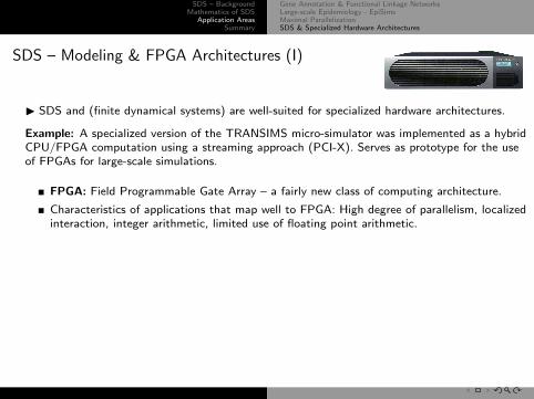
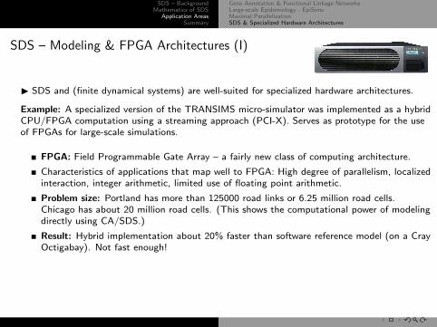
SDS – Modeling & FPGA Architectures (I)
I SDS and (finite dynamical systems) are well-suited for specialized hardware architectures.
Example: A specialized version of the TRANSIMS micro-simulator was implemented as a hybridCPU/FPGA computation using a streaming approach (PCI-X). Serves as prototype for the useof FPGAs for large-scale simulations.
FPGA: Field Programmable Gate Array – a fairly new class of computing architecture.
Characteristics of applications that map well to FPGA: High degree of parallelism, localizedinteraction, integer arithmetic, limited use of floating point arithmetic.
Problem size: Portland has more than 125000 road links or 6.25 million road cells.Chicago has about 20 million road cells. (This shows the computational power of modelingdirectly using CA/SDS.)
Result: Hybrid implementation about 20% faster than software reference model (on a CrayOctigabay). Not fast enough!
Lessons learnt: Both Design and Implementations of large-scale simulations likeTRANSIMS need to be done with specialized hardware in mind. The“optimize-the-inner-loop” afterthought will not cut it.(note: redundant computation through overlapping domain decomposition)
SDS – BackgroundMathematics of SDS
Application AreasSummary
Gene Annotation & Functional Linkage NetworksLarge-scale Epidemiology - EpiSimsMaximal ParallelizationSDS & Specialized Hardware Architectures
SDS – Modeling & FPGA Architectures (I)
I SDS and (finite dynamical systems) are well-suited for specialized hardware architectures.
Example: A specialized version of the TRANSIMS micro-simulator was implemented as a hybridCPU/FPGA computation using a streaming approach (PCI-X). Serves as prototype for the useof FPGAs for large-scale simulations.
FPGA: Field Programmable Gate Array – a fairly new class of computing architecture.
Characteristics of applications that map well to FPGA: High degree of parallelism, localizedinteraction, integer arithmetic, limited use of floating point arithmetic.
Problem size: Portland has more than 125000 road links or 6.25 million road cells.Chicago has about 20 million road cells. (This shows the computational power of modelingdirectly using CA/SDS.)
Result: Hybrid implementation about 20% faster than software reference model (on a CrayOctigabay). Not fast enough!
Lessons learnt: Both Design and Implementations of large-scale simulations likeTRANSIMS need to be done with specialized hardware in mind. The“optimize-the-inner-loop” afterthought will not cut it.(note: redundant computation through overlapping domain decomposition)

SDS – BackgroundMathematics of SDS
Application AreasSummary
Outlook, Research DirectionsCollaborators, students, papers, info
SDS – Current Research Directions
Stochastic SDS: By allowing stochastic e.g. functions, states or edges onenaturally induce random (di)graph models which again induce Markov chains.Needed for modeling many applications. Can be used to study for example longterm behavior in the presence of noise and stable computation. (NSF × 2).
Compositions of SDS as they occur in for example the TRANSIMSmicro-simulator. Hierarchical SDS in general.
Discrete Derivative for SDS: Extend work done in e.g. switching theory (Thayse),preliminary results for CA (Vichniac), and work by Bazso to SDS. Goal: Derive acomputationally efficient operator or tool that allow us to derive dynamicsproperties without resorting to exhaustive computation. Problems: Chain rules andproduct rules are complex (no lim
h→0and vanishing terms), and SDS are in general
deeply nested/composed maps.
SDS with word update orders. Initial work has revealed additional structures thatare trivial in the case of permutations. Analysis and extension of previous resultsfar from straight-forward.

SDS – BackgroundMathematics of SDS
Application AreasSummary
Outlook, Research DirectionsCollaborators, students, papers, info
SDS – Collaborators, Papers, Info
Collaborators: Christian M. Reidys, Chris L. Barrett, Reinhard Laubenbacher, Bodo Pareigis,Madhav Marathe, Anil Vullikanti, T.M. Murali, Maya Gokhale, Justin Tripp.
Students: Mariana Raykova, Matt Macauley.
Mortveit, H. S. and Reidys, C. M. ”Discrete, sequential dynamical systems”, DiscreteMathematics, 2001 (226):281–295.
A. A. Hansson, Mortveit, H. S. and Reidys, C. M. ”On Asynchronous Cellular Automata”,”Advances in Complex Systems”, in press.
Barrett, C. L., Mortveit, H. S. and Reidys, C. M. ”Elements of a theory of simulation III:Equivalence of SDS”, Appl. Math. and Comput., 2001 (122):325–340.
Mortveit, H. S. and Reidys, C. M. ”Reduction of Discrete Dynamical Systems overGraphs”, Advances in Complex Systems, vol 7, No. 1, 2004, 1–20.
Web: http://ndssl.vbi.vt.edu
Top Related