


Languages
Pages
Legal


Article
Sensitive SurveyQuestions withAuxiliary Information
Winston Chou1, Kosuke Imai2
and Bryn Rosenfeld3
Abstract
Scholars increasingly rely on indirect questioning techniques to reduce socialdesirability bias and item nonresponse for sensitive survey questions. Themajor drawback of these approaches, however, is their inefficiency relativeto direct questioning. We show how to improve the statistical analysis ofthe list experiment, randomized response technique, and endorsementexperiment by exploiting auxiliary information on the sensitive trait. Weapply the proposed methodology to survey experiments conducted amongvoters in a controversial antiabortion referendum held during the 2011Mississippi General Election. By incorporating the official county-levelelection results, we obtain precinct- and individual-level estimates that aremore accurate than standard indirect questioning estimates and occasionallyeven more efficient than direct questioning. Our simulation studies shed lighton the conditions under which our approach can improve the efficiency androbustness of estimates based on indirect questioning techniques. Open-source software is available for implementing the proposed methodology.
1 Department of Politics, Princeton University, Princeton, NJ, USA2 Department of Politics, Center for Statistics and Machine Learning, Princeton University,
Princeton, NJ, USA3 Department of Political Science, University of Southern California, Los Angeles, CA, USA
Corresponding Author:
Kosuke Imai, Princeton University, Princeton, NJ 08544, USA.
Email: [email protected]
Sociological Methods & Research1-37
ª The Author(s) 2017Reprints and permission:
sagepub.com/journalsPermissions.navDOI: 10.1177/0049124117729711
journals.sagepub.com/home/smr
Keywords
endorsement experiment, item count technique, list experiment, rando-mized response technique, social desirability bias, survey experiment,unmatched count technique
Introduction
While many social scientists use surveys to measure individual opinion and
behavior on a range of sensitive topics, including racial discrimination,
corruption, drug use, and sexual behavior, the validity of survey measure-
ments is often compromised by misreporting and nonresponse. Scholars
increasingly rely on indirect questioning techniques to alleviate such bias
(e.g., Gingerich 2010; Gonzalez-Ocantos et al. 2012; Janus 2010; Krumpal
2012; Kuklinski, Cobb, and Gilens 1997; Lyall, Blair, and Imai 2013). Three
survey methodologies that have recently attracted much attention are the list
experiment (also known as item/unmatched count technique), randomized
response technique, and endorsement experiment. These techniques seek to
elicit truthful answers to sensitive survey questions by obscuring individual
responses, thus affording respondents greater privacy. Some validation stud-
ies have found that indirect questioning techniques can significantly reduce
bias relative to direct questioning (e.g., Coutts and Jann 2011; Rosenfeld,
Imai, and Shapiro 2016; van der Heijden et al. 2000), though others report
more pessimistic results (e.g., Wolter and Preisendorfer 2013).
Despite their promise and increasing popularity, the major drawback of
indirect questioning techniques is that the resulting estimates are often much
less efficient than those obtained under direct questioning. Therefore, the
bias reduction may be offset by an increase in variance. Although scholars
have developed new multiple regression techniques (see Blair and Imai
2012; Blair, Imai, and Zhou 2015; Bullock, Imai, and Shapiro 2011, and
references therein) and proposed to combine multiple direct/indirect ques-
tioning techniques (Aronow et al. 2015; Blair, Imai, and Lyall 2014), these
new methods often fail to fundamentally overcome the problem of efficiency
loss inherent in indirect questioning. As a result, a considerably greater
number of respondents are required to obtain precise estimates through indi-
rect questioning techniques.
In this article, we show how to improve the statistical analysis of indirect
questioning techniques by exploiting auxiliary information about the preva-
lence of sensitive traits in the population under study. Information of this
kind can come from many sources, including censuses, administrative
records, and expert evaluations, and is often available for topics that are
2 Sociological Methods & Research XX(X)

sensitive and private in nature, such as turnout and voter choice (Karp and
Brockington 2005), disease prevalence (Martin et al. 2000), income (Kim
and Tamborini 2014; Schrapler 2004), unlawful or fraudulent behavior (van
der Heijden et al. 2000), and contact with the criminal justice system
(Kling, Ludwig, and Katz 2005; Wolter and Preisendorfer 2013; Wyner
1980). The key characteristic of the auxiliary information we consider is
that, although a reliable measure of the sensitive trait is unavailable at the
individual level, the same trait can be measured fairly accurately at an
aggregate level. We demonstrate that such aggregate information can be
harnessed in multivariate analyses to sharpen inference about the relation-
ships between sensitive traits and other characteristics of individuals and in
hierarchical analyses to generate more accurate estimates of the prevalence
of sensitive traits in subpopulations.
In addition, combining individual- and aggregate-level information can
reduce the potential bias of sensitive survey techniques. Bias reduction is an
important consideration because sensitive survey techniques are not guaran-
teed to produce valid estimates (e.g., Wolter and Preisendorfer 2013). We
construct individual-level estimates such that they are consistent with true
aggregate-level information. This approach has been used elsewhere. For
example, to overcome the fundamental difficulty of inferring individual
behavior from aggregate data (Cross and Manski 2002; Duncan and Davis
1953), the recent literature on ecological inference proposes to incorporate
individual-level information (e.g., Greiner and Quinn 2010; Imai and Khanna
2016). We show that this approach is also effective for improving the esti-
mates from sensitive survey techniques.
In the second section, we first show how to incorporate auxiliary infor-
mation into statistical analyses of the list experiment and randomized
response technique. This is done by applying the generalized method of
moments approach (e.g., Handcock, Rendall, and Cheadle 2005; Hellerstein
and Imbens 1999; Imbens and Lancaster 1994) to the multiple regression
models of Imai (2011) and Blair et al. (2015). For the endorsement experi-
ment, we embed auxiliary information in the Bayesian hierarchical model of
Bullock et al. (2011) through the specification of the prior distribution. In all
cases, the proposed methodology does not modify the original multiple
regression models. Instead, auxiliary information is represented either as
additional moment conditions (for the list experiment and randomized
response technique) or as prior distributions (for the endorsement experi-
ment). Thus, the interpretation of the fitted models remains unchanged.
In the third section, we apply the proposed methodology to survey experi-
ments on an antiabortion referendum in the 2011 Mississippi General
Chou et al. 3

Election. Rosenfeld et al. (2016) administered and analyzed these experi-
ments for the purpose of validating the accuracy of the list experiment,
randomized response technique, and endorsement experiment. We incorpo-
rate the county-level official election results as auxiliary information and
examine how each indirect questioning technique fares in recovering the
sensitive trait at a lower level of aggregation. Specifically, we use
precinct-level official election results on the sensitive referendum as a known
benchmark to demonstrate the efficacy of our proposed approach. The avail-
ability of precinct-level results allows us to validate our methods.
Using this validation study, we find that auxiliary information substan-
tially improves prediction: incorporating county-level election results
reduces the root mean square error (RMSE) of precinct-level predictions
by up to 60 percent and more than doubles the correlation between the
estimates and their corresponding truths. We also find that incorporating
auxiliary information substantially increases the statistical efficiency of
indirect questioning estimators, at times even surpassing that of direct
questioning.1
At the individual level, we find that auxiliary information also improves
the efficiency of regression coefficient estimates, revealing statistically sig-
nificant differences in support for abortion across partisan affiliation and
educational attainment. We view this as encouraging evidence for the utility
of our method, as partisanship and higher education are among the strongest
predictors of abortion attitudes in research based on efficient but potentially
biased direct questioning (e.g., Adams 1997). By contrast, the initial analysis
of our data by Rosenfeld et al. (2016) did not reveal statistically significant
differences in partisanship or education due to the greater standard error of
indirect questioning, though indirect techniques did achieve less biased esti-
mates overall. By incorporating auxiliary information, we are thus able to
mitigate one of the major drawbacks associated with indirect questioning
techniques: their inefficiency relative to direct questioning.
In the fourth section, we conduct simulation studies to explore the con-
ditions under which the proposed methodology is effective for improving
inference about multivariate relationships. We find that our method is most
effective when respondent characteristics vary greatly across groups such
as states, counties, and precincts—that is, when respondents are highly
segregated. Intuitively, when respondents who differ along a covariate are
perfectly segregated, the group-level information conveys precise knowl-
edge about the aggregate relationship between that covariate and the sen-
sitive trait. However, when respondents are less segregated, the proposed
methodology mainly improves inference for the intercept in multiple
4 Sociological Methods & Research XX(X)

regression models. Our method is also less effective when covariates are
highly correlated. Finally, the fifth section provides concluding remarks.
The proposed methodology is implemented via the open-source statistical
software, endorse: R Package for Analyzing Endorsement Experiments
(Shiraito and Imai 2015), list: Statistical Methods for the Item Count
Technique and List Experiment (Blair and Imai 2016), and rr: Statistical
Methods for the Randomized Response Technique (Blair, Zhou, and Imai
2016), all of which are available through the Comprehensive R Archive
Network (http://cran.r-project.org/).
The Proposed Methodology
In this section, we propose a new methodology that enables researchers to
incorporate auxiliary information into the statistical analysis of the list
experiment, randomized response technique, and endorsement experiment.
Here, we show how to exploit the availability of auxiliary information on the
outcome variable at an aggregate level and improve multiple regression
analyses performed at a lower level of aggregation. Specifically, we repre-
sent auxiliary information as additional moment conditions for the multi-
variate analyses of the list experiment and randomized response technique.
For the endorsement experiment, we incorporate it as part of the prior dis-
tribution for the Bayesian hierarchical measurement model. We use the
Mississippi study (Rosenfeld et al. 2016) as a running example, but a similar
methodological approach can be applied to different designs of these indirect
questioning techniques.
List Experiment
The list experiment obscures individual responses by aggregating the sensi-
tive trait with other control traits. The standard list experiment design begins
by randomly dividing a sample of N respondents into two groups. The
respondents in the control group (Ti ¼ 0) are presented with a list of J
control traits and asked to report the number of traits they possess (Yi). The
respondents in the treatment group (Ti ¼ 1) are then given the same list of J
control items plus the sensitive item and asked how many of the items they
would answer in the affirmative (Yi). The prevalence of the sensitive item is
then gauged by subtracting the mean of the control group from the mean of
the treatment group, that is, 1N1
PNi ¼ 1TiYi � 1
N�N1
PNi ¼ 1ð1� TiÞYi where
N1 ¼PN
i ¼ 1Ti.
Chou et al. 5

In the Mississippi study, the respondents in the control group were asked
the following question:
Here is a list of four things that some people have done and some people have
not. Please listen to them and then tell me HOW MANY of them you have done
in the past two years. Do not tell me which you have and have not done. Just
tell me how many:
� discussed politics with family or friends,
� cast a ballot for Governor Phil Bryant,
� paid dues to a union, and
� given money to a Tea Party candidate or organization.
How many of these things have you done in the past two years?
For the treatment group, the same script was used with the following addi-
tional sensitive item.
� Voted “yes” on the “personhood” initiative on the November 2011 Mis-
sissippi General Election ballot.
Our proposed methodology for incorporating auxiliary information into mul-
tivariate analyses of the list experiment is based on the fact that it can be
analyzed within the method of moments framework (Imai 2011). Thus, aux-
iliary information can be represented as additional moment conditions (e.g.,
Imbens and Lancaster 1994). Specifically, let Y �i 2 f0; 1; . . . ; Jg represent
the number of control traits for individual i and Zi 2 f0; 1g represent a
binary indicator variable for the sensitive trait. Then, based on the relation-
ship Yi ¼ Y �i þ TiZi, we consider the following nonlinear regression
model:
EðYijTi;XiÞ ¼ f ðXi; γÞ þ TigðXi; δÞ; ð1Þ
where f ðx; γÞ ¼ EðY �i jXi ¼ xÞ represents the average number of control
traits for individuals whose observed characteristics are given by Xi ¼ x,
gðx; δÞ ¼ PrðZi ¼ 1jXi ¼ xÞ represents the probability of an affirmative
answer to the sensitive item for the same group of individuals, and ðγ ; δÞ. is
a vector of unknown parameters. Imai (2011) suggests a two-step procedure
for fitting this model. In the first step, g is estimated using the control group
via nonlinear least squares. In the second step, δ is estimated using the
treatment group through the nonlinear least squares regression of the adjusted
response variable Yi � f ðXi; γÞ on gðXi; δÞ. We then adjust standard errors
to account for the uncertainty from the two steps.
6 Sociological Methods & Research XX(X)

In this article, we exploit auxiliary information about the population mean
of the sensitive trait for different groups. In our empirical example, we use
the aggregate official election results, which contain the population propor-
tion of yes votes in each of 19 counties in Mississippi, in order to improve the
multivariate analyses of the list experiment carried out among a sample of
voters. Formally, we assume knowledge of the following moments:
PrðZi ¼ 1jGi ¼ kÞ ¼ hk ; ð2Þ
for each k 2 f1; 2; . . . ;Kg where Gi represents groups for which the aux-
iliary information is available.2
To incorporate the auxiliary information given in equation (2), we con-
sider the following moment condition:
1
N
XN
i¼1
1fGi ¼ kgfgðXi; δÞ � hkg ¼ 0 ð3Þ
for each k 2 f1; 2; . . . ;Kg where K is the total number of groups. This
moment condition is based on the assumption that the parameter δ does not
differ across groups. The assumption can be tested using the overidentifica-
tion test based on the w2 reference distribution (Hansen 1982).3
Using equation (3) as an additional moment condition, we obtain the
following generalized method of moments (GMM) estimator of ðγ ; δÞ:
ðγ ; δÞ ¼ argminγ ; δ
lðY;X;T; γ ; δÞTcW�1lðY;X;T; γ ; δÞ; ð4Þ
where lðY;X;T; γ ; δÞ is defined by
lðY;X;T; γ ; δÞ ¼
1
N
Xn
i¼1
TifYi � f ðXi; γÞ � gðXi; δÞgg0 ðXi; δÞ
1
N
Xn
i¼1
ð1� TiÞfYi � f ðXi; γÞgf0 ðXi; γÞ
1
N
XN
i¼1
1fGi ¼ 1gfgðXi; δÞ � h1g
..
.
1
N
XN
i¼1
1fGi ¼ KgfgðXi; δÞ � hKg
266666666666666666664
377777777777777777775
; ð5Þ
Chou et al. 7

andcW is a positive semidefinite weighting matrix. Under standard regularity
conditions, this GMM estimator is consistent with any choice of cW: The
efficient GMM estimator uses a consistent estimate of the asymptotic var-
iance of lðY;X;T; γ ; δÞ as the weighting matrix. In our simulations, we
estimate the efficient weighting matrix simultaneously with the parameters.
This approach often results in lower bias and more reliable coverage rates in
finite samples (Hansen, Heaton, and Yaron 1996).
We have assumed that the population-level moments are known exactly.
This assumption is appropriate for our application. However, in many cir-
cumstances, researchers may be concerned about the accuracy of auxiliary
information and are not willing to assume that the population moments are
known exactly. In such situations, we can specify a variance for the
population-level moments in the GMM framework (Imbens and Lancaster
1994). Alternatively, we can conduct a sensitivity analysis by specifying a
plausible range of values in order to examine the robustness of the resulting
estimates to measurement error in auxiliary information.
Finally, an alternative strategy is to simply incorporate the auxiliary
information as a covariate. Although straightforward to implement, this
approach does not ensure that the model is consistent with the known pre-
valence at an aggregate level and hence cannot reduce bias. It also does not
yield a statistical test that can be used to gauge whether modeling assump-
tions are appropriate. By contrast, our approach ensures that the predicted
aggregate prevalence based on the model is consistent with the true preva-
lence (and if not, the overidentifying restriction test will be able to detect
such a model misspecification). Thus, from a theoretical perspective, our
approach is better suited to the present setting. In Online Appendix A, we
also conduct an empirical comparison between our methodology and this
alternative approach.
Randomized Response Technique
The randomized response technique, originally proposed by Warner
(1965), obscures individual responses by adding random noise to respon-
dents’ answers (see Blair et al. 2015, for a recent review). Under the “forced
response” design, respondents are asked to use a randomization device,
such as a coin flip, whose outcome is unobserved by the researcher. The
randomization device determines whether the respondent is asked to
answer the sensitive item truthfully or to reply with a forced answer, either
“yes” or “no.” This technique affords the respondent some privacy because
8 Sociological Methods & Research XX(X)

the enumerator is unsure if any individual response represents a truthful
answer or a forced response.
In the Mississippi study, the following script was used to administer the
randomized response technique, which included one practice round. Notice
that, if a respondent answered the sensitive question affirmatively, the enu-
merator would not have been able to tell whether her response represented
the outcome of a coin flip or an honest answer.4
To answer this question, you will need a coin. Once you have found one, please
toss the coin two times and note the results of those tosses (heads or tails) one
after the other on a sheet of paper. Do not reveal to me whether your coin lands
on heads or tails. After you have recorded the results of your two coin tosses,
just tell me you are ready, and we will begin.
First, we will practice. To ensure that your answer is confidential and
known only to you, please answer “yes” if either your first coin toss came
up heads or you voted in the November 2011 Mississippi General Election,
otherwise answer “no.”
Now, please answer “yes” if either your second coin toss came up heads or
you voted “yes” on the “personhood” initiative, which appeared on the Novem-
ber 2011 Mississippi General Election ballot.
As in the List Experiment subsection, let Zi represent the latent response to
the sensitive question for respondent i. We use the same parametric model as
the one used for the list experiment,
PrðZi ¼ 1jXiÞ ¼ gðXi; δÞ; ð6Þ
where Xi is a vector of respondent characteristics. Furthermore, let p and p1
represent the probabilities of randomization device instructing a respondent
to answer truthfully and to provide a forced affirmative answer, respectively.
Then, we can write the likelihood function as
YNi¼1
fp � gðXi; δÞ þ p1gYif1� p � gðXi; δÞ � p1g1�Yi : ð7Þ
In the method of moments framework, the maximum likelihood estimate
of δ can be obtained by taking the corresponding score function as the
moment condition,
1
N
XN
i¼1
Yi
gðXi; δÞ þ 1� 1� Yi
1� gðXi; δÞ
� �g0 ðXi; δÞ ¼ 0: ð8Þ
Chou et al. 9

As before, the auxiliary information given in equation (3) can be easily
incorporated to obtain the GMM estimator of δ by forming additional
moment conditions. Like the case of the list experiment, the key assumption
of our approach is that the parameters are constant across these geographic
units. This hypothesis can be tested using the usual overidentification test.
Endorsement Experiment
Endorsement experiments provide an indirect measure of support for socially
sensitive actors by examining how endorsements by those actors influence
support for a range of policies. This strategy exploits evaluation bias: The
psychological tendency to evaluate items more positively when paired with
other favorable items. In the Mississippi study, researchers sought to measure
support for a sensitive policy (i.e., an antiabortion referendum). Therefore,
they flipped the usual endorsement experiment design and measured how
association with the policy item affected support for actors.
Under this design, a sample of N respondents are first divided into two
groups. In the control group (Ti ¼ 0), respondents are asked to rate their
support for a relatively uncontroversial actor. In the Mississippi study,
respondents in the control group were asked the following question:
We’d like to get your overall opinion of some people in the news. As I read
each name, please say if you have a very favorable, somewhat favorable,
somewhat unfavorable, or very unfavorable opinion of each person.
Phil Bryant, Governor of Mississippi?
Very favorable
Somewhat favorable
Don’t know/no opinion
Somewhat unfavorable
Very unfavorable
Refused
In the treatment group (Ti ¼ 1), respondents are asked to rate their support
for the same actor but are also informed that the actor supports the contro-
versial item. If providing this information diminishes voters’ support for the
actor, we interpret this as evidence that they opposed the referendum. In our
application, the question read as follows:
Phil Bryant, Governor of Mississippi, who campaigned in favor of the person-
hood initiative on the 2011 Mississippi General Election ballot?
10 Sociological Methods & Research XX(X)

The advantage of the endorsement experiment is that it is more indirect than
either the list experiment or randomized response technique. As a result,
respondents are less likely to realize that they are being asked about a
sensitive item. A significant drawback of the endorsement experiment,
however, is that a latent variable model is needed in order to estimate the
prevalence of the sensitive trait. The endorsement experiment is also
statistically inefficient relative to the other sensitive question methodolo-
gies discussed in this article. Researchers typically partially mitigate this
inefficiency by using multiple questions to study the same sensitive item.
Thus, our results should be viewed as a lower bound on the efficiency of the
endorsement experiment.
Our analysis of the endorsement experiment is based on the following
statistical model proposed by Bullock et al. (2011). The observed response
variable is a M category ordered response, Yij 2 f0; . . . ;M � 1g corre-
sponding to respondent i’s reported support for political actor j (or policy
item under the standard design) where j ¼ 1; 2; . . . ; J . In the Mississippi
study, we have M ¼ 5 and J ¼ 1. We assume an ordered probit item
response theory model
Y �ij *indep: N
�bjðxi þ Tis
�ijÞ � aj; 1
�; ð9Þ
where Y �ij denotes respondent i’s latent response to actor j, xi denotes i’s
unidimensional ideal point or ideological position, s�ij denotes the shift
induced by pairing actor j with the sensitive policy, and bj and aj are
question-specific discrimination and difficulty parameters. We interpret s�ijas a support parameter where a positive value implies respondent i supports
item j. In addition, the observed response variable Yij is connected to the
latent variable Y �ij through the cut points as in a standard ordinal response
model: Yij ¼ y if ty < Y �ij < tyþ1 for y ¼ 0; 1; . . . ;M � 1 where the cut
points t0 ¼ �1, t1 ¼ 0, and tM ¼ 1.
Finally, we model ideal points and support parameters as a function of
respondent characteristics Xi hierarchically:
x�i *indep: NðδTXi; 1Þ; ð10Þ
s�ij *indep: NðλT
Xi;o2Þ: ð11Þ
The model is completed by specifying conjugate prior distributions on
ðα; β; δ; γ ; o2Þ:
Chou et al. 11
ðaj; bjÞ *i:i:d: Nðμβ;ΣβÞ; ð12Þ
δ * Nðμδ;ΣδÞ; ð13Þ
λ * Nðμλ;ΣλÞ; ð14Þ
o2 * k=w2n: ð15Þ
Unlike the list experiment and randomized response technique, we incor-
porate the auxiliary information for the statistical analysis of the endorse-
ment experiment through the specification of the prior distribution within the
Bayesian hierarchical modeling framework. As before, the auxiliary infor-
mation we consider is the aggregate proportion of individuals who would
affirmatively answer the sensitive question within each subgroup of the
population. In the current context, we can formally express this as follows,
Prðs�ij > 0jGi ¼ kÞ ¼ hk ; ð16Þ
for each group Gi ¼ f1; 2; . . . ;Kg. We directly incorporate this informa-
tion in the specification of the prior distribution on s�ij.
To do this, we define Xi to be a set of indicator variables for each group,
that is, Xi ¼ ½1fGi ¼ 1g; 1fGi ¼ 2g; . . . ; 1fGi ¼ Kg�. Thus, λ is a
K-dimensional vector of corresponding coefficients. We assume prior inde-
pendence among these coefficients, which implies that Σλ is a diagonal
matrix with its kth diagonal element denoted by s2k :
Prðs�ij > 0jGi ¼ kÞ ¼ð1
0
ð10
cðs�ijjlk ;o2Þfðo2jk; nÞdo2ds�ij; ð17Þ
where cð�j�; �Þ is the normal density function and fð�j�; �Þ is the scaled inverse
w2 density function. Using a standard result from probability theory, we can
show that the marginal prior distribution for s�ij is the Student’s t distribution
with n degrees of freedom,
s�ijjGi ¼ k *indep: tnðmlk
;s2kÞ: ð18Þ
Thus, given the default value of s2k , using the inverse cumulative distri-
bution function of this distribution, we can easily choose the prior para-
meter mlkfor each k such that the prior probability of s�ij taking a positive
value is equal to the known value hk .
12 Sociological Methods & Research XX(X)

This approach contrasts with our extensions of the list experiment and
randomized response technique in that it is difficult to incorporate auxiliary
information into endorsement models with covariates. This is because there
is no straightforward way to generate prior distributions for the coefficients
of covariates that are consistent with the aggregate information. While it is
possible to improve inference for the coefficients of individual-level covari-
ates within a more complicated Bayesian framework (e.g., Hanson et al.
2014; Jackson et al. 2008; Raftery, Givens, and Zeh 1995), one advantage
of our approach is that it is possible to improve predictions for lower-level
units in hierarchically structured data. We demonstrate this in our empirical
application, where we are able to significantly improve prediction of
precinct-level election results by incorporating the county-level results.
To do this, we simply define Xi to be a set of indicator variables for
precincts, which we index by r ¼ 1; . . . ;R. Thus, λ is an R-dimensional
vector of coefficients corresponding to each precinct. Next, we assume the
following prior distribution for the precinct coefficients lr,
lr *indep:Nðmlcounty½r�
; s2county½r�Þ; ð19Þ
where county½r� denotes the county which contains precinct r. We choose the
value of prior parameter mlcounty½r�in the manner described above to match our
auxiliary information. Note that this formulation also assumes prior indepen-
dence of the precinct coefficients within and across counties.
Finally, an additional advantage of this Bayesian approach is that there is
no need to modify the original Markov chain Monte Carlo algorithm pro-
posed by Bullock et al. (2011). In fact, the posterior sampling can be done
using the endorse package (Shiraito and Imai 2015) by simply modifying the
specification of the prior distribution.
An Empirical Validation Study
In this section, we apply the proposed methodology to an empirical reanalysis
of survey experiments conducted among voters in the November 2011 Mis-
sissippi General Election. Of special interest in this election was the so-called
personhood amendment, which would have revised the Mississippi constitu-
tion to declare that life begins at conception. In the run-up to the election,
public opinion polls showed substantial support for the amendment. However,
the amendment was ultimately defeated by a margin of 42.4 percent to 57.6
percent. As explained in the previous section, after the election, researchers
conducted the list experiment, randomized response technique, and
Chou et al. 13

endorsement experiment among a stratified sample of 2,655 individuals who
voted in the Mississippi General Election, according to voter records main-
tained by the Mississippi Secretary of State (see Rosenfeld et al. 2016, for
more details).
Using official election results from the Mississippi Secretary of State,
we are able to demonstrate the value of incorporating auxiliary information
on the sensitive item. Specifically, we exploit 19 subpopulation moments—
representing the official vote share of each county included in the study—to
improve the efficiency of parameter estimates in models with individual-
level covariates. In addition, because official vote tallies are available at the
precinct level, we are able to show how incorporating county-level informa-
tion improves predictive validity at a lower level of aggregation by compar-
ing our precinct-level estimates to the corresponding official election results.
Of course, if researchers were genuinely interested in estimating the precinct-
level vote share, the availability of the precinct-level results would make this
analysis redundant. However, our interest is in validating the proposed meth-
odology; therefore, the precinct-level results serve as a known benchmark
against which to judge the efficacy of our approach. In practice, our method
is applicable to any lower-level unit (subpopulation) for which the distribu-
tion of the sensitive trait is unknown. These include, for example, different
levels of a covariate such as age (e.g., Imbens and Lancaster 1994).
Precinct-level Results
We begin by incorporating the county-level official election results as aux-
iliary information and assessing how well each indirect questioning tech-
nique recovers the precinct-level election results. The results allow us to
quantify how these methods perform with the addition of the auxiliary infor-
mation. The models for the list experiment and randomized response tech-
nique include as the covariates party ID, gender, and age, all of which are
recorded in the voter history file. These models incorporate county-level
information through the GMM approach discussed in the List Experiment
and Randomized Response Technique subsections. The models we use are
based on the logistic regressions described by Imai (2011) and Blair et al.
(2015) and are implemented via the R packages, list and rr.
After fitting each model, we follow Rosenfeld et al. (2016) and use the
resulting parameter estimates to predict vote choice for all individuals who
official records indicate cast a ballot in the 19 Mississippi counties included
in our study. Aggregating these predictions yields regression-adjusted esti-
mates of support based on poststratification for the sensitive item in the
14 Sociological Methods & Research XX(X)

population of interest. Using official voter-file information on the population
in this way allows us to make predictions at the precinct level where the
number of survey respondents is very small. To compute the standard error of
these predictions, we simulate 1,000 replicates of the model parameters from
the multivariate normal distribution and calculate the standard deviation of
the resulting set of predicted values.
For the endorsement experiment, we use a different approach as it is not
straightforward to incorporate auxiliary information into the model with
covariates. The model for the endorsement experiment, as explained in the
Endorsement Experiment subsection, incorporates the county-level informa-
tion into a Bayesian hierarchical modeling framework through the specifica-
tion of informative priors. In particular, we assume the prior distribution for
the precinct coefficients lr given in equation (19). The precinct coefficients
in the constrained model are then drawn from informative priors based on the
official county-level vote shares, which are obtained by specifying mlcounty½r�.
We contrast the precinct-level estimates from the constrained model with
informative priors to a benchmark model without informative priors. In
contrast to the other methods, the endorsement experiment estimates are
posterior estimates at the precinct-level without poststratification, which
do not utilize individual covariates. Bayesian credibility intervals are com-
puted from this posterior distribution as well.
Figure 1 compares the precinct-level estimates with and without county-
level auxiliary information for each of the three techniques. In each plot of
the figure, we compare the estimates and their associated 95 percent confi-
dence intervals on the y-axis against the corresponding actual vote share on
the x-axis. The first column reports the baseline estimates without the addi-
tion of auxiliary information, while the second column reports estimates that
incorporate the official county-level vote shares. The 45� red line thus indi-
cates perfect correspondence between the estimates and the actual vote share,
while points above (below) represent over- (under-) estimates.
We find that auxiliary information substantially improves prediction.
Incorporating county-level election results reduces the RMSE of
precinct-level predictions across all three methods. In the case of the list
experiment, the county-level information reduces the RMSE by more than
60 percent. The RMSE of the endorsement experiment estimates falls by
more than 40 percent. Adding auxiliary information also significantly
strengthens the correlation between the estimates and their corresponding
true values. The improvements are largest for the list experiment, which
was initially least accurate, and more modest for the randomized response
Chou et al. 15

0.0 0.2 0.4 0.6 0.8 1.0
0.0
0.2
0.4
0.6
0.8
1.0
Actual
Estim
ate
bias = −0.207RMSE = 0.25cor = −0.081
0.0 0.2 0.4 0.6 0.8 1.0
0.0
0.2
0.4
0.6
0.8
1.0
ActualEs
timat
e
bias = 0.043RMSE = 0.098cor = 0.794
Without Auxiliary Information With Auxiliary Information
Lis
t E
xper
imen
tR
and
om
ized
Res
po
nse
En
do
rsem
ent
Exp
erim
ent
0.0 0.2 0.4 0.6 0.8 1.0
0.0
0.2
0.4
0.6
0.8
1.0
Actual
Estim
ate
bias = 0.013RMSE = 0.11cor = 0.643
0.0 0.2 0.4 0.6 0.8 1.0
0.0
0.2
0.4
0.6
0.8
1.0
Actual
Estim
ate
bias = 0.043RMSE = 0.098cor = 0.774
0.0 0.2 0.4 0.6 0.8 1.0
0.0
0.2
0.4
0.6
0.8
1.0
Actual
Estim
ate
bias = −0.042RMSE = 0.206cor = 0.487
0.0 0.2 0.4 0.6 0.8 1.0
0.0
0.2
0.4
0.6
0.8
1.0
Actual
cor = 0.658
Figure 1. Predicted versus actual election results with and without auxiliary infor-mation. This figure compares the precinct-level election results with predictionsbased on the list experiment, randomized response technique, and endorsementexperiment. The first row corresponds to the standard estimators without auxiliaryinformation, while the second row corresponds to the estimators with county-level
16 Sociological Methods & Research XX(X)

technique, which was initially more accurate. For the endorsement experi-
ment, both correlation and RMSE are significantly improved by adding
auxiliary information (r ¼ .487 vs. .658 and RMSE ¼ .206 vs. .116).
Thus, for all three methods, the benefits of auxiliary information for
lower-level predictions are evident in the lower RMSE and higher correlation
with the true values. Incorporating auxiliary information also reduces bias in
the list and endorsement experiments, though not in the randomized response
technique where bias was initially very low. Finally, as the smaller confi-
dence intervals in the second column of Figure 1 suggest, incorporating the
county-level election results reduces the standard errors of the estimates—a
further benefit of exploiting auxiliary information which we demonstrate
more fully in the next section. The auxiliary information thus helps to offset
the greater variance of indirect questioning relative to direct questioning.
Comparison with Direct Questioning
Although indirect questioning methods have been shown to reduce bias (e.g.,
Rosenfeld et al. 2016), they are typically less efficient than direct questioning.
Here, we demonstrate that the proposed methodology can help mitigate and
even reverse the efficiency losses entailed by indirect questioning. To do this,
we compare the average size of standard errors for the precinct-level predic-
tions from the analysis of indirect questioning in the Precinct-level Results
subsection to the average size of the standard errors for direct questioning.
To generate predictions based on direct questioning, we leverage the fact
that the original Mississippi validation study included an item that asked
respondents directly if they had voted for the personhood amendment. Thus,
the vast majority of respondents were asked directly as well as indirectly about
their vote choice. As expected, direct questioning yielded statistically efficient
predictions that were also highly biased (Rosenfeld et al. 2016). We begin our
comparisons by randomly sampling respondents who received the direct ques-
tion in order to produce three subsamples that are equal in size to the three
indirect questioning samples. This procedure, which allows us to construct fair
comparisons between direct questioning and each indirect questioning tech-
nique, resulted in one direct sample of 1,325 respondents, matching the
Figure 1. (continued). auxiliary information. Auxiliary information reduces the rootmean square error of precinct-level predictions by up to 60 percent and substantiallyincreases the correlation. All estimates are regression-adjusted with individual cov-ariates from voter files except for the endorsement experiment with auxiliary infor-mation for reasons discussed in the Endorsement Experiment subsection.
Chou et al. 17

number of respondents in the list experiment sample, one direct sample of 818
respondents for the randomized response technique sample, and one direct
sample of 1,841 respondents for the endorsement experiment sample.5
For comparison with the list experiment and randomized response tech-
nique estimates, we generate precinct-level predictions from direct question-
ing using the identically sized samples just mentioned. Specifically, we fit
logistic regression models with the same voter-file covariates as were used to
produce the estimates in Figure 1: party ID, gender, and age. To compute the
standard error of these estimates, we use the same Monte Carlo simulation
approach described above. We then compare the average size of these stan-
dard errors with the corresponding average standard errors for the precinct-
level estimates based on indirect questioning reported in the Precinct-level
Results subsection—both with and without auxiliary information.
To compare the efficiency of our approach to the endorsement experiment with
direct questioning, we use a direct questioning sample of equal size to generate
predictions from a comparable probit model with precinct random effects in place
of individual-level covariates. This follows the approach to the endorsement experi-
ment used in the Precinct-level Results subsection. Specifically, letting~Y i 2 f0; 1g represent the response from respondent i under direct questioning,
weassume ~Y i ¼ 1 if the latentvariableY �i > 0 and 0otherwise.Wethenmodel
Y �i as having the normal distribution with unit variance and mean given by
Y �i *indep: Nðlprecinct½i�; 1Þ; ð20Þ
where lprecinct½i� is the random effect corresponding to the precinct of respon-
dent i. Lastly, we compute the standard errors for the precinct-level predictions
from this direct questioning model using the Monte Carlo simulation as
described above. As before, we assess the efficiency gains from the auxiliary
information by comparing the average size of these standard errors with the
corresponding standard errors from the model for indirect questioning methods
with identical specifications, with and without auxiliary information.
Table 1 reports the findings. The table shows the average standard errors
along with the ratio of the indirect questioning average standard errors to the
direct questioning average standard errors.6 We use the latter as a measure of
relative efficiency. Ratios greater (less) than 1 indicate that the estimator is
less (more) efficient than direct questioning. We confirm that indirect ques-
tioning typically results in a large efficiency loss when no auxiliary infor-
mation is available as shown in previous simulation studies (e.g., Blair et al.
2015; Imai 2011). This can be seen in the ratios of the standard errors without
18 Sociological Methods & Research XX(X)
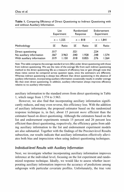
auxiliary information to the standard errors from direct questioning in Table
1, which range from 1.574 to 3.963.
However, we also find that incorporating auxiliary information signifi-
cantly reduces, and may even reverse, this efficiency loss. With the addition
of auxiliary information, the proposed estimator based on the randomized
response technique is, in fact, about 15 percent more efficient than the
estimator based on direct questioning. Although the estimators based on the
list and endorsement experiments remain 15 percent and 26 percent less
efficient than direct questioning, respectively, the efficiency gains from add-
ing auxiliary information to the list and endorsement experiment models
are also substantial. Together with the findings of the Precinct-level Results
subsection, our results indicate that auxiliary information effectively allevi-
ates both bias and imprecision when using indirect questioning techniques.
Individual-level Results with Auxiliary Information
Next, we investigate whether incorporating auxiliary information improves
inference at the individual level, focusing on the list experiment and rando-
mized response technique. Ideally, we would like to assess whether incor-
porating auxiliary information improves the accuracy of predictions among
subgroups with particular covariate profiles. Unfortunately, the true vote
Table 1. Comparing Efficiency of Direct Questioning to Indirect Questioning withand without Auxiliary Information.
Methodology
ListExperiment
RandomizedResponse
EndorsementExperiment
n ¼ 1,325 n ¼ 818 n ¼ 1,841
SE Ratio SE Ratio SE Ratio
Direct questioning .017 .021 .224No auxiliary information .067 3.963 .040 1.928 .348 1.574With auxiliary information .019 1.150 .018 0.855 .276 1.264
Note: This table compares the average standard errors (SEs) under direct questioning with thosefrom indirect questioning. We use the ratio of the average SEs from each indirect questioningmethod to the direct questioning SEs as a measure of efficiency loss or gain (though note thatthese ratios cannot be compared across question types, since the estimators are different).Whereas indirect questioning is always less efficient than direct questioning in the absence ofauxiliary information, incorporating auxiliary information occasionally results in smaller averageSEs than even direct questioning. In addition, auxiliary information always improves efficiencyrelative to no auxiliary information.
Chou et al. 19

choice for any specific individual is unavailable from official records. Thus,
we compare the association between individual-level covariates and
responses to the sensitive item across the methods.
Following Rosenfeld et al. (2016), our analysis focuses on support for the
personhood referendum by gender, party identification, and educational
level. We conduct a multiple regression analysis using the GMM approach
detailed in the second section. Given the goal of our analysis, the specifica-
tions include a larger set of survey-measured covariates including gender,
party identification, education, age, and age squared. We use survey-
measured covariates for this analysis to minimize problems of missingness
in the voter-file covariates. These specifications thus differ slightly from the
specifications used to produce the poststratified estimates in Figure 1, which
included only voter-file covariates compatible with available population data
to produce regression-adjusted population estimates.
Figure 2 presents a comparison of the estimated share of the sensitive trait
across several subgroups of the population. We omit the results for age as
neither of the two age variables was statistically significant in any of the
models. For each category of respondents, the figure presents four estimates:
open circles denote estimates from the list experiment without auxiliary
0.0
0.1
0.2
0.3
0.4
0.5
0.6
0.7
0.8
0.9
1.0
Estim
ated
pro
porti
on o
f 'no
' vot
es o
n Pe
rson
hood Gender Party Education
Male Female Republican Democrat No Higher Higher
List ExperimentList Experiment with Auxiliary InformationRandomized ResponseRandomized Response with Auxiliary Information
Figure 2. Comparison of responses across subgroups based on models with individual-level covariates. This figure compares the estimated prevalence of the sensitive trait,voting against the personhood referendum, across several categories of respondentsbased on gender, party identification, and educational level. The results in this figure arebased on survey-measured covariates. For each subgroup, the figure presents fourestimates using the list experiment, the list experiment with auxiliary information, therandomized response technique, and the randomized response technique with auxiliaryinformation. The vertical bars indicate 95 percent confidence intervals.
20 Sociological Methods & Research XX(X)

information; closed circles denote estimates from the list experiment with
auxiliary information; open squares represent randomized response estimates
without auxiliary information; and closed squares represent randomized
response estimates with auxiliary information. As before, the added auxiliary
information consists of county-level vote shares.
We begin by noting that the estimates based on auxiliary information are more
consistent across methods than the estimates without it. They are also generally
closer to the statewide mean. The effect of incorporating auxiliary information is
especially pronounced for the list experiment (i.e., the open and closed circles in
Figure 2). Incorporating auxiliary information greatly reduces the variance of the
predictions from the list experiment and brings them closer to the estimates from
randomized response technique. Given that the list experiment was found by
Rosenfeld et al. (2016) to yield the most biased estimates in previous analyses of
these data, we interpret the fact that the auxiliary information brings the list experi-
ment estimates into greater alignment with the randomized response estimates as an
encouraging sign that our approach is potentially effective for reducing bias.
Additionally, by comparing the lines (representing 95 percent confidence
intervals) extending from the open and closed shapes in Figure 2, we can see that
the auxiliary information increases the precision of estimates and alters our sta-
tistical inference for partisan affiliation and education. Whereas the list experi-
ment did not initially show statistically significant differences in support between
Democrats and Republicans, incorporating the county-level results reveals sta-
tistically significant differences in partisanship. Additionally, while neither the
list experiment nor the randomized response technique showed statistically sig-
nificant differences in education, incorporating auxiliary information indicates
that voters with higher education were significantly more likely to vote against the
personhood amendment relative to those without higher education. We view this
as an encouraging sign given that partisanship and education have been found to
be substantively important and strong predictors of abortion attitudes in research
based on efficient but potentially biased direct questioning (e.g., Adams 1997).7
By improving the efficiency of indirect questioning, our approach enables
researchers to balance the need for accurate estimates of sensitive traits with the
need to examine individual-level heterogeneity efficiently.
Specification Test
Lastly, we perform a specification test for the list experiment and rando-
mized response technique to test the fundamental assumption of our
approach to the list experiment and randomized response technique, which
is that the model parameters are constant across counties (or, more
Chou et al. 21

generally, across the groups corresponding by the auxiliary constraints).
This assumption can be tested using the standard overidentification test,
which gauges whether the observed data are consistent with the orthogon-
ality conditions used in equation (3). Given that the validity of indirect
questioning techniques is the subject of growing literature, which has at
times yielded conflicting results, we strongly recommend that researchers
conduct the overidentification test, which provides a principled means of
deciding whether large deviations from the population moments are due to
sampling variability, model misspecification, or residual bias in indirect
questioning. Table 2 presents the coefficient estimates, standard errors,
and results of the overidentification test for the list experiment and the
randomized response technique used to produce the poststratified esti-
mates presented in Figure 1, first without and then with the auxiliary
county-level information.
We find that incorporating auxiliary information reduces the size of the
standard errors for virtually all coefficients in both the list experiment and the
Table 2. Specification Test with and without Auxiliary Information.
Coefficient
List Experiment Randomized Response
No AuxiliaryInformation
With AuxiliaryInformation
No auxiliaryInformation
With AuxiliaryInformation
Estimates SE Estimates SE Estimates SE Estimates SE
(Intercept) �.58 .81 �1.85 .46 �0.36 .61 �7.37 .44Democrat .81 .70 �1.07 .64 �0.54 .57 �6.90 .64Republican .57 .55 1.60 .50 1.00 .31 0.99 .28Male .57 .51 0.84 .51 0.22 .30 0.52 .29Missing age .31 .77 0.25 .17 �0.71 .58 5.99 .34Aged 55 and over 0.01 .72 7.11 .48Overidentification
test145.84 (<0.01) 12.35 (0.87)
Note: This table shows the coefficients, standard errors (SEs), and results of the overidentifica-tion test for the list experiment and randomized response models with individual covariates.These covariates correspond to the voter-file covariates used to produce the poststratifiedestimates in Figure 1. Incorporating auxiliary information in the form of 19 county-level electionresults reduces the SE of the coefficient estimates. The overidentification test gauges whetherthe moment conditions used in the generalized method of moments estimation are consistentwith the observed data. Low p values of the overidentification test statistic (reported in par-entheses) indicate that the model is inconsistent with the data. We find that the momentconditions associated with our list experiment model are inconsistent with the data (p < :01).
22 Sociological Methods & Research XX(X)
randomized response technique. This increased efficiency is due to the addi-
tional orthogonality conditions implied by our auxiliary information. How-
ever, the large test statistic (and its corresponding small p value shown in
parentheses) from the overidentification test for the list experiment indicates
that the moment conditions in equation (3) are inconsistent with the observed
data. While this indicates that at least some aspects of our model for the list
experiment are invalid, the finding is consistent with the analysis of these
data by Rosenfeld et al. (2016), which shows that the list experiment yielded
substantially more biased estimates relative to the randomized response
technique and the endorsement experiment. On the other hand, the over-
identification test for the randomized response technique implies that
the model’s overidentifying restrictions are consistent with the observed data
(p ¼ .87). We therefore conclude that our assumption that the model and set
of parameters are constant across counties is reasonable given the data.
Simulation Studies
In this section, we conduct two simulation studies to explore the conditions
under which our method is effective for improving inference for multivariate
relationships. We focus on the proposed estimators for the list experiment
and randomized response technique, as our approach for the endorsement
experiment is more appropriate for improving predictions in hierarchically
structured data rather than improving multivariate inference for individual-
level covariates.
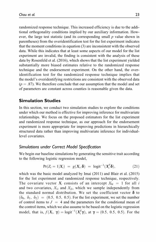
Simulations under Correct Model Specification
We begin our baseline simulations by generating the sensitive trait according
to the following logistic regression model,
PrðZi ¼ 1jXiÞ ¼ gðXi; δÞ ¼ logit�1ðXTi δÞ; ð21Þ
which was the basic model analyzed by Imai (2011) and Blair et al. (2015)
for the list experiment and randomized response technique, respectively.
The covariate vector Xi consists of an intercept X0i ¼ 1 for all i
and two covariates, X1i and X2i, which we sample independently from
the standard normal distribution. We set the coefficient vector δ to
ðd0; d1; d2Þ ¼ ð0:5; 0:5; 0:5Þ. For the list experiment, we set the number
of control items to J ¼ 4 and the parameters for the conditional mean of
the control items, which we also assume to be based on the logistic regression
model, that is, f ðXi; γÞ ¼ logit�1ðXTi γÞ, at γ ¼ ð0:5; 0:5; 0:5Þ. For the
Chou et al. 23

randomized response technique, we use the forced response design with the
probability of a forced yes set to p1 ¼ :5 while assuming the same logistic
regression model for gðXi; δÞ applied to the list experiment.
We then assess the performance of our estimators by varying the correla-
tion between the group assignment and the covariates, where we simulate
K ¼ 5 groups in various ways as described below. In all cases, we begin
with a population consisting of 10 million units. This enables us to approx-
imate the group-specific moments h precisely, as there is no closed form
expression for h. To construct the group labels Gi, we first generate a con-
tinuous group assignment variable G�i together with X1 and X2 from a multi-
variate normal distribution where each random variable has a unit variance.
We vary the correlations among these three variables in order to simulate
different degrees of segregation, that is, the degree to which respondents with
different covariate values are separated across groups such as counties or
precincts. Lastly, we generate the group labels Gi by assigning labels to cut
points as in an ordinal probit model, with the cut points chosen to equalize the
number of individuals in each group.
We focus on the following four scenarios, in which the researcher knows
the prevalence of the sensitive trait in all K ¼ 5 groups, that is,
h ¼ ðh1; h2; h3; h4; h5Þ:
1. In the no segregation scenario, both X1 and X2 are independent of
each other, and they are uncorrelated with G�i . This scenario is shown
in the first row of Figure 3, which depicts the identical distributions of
X1 across the five groups. In this example, the group-specific
moments hk are all equal in expectation to the population mean of h.
2. In the segregation on X1 scenario, both X1 and X2 are independently
drawn. However, the first covariate X1 is correlated with the group
assignment variable G�i at .5. This scenario is shown in the second
panel of Figure 3. In this example, X1i is not uniformly distributed
across groups. As a result, there exists a correlation between the
group-specific moments h and the group labels.
3. In the segregation on X1 and X2 scenario, X1 and X2 remain inde-
pendent. However, each is correlated with the group assignment
variable G�i at .5.
4. In the X1 and X2 correlated scenario, X1 and X2 are mutually correlated
at .5 and correlated with the group assignment variable G�i at 0:5.
Once we simulate these varying levels of segregation, we proceed to
estimate the parameters of interest d for each indirect questioning
24 Sociological Methods & Research XX(X)

technique with and without auxiliary information. Our results are summar-
ized in Figures 4 and 5 for the list experiment and the randomized response
technique, respectively. The three columns in each figure correspond to
the coefficient for the intercept d0 and the coefficients of the two covari-
ates, X1 and X2, in the parametric model for the sensitive item, d1 and d2,
while the rows report the absolute bias, RMSE, and coverage of the 95
percent confidence intervals. We evaluate the empirical performance of
our estimators over 5,000 Monte Carlo simulations at sample sizes ranging
from 1,000 to 10,000.
In Figure 4, the standard list experiment estimator without auxiliary
information is represented by open lines and solid circles. Comparing the
standard estimator to the other four lines, we find that the auxiliary infor-
mation results in lower levels of bias across all four scenarios, although
these gains converge to zero as the sample size increases. This finding,
which is indicated by the downward sloping lines in the first row of Figure
4, is due to the fact that the standard estimator for the list experiment is also
consistent despite its inefficiency.
On the other hand, the improvements in the RMSE are confined to the
scenarios when covariates are correlated with the group assignment, which
−2−1
01
2
Group 1 Group 2 Group 3 Group 4 Group 5
−2−1
01
2
X1X1
No Segregation on X1
Segregation on X1
Figure 3. No segregation versus segregation scenarios. This figure illustrates thesimulated distribution of X1 for the no segregation and segregation on X1 scenarios inour simulation study. The solid lines correspond to the mean of X1i in each group,while the dashed lines correspond to the overall mean of X1i, m1 ¼ 0.
Chou et al. 25

results in a nonuniform distribution of the covariates across groups. This can
be seen by focusing on the triangles in the second row of Figure 4, which
represent the segregation on X1 (open triangles with solid lines) and
δ0
Sample Size
Bias
−0.0
10
0.01
0.02
1000 2500 10000
δ1
Sample Size
Bias
−0.0
10
0.01
0.02
1000 2500 10000
δ2
Sample Size
Bias
−0.0
10
0.01
0.02
1000 2500 10000
No aux. infoNo segregationSegregation on X1Segregation on X1, X2X1, X2 correlated
0.00
0.05
0.10
0.15
0.20
δ0
Sample Size
RM
SE
1000 2500 10000
0.00
0.05
0.10
0.15
0.20
δ1
Sample Size
RM
SE
1000 2500 10000
0.00
0.05
0.10
0.15
0.20
δ2
Sample Size
RM
SE
1000 2500 10000
No aux. infoNo segregationSegregation on X1Segregation on X1, X2X1, X2 correlated
0.90
0.92
0.94
0.96
0.98
1.00
δ0
Sample Size
Cov
erag
e
1000 2500 10000
0.90
0.92
0.94
0.96
0.98
1.00
δ1
Sample Size
Cov
erag
e
1000 2500 10000
0.90
0.92
0.94
0.96
0.98
1.00
δ2
Sample Size
Cov
erag
e
1000 2500 10000
No aux. infoNo segregationSegregation on X1Segregation on X1, X2X1, X2 correlated
Figure 4. Empirical performance of the proposed estimator for the list experimentwith auxiliary information. This figure illustrates the bias, root mean square error, andcoverage of 95 percent confidence intervals for the nonlinear least squares estimatorof Imai (2011), with and without auxiliary information, over 5,000 Monte Carlosimulations. The continuously updating generalized method of moments estimator isused for all simulations. Each line corresponds to a different scenario: open circles andsolid lines correspond to the baseline estimator with no auxiliary information; closedcircles and dashed lines correspond to the no segregation scenario; open trianglesand solid lines correspond to the segregation on X1 scenario; closed triangles anddashed lines correspond to segregation on X1 and X2 with uncorrelated covariates;and crosses and solid lines correspond to segregation on X1 and X2 with correlatedcovariates.
26 Sociological Methods & Research XX(X)

segregation on X1 and X2 scenarios (closed triangles with dashed lines). The
auxiliary information does not result in lower RMSE for 1 and 2 unless there
is segregation on X1 and X2, respectively. Thus, the auxiliary information is
helpful when the covariates are correlated with the group labels.
●●
●
δ0
Sample Size
Bias
−0.0
10
0.01
0.02
1000 2500 10000
● ● ●
●
●●
δ1
Sample Size
Bias
−0.0
10
0.01
0.02
1000 2500 10000
●
● ●
●
●
●
δ2
Sample Size
Bias
−0.0
10
0.01
0.02
1000 2500 10000
●● ●
●
●
No aux. infoNo segregationSegregation on X1Segregation on X1, X2X1, X2 correlated
●
●
●
0.00
0.05
0.10
0.15
0.20
δ0
Sample Size
RM
SE
1000 2500 10000
●
●
●
●
●
●
0.00
0.05
0.10
0.15
0.20
δ1
Sample Size
RM
SE
1000 2500 10000
●
●
●
●
●
●0.
000.
050.
100.
150.
20
δ2
Sample Size
RM
SE
1000 2500 10000
●
●
●
●
●
No aux. infoNo segregationSegregation on X1Segregation on X1, X2X1, X2 correlated
●●
●
0.90
0.92
0.94
0.96
0.98
1.00
δ0
Sample Size
Cov
erag
e
1000 2500 10000
● ● ●
●●
●
0.90
0.92
0.94
0.96
0.98
1.00
δ1
Sample Size
Cov
erag
e
1000 2500 10000
●
●●
●●
●
0.90
0.92
0.94
0.96
0.98
1.00
δ2
Sample Size
Cov
erag
e
1000 2500 10000
●●
●
●
●
No aux. infoNo segregationSegregation on X1Segregation on X1, X2X1, X2 correlated
Figure 5. Empirical performance of the proposed estimator for the randomizedresponse technique. This figure illustrates the bias, root mean square error, andcoverage of 95 percent confidence intervals for the likelihood estimator of Blair et al.(2015), with and without auxiliary information, over 5,000 Monte Carlo simulations.The continuously updating generalized method of moments estimator is used for allsimulations. Each line corresponds to a different scenario: open circles and solid linescorrespond to the baseline estimator with no auxiliary information; closed circles anddashed lines correspond to the no segregation scenario; open triangles and solid linescorrespond to the segregation on X1 scenario; closed triangles and dashed linescorrespond to segregation on X1 and X2 with uncorrelated covariates; and crossesand solid lines correspond to segregation on X1 and X2 with correlated covariates.
Chou et al. 27

Even when there is segregation on both covariates, however, the improve-
ments in the RMSE are much smaller when X1 and X2 are correlated, as the
two variables contain some redundant information. This is represented by the
solid lines with cross marks in the second row of Figure 4, which lie close to
the RMSE of the estimator without auxiliary information. Lastly, the third
row of Figure 4 shows that the estimated 95 percent confidence intervals
have coverage rates close to their nominal levels, although the coverage rates
are near 90 percent when there is no segregation (dashed lines with closed
circles) and when the sample size is small.
Turning to the randomized response technique in Figure 5, we find that,
although the improvements in bias are smaller due to the greater overall
efficiency of the randomized response technique, the improvements in
RMSE follow a similar pattern. This can be seen by focusing on the trian-
gles in the second row of Figure 5, which again correspond to scenarios
with segregation on X1 only (open triangles with solid lines) and with
segregation on both X1 and X2 (closed triangles with dashed lines). The
auxiliary information results in more efficient estimates of d^1 and d^2 only
when there exists segregation on X1 and X2, respectively, and when the
covariates are not highly correlated. These improvements remain substan-
tial even as the sample size becomes very large, as can be seen in the second
row of Figure 5. Finally, the coverage rates of the estimated 95 percent
confidence intervals are also close to or above their nominal levels, as can
be seen in the third row of Figure 5.
Taken together, Figures 4 and 5 indicate that the effectiveness of our
approach for improving multivariate inference hinges on the extent of seg-
regation. When there is no segregation on the covariates, the auxiliary infor-
mation only improves inference for the intercept and does not result in more
efficient estimates of the other coefficients. Conversely, when covariates are
unevenly distributed across groups, auxiliary information can increase effi-
ciency across different sample sizes. Furthermore, these improvements are
greater when covariates are less correlated.
Comparison with Direct Questioning
We next examine the efficiency of our proposed estimators relative to direct
questioning. To do this, we use the same simulation setting as above and
assume that the sensitive trait is truthfully observed for each individual. We
estimate the logistic regression model given in equation (21) using the
observed sensitive trait and compare the size of the resulting standard errors
with those from the conventional estimators for the list experiment and
28 Sociological Methods & Research XX(X)

randomized response with and without the auxiliary information. Table 3
reports the findings from 5,000 Monte Carlo simulations for each of our four
scenarios described above. The table shows the standard errors along with the
ratio of the indirect questioning standard errors to the direct questioning
standard errors. Ratios greater (less) than 1 indicate that the estimator is less
(more) efficient than direct questioning. We limit the presentation of results
to sample sizes of 2,500 for clarity.
We find that indirect questioning typically results in a large efficiency
loss when no auxiliary information is available as shown in the previous
simulation studies (e.g., Blair et al. 2015; Imai 2011). This can be seen in
the ratios of the standard errors without auxiliary information to the
standard errors from direct questioning in Table 3, which range from
1.64 to 1.95. In other words, the standard errors from the conventional
indirect questioning estimators are nearly twice as large as the standard
errors that we would obtain assuming that the sensitive trait were truth-
fully observed.
However, we also find that incorporating auxiliary information can sig-
nificantly mitigate and even reverse this efficiency loss. This can be seen
especially in the ratios for the intercept d0 in Table 3, which range from 0.25
to 0.86. These ratios indicate that the estimates of the intercept using indirect
questioning and auxiliary information are more efficient than even direct
questioning. On the other hand, the ratios for the coefficients are greater
than 1 except for the list experiment when there is segregation on X1 across
groups, meaning that auxiliary information does not fully offset the effi-
ciency loss for these parameters. Nevertheless, auxiliary information always
improves efficiency relative to indirect questioning without auxiliary infor-
mation. Setting aside the intercept, we find that auxiliary information allows
us to recoup an average of 43 percent of the direct questioning standard error
for the list experiment and an average of 16 percent for the randomized
response technique. These gains are larger when the covariates are segre-
gated and when they are less correlated.
Simulations under Model Misspecification
We also conduct a separate simulation study to explore the benefits of aux-
iliary information under model misspecification, a routine concern for
applied researchers. We begin by generating the sensitive trait according
to the following logistic regression model:
PrðZi ¼ 1jXiÞ ¼ logit�1ð�1 þ 0:5X1i þ 0:5X2i þ 0:5X 22iÞ; ð22Þ
Chou et al. 29

Tab
le3.
Com
par
ing
Effic
iency
ofD
irec
tQ
ues
tionin
gto
Indir
ect
Ques
tionin
gw
ith
and
without
Auxili
ary
Info
rmat
ion.
Scen
ario
List
Exper
imen
tR
andom
ized
Res
ponse
d 0d 1
d 2d 0
d 1d 2
SER
atio
SER
atio
SER
atio
SER
atio
SER
atio
SER
atio
No
segr
egat
ion
Dir
ect
ques
tionin
g.0
4.0
5.0
5.0
4.0
5.0
5N
oau
xili
ary
info
rmat
ion
.08
1.9
0.0
91.9
3.0
91.9
3.0
71.6
4.0
81.6
9.0
81.6
9W
ith
auxili
ary
info
rmat
ion
.02
0.4
3.0
91.8
8.0
91.8
8.0
40.8
6.0
81.6
7.0
81.6
7Se
greg
atio
non
X1
Dir
ect
ques
tionin
g.0
4.0
5.0
5.0
4.0
5.0
5N
oau
xili
ary
info
rmat
ion
.08
1.9
0.0
91.9
3.0
91.9
3.0
71.6
4.0
81.6
9.0
81.6
9W
ith
auxili
ary
info
rmat
ion
.02
0.3
7.0
30.6
7.0
91.8
8.0
40.8
6.0
61.3
3.0
81.6
7Se
greg
atio
non
X1
and
X2
Dir
ect
ques
tionin
g.0
4.0
5.0
5.0
4.0
5.0
5N
oau
xili
ary
info
rmat
ion
.08
1.9
0.0
91.9
3.0
91.9
3.0
71.6
4.0
81.6
9.0
81.6
9W
ith
auxili
ary
info
rmat
ion
.01
0.2
5.0
61.2
5.0
61.2
6.0
40.8
5.0
61.4
0.0
61.3
9X
1an
dX
2co
rrel
ated
Dir
ect
ques
tionin
g.0
4.0
5.0
5.0
4.0
5.0
5N
oau
xili
ary
info
rmat
ion
.09
1.9
3.1
01.9
5.1
01.9
5.0
71.6
5.0
91.7
0.0
91.6
9W
ith
auxili
ary
info
rmat
ion
.02
0.3
4.0
81.5
9.0
81.5
9.0
40.8
6.0
81.5
6.0
81.5
6
Not
e:T
his
table
com
par
esth
est
andar
der
rors
(SEs)
under
dir
ect
ques
tionin
gw
ith
those
from
indir
ect
ques
tionin
gw
hen
the
sensi
tive
trai
tis
gener
ated
asin
Figu
re4.W
euse
the
ratio
oft
he
estim
ated
SEs
toth
edir
ect
ques
tionin
gSE
sas
am
easu
reoft
he
effic
iency
loss
or
gain
.In
contr
ast
toth
eco
nve
ntional
indir
ect
ques
tionin
gSE
s,w
hic
har
eal
way
sle
ssef
ficie
ntth
andir
ectques
tionin
g,au
xili
ary
info
rmat
ion
occ
asio
nal
lyre
sults
insm
alle
rSE
sth
anev
endir
ectques
tionin
g.W
eal
sofin
dth
atau
xili
ary
info
rmat
ion
alw
ays
impro
ves
effic
iency
rela
tive
tono
auxili
ary
info
rmat
ion.
30

where we slightly modify the value of δ to balance the number of units with
and without the sensitive trait. To generate X1, we simulate a latent variable X �1from the standard normal distribution and set X1 ¼ 1 if X �1 > 0 and 0
otherwise. Discretizing X1 allows us to examine the effect of the auxiliary
information on predictions for subpopulations defined by X1 2 f0; 1g. We
then generate X2 from the standard normal distribution such that X �1 and X2 are
correlated at .5. Lastly, we generate K ¼ 5 groups using a group assignment
variable that is correlated with X �1 at .5 and selecting cut points as before.
After simulating our initial population, we generate predictions for the
subgroups defined by X1 using a misspecified model that omits the squared
term from equation (22). We then examine whether the auxiliary information
is able to improve inference for the coefficient of X1 in spite of the bias
induced by the misspecification in the presence of correlation between X1
and X2. Figure 6 reports the results from 5,000 Monte Carlo simulations for
both indirect questioning techniques at sample sizes ranging from 1,000 to
10,000. In the first column, we compare the true prevalence of the sensitive
trait for the two groups defined by the value of X1 to the predicted prevalence
with and without auxiliary information. We find that the auxiliary informa-
tion typically reduces both the variance and the bias of the predictions. This
is represented by the shorter length of the dashed lines, which represent the
range of estimates with auxiliary information, and by the closeness of the
mean predictions to the population averages.
The second column of Figure 6 shows the RMSE of the predictions for
sample sizes ranging from 1,000 to 10,000. Although the RMSE does not
converge to 0 due to the model misspecification, we find that the auxiliary
information results in more precise estimates of the sensitive trait. This is true
even for large sample sizes, as can be seen by the RMSE for sample sizes of
10,000. The gains from the auxiliary information are especially large for the
list experiment and for smaller sample sizes. These results suggest that
auxiliary information can be useful for making more robust and precise
predictions even when a misspecified model is used, as is often the case in
applied research.
Concluding Remarks
Despite their importance in social science research, sensitive topics such as
vote choice, health, illicit behavior, and contact with the criminal justice
system continue to present serious methodological challenges. Social desir-
ability bias and high rates of item nonresponse make it especially difficult to
measure the prevalence of sensitive attitudes and behaviors. Indirect
Chou et al. 31

questioning techniques hold considerable promise for alleviating these
sources of bias. However, they also entail a major loss of efficiency that can
make multivariate inference and prediction for small groups impossible.
In this article, we present a method for improving statistical analysis of
indirect questioning techniques by exploiting auxiliary information about the
population under study. Such information may be available from official
0.4
0.5
0.6
0.7
0.8
0.9
1.0
Predictions under Model Misspecification
X1
Prev
alen
ce o
f Sen
sitiv
e Tr
ait
0 1
Population MeanX1 = 0 without Auxiliary InformationX1 = 1 without Auxiliary InformationX1 = 0 with Auxiliary InformationX1 = 1 with Auxiliary Information
0.00
0.01
0.02
0.03
0.04
0.05
0.06
Root Mean Squared Error
Sample SizeR
MSE
1000 2500 10000
0.4
0.5
0.6
0.7
0.8
0.9
1.0
X1
Prev
alen
ce o
f Sen
sitiv
e Tr
ait
0 1
Population MeanX1 = 0X1 = 1X1 = 0 w/ Auxiliary InformationX1 = 1 w/ Auxiliary Information
0.00
0.01
0.02
0.03
0.04
0.05
0.06
Sample Size
RM
SE
1000 2500 10000
Lis
tE
xper
imen
tR
and
om
ized
Res
po
nse
Figure 6. Comparing predictions under model misspecification with and withoutauxiliary information. This figure summarizes the results of 5,000 Monte Carlosimulations, in which predictions were generated using a misspecified model for twosubgroups defined by a binary covariate X1. Auxiliary information refers to knowl-edge of the prevalence of the sensitive trait in five groups, over which X1 is unevenlydistributed. The vertical bars correspond to the difference between the 2.5 percentand 97.5 percent quantiles across all simulations. Auxiliary information reduces theroot mean square error of the predictions by up to 50 percent. The gains fromauxiliary information are largest for the list experiment and for smaller sample sizes.
32 Sociological Methods & Research XX(X)

sources, administrative records, or expert evaluations. In this study, we took
advantage of official voting data—a source of auxiliary information that may
be relevant for a range of research questions on sensitive topics including
turnout, nationalist party support, and vote choice on other referendums
involving sensitive social issues. We demonstrate that aggregate-level auxili-
ary information can improve multivariate inference and prediction when ana-
lyzing three popular indirect questioning techniques: the list experiment,
randomized response technique, and endorsement experiment. Empirical and
simulation studies find that such aggregate information can increase the effi-
ciency, reduce the bias due to model misspecification, and improve the pre-
dictive accuracy of quantities at a lower level of aggregation. In some cases,
the addition of auxiliary information completely recovers the efficiency loss
relative to direct questioning. Finally, we enable researchers to implement the
proposed methods by making them available through open-source software.
Authors’ Note
The methods described in this article can be implemented via the open-source
statistical software, endorse: R Package for Analyzing Endorsement Experiments,
list: Statistical Methods for the Item Count Technique and List Experiment, and rr:
Statistical Methods for the randomized response technique, all of which are
available through the Comprehensive R Archive Network (http://cran.r-projec
t.org/http://cran.r-project.org/). The replication archive for this article is available
as Chou, Winston; Imai, Kosuke; and Rosenfeld, Bryn, 2017, “Replication Data for:
Sensitive Survey Questions with Auxiliary Information,” doi:10.7910/DVN/
4FEJZ3, Harvard Dataverse.
Acknowledgment
We thank Ryan Bakker for useful comments and Grame Blair and Yuki Shiraito for
answering our questions.
Declaration of Conflicting Interests
The author(s) declared no potential conflicts of interest with respect to the research,
authorship, and/or publication of this article.
Funding
The author(s) received no financial support for the research, authorship, and/or pub-
lication of this article.
Supplemental Material
Supplementary material for this article is available online.
Chou et al. 33
Notes
1. Of course, the estimators based on direct questioning can also be made more
efficient by incorporating auxiliary information, but our comparison is based on
direct questioning without such information.
2. In principle, a group G can be any set of respondents associated with a known
population moment. For example, Aronow et al. (2015) propose to combine
direct questioning and list experiment by assuming that respondents who answer
affirmatively under direct questioning have the sensitive trait with probability 1.
Our framework can accommodate this “no false confessions” assumption by
letting Gi ¼ 1 represent the affirmative answer to the direct question and
setting h1 ¼ 1. In fact, it is even possible to incorporate both the true preva-
lence at an aggregate level and the no false confessions assumption based on
direct questioning at the same time.
3. See also the Placebo Test I of Aronow et al. (2015).
4. This design is unusual in that it does not obscure the negative answer to this sensitive
question, which in this context may be seen as a socially undesirable answer.
5. Because the sample size varies across indirect methods, it is not straightforward to
assess these methods’ efficiency relative to each another using the results below.
Rather, the results in this section highlight the efficiency gained or lost by these
indirect methods relative to direct questioning.
6. Note that one cannot compare the results across questioning techniques since
different estimators are used.
7. The Mississippi validation study included a direct questioning sample, and previ-
ous analyses by Rosenfeld et al. (2016) showed statistically significant differences
in partisanship and education based on this sample. However, the estimates from
direct questioning were highly biased, with all groups avowing significantly
greater support for the personhood amendment than the statewide election result.
In Figure S8 of Online Appendix B, we replicate their findings and compare them
with those based on our methods using the same sample sizes.
References
Adams, G. D. 1997. “Abortion: Evidence of an Issue Evolution.” American Journal of
Political Science 41:718-37.
Aronow, P. M., A. Coppock, F. W. Crawford, and D. P. Green. 2015. “Combining
List Experiment and Direct Question Estimates of Sensitive Behavior Prevalence.”
Journal of Survey Statistics and Methodology 3:43-66.
Blair, G. and K. Imai. 2012. “Statistical Analysis of List Experiments.” Political
Analysis 20:47-77.
34 Sociological Methods & Research XX(X)

Blair, G. and K. Imai. 2016. “List: Statistical Methods for the Item Count Technique
and List Experiment.” Comprehensive R Archive Network (CRAN). Version 8.3.
Retrieved September 26, 2017. (http://CRAN.R-project.org/package¼list).
Blair, G., K. Imai, and J. Lyall. 2014. “Comparing and Combining List and Endorse-
ment Experiments: Evidence from Afghanistan.” American Journal of Political
Science 58:1043-63.
Blair, G., K. Imai, and Y.-Y. Zhou. 2015. “Design and Analysis of Randomized
Response Technique.” Journal of the American Statistical Association 110:
1304-19.
Blair, G., Y.-Y. Zhou, and K. Imai. 2016. “rr: Statistical Methods for the Randomized
Response.” Comprehensive R Archive Network (CRAN). Version 1.4. Retrieved
September 26, 2017. (http://CRAN.R-project.org/package¼rr).
Bullock, W., K. Imai, and J. N. Shapiro. 2011. “Statistical Analysis of Endorsement
Experiments: Measuring Support for Militant Groups in Pakistan.” Political Anal-
ysis 19:363-84.
Coutts, E. and B. Jann. 2011. “Sensitive Questions in Online Surveys: Experimental
Results for the Randomized Response Technique (RRT) and the Unmatched
Count Technique (UCT).” Sociological Methods & Research 40:169-93.
Cross, P. J. and C. F. Manski. 2002. “Regressions, Short and Long.” Econometrica
70:357-68.
Duncan, O. D. and B. Davis. 1953. “An Alternative to Ecological Correlation.”
American Sociological Review 18:665-66.
Gingerich, D. W. 2010. “Understanding Off-the-books Politics: Conducting Inference
on the Determinants of Sensitive Behavior with Randomized Response Surveys.”
Political Analysis 18:349-80.
Gonzalez-Ocantos, E., C. K. de Jonge, C. Melendez, J. Osorio, and D. W. Nickerson.
2012. “Vote Buying and Social Desirability Bias: Experimental Evidence from
Nicaragua.” American Journal of Political Science 56:202-17.
Greiner, D. J. and K. M. Quinn. 2010. “Exit Polling and Racial Bloc Voting: Com-
bining Individual Level and Ecological Data.” Annals of Applied Statistics 4:
1774-96.
Handcock, M. S., M. S. Rendall, and J. E. Cheadle. 2005. “Improved Regression
Estimation of a Multivariate Relationship with Population Data on the Bivariate
Relationship.” Sociological Methodology 35:291-334.
Hansen, L. P. 1982. “Large Sample Properties of Generalized Method of Moments
Estimators.” Econometrica 50:1029-54.
Hansen, L. P., J. Heaton, and A. Yaron. 1996. “Finite-sample Properties of Some Alter-
native GMM Estimators.” Journal of Business & Economic Statistics 14:262-80.
Hanson, T. E., A. J. Branscum, and W. O. Johnson. 2014. “Informative g-priors for
Logistic Regression.” Bayesian Analysis 9:597-612.
Chou et al. 35
Hellerstein, J. K. and G. W. Imbens. 1999. “Imposing Moment Restrictions from
Auxiliary Data by Weighting.” Review of Economics and Statistics 81:1-14.
Imai, K. 2011. “Multivariate Regression Analysis for the Item Count Technique.”
Journal of the American Statistical Association 106:407-16.
Imai, K. and K. Khanna. 2016. “Improving Ecological Inference by Predicting Indi-
vidual Ethnicity from Voter Registration Record.” Political Analysis 24:263-72.
Imbens, G. and T. Lancaster. 1994. “Combining Micro and Macro Data in Micro-
econometric Models.” The Review of Economic Studies 61:655-80.
Jackson, C., N. Best, and S. Richardson. 2008. “Hierarchical Related Regression for
Combining Aggregate and Individual Data in Studies of Socio-economic Disease
Risk Factors.” Journal of the Royal Statistical Society: Series A (Statistics in
Society) 171:159-78.
Janus, A. L. 2010. “The Influence of Social Desirability Pressures on Expressed
Immigration Attitudes.” Social Science Quarterly 91:928-46.
Karp, J. A. and D. Brockington. 2005. “Social Desirability and Response Validity: A
Comparative Analysis of Overreporting Voter Turnout in Five Countries.”
Journal of Politics 67:825-40.
Kim, C. and C. R. Tamborini. 2014. “Response Error in Earnings: An Analysis of the
Survey of Income and Program Participation Matched with Administrative Data.”
Sociological Methods & Research 43:39-72.
Kling, J. R., J. Ludwig, and L. F. Katz. 2005. “Neighborhood Effects on Crime for
Female and Male Youth: Evidence from a Randomized Housing Voucher Experi-
ment.” The Quarterly Journal of Economics 120:87-130.
Krumpal, I. 2012. “Estimating the Prevalence of Xenophobia and Anti-semitism in
Germany: A Comparison of Randomized Response and Direct Questioning.”
Social Science Research 41:1387-403.
Kuklinski, J. H., M. D. Cobb, and M. Gilens. 1997. “Racial Attitudes and the “New
South.”” Journal of Politics 59:323-49.
Lyall, J., G. Blair, and K. Imai. 2013. “Explaining Support for Combatants during
Wartime: A Survey Experiment in Afghanistan.” American Political Science
Review 107:679-705.
Martin, L. M., M. Leff, N. Calonge, C. Garrett, and D. E. Nelson. 2000. “Validation
of Self-reported Chronic Conditions and Health Services in a Managed Care
Population.” American Journal of Preventive Medicine 18:215-18.
Raftery, A. E., G. H. Givens, and J. E. Zeh. 1995. “Inference from a Deterministic
Population Dynamics Model for Bowhead Whales.” Journal of the American
Statistical Association 90:402-16.
Rosenfeld, B., K. Imai, and J. Shapiro. 2016. “An Empirical Validation Study of
Popular Survey Methodologies for Sensitive Questions.” American Journal of
Political Science 60:783-802.
36 Sociological Methods & Research XX(X)

Schrapler, J.-P. 2004. “Respondent Behavior in Panel Studies: A Case Study for
Income Non-response by Means of the German Socio-economic Panel (SOEP).”
Sociological Methods & Research 33:118-56.
Shiraito, Y. and K. Imai. 2015. “Endorse: R Package for Analyzing Endorsement
Experiments.” Comprehensive R Archive Network (CRAN). Version 1.6.0.
Retrieved September 26, 2017. (http://CRAN.R-project.org/ package¼endorse).
van der Heijden, P. G., G. van Gils, J. Bouts, and J. J. Hox. 2000. “A Comparison of
Randomized Response, Computer-assisted Self-interview, and Face-to-face
Direct Questioning: Eliciting Sensitive Information in the Context of Welfare and
Unemployment Benefit.” Sociological Methods & Research 28:505-37.
Warner, S. L. 1965. “Randomized Response: A Survey Technique for Eliminating
Evasive Answer Bias.” Journal of the American Statistical Association 60:63-69.
Wolter, F. and P. Preisendorfer. 2013. “Asking Sensitive Questions: An Evaluation of
the Randomized Response Technique versus Direct Questioning Using Individual
Validation Data.” Sociological Methods & Research 42:321-53.
Wyner, G. A. 1980. “Response Errors in Self-reported Number of Arrests.” Socio-
logical Methods & Research 9:161-77.
Author Biographies
Winston Chou is a PhD candidate in the Department of Politics at Princeton Uni-
versity. He studies contemporary European politics and quantitative methodology.
Kosuke Imai is a professor in the Department of Politics and the Center for Statistics
and Machine Learning at Princeton University. He is the author of Quantitative Social
Science: An Introduction (Princeton University Press, 2017).
Bryn Rosenfeld is an assistant professor in the Department of Political Science at the
University of Southern California. Her methodological research interests include
survey methods for sensitive subjects and rare political behaviors.
Chou et al. 37
Top Related