


Languages
Pages
Legal


47
Science Concept 2: The Structure and Composition of the Lunar
Interior Provide Fundamental Information on the Evolution of a
Differentiated Planetary Body
Science Concept 2: The Structure and Composition of the Lunar Interior Provide Fundamental
Information on the Evolution of a Differentiated Planetary Body
Science Goals:
a. Determine the thickness of the lunar crust (upper and lower) and characterize its lateral
variability on regional and global scales.
b. Characterize the chemical/physical stratification in the mantle, particularly the nature of the
putative 500-km discontinuity and the composition of the lower mantle.
c. Determine the size, composition, and state (solid/liquid) of the core of the Moon.
d. Characterize the thermal state of the interior and elucidate the workings of the planetary heat
engine.
INTRODUCTION
Each of the Science Goals addressed by Science Concept 2 is linked: data regarding the crust, mantle,
and core must be obtained in order to understand the thermal state of the interior and the planetary heat
engine. Much about these Science Goals is currently unknown: crustal thickness and lateral variability are
constrained by gravity and seismic models which suffer from non-uniqueness and a lack of control points;
mantle composition is ambiguously estimated from seismic velocity profiles and assumed lunar bulk
compositions; mantle structure is obtained through seismic velocity profiles, but fine-scale structure is not
resolved and any structure outside the Apollo network and below 1000 kilometers depth is unknown; the
size, composition and state of the core are obtained through models with few constraints, where the size
and state are dependent on an unknown composition, making any core characteristic estimates highly
variable; and the thermal state of the interior is constrained by heat flow measurements and characteristics
of the core, but current heat flow data are not representative of the global heat flux and core models are
non-unique. Besides elucidating the principle objectives of each Science Goal, addressing this Science
Concept will also provide data regarding formation and evolution models of the Moon (i.e., the Giant
Impact (e.g., Canup, 2004a, 2004b) and Lunar Magma Ocean (LMO; e.g., Wood et al., 1970) hypotheses,
the details of which are debated or unknown.
Understanding the formation and evolution of the Moon provides important information on planetary
and solar system evolution as a whole. The relative lack of geologic activity on the lunar surface provides
a window into processes active during early Solar System formation that have since been removed from the
Earth‘s surface. Likewise, the small size of the Moon implies a faster cooling history, preserving records
of initial composition and interior structure (NRC, 2007).
The most comprehensive hypothesis for the formation of the Moon is the collision of an object twice
the size of the Moon with the proto-Earth. Thus, the composition and thermal evolution of the Moon and
Earth were intimately linked at the beginning of the solar system (NRC, 2007). While these two bodies
have evolved independently of each other, a more complete understanding of the composition and structure
of the lunar interior will shed light on the early history of Earth.
Other studies of Science Concepts in this volume suggest landing sites and data collection that will help
address Science Concept 2. In particular, the knowledge gained by addressing Science Concept 1 will help
48
elucidate the early thermal history of the Moon (assisting Science Goal 2d). Proposed sample return for
Science Concepts 3, 5 and 6 will contribute to current knowledge of crust and mantle lithologies (assisting
Science Goals 2a, 2b). However, it should be noted that no other Science Concepts overlap with
understanding the lunar core (Science Goal 2c). The contributions of other Science Concepts to the one
considered here are outlined in more detail in each Science Goal section.
Approach
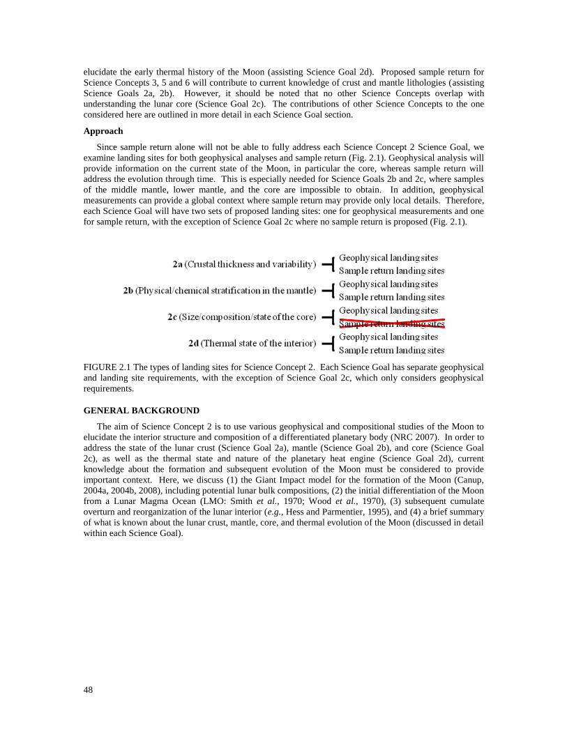
Since sample return alone will not be able to fully address each Science Concept 2 Science Goal, we
examine landing sites for both geophysical analyses and sample return (Fig. 2.1). Geophysical analysis will
provide information on the current state of the Moon, in particular the core, whereas sample return will
address the evolution through time. This is especially needed for Science Goals 2b and 2c, where samples
of the middle mantle, lower mantle, and the core are impossible to obtain. In addition, geophysical
measurements can provide a global context where sample return may provide only local details. Therefore,
each Science Goal will have two sets of proposed landing sites: one for geophysical measurements and one
for sample return, with the exception of Science Goal 2c where no sample return is proposed (Fig. 2.1).
GENERAL BACKGROUND
The aim of Science Concept 2 is to use various geophysical and compositional studies of the Moon to
elucidate the interior structure and composition of a differentiated planetary body (NRC 2007). In order to
address the state of the lunar crust (Science Goal 2a), mantle (Science Goal 2b), and core (Science Goal
2c), as well as the thermal state and nature of the planetary heat engine (Science Goal 2d), current
knowledge about the formation and subsequent evolution of the Moon must be considered to provide
important context. Here, we discuss (1) the Giant Impact model for the formation of the Moon (Canup,
2004a, 2004b, 2008), including potential lunar bulk compositions, (2) the initial differentiation of the Moon
from a Lunar Magma Ocean (LMO: Smith et al., 1970; Wood et al., 1970), (3) subsequent cumulate
overturn and reorganization of the lunar interior (e.g., Hess and Parmentier, 1995), and (4) a brief summary
of what is known about the lunar crust, mantle, core, and thermal evolution of the Moon (discussed in detail
within each Science Goal).
FIGURE 2.1 The types of landing sites for Science Concept 2. Each Science Goal has separate geophysical
and landing site requirements, with the exception of Science Goal 2c, which only considers geophysical
requirements.

49
Formation of the Moon
Early theories for the formation of the Moon suggested gravitational capture of an independently-
formed body, fission or derivation from a proto-Earth, or co-formation with Earth (i.e., a binary planetary
system; Ringwood, 1979; Canup, 2004b). These theories could explain aspects of lunar formation and
evolution, but each was unable to explain certain key features of the Earth-Moon system such as lunar iron
depletion relative to Earth and the coupled Earth-Moon angular momentum (Canup, 2004b). Though it has
not gained universal acceptance, most lunar scientists agree that the Moon was created by the collision of
an impactor approximately twice the size of the current Moon with a proto-Earth that was ~70% of Earth‘s
current size (Fig. 2.2; Hartmann and Davis, 1975; Cameron and Ward, 1976; Canup and Asphaug, 2001;
Canup, 2004a, 2004b, 2008). Dynamic simulations of this impact (e.g., Canup, 2004a, 2008) suggest a
number of features key for explaining subsequent lunar evolution. For example, it is now thought that the
Moon is derived mainly from the mantle of the impactor (Canup, 2004b; also supported by modeling of the
lunar interior as in Khan et al., 2004), while the core may have accreted to Earth (Canup, 2008) and thus
could explain lunar iron depletion. Likewise, condensation of the Moon from ‗cold‘ vapor outside the
Earth‘s Roche limit (Canup, 2008) may explain the depletion of lunar volatile elements relative to Earth
(Taylor et al., 2006) and still allow for complete melting of the early-formed Moon (Canup and Asphaug,
2001). However, there is still significant uncertainty in constraints for lunar formation.
Lunar Bulk Composition
A linked consideration with the formation of the Moon is its bulk composition (Taylor et al., 2006).
Estimates for the lunar bulk composition differ primarily in their consideration of refractory lithophile
elements (e.g., Al), but other considerations include the abundances of FeO and MgO (Taylor et al., 2006).
Possible lunar bulk compositions have been modelled by a number of authors (see Taylor et al., 2006), but
recent experimental work on early lunar differentiation (Elardo et al., 2011; Rapp and Draper, 2012) has
focused on two possible end-members: Taylor Whole Moon (TWM: Taylor, 1982), which is enriched in
refractory elements relative to Earth‘s composition, and Lunar Primitive Upper Mantle (LPUM: Longhi,
2003, 2006), which contains similar refractory element abundances relative to Earth (Table 2.1). TWM and
LPUM also differ in FeO and MgO abundances (by ~3 and ~6 wt%, respectively: Elardo et al., 2011).
However, it is important to note that both TWM and LPUM are models based on combined geophysical
and petrologic constraints. Further consideration of lunar bulk composition requires additional samples of
lunar volcanic products (mare basalts and pyroclastic glasses), and would be especially aided by a sample
of the lunar mantle (Taylor et al., 2006).
FIGURE 2.2 Illustration of an object twice the size of the Moon colliding with proto-Earth (~70% of its
current size). Illustration credit: LPI (Leanne Woolley).

50
Lunar Magma Ocean (LMO)
Regardless of the conditions of lunar formation, it is generally agreed that subsequent widespread
melting of lunar material resulted in a ―magma ocean‖ extending from the surface to some depth, from
which first-order lunar structure and stratification were derived and separation of the crust, mantle, and
possibly the core occurred (e.g., Shearer and Papike, 1999). Anorthositic (i.e., dominated by calcic
plagioclase feldspar) rocks and soil samples collected by Apollo 11 led scientists to hypothesize the
existence of a global magma body that underwent extensive fractional crystallization (e.g., Smith et al.,
1970; Wood et al., 1970). According to this model, denser Mg-rich mafic minerals (dominantly olivine,
with subsidiary orthopyroxene and clinopyroxene) sank to form lower mantle cumulates while less-dense
plagioclase (formed after 60–80% total crystallization) floated to form the anorthositic crust (Smith et al.,
1970, Wood et al., 1970; Taylor and Jakes, 1974; Ringwood and Kesson, 1976). The last vestiges of the
magma ocean liquid, after 90–95% crystallization, were enriched in incompatible elements such as
potassium, rare-earth elements, and phosphorus (together termed KREEP), as well as FeO- and TiO2-rich
minerals such as ilmenite (Fig. 2.3; Wood et al., 1970; Taylor and Jakes, 1974; Warren and Wasson, 1979).
Though there are multiple complications with this simple model, as discussed below, few scientists dispute
the existence of an early LMO.
More recent work has questioned some of the assumptions and mechanisms of the simple LMO
hypothesis. For example, the absolute crystallization sequence is difficult to predict given uncertainties in
initial lunar bulk composition, convection flow regimes, and pressure/temperature conditions (Shearer and
Papike, 1999 and references therein). Another complication is that early analyses of the LMO (e.g., Wood
et al., 1970) considered a purely fractional end-member scenario, whereas more recent studies (e.g., Snyder
et al., 1992) have shown the importance of both equilibrium and fractional crystallization in producing
observed major- and trace-element patterns of mantle products (i.e., mare basalts and pyroclastics).
It is also unclear how much lunar material was processed in the LMO (i.e., how deep the magma ocean
extended and how much ‗primitive‘ lunar material remained [or remains] below it). Most estimates for the
TABLE 2.1 Lunar bulk compositions used by Taylor (1982) and Longhi (2006). Mg* is molar
MgO/[MgO+FeO]. All oxide values are in wt%.
Core/unmelted interior
Olivine(sinks)
Olivine +Low Ca pyroxene
Olivine +pyroxene
Plagioclase(floats)
Feldspathic crust
urKREEPIlmenite
Mafic cumulates
Time(model dependent - solidification occurs over 10 - 220 Ma)
Quenched crust Anorthositic crust
FIGURE 2.3 Simplified model of the crystallization of the lunar magma ocean (LMO; after J. Rapp/LPI).
See text for a detailed explanation.
51
depth of the LMO range from 200–1000 km (Taylor and Jakes, 1974; Ringwood and Kesson, 1976;
Solomon and Chaiken, 1976; Nakamura, 1983; Hess and Parmentier, 1995), although the purported
existence of a 500-km seismic discontinuity (Nakamura et al., 1974; Goins et al., 1981b; see below) has led
others to suggest this depth as the base of the magma ocean (e.g., Mueller et al., 1988). Part of this
uncertainty stems from the fact that the extent and duration of melting depend on the heating mechanism,
such that rapid accretion may indeed result in whole-Moon melting but slower accretion produces a
shallower partially-melted zone (Shearer and Papike, 1999 and references therein). However, recent
models tend to favor extensive to complete melting (Canup and Asphaug, 2001; Longhi, 2006).
While none of these problems are fatal to the LMO hypothesis, they suggest the need for further
clarification and emphasize the complexity of such a global-scale process.
Cumulate Overturn of LMO Stratification
Various observations suggest that the lunar interior experienced significant reorganization after its
initial stratification. For example, the crystallization of KREEP, FeO-, and ilmenite-rich components in the
last stages of magma ocean solidification resulted in inverse density stratification, with the densest minerals
at the top of the cumulate pile in a gravitationally unstable configuration (Ringwood and Kesson, 1976;
Hess and Parmentier, 1995; Elkins-Tanton et al., 2002). Additionally, while early studies suggested that
the observed variability in mare basalt and pyroclastic glass compositions, particularly TiO2 and KREEP
abundances, could be explained by partial melting of discrete mantle sources at different depths (e.g.,
Taylor and Jakes, 1974), their relatively homogenous major element chemistry suggested global-scale
mixing (Shearer and Papike, 1999 and references therein). REE abundances show that this mixing must
have occurred after initial magma ocean differentiation (Longhi, 1992). Further work on the volcanic
products indicates that their source depths are independent of TiO2 abundance, and trace element
considerations suggest that mare and glass sources contain nearly continuous variation in ilmenite content,
something that cannot be produced by remelting of static cumulates (Longhi, 1992 and references therein).
Finally, evidence of this hybridization process is seen across the Apollo sample collection, implying the
global-scale nature of the overturn event (Delano, 1986), though this point is controversial.
In order to explain these observations, some scientists have suggested a major phase of ―cumulate
overturn,‖ whereby the dense, FeO-rich ilmenite cumulates at the top of the LMO sank towards the center
of the Moon, interacted with deep mantle material, and either blanketed a pre-existing metallic core or
created a dense silicate core (e.g., Ringwood and Kesson, 1976; Hess and Parmentier, 1995; Elkins-Tanton
et al., 2002; de Vries et al., 2010). The sinking of this material, combined with heating from ilmenite- and
KREEP-bearing liquids and mixing with earlier-formed ultramafic cumulates (olivine ± orthopyroxene),
produced a ―hybrid‖ mantle zone (Ringwood and Kesson, 1976; Hess and Parmentier, 1995; Elkins-Tanton
et al., 2002) that could be remelted to form positively-buoyant plumes containing the range of observed
volcanic compositions (e.g., Hess and Parmentier, 1995; Singletary and Grove, 2008). One particularly
important corollary of this process is that numerous rising or sinking plumes may have frozen in place to
produce a laterally heterogeneous mantle (Hess and Parmentier, 1995; Sakamaki et al., 2010; Elkins-
Tanton et al., 2011).
However, the details of this process are still debated. In particular, it is unclear if this overturn event
was global (Hess and Parmentier, 1995; Elkin-Tanton et al., 2002) or confined to local-scale convection
cells (Fig. 2.4; Snyder et al., 1992), and if the ilmenite-bearing material sank as a solid or liquid (Elkins-
Tanton et al., 2002). The depth of the ―hybridized‖ mantle zone is also poorly constrained, with some
studies suggesting ~300–500 km depth (Elkins-Tanton et al., 2002, 2011) to the core-mantle boundary
(Hess and Parmentier, 1995). Still other models for mantle structure do not require overturn and instead
rely on melt generation at depth with assimilation of Ti-rich material at shallower mantle levels (e.g.,
Wagner and Grove, 1997). The resolution of these issues requires both additional geophysical data and
further petrologic data from as-yet unsampled volcanic and mantle lithologies.

52
Thickness of the Lunar Crust (c.f., Science Goal 2a)
The plagioclase-rich crust of the Moon is on average ~50 km thick (Wieczorek et al., 2006) and is
thought to be vertically zoned from anorthositic compositions at the top to noritic or troctolitic
compositions at its base (e.g., Arai et al., 2008). It is thickest in the lunar highlands away from large
impact basins (some of which are mare-flooded), with a maximum thickness of 110 km and a minimum
thickness near zero (e.g., Ishihara et al., 2009). The crust is notably asymmetric with respect to thickness;
the farside highlands crust is on average 10–15 km thicker than the nearside (e.g., Wood, 1973). These
thickness changes apparently also correlate to compositional heterogeneity, such that the farside crust is
more magnesian than the nearside (Arai et al., 2008 and references therein).
Compositional and Physical Stratification of the Lunar Mantle (c.f., Science Goal 2b)
Stratification of the lunar mantle is thought to have originated from (1) differentiation from the LMO,
producing an olivine-rich lower mantle with the addition of ortho- and clinopyroxene upsection,
culminating in an ilmenite- and KREEP-rich layer just below the crust (e.g., Shearer and Papike, 1999), and
(2) subsequent cumulate overturn that redistributed denser material to the base of the mantle and resulted in
numerous positively- and negatively-buoyant plumes (e.g., Hess and Parmentier, 1995). Apollo-era and
more recent geophysical analyses have identified major compositional or mineralogical discontinuities such
as a prevalent 500-km depth discontinuity (e.g., Nakamura et al., 1974; Goins et al., 1981b), which indicate
at least some remnant stratification of the mantle underneath the Apollo seismic network. Additionally,
these data indicate that lunar seismicity is concentrated in the upper- and lower-most mantle (Nakamura,
1983). While the nature of upper-mantle seismicity is inconclusive (Frohlich and Nakamura, 2006),
numerous studies have suggested the presence of a partially-melted lower-mantle attenuation zone as a
driver for deep moonquake occurrence (e.g., Frohlich and Nakamura, 2009; Qin et al., 2012).
Size, Composition, and State of the Lunar Core (c.f., Science Goal 2c)
Little is known about the lunar core, but various geophysical and petrologic analyses suggest the
presence of a small (1–3 wt. %, <500 km radius), metallic (Fe to FeS) or dense silicate, partially to fully
molten core (e.g., Williams et al., 2001; Wieczorek and Zuber, 2002). Further constraints on the size,
composition, and state of the lunar core require additional data collection.
Past and Present Thermal State of the Lunar Interior (c.f., Science Goal 2d)
The past thermal state of the interior is poorly constrained due to a lack of data regarding bulk
composition and internal structure. However, it is generally believed that the Moon-forming impact
(Cameron and Ward, 1976; Canup, 2004b) produced enough energy to create a lunar magma ocean (LMO)
that extended to some depth (ranging from 200–1000 km or more; Solomon and Chaiken, 1976; Nakamura,
1983). LMO crystallization (Taylor and Jakes, 1974) and cumulate overturn (Elkins-Tanton et al, 2002)
FIGURE 2.4 Two possible scenarios for cumulate overturn: individual plumes (left) or global mixing
(right). Colors represent the same compositions as in Fig. 2.3.

53
directly affected internal structure and KREEP distribution, which in turn is hypothesized to dictate the
location of magmatic activity (Wieczorek and Phillips, 2000). The asymmetric nature of crustal thickness
(Ohtake et al., 2012), KREEP distribution (Jolliff et al., 2000), and mare volcanism (Lucey et al., 1998;
Zhong et al., 2000) has led to an asymmetric heat flux throughout lunar history. Central magnetic
anomalies (Hood, 2011) and paleomagnetic studies of Apollo samples (Garrick-Bethel et al., 2009; Shea et
al., 2012; Suavet et al., 2012) have revealed that the early Moon may have possessed an early core dynamo,
but its timing and strength are not fully constrained. Data regarding the present thermal state of the interior
is similarly lacking. Heat flow measurements from Apollo were not an accurate representation of global
heat flux (Warren and Rasmussen, 1987), which is necessary to determine the present thermal gradient
(Turcotte and Schubert, 2002). Additionally, constraints on core size, composition, and state (addressed in
Science Goal 2c) are essential for understanding the past and current thermal state of the interior (Shearer et
al., 2006; Wieczorek et al., 2006).
Geophysical Methods
Seismology
Seismology uses elastic waves propagating through a body to its first-order properties and structures. In
this sense, seismology is a direct method of probing the interior of the Moon. Surface stations detect
seismic waves travelling through the body of interest, which are used to infer the densities and phases of
the materials that the seismic wave propagated through.
A seismic source generates two kinds of waves that travel through the interior of a medium: the
pressure wave (P-wave), and the shear wave (S-wave). The P-wave arrives first, as it travels with a higher
velocity, while the amount of lag before the arrival of the S-wave gives information on the wave‘s path
length from the seismic source to the station. S-waves do not propagate through liquids, a property useful in
determining the presence/absence of liquid or partially melted layers in the interior. Phase changes and ray
path refraction can also lead to discontinuities in seismic velocities, Fig. 2.5 summarizes these properties.
By taking advantage of this P and S-wave separation, one can obtain information on the vertical and lateral
composition, phase, and density structures inside a body, as well as thermal and pressure variations, making
seismology a powerful tool in investigating planetary interiors. This technique has significantly advanced
our knowledge of Earth‘s interior structure (discussion above after Stacey and Davis, 2008).
In global seismology, the arrival time Δt of seismic rays formulate a forward problem: Gs = Δt. The
matrix G contains geometric information pertaining to source-receiver configuration (i.e. the paths of the
seismic ray through the medium), vector s contains information on the seismic velocity structure of the
medium, and the vector Δt contains the arrival times of each ray (discussion above after Lay and Wallace,
1995).
Obtaining the information in s, given Δt is the goal of the inverse problem. In most cases, due to the
lack of coverage of ray paths, one can find many different model solutions for s when given G and Δt.
Thus, it is important to start with a design matrix G that minimizes this non-uniqueness. This can be done
(to some extent) through optimizing configuration of the seismometers according to a priori information on
the seismic source locations, or simply increasing the number and coverage of seismic stations. By this
philosophy, lunar seismology is best approached using a network of concurrently-operating seismometers
that ensures global coverage in order to not only locate seismic events, but also adequately use these events
to study the three-dimensional velocity structure of the Moon‘s interior.

54
EM Sounding
EM sounding is a method of measuring the electrical conductivity structure throughout the interior of a
body. Since electrical conductivity is directly related to thermal conductivity and composition, EM
sounding is often used to complement other geophysical methods.
The electrical conductivities of various rock types are different. The electrical conductivities are also
different for the same composition at different temperature and pressure environments (Sonett et al., 1971).
This is one of the ways EM sounding can provide an independent constraint on the thermal structure and
interior composition. Another way the electrical conductivity profile of the planet can help constrain the
thermal history of the body is through the Wiedemann-Franz Law. This law directly relates the electrical
conductivity of a metal to its thermal conductivity (Wiedemann and Franz, 1853):
(2.1)
Here, L is a proportionality constant known as the Lorenz number, k is the thermal conductivity, and T
is the temperature. Because of this relationship, determining the electrical conductivity is essential in
addressing the thermal state of the lunar interior and especially of the core.
This method takes advantage of electromagnetic induction. In a conductor, currents can be induced by
time variations in the external magnetic field. These induced currents will then generate their own
magnetic field. By measuring both the external magnetic field variations and the current-generated internal
magnetic field, one can study the conductivity structure at various depths (Fig. 2.6).
FIGURE 2.5 A summary of P- and S-wave ray paths propagating from a moonquake source (star) through
the interior of a planetary body with a liquid outer core (orange) and solid inner core (red). The amount of
refraction through the mantle is exaggerated for the moon (left). P-waves propagate with oscillations
parallel to the direction of energy transfer, while S-waves use oscillations perpendicular to the energy
propagation (right).
55
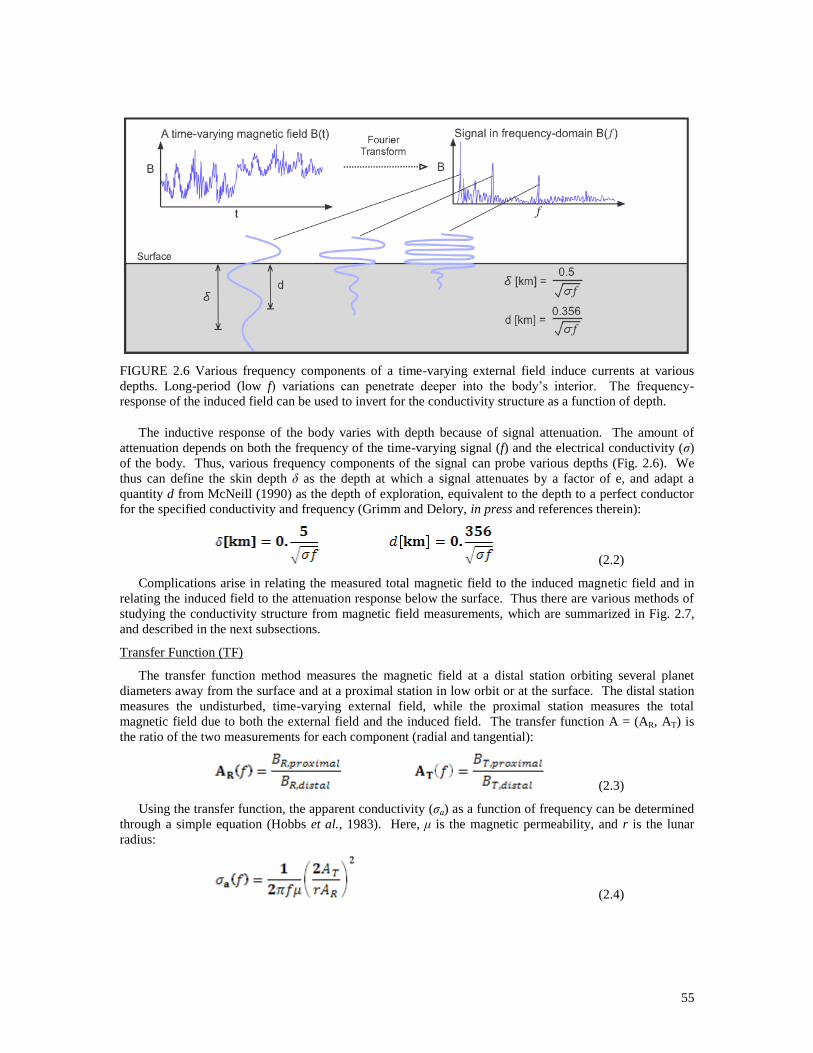
The inductive response of the body varies with depth because of signal attenuation. The amount of
attenuation depends on both the frequency of the time-varying signal (f) and the electrical conductivity (σ)
of the body. Thus, various frequency components of the signal can probe various depths (Fig. 2.6). We
thus can define the skin depth δ as the depth at which a signal attenuates by a factor of e, and adapt a
quantity d from McNeill (1990) as the depth of exploration, equivalent to the depth to a perfect conductor
for the specified conductivity and frequency (Grimm and Delory, in press and references therein):
(2.2)
Complications arise in relating the measured total magnetic field to the induced magnetic field and in
relating the induced field to the attenuation response below the surface. Thus there are various methods of
studying the conductivity structure from magnetic field measurements, which are summarized in Fig. 2.7,
and described in the next subsections.
Transfer Function (TF)
The transfer function method measures the magnetic field at a distal station orbiting several planet
diameters away from the surface and at a proximal station in low orbit or at the surface. The distal station
measures the undisturbed, time-varying external field, while the proximal station measures the total
magnetic field due to both the external field and the induced field. The transfer function A = (AR, AT) is
the ratio of the two measurements for each component (radial and tangential):
(2.3)
Using the transfer function, the apparent conductivity (σa) as a function of frequency can be determined
through a simple equation (Hobbs et al., 1983). Here, μ is the magnetic permeability, and r is the lunar
radius:
(2.4)
FIGURE 2.6 Various frequency components of a time-varying external field induce currents at various
depths. Long-period (low f) variations can penetrate deeper into the body‘s interior. The frequency-
response of the induced field can be used to invert for the conductivity structure as a function of depth.

56
Geomagnetic Depth Sounding (GDS)
Another way to measure apparent conductivity is by taking the horizontal gradient of the tangential
component of the magnetic field. This can be done using two or more magnetometers placed with spacing
comparable to the exploration depth. The ratio between the radial magnetic field and the horizontal
gradient of the tangential magnetic field can be used to determine the apparent conductivity. Here, the
derivative with respect to xT denotes a spatial gradient in the tangential direction (Gough and Ingham,
1983):
(2.5)
Magnetotellurics (MT)
This method measures orthogonal components of the electric (E) and magnetic (B) fields from one
station (Simpsons and Bahr, 2005). Using these measurements, two apparent conductivities can be
calculated using the equations:
(2.6)
The two values will coincide if the medium below is horizontally isotropic in terms of the conductivity.
Thus, comparing the two values can also give an indication of any lateral heterogeneity that might be
present (Grimm and Delory, in press).
FIGURE 2.7 Options for station set-up and requirements for Geomagnetic Depth Sounding (GDS),
Magnetotellurics (MT) and Transfer Function (TF) EM sounding methods. Dashed lines indicate
measurements that need to be performed together. Coordinate systems are also illustrated for each method
(Modified after Grimm and Delory, in press).

57
Lunar Laser Ranging (LLR)
The internal deformation of the Moon can modify its orbit and rotation in subtle ways (Fig. 2.8). A
suite of highly developed mathematical analyses can be used to interpret these movements and give
information about the structure and behavior of the lunar interior. To do so, one must first accurately
measure these subtle lunar wobbles. To date, lunar laser ranging (LLR) is the only viable means of doing
so with the required accuracy (Williams et al., 2006).
For a solid body object in 3-dimensions, its mass distribution is described by a moment of inertia tensor
I. This tensor can be decomposed into three separate tensors, describing the solid mass distribution (Irigid),
the time-varying mass distribution due to tidal deformation (Itide), and the spin-related distortion to the
moment of inertia measurement (Ispin) (Williams et al., 2001):
(2.7)
The rigid-body moment of inertia tensor (Irigid) has eigenvectors associated with the principal axes of
the Moon. The eigenvalues of this coordinate system (A<B<C) are called the rigid-body moments. These
describe the time-averaged mass distribution of a body with respect to each of the principal axes. The
principal axis associated with A is approximately pointing towards the Earth. The axis associated with C is
pointing approximately in the direction of the rotational vector of the moon.
Tidal and rotational affects can act to deform the body with observed monthly variations of ±9 cm
(Williams et al., 2010). These variations depend on the Moon‘s elastic properties, characterized by tidal
Love numbers h2, l2 and k2. These values can be used jointly with seismic data to invert for mantle and
core structure (Merkowitz et al., 2007). Thus, accurate determination of these values will help constrain
the bulk elastic properties of the lunar interior. Love number k2 also depends on any flattening of the core-
mantle boundary (CMB) along the C-axis. The tidal love numbers and the ratios of the principal moments
(A, B and C) can all be determined through accurate measurements of the Moon‘s physical librations. The
existence of a fluid core, size of the outer core, possible inner core and the geometry of the CMB can also
have significant effects on this libration through their interactions with the solid mantle (Williams and
Boggs, 2008).
LLR measures the physical librations by precisely monitoring the positions of various points on the
lunar surface relative to Earth. This can be done by installing retroreflectors on the Moon and measuring
the travel time of the pulses sent to these reflectors that have reflected back to Earth. A retroreflector
network is currently installed on the Moon, but it is limited in both E-W and N-S extent. Increasing this
FIGURE 2.8 Libration and tidal deformation of the Moon. Precession corresponds to circular motion about
the center of mass, whereas nutation corresponds to lateral movement rotating about the center of mass.

58
span would improve the accuracy of the measurements, and would help better constrain the bulk elastic
properties of the lunar mantle, and the size, geometry and state of the core.
Heat Flow Measurements
By measuring the present rate at which a planetary body is dissipating heat, one can learn about not
only the present interior thermal structure but also the thermal history of the body. Knowledge of the
thermal structure of the interior and how it evolved with time can also constrain the density and
compositional stratification of the mantle. In general, thermal energy is dissipated through advection,
conduction and radiation. Advection requires transport of heat-carrying material, which does not happen in
the lunar regolith due to the lack of an advecting medium (e.g. water, air). The regolith material is also
radiatively opaque. Although its porosity allows for radiative transfer within the regolith, it can be treated
as a property of the regolith that affects its thermal conductivity (Kiefer, 2012). Thus, the total heat flow at
the lunar surface can be well approximated by measuring the conductive heat flux. In accordance to
Fourier‘s law of conduction, the conductive heat flux radially outward (qz) is given by:
(2.8)
where z is depth, T is temperature, and k is the thermal conductivity of the material. Therefore, the
measurement of qz requires the determination of both the geothermal gradient and the thermal conductivity.
The geothermal gradient can be measured in boreholes >3 m deep with temperatures taken at different
depths spanning at least 1 m below material affected by the annual and diurnal thermal waves (Kiefer,
2012). The thermal conductivity can be determined through the measurements of the thermal diffusivity
(κ), which is related to the rate at which a material responds to temperature perturbations at various
distances from the perturbation. This can be measured both actively (using a heating source and sensor)
and passively (using periodic changes in surface insolation). The conductivity (k) can then be determined
through the relation, k = κCp, with appropriate values for the specific heat (Cp) and density () assigned.
Gravity Measurements
The sub-surface structure of the Moon can be probed by measuring the gravity field. This can be done
in orbit by tracking the acceleration of a spacecraft as it flies over the surface. The acceleration a
spacecraft experiences depends on the mass distribution:
(2.9)
Here G is the universal gravitational constant, r is the coordinate of the mass element (dm = ρ(r)d r 3), r
is the position of the spacecraft and |r-r | is the distance from the mass element to the spacecraft.
The greatest contributor to changes in acceleration is the mass excess/deficit directly below the
spacecraft. Thus, accurately tracking the changes in position (r) and acceleration of an orbiter as it flies
over a terrain will map the near-surface mass distribution (Stacey and Davis, 2008). To overcome the
difficulty of tracking an orbiter on the lunar farside, a twin satellite approach can be employed. In this
case, one satellite goes over a feature first and accelerates, changing the distance from the satellite behind.
The separation change can be measured and recorded without communication with Earth. This is the
approach taken by the new Gravity Recovery And Interior Laboratory (GRAIL) mission (Zuber, 2008).
The spatial resolution of gravity mapping is comparable to the orbital altitude. Contributions to gravity
anomalies from topographic features (e.g. mounds, craters) can be processed out of the data with
knowledge of the feature‘s average density (i.e., Bouguer correction).
After corrections, the gravity anomaly is a measure of the subsurface density distribution and can give
information about subsurface structure. Any gravity excess/deficit will be due to a combination of
variations in thickness and density of the crust or underlying mantle. One can then use a priori information
concerning density variations to produce global crustal thickness models (Wieczorek et al., 2006). These
models need to be refined/anchored with surface studies (i.e., seismology) of crustal thickness at
representative sites. In addition to crustal information, tracking orbiters can also yield the moment of
inertia (I) of the body, which gives information on internal mass concentration, constraining the existence

59
of a dense core. Temporal variations in the gravity field due to tides can also be measured with an orbiter,
which would constrain tidal Love number k2 (Williams et al., 2010).
GENERAL METHODS
ArcMap 10 geographic information systems (GIS) software and MATLAB were used extensively
throughout the landing site selection process to locate regions which matched the criteria set out for
geophysical and sample return requirements specific to each Science Goal.
Separate project files for geophysical and sample return elements of each Science Goal were produced.
These project files contain all relevant data available to find all the possible landing sites to address that
particular element of the Science Concept. At the end of each Science Goal, geophysical and sample return
maps were combined to find the sites where the most questions may be answered for each Science Goal. In
some cases the geophysical and sample return elements of each Science Goal were not compatible. Finally,
all the maps were brought together to find landing sites that may be appropriate to address Science Concept
2.
There are two global map projections used throughout the report: Plate Carree and Orthographic. Plate
Carree is the most common for global datasets and is centered at 0°E. An orthographic projection is used
when there is a need to emphasize nearside and farside locations and is also centered at 0°E. All
projections use the International Astronomical Union (IAU) 2006 Moon as a reference sphere, which has a
radius of 1,737.4 km (Seidelmann et al., 2007).
DATA
All data used for the landing site selection process are shown in Table 2.2.
TABLE 2.2 All datasets used for Science Concept 2.
Data Resolution Instrument Source Authors
Imagery
WAC Global
Mosaic
64 ppd LRO http://wms.lroc.asu.edu/lroc
/global_product/100_mpp_
global_bw
Digital Terrain Model
LDEM 64 ppd LOLA http://imbrium.mit.edu/DA
TA/LOLA_GDR/CYLIND
RICAL/IMG/
LDEM 128 ppd LOLA http://imbrium.mit.edu/DA
TA/LOLA_GDR/CYLIND
RICAL/IMG/
Crater Records
LPI-CLSE crater
database
N/A N/A http://www.lpi.usra.edu/lun
ar/surface/Lunar_Impact_C
rater_Database_v24May20
11.xls
Losiak et al. (2009);
revised by Ohman
(2011)
LOLA Crater
Database
N/A LOLA http://www.planetary.brow
n.edu/html_pages/LOLAcr
aters.html
Head et al. (2010)

60
Magnetic Data
Internal
magnetic field
1° LP
magnetomet
er and
Clementine
Topography
http://core2.gsfc.nasa.gov/r
esearch/purucker/moon_20
10/index.html
Purucker and Nicholas
(2007)
Element Data
Thorium LP
Titanium LP
Iron LP
Ejecta Material
Crater ejecta
material
Shapefiles Science Concept 5
Other
Sinuous Rilles Shapefiles Hurwitz et al.
(submitted to Planetary
and Space Science,
May 2012)
Floor-Fractured
Craters
Shapefiles Science Concept 5
Pyroclastic
database
Shapefiles Refer to Table A2.2
for references
Cryptomare
deposits
Shapefiles Refer to Table A2.3
for references
Olivine detection Shapefiles Yamamoto et al.
(2010), Table A2.5
Deep
moonquake nest
locations
Nakamura (2005)
Shallow
moonquake
event locations
Nakamura (1977)
Digital Elevation Model (DEM)
The Lunar Orbiter Laser Altimeter (LOLA) 64 and 128 pixels per degree (ppd) gridded datasets were
used to produce a slope map and a map of areas visible from the Earth‘s surface.

61
Imagery
Images used in this study come from the Lunar Reconnaissance Orbiter (LRO) Wide Angle Camera
(WAC) global mosaic. The 64 ppd version of this dataset is used in global maps where higher resolution is
not necessary.
Slope
Slope maps were produced from the LOLA 64 ppd elevation dataset, where the value of the slope
represents the maximum slope between the pixel and one of its neighbors (slope value in degrees). The 64
ppd LOLA DEM was used as it was not deemed necessary to have slope at higher resolution and the only
slope requirement was to land well away from areas of 20°or larger slope.
SCIENCE GOAL 2A: DETERMINE THE THICKNESS OF THE LUNAR CRUST (UPPER AND
LOWER) AND CHARACTERIZE ITS LATERAL VARIABILITY ON REGIONAL AND
GLOBAL SCALES
Introduction
Compared to the relative lack of information regarding the lunar mantle and core, decades of petrologic
and geophysical analyses of the lunar crust have resulted in a significant, but far from complete,
understanding of its thickness, chemistry, and spatial variation across the Moon. For example, it is
generally accepted that (1) the crust is thicker under the primordial highlands than under major impact
basins and mare (Wood, 1973), (2) the farside highlands crust is thicker and more magnesian than the
nearside highlands (Wieczorek et al., 2006; Arai et al., 2008 and references therein), and (3) the crust is
vertically stratified (Toksöz et al., 1974; Ryder and Wood, 1977; Spudis and Davis, 1986; Ryder et al.,
1997; Tompkins and Pieters, 1999) and laterally heterogeneous in thickness (Chenet et al., 2006) and
composition (Arai et al., 2008). Given the work of previous studies, additional geophysical analyses are
key to further understanding the nature and distribution of lunar crustal material. These analyses include
passive seismic experiments and electromagnetic (EM) sounding data, coupled with orbital analyses of the
lunar gravity field (e.g., the ongoing GRAIL mission). These data will provide direct insights about crustal
thickness and better constrain models for lunar crustal formation and evolution.
The purpose of sample return in a crustal thickness context is to better understand the global
geochemistry of the lunar crust, which has important implications for crustal thickness and petrogenesis. It
is widely accepted that the uppermost part of the lunar crust is mainly anorthositic (containing calcic
plagioclase feldspar), whereas the lower crust is more mafic in composition (containing a greater fraction
of olivine and pyroxene) (Ryder and Wood, 1977; Spudis and Davis, 1986; Wieczorek and Zuber, 2001;
Arai et al., 2008 and references therein). However, outcrops of pure anorthosite are limited (Hawke et al.,
2003) and there is evidence of significant lateral and vertical heterogeneity in crustal composition on a
regional (Ryder et al., 1997) to global scale (Arai et al., 2008). Additionally, it has recently been suggested
that compositional variations may correlate to differences in crustal thickness (Cahill et al., 2009). It is
therefore anticipated that sample return will be used to provide compositional context for the geophysical
measurements made. For example, sample return may determine whether a physical or compositional
transition is responsible for a marked change in seismic velocity at ~20 km depth (e.g., Toksöz et al.,
1974).
Science Concept 3 also requires samples of crustal materials and as such many of the requirements and
approaches described here will overlap with that Science Goal. The rocks that will be considered for
sample return are those that can be shown to provide representative compositions of the whole crustal
stratigraphy (upper and lower lunar crust) over regional and global scales.
Background
Thickness of the Lunar Crust
Though suffering from limited data and poor resolution, orbital gravity and laser altimetry studies first
noted the hemispherical dichotomy in crustal thickness, with a farside crust that was proposed to be ~10–15

62
km thicker than that of the nearside (e.g., Wood, 1973; Kaula et al., 1974). Thinner crust was also inferred
under mare basalts (i.e., in large impact basins: Wood, 1973; Kaula et al., 1974). These studies were
complemented by seismic data from Apollo 12, 14, 15, and 16 that placed constraints on crustal thicknesses
at known surface locations (Toksöz et al., 1972, 1974; Goins et al., 1981a). The Apollo 12 and 14 sites
(located <200 km from each other) were interpreted to have crustal thicknesses around 58–65 km (Toksöz
et al., 1972, 1974; Nakamura et al., 1982), compared to the topographically higher Apollo 16 site that
maintained a thicker 75-km crust (Goins et al., 1981a). Both sites showed evidence of a 20-km seismic
discontinuity (Toksöz et al., 1972, 1974; Goins et al., 1981a) that has been interpreted either as a physical
(i.e., due to annealing of impact-related fractures with depth: Simmons et al., 1973) or a compositional
boundary (i.e., a more mafic lower crust overlain by felsic anorthosites: Toksöz et al., 1972, 1974; Ryder
and Wood, 1977; Tompkins and Pieters, 1999). It has also been suggested that a compositionally-stratified
crust may result in a physical fracture discontinuity due to differences in material properties (Wieczorek
and Phillips, 1997).
More recent studies of lunar crustal thickness have tended to either reanalyze the Apollo seismic data
(Khan et al., 2000; Khan and Mosegaard, 2002; Lognonné et al., 2003; Chenet et al., 2006) or utilize
updated gravity and topography datasets (e.g., Clementine: Zuber et al., 1994; Lunar Prospector: Konopliv
et al., 1998, 2001) to calculate global crustal thickness (Zuber et al., 1994; Wieczorek et al., 2006; Hikida
and Wieczorek, 2007; Ishihara et al., 2009; see below). These datasets are not mutually exclusive; seismic
analyses can only determine crustal thickness local to the Apollo Seismic Network (or any future network),
but gravity- and topography-derived datasets require seismic data as pinning points for global models.
Many early gravity-derived models were anchored to ~60 km crustal thicknesses at the Apollo 12 and 14
sites (e.g., Zuber et al., 1994); however, recent seismic reanalyses and gravity models show that the Apollo
12 and 14 sites are likely thinner than proposed by Toksöz et al. (1972, 1974), with various workers
suggesting values of 30–50 km (Khan et al., 2000; Khan and Mosegaard, 2002; Lognonné et al., 2003;
Chenet et al., 2006; Hikida and Wieczorek, 2007; Ishihara et al., 2009). Similarly, the proposed crustal
thickness for the Apollo 16 landing site has also been reduced, for example to 38±7 km (Chenet et al.,
2006) or ~54 km (Hikida and Wieczorek, 2007). Significant discrepancies in proposed crustal thicknesses
exist between gravity- and seismic-derived models (e.g., the gravity model of Ishihara et al. (2009)
compared to the seismic model of Chenet et al. (2006)) and even between models derived from similar
datasets (e.g., the seismic model of Khan et al. (2000) compared to that of Lognonné et al. (2003)),
elucidating the need for further orbiter and surface data collection. (Additional data on crustal thickness are
contained in geoid-to-topography ratio (GTR) and spectral admittance studies; see Wieczorek et al. (2006)
for a compilation.)
Still, a number of important conclusions derived by early studies have been supported. For example,
the farside highlands crust contains the thickest crust (up to ~110 km: Ishihara et al., 2009) and is on
average 10–20 km thicker than the nearside (Zuber et al., 1994; Chenet et al., 2006; Wieczorek et al.,
2006); crustal thickness is at a minimum in large, mare-flooded impact basins such as Crisium, Orientale,
and Moscoviense (Zuber et al., 1994; Wieczorek et al., 2006; Hikida and Wieczorek, 2007); and the 20-km
seismic discontinuity is likely real and may be widespread in the lunar crust (Wieczorek and Phillips, 1997;
Khan et al., 2000; Khan and Mosegaard, 2002). Additionally, there are large lateral variations in the crust,
perhaps relating to heterogeneity in fracture concentrations or the influence of heterogeneous serial
magmatism (Chenet et al., 2006). Finally, the average crustal thickness for the entire Moon is thought to
be around 50 km (Wieczorek et al., 2006; Ishihara et al., 2009), which is useful as a reference value for
future crustal thickness models.
The origin of the hemispherical asymmetry in crustal thickness is less clear. Early studies correlated
this anomaly to the nearside concentration of mare basalts and KREEP, and the center-of-mass/center-of-
figure offset (e.g., Wood, 1973; Kaula et al., 1974) and suggested their coupled derivation from asymmetric
asteroid bombardment (Wood, 1973) or asymmetric crustal growth (Warren and Wasson, 1980; Arai et al.,
2008). Recent work has considered the influence of either internal asymmetries in LMO convection (Loper
and Werner, 2002) and tidal dissipation (Garrick-Bethell et al., 2010) or external asymmetries such as the
distribution of SPA ejecta (Zuber et al., 1994; Arai et al., 2008). Accretion of a companion moon to the
lunar farside has also been proposed (Jutzi and Asphaug, 2011). Further discussion is beyond the scope of
this work, but increased understanding of crustal thickness and its variability will help constrain the
accuracy of these models and contribute to knowledge of early lunar formation.
63
Recent and Ongoing Gravity Datasets (esp. for Crustal Thickness)
The most widely used lunar gravity map to model crustal thickness was developed using data from
Lunar Prospector, which was launched by NASA in 1999. These data were taken by measuring Doppler
shifts in the microwave-tracking signal as it reaches Earth, and converted into acceleration to provide
information on the gravity field (Konopliv et al., 1998). This method has only been able to indirectly map
the farside of the Moon due to the lack of line-of-site communication with Earth, and as such the precision
and reliability of farside gravity maps is uncertain. SELENE Kaguya first directly mapped the farside
gravity field on the Moon by using four-way Doppler tracking with relay sub-satellite Okina, launched by
JAXA in 2007 (Namiki et al., 2009), which has already significantly improved the accuracy of farside
gravity maps (e.g., Ishihara et al., 2009).
The ongoing Gravity Recovery and Interior Laboratory (GRAIL) mission, launched by NASA in 2011,
consists of two near-identical lunar orbiters, a leader (Ebb) and a follower (Flow), that measure a
microwave beam transmitted between them to find their relative position (assisted by GPS) from which
variations in the Moon‘s gravity can be extracted. The first stage has successfully mapped global gravity
variations from a 50 km altitude with a spherical harmonic degree of 330, improving current lunar gravity
data maps from SELENE by 3× on the nearside (previous spherical harmonic degree of 110) (Konopliv et
al., 2001) and 5× on the farside (previous spherical harmonic degree of 70) (Matsumoto et al., 2010).
During the second stage, GRAIL will perform high-resolution (30 km × 30 km) mapping to a higher
accuracy of <1 mGal (1 mGal = 0.01 m/s2) (W. Kiefer, pers. comm.) with a tracking error of <0.1 μm/s
(Weaver et al., 2010).
The main objectives of GRAIL are to determine the structure of the lunar interior from crust to core
(Science Goal 2a and 2c) and to advance understanding of the thermal evolution of the moon (Science Goal
2d). In particular, GRAIL investigations will include:
Mapping crustal and lithospheric structure (combined with LOLA topography data)
Ascertaining temporal evolution of crustal brecciation and magnetism
Determining subsurface structure of impact basins and mascon (―mass concentration‖) origin
Understanding asymmetric lunar thermal evolution
Constraining deep interior structure from tides
Placing limits on size of a possible solid inner core
Since these objectives directly correlate to Science Concept 2 (in particular Science Goals 2a, 2c, and
2d), the completion of the GRAIL mission and subsequent release of data will greatly contribute to the
work that is outlined here.
Deriving Crustal Thickness from Gravity
The gravity anomaly map is used in conjunction with a high-resolution topographic map to model the
Moon‘s crustal thickness, primarily by subtracting the gravitational effects from surface topography (e.g., a
crater or mountain), amongst other corrections. This method is illustrated as a flow diagram in Fig. 2.9.
These models can be further constrained and improved by using passive seismic nodes with known crustal
thicknesses as anchor points (e.g., Chenet et al., 2006).
For the purposes of this report, we use crustal thickness models derived from Lunar Prospector data and
Clementine topography (Wieczorek et al., 2006), as complete Kaguya SELENE and GRAIL data are not
yet publicly available. However, we note that preliminary results are available in the literature; the most
recent iteration of lunar crustal thickness models uses combined SELENE gravity and topography data
(Ishihara et al., 2009), and these models will be superseded by GRAIL‘s high-resolution gravity data
combined with the LRO LOLA topography map.
Composition and Petrogenesis of the Lunar Crust
A full understanding of crustal thickness requires consideration of crustal composition, particularly to
provide constraints to seismic and gravity/topography models (e.g., density) of the lunar crust.
Additionally, compositional constraints are required to formulate models for the crustal formation and
evolution that can explain crustal thickness distributions.

64
Considering the constraints from LMO differentiation models, the Al-rich anorthositic upper crust is
thought to have formed directly from the magma ocean by plagioclase flotation (Wood et al., 1970), though
others have suggested the influence of more complicated processes involving reprocessing of primitive
crust (e.g., Walker, 1983; Longhi, 2003; Meyer et al., 2010). In contrast, petrologic and remote sensing
studies indicate that the lower crust is more mafic but still contains plagioclase (Ryder and Wood, 1977;
Pieters et al., 1997; Ryder et al., 1997; Wieczorek and Zuber, 2001; Arai et al., 2008 and references
therein). A possible explanation for this difference is that the latest LMO liquids became denser and more
Fe-rich after the removal of Mg-rich olivine and pyroxene, which allowed certain mafic minerals to float
along with plagioclase (Wieczorek and Zuber, 2001). Alternative theories suggest underplating by mare
basalt liquids (Head and Wilson, 1992) or that the lower crust is composed of various mafic intrusive rocks
(Ryder and Wood, 1977) which could represent a phase of post-magma ocean serial magmatism (e.g.
Warren, 1993; Ryder et al., 1997; Longhi, 2003). One item that remains unclear is the crust-mantle
distribution of primitive urKREEP.
FIGURE 2.9 Flow diagram indicating the steps taken to produce a global crustal thickness model for the
Moon. Global gravity datasets (e.g., from Clementine, Lunar Prospector, Kaguya SELENE, and GRAIL)
are combined with topographic datasets (e.g., from Clementine, Kaguya SELENE, and LOLA), corrected,
and inverted for crustal thickness (e.g., Model 3 from Wieczorek et al., 2006, shown here).
Although the LMO is a convenient and accepted framework for lunar crust formation, geophysical and
petrologic studies have shown that the lunar crust is not simply stratified but highly variable both laterally
and vertically. Based on remote sensing data from the Clementine mission, Jolliff et al. (2000) defined
four geochemical terranes with distinct major and trace element abundances: the Procellarum KREEP
Terrane (PKT), Feldspathic Highlands Terrane (FHT) (further subdivided into FHT-A, for ―anorthositic,‖
and FHT-O, for ―other‖) and the South Pole Aitken Terrane (SPA or SPAT). Lateral crustal heterogeneity
is also indicated by hemispherical asymmetry in crustal composition: whereas ferroan anorthosites are

65
thought to overlie a noritic lower crust (orthopyroxene + plagioclase) on the lunar nearside, the farside crust
is proposed to consist of magnesian anorthosites overlying Mg-rich troctolites (olivine + plagioclase)
(Takeda et al., 2006; Arai et al., 2008, Ohtake et al., 2009, 2012). Furthermore, the nearly exclusive
nearside distribution of basaltic maria, while not directly bearing on crustal composition, may stem from
the same process that resulted in lateral heterogeneity.
Vertical variability in crustal composition further complicates the simple LMO differentiation story.
Global remote sensing data shows that the highlands crust is not composed of extensive areas of anorthosite
(e.g., Lucey et al., 1995), but that the largest areas of anorthosite are exposed in impact craters and basins,
especially in rings formed during crater modification stages (Hawke et al., 2003). This suggests that the
original upper crust has been significantly reworked and modified by impacts and volcanism on various
scales, and that the principal layer of anorthosite underlies impact-excavated megaregolith (Taylor, 2009)
with a possible mafic ―mixed layer‖ that represents a primordial, quenched LMO crust (Hawke et al.,
2003). In addition, the ejecta of large impact basins are more mafic than the surrounding highlands, as are
the central peaks and peak rings of select complex craters (Pieters et al., 1997). Similarly, the SPA basin
floor is notably more mafic in composition than the surrounding FHT (Pieters et al., 1997). These lateral
and vertical complexities in crustal composition require further review and refinement of the simple LMO
model for crustal formation.
Petrology of the lunar crust – inferences from sample studies
Previous studies of Apollo and Luna samples have organized pristine non-mare rocks into 3 broad
groups: the ferroan anorthosite suite (FAS), the magnesian suite (Mg-suite), and the alkali suite (e.g.
Warren, 1993; Taylor, 2009). As defined by Warren and Wasson (1978), ‗pristinity‘ is a term used to
distinguish those rocks that have survived significant modification (physically and chemically) by impacts.
Fig. 2.10 illustrates the compositional and geochemical variations among the highlands lithologies, as well
as the approximate locations of these within the crust.
Ferroan Anorthosite Suite (FAS)
Generally, the FAS rocks are composed of ~77 to 96 vol. % Ca-rich (anorthite) plagioclase feldspar
(Fig. 2.12) having relatively high Al2O3 compositions (Wieczorek et al., 2006). The mafic silicate minerals
in the FAS have low Mg# (molar Mg/(Mg+Fe)), indicating the ferroan nature of the FAS (Taylor et al.,
1991; Wieczorek et al., 2006). The FAS also display low concentrations of incompatible elements (e.g., Th
and La) and have large positive europium (Eu) anomalies (Taylor et al., 1991). The FAS can be further
subdivided on the basis of modal mineralogy and composition (e.g., Taylor, 2009). For example, the pure
anorthosite (PAN) has a plagioclase content of >95 vol. %, FeO <3 wt. % and an An 70-90 plagioclase
composition (e.g. Ohtake et al., 2009). The range in compositions and ages displayed by the FAS suggests
that they likely represent the primary crystallization products of the LMO (e.g. Norman and Ryder, 1979;
Taylor, 2009).

66
FIGURE 2.10 From left to right, the image illustrates the rock name, the corresponding plagioclase-olivine-
pyroxene ternary composition diagram (where 90, 77.5, 60, 10 indicate the relevant % plagioclase), two
rare earth element spider diagrams highlighting the difference in composition between the FAN and
proposed super-KREEP (after Taylor, 2009) with respective positive and negative Eu anomalies, and
finally where the rocks may be found within lunar crust-mantle stratigraphy. Color scheme is consistent
throughout this chapter. Modified from Jolliff (2012).
Mg-suite
The Mg-suite lithologies contain less feldspar than the FAS (<80 vol. %, Fig. 2.12) (Taylor, 2009). The
lithologies constituting the Mg-suite are norite, troctolite, and dunite. The Mg-suite is geochemically
unusual in that it is relatively enriched in trace elements (i.e., KREEP) indicating a highly evolved parental
magma, but its Mg# (>64) suggest a primitive parental magma (Wieczorek et al., 2006). Petrologic studies
of the Mg-suite samples suggest that they represent intrusions into the primary lunar crust and are possibly
the result of serial magmatism post-LMO crystallization (Taylor, 2009 and references therein). Two
petrogenic models have been developed for the Mg-suite: Model 1 involves decompression melting and
rising of highly magnesian early LMO cumulates, which assimilated with the late LMO urKREEP; Model
2 suggests that hybridized mantle cumulates and urKREEP were the source for Mg-magmas as a result of
massive overturn (Shearer and Papike, 2005).
Alkali suite
The alkali suite includes KREEP basalt, alkali anorthosite, alkali gabbronorite, quartz monzodiorite, and
felsite, all of which are rocks enriched in alkali elements (Taylor, 2009). The alkali suite contain ~50 vol.
% plagioclase, with bulk Al2O3 ranging from 13 to 16 wt. % and Mg# between 52 and 65 (reviewed by
Wieczorek et al., 2006). This suite displays a typical KREEP incompatible element enriched signature
(Taylor, 2009) (Fig. 2.12). Although most lunar basalt samples have a KREEP component, actual KREEP
basalts are only found in the Apollo 15 sample collection (Wieczorek et al., 2006). Petrological models
evoke the possibility that the fractional crystallization of KREEP basalt created the cumulate diversity seen
in the alkali suite samples, and that the parentage of KREEP basalt is more applicable to the alkali suite
than the Mg-suite (e.g., as shown by experimental studies of quartz monzodiorite) (e.g. Taylor, 2009). The
alkali suite crystallization ages range from ~4.3 to 3.8 Ga, overlapping that of the FAS and Mg-suite
(Wieczorek et al., 2006).
A significant problem with these studies to date is that the sample collection is limited to rocks from the
PKT, and it is unclear how well these lithologic groupings apply to the entirety of the lunar crust (e.g.,
Cahill et al., 2009). In order to better understand asymmetry in crustal thickness, determine its relationship

67
to chemical stratification, and gain better understanding of urKREEP chemistry and its distribution at the
crust-mantle boundary, samples from all geochemical terranes and the full stratigraphy of the crust need to
be collected. These data can also constrain the chemical and physical properties of the medium in
geophysical models.
Using Impact craters as windows into the lunar interior
Impacts drill holes deep into the lunar subsurface, excavating and exposing this material in crater
deposits and landforms. We have utilized equations, which are briefly described below, to calculate which
craters or basins on the lunar surface may expose upper and lower crust material. For a more detailed
discussion please refer to the Methodology section in Science Concept 3.
For simple craters (craters with diameter less than approximately 16–20 km), the transient crater
diameter (Dtc) can be calculated using Equation (2.10), where D represents the final diameter of the crater
(all in km):
Dtc = 0.84D (2.10)
For complex craters, we utilized Equation (2.11) to determine the transient crater diameter (after Croft,
1985), where Dsc is the transition crater diameter from simple to complex craters (approximately 16–20 km
on the case of the Moon) and all parameters are in cm:
D = Dsc-0.18
Dtc1.18
(2.11)
The Dtc was then used in the following equations to calculate the maximum depth of excavation (de) and
maximum depth of melting (dm). These two key parameters were compared against three models of crustal
thickness from Wieczorek et al. (2006) (as discussed in the Science Concept 3 methodology section).
Depth of excavation
Ejecta deposits are material mobilized from the site of impact onto the surrounding terrane. The ejecta
material does not come from the full depth of the crater but rather from much shallower levels (Melosh,
1989). The maximum depth from which the ejecta material originates is determined by calculating the
depth of excavation (de) (Equation 2.12: Croft, 1980; Melosh, 1989), which is important for determining
the contribution of crust/mantle components. de is generally equal to one third of the transient crater depth
dtd, or one tenth of the transient crater diameter Dtc (all in km):
De = 1/3Dtd = 1/10Dtc (2.12)
Maximum depth of melting
The maximum depth of melting (dm) for complex craters, i.e., those with diameters >16–20 km, is
calculated by Equation (2.13) (after Cahill et al., 2009), where D is the final rim diameter of the crater in
kilometers:
Dm = 0.109D1.08
(2.13)
For all complex craters with a diameter >20 km listed in the Lunar Impact Crater Database (Losiak et
al., 2009, revised by Ohman, 2011), the proximity to the crust-mantle boundary was calculated by
subtracting either the depth of excavation or depth of melting, from the pre-impact crustal thickness (as
determined by each of the three crustal thickness models) (after Cahill et al., 2009). Where a positive
proximity means that de or dm is located only within the crust and a negative proximity means that de or dm
may extend into the mantle.
Impact melt sheet
An impact melt sheet is formed due to the vast amount of kinetic energy generated during an impact,
which melts the target lithology and any residual impactor material (e.g. Kring, 1995). In the case of
complex (or larger) craters most of the melt pools inside the transient cavity of the crater and creates the
central melt sheet, while some is deposited on crater walls or in terraces and a smaller proportion is mixed
with broken up material and ejected from the crater. The maximum depth of melting allows consideration
of a maximum depth of origin for the melt material.

68
Central peak
Central peaks are formed in complex craters. They result from the shock-compression of material
directly beneath where the impactor hit, which rebounds or recoils back towards the surface, finally resting
above the apparent crater floor (Fig. 2.11; Baldwin, 1974). As concluded by Cintala and Grieve (1998), the
minimum depth of origin for a central peak coincides with the maximum Dm (Equation 2.13). Thus the
maximum dm can be used to determine where within the crust or mantle the central peak material has come
from.
FIGURE 2.11 Schematic cross section of a complex crater with crater deposits and landforms identified.
Notice that the central peak can contain outcrops of uplifted material from deeper stratigraphic levels than
sampled elsewhere in the crater. Not to scale.
Central peak ring or basin inner ring
There are several hypotheses for the formation of peak rings within peak ring craters and multi-ring
basins (Fig. 2.12). Unlike the case for central peaks where the maximum depth of melting likely
corresponds to the minimum depth of origin for the peak material, after Cintala and Grieve (1998) the peak
ring formation is considered to be intrinsically affected by impact melting. They conclude that the material
for the peak ring likely does not come from the maximum depth of melting but from much shallower levels,
and that this applies to peak ring basins and multi-ring basins.
However some workers have also proposed that the central peak ring is an enlargement of a central
peak (e.g. Kring, 2005), thought to be formed from the collapse and spreading of a central peak if it has
risen too far above the surface. Please note that the formation of rings in multi-ring basins is poorly
understood and the reader is redirected to Pike and Spudis (1987) for a comprehensive discussion.

69
FIGURE 2.12 Schematic cross section of a peak ring basin (which is also applicable to a multi-ring basin).
The figure illustrates that breccia and ejecta material can potentially contain material from all levels
sampled by the crater. Note the homogenization of the crustal material from multiple stratigraphic levels in
the massive melt sheet. Not to scale.
Requirements
Orbital Geophysics
Gravity Surveying
Surveying the gravitational field is the best way to characterize both regional and global crustal
thickness variations. This will be completed to a high degree of spatial resolution (~27 km globally) by the
current GRAIL mission (Zuber et al., 2012; Hirt and Featherstone, 2012). Since this data can be obtained
from orbit, it is not considered when selecting landing site locations.
In situ Geophysics
Seismology
While gravity surveys provide a direct measure of the subsurface mass concentration variation, the
crustal thickness (H) itself is modeled from these surveys and requires anchor points where H is known to a
higher degree of certainty. A passive seismic experiment can be used to invert for H both at the
seismometer location and at surrounding locations where meteoroid impacts occur (Chenet et al., 2006). To
maximize the usefulness of these anchor nodes, they need to be positioned at locations representative of the
‗typical‘ crustal thickness for each terrane (Jolliff et al., 2000). Thus, a minimum of four seismometers is
required (one in each terrane), and passive seismic experiments must be implemented concurrently to
obtain maximum constraints for subsequent analyses. Active seismic experiments are not appropriate for
this Science Goal as they do not provide information below ~500 meters depth (Watkins and Kovach,
1972).
EM Sounding
EM sounding can be used in conjunction with seismology to further constrain crustal thickness at the
anchor points. Magnetotellurics (MT) is perhaps the most suitable method, as it does not require an orbital
station (c.f., Geophysical Methods). Detection of the shallow crust requires an EM field signal above 10
Hz, though well-documented fields on the Moon are ≤ 10 Hz in frequency (Grimm and Delory, 2010).
Fortunately, solar wind fluctuations produce robust signals up to 100 Hz, allowing for detection of the
crust-mantle boundary (Fillingim et al., 2010). For Science Goal 2a, MT measurements must be conducted
at the same location as the seismic experiments, but has no requirements of its own as to where the
experiment should be done.

70
Sample Return
Landing sites should be selected to obtain samples that are representative of both the upper and lower
crustal compositions laterally and vertically, specifically:
1. Rocks of both the upper (anorthosite) and lower (norite, troctolite, or gabbro) crust representing
the full compositional range of crustal stratigraphy.
2. Rock samples from each of the four geochemical terranes (after Jolliff et al., 2000).
In order to maximize the probability of successful sampling, selected landing sites should also meet the
following criteria:
3. Outcrops and deposits of a specific basin should be known so that it is clear which crater or
basin is being sampled.
4. Outcrops or deposits should be exposed at the surface and easily accessible.
Methodology
In situ Geophysics
The terranes (as identified by Jolliff et al., 2000) were first traced out in ArcMap 10. To find regions of
‗typical‘ crustal thickness, crustal thickness distributions were extracted and plotted in MATLAB to find
the mean and the standard deviation of crustal thickness for each terrane individually (Fig. 2.13). The
Model 3 total crustal thickness model data from Wieczorek et al. (2006) was used, which is derived from
Clementine topography, and Lunar Prospector LP150Q gravity model data. This model will be replaced
with a model which makes use of LOLA topography and GRAIL data, when the latter becomes available.
ArcMap 10 was then used to extract locations where crustal thickness is within one standard deviation (σ)
of the mean crustal thickness for each terrane, to map areas of ‗typical‘ crustal thickness.
As EM sounding can be carried out anywhere on the lunar surface, there is no mapping required for this
method. This means that Fig. 2.14 is the only map for the geophysical methods within this Science Goal.
Sample Return
In the context of the NRC report, landing site candidates require exposures of rocks that have originated
from deep within the Moon. To fulfill the requirements outlined above, only those craters and basins that
potentially sample the full stratigraphy of the lunar crust have been considered. We have used the
following approach, discussed in more detail in Science Concept 3 (e.g., Flahaut et al., 2012).
1. We utilized the Lunar Impact Crater Database (Losiak et al. 2009, revised by Ohman, 2011) to
identify all craters and basins that may expose the lower crust in either ejecta blankets, melt
sheets, or central uplifts (i.e., central peaks and peak rings). We sought to identify those craters
and basins that tapped both the lower and upper crust, assuming that a crater sampling the lower
crust must have sampled the upper crust as well.
2. Using Equations 2.10–2.13 (outlined above), we identified all craters or basins that may
theoretically expose lower crustal material in their ejecta.
3. Melt depth proximity calculations were used in combination with (1) to determine where the
lower crust may be sampled in impact melt sheets or in central peaks and peak rings (if
preserved).
4. The calculations described above are theoretical and as such LROC Quickmap was used to
verify whether craters/basins did indeed preserve their central peaks or peak rings.

71
FIGURE 2.13 A histogram showing the frequency distribution of ‗thin‘, ‗typical‘, and ‗thick‘ crustal
thickness for each of the terranes, as defined in Jolliff et al. (2000). ‗Typical‘ crustal thickness is defined
as ±1σ of the mean crustal thickness of the terrane (middle vertical line). Lighter shades denote ‗thin‘ crust
for each terrane; darker shades denote ‗thick‘ crust for each terrane. Color scheme is also used in Fig. 2.16
However, there are a number of sampling details that must be considered:
1. The calculations for dm have been used here to determine where the material for the peak rings
comes from. However, there is significant debate regarding how the rings are formed, which in
turn dictates what depth the material comes from. Therefore the rings which have been
identified here as potentially sampling the lower crust should be treated with caution.
2. Only lower and upper crustal exposures within basins are considered. As an example, Imbrium
has a basin diameter of ~1160 km and is theoretically likely to contain lower crust and mantle
material in its ejecta deposits, melt sheet or uplifted central peak or peak rings. However,
Imbrium does not have a well preserved central peak or peak ring, as most of the melt sheet has
been covered with mare basalts and megaregolith. Thus it is likely that samples of mantle
material may be preserved within the basin itself, but most are likely not available for easy
sampling and would be difficult to identify. On the other hand, ejected mantle material may be
well preserved given the relative age of the basin, but the temporal connection between ejected
samples and specific impacts is difficult to verify.
3. As of yet there are no contour maps for ejecta material on the Moon, and modeling has
suggested that deeper material is more likely to be exposed closer to the central uplifts of
craters and basins. Therefore our focus is on sampling the rim ejecta material, as material
further away from the crater is more likely to be buried by regolith (which is particularly true
for older craters).
4. Similarly, larger craters and basins are filled with younger volcanic deposits that obscure the
underlying melt sheet. Thus the most optimal place to sample the melt sheet is where it is
preserved in crater walls or terraces.

72
5. In cases where the central peak or peak ring are preserved, there are likely to be steeply inclined
outcrops of rock that are good places to sample either directly or in debris at the base of the
uplift.
Suggested Landing Sites
In situ Geophysics
Locations where crust is ‗thick‘ (>1σ from the mean), and ‗thin‘ (< 1σ from the mean) are shown in Fig.
2.14 as darker and lighter shades respectively. In accordance to the geophysical requirements, one seismic
station needs to be placed within each of the terranes, and at a location with ‗typical‘ crustal thickness,
which is defined as within 1σ of the mean modeled crustal thickness.
Sample Return
Locations that satisfy the above requirements are shown in Fig. 2.15. All results are displayed in Table
A2.1. Based on proximity calculations, the following craters (identified in Fig. 2.15) have ejecta
potentially containing lower crust material: Nectaris, Orientale, South Pole-Aitken, Ingenii, Poincare,
Antoniadi, and Minkowski (the latter four are located within SPA). Figure 2.17 shows craters and basins
that may have lower crustal material in their melt and preserved central peaks (e.g., Humboldt, Zeeman).
Figure 2.17 also shows craters and basins that may have lower crust material in their melt and preserved
peak rings (e.g., Schrödinger, Orientale, Moscoviense). As noted above, our recommendation is to sample
at least one crater or basin within each terrane; however, note that no craters were identified within the PKT
according to our method. We do not feel that this is a drawback, as Apollo breccias from the PKT may
contain clasts of crustal lithologies.
It should be noted that only specific areas within craters and basins can be sampled to attain upper and
lower crustal compositions. Examples of complex crater (Humboldt) and multi-ring basin (Orientale)
sample locales are illustrated below. However it is important to recall that the formation of peak rings is
poorly understood and that the application of proximity calculations to determine the depth of origin of
peak ring material is somewhat ambiguous.

73
FIG
UR
E 2
.14
Map
sh
ow
ing
th
e ar
eas
of
‗th
in‘,
‗ty
pic
al‘,
an
d ‗
thic
k‘
cru
stal
th
ick
nes
s fo
r ea
ch o
f th
e te
rran
es,
as d
efin
ed i
n J
oll
iff
et a
l.
(20
00
), t
o i
den
tify
sit
es w
her
e it
wo
uld
be
pre
fera
ble
to
pla
ce s
eism
om
eter
s to
aid
ou
r u
nd
erst
and
ing
of
Sci
ence
Go
al 2
a.
Lig
hte
r sh
ades
den
ote
‗th
in‘
cru
st f
or
each
ter
ran
e; d
ark
er s
had
es d
eno
te ‗
thic
k‘
cru
st f
or
each
ter
ran
e.
Th
is m
ap i
s al
so u
sed
fo
r h
eat
flo
w m
easu
rem
ents
,
un
der
Sci
ence
Go
al 2
c an
d 2
d,
as t
his
ex
per
imen
t al
so r
equ
ires
‗ty
pic
al‘
cru
stal
th
ick
nes
s, b
ut
wit
h a
dd
itio
nal
req
uir
emen
ts.
Th
e co
lors
of
def
ined
reg
ion
s co
rres
po
nd
wit
h t
he
co
lors
of
the
his
tog
ram
in
Fig
. 2
.15
.
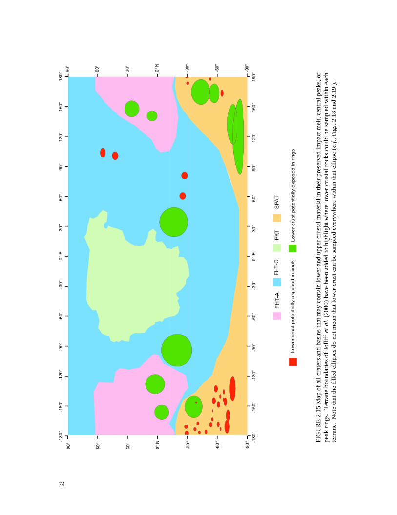
74
FIG
UR
E 2
.15
Map
of
all
crat
ers
and
bas
ins
that
may
co
nta
in l
ow
er a
nd
upp
er c
rust
al m
ater
ial
in t
hei
r p
rese
rved
im
pac
t m
elt,
cen
tral
pea
ks,
or
pea
k r
ing
s.
Ter
ran
e bo
und
arie
s o
f Jo
llif
f et
al.
(2
00
0)
hav
e b
een
ad
ded
to
hig
hli
gh
t w
her
e lo
wer
cru
stal
ro
cks
cou
ld b
e sa
mp
led
wit
hin
eac
h
terr
ane.
N
ote
th
at t
he
fill
ed e
llip
ses
do
no
t m
ean t
hat
lo
wer
cru
st c
an b
e sa
mp
led e
ver
yw
her
e w
ith
in t
hat
ell
ipse
(c.
f.,
Fig
s. 2
.18
an
d 2
.19
).

75
Example 1: Humboldt
Humboldt is presented here as an example of where different lithologies are present within a complex
crater. Humboldt has a preserved central peak (Fig. 2.16) and within this crater it should be possible to
sample ejecta on the crater rim, melt (as this crater has not been flooded with mare basalt), and the outcrops
of the central peak. An example landing site (pink star) been added for perspective; this site could
potentially contain exposures of the lower crust and melt sheet.
Example 2: Orientale
Orientale basin has been selected as an example of where to sample the crust within a multi-ring basin
(Fig. 2.17). Due to the formation mechanisms of multi-ring basins, it is unlikely that all of the rings contain
material from the maximum depth of melting; the inner rings are the most plausible candidates. Figure
2.17 illustrates that though most of the Orientale basin has been flooded with mare basalts that have
covered most of the melt sheet, there may be melt preserved as ponds on basin walls. The inner rook ring
of Orientale is very likely to contain exposures of the LMO-generated crust beneath a megaregolith (e.g.,
Hawke et al., 2003).

76
FIG
UR
E 2
.16
L
RO
C W
AC
Q
uic
km
ap im
age
of
Hu
mbo
ldt
crat
er l
oca
ted
at
26
.8˚
S,
80
.8˚
E.
Th
e to
po
gra
ph
ic p
rofi
le w
as
ob
tain
ed
fro
m
Qu
ick
map
to
ols
u
sin
g
GL
D10
0;
ver
tica
l
exag
ger
atio
n is
~
20
:1.
T
he
cen
tral
p
eak
o
utc
rop
an
d m
elt
po
cket
s co
uld
b
e sa
mp
led
to
o
bta
in
sam
ple
s o
f th
e lo
wer
cru
stal
co
mp
osi
tio
n a
nd
sh
ou
ld b
e sa
mp
led
.
FIG
UR
E
2.1
7
LR
OC
W
AC
Q
uic
km
ap
imag
e o
f O
rien
tale
bas
in l
oca
ted
at
19
.6˚
S,
94
.0˚E
. T
he
top
ogra
ph
ic p
rofi
le w
as
ob
tain
ed
fro
m
Qu
ick
map
to
ols
w
hic
h
use
d
GL
D10
0
dat
a
sou
rce;
v
erti
cal
exag
ger
atio
n
is
~
10
:1.
P
eak
ri
ng
s m
ay
po
ten
tial
ly
con
tain
o
utc
rop
s o
f m
ater
ial
up
lift
ed
fro
m
the
low
er c
rust
.
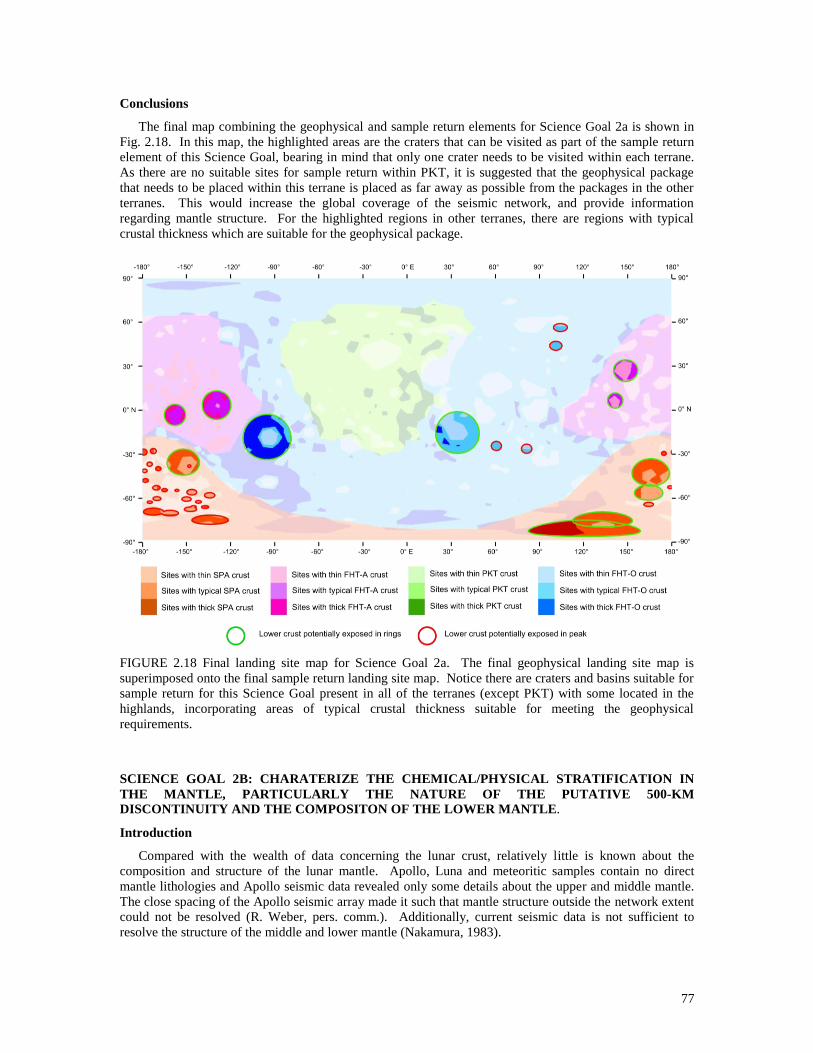
77
Conclusions
The final map combining the geophysical and sample return elements for Science Goal 2a is shown in
Fig. 2.18. In this map, the highlighted areas are the craters that can be visited as part of the sample return
element of this Science Goal, bearing in mind that only one crater needs to be visited within each terrane.
As there are no suitable sites for sample return within PKT, it is suggested that the geophysical package
that needs to be placed within this terrane is placed as far away as possible from the packages in the other
terranes. This would increase the global coverage of the seismic network, and provide information
regarding mantle structure. For the highlighted regions in other terranes, there are regions with typical
crustal thickness which are suitable for the geophysical package.
FIGURE 2.18 Final landing site map for Science Goal 2a. The final geophysical landing site map is
superimposed onto the final sample return landing site map. Notice there are craters and basins suitable for
sample return for this Science Goal present in all of the terranes (except PKT) with some located in the
highlands, incorporating areas of typical crustal thickness suitable for meeting the geophysical
requirements.
SCIENCE GOAL 2B: CHARATERIZE THE CHEMICAL/PHYSICAL STRATIFICATION IN
THE MANTLE, PARTICULARLY THE NATURE OF THE PUTATIVE 500-KM
DISCONTINUITY AND THE COMPOSITON OF THE LOWER MANTLE.
Introduction
Compared with the wealth of data concerning the lunar crust, relatively little is known about the
composition and structure of the lunar mantle. Apollo, Luna and meteoritic samples contain no direct
mantle lithologies and Apollo seismic data revealed only some details about the upper and middle mantle.
The close spacing of the Apollo seismic array made it such that mantle structure outside the network extent
could not be resolved (R. Weber, pers. comm.). Additionally, current seismic data is not sufficient to
resolve the structure of the middle and lower mantle (Nakamura, 1983).

78
The nature of the lunar mantle is highly dependent on details regarding the lunar magma ocean (LMO)
hypothesis, many of which are debated and/or unknown. Mantle composition is governed by the bulk
composition of the Moon and the extent to which the LMO differentiated. Mantle stratification is likewise
dependent on the depth of the LMO, in addition to the degree of stratification during differentiation and the
extent and scale of cumulate overturn. The distribution of deep moonquakes (DMQ) and high frequency
teleseismic events (HFT) indicate at least some mantle stratification with low-velocity zones and structural
discontinuities proposed at various mantle levels, including a major 500-km discontinuity. However, many
of the models that arrived at these features are non-unique, suffer from a dearth of data, or are speculative,
and even those that are more highly resolved lack key constraints.
Science Concept 3 (Science Goal 3a, b, c), Science Concept 5, and Science Concept 6 (Science Goal
6c) have proposed to sample lithologies that will address the composition of the mantle. Sample locations
presented here should be used in conjunction with those other proposed landing sites in order to more
readily address Science Goal 2b. No other Science Concepts have proposed geophysical landing sites that
will address the structure of the mantle.
Background
Lunar Magma Ocean (LMO) and Cumulate Overturn
The lunar magma ocean and subsequent cumulate overturn are discussed in depth in the general
background, and only summarized here. While the nature of the lunar mantle is subject to significant
debate, it is generally agreed that the initial physical and chemical stratification was produced by
differentiation from a magma ocean (e.g., Shearer and Papike, 1999). Prior to any overturn, the LMO
cumulate pile would have been zoned from Mg- and olivine-rich at its base to Fe-, Ti-, KREEP-, and
pyroxene-rich at the top, with a feldspathic crust. Subsequent overturn driven by gravitational instabilities
(Hess and Parmentier, 1995) may have resulted in the delivery of dense ilmenite- and KREEP-bearing
plumes to the middle and lower mantle, creating a ―hybrid‖ heterogeneous mantle source for mare basalts
and pyroclastic glasses, and perhaps resulting in an ensuing series of positively buoyant plumes (e.g,
Singletary and Grove, 2008). These data all indicate that the global zoned structure of the early mantle has
been highly disrupted after its initial solidification, but the extent and scale of mantle heterogeneity is as yet
unclear.
High-Frequency Teleseismic (HFT) Events and Upper Mantle Structure
Twenty-eight out of the ~12,500 seismic events recorded by the Apollo Passive Seismic Experiment
(APSE) were classified as ―high-frequency teleseismic events,‖ characterized by their high-frequency
nature, well-defined P- and S-wave arrivals, and higher-magnitude energy release (Nakamura et al., 1974,
1979; Nakamura, 1977; Oberst, 1987). Unlike deep moonquakes, their occurrence is not aligned with tidal
periodicities (Nakamura et al., 1974; Nakamura, 1977), but is rather statistically correlated with the sidereal
month, such that HFT events tend to occur during a specific lunar orientation relative to the stars (Frohlich
and Nakamura, 2006).
The source depths for HFT are poorly resolved. Though some studies locate epicenters in the shallow
mantle at ~50–200 km depth (Nakamura et al., 1979; Khan et al., 2000; Fig. 2.21), it is not possible to
exclude a shallower or even surficial origin for HFT (Nakamura et al., 1974; Nakamura, 1977; Frohlich and
Nakamura, 2006; Kawamura et al., 2008) even though their seismic record is markedly different from
known meteorite impacts (Nakamura, 1977; Nakamura et al., 1979). If HFT events do indeed represent
―shallow‖ moonquakes, it suggests that only the upper mantle of the Moon concentrates significant tectonic
stresses (occasionally exceeding 100 MPa) required to cause them (Nakamura et al., 1979; Oberst, 1987).
The accumulation of such large stresses could relate to thermal changes in the lunar interior or long-lived
heterogeneities from large impact basins (Nakamura et al., 1979). Alternatively, Frohlich and Nakamura
(2006) note the sidereal periodicity of HFT and suggest the possible influence of extra-Solar-System
meteorites or nuggets of strange quark matter in triggering or causing HFT. Therefore, the implications of
HFT for upper mantle structure are unclear. Unfortunately, the resolution of their source depths would
require an unreasonable number of closely spaced seismometers (c.f., Requirements-Geophysical).

79
500-km Seismic Discontinuity
Early interpretations of Apollo-era seismic data suggested the presence of a significant discontinuity
around 500 kilometers depth as an explanation for a sharp increase in P- and S-wave velocity (Goins et al.,
1981b; Nakamura et al., 1982; Nakamura, 1983; Wieczorek et al., 2006 and references therein). This
discontinuity has been interpreted to represent a major compositional boundary (e.g., Goins et al., 1981b)
or a mineralogical phase transition (Wieczorek et al., 2006 and references therein), though the latter case is
less plausible to explain the observed velocity increase (e.g., Hood and Jones, 1987). A significant
compositional change between the upper and middle mantle may be explained in four ways (Wieczorek et
al., 2006):
1. The 500 km discontinuity represents the base of melting and differentiation in the LMO (e.g.,
Mueller et al., 1988);
2. The lunar mantle was compositionally zoned during accretion, with refractory Al- and Mg-
rich compositions concentrated in the lower mantle (Hood and Jones, 1987; Mueller et al.,
1988);
3. The discontinuity represents the boundary between olivine- and orthopyroxene-rich cumulates
formed in the LMO (Wieczorek et al., 2006 and references therein), though later cumulate
overturn is thought to have modified this configuration (e.g, Hess and Parmentier, 1995);
4. The discontinuity could represent the base of melting to produce mare and pyroclastic
volcanic products, in which case it may be a local feature of the PKT (Wieczorek and Phillips,
2000).
However, some early work noted the relatively weak evidence for the boundary, arguing that such a
mantle transition zone may be ―gradual or discontinuous‖ (Nakamura, 1983). More recent seismic
inversions have alternately supported (Khan et al., 2000; Khan and Mosegaard, 2001) or questioned
(Longonné et al., 2003; Khan et al., 2007) the existence of the discontinuity. It has also been suggested
that the 500-km discontinuity may be an artifact of the original data processing (R. Weber, pers. comm.).
In contrast, if the seismic discontinuity is real, then the small aperture of the Apollo seismic network limits
any global interpretations (e.g., Wieczorek and Phillips, 2000). Without more extensive seismic coverage,
it is impossible to determine whether or not the discontinuity exists and if it is a global or regional feature.
We also note that various geophysical analyses of the Moon (especially seismology and EM sounding)
suggest the presence of other major discontinuities or low-velocity zones in the lunar mantle, but many of
these models are non-unique and relate to differences in datasets used to invert for mantle structure (e.g.,
the number of deep moonquake source events utilized). The 500 km discontinuity has received particular
attention because it is a feature common to many models for the lunar interior and therefore we restrict our
discussion to it for brevity.
Deep Moonquakes, Mantle Asymmetry, and the Lower Mantle Attenuation Zone
One discovery in the Apollo seismic data was the recognition of deep moonquakes (DMQ), which
occur in clusters or ―nests‖ at depths of 800–1000 kilometers (Nakamura et al., 1982). Nearly all of these
events were recorded on the lunar nearside, with the exception of at least one event (termed A33), and their
occurrence coincides with cyclic tidal periodicities (Goins et al., 1981b; Nakamura, 1983; Bulow et al.,
2007). The asymmetric distribution of DMQ can be explained in two ways: either farside DMQ were
attenuated in the lower mantle before reaching the Apollo seismic network (Nakamura, 2005), or the lunar
farside is aseismic, in which case DMQ distribution may be related to other nearside-farside asymmetries
(such as the distribution of mare basalts: Qin et al., 2012) (Fig. 2.19).
Recent work has focused on reconciling the two end-member cases by focusing on the causes of DMQ.
Given the challenge of fracturing rock at the high confining pressures indicated by their source depths,
Frohlich and Nakamura (2009) suggested that DMQ could be caused by tidally-driven fluid or melt
migration along pre-existing fractures, possibly assisted by fatigued and weakened lower-mantle material.
Further strength reductions of lower mantle material may also be accommodated by phase transitions and
associated transformational faulting (e.g., Weber et al., 2009).
Other workers have similarly suggested that a lower-mantle, partially-melted attenuation zone exists
(also supported by seismic and LLR data: Nakamura et al., 1973; Williams et al., 2001; Khan et al., 2004),
but is asymmetrically distributed on the nearside and is responsible for the observed DMQ distribution (Qin

80
et al., 2012). The correlation between DMQ and mare basalt distributions, therefore, may be a function of
a volatile-rich plume (Saal et al., 2008) that rose in a single hemisphere (Zhong et al., 2000), erupted mare
material, cooled, and sank. Since this material can deform relatively easily (Frohlich and Nakamura,
2009), it provides a convenient source region for DMQ (Qin et al., 2012). However, many of these
suggestions are purely speculative (Frohlich and Nakamura, 2009) or rooted in highly specified models of
mantle processes (Zhong et al., 2000) and thus require significantly better-resolved geophysical data to
verify.
FIGURE 2.19 Summary of the three-dimensional distribution of Apollo seismic stations, deep moonquake
nests (Nakamura, 2005) and shallow moonquake events (Nakamura, 1977). Left diagram shows the depth-
longitude distribution (NOT a projection of the points onto the equatorial plane); grey concentric circles are
lines of equal radial distances from the center of the Moon (500, 1000, 1500 km respectively). Right
diagram shows the latitude-longitude distribution.
Recent studies have focused on the optimization of a seismic configuration to improve upon the Apollo
Network and to increase both lateral and vertical seismic coverage (Yamada et al., 2011; Hempel et al.,
2012). This work shows that the Apollo instruments were not theoretically capable of detecting deep
moonquakes that occurred on the farside (Fig. 2.20; Hempel et al., 2012). Therefore, any new seismic
network must ensure global coverage of deep moonquakes to address questions regarding lower mantle
seismicity and asymmetry. With sensitivity of current instruments, the minimum number of stations
required for global coverage is a four and they must be equally spaced stations on the lunar surface (i.e., a
tetrahedron) (Fig. 2.22; Hempel et al., 2012).

81
FIGURE 2.20 Proposed seismic configurations and their coverage. White points are positions of
seismometers. The top four maps show different networks of seismometers with the same sensitivity as
Apollo instruments. The bottom map shows the coverage of a four-station network using modern
seismometers. Red indicates regions where if a deep moonquake occurs, no station or only one station will
detect it. Yellow, green and the lightest blue shade indicate regions where moonquakes will be located as a
probability disk, cone, or banana shaped region. The three darkest shades of blue indicate regions where
deep moonquakes will be located accurately in a spherical region with decreasing uncertainty (Hempel et
al., 2012).
Inferences from sample studies
Much of the evidence for mantle cumulate overturn has come from the geochemical study of returned
lunar samples (Apollo, Luna) and lunar meteorites. Mantle overturn is thought to have created a
heterogeneous mantle, a conclusion partially derived from geochemical studies of mare basalts and
pyroclastic glasses (e.g., Grove and Krawczynski, 2009), and from the heterogeneous concentrations of
volatiles (OH, F, Cl) in these samples (e.g., McCubbin et al., 2010).
Pyroclastic deposits
Pyroclastic deposits on the moon are thought to be the product of fire-fountaining volcanism (e.g.,
Wieczorek et al., 2006; Fig. 2.21). They are manifested as glass beads on the lunar surface of varying
colors and compositions. They are envisioned to have formed by the ascent of magmas at temperatures
>1450 ˚C (e.g., Elkins-Tanton et al., 2003) that were ejected into the cold, dry, vacuum of the Moon
forming quenched glass droplets (Grove and Krawczynski, 2009) (Fig. 2.21). The volcanic fire fountaining
is also manifested in dark mantle deposits, e.g., Apollo 17 orange and black glasses (e.g., Wilhelms and
McCauley, 1971; Head, 1974).
Gaddis et al. (1985) described how lunar pyroclastic deposits (LPDs) vary in areal extent from <1 km2
to >49,000 km2. This is important as different eruptive styles can be given to LPDs based on their areal
extent, as well as their morphology, vent size and type (e.g., Head and Wilson, 1979). The larger LPDs are
thought to be the product of continuous eruption of volcanic materials, in a Hawaiian-style ‗fire
fountaining‘ (Wilson and Head, 1981). It has also been proposed that these eruptions are likely to preserve

82
the primitive signature of magmatic materials (Head and Wilson, 1979). In contrast, a more intermittent,
Vulcanian-style eruption is proposed to have produced the smaller LPDs (<200 km2) (Head and Wilson,
1979). In this type of eruption, rising volatile-rich lavas are likely to incorporate and assimilate country
rocks en-route to the surface.
The compositions of ultramafic glasses returned by the Apollo missions are unique in relation to those
found on the Earth. They record TiO2 contents ranging from <0.25 to >16 wt. % (Grove and Krawczynski,
2009), and are more ultramafic than mare basalts and terrestrial lavas with combined MgO and FeO
contents >35 wt. % (Grove and Krawczynski, 2009). Recent studies of melt inclusions in high-Ti glasses
in Apollo 17 soil sample 74220 show that parental magmas may have contained up to 400 ppm H2O (Hauri
et al., 2011). The compositional diversity displayed by the lunar ultramafic glasses requires that the source
regions for their parental magmas are heterogeneous with respect to TiO2, Al2O3, FeO and MgO.
The source depths of the picritic glasses have been estimated from experimental studies and range from
~250 km to as deep as ~1000 km, and generally from 200 to 400 km (Delano, 1986; Grove and
Krawczynski, 2009; Longhi, 1992). Such depths imply that the source of the parental magmas is in the
upper mantle, but it remains unclear where in the magma-ocean cumulate pile these magmas were derived
from.
Mare basalts
Lunar basalts are concentrated on the nearside in and around the PKT, and are significantly less
extensive on the farside (Lucey et al., 2006). Mare basalts display a wide range in TiO2, K2O, Al2O3, FeO
and MgO contents (refer to Science Concept 5 for a more detailed description of mare basalt variability).
The diversity of TiO2 content within these samples is classified as high-Ti (>8 wt%), low-Ti (1–4 wt %)
and very low-Ti (<1 wt%). Like the pyroclastic glasses, the compositional diversity in mare basalts
suggests a heterogeneous source region for their parental magmas. The depth of derivation for mare basalts
is considered to be < 250 km (thus in the uppermost parts of the lunar mantle) (Longhi, 1992, 1995;
Thacker et al., 2009).
Based on radiometric age dating of Apollo mare basalt samples, mare volcanism was thought to extend
from ~3.1 to 3.9 Ga (Nyquist and Shih, 1992). Since the Apollo missions there has been much focus on
crater counting to determine model ages of unsampled mare basalts (Boyce et al., 1974; Heisinger et al.,
2000, 2003, 2010, 2011; Young, 1977). These data suggest that the youngest mare basalts are ~1.1 Ga old
(Hiesinger et al., 2008), and are located in the Aristarchus Plateau (Heisinger et al., 2010) and Kepler crater
(Morota et al., 2011).
Cryptomare
Cryptomare are thought to be extensive mare basalts that have been buried by impact ejecta and regolith
(Wieczorek et al., 2006). They have been identified within dark mantle deposits surrounding impact
craters and are considered to be the products of large scale ancient (Pre-Nectarian >3.8 Ga) basaltic
volcanism (e.g. Hawke et al., 1990, Head and Wilson, 1992). There is no direct evidence for the
composition of cryptomare as none were sampled during Apollo or Luna missions. However, the basaltic
lunar meteorite Kalahari 009 has a radiometric crystallization age of 4.35 Ga, consistent with cryptomare
model ages and a VLT composition consistent with remote sensing spectra of cryptomare (Terada et al.,
2007). Because these deposits have not yet been sampled, their source depths remain unclear.
An important caveat to come from the study of both picritic glasses and basalts is that their high
pressure multiple saturation points (thought to indicate potential source depths) do not necessarily
correspond for compositionally similar lithologies. For example, experimental studies of TiO2 basalts
indicate shallow depths of origin but cannot explain the origin of the high TiO2 picritic glasses (Grove and
Krawczynski, 2009). Cumulate mantle overturn may help address this issue but it also raises its own
questions such as the mechanisms involved in sinking titanium rich cumulates and the heat sources
involved in melting events (Elkins-Tanton et al., 2003).

83
FIGURE 2.21 The image is not to scale. Schematic diagram (modified after Meyer et al., 1975) illustrating
the difference in source depths between the pyroclastic glasses (left) and the mare basalts (right), based on
estimates of Delano (1986), Grove and Krawczynski (2009), Longhi (1992, 1995), Thacker et al. (2009),
and Wieczorek et al. (2006) and references therein. Mare basalt volcanism is a regional scale process
generally occurring in large basins (>300 km in diameter). The vents for pyroclastic eruptions are much
smaller and represent local scale features; however, it should be recalled that the deposits from fire
fountaining can cover up to 50,000 km2
(Gaddis et al., 1985).
Requirements
In situ Geophysics
Seismology
A passive network of three seismometers forming a triangle with 3000–5000 km spacing between
stations is a minimum requirement to locate a deep moonquake event, provided that the signal reaches all
three stations (Neal et al., 2006). Smaller triangles with spacing comparable to the depth of the event (50–
200 km) are necessary to locate shallow moonquakes in the upper mantle. Thus, the minimal requirements
for geophysical landing site selection differ for the various aspects of Science Goal 2b.
1) To evaluate deep mantle structure and stratification, resolve its lateral heterogeneity, and assess
the nature and extent of the putative 500 km discontinuity, a four-station array is the required
minimum (Neal et al., 2006).
2) To assess the global distribution of lunar seismic events, at least one station must be located on
the farside.
3) To assess fine-scale vertical stratification of the mantle below 1100 km depth, a triangular
array of three seismometers with 3000–5000 km spacing between stations is required.
4) An unrealistically large number of closely spaced (50–200 km) seismometers are required to
characterize the global shallow moonquake distribution (Neal et al., 2006). However, small

84
clusters of three seismometers in a triangular configuration could address shallow moonquake
distribution and upper mantle structure where these configurations are placed. It would also
perhaps allow discrimination between the proposed causes for HFT events (Frohlich and
Nakamura, 2006).
The seismometers need to operate at a higher sensitivity than the Apollo seismometers and able to
operate at three frequency bands: 0.001–0.1 Hz, 0.1–1.0 Hz, and 1.0–20 Hz. The network of seismometers
must also be operating simultaneously for the entirety of the 6-year lunar tidal period (due to physical
libration) to provide enough sampling of moonquake events. It should be noted that the longest lunar tidal
period is ~18.6 years (Wieczorek, 2009) and its full effects on deep interior seismicity will not be captured
with a 6-year operation time. Due to the configuration requirements of this seismic network, seismology is
the main driver for geophysical landing site selection for addressing Science Goal 2b.
EM Sounding
Magnetotellurics provides knowledge of the radial electrical conductivity structure as well as lateral
heterogeneity with resolution comparable to the skin depth. This can be used in complement to seismology
to infer internal temperature and composition. EM sounding of the lunar mantle requires detection of
signals 0.001–1 Hz (Grimm and Delory, 2010; Fillingim et al., 2011). Since MT studies can be conducted
independently rather than in a network, they do not have specific landing site requirements and can be
deployed anywhere on the lunar surface. The benefit of deploying MT on the surface rather than in orbit is
that it takes advantage of having amplified signals on the dayside surface (Fig. 2.22).
FIGURE 2.22 The effect of solar wind on the lunar magnetic field environment (modified after Grimm and
Delory, in press). This is caused by solar wind bombardment of the magnetic field, which induces a
current sheet (in yellow) that acts to compress and amplify the dayside surface field. Surface
magnetometers will be able to measure these amplified signals, which will improve the EM sounding
experiments.
Lunar Laser Ranging
LLR can provide measurements of bulk elasticity of the mantle, which constrain composition and
seismic parameters. Thus, it provides data that can be used in conjunction with EM sounding and seismic
data to jointly invert for interior structure. Since bulk elasticity of the mantle is only useful for seismic
inversions, and given that the GRAIL mission can determine the tidal Love number, k2, with an order of
magnitude better accuracy than the current LLR network (Williams et al., 2010), LLR will not be a driver
for geophysical landing site selection for Science Goal 2b. However, retroreflectors should be deployed at
any landing sites visible from Earth that are outside the coverage of the current LLR network.
Sample Return
Sample return is required in order to fully address the chemical and physical stratification of the mantle
(NRC Report, 2007). The chemical composition of the lunar mantle is poorly understood due to a lack of
direct samples of the mantle in the current sample collection. Our understanding of the mantle is limited to
materials derived from the mantle such as volcanic products like mare basalts, and it has been suggested

85
that the lunar mantle is mineralogically similar to the Earth‘s, being mostly composed of orthopyroxene
and olivine (reviewed by Wieczorek et al., 2006).
Other Science Concepts have proposed to sample mantle-derived materials and potential mantle
outcrops. However, the sample return landing sites proposed for this Science Goal are aimed at
understanding the composition of the lunar mantle, as outlined below. It is anticipated that the direct
sampling of exposed mantle or mantle-derived lithologies will aid the interpretation of geophysical
measurements proposed for this Science Goal. Understanding the chemical evolution of the mantle will
also help constrain thermal evolution models (i.e., the lunar heat engine), and thus will also contribute to
sample return considerations for Science Goal 2d.
We worked on the premise that there are two kinds of samples on the lunar surface that may elucidate
the composition of the lunar mantle:
1. Mantle derived material (which may or may not have assimilated crust): pyroclastic deposits,
mare basalts and cryptomare
2. Potentially exposed mantle material in craters and basins, including: ejecta material, melt sheet,
and outcrops of central peaks and peak rings.
However, direct mantle exposures in craters and basins are based on calculations (described in Science
Goal 2a) and thus are theoretical. However, it is generally agreed that basalts and picritic glasses originate
in the mantle and therefore these mantle-derived materials are considered as ‗primary‘ target sites, with
craters and basins as ‗secondary‘ targets.
In order to maximize the probability of successful sampling, selected landing sites should meet the
following criteria:
1. Direct sampling of mantle derived lithologies
2. Direct sampling of exposed mantle
3. Outcrops and deposits of a specific basin should be known so that it is clear which crater or
basin is being sampled
4. Outcrops or deposits should be exposed at the surface and easily accessible
Methodology
In situ Geophysics
As the only driver to address the geophysical methods within this Science Goal is a tetrahedral
configuration of seismometers upon the lunar surface (Fig. 2.23), there is no GIS work to be completed for
this Science Goal. The site selection for the third and fourth seismometers depends only on where the first
and second seismometers are placed. Though the full nature of shallow moonquake events and upper
mantle structure will not necessarily be determined by a globally-distributed tetrahedron, small clusters of
three seismometers with 50–200 km spacing could be placed at the corners of the array to study fine-scale
shallow mantle structure within the clusters. Although 12 seismometers would be optimal for global
coverage of both deep and shallow mantle, the questions posed by Science Goal 2b can begin to be
addressed primarily by a tetrahedral seismic configuration.
LLR is not a driver for this Science Goal, but the placement of an additional retroreflector would be
beneficial on any nearside landing site outside the current LLR network. A discussion on appropriate
landing sites can be found in Science Goal 2c, where it is a driver for geophysical landing site selection.
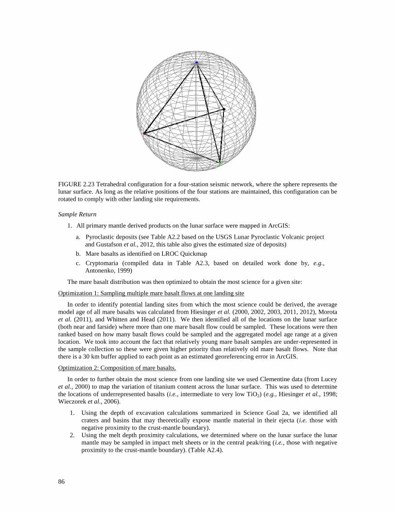
86
FIGURE 2.23 Tetrahedral configuration for a four-station seismic network, where the sphere represents the
lunar surface. As long as the relative positions of the four stations are maintained, this configuration can be
rotated to comply with other landing site requirements.
Sample Return
1. All primary mantle derived products on the lunar surface were mapped in ArcGIS:
a. Pyroclastic deposits (see Table A2.2 based on the USGS Lunar Pyroclastic Volcanic project
and Gustafson et al., 2012, this table also gives the estimated size of deposits)
b. Mare basalts as identified on LROC Quickmap
c. Cryptomaria (compiled data in Table A2.3, based on detailed work done by, e.g.,
Antonenko, 1999)
The mare basalt distribution was then optimized to obtain the most science for a given site:
Optimization 1: Sampling multiple mare basalt flows at one landing site
In order to identify potential landing sites from which the most science could be derived, the average
model age of all mare basalts was calculated from Hiesinger et al. (2000, 2002, 2003, 2011, 2012), Morota
et al. (2011), and Whitten and Head (2011). We then identified all of the locations on the lunar surface
(both near and farside) where more than one mare basalt flow could be sampled. These locations were then
ranked based on how many basalt flows could be sampled and the aggregated model age range at a given
location. We took into account the fact that relatively young mare basalt samples are under-represented in
the sample collection so these were given higher priority than relatively old mare basalt flows. Note that
there is a 30 km buffer applied to each point as an estimated georeferencing error in ArcGIS.
Optimization 2: Composition of mare basalts.
In order to further obtain the most science from one landing site we used Clementine data (from Lucey
et al., 2000) to map the variation of titanium content across the lunar surface. This was used to determine
the locations of underrepresented basalts (i.e., intermediate to very low TiO2) (e.g., Hiesinger et al., 1998;
Wieczorek et al., 2006).
1. Using the depth of excavation calculations summarized in Science Goal 2a, we identified all
craters and basins that may theoretically expose mantle material in their ejecta (i.e. those with
negative proximity to the crust-mantle boundary).
2. Using the melt depth proximity calculations, we determined where on the lunar surface the lunar
mantle may be sampled in impact melt sheets or in the central peak/ring (i.e., those with negative
proximity to the crust-mantle boundary). (Table A2.4).

87
3. LROC Quickmap was then used to visually determine whether those craters and basins do actually
preserve their central peaks or peak rings. For example, Imbrium basin was calculated to contain
mantle material in its central peak/ring however, it is not visible in LROC images as it is masked
by younger mare basalt flows, and thus the central uplift is not available for sampling.
4. The secondary target site data was then compared to the spectral profiler olivine detection data of
Yamamoto et al. (2010, 2012), which may indicate presence of troctolite/dunite at the surface.
(Table A2.5)
5. Finally, optimized primary target data was compared with secondary target site data, to select the
landing sites providing the most scientific opportunity.
As described in Science Goal 2a, the formation mechanism of rings and peak rings is highly debated.
Thus, craters or basins calculated to sample mantle material should be treated with caution. For example,
Imbrium and Serenitatis basins are considered to have sampled mantle, but Apollo 15 and 17 astronauts did
not obtain any samples of mantle material from them.
Suggested Landing Sites
In situ Geophysics
Due to the nature of requirements for geophysical methods, no specific landing sites are suggested, but
any set of geophysical landing sites chosen to address Science Goal 2b should maintain a tetrahedral
configuration (see Methodology, above).
Sample Return
Figure 2.24 shows everywhere on the lunar surface where primary target sites (mantle derived products)
might be sampled. Note that the pyroclastic deposits are of various sizes (from <1 to >49,000 km2).
Table A2.6 and Fig. A2.1 shows the results of Optimization 1. Optimization 2 then identified the
locations of underrepresented basalts at Mare Frigoris, northern and eastern Oceanus Procellarum, northern
Mare Imbrium, northern Mare Serenitatis, and SPA. Figure 2.25 shows the combination of Optimization 1
and Optimization 2 for mare basalts. Overlap with high priority Optimization 1 and Optimization 2 sites
occurs in northern and eastern Oceanus Procellarum, Mare Frigoris, NW Imbrium, proximal to Aristarchus
crater, and NW Mare Serenitatis.
Table A2.4 identifies all of those craters and basins that potentially sample mantle material in their
central uplifts (peaks/rings). From the calculations there are only three basins that have potentially sampled
mantle material in their ejecta blankets (South Pole-Aitken basin, Imbrium and Serenitatis). From
consultation with LROC Quickmap, the basins which potentially expose mantle material in their preserved
central uplifts are Apollo, Hertzsprung, Orientale, Nectaris, Moscoviense, Schrödinger, Amundsen-
Ganswindt and Poincare.
Conclusions
Figure 2.26 shows the final suggested landing sites, deduced by comparing primary and secondary
sample return target sites and identifying any overlaps. Since there are no specific geophysical locations
(c.f., Suggested Landing Sites) and only a configuration that must be maintained, any site chosen for
sample return should also contain a seismometer and, if appropriate, an LLR station.
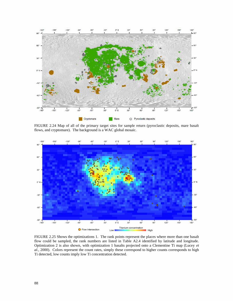
88
FIGURE 2.24 Map of all of the primary target sites for sample return (pyroclastic deposits, mare basalt
flows, and cryptomare). The background is a WAC global mosaic.
FIGURE 2.25 Shows the optimizations 1. The rank points represent the places where more than one basalt
flow could be sampled, the rank numbers are listed in Table A2.4 identified by latitude and longitude.
Optimization 2 is also shown, with optimization 1 basalts projected onto a Clementine Ti map (Lucey et
al., 2000). Colors represent the count rates, simply these correspond to higher counts corresponds to high
Ti detected, low counts imply low Ti concentration detected.

89
FIGURE 2.26 Shows the final landing site map for Science Goal 2b sample return. The highlighted craters
and basins are those within which there is the most overlap between primary and secondary target
lithologies. Background of WAC global mosaic.
SCIENCE GOAL 2C: DETERMINE THE SIZE, COMPOSITION, AND STATE (SOLID/LIQUID)
OF THE CORE OF THE MOON
Introduction
Despite more than three decades of remote sensing analyses, relatively little is known about the current
size, composition, and state of the lunar core. Besides generally verifying its existence, previous work
suggests that (1) the core is between 1–3% of the mass of the Moon and thus has a relatively small radius
(<500 km: e.g., Williams et al., 2001), (2) the core could be composed of pure Fe metal, Fe-FeS metal, or
Ti-rich silicates (e.g., Wieczorek and Zuber, 2002), and (3) the core is either partially or fully molten (e.g.,
Williams et al., 2001). Knowledge of the current characteristics of the core is an important consideration
for planetary differentiation and thermal evolution, especially because it provides fundamental constraints
on lunar formation hypotheses (Wieczorek et al., 2006). Therefore, addressing this Science Goal will also
provide information for Science Goal 2d.
Core size can be constrained through a variety of geophysical methods, including moment of inertia
measurements, lunar laser ranging (LLR), electromagnetic (EM) sounding, heat flow measurements, and
seismology. While each of these datasets independently provides particular information about the core,
they should be used together in order to reduce the non-uniqueness of calculated core size (e.g. moment of
inertia measures the distribution of mass, but it does not give detailed density structure and allows for
multiple fits to a single data point).
The concentration of siderophile (‗iron-loving‘) elements in the crust and mantle can also provide
information on differentiation and core formation (e.g., Righter, 2002). If the crust and mantle are
relatively depleted in siderophile elements, then it is likely that the Moon underwent some level of core
formation. However, while geochemical data are useful in determining the possible existence of a core,
there is not one particular sample type that addresses its current size, composition and state. Therefore,
landing sites for sample return are not addressed in this Science Goal.

90
Background
Size of the lunar core
A summary of published data on possible core sizes is shown in Table 2.3. Information on the size of
the lunar core was obtained by Apollo-era seismic analyses (e.g., Nakamura et al., 1974; Sellers, 1992;
Weber et al., 2011), EM sounding from both lunar surface and low-orbit measurements (e.g., Dyal et al.,
1976; Hood et al., 1982; 1999), moment of inertia (Konopliv et al., 1998), and LLR (e.g., Williams et al.,
2001). Some authors have also used petrologic, thermal, and geophysical constraints to model potential
core sizes (Binder, 1980; Mueller et al., 1988; Kuskov et al., 2002). In all, these analyses suggest the
existence of a lunar core between 150 and 500 km in radius.
A few caveats are required to interpret these size ranges. First, many publications indicate that a core is
permissible but not required to fit the available data (Dyal et al., 1976; Goins et al., 1981b; Hobbs et al.,
1983; Sellers, 1992; Konopliv et al., 1998; Wieczorek and Zuber, 2002). As such, much of the early EM
sounding and seismic work should be viewed as maximum permissible core sizes rather than best estimates
of core size. Secondly, inferences about core size are highly dependent on the modeled core composition,
such that pure Fe-metal core sizes are smaller than Fe-FeS metal cores, which are in turn smaller than Ti-
rich silicate cores (Wieczorek and Zuber, 2002). This is especially true for EM sounding data because of
the conductivity differences between potential metal and silicate compositions; larger cores with lower
conductivity (i.e., Ti-rich basalts) can fit the data as well as smaller cores with higher conductivity (i.e.,
pure Fe or Fe-rich metal). Higher-resolution geophysical data have the potential to reduce the non-
uniqueness of these solutions.
Composition of the lunar core
Existing data on the composition of the lunar core suggest two possible end-members: metallic (pure
Fe, FeS, Fe-FeS eutectic, or Fe-FeS-C alloy: Wieczorek et al., 2006) or dense Ti-rich silicate (Hess and
Parmentier, 1995; Wieczorek and Zuber, 2002). Most of the geophysical data are non-unique with respect
to core composition, and either metal or silicate cores are possible (Wieczorek and Zuber, 2002; Kuskov et
al., 2002; Wieczorek et al., 2006). However, certain datasets either require or exclude one of the possible
end-members. Paleomagnetic data from returned Apollo samples strongly suggest the presence of a
metallic core (e.g., Cisowski, 1983; Shea et al., 2012), and this contention is supported by geochemical
modelling (Buck and Toksöz, 1980) and highly-siderophile element depletion in the lunar mantle (Righter,
2002). Hafnium-tungsten (Hf-W) systematics also indicate a metallic core, but by a different formation
process than the other terrestrial planets (i.e., giant impact as opposed to accretion) (Kleine et al., 2002). If
the Moon does contain a metallic core, it is unlikely to be pure Fe, but rather a Fe-FeS eutectic composition
(Stevenson and Yoder, 1981; Khan and Mosegaard, 2001; Weber et al., 2011). It is also likely that Fe
would entrain C to the core during core formation as has been postulated for Earth (Hirayama et al., 1993;
Wieczorek et al., 2006).
Alternatively, models of global cumulate overturn suggest that ilmenite-rich material sank toward the
center of the Moon early in lunar history (c.f., Science Goal 2b), either blanketing an existing metallic core
or creating a dense silicate core (Hess and Parmentier, 1995; Wieczorek and Zuber, 2002; de Vries et al.,
2010). There is evidence that a silicate core could theoretically be a strong enough conductor to produce a
lunar dynamo (Wieczorek et al., 2006), but there is some debate as to whether or not it could remain
molten until the present, as required by the LLR data (Hood et al., 1999; Wieczorek and Zuber, 2002).
Certain geophysical models are also best fit by a dense silicate core (Khan and Mosegaard, 2001).
Previous work has shown either of the two compositional end-members to be viable possibilities, with
more data required to discriminate between them.
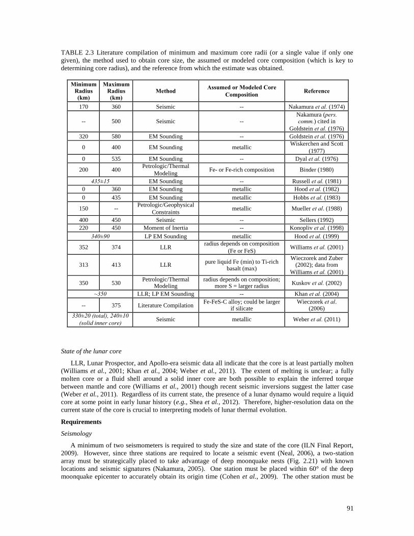
91
TABLE 2.3 Literature compilation of minimum and maximum core radii (or a single value if only one
given), the method used to obtain core size, the assumed or modeled core composition (which is key to
determining core radius), and the reference from which the estimate was obtained.
Minimum Radius (km)
Maximum Radius (km)
Method Assumed or Modeled Core
Composition Reference
170 360 Seismic -- Nakamura et al. (1974)
-- 500 Seismic -- Nakamura (pers. comm.) cited in
Goldstein et al. (1976)
320 580 EM Sounding -- Goldstein et al. (1976)
0 400 EM Sounding metallic Wiskerchen and Scott
(1977)
0 535 EM Sounding -- Dyal et al. (1976)
200 400 Petrologic/Thermal
Modeling Fe- or Fe-rich composition Binder (1980)
435±15 EM Sounding -- Russell et al. (1981)
0 360 EM Sounding metallic Hood et al. (1982)
0 435 EM Sounding metallic Hobbs et al. (1983)
150 -- Petrologic/Geophysical
Constraints metallic Mueller et al. (1988)
400 450 Seismic -- Sellers (1992)
220 450 Moment of Inertia -- Konopliv et al. (1998)
340±90 LP EM Sounding metallic Hood et al. (1999)
352 374 LLR radius depends on composition
(Fe or FeS) Williams et al. (2001)
313 413 LLR pure liquid Fe (min) to Ti-rich
basalt (max)
Wieczorek and Zuber (2002); data from
Williams et al. (2001)
350 530 Petrologic/Thermal
Modeling radius depends on composition;
more S = larger radius Kuskov et al. (2002)
~350 LLR; LP EM Sounding -- Khan et al. (2004)
-- 375 Literature Compilation Fe-FeS-C alloy; could be larger
if silicate Wieczorek et al.
(2006)
330±20 (total), 240±10
(solid inner core) Seismic metallic Weber et al. (2011)
State of the lunar core
LLR, Lunar Prospector, and Apollo-era seismic data all indicate that the core is at least partially molten
(Williams et al., 2001; Khan et al., 2004; Weber et al., 2011). The extent of melting is unclear; a fully
molten core or a fluid shell around a solid inner core are both possible to explain the inferred torque
between mantle and core (Williams et al., 2001) though recent seismic inversions suggest the latter case
(Weber et al., 2011). Regardless of its current state, the presence of a lunar dynamo would require a liquid
core at some point in early lunar history (e.g., Shea et al., 2012). Therefore, higher-resolution data on the
current state of the core is crucial to interpreting models of lunar thermal evolution.
Requirements
Seismology
A minimum of two seismometers is required to study the size and state of the core (ILN Final Report,
2009). However, since three stations are required to locate a seismic event (Neal, 2006), a two-station
array must be strategically placed to take advantage of deep moonquake nests (Fig. 2.21) with known
locations and seismic signatures (Nakamura, 2005). One station must be placed within 60° of the deep
moonquake epicenter to accurately obtain its origin time (Cohen et al., 2009). The other station must be

92
placed near the antipode of the seismic source to record waves that have travelled through the deep interior,
which we define as being within 120 km of the geometric center of the Moon (Fig. 2.27). One DMQ nest,
termed A33, has the advantage of being located on the farside with a nearside antipodal point (Goins et al.,
1981b). The majority of other nests, however, would require a station on the farside.
FIGURE 2.27 Geometry of the two-station set-up (discussed in text) that will elucidate the size and
physical state of the lunar core. Here, the Moon is approximated to be a sphere with radius R. Z is the
depth of the deep moonquake source. Station 1 would be placed within a distance S1 from the antipode,
and station 2 will be placed within a distance S2 from the epicenter. a is conservatively taken to be half of
the most recent estimates for an inner core radius of 240 km (Weber et al., 2011).
Lunar Laser Ranging (LLR)
Additional stations to the current LLR retroreflector network will provide the deformation properties,
geometries, and depths of major compositional and phase change interfaces (i.e. mantle-outer core, outer
core-inner core) of the lunar interior (Williams et al., 2010). These improvements require an increase in
the three-dimensional coverage of the retroreflector network to more accurately record the three-axis
physical lunar libration. The LLR arrays are also required to be on the nearside, and positioned within
regions constantly visible from Earth during the full libration period. Geophysical landing site selection
(LSS) will be partially driven by those visible locations that would make the most improvement to the
current retroreflector network.
Heat Flow
Heat flow measurements can provide constraints on the size and thermal state of the core. Although it
is not the main driver for geophysical landing site selection to address Science Goal 2c, it is still important
to consider if a location is suitable for making heat flow measurements. For specific requirements of global
heat flow studies, see Science Goal 2d where it is a main driver for geophysical landing site selection.
EM Sounding
EM sounding can provide constraints on the size, composition and thermal state of the core. This can
be done with the Magnetotellurics (MT) method at a single site with no restrictions on its location. Thus, it
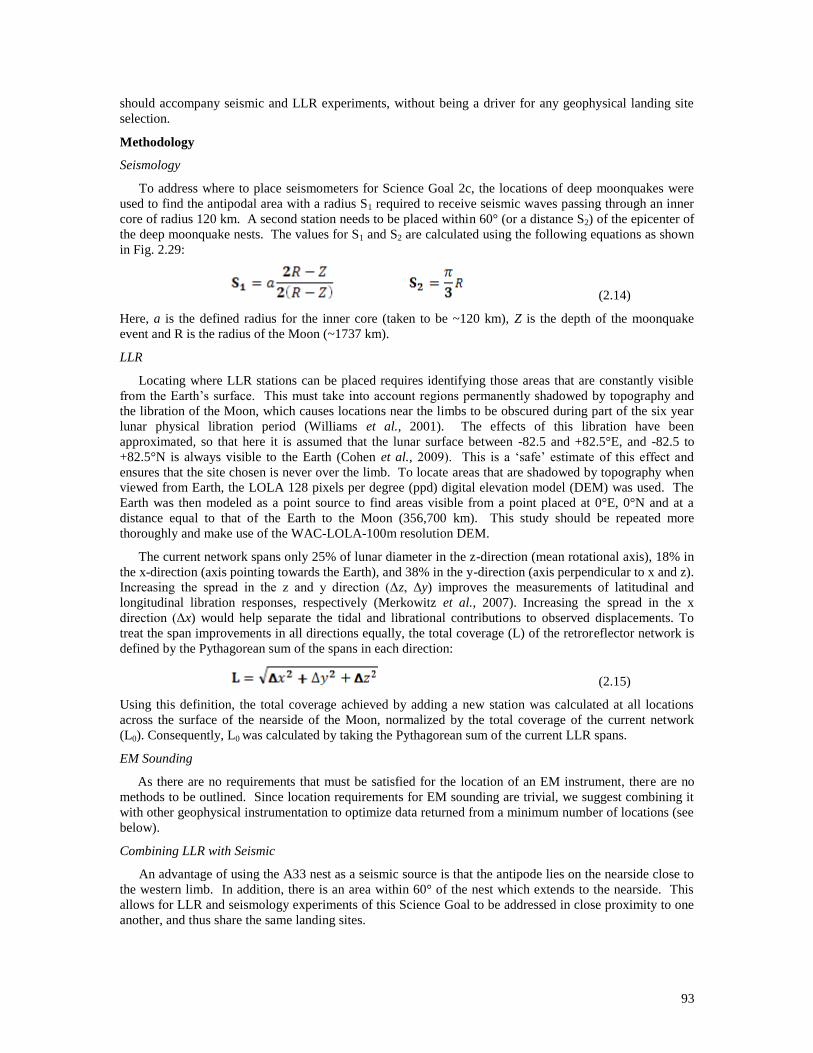
93
should accompany seismic and LLR experiments, without being a driver for any geophysical landing site
selection.
Methodology
Seismology
To address where to place seismometers for Science Goal 2c, the locations of deep moonquakes were
used to find the antipodal area with a radius S1 required to receive seismic waves passing through an inner
core of radius 120 km. A second station needs to be placed within 60° (or a distance S2) of the epicenter of
the deep moonquake nests. The values for S1 and S2 are calculated using the following equations as shown
in Fig. 2.29:
(2.14)
Here, a is the defined radius for the inner core (taken to be ~120 km), Z is the depth of the moonquake
event and R is the radius of the Moon (~1737 km).
LLR
Locating where LLR stations can be placed requires identifying those areas that are constantly visible
from the Earth‘s surface. This must take into account regions permanently shadowed by topography and
the libration of the Moon, which causes locations near the limbs to be obscured during part of the six year
lunar physical libration period (Williams et al., 2001). The effects of this libration have been
approximated, so that here it is assumed that the lunar surface between -82.5 and +82.5°E, and -82.5 to
+82.5°N is always visible to the Earth (Cohen et al., 2009). This is a ‗safe‘ estimate of this effect and
ensures that the site chosen is never over the limb. To locate areas that are shadowed by topography when
viewed from Earth, the LOLA 128 pixels per degree (ppd) digital elevation model (DEM) was used. The
Earth was then modeled as a point source to find areas visible from a point placed at 0°E, 0°N and at a
distance equal to that of the Earth to the Moon (356,700 km). This study should be repeated more
thoroughly and make use of the WAC-LOLA-100m resolution DEM.
The current network spans only 25% of lunar diameter in the z-direction (mean rotational axis), 18% in
the x-direction (axis pointing towards the Earth), and 38% in the y-direction (axis perpendicular to x and z).
Increasing the spread in the z and y direction (Δz, Δy) improves the measurements of latitudinal and
longitudinal libration responses, respectively (Merkowitz et al., 2007). Increasing the spread in the x
direction (Δx) would help separate the tidal and librational contributions to observed displacements. To
treat the span improvements in all directions equally, the total coverage (L) of the retroreflector network is
defined by the Pythagorean sum of the spans in each direction:
(2.15)
Using this definition, the total coverage achieved by adding a new station was calculated at all locations
across the surface of the nearside of the Moon, normalized by the total coverage of the current network
(L0). Consequently, L0 was calculated by taking the Pythagorean sum of the current LLR spans.
EM Sounding
As there are no requirements that must be satisfied for the location of an EM instrument, there are no
methods to be outlined. Since location requirements for EM sounding are trivial, we suggest combining it
with other geophysical instrumentation to optimize data returned from a minimum number of locations (see
below).
Combining LLR with Seismic
An advantage of using the A33 nest as a seismic source is that the antipode lies on the nearside close to
the western limb. In addition, there is an area within 60° of the nest which extends to the nearside. This
allows for LLR and seismology experiments of this Science Goal to be addressed in close proximity to one
another, and thus share the same landing sites.

94
Combining LLR, Seismic, and Heat Flow
Once requirements for the driver of geophysical landing site selection are met, extra requirements can
be placed to see if there are locations that satisfy the requirements for LLR, seismic and heat flow
instruments simultaneously. The requirements and methods for mapping landing sites suitable for heat
flow measurements are discussed in detail in Science Goal 2d, where it is a primary driver for geophysical
landing site selection.
Suggested Landing Sites
Seismology
Using information on current moonquake nests and Equation 2.14, circles can be plotted showing
potential seismic station placement (Fig. 2.28). The A33 moonquake nest was used as an example, as it has
station pairs that can be located on the nearside, meaning sites can be combined with LLR sites.
LLR
Landing sites for placing LLR stations must avoid areas never or not always visible from the Earth‘s
surface due to apparent lunar libration. These sites are plotted in Fig. 2.29.
Figure 2.30 shows the comparative improvement in the current LLR retroreflector network coverage
that can be achieved by placing an additional retroreflector at a specific location, taking into account the x,
y, and z span of the network. The map shows that placing LLR stations at the limbs and closer to the South
Pole than the current stations significantly improves the LLR network coverage. The dark blue area in the
center of the map shows the area for which placement of an additional retroreflector would not improve the
current LLR coverage; red shows areas which would best improve the current LLR network.
FIGURE 2.28 Location of known moonquake nests and the areas within which seismometers can be placed
to gather information regarding the core. The A33 nest and antipode are highlighted as this nest offers the
opportunity to combine LLR and seismology experiments within the same landing site, as discussed in the
text. Circles are projected onto the IAU Moon 2000 sphere.

95
FIGURE 2.29 Map showing areas that are never or not always visible from Earth (red). LLR stations can
be placed in any non-red location (nearside only). Current LLR retroreflector stations are shown. The
background is the WAC Global Mosaic.

96
FIGURE 2.30 Map showing how placing a retroreflector at a specific location can improve the x, y, and z
coverage of the current LLR network. Axes are shown on the bottom-left, with x pointing out of the page.
Dark grey represents the areas which do not have a direct line of sight with Earth at all times during the 6
year lunar physical libration period. Blue regions represent minimal to no improvement relative to the
current network configuration, while yellow to red regions are the best locations for an additional
retroreflector.
Combining LLR with Seismic
LLR and seismic requirements are the primary drivers for Science Goal 2c landing site selection; Figs.
2.28 and 2.30 show all the locations where these geophysical analyses can be placed on the lunar surface.
They have been combined in the final geophysical and overall maps for Science Concept 2, which also
consider the tetrahedral requirement for a global seismic network. For the purposes of Science Goal 2c,
any seismic station placed on the nearside should include an LLR retroreflector, but the choice of the deep
moonquake nest used to probe the core (Fig. 2.28) will determine where that station should be placed. A
specific example is shown in the A33 Case Study.
Combining LLR, Seismic, and Heat Flow
By combining heat flow with other geophysical experiments, much of the surface becomes ruled out of
the landing site selection process. However, there are still potential landing sites remaining within the A33
nest and its antipode (Fig. 2.28), and the addition of two LLR stations would represent a significant
increase in the current extent of the network. Figure 2.31 shows the same information as Fig. 2.28 but
displays all the known deep moonquake nests. This shows that only three farside moonquake nests are
suitable for the combined package of heat flow, LLR, and seismic experiments, assuming that only two

97
packages containing all three experiments are used. However, there are plenty of available sites should a
nearside moonquake nest with a farside antipode be chosen. Any of these antipodes would be suitable for
the study of the lunar core, providing that the second seismometer is placed within 60° of the moonquake
nest. Some of these moonquake nests are well constrained using the currently available data, whilst some
are not; refer to Nakamura (2005) for the location errors for each moonquake nest.

98
FIG
UR
E 2
.31
Map
sh
ow
ing
th
e sa
me
dat
a as
Fig
. 2
.30 a
pp
lied
to
all
kn
ow
n m
oon
qu
ake
nes
ts.
Th
is i
s to
hig
hli
gh
t th
at t
he
A3
3 m
oo
nqu
ake
nes
t is
no
t th
e o
nly
dee
p m
oo
nq
uak
e n
est
that
co
uld
be
use
d,
bu
t th
at i
t is
on
e o
f th
e fe
w k
no
wn
moo
nqu
akes
th
at r
egu
larl
y o
ccu
r o
n t
he
fars
ide.

99
SCIENCE GOAL 2D: CHARACTERIZE THE THERMAL STATE OF THE INTERIOR AND
ELUCIDATE THE WORKINGS OF THE PLANETARY HEAT ENGINE
Introduction
Many geological and geochemical processes are driven by the removal of heat from the interior. Heat
sources include energy accumulated during initial accretion and subsequent impacts, radioactive decay,
tidal forcing, insolation, and bond energy release from chemical or phase changes. These energy sources
either directly generate heat (i.e., impact heating, latent heat, exothermic chemical processes, radioactivity)
or produce material transport (i.e., thermal/chemical convection, mechanical stirring from giant impacts,
tidal deformation) that leads to viscous heat dissipation from internal friction or ohmic heat dissipation of
currents generated during the dynamo process. A variety of factors such as energy budget, size and
geometry of internal boundaries (i.e., core mantle boundary (CMB) oblateness, crustal asymmetry),
chemistry, composition, distribution of radiogenic elements, and orbital evolution can affect the thermal
evolution of a planetary body.
The ways in which a planetary body removes heat dictate the physical and chemical evolution of its
interior and its current state. Thus we need not only to study its present structure and composition, but also
to understand the evolution of the planetary heat engine. The intimate link between thermodynamics and
geology means that studies of thermal history require concurrent analyses of all aspects of lunar science
affected by thermal processing.
Samples returned for Science Concept 1 will gauge the early impact flux of the Moon and provide
insight into heat provided to the interior. Science Goal 2b, Science Concept 3 (Science Goals 3a and 3b),
and Science Concept 5 (Science Goals 5a, 5b, and 5d) have proposed to sample various mare basalt flows
within and outside the PKT. Data obtained from those samples will address the early cooling history of the
Moon, in particular the evolution of basalt — and therefore upper mantle — chemistry and the distribution
of KREEP through time. Thus, sample return for Science Concept 1, Science Goal 2b, Science Concept 3,
and Science Concept 5 will also contribute to Science Goal 2d. In addition, geophysical data obtained for
Science Goal 2a, 2b, and 2c will contribute greatly to our understanding of Science Goal 2d.
Background
It is hypothesized that the lunar magma ocean (LMO) occurred shortly after the giant impact that
formed the Moon (Shearer et al., 2006; c.f., General Background). The depth of this LMO constrains the
initial conditions of the lunar interior and its subsequent thermal evolution. This evolution is also affected
by the primary anorthositic crust formed in the LMO, which acts as an insulating thermal boundary layer
(Ziethe et al., 2009). The core formation process advected heat out of the interior through material
transport, likely producing an adiabatic temperature profile (Konrad and Spohn, 1997). The convection of
a possible fluid metallic core early in lunar history and the generation of a core dynamo (Stevenson, 1983;
Stegman et al., 2003) put constraints on the rate at which heat was produced and removed from the core.
Paleomagnetic data suggest a relatively strong dynamo had been active and peaked between 4.0–3.8 Ga
(Fuller, 1974; Collinson et al., 1977; Cisowski, 1983; Garrick-Bethell et al., 2009; Shea et al., 2012). The
strength and persistence of the recorded magnetic field is difficult to explain with current thermal evolution
models due to the lack of adequate energy during late accretion, although the energy budget of the core
may have been expanded by later modification (LeBars et al., 2011; Dwyer et al., 2011). The subsequent
magmatic evolution until 1.2 Ga (Hiesinger et al., 2003) was characterized by the emergence of basaltic
lava, which flooded large impact basins. Younger eruptions are difficult to explain with current models
from an energy perspective because of the small size of the Moon and its inevitably rapid cooling;
however, insulation by the crust and megaregolith combined with added heat energy could have curbed its
secular cooling (Ziethe et al., 2009). Factors such as meteorite impact flux, orbital evolution of tidal
forcing, distribution of heat-producing elements, and crustal thickness variations affect this evolution to the
current thermal state.
Present thermal state
Current global heat flux measurements are essential to assess the past and present thermal state of the
Moon by providing both spatial and temporal boundary conditions for thermal models. Previous
measurements of heat flow were taken during Apollo 15 and 17 (Langseth et al., 1976) and yielded values
of 21 and 14 mW/m2, respectively. Unfortunately, both experiments suffered from a number of possible

100
interferences and were placed along terrane boundaries, making their representation of the lunar global heat
flux questionable (e.g., Conel and Morton, 1975; Warren and Rasmussen, 1987; Kiefer, 2012). The
baseline measurement of any study of the planetary heat engine is an assessment of the current global heat
flow. Thus, it is absolutely essential to obtain new heat flow measurements in each terrane and avoid
locations where heat flow would be anomalous (c.f., Requirements-Geophysical).
Once boundary conditions are obtained (i.e., the heat flow distribution at the surface), the extension of
the lunar thermal gradient requires knowledge of density and compositional stratification, since
temperature, pressure, density and composition must be inverted for simultaneously (Dziewonski and
Anderson, 1981). The thermal boundary layer (a layer in which the thermal state changes rapidly in order
to match the boundary condition imposed by the surface) can be well approximated by a conductive
temperature profile (Tcond(z)), and can be calculated by integrating the steady-state heat equation (Turcotte
and Schubert, 2002, p. 250):
(2.16)
with outer boundary conditions (i.e. and T at z = 0) determined by the heat flow experiments. Values
of thermal conductivity (k), density (), and radiogenic heat production rate (H) vary with depth (z). These
variables need to be determined using EM sounding, seismology and geochemical studies. The controlling
factor for the geotherm at a particular location is H, since it can vary by many orders of magnitude
depending on the quantity of various radioactive elements (Table 2.4) in the crust. Large lateral variations
of H are expected due to a concentration of radioactive elements in the Procellarum KREEP Terrane (PKT)
(Jolliff et al., 2000). The depth extent of this conductive profile will also vary laterally because of
variations in crustal thickness (Wieczorek et al., 2006). Thus, conductive geotherms will vary globally and
must be studied at multiple locations to determine the global thermal profile.
TABLE 2.4 Heat production rate and half-life ( ½) of various isotopes of elements relevant for the Moon.
The actual radiogenic heat production rate in a volume will depend on the total concentration of each
element (data from Turcotte and Schubert, 2002).
Isotope H (W/kg) τ1/2 (yr)
238U 9.46 × 10
-5 4.47 × 10
9
235U 5.69 × 10
-4 7.04 × 10
8
232Th 2.64 × 10
-5 1.40 × 10
10
40K 2.92 × 10
-5 1.25 × 10
9
Near the bottom of the thermal boundary layer (i.e., the upper mantle), the temperature profile becomes
approximately adiabatic (Konrad and Spohn, 1997). This adiabatic temperature profile (Tadia(z)) can be
obtained through the joint integration of variables (e.g., density and composition) using Equation 2.17
(Turcotte and Schubert, 2002, p. 340):
(2.17)
Cp is the specific heat capacity at constant pressure and V is the volumetric thermal expansion coefficient
of the material (both of which depend on the pressure, temperature and chemical composition) and g is the
gravitational acceleration at that depth, which depends on the radial density profile. A global passive
seismic network along with EM sounding can be employed (c.f., Science Goal 2b) to determine the density
and compositional stratification of the mantle and its lateral heterogeneity.

101
Any discontinuity in density or composition within the adiabatic profile can complicate thermal models
by creating boundary layers that stall advective heat transport (Turcotte and Schubert, 2002). This can lead
to major differences in geotherms by assuming that a conductive layer within the adiabatic region acts to
insulate the interior (Fig. 2.32).
The size and state of the core controls the inner boundary conditions for the temperature profile (i.e.,
heat flux and temperature at the CMB, its lateral variations, and the geometry of the CMB). The existence
of an inner core along with solidus temperatures of probable lower mantle chemical compositions can also
provide thermodynamic constraints. These constraints can elucidate the existence and thickness of an inner
thermal boundary layer that also adopts a conductive profile. To probe these properties, a combination of
seismology, LLR and EM sounding must be used (c.f., Science Goal 2c).
Figure 2.32 Possible one-dimensional temperature profiles for a planetary interior. Boundary conditions
for T, dT/dz at the surface and CMB constrain the minimum and maximum temperature of the profile, and
a compositional/density discontinuity changes the overall shape.
Thermal history
Three important heat sources are considered when modeling lunar thermal evolution: energy from
accretion, energy from impacts, and long-lived radioactive isotopes (Wieczorek et al., 2006). Energy from
accretion affects the primary thermal state of the whole Moon during formation and governs how much
initial melting occurs (Melosh, 1990). Energy from impacts has important consequences for the outer
layers of the Moon and may have some influence on the location of volcanic provinces (Cintala and Grieve,
1998; Elkins-Tanton et al., 2004). Long-lived radioactive isotopes affect the entire Moon and are a major
driver for volcanism (Wieczorek and Phillips, 2000). A number of models have been created to address the
early thermal state of the Moon, ranging from purely conductive to purely convective with some level of
melting and/or melt migration (for more details regarding these models, the reader is directed to Tables
4.10 and 4.11 of Shearer et al. (2006)). However, a lack of new data on these issues has led to a stagnation
in thermal model development.
Data from the Apollo missions had a profound impact on our understanding of the thermal evolution of
the Moon. The favored hypothesis for lunar origin is through the accretion of material that was flung into
Earth orbit from a giant impact (Canup, 2004b; c.f., General Background). Some models suggest that
accretion of this material was rapid, on the order of 100 years (Pritchard and Stevenson, 2000), leading to

102
an initially fully molten Moon. However, a lack of large-scale global contractional features have led others
to postulate that the early Moon had a cold interior (e.g., Solomon and Chaiken, 1976). The initial state of
the interior is a topic of much debate and is fundamental to our understanding of thermal evolution.
Samples from the Apollo missions indicate that large scale melting did occur early in lunar history (e.g.,
Taylor and Jakes, 1974; Warren, 1985) and is attributed to rapid accretion from an impact origin. The
depth of this melting, known as the lunar magma ocean (LMO; c.f., General Background), is largely
unknown (ranging from 200–1000 km or more; Solomon and Chaiken, 1976; Nakamura, 1983) and
debated but has significant ramifications for thermal evolution. For instance, if the LMO extended the
entire radius of the Moon, it would have a much longer cooling history than an LMO that was only a few
hundred kilometers deep.
The crystallization sequence of the LMO (Taylor and Jakes, 1974) and mantle mixing as suggested by
mare and pyroclastic chemistries (Hughes et al., 1988; Ryder, 1991) have led to the hypothesis of cumulate
overturn. Dense, Fe- and Ti-rich mineral cumulates were formed in the latest stages of the LMO, leaving
an inverse density sequence that would overturn due to gravitational instability (Ringwood and Kesson,
1976; Elkins-Tanton et al., 2002; c.f., General Background), releasing energy in the process. In addition,
incompatible elements (particularly potassium, rare earth elements, and phosphorus (KREEP)) are the last
to crystallize and the distribution of this layer, known as urKREEP, is particularly important for thermal
evolution due its relatively high concentration of radioactive elements (Meyer et al., 1971). At this point it
is unknown if this layer was a global phenomenon, but surface observations suggest a high concentration
on the nearside (Procellarum KREEP Terrane (PKT); Jolliff et al., 2000). An asymmetric distribution of
KREEP would lead to an asymmetric distribution of heat flux, further complicating thermal models. In
addition, the asymmetric nature of crustal thickness (Ohtake et al, 2012; c.f., Science Goal 2a) would act as
a heterogeneous lid, affecting heat flux. It is believed that this KREEP concentration is one of the factors
leading to the asymmetric distribution of mare volcanism (Wieczorek and Phillips, 2000).
The paucity of geophysical data regarding the interior has led scientists to unravel the thermal history
through Apollo samples. Magmatic processes such as picritic glasses and mare volcanism provide clues to
the thermal state of various depths in the Moon at various points in time. Picritic glasses have a large range
of titanium concentrations and indicate source regions of 200 km or more (Wieczorek et al., 2006; c.f.,
Science Goal 2b and Science Concept 5). Mare basalts also have a wide range of compositions (BVSP,
1981; c.f., Science Goal 2b and Science Concept 5), indicating a heterogeneous source region at depths of
100–500 km. Mare volcanism reached a peak at 3.6–3.9 Ga, with the majority of basalt erupting between
2.5–3.9 Ga (Head, 1976). However, there is evidence for recent (~1.1 Ga; Hiesinger et al., 2011) and very
old (cryptomare, >3.9 Ga; Antonenko, 1999) mare volcanism, although they are less prevalent (or obscured
by regolith in the case of cryptomare). Thickness estimates for these magmatic episodes range from a few
hundred meters (De Hon and Waskom, 1976) to 4.5 kilometers (Head and Wilson, 1992), with individual
flows on the order of tens to hundreds of meters thick (Hiesinger et al., 2002; Robinson et al., 2012).
However, much work remains to be done in characterizing flow unit thicknesses and basalt volumes
globally, as this will provide important constraints on heat flux and secular cooling.
Volcanic processes record not only the thermal state of the magmatic source region, but also the
magnetic field environment at the time of emplacement, revealing the energy state of a possible core
dynamo. Thus, it is critical to conduct geologic and paleomagnetic studies of lithologies that could record
the presence of an early dynamo.
Paleomagnetic studies
Rock samples are used to gauge the timing, intensity, and orientation of the purported dynamo. The
Moon would have cooled faster than larger planetary bodies due to its small size (de Pater and Lissauer,
2010), thus making it more likely that a dynamo would have operated early in its history rather than later.
Therefore, rocks containing magnetic minerals (i.e. iron oxides, iron-titanium oxides) that formed early in
lunar history would have retained a signature of this dynamo. The lithologies that will be considered for
sample return are mare basalt flows older than 3.0 Ga and impact melt sheets of basins that are Imbrian or
older (≥ 3.2 Ga), as previous studies suggests any lunar dynamo would have operated during this time.
Rocks that retain a magnetic signature are known to have natural remnant magnetization (Butler, 2004).
This means that magnetic minerals (i.e. iron oxides) within the rock have cooled below their Curie

103
temperature (the temperature at which magnetic minerals hold a magnetization) in the presence of a
magnetic field, even though there may not be one currently. Because ancient (≥ 3.2 Ga) lunar rocks have a
natural remnant magnetization, albeit weak, it has been postulated that this magnetization was recorded in
the presence of a lunar dynamo (e.g. Collinson et al., 1977; Runcorn, 1994; Garrick-Bethell and Weiss,
2007a; Garrick-Bethell et al., 2009). Seismic (Weber et al., 2011) and LLR (Williams et al., 2001; Khan et
al., 2004) detections of a small liquid outer core support the existence of a lunar dynamo early in lunar
history.
Various lunar samples returned by the Apollo missions have been analyzed by paleomagnetic studies
(e.g. Fuller, 1974; Collinson et al. 1977; Cisowski, 1983; Runcorn, 1994). However, a reanalysis of the
data by Lawrence et al. (2008) showed the results obtained up to that point should not be considered
scientifically robust due to uncertainties and problems with the method used. Since then, more reliable
paleomagnetic measurements place dynamo activity at 4.2 Ga (Garrick-Bethell et al., 2009; Shea et al.,
2012) and 3.6 Ga (Suavet et al., 2012) (Fig. 2.33). Since there are no rock samples older than 4.2 Ga that
can be used for paleomagnetic studies, it is unknown when the dynamo would have begun operating. Due
to a lack of data and conflicting measurements from Tikoo et al. (2012a, 2012b) and Cournède et al.
(2012), it is also unclear when this dynamo would have shut down.
FIGURE 2.33 Paleomagnetic intensities of Apollo samples. Note that for many ages there is only one data
point, which is suboptimal for paleomagnetic studies.
Central magnetic anomalies
Another way to constrain the strength and timing of the lunar core dynamo is through surface studies of
central magnetic anomalies. The central magnetic anomalies are magnetic peaks or troughs near the center
of large impact basins. They are proposed to be associated with thermal remanent magnetization of impact
melt pools that had subsequently cooled below the Curie temperature and retained an ambient, steady state
magnetic field (Halekas et al., 2003; Hood and Halekas, 2010; Hood, 2011; Richmond and Hood, 2012).
Since only a core dynamo can produce a magnetic field that lasts longer than the cooling timescale of the

104
melt rock, and basin age provides the timing of the magnetization, a surface study of these magnetic
anomalies with a magnetometer traversal can provide the timing, orientation and energy state of the
possible lunar dynamo (Halekas et al., 2003). A survey of the basins that have these central magnetic
anomalies compared to their relative ages paints a picture of the lunar dynamo that is in rough agreement
with paleomagnetic studies (Fig. 2.34). A combination of surface magnetometer surveys and sample return
studies at sites of interest is required to determine the exact state of the dynamo at particular times in lunar
history.
FIGURE 2.34 Basins, Pre-Nectarian to Imbrian in age, showing the temporal distribution of central
magnetic anomaly signatures. Basins in the same column are in the same age class as defined by Wilhelms
(1987). (Anomalies identified by Halekas et al., 2003; Hood and Halekas, 2010; Hood, 2011; Richmond
and Hood 2012).
Important Geologic Features for Sample Return
Sinuous rilles
Sinuous rilles are meandering channels common on the lunar surface (Schubert et al., 1970). They are
proposed to have formed either as collapsed lava tubes (e.g., Greeley, 1971), lava channels with levees that
formed in existing depressions (e.g., Spudis et al., 1988), or lava channels that cut into a pre-existing
substrate due to thermal erosion (Hulme, 1973; 1982). A sinuous rille (Hadley) was visited by the Apollo
15 astronauts and was found to contain pristine, bedded mare in the upper walls of the rille (Figs. 2.35–
2.37; NASA, 1972). Though the astronauts did not descend into the rille itself, descriptions of rille wall
slope suggest an average of 25–30o (NASA, 1972), and photographic analyses of rilles suggest there are
numerous shallow entry points that sampling missions could exploit (Fig. 2.35).
Floor fractured craters
Floor-fractured craters have previously been catalogued by Science Concept 5 and are considered to
represent pre-mare impact craters that were modified and uplifted during mare flooding (Schultz, 1976).
While the fractures themselves may have been activated multiple times and may therefore expose mare
flow units, they may also potentially have been exploited as magma conduits or dikes (Schultz, 1976). It is
therefore unclear whether the appropriate samples for paleomagnetic studies (i.e., multiple, pristine,
exposed flow units) would be exposed at the surface. However, if they are indeed magma conduits or

105
dikes, it is likely that they would be magnetized in an active core dynamo, and thus are included as
potential sampling sites.
FIGURE 2.35 Apollo 15 Mission Photographs and Photogeologic Interpretation of Hadley Rille. (A)
Regional view of the Apollo 15 landing site, taken from the Lunar Module (LM) as it descended to the
surface. The dashed red circle outlines a potential shallow access point for the rille, and the red inset box
indicates the area of detail in B and C. A scale bar is not shown, as it varies across the photograph, but the
average rille width is ~1km. (B) Cropped photograph with elevated contrast and decreased brightness to
show stratigraphic detail of Hadley Rille. (C) Photogeologic interpretation of B, with regolith-covered
mare surface, zones of potential mare outcrops, and talus pile in rille center.
FIGURE 2.36 Cross-section of Hadley Rille area investigated by Apollo 15 astronauts (W to SW of landing
site). The regolith thickness gradually decreases towards the edge of the rille; coherent bedrock is exposed
for a number of meters below the rille edge but gives way to talus and regolith material with depth. Note

106
that the mare basalt itself is not thought to extend significantly below the edge of its exposure. Modified
from the Apollo 15 Preliminary Science Report (NASA, 1972).
FIGURE 2.37 Mission photograph from Apollo 15 showing coherently bedded mare flow units in the
western wall of Hadley Rille. This outcrop is ~30 m below the edge of the rille and ~8 m thick. Coherent
flow units such as these are appropriate potential sampling sites for paleomagnetism studies.
Requirements
In situ Geophysics
The use of geophysical measurements will provide a complete density, conductivity, and thermal cross-
section, thus helping to elucidate the thermal state of the interior and illuminate the workings of the
planetary heat engine. Requirements for some geophysical techniques are detailed in previous sections
(c.f., Science Goals 2a, 2b, and 2c) and are not restated here, but it is recommended that the placement of
geophysical instrumentation for Science Goal 2d be considered as a ‗geophysical package‘ (see below).
Heat flow
The requirements for geophysical landing sites for Science Goal 2d are defined by the placement of four
heat flow probes. While other geophysical instruments are necessary to fully address the Science Goal, a
global set of stable and representative conductive heat flow measurements is required to determine the
current thermal state of the Moon, and by extension, its thermal evolution since initial accretion and
differentiation. Therefore, the satisfaction of the following requirements for heat flow probe placement
should drive the geophysical landing site selection for this Science Goal:
(1) Probes must be placed at least 200 kilometers away from major crustal terrane boundaries (as
defined by Jolliff et al., 2000). Due to differences in crustal, megaregolith, and regolith
thicknesses between terranes, major terrane boundaries are thought to experience potentially
significant heat flow focusing effects, such that heat is deflected towards thinner crustal sites
(Conel and Morton, 1975; Warren and Rasmussen, 1987; Cohen et al., 2009).
(2) The edges of impact basins should be avoided for the same reason as terrane boundaries. The
effects of heat flow focusing may be particularly pronounced at these sites due to abrupt
crustal thickness changes (W. Kiefer, pers. comm.). Though no rigorously determined values

107
for the lateral extent of heat flow focusing is presently found in the lunar literature, we suggest
a minimum buffer of 50 kilometers from these locations.
(3) Avoid significant topographic variations, craters (especially recent), boulders, and local, m- to
km-scale heterogeneities (Langseth et al., 1976; Kiefer, 2012). As these have the potential to
create localized subsurface heat flow gradients, precise heat flow measurements require a flat,
consistent, laterally uniform surface (Langseth et al., 1976).
(4) Both active and passive measurements of thermal diffusivity (κ) should be obtained for
measurement accuracy; whereas active measurements can be completed on the order of ~200
hours (e.g., Grott et al., 2010), passive assessment of diffusivity requires shallow (<3 meter)
temperature profile measurements collected over a multi-year time span (Langseth et al.,
1976). Given that the passive measurements take advantage of the diurnal and annual lunar
thermal wave to sample bulk material properties (Cohen et al., 2009), heat flow probes should
be placed out of permanent or temporary shadow to avoid thermal perturbations. This
includes temporary thermal shadows from the deployment of other geophysical instruments
(Kiefer, 2012).
(5) Probes should be placed in sites of minimal ejecta blanket thicknesses, especially from large
basins that excavate KREEP-rich material (e.g., Imbrium). This is to ensure that heat flow
probes measure vertical conductive heat flow without contamination from surface radiogenic
material (e.g., Hagermann and Tanaka, 2006).
(6) Probes must penetrate to >3 meters depth to sample the thermal gradient at least a meter
beneath material strongly affected by the lunar thermal wave (upper 1–1.5 meters) (Cohen et
al., 2009). Measurements must be made at regularly spaced increments (e.g., every 10
centimeters). This is required to constrain the thermal gradient and will also account for depth
variations in thermal conductivity (Langseth et al., 1976). Combining this requirement with
(4), above, the heat flow probes must penetrate below 3 meters but also measure temperature
at intervals from the surface to the base of the probe.
(7) Landing sites must be located in areas of approximately ―average‖ crustal thickness within
each of the four lunar terranes of Jolliff et al. (2000). Considering the compositional and
thickness differences between each terrane, and in conjunction with the data from other
geophysical instruments, a single heat flow measurement from each terrane (four total) will
establish a mean global heat flow estimate for the entire Moon.
Additional landing sites for heat flow measurements, while not explicitly required, would allow
consideration of specific contributions to the vertical conductive heat flow of the Moon. For example,
placement of an additional probe in a thin crustal site within the FHT-A terrane would provide constraints
on the different mantle and crustal contributions to heat flow (Kiefer, 2012), which would help determine
the distribution of radiogenic (i.e., heat-producing) elements in the Moon. Similarly, placement of an
additional heat flow station on a thick ejecta blanket will allow estimation of the thermal contributions from
radioactive elements in ejecta. However, the principal purpose of a heat probe array for Science Goal 2d
should be aimed at establishing a first-order estimate of global heat flow, and thus these anomalous sites
should be considered secondary targets.
Seismology
A passive seismic network is required to evaluate lunar density structure, core size, and core state (c.f.,
Science Goals 2a, 2b, and 2c). While the placement of an equilateral tetrahedron of four seismic sensors on
the lunar surface would be ideal for obtaining deep interior structure (c.f., Science Goal 2b), it is not as
limiting as other landing site requirements for this Science Goal. The placement of a seismometer within
each lunar terrane as defined by the heat flow requirements will allow enough resolution to address the
density and thermal structure of the lunar interior, especially given the coincident locations of seismic and
heat flow probes. However, the antipodes to known locations of DMQ should be incorporated as a rigorous
requirement for at least one station, as seismic receivers placed at these sites are crucial to determining the
size and state of the lunar core (c.f., Science Goal 2c).

108
EM Sounding
EM sounding measurements are used to determine the conductivity structure of the lunar interior (c.f.,
Science Goals 2b and 2c). Only a single measurement is required with no concern regarding location.
LLR
A minimum of one additional LLR retroreflector station, in conjunction with the current configuration,
can constrain the elastic properties of the lunar mantle and a number of core parameters (c.f., Science Goal
2c).
Magnetometer Traverse
Surface magnetometer measurements across the peak of a central magnetic anomaly can provide
information on the state of the lunar dynamo at a particular time (i.e., during basin formation). Only a
small number of basins with central magnetic anomalies have been identified from orbital data (Halekas et
al., 2003; Hood and Halekas, 2010; Hood, 2011; Richmond and Hood, 2012).
Sample Return
A number of criteria must be met in order to obtain the samples necessary for accurate paleomagnetic
studies:
1. Rocks of the age when it is likely that a dynamo could have existed, i.e., 3.0–4.43 Ga
(formation of the Moon)
2. Rocks that have retained their original cooling orientation or their original orientation can be
inferred (i.e. by known strike/dip and uplift mechanism)
3. Rocks with the mineralogy necessary to record a magnetic field
4. Rocks that are minimally shocked (<5 GPa)
Additionally, there are a number of precautions that must be taken in order to obtain appropriate
samples for paleomagnetic studies (Garrick-Bethell and Weiss, 2007b): (1) the original orientation and
context of the rock must be documented for interpretation of paleofield geometry, (2) several rocks from a
single outcrop must be sampled for measurement precision, and (3) rocks must be protected from all
ambient magnetic fields during collection, transit, and storage. Considering these criteria, several issues
arise in the use of Apollo samples for paleomagnetic data. Most of the collected samples were not from
their original outcrop, so original orientations and contexts are unknown. There were also only a few
samples with sufficient magnetization collected in a given area, resulting in only one data point for some
ages (Fig. 2.33). In addition, all Apollo samples were exposed to some type of ambient magnetic field
(space suit, spacecraft, or Earth) such that the magnetization of the rock has been modified from its original
state. The precautions mentioned above must be considered for future paleomagnetic samples.
Methodology
In situ Geophysics
The selection of geophysical landing sites in this Science Goal is primarily made to fulfill the
requirements of a global heat flow study. After mapping locations where heat flow probes can be placed, a
subset of these locations where seismology, EM sounding, and LLR could also be implemented was
mapped.
Heat Flow
Identification of sites suitable for heat flow measurements requires locating regions where the
measurements cannot be taken:
1. A 200 km buffer zone was created around the terrane boundaries. Similarly, 50 km buffer
zones around each of the basin rims (defined as ≥300 km diameter; Spudis, 1993) and 1 km
buffers around mapped ejecta material (as used by Science Concept 5) were created to address
measurement requirements.
2. A slope map was then produced from the LOLA 128 ppd DEM, and 20° or larger slopes were
identified to avoid heat flow focusing effects.

109
3. Permanently shadowed regions over the lunar poles, from Mazarico et al. (2011), were mapped.
Seismology
For brevity, only the ideal configuration of an equilateral tetrahedron was considered. The placement of
a single seismometer acts as a control point for the other vertices of the equilateral tetrahedron. Due to the
flexible requirements regarding landing site locations, this configuration can be placed essentially
anywhere on the Moon.
EM Sounding
As there are no requirements that must be satisfied for the location of an EM instrument, there are no
methods to be outlined. Since the location requirements for EM sounding are trivial, we suggest the
inclusion of an EM sounding instrument in a geophysical package (see below).
LLR
Methods regarding the placement of LLR stations are outlined in detail in Science Goal 2c.
Magnetometer Traverse
The locations of central magnetic anomalies are mapped as targets for magnetometer studies. Due to
the nature of their formation, they occur at anomalously thin crustal sites and cannot be included along with
any heat flow measurements.
Sample Return
To fulfill the requirements listed above, two target lithologies were considered: mare basalt flows and
melt sheets of large impact basins. The necessary rock mineralogy to record a magnetic field was not used
as a stringent requirement for landing site selection as it is assumed that basalts contain the necessary
concentration of Fe, and impact melt sheets incorporate enough Fe during formation. Other Science
Concepts have also proposed to sample mare basalts and impact melt sheets. However, samples for
Science Goal 2d need to be from relatively unshocked outcrops where the original orientation of the rock is
known or can be determined. Oriented samples are required to test if the observed surface magnetization is
the result of a lunar dynamo (NRC, 2007). The methodologies regarding sample return for each of these
are different and are described in more detail below.
Mare basalts:
(1) Mare basalt flows from ~3.0–4.0 Ga would have cooled in the presence of a lunar dynamo and therefore
are appropriate for paleomagnetic analysis.
Mare basalt flow ages are based on crater counting ages from Hiesinger et al. (2011) and
Morota et al. (2011). Maps of mare units and their ages were digitized and a new shapefile of
mare with model ages between 3.0 and 4.0 Ga was created.
(2) Sinuous rilles, craters within mare units, and floor-fractured craters can be used to sample oriented mare
basalt flows.
A recent dataset cataloguing global sinuous rille occurrence and distribution (Hurwitz et al.,
submitted) was combined with the mare age distribution map in (1) to produce a map of all
possible sinuous rille sampling locations.
Exposed crater walls within mare units also allow for paleomagnetic sampling. However, in
order to provide the appropriate samples, the crater size must not only be large enough to
penetrate through the average 5-meter-thick mare regolith (Shkuratov and Bondarenko, 2001;
Fa and Jin, 2010; Bart et al., 2011; Fa and Wieczorek, 2012) to underlying bedrock, but also
be large enough to preserve coherent, layered mare flows in its walls. This is expected to be
the case for a minimum 0.5–1 kilometer crater diameter (V. Sharpton, pers. comm.).
o The LPI crater database (Losiak et al., 2009, revised by Ohman, 2011) was used as a
starting point for possible landing sites; craters of the appropriate size that were emplaced
within mare units of the appropriate age were identified in ArcMap. Only Copernican
craters were considered to ensure the necessary bedrock exposure. However, essentially

110
any ―young‖ crater greater than 0.5 kilometers in diameter could be considered a
potential sampling location for paleomagnetism. Samples should be obtained from
minimally-shocked or low-shock material.
Compiled literature data on floor-fractured craters were obtained from Science Concept 5.
Only those floor-fractured craters identified as ―certain‖ were included in this analysis.
Additional sampling sites for undisturbed mare may be available at linear rilles (Head and
Wilson, 1993) or sublunarean voids or skylights (e.g., Robinson et al., 2012). However, their
distribution is poorly characterized as of yet, and they have not been included in this analysis.
Ongoing and future work to characterize their distribution should be considered prior to any
sample return mission.
Impact melt sheets:
(1) Melt sheets of impact basins dating from the Imbrian and pre-Imbrian would have cooled in the
presence of a lunar dynamo.
Imbrian and older basins have been targeted, where only basins of ≥ 300km diameter
(Wilhelms, 1987; Spudis, 1993) are considered.
(2) Craters of Copernican age (>800 Ma) within a basin transient cavity are used to sample oriented melt
sheets.
Since melt sheets of basins in (1) are old features, they have been covered by regolith and, in
some locations, mare basalt. Craters are able to excavate beyond these upper layers and
expose oriented melt sheets.
Only Copernican craters are used due to their fresh morphology and their lack of regolith
cover, providing the best exposures of melt sheets. Only Copernican craters from the LPI
lunar impact crater database (Losiak et al., 2009, revised by Ohman, 2011) were considered.
There is greater confidence that the melt sheet is contained within the transient cavity as
opposed to the final diameter of impact basins. In order to ensure melt sheet exposure, only
Copernican craters within the transient cavity are considered.
o The diameter of basin transient cavities was calculated using Equation 5 from Kring
(1995):
RC = 0.86RTC1.07
(2.18)
where RC is the complex crater radius and RTC is the radius of the transient crater, all in meters.
However, it is important to note that this relationship is for complex crater morphologies and is
assumed to translate to basin scale impacts.
(3) Assess the regolith/megaregolith thickness that would cover the melt sheet for basins that satisfy (2).
Ejecta from large impact basins has greatly contributed to regolith covering. Thickness of this
regolith was calculated using the ejecta scaling law of McGetchin et al. (1973) and Kring
(1995):
t = 0.14R0.74
(r/R)-3.0±0.5
(2.19)
where t is ejecta thickness, r is the range from the center of the crater, and R is the crater
radius, all in meters. Only regolith generated from large impact basins was considered.
(4) Assess mare thickness that would cover the melt sheet.
Mare thickness estimates from De Hon (1974), De Hon and Waskom (1976), Hörz (1978), De
Hon (1979), Gillis (1998), Hiesinger et al. (2002), and Thomson et al. (2009) were used.
(5) Calculate the depth to the melt sheet using values from (3) and (4).
(6) Compare the depth of craters from (2) with thickness estimates from (5) and determine if the melt
sheet is exposed in the upper crater walls.

111
Only upper crater walls are considered due to the presence of breccia and slumped wall
material that covers the crater interior (Fig. 2.11). The best outcrop exposures will also be
present in the upper crater wall.
(7) Create a map where all craters satisfy (2) and (6).
Floor-fractured craters could also potentially sample oriented melt sheets of large impact basins, but the
nature of fracture formation, sampling depth, and their ability to expose melt sheet below megaregolith is
not well understood. If floor-fractured craters are indeed associated with mare volcanism, as suggested by
Schultz (1976), it may be that impact melt sheets have been influenced by this volcanism, may not have an
accurate paleomagnetic record, and/or may not be exposed in the fracture walls. Therefore, only fresh
exposures at Copernican craters are considered for this study.
Suggested Landing Sites
In situ Geophysics
Heat Flow
All possible locations where a representative heat flow measurement can be taken are shown in Fig.
2.38. The ‗thin‘, ‗typical, and ‗thick‘ terrane crustal thickness map from Fig. 2.14 has been used as a base
map, as it would be preferable to take measurements in ‗typical‘ crustal thickness locations from each
terrane. In addition to the work carried out here, a comprehensive review of lunar surface incident
radiation needs to be completed to locate regions at lower latitudes that may be permanently shadowed, and
regions that may be partially shadowed throughout the lunar day.
Seismology
Locations of equilateral tetrahedron vertices are not shown here due to the shear number of possible
station locations, but an example is shown in Fig. 2.23 (c.f., Science Goal 2b). To calculate where the
geophysics packages can be placed, whilst meeting the requirements for heat flow and seismology, a strict
tetrahedron configuration was rotated at 1° intervals in the x, y, and z directions. If any of the tetrahedron
apices were located within a region removed due to heat flow, then that configuration was discarded; there
must also, there must be one station within each of the terranes. It is recognized that this only gives an
indication of the available sites, and that more will be available when this study is carried out at finer
resolution, using higher resolution (e.g. 100 m WAC LOLA DTM), and newer datasets (e.g. GRAIL).
Optimized station locations to address the geophysical and sample return elements are shown in
Fig. 2.44. The same rotation of a strict tetrahedral configuration is employed in the Final Map and A33
Case Study.
EM Sounding
A map of landing sites for EM sounding has not been created because a measurement can be taken
anywhere on the surface.
LLR
Possible LLR stations that will increase the coverage of the current network are presented in Science
Goal 2c (Fig. 2.30). These locations will be considered when discussing the deployment of a geophysical
instrument package (see below).

112
FIG
UR
E 2
.38
All
lo
cati
on
s w
her
e re
pre
sen
tati
ve
glo
bal
hea
t fl
ow
can
be
mea
sure
d.
Th
in,
thic
k,
and
ty
pic
al c
rust
al t
hic
kn
ess
can
be
use
d t
o
gau
ge
the
effe
cts
of
cru
stal
th
ick
nes
s o
n h
eat
flo
w.

113
Magnetic Traverse
Locations for potential magnetic traverses are presented in Fig. 2.39. The locations of basins that
contain central magnetic anomalies are shown along with the strength of each anomaly, as detected at 30–
40 km altitude by Lunar Prospector.
FIGURE 2.39 Locations of central magnetic anomalies within large impact basins. Lunar Prospector
magnetometer data is underlain by a WAC Global Mosaic.
Geophysical Package
It is highly recommended that the geophysical instruments discussed above be grouped into a
‗geophysical package‘. This is important to reduce the number of required individual landers. However,
since basin centers must be avoided for heat flow measurements due to their anomalously thin crust,
surface magnetic traverses of central magnetic anomalies cannot be undertaken along with the proposed
geophysical package.
Sample Return
Mare basalt
Mare bedrock exposures that satisfy the above requirements are shown in Fig. 2.40. The appreciable
number of potential landing sites allows flexibility with other mission requirements or Science Goals.
However, given the uncertainty of floor-fractured crater sampling, we suggest that mission planning be
directed either at sinuous rilles or crater walls. Of these two, sinuous rilles are potentially the best sampling
sites due to their unshocked nature and undisturbed orientation.
Additionally, the sampling of more than one mare bedrock site will greatly expand the potential
scientific benefit. In addition to characterizing the core dynamo over a larger age range, it would allow
investigation of mare flow thicknesses, chemistry, and thermal evolution of the Moon over time (and would
therefore also be relevant for Science Goal 2b).

114
FIG
UR
E 2
.40
Lo
cati
on
s w
her
e o
rien
ted
mar
e b
asal
t fl
ow
s ca
n b
e sa
mp
led
.

115
Impact melt sheet
Using the LPI crater database (Losiak et al., 2009, revised by Ohman, 2011), there are two craters that
satisfy the requirements for sampling intact basin melt sheets: Birkhoff (Z) within the Birkhoff basin and
Guthnick within the Mendel-Rydberg basin (Fig. 2.41).
FIGURE 2.41 Locations that satisfy the requirements for oriented melt sheet sample return. Background is
WAC Global Mosaic.
Upper walls of craters are characterized by their relatively steep slope and scarp-like morphology. This
slope becomes more gradual as it nears the basin center due to slumping of material and late stage crater
modification (Melosh, 1989). The first inflection point of this slope is the cutoff point of the upper crater
wall and it is above this point that samples should be obtained (black arrows in Figs. 2.42 and 2.43).
However, it should be noted that melt sheet exposures are based on calculations and that detailed
photogeologic mapping of Birkhoff (Z) and Guthnick should be done as part of the landing site
reconnaissance. In addition, the LPI crater database is not a complete list of lunar craters and there could
potentially be more craters that satisfy the requirements listed above. Any Copernican crater within the
transient cavity of an Imbrian or older impact basin that exposes depths, within their upper wall, below the
regolith thicknesses are viable landing site options (regolith thicknesses for Birkhoff and Mendel-Rydberg
are shown in Table A2.7).

116
FIGURE 2.42 Topographic profile of Birkhoff (Z). Black arrows indicate the transition from upper crater
wall to slumped material, as shown by an inflection in the slope. The vertical exaggeration of the elevation
profile is ~1.5:1.

117
FIGURE 2.43 Topographic profile of Guthnick. Black arrows indicate the transition from upper crater wall
to slumped material, as shown by an inflection in the slope. The map uses a polar projection centered on -
48°N 266°E, and the vertical exaggeration of the elevation profile is ~2:1.
Conclusions
Figure 2.44 shows all locations, geophysical and sample return, where Science Goal 2d can be
addressed. The colored dots show all the locations where sampling can be carried out at one or more of the
four sites within that particular tetrahedral configuration. Solid orange denotes locations of tetrahedral
vertices where the site in SPAT can also obtain a sample that will address this Science Goal; orange and
black dots indicate vertices where samples can be obtained in SPAT and PKT. Blue shows tetrahedral
locations where the location in FHT-O can also obtain a sample; blue and white dots can return samples in
FHT-O and PKT. Green dots denote tetrahedral locations where the site in PKT will return a sample. Due
to the nature of sample return for this Science Goal, no samples are needed from FHT-A.

118
FIG
UR
E 2
.44
All
lo
cati
on
s th
at w
ill
add
ress
Sci
ence
Go
al 2
d (
see
tex
t fo
r ex
pla
nat
ion
).

119
FINAL LANDING SITES: GEOPHYSICAL METHODS
The final maps which include the geophysical packages for Science Concept 2 as a whole are shown in
Fig. 2.45. This shows the locations where geophysical packages may be placed. Each geophysical package
should include a seismometer, EM sounding instrument, and heat flow probes; any nearside package should
also include an LLR retroreflector. It is worth noting that this is not an exhaustive list of geophysical
requirements, but rather is the minimum required to address the geophysical aspects of Science Concept 2
as a whole.
We emphasize that four stations with instruments for in situ geophysical analyses are the minimum
required to address all Science Goals contained in Science Concept 2, by constraining the present-day
global configuration of the lunar interior (sample return is required to address past interior state and
evolution to the present). However, even a single geophysical station with these instruments would still
provide useful knowledge, and thus we emphasize that any further missions to the surface of the Moon
should include such a geophysical package regardless of their location. For example, EM sounding has
minimal location requirements, and a single EM measurement could provide a one-dimensional
conductivity cross-section of the lunar interior. A single passive seismometer would allow consideration of
crustal thickness in the vicinity of the landing site, as well as at locations where meteoroid impacts occur (if
they can be observed from Earth or from orbit) (Chenet et al., 2006). Even along terrane boundaries where
heat flow measurements might be compromised by abrupt changes in crustal thickness, a general estimate
of conductive heat flux would be useful and interferences could be perhaps be modeled and subtracted from
the measurement. Finally, the placement of a single LLR retroreflector on the nearside, outside of the
current network, will improve the accuracy and three-dimensionality of laser ranging experiments.
As in Science Goal 2d, the locations of the geophysics packages have been calculated for 1° rotations of
a tetrahedral configuration, taking into account areas removed due to heat flow requirements, and extending
the current LLR network. There are considerably more configurations available here, as requirement that at
least one of the tetrahedron apices must overlap with a Science Goal 2d sample site has been removed.
Also shown are the moonquake locations and antipodes, as discussed in the Science Goal 2c. A
seismometer should be placed within a moonquake nest antipode and within 60° of the corresponding
moonquake nest, as in the A33 moonquake nest case study. A relatively well-constrained moonquake nest
should be chosen; it is not necessarily required to use only a farside moonquake nest as in the A33 Case
Study, as this was chosen specifically to enable two LLR stations to be placed on the nearside. The
potential landing sites in Fig. 2.45 do not greatly improve the southern extent of the current LLR network,
particularly due to the tetrahedral configuration required as part of the geophysical package. It is therefore
advised to add an additional geophysics package in the southern hemisphere, on the nearside, to increase
the N-S extent of the current LLR network; this would improve the accuracy and precision of ephemeris
and libration measurements.
In the ideal case, clusters of three seismometers in a triangular configuration should be placed at the
corners of tetrahedron, as discussed in Science Goal 2b. This would help begin to address the nature of
upper mantle structure and determine shallow moonquake distribution. However, we recognize that
thirteen geophysical landers are unrealistic at the present time, and therefore the four-station configuration
is our baseline proposal.

120
Fig
ure
2.4
5 F
inal
geo
ph
ysi
cal
lan
din
g s
ite
map
fo
r S
cien
ce C
on
cep
t 2.
Th
e co
lore
d d
ots
rep
rese
nt
the
apic
es t
o a
tet
rah
edra
l g
eoph
ysi
cal
con
fig
ura
tio
n,
wh
ere
a la
nd
er a
t ea
ch a
pex
wo
uld
in
clu
de
a se
ism
om
eter
, E
M s
ou
nd
ing
in
stru
men
t, a
nd
hea
t fl
ow
pro
bes
. A
ny
nea
rsid
e st
atio
n
wo
uld
als
o i
ncl
ud
e an
LL
R r
etro
refl
ecto
r.
No
te t
hat
eac
h c
olo
red
do
t re
pre
sen
ts t
he
apex
of
a sp
ecif
ic t
etra
hed
ron
an
d c
orr
ela
tes
to t
hre
e o
ther
spec
ific
do
ts (
ensu
ring
on
e st
atio
n i
n e
ach
ter
ran
e).

121
FINAL LANDING SITES: SAMPLE RETURN METHODS
Sample return landing sites for Science Goals 2a, 2b, and 2d are combined and superimposed on a
LOLA topography map mosaic (shown in Fig. 2.46). (Recall that sample return is not required to address
the objectives of Science Goal 2c.) Some of the landing sites for 2a, 2b, and the mare basalt landing sites
from 2d are within proximity to one another and thus could be sampled together during a single sample
return mission. The exceptions are the landing sites for addressing the impact melt sheet requirements in
Science Goal 2d, which are located far from any other suggested landing sites and thus would require a
separate mission.
We note that a least one sample return mission is required to address each of the Science Goals (except
2c). In situ and orbital geophysical analyses can provide information on the current interior structure of the
Moon, which is an important constraint for models of lunar evolution, but geochemical, geochronologic,
and paleomagnetic analyses of additional samples are necessary to describe the changes in the structure and
stratigraphy of the lunar interior with time.
Two example case studies for sample return were chosen, one on the farside (Moscoviense; Fig. 2.53)
and one on the nearside (Nectaris; Fig. 2.54), which are discussed in detail below. These two case studies
focus on areas where all or a subset of the three sample return Science Goals could be addressed by a single
landing site.
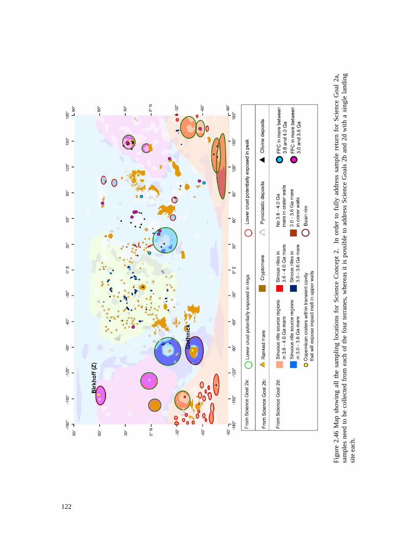
122
Fig
ure
2.4
6 M
ap s
ho
win
g a
ll t
he
sam
pli
ng
lo
cati
on
s fo
r S
cien
ce C
on
cep
t 2
. I
n o
rder
to
fu
lly
add
ress
sam
ple
ret
urn
fo
r S
cien
ce G
oal
2a,
sam
ple
s n
eed
to
be
coll
ecte
d f
rom
eac
h o
f th
e fo
ur
terr
anes
, w
her
eas
it i
s p
oss
ible
to
ad
dre
ss S
cien
ce G
oal
s 2
b a
nd
2d w
ith
a s
ing
le l
and
ing
site
eac
h.

123
SCIENCE CONCEPT 2 FINAL MAPS
The geophysical and sample return elements of Science Concept 2 are shown together in Fig. 2.47 and
2.48. Figure 2.47 shows all the possible tetrahedral configurations for the geophysical packages along with
the sample return elements. This map shows that it is possible to sample for at least one of the Science
Goals at one or two of the apices of the tetrahedral configuration, but it is not possible to complete all
aspects of the sample return within this Science Concept using a tetrahedral configuration. It is therefore
suggested that the sample return and geophysical elements of Science Concept 2 be kept separate, but that a
geophysical package is included at all sampling sites. This will ensure that neither the geophysical nor the
sample return elements of this Science Concept will be compromised. The addition of further geophysical
packages at sampling sites can then be used to add complexity to the baseline understanding obtained using
the geophysical configuration alone, by providing additional data at sites that have properties outside of
what is thought to be typical for that terrane, such as anomalously thick or thin crust. These data can be
used to provide better constraints on models of crustal thickness, the thermal state of the Moon, and mantle
density and composition.
Figure 2.48 shows all the tetrahedral configurations that satisfy the entirety of Science Goal 2d, and the
sample return elements of Science Goals 2a and 2b. This demonstrates that some of the configurations
shown in Fig. 2.48 for Science Goal 2d overlap with sampling sites for Science Goal 2b and part of Science
Goal 2a. Because there is not an ‗ideal‘ configuration of four landers which enables all the geophysical and
sampling elements of the whole Science Concept to be completed, additional landings are required to
address Science Concept 2as a whole.
A maximum of eight landers is required to fully address the geophysical and sample return aspects of
Science Concept 2. However there is likely to be overlap between at least one of the geophysical and
sample return sites, such that seven landing sites may be sufficient to address this Science Concept.
Assuming a geophysical package is added at each of the landing sites, a total of seven geophysical
packages would be placed on the surface for this proposal. The nature of the sampling studies means that
some of these sites are likely to be at locations of relatively thin crust, as many of the sampling sites are
within basins or large complex craters, and thus will improve the models as discussed above.
Though a strict tetrahedral configuration of four landing sites has been used above, it may be possible to
relax the tetrahedral configuration if more than four sites are chosen whilst maintaining global coverage of
a passive seismic network. This may enable better sampling sites to be chosen and fewer total landing sites
to be required; however, it would still not be possible to sample all lunar materials required to address this
Science Concept.

124
Fig
ure
2.4
7 F
inal
map
dis
pla
yin
g b
oth
geo
phy
sica
l an
d s
amp
le r
etu
rn a
spec
ts f
or
all
Sci
ence
Go
als
in S
cien
ce C
on
cep
t 2
, w
ith
th
e te
trah
edra
l
geo
phy
sica
l co
nfi
gu
rati
on
s sa
tisf
yin
g o
nly
th
e g
eop
hy
sica
l re
qu
irem
ents
for
the
Sci
ence
Con
cep
t.

125
Fig
ure
2.4
8 F
inal
map
dis
pla
yin
g b
oth
geo
ph
ysi
cal
and
sam
ple
ret
urn
asp
ects
fo
r al
l S
cien
ce G
oal
s in
Sci
ence
Co
nce
pt
2.
Her
e, t
he
tetr
ahed
ral
con
fig
ura
tio
ns
sati
sfy
Sci
ence
Go
al 2
d o
nly
, sh
ow
ing
th
at t
her
e ar
e si
tes
that
par
tial
ly o
ver
lap
wit
h S
cien
ce
Go
als
2a
and 2
b.

126
GEOPHYSICAL CASE STUDY: A33 MOONQUAKE NEST
The A33 moonquake is used here as a case study example to address the geophysical aspects of Science
Concept 2 (Fig. 2.49 to 2.52). This case study therefore uses the A33 moonquake nest to study the size and
state of the core, as in Science Goal 2c, combined with a tetrahedral seismic configuration required for
global mantle structure. One station needs to be placed within each of the areas within the white
boundaries shown in Figs. 2.49 and 2.50, with the latter figure also excluding areas not appropriate for heat
flow measurements. The configurations shown in Fig. 2.51 indicate the possible nearside locations of the
geophysical package as part of a strict tetrahedral configuration, and Fig. 2.52 shows a global view of these
locations (i.e., including farside stations). This configuration allows for two LLR stations to be placed on
the nearside, which will increase the extent of the current LLR network. As before, it would be preferable
to place an additional geophysics lander with an LLR station in the southern hemisphere to improve the N-
S extent of the current LLR network. It would also be ideal to place clusters of three geophysics packages
at each apex of the tetrahedron configuration, to begin to address shallow moonquake distribution and
upper mantle structure (but only within these clusters).
FIGURE 2.49 Map showing the same data as Fig. 2.30, but applied only to areas within S1 of the A33
antipode (left), and within 60° of the A33 nest (right). This would be applicable if seismology and
retroreflectors were to be combined in the same package and used A33 as the moonquake nest to study the
lunar core.
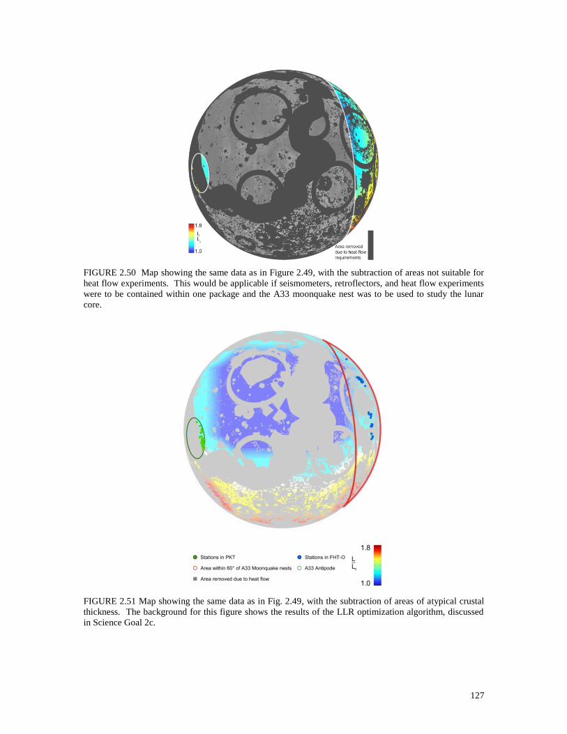
127
FIGURE 2.50 Map showing the same data as in Figure 2.49, with the subtraction of areas not suitable for
heat flow experiments. This would be applicable if seismometers, retroflectors, and heat flow experiments
were to be contained within one package and the A33 moonquake nest was to be used to study the lunar
core.
FIGURE 2.51 Map showing the same data as in Fig. 2.49, with the subtraction of areas of atypical crustal
thickness. The background for this figure shows the results of the LLR optimization algorithm, discussed
in Science Goal 2c.
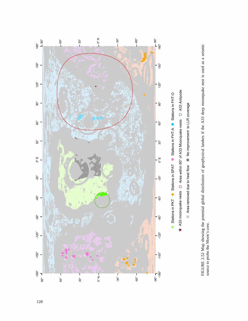
128
FIG
UR
E 2
.52
Map
sh
ow
ing
th
e p
ote
nti
al g
lob
al d
istr
ibu
tio
n o
f g
eop
hy
sica
l la
nd
ers
if t
he
A3
3 d
eep
mo
onq
uak
e n
est
is u
sed
as
a se
ism
ic
sou
rce
to p
rob
e th
e M
oon
‘s c
ore
.

129
SAMPLE RETURN CASE STUDY 1: MOSCOVIENSE
Moscoviense is located on the lunar farside (FHT-A terrane) at ~26˚N, 148˚E and is Nectarian in age
(Wilhelms et al., 1987). This basin was chosen as a case study as it hosts a range of mantle derived
materials (pyroclastic deposits, mare basalts, cryptomaria), and preserves a peak ring which may have
originated from depths within the mantle and most probably samples both upper and lower crust.
Example landing sites have been selected within Moscoviense basin: from north to south, these are
identified as sites 1, 2 and 3.
Site 1 is located in the topographic low of the basin, proximal to outcrops of the peak ring.
Within the 10 km buffer, low-Ti basalt could be sampled, as well outcrop and rubble of the
peak ring. From SELENE-SP detections the peak ring outcropping here may be of mantle
material (Yamamoto et al., 2010). At the 30 km buffer this site intersects olivine as
detected by Pieters et al. (2011). The 20 and 30 km buffer also overlap with the unit Im
(Kramer et al., 2008) which may represent impact melt from basin formation (Thaisen et
al., 2011).
Site 2 is located on the basin floor at the junction between the southern pyroclastic deposit
as mapped by Craddock et al. (1997) and the Im unit and the 10, 20 and 30 km buffer
zones intersect with the unit Iltm (Kramer et al., 2008). This site is proximal to the peak
ring of the basin, and although not close to detections of olivine by Kayuga it is close to
detections of low-Ca pyroxene and spinel (Pieters et al., 2011).
Site 3 is located in a topographic low in the area between the peak ring and the inner ring
(Figure 2.53). It is located within the cryptomare unit as identified by Hawke et al.
(2005a), and is proximal to three detections of olivine (Yamamoto et al., 2010). From this
site it is expected that outcrop and rubble of both the peak ring and inner peak could be
sampled.
SAMPLE RETURN CASE STUDY 2: NECTARIS
Nectaris is located on the lunar nearside, at the southeastern edge of the Procellarum KREEP Terrane
(~16oS, 35
oE) and is Nectarian in age. This basin contains at least two mare units, multiple pyroclastic
deposits, two floor-fractured craters, and spectrally-detected olivine (Coombs et al., 1990; Gaddis et al.,
2003; Hawke et al., 1997; Kramer et al., 2008; Schultz et al., 1976; Yamamoto et al., 2010), in addition to
peak rings (Whitford-Stark, 1981) that may preserve uplifted mantle or lower-crustal material (this study).
Three potential landing sites within the Nectaris basin have been identified:
Site 1 is the westernmost potential landing site, just south of the innermost peak-ring.
Samples of both a low-Ti mare basalt (Kramer et al., 2008) and peak ring material
(Whitford-Stark, 1981) could be sampled within the 10 km buffer. Pyroclastic glasses
originating near the Daguerre crater (Coombs et al., 1990; Hawke et al., 1997) could
potentially be sampled within this minimal buffer, but more likely within the 20 or 30 km
buffers around the proposed landing site.
Site 2 is the easternmost potential landing site and is located in a geologically-similar area
to Site 1. The same type of units could be sampled as in Site 1, though two different
pyroclastic glass units (Gaudibert and Gaudibert B; Cooms et al., 1990; Hawke et al.,
1997) may be encountered within the 30 km buffer as opposed to just one.
Site 3 is located nearer to the center of Nectaris basin and is the southernmost proposed
landing site. Within a 10-km buffer, two mare units (one low-Ti and one intermediate-Ti),
two pyroclastic units, and potentially two Copernican ejecta units can be sampled.

130
FIGURE 2.53 A) LOLA topographic DEM of Moscoviense and the corresponding topographic profile,
highlighting the stark difference between the uplifted basin rings and topographic lows. B) Approximate
location of the Moscoviense peak, inner and outer rings (as defined by Thaisen et al., 2011). This image
also identifies geomorphologic structures on the basin floor. C) Mapped geologic units within
Moscoviense basin. The pyroclastic deposit was mapped by Craddock et al. (1997); the cryptomare by
Hawke et al. (2005a). Spectrally determined mare units have been mapped by Kramer et al. (2008)
(denoted ˚ in key) where Ikm is a low-Ti unit, Iltm is a low-Ti unit, Im is a very low-Ti unit, and Intm is a
high-Ti unit. Spectral identifications have also been made by Pieters et al. (2011) (denoted * in the key)
and Yamamoto et al. (2010) (denoted x in the key). Floor-fractured craters are taken from Concept 5.
Three example landing sites are shown (1, 2, and 3 from N to S), with 10, 20 and 30 km buffer zones
around each. Note that the ranked mare intersection is from this study (see Science Goal 2b) and that the
point has a 30 km error associated with it.

131
FIGURE 2.54 A) LOLA topographic DEM of Nectaris and the corresponding topographic profile, showing
well-defined peak rings in the southwest compared to more muted topography in the northeast. B)
Approximate location of the Nectaris basin rings showing locations where they are certain, reasonably-
certain, and uncertain (Whitford-Stark, 1981). C) Mapped geologic units within Nectaris basin. The
pyroclastic deposits were mapped by Coombs et al. (1990), Hawke et al. (1997), and Gaddis et al. (2003),
and have been shown as blue circles correlating to their proposed areal extent (but note that this may not be
their actual distribution). Spectrally-determined units have been mapped by Kramer et al. (2008) where
Imtm is an Imbrian-aged, intermediate-Ti and Fe mare basalt, Iltm is an Imbrian-aged, low-Ti and low-Fe
mare (possibly high-Al), and Ec, Cc1, and Cc2 are Eratosthenian- and Copernican-aged crater ejecta,
respectively. Spectral identifications of olivine have also been made by Yamamoto et al. (2010). Two
floor-fractured craters (see Science Concept 5 and Schultz, 1976) are shown in the outer rings of Nectaris
and are identified by red circles. Three example landing sites are shown with 10, 20, and 30 km buffer
zones around each.

132
Top Related