


Languages
Pages
Legal


SAD Investors:
Implications of Seasonal Variations in Risk Aversion
by
Mark J. Kamstra, Lisa A. Kramer, and Maurice D. Levi∗
August 2003
JEL Classification: G1Keywords: seasonal risk aversion; bond return seasonality;
CRSP deciles; mutual fund flows
∗ Kamstra (Corresponding Author): Atlanta Federal Reserve Bank, 1000 Peachtree Street NE, Atlanta GA30309; Tel: 404-498-7094; Email: [email protected]. Kramer: Rotman School of Management,University of Toronto, 105 St. George St., Toronto Ont., M5S 3E6, Canada. Tel: 416-921-4285; Fax: 416-971-3048; Email: [email protected]. Levi: Faculty of Commerce and Business Administration,University of British Columbia, 2053 Main Mall, Vancouver BC, V6T 1Z2, Canada. Tel: 604-822-8260; Fax:604-822-4695; Email: [email protected]. We have benefited from valuable conversations withRamon DeGennaro, Mark Fisher, Michael Fleming, Scott Frame, Ken Garbade, Rob Heinkel, Alan Kraus,Paula Tkac, and seminar participants at the Federal Reserve Bank of Atlanta and the University of BritishColumbia. We gratefully acknowledge financial support of the Social Sciences and Humanities ResearchCouncil of Canada. Any remaining errors are solely the responsibility of the authors. The views expressedhere are those of the authors and not necessarily those of the Federal Reserve Bank of Atlanta or the FederalReserve System.
SAD Investors:
Implications of Seasonal Variations in Risk Aversion
Abstract
Previous research has shown that stock market returns appear to be associated with
variations in the incidence of seasonal affective disorder, SAD, during the fall and winter. The
medical and psychology literatures have clinically established a positive relationship between
the length of night and depression through the seasons, as well as a positive relationship
between depression and risk aversion. A seasonal pattern exists in stock returns, consistent
with SAD-influenced individuals buying and selling risky assets in response to changes in
their levels of risk aversion caused by seasonal depression. The present paper considers
whether SAD is associated with seasonalities in other financial markets, specifically returns
on government bonds, returns on stock portfolios of different risk classes, and flows of capital
into and out of mutual funds of different risk. We show statistically and economically
significant evidence from considering these other measures, consistent with a widespread,
SAD-influenced seasonal movement of investment funds into and out of various investment
vehicles.

In a recent paper, Kamstra, Kramer, and Levi (2003, henceforth KKL) show that there
is an economically and statistically significant seasonal regularity in stock market returns
that is consistent with the influence of seasonal affective disorder (SAD) on investors during
the fall and winter. Specifically, KKL argue that stock returns are influenced when many
people are suffering from depression due to SAD, or the milder “winter blues,” as a result
of increased length of night (or equivalently, reduced length of day) in the fall and winter.
Clinical and experimental studies in the medical, psychology, and economics literatures in-
dicate that seasonal reduction in hours of daylight leads to depression for many people, and
further studies show depression leads to heightened risk aversion. KKL hypothesize that
increased risk aversion among SAD-affected investors in the fall causes those investors to
sell risky stock, and then investors resume risky holdings with the reduction in risk aversion
that comes with increasingly abundant daylight in the new year. KKL find a striking annual
cycle in international stock market returns consistent with their hypothesis, even after con-
trolling for established market seasonalities such as tax-loss selling and potentially relevant
environmental factors such as temperature and cloud cover. Stock market returns are lowest
on average during the fall months when the number of hours of daylight is falling toward its
annual minimum. Mean stock returns are then highest as daylight becomes more plentiful in
the new year. In addition, the annual stock market return cycle due to SAD has greater am-
plitude at higher latitudes where the variations in length of night across seasons are greatest.
Furthermore, the patterns in stock returns in Northern versus Southern Hemisphere markets
are six months out of phase, as are the seasons.
If the SAD / depression / risk aversion hypothesis is correct, seasonal patterns should
exist in other markets. For instance, the returns on relatively safe government bond indices
should display a reverse seasonal relative to stock returns; the seasonal pattern in stock
returns should be more pronounced in risker classes of stocks; and there should be evidence
of a seasonal pattern in the flow of funds between risky and safe assets.
The underlying returns model in which seasonality in equity and bond returns are the
1

mirror image of each other may be considered in the following way. Suppose there are two
groups of investors, those who suffer from SAD and those who do not. Each group holds
a portfolio containing equities and bonds. In the fall, SAD sufferers become depressed and
consequently more risk averse, and they wish to hold relatively fewer equities and relatively
more bonds. The preferences of the non-sufferers do not change with the season. Since
all equities and bonds must ultimately be held, the non-sufferers must be persuaded to
buy the equities that the SAD sufferers wish to sell, and to sell some of their bonds, the
preference for which has not changed among the non-sufferers. Equity prices are depressed
in the fall as a consequence of the reduced demand for equities by the SAD-sufferers, thereby
raising expected equity returns. At the same time, increased demand for bonds by the SAD
sufferers raises their prices in the fall, hence lowering their expected returns and increasing
the willingness of the non-sufferers to sell their bonds to the other group. Equilibrium
is restored with equities flowing from SAD to non-SAD investors and bonds flowing from
non-SAD to SAD investors. The opposite happens in the spring as the days lengthen.
We aim to determine whether there are seasonal regularities in other parts of the capital
market that are consistent with this model. Specifically, we seek answers to the following
questions:
1. When people are experiencing changes in risk aversion as a consequence of SAD, ini-
tially selling stocks (leading to stock prices which rise less quickly in the fall than they
would otherwise) and later repurchasing stocks (leading to higher prices and therefore
higher returns in the winter), are stock sellers (buyers) simultaneously buying (selling)
low or zero default-risk Treasury bonds, influencing the price of bonds and affecting
their returns? That is, is the seasonal pattern of risk-free bond returns the reverse
of the seasonal pattern of stock returns: low bond returns when stock returns due to
SAD are highest, and vice versa?
2. When SAD sufferers are shunning risk, does this result in less willingness to hold the
riskier end of the stock market spectrum than the safer end? In other words, does the
2

seasonal pattern of stock returns of different deciles of risk – measured by, for example,
company beta (systematic risk) or standard deviation of returns (total risk) – match
what we would expect from SAD, namely a larger amplitude of seasonal variation
for the riskier companies and relatively muted seasonal variation for the less risky
companies? A risk-related seasonal pattern in stock returns is suggested but not fully
explored by KKL: they find SAD has a more pronounced effect on an equally-weighted
aggregate stock market index than on a value-weighted index, with equal weighting
placing greater relative importance on smaller (riskier) companies.
3. Do flows into and out of mutual funds reflect patterns that are consistent with the
SAD hypothesis, with capital flowing out of risky stock funds and into safe bond funds
during times when increased length of night leads to higher levels of risk aversion
among affected individuals? Does capital flow out of bond funds and back into stock
funds when daylight becomes more abundant?
Evidence from answering these questions would help clarify the importance of seasonal af-
fective disorder for asset return regularities in financial markets.
The remainder of the paper is organized as follows. In Section 1, we discuss the medical
condition of SAD and explain how SAD can translate into an economically significant influ-
ence on capital markets. In Section 2, we define the measure we use to capture the impact
of SAD on financial markets. We present evidence in Section 3 that seasonal depression has
an impact on bond market returns that is consistent with (and opposite to) the pattern that
has been shown to exist in markets for risky stock. In Section 4 we consider risk-sorted stock
deciles and determine that the magnitude of the SAD effect on returns varies directly with
riskiness of the stock portfolio. In Section 5 we present evidence that the flow of capital into
and out of mutual funds follows a seasonal pattern consistent with SAD. Section 6 concludes.
3
1 Seasonal Affective Disorder and Risk Aversion
There are two essential components to a link between seasonalities in length of night and
different manifestations of risk aversion:
1. That seasonal variations in length of night result in seasonal variations in the incidence
of depression and the less serious condition “winter blues.”
2. That variations in depression or winter blues are associated with variations in risk
aversion; specifically, that risk aversion rises with depression.
Both of the above connections are well supported and extensively documented in clinical
psychology and medical studies that consider both behavioral and biochemical evidence.
As for the impact of seasonal cycles in daylight on SAD, the evidence fills many books and
research journals, where some of the journals are devoted to papers on affective (emotional)
disorders, particularly of the seasonal variety. Indeed, there are numerous books telling
people how to deal with this disorder, and many products which create “natural” light to help
sufferers handle their condition. Examples of recent popular books devoted to considering
seasonal affective disorder and therapies for dealing with it are Rosenthal (1998) and Lam
(1998). Among the literally hundreds and perhaps thousands of journal articles on the
pervasiveness and potential severity of SAD are papers by Cohen et. al. (1992), Faedda et.
al. (1993), Molin et. al. (1996), and Young et. al. (1997). The large and growing volume of
books, articles, and products dealing with seasonal affective disorder is testimony to the fact
that this condition is a very real and extensive problem, estimated to influence at least 10
million Americans severely, 15 million Americans mildly, and many more millions in other
countries ranging from those near polar extremes to those as close to the equator as India.
Symptoms of SAD include anxiety, prolonged periods of sadness, chronic fatigue, difficulty
concentrating, reduced energy, lethargy, sleep disturbance, sugar and carbohydrate craving
with accompanying weight gain, loss of interest in sex, and of course clinical depression.1
1For extensive references to the literatures covering these matters see Kamstra, Kramer, Levi (2003).
4

There is also a large and growing literature on the second link mentioned above, namely,
between depression and risk taking behavior. This link has been documented in both fi-
nancial and non-financial settings. The aspect of risk that is most commonly studied in the
psychology literature is the tendency for depressed people to avoid being “sensation seekers.”
In principle, depressed people could throw caution to the wind, or they could become conser-
vative in their behavior. The evidence strongly supports the latter: depression is associated
with reduced sensation seeking tendencies which in financial settings translates to increased
risk aversion. For example, Carton et. al. (1992) test whether depressive mood reduces
sensation seeking and conclude that it does. Horvath and Zuckerman (1993) consider both
the connection between depression and sensation seeking and how depressed people evalu-
ate risk. Two other papers by Zuckerman (1980, 1984) show how depression emerges as a
correlate with reduced sensation seeking when considered in the context of other potential
biological factors. Eisenberg, Baron, and Seligman (1998) consider individuals’ risk aversion
and the role of anxiety in the willingness to take chances.
Examples of papers that explore the extension from sensation seeking into the financial
context include Harlow and Brown (1990) and Wong and Carducci (1991). Wong and Car-
ducci find that individuals who score low on tests of sensation seeking display greater risk
aversion in making financial decisions, including the decision to purchase stocks, bonds, and
automobile insurance. Harlow and Brown shed light on the link between sensation seeking
and financial risk inclination by building on results from psychiatry which show that high
blood levels of the enzyme monoamine oxidase are associated with depression and a lack of
sensation seeking while low levels of monoamine oxidase are associated with a high degree of
sensation seeking.2 Harlow and Brown had 183 test subjects participate in sequences of first
price sealed bid auctions. They determined the quantitative sensation seeking score for each
subject and also measured participants’ blood levels of various neuroregulating enzymes.
Summarizing the results of their parametric and non-parametric analyses, they state “Indi-
2See Zuckerman (1983), Hirschfeld (2000), and Delgado (2000) for further discussion of the biochemistryof depression and sensation seeking.
5

viduals with neurochemical activity characterized by lower levels of the enzyme monoamine
oxidase and with a higher degree of sensation-seeking are more willing to accept economic
risk ... Conversely, high levels of this enzyme and a low level of sensation seeking appear to
be associated with risk-averse behaviour.” (pages 50-51, emphasis added). These findings
are consistent with an individual’s level of sensation seeking being indicative of his or her
degree of financial risk aversion, an important link in the mechanism that ties the depression
associated with seasonal affective disorder to widespread effects in financial markets.
2 Measuring the Impact of SAD
In order to evaluate the manifestation of seasonal variations in daily light and darkness on
financial markets, we must first decide how to measure the causal variable.3 We choose to
use the length of the night at New York’s latitude, 41 degrees north. As KKL report, one
could similarly use the latitude from a different location in the continental US. The fact
that many market participants initiate trades from latitudes other than that of New York
does not adversely affect the mechanism underlying the SAD hypothesis, as length of night
follows a similar seasonal throughout a hemisphere, varying only in amplitude.
In this paper we focus on US evidence since we are investigating a range of market returns
and mutual fund flows that are more readily available for the United States. To obtain the
daily number of hours of night in New York, we first need to calculate the sun’s declination
angle, λt:
λt = 0.4102 · sin[(
2π
365)(juliant − 80.25)
], (1)
where julian varies from 1 to 365 (366 in a leap year), taking the value 1 for January 1, 2 for
January 2, and so on. We can then calculate the number of hours of night, Ht, at latitude
3Note that KKL (2003) find empirical evidence that the driving force behind the SAD effect they documentis length of night (the time between sunset and sunrise), not sunshine (which varies according to percentagecloud cover). They find that additionally controlling for sunshine does not materially change the sign orsignificance of SAD-related variables or any other variables in their regressions. Further, the sunshine variableis typically statistically insignificant across the nine countries they consider.
6

δ (41 degrees):
Ht =
24 − 7.72 · arccos[−tan(2πδ
360)tan(λt)
]in the Northern Hemisphere
7.72 · arccos[−tan(2πδ
360)tan(λt)
]in the Southern Hemisphere,
(2)
where arccos is the arc cosine. Note that when working with monthly, as opposed to daily
data, we define Ht as the median monthly hours of night.
Medical practitioners have determined that depression and other symptoms associated
with the most common form of SAD are isolated to the fall and winter. Symptoms of
fall/winter SAD (commonly known as winter SAD) can start as early as autumn equinox
and may persist as late as spring equinox, as discussed by Dilsaver (1990) and others. A
rarer condition called summer SAD or reverse SAD affects about a fifth as many people as
winter SAD, and it can cause symptoms that start in the spring and last as late as the end
of summer. While the cause and effect of winter SAD are well documented, psychologists’
understanding of summer SAD is still preliminary, with high temperature, not changes in
the amount of daylight, thought to be the most likely trigger. In this paper, we investigate
the financial implications of winter SAD only.
We define our SAD measure as follows, taking on non-zero values only during the seasons
when the length of day is well understood to have an influence on individuals’ behavior:
SADt =
{Ht − 12 for trading days in the fall and winter0 otherwise.
(3)
By deducting 12 from the number of hours of night (Ht), SADt measures the length of the
night in winter and fall relative to the mean annual number of hours of night. (We define the
SAD measure in terms of number of hours of night, the time from sunset to sunrise, though
in principle one could instead define the measure in terms of number of hours of daylight.)
As defined, the SAD measure equals zero at fall equinox and spring equinox, and takes
on positive values throughout the fall and winter months in between those two dates. Fur-
thermore, the value of the SAD measure is roughly the same during days in December as it
7

is during days in January, the SAD variable takes on about the same values during days in
November as it does on February days, and it is again about equal in value during the days
in October as it is during the days of March. As we describe below, however, we expect the
impact of seasonal depression on a given asset’s returns to take on different values in the
fall months versus the winter months. With equities, for instance, we expect SAD affected
investors to sell riskier assets in the fall and then buy them back after winter solstice as their
levels of risk aversion return to normal. As a consequence, equity prices should be lower
in the fall than they would be without the elevated risk aversion amongst SAD affected
investors. That is, with rising risk aversion in fall, we expect stock prices to rise less quickly
relative to the rest of the year. Then, as daylight becomes more plentiful and risk aversion
declines, SAD-influenced investors start resuming their holdings of risky assets, with the
recovery of prices raising returns. Hence, we would expect lower stock returns in fall and
higher stock returns in winter than would be expected in the absence of a SAD effect.
The SAD variable is itself incapable of capturing a pattern where opposing effects are
expected across the fall and winter months, hence we additionally use a dummy variable for
the fall:4
DFallt =
{1 for trading days in the fall0 otherwise.
(4)
Inclusion of this dummy variable allows but does not require the impact of SAD to differ
across the fall and winter seasons. The relevance of the difference in the magnitude of the
SAD effect across the fall and winter can be judged by the magnitude and significance of
this fall dummy variable. The total impact of seasonal depression on returns is measured
collectively by the SAD variable and the fall dummy variable. This parameterization with
two variables permits the impact of seasonal depression on returns in the fall months to differ
from that in the winter months, as we expect.
4We define the fall as September 21 through December 20 in the context of daily data, and Octoberthrough December when working with monthly data.
8
3 The Bond Market
When investors become less willing to bear risk and perhaps liquidate portions of their stock
portfolios, the implication is that the funds raised ought to be placed in relatively safer assets
such as government bonds. Hence, when stock prices are declining (or rising less quickly)
as a result of the trading activity of depressed individuals, bond prices may be rising. This
suggests the seasonal stock and bond market patterns should be the reverse of one another
during the fall and winter seasons when length of night influences investor sentiment.5
To investigate whether there are reverse seasonal patterns in the stock and bond markets
related to SAD, we consider returns to holding US Treasury bonds. We choose US govern-
ment bonds because they represent the least risky of fixed income securities and hence are
likely to be seen by investors as the favored alternative to risky equities. We select return
indices for various Treasury bond maturities ranging from 1 year to 10 years, where the
returns include interest and capital gains/losses. These data are obtained from the Center
for Research on Security Prices (CRSP) US Treasury and Inflation Series. The series contain
returns from the CRSP US Treasury Fixed Term Index Series and the CRSP Risk Free Rates
File. The frequency of the returns is monthly.
In Table 1, we present summary statistics on the monthly Treasury bond index returns.
Each series begins in January, April, or May 1941, as available through CRSP. The series all
end in December 2001. The mean monthly returns and return standard deviations typically
increase with maturity. Average returns from holding the various government bond series
are slightly below one-half percent per month. That is, average annual returns on risk-free
US Treasury bonds over the last 60 years are approximately five percent. Returns vary
substantially from month-to-month on all maturity bonds, especially for the longer maturity
bonds, with some months’ losses being around seven percent and some months’ returns well
5While some market circumstances, such as bad news about the economy, can cause the bond and stockmarkets to move in opposite directions, there are other events, such as interest rate movements, that canmake them move in the same direction. Our emphasis here is on seasonal regularities in bond and stockmarkets, unrelated to exogenous macroeconomic shocks.
9

over ten percent. Of course, these large gains and losses are due to variations in the bond
prices. As in the stock market, returns are skewed to the right and leptokurtotic.
Since we hypothesize that the SAD seasonal in bond returns will be opposite in sign
relative to stock returns, it is helpful to consider first whether our monthly bond index
returns are unconditionally correlated with stock returns. If stock and bond returns are
highly negatively correlated, then it may not be surprising to find bond returns display an
opposite SAD seasonal relative to stock returns. If, however, there is positive correlation
between stock and bond returns, then finding opposite SAD seasonals in bond returns relative
to stock returns would be all the more remarkable. Table 2 contains correlation coefficients
based on the covariance between the each of the monthly government bond index returns
and monthly CRSP total stock market index returns for various sample periods. Note that
for the full sample period, the bond returns are significantly positively correlated with stock
returns. In each of the decade sub-periods, stock and bond returns are either significantly
positively correlated or insignificantly negatively correlated, with the single exception of the
5 year bond index in the 1950s. Thus we can safely assert that the tests we present below
for an opposite SAD seasonal in bonds relative to stocks are not unduly biased in favor of
the result we expect.
In Figure 1 we plot the average monthly percentage returns on the bonds we consider,
expressed on an annualized basis. Omitted plots based on individual monthly bond returns,
as opposed to the average returns across the series, are very similar. Note the returns we
plot are unconditional; conditional analysis is presented later. Returns are very high in
the fall months, September, October, and November. Returns drop through the winter,
reaching a low in February. The difference in the average returns from October to February
is particularly striking: about 7 percent on an annualized basis. The overall pattern is
consistent with investors moving funds into safe government bonds in the fall, driving up
prices and hence returns, and then moving funds out of government bonds with the increase
10
in daylight that commences with winter, lowering returns.6
To more fully evaluate the quantitative impact of SAD on bond returns, we estimate a
set of regressions for the bond return indices, allowing the magnitude of the SAD coefficient
to differ across indices. Based on the seasonal cycle of SAD, we expect to find patterns that
are opposite to those found by KKL for stock market returns: when SAD-induced changes
in risk aversion cause stock returns to rise, bond returns should fall, and vice versa. We
estimate the following model, controlling for well-known market seasonals:7
ri,t = µ + ρi,1ri,t−1 + µi,SADSADt + µi,FallDFallt + µi,TaxD
Taxt + εi,t (5)
Variables are defined as follows: ri,t is the month t return for a given bond index (i indicates
the bond series, with 1, 2, 5, 7, or 10 year maturity), ri,t−1 is a lagged dependent variable,
SADt equals Ht − 12 during fall and winter months (October through March) and equals
zero otherwise (where Ht is the median monthly number of hours of night in period t), DFallt
is a dummy variable which equals one when month t is in the fall (October, November,
and December) and equals zero otherwise, and DTaxt equals one for the month of January
and equals zero otherwise. We report below results of testing the one-sided null hypotheses
that µSAD < 0 and µFall > 0, with the inequalities suggested by evidence from the medical,
psychology, and experimental economics literatures discussed in the previous sections. Note,
however, that throughout the paper we conservatively report significance based on two-sided
tests.
The five bond return series, for the 1, 2, 5, 7, and 10 year bonds, form a panel-time-
series data set. Estimating Equation 5 jointly across the indices using Hansen’s (1982)
6The relatively smoother behavior of returns during the spring and summer months, April through August,is beyond the scope of this study. We focus on the fall and winter (September through March), the seasonsduring which the effects of length of day on mood are well understood by medical professionals.
7Some of the papers that document seasonalities in returns of various classes and maturities of bondsinclude the following. Schneeweis and Woolridge (1979) document the presence of autocorrelation in bondindex returns. Schneeweis and Woolridge (1979), Chang and Huang (1990), and Wilson and Jones (1990)demonstrate the presence of a January seasonal in various US bond returns. While we don’t consider dailybond returns in this study, Jordan and Jordan (1991) find there is no evidence of a day-of-the-week effect incorporate bonds over the past few decades.
11
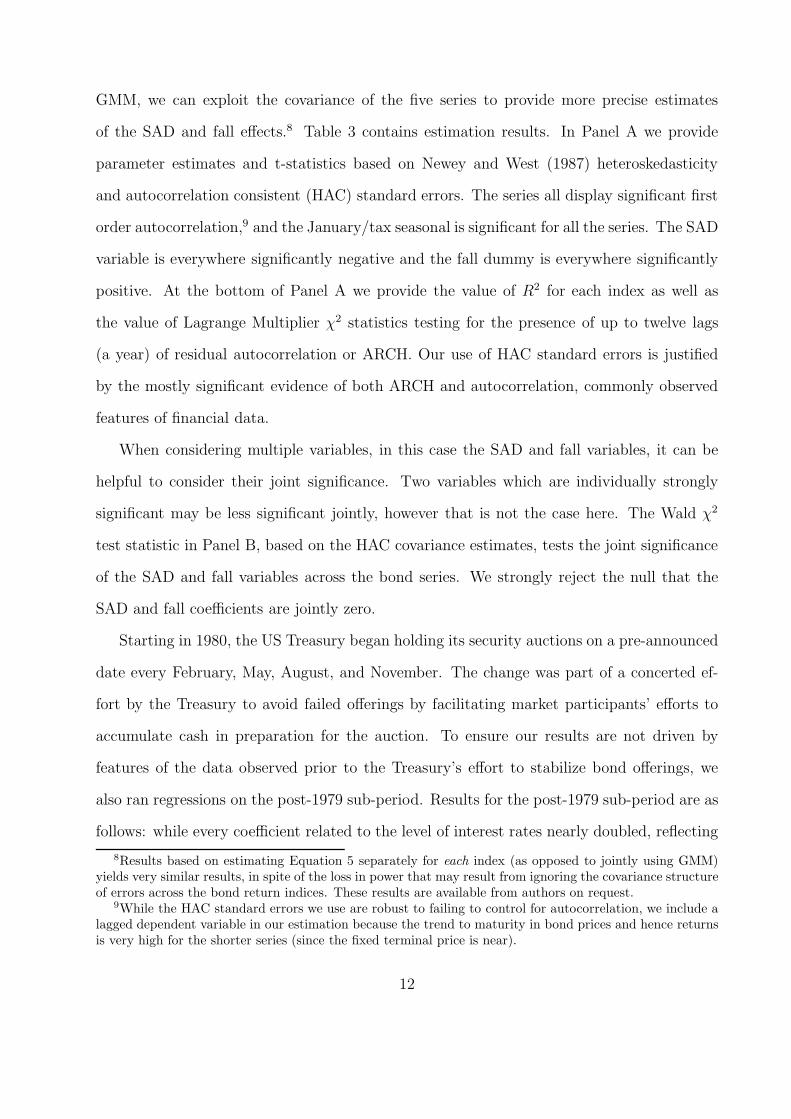
GMM, we can exploit the covariance of the five series to provide more precise estimates
of the SAD and fall effects.8 Table 3 contains estimation results. In Panel A we provide
parameter estimates and t-statistics based on Newey and West (1987) heteroskedasticity
and autocorrelation consistent (HAC) standard errors. The series all display significant first
order autocorrelation,9 and the January/tax seasonal is significant for all the series. The SAD
variable is everywhere significantly negative and the fall dummy is everywhere significantly
positive. At the bottom of Panel A we provide the value of R2 for each index as well as
the value of Lagrange Multiplier χ2 statistics testing for the presence of up to twelve lags
(a year) of residual autocorrelation or ARCH. Our use of HAC standard errors is justified
by the mostly significant evidence of both ARCH and autocorrelation, commonly observed
features of financial data.
When considering multiple variables, in this case the SAD and fall variables, it can be
helpful to consider their joint significance. Two variables which are individually strongly
significant may be less significant jointly, however that is not the case here. The Wald χ2
test statistic in Panel B, based on the HAC covariance estimates, tests the joint significance
of the SAD and fall variables across the bond series. We strongly reject the null that the
SAD and fall coefficients are jointly zero.
Starting in 1980, the US Treasury began holding its security auctions on a pre-announced
date every February, May, August, and November. The change was part of a concerted ef-
fort by the Treasury to avoid failed offerings by facilitating market participants’ efforts to
accumulate cash in preparation for the auction. To ensure our results are not driven by
features of the data observed prior to the Treasury’s effort to stabilize bond offerings, we
also ran regressions on the post-1979 sub-period. Results for the post-1979 sub-period are as
follows: while every coefficient related to the level of interest rates nearly doubled, reflecting
8Results based on estimating Equation 5 separately for each index (as opposed to jointly using GMM)yields very similar results, in spite of the loss in power that may result from ignoring the covariance structureof errors across the bond return indices. These results are available from authors on request.
9While the HAC standard errors we use are robust to failing to control for autocorrelation, we include alagged dependent variable in our estimation because the trend to maturity in bond prices and hence returnsis very high for the shorter series (since the fixed terminal price is near).
12

the higher average interest rates post-1979, the signs, relative magnitudes and statistical sig-
nificance of all the model coefficient estimates including the SAD and fall variables remained
virtually unchanged with no qualitative differences compared to the results reported for the
full sample. These results are available from the authors.
To enable discussion of the magnitude of the parameter estimates on the SAD and fall
dummy variables that arise from estimating Equation 5, we present in Table 4 the translation
of the SAD and fall parameter estimates into average annualized percentage returns. The
first value we present for each bond index in Table 4 is the total average annualized return,
which is between five and six percent for all the series. In the next column we present the
portion of the average annualized return that is explained by the SAD measure. To compute
the return due to SAD for a given index, we first calculate the value of the SAD variable
for each month. We multiply each month’s value by the index’s SAD variable estimate
shown in Table 3. We then compound across months, annualizing the result. In the last
column, we present the average annualized return due to the fall dummy variable for each
index, calculated by taking the value of the fall dummy variable for each month (one during
months in the fall, zero otherwise) multiplying by the value of the fall dummy variable
estimate for a particular index (from Table 3), compounding across months, converting the
result into an annualized return.
For each value in Table 4, two and three asterisks denote significance at the 5 percent
and 1 percent levels respectively, based on two-sided tests. In the case of the unconditional
return column, significance is based on t-tests for a mean return different from zero. In the
case of the columns for the annualized returns due to the SAD and fall dummy variables,
significance is simply carried over from the t-tests on the parameter estimates shown in
Table 3.
In a similar analysis of annual stock market returns due to the SAD and fall variables,
KKL showed that the portion of returns due to SAD was significantly positive for most
indices (in some cases exceeding the unconditional annual return itself) and the portion
13
of annual returns due to the fall variable was significantly negative for most stock indices
considered. Those results are consistent with SAD-affected investors selling risky stock in the
fall as they become less tolerant of risk, then resuming risky holdings after winter solstice,
as they return to their non-SAD-affected level of risk tolerance.
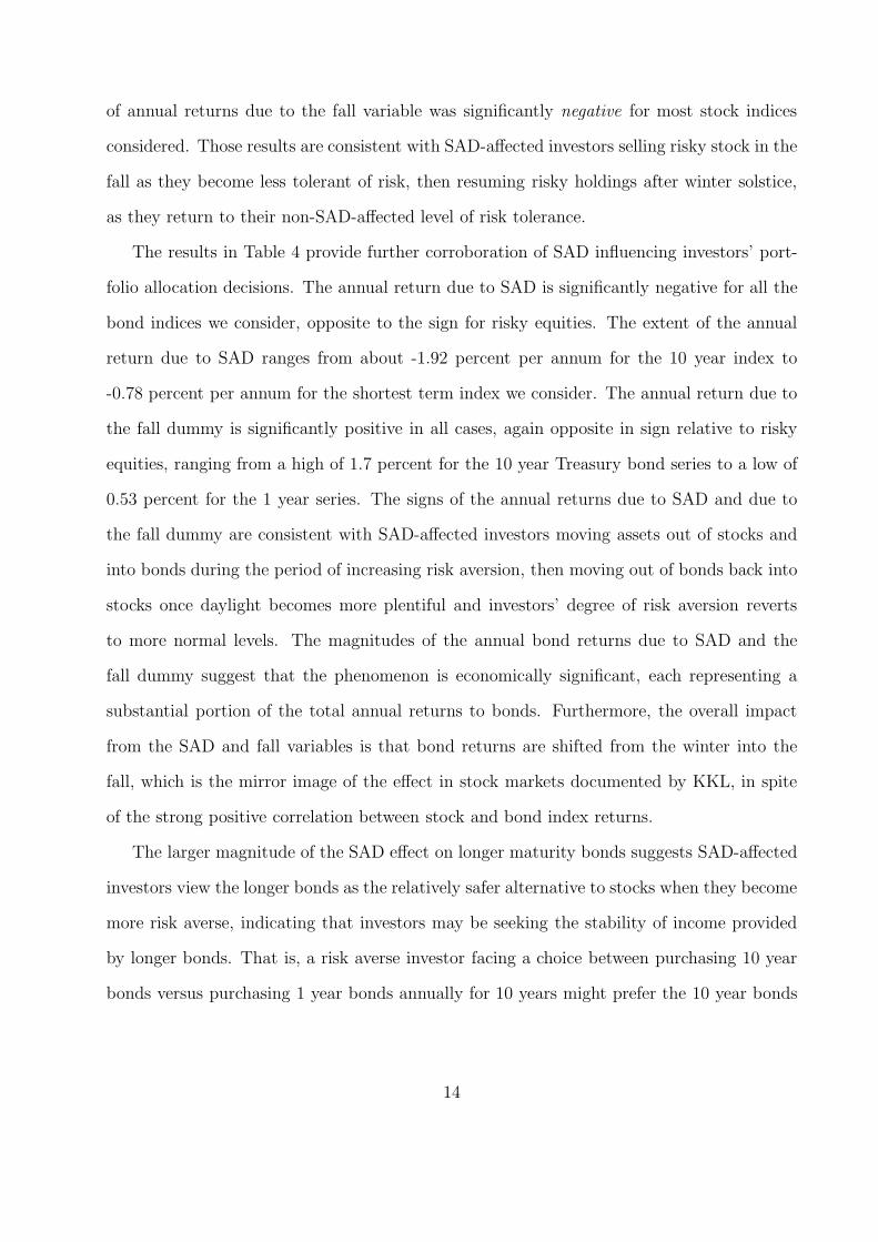
The results in Table 4 provide further corroboration of SAD influencing investors’ port-
folio allocation decisions. The annual return due to SAD is significantly negative for all the
bond indices we consider, opposite to the sign for risky equities. The extent of the annual
return due to SAD ranges from about -1.92 percent per annum for the 10 year index to
-0.78 percent per annum for the shortest term index we consider. The annual return due to
the fall dummy is significantly positive in all cases, again opposite in sign relative to risky
equities, ranging from a high of 1.7 percent for the 10 year Treasury bond series to a low of
0.53 percent for the 1 year series. The signs of the annual returns due to SAD and due to
the fall dummy are consistent with SAD-affected investors moving assets out of stocks and
into bonds during the period of increasing risk aversion, then moving out of bonds back into
stocks once daylight becomes more plentiful and investors’ degree of risk aversion reverts
to more normal levels. The magnitudes of the annual bond returns due to SAD and the
fall dummy suggest that the phenomenon is economically significant, each representing a
substantial portion of the total annual returns to bonds. Furthermore, the overall impact
from the SAD and fall variables is that bond returns are shifted from the winter into the
fall, which is the mirror image of the effect in stock markets documented by KKL, in spite
of the strong positive correlation between stock and bond index returns.
The larger magnitude of the SAD effect on longer maturity bonds suggests SAD-affected
investors view the longer bonds as the relatively safer alternative to stocks when they become
more risk averse, indicating that investors may be seeking the stability of income provided
by longer bonds. That is, a risk averse investor facing a choice between purchasing 10 year
bonds versus purchasing 1 year bonds annually for 10 years might prefer the 10 year bonds
14

to reduce the reinvestment uncertainty that arises every year for 1 year bonds.10
We conducted a variety of robustness checks. First, considering very short term (30-day
and 90-day) Treasury bills and very long term (20 year and 30 year) Treasury bonds leads
to results that are virtually indistinguishable from those presented above, with identical
signs and statistical significance for the SAD and fall variables. Second, results for daily
government bond indices (which are available to us only for relatively shorter time periods)
are also qualitatively identical to those we report above based on monthly data. Detailed
results are available from the authors on request.
4 Stock Portfolios of Differing Risk Class
If investors show changes in risk aversion associated with length of night, then this phe-
nomenon should reveal itself differently in stock portfolios with different amounts of risk.
Specifically, the riskier is the stock portfolio, the greater should be the size of the fluctuation
in returns due to SAD. Results reported in a supplemental appendix to KKL (2003)11 are
suggestive of differences in the SAD-related seasonality across portfolios of differing risk class:
SAD effects are more prominent in equal-weighted stock indices than in value-weighted stock
indices, consistent with equal-weighted indices’ relatively disproportionate representation of
small, risky firms. In this paper we directly investigate whether the SAD seasonal is stronger
in riskier portfolios.
We consider two measures of portfolio risk for examining the connection between risk and
return suggested by SAD: the magnitude of the portfolio beta and the standard deviation of
returns. Papers that consider stock portfolios sorted by beta or return standard deviation
include Fama and French (1992), Kothari, Shanken and Sloan (1995), and many others.
One procedure to consider possible differences in the size of various seasonalities exhibited
by portfolios of different risk or overall return volatility is to consider the return on the
10See Telser (1967) for further details on the argument that individuals who prefer certainty of income,perhaps for retirement planning, would prefer longer-lived assets.
11The appendix is available on the Web at at www.markkamstra.com.
15

extremes of the categorization deciles/quintiles.12 For example, returns on the quintile of
largest firms minus returns on the quintile of smallest firms can be examined for seasonality,
an approach that has been applied specifically in the study of turn-of-year effects, as by
Reiganum (1983), Rogalski and Tinic (1984) and Thaler (1987). In this paper we report the
full spectrum of results based on estimating the SAD effect in all the CRSP return deciles
sorted according to firms’ beta or standard deviation of returns, which according to CRSP
are constructed with equal-weighted returns.
In Table 5 we present summary statistics on daily CRSP decile returns, sorted on the
basis of beta in Panel A and sorted by the standard deviation of returns in Panel B. The
daily data span July 3, 1962 through December 31, 2001. Decile 1 denotes the category
of firms with the highest beta or return standard deviation, and 10 denotes the smallest.
Interpreting the beta and standard deviation sorting criteria as proxies for risk, the first
decile can be considered the most risky and the tenth the least. For each decile we present
the mean daily return, standard deviation of returns, minimum, maximum, skewness and
kurtosis, based on all 9942 observations. The mean daily returns are all fairly close to a
tenth of a percent for the beta-sorted deciles, while they are much more dispersed for the
standard-deviation-sorted deciles, trending down from about a fifth of a percent to about
a twentieth as we move from the most to the least variable return deciles. The standard
deviations are in the vicinity of 1 percent. The largest negative daily returns are between
about -10 percent and -20 percent, and the largest positive daily returns range up to about
15 percent. The series display varying degrees of skewness and kurtosis with both moments
tending to rise in magnitude as we move toward the 10th decile of both the beta and standard
deviation sorted return deciles.
We plot the unconditional monthly returns for each set of stock deciles in Figures 2 and 3.
We focus our attention on the fall and winter, the periods during which the influence of length
of night on individuals’ moods is well understood by medical professionals. Consider first
12See, for instance, Keim (1983), Reiganum (1983), Roll (1983), and the comprehensive study of seasonalityin risk premia on a wide range of assets by Keim and Stambaugh (1986).
16

Figure 2, returns for the beta-sorted deciles. The stock decile return series all demonstrate
a low in September or October, coincident with the point at which mean government bond
returns peak in Figure 1. The stock decile returns then reach their peak in January, the
time of year when mean bond returns are very nearly at their minimum. Notice that the
magnitude of the stock decile returns is roughly proportional to the risk class, with higher
risk deciles generally having higher returns than lower risk deciles. (The sole exception is
decile 10, corresponding to the lowest beta firms.) Furthermore, the seasonality, low returns
in fall and high returns in winter, preserves this ordinal ranking.
While the beta-sorted deciles reflect systematic risk, we can also examine unconditional
returns for deciles sorted on the basis of total risk, proxied by standard deviation of returns,
as shown in Figure 3. The fall and winter seasonal patterns are very similar to those displayed
in Figure 2. The ordinal ranking of returns across standard-deviation-sorted deciles is even
cleaner than for beta-sorted deciles: now the pattern is strongly monotonic. Overall, returns
are low in the fall and high in the winter for all the deciles, consistent with SAD-influenced
investors moving in and out of risky assets in accordance with length-of-day related changes
in risk aversion. Of course, these figures represent unconditional results, heavily influenced
by some conditional events, such as tax-loss selling.
To further evaluate the prominence of the SAD effect across deciles of different levels of
risk, we jointly estimate a set of regressions again making use of Hansen’s (1982) GMM and
Newey and West (1987) HAC covariance estimates. We expect the magnitude of estimates
on the SAD and fall variables to be larger for riskier deciles, consistent with SAD-affected
investors’ changing tolerance for risk through the fall and winter. The model we estimate is:
ri,t = µ + ρi,1ri,t−1 + µi,SADSADt + µi,FallDFallt + µi,MonD
Mont + µi,TaxD
Taxt + εi,t (6)
where ri,t is the trading day t return for CRSP decile i = 1, · · · , 10. As before, SADt equals
Ht − 12 during fall and winter and equals zero otherwise (where Ht is the daily number of
17
hours of night), and DFallt is a dummy variable which equals one when day t is in the fall
and equals zero otherwise. DMont equals one for the first trading day following a weekend,
usually a Monday. DTaxt equals one for the last trading day in December and the first five
trading days in January.13 Results based on controlling for autocorrelation in returns using
lags of the dependent variable are very similar to results presented below, and are available
from the authors on request.
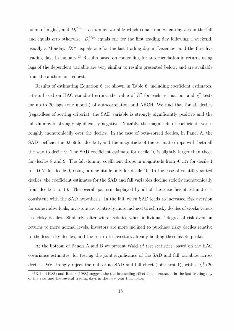
Results of estimating Equation 6 are shown in Table 6, including coefficient estimates,
t-tests based on HAC standard errors, the value of R2 for each estimation, and χ2 tests
for up to 20 lags (one month) of autocorrelation and ARCH. We find that for all deciles
(regardless of sorting criteria), the SAD variable is strongly significantly positive and the
fall dummy is strongly significantly negative. Notably, the magnitude of coefficients varies
roughly monotonically over the deciles. In the case of beta-sorted deciles, in Panel A, the
SAD coefficient is 0.066 for decile 1, and the magnitude of the estimate drops with beta all
the way to decile 9. The SAD coefficient estimate for decile 10 is slightly larger than those
for deciles 8 and 9. The fall dummy coefficient drops in magnitude from -0.117 for decile 1
to -0.051 for decile 9, rising in magnitude only for decile 10. In the case of volatility-sorted
deciles, the coefficient estimates for the SAD and fall variables decline strictly monotonically
from decile 1 to 10. The overall pattern displayed by all of these coefficient estimates is
consistent with the SAD hypothesis. In the fall, when SAD leads to increased risk aversion
for some individuals, investors are relatively more inclined to sell risky deciles of stocks versus
less risky deciles. Similarly, after winter solstice when individuals’ degree of risk aversion
returns to more normal levels, investors are more inclined to purchase risky deciles relative
to the less risky deciles, and the return to investors already holding these assets peaks.
At the bottom of Panels A and B we present Wald χ2 test statistics, based on the HAC
covariance estimates, for testing the joint significance of the SAD and fall variables across
deciles. We strongly reject the null of no SAD and fall effect (joint test 1), with a χ2 (20
13Keim (1983) and Ritter (1988) suggest the tax-loss selling effect is concentrated in the last trading dayof the year and the several trading days in the new year that follow.
18

degrees of freedom) test statistic of 57 in the case of beta-sorted deciles, and a χ2 (20 degrees
of freedom) statistic of 81.4 for the standard-deviation-sorted deciles. These results verify
that the individually significant SAD and fall coefficient estimates are also jointly significant.
The Wald test of the SAD coefficients being the same across deciles (joint test 2) strongly
reject this null in favor of the alternative of different coefficient values across deciles, for
both the beta- and standard-deviation-sorted deciles. Tests for the fall coefficient value to
be the same across deciles (joint test 3) are also strongly rejected for both the beta- and
standard-deviation-sorted decile returns. These last two tests indicate that the magnitude
of the SAD and fall variables vary significantly according to the risk of a portfolio.
In Table 7 we translate the SAD and fall dummy variable estimates from Table 6 into
more easily interpreted terms. Panel A pertains to the beta-sorted data and Panel B contains
results for standard-deviation-sorted deciles. For each decile, we present in the first column
the total average annualized return. In the next column, we present the average annualized
return that is explained by the SAD measure. To obtain this value, we multiply the value
of the SAD variable for each month, from Equation 3, by the SAD coefficient estimate from
Table 6. We then compound across periods and annualize the result. In the final column
of Table 7, we present the average annualized return due to the fall dummy variable for
each decile, computed similarly. For each value in Table 7, two and three asterisks denote
significance at the 5 percent and 1 percent levels respectively, based on two-sided tests. In
the case of the unconditional return column, significance is based on t-tests for a mean daily
return different from zero. In the case of the columns for the annualized returns due to the
SAD and fall dummy variables, significance is simply carried over from the t-tests on the
parameter estimates shown in Table 6.
The results in Table 7 provide some perspective on the economic significance of the
impact of SAD across deciles. Notice that in both Panels A and B, the largest annualized
return to the SAD variable is observed for decile 1, the decile that contains the highest beta
or highest standard deviation stocks, and the return is over 16 percent annually in both
19

cases. The annual returns drop monotonically through the deciles, with a minor blip upward
only in the 10th decile for the beta-sorted data, but even at its minimum the return due to
SAD is over 2 percent. Similarly, the most extreme annual returns due to the fall dummy are
observed for decile 1, roughly -7 percent in Panel A and -12 percent in Panel B. The absolute
value of the returns drops monotonically through the deciles, again with a minor blip only
in the 10th decile for the beta-sorted data. At its minimum absolute value, the return due
to the fall dummy is -1 percent. The signs and significance of the annual returns due to the
SAD variable and the fall dummy are consistent with SAD-affected investors moving assets
out of stocks in the fall and back into stocks after winter solstice, with movements being
considerably more aggressive for riskier categories of stocks. The magnitudes of the annual
returns due to the SAD and fall variables suggest that the SAD seasonal is economically
significant, more prominently in the riskier deciles.
We conducted a variety of robustness checks. Controlling for market risk by including
beta, contemporaneous market returns, or lagged market returns as a regressor does not
markedly change the sign, significance, or monotonicity of estimates. Similarly, including
a lagged dependent variable as a regressor for each of the decile estimations yields results
that are virtually identical to those presented above. Detailed results are available from the
authors.
5 Mutual Fund Flows
The preceding section discussed the seasonal pattern of risk premia in different categoriza-
tions of equities. Beyond risk premia, the SAD hypothesis also has implications for the flow
of capital between high-risk and low-risk assets. To investigate whether investors adjust
the riskiness of their portfolios by shuffling funds between risk classes of assets, we consider
mutual fund flows. Mutual funds represent a substantial amount of capital in the United
States, according to industry statistics reported in the Investment Company Institute’s Mu-
tual Fund Fact Book (2002). The combined value of all US mutual funds approached $7
20

trillion in 2001. The number of US households owning mutual funds reached almost 55
million that year, representing more than half of all US households, and over 93 million indi-
viduals in those households held mutual funds at that time. At the end of 2001, individuals
held 76 percent of mutual fund assets, with the remainder held by banks, trusts, and other
institutional investors. Furthermore, the majority of individuals who invest in equities hold
mutual funds. According to the Equity Ownership in America published by the Investment
Company Institute and the Security Industry Association (2002), in 2002, 52.7 million (of
over 100 million) US households owned some type of equity, 25.4 million owned individual
stock, and 47.0 million owned equity mutual funds. The implication is that mutual fund
flows reflect the investment decisions of individual investors. That is, if SAD has an influence
on individuals’ investment decisions, it is reasonable to expect the effects would be apparent
in mutual fund flows.
Relative to mutual fund flows, our questions are twofold. First, does the risk aversion
that some investors experience with diminished length of day in the fall lead to a shift from
risky stock funds into low-risk bond funds? Second, do investors move capital from bond
funds back into stock funds after winter solstice, coincident with increasing daylight and
diminishing risk aversion?
Various studies have investigated empirical regularities in mutual fund flows. There have
been several studies of the causal links between fund flows and past or contemporaneous
returns (either of the fund or the market as a whole).14 Some researchers have looked for
fund-specific characteristics that might explain fund flows.15 A prominent feature of all
classes of fund flows is autocorrelation, so following Warther (1995), Remolana, Kleiman,
14Ippolito (1992) and Sirri and Tufano (1998) find that investor capital is attracted to funds that haveperformed well in the past. Edwards and Zhang (1998) study the causal link between bond and equity fundflows and aggregate bond and stock returns, and the Granger (1969) causality tests they perform indicatethat asset returns cause fund flows, but not the reverse. Warther (1995) finds no evidence of a relationbetween flows and past aggregate market performance, however, he does find that mutual fund flows arecorrelated with contemporaneous aggregate returns, with stock funds showing correlation with stock returns,bond funds showing correlation with bond returns, and so on.
15See for instance Sirri and Tufano (1998), Del Guercio and Tkac (2001), and Bergstresser and Poterba(2002), who variously study the impact on fund flows of fund-specific characteristics including fund age,investment style, and Morningstar rating.
21
and Gruenstein (1997), and Karceski (2002), among others, we adopt an AR(3) model for
fund flows.
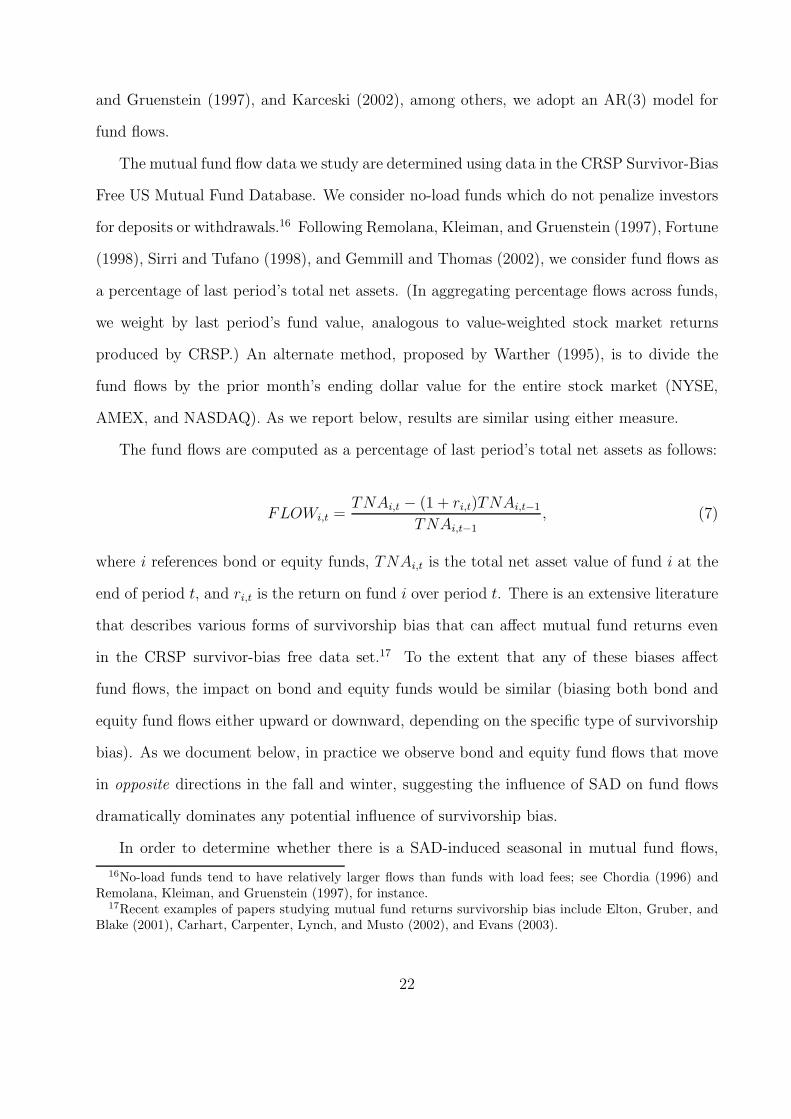
The mutual fund flow data we study are determined using data in the CRSP Survivor-Bias
Free US Mutual Fund Database. We consider no-load funds which do not penalize investors
for deposits or withdrawals.16 Following Remolana, Kleiman, and Gruenstein (1997), Fortune
(1998), Sirri and Tufano (1998), and Gemmill and Thomas (2002), we consider fund flows as
a percentage of last period’s total net assets. (In aggregating percentage flows across funds,
we weight by last period’s fund value, analogous to value-weighted stock market returns
produced by CRSP.) An alternate method, proposed by Warther (1995), is to divide the
fund flows by the prior month’s ending dollar value for the entire stock market (NYSE,
AMEX, and NASDAQ). As we report below, results are similar using either measure.
The fund flows are computed as a percentage of last period’s total net assets as follows:
FLOWi,t =TNAi,t − (1 + ri,t)TNAi,t−1
TNAi,t−1
, (7)
where i references bond or equity funds, TNAi,t is the total net asset value of fund i at the
end of period t, and ri,t is the return on fund i over period t. There is an extensive literature
that describes various forms of survivorship bias that can affect mutual fund returns even
in the CRSP survivor-bias free data set.17 To the extent that any of these biases affect
fund flows, the impact on bond and equity funds would be similar (biasing both bond and
equity fund flows either upward or downward, depending on the specific type of survivorship
bias). As we document below, in practice we observe bond and equity fund flows that move
in opposite directions in the fall and winter, suggesting the influence of SAD on fund flows
dramatically dominates any potential influence of survivorship bias.
In order to determine whether there is a SAD-induced seasonal in mutual fund flows,
16No-load funds tend to have relatively larger flows than funds with load fees; see Chordia (1996) andRemolana, Kleiman, and Gruenstein (1997), for instance.
17Recent examples of papers studying mutual fund returns survivorship bias include Elton, Gruber, andBlake (2001), Carhart, Carpenter, Lynch, and Musto (2002), and Evans (2003).
22
we select from the CRSP mutual fund database those funds which are either explicitly risk-
seeking in their investment objectives or inherently very safe. Our equity funds include only
those which state capital growth as an objective, permit short-selling, invest in unregistered
securities, allow borrowing up to 10 percent of the value of the portfolio, or invest at least 25
percent of the fund value in foreign securities. Based on these sorting criteria, we consider an
average of 1633 individual equity funds each month (ranging from a minimum of 436 funds
to a maximum of 2800). At the end of 2002, the total net asset value of the equity funds
we consider was 1.16 trillion dollars. The bond funds we consider are those which invest in
corporate bonds rated BBB or better or US government-backed securities (including Ginnie
Mae securities). The average number of bond funds in the resulting data set is 1010, with
a monthly minimum of 450 and a maximum of 1238. The total net asset value of the bond
funds we consider was 810 billion dollars at the end of 2002.18
In Table 8 we report summary statistics on the aggregate monthly fund flows for the bond
and equity mutual funds. As previously mentioned, fund flows are reported as a percentage
of the funds’ last period total net assets. The flow data we use span January 1992 through
December 2002. The mean monthly equity fund flow is 0.97 percent of the previous period’s
total equity fund value, while for bond funds the mean flow is 0.56 percent of the last
month’s bond fund value. The two flow series are similarly variable. The minimum and
maximum fund flows are similar across the fund categories at well under 10 percent in a
month, and both bond and equity fund flows display little skewness, but equity funds show
some leptokurtosis.
In Figure 4 we consider unconditional patterns in mutual fund flows. We plot the devi-
ation of the monthly average percentage flow from the annual average percentage flow for
each of equity mutual funds and bond mutual funds. Monthly bond flows, indicated with
an asterisk, rise sharply during autumn, peak in December, and then drop sharply in Jan-
18The CRSP codes for the equity mutual funds we consider are AG, GE, GI, IE, and LG, and the codes forthe bond funds we use are BQ, GS, GM, MG. CRSP obtains the monthly data from Investment CompanyData, Inc., now owned by Micropal.
23

uary through March. Monthly equity mutual fund flows, marked with solid dots, are below
average or declining in the fall and then they rise sharply in January and February. These
patterns are consistent with SAD-affected investors shifting their portfolios towards safer
assets in the fall, then back into risky assets in the winter.
To more formally investigate seasonal patterns in mutual fund flows, we consider the
following model:
FLOWi,t = µi + µi,SADSADt + µi,FallDFallt + µi,rri,t−1 (8)
+ ρi,1FLOWi,t−1 + ρi,2FLOWi,t−2 + ρi,3FLOWi,t−3 + εi,t,
where i references bond funds or equity funds, FLOWi,t is the month t fund flow expressed
as a percentage of last period’s total net assets, SADt is the SAD variable as defined in
Equation 3, DFallt is the fall dummy variable as defined in Equation 4, and ri,t−1 is the prior
month’s return to the set of funds (either the stock funds or the bond funds). Consistent
with prior studies, we include three lags of the dependent variable to control for autocorre-
lation. We estimate the models for bond fund flows and equity fund flows jointly in a GMM
framework and conduct inference using HAC covariance estimates.
Results of estimating Equation 8 are shown in Table 9. In Panel A of Table 9 we present
coefficient estimates, two-sided t-tests based on HAC standard errors, the value of R2 for
each estimation, and Lagrange Multiplier tests for up to 12 lags (a year) of autocorrelation
or ARCH. Considering the equity fund flows first, we find that the SAD coefficient estimate
is significantly positive and the fall estimate is significantly negative, consistent with risk
averse investors shunning risky assets in the fall and then resuming risky holdings as daylight
becomes more plentiful. The signs are reversed for the bond fund flows: the SAD coefficient
is significantly negative and the estimate on the fall dummy is significantly positive, again
consistent with what we expect.
In Panel B we present χ2 statistics for testing the joint significance of variables in the bond
24

and equity fund flow estimations. We strongly reject the hypothesis that the individually
significant SAD and fall coefficient estimates are jointly zero. We also strongly reject the
hypotheses that the SAD coefficients are equivalent across the bond and equity fund flow
estimations and that the fall coefficient estimates are the same across the two cases.
Relative to the average monthly mutual fund flows shown in Table 8 (around 1 percent
for equity funds and about half a percent for bond funds), the SAD-related flows (that is, the
SAD and fall coefficient estimates from Table 9) are of a comparable magnitude, as large as
three quarters of a percent for equity funds and up to almost a full percent for bond funds.
In Table 10 we present a detailed analysis of the economic significance of the fund flows due
to the SAD and fall variables.
In Panel A of Table 10 we translate the equity mutual fund flows into monetary flows
based on the aggregate December 2002 value of all the equity mutual funds we consider,
which is 1.16 trillion dollars. The value of the fall dummy in October, 1, multiplied by
the fall coefficient estimate, -0.752, yields the first value shown in the top line of the first
column. The value indicates that, all else constant, more than three quarters of a percent of
the equity mutual funds’ value flows out of equity mutual funds on average during October.
This represents an outflow exceeding 8 billion dollars, as shown in parentheses in the same
cell of the table. The economic impact of the fall variable is the same in each month of
the fall, and of course there is no impact in the winter months when the fall dummy equals
zero. The economic impact of the SAD variable is shown in the next column. Multiplying
the SAD coefficient from Table 9, 0.240, by the value of the SAD variable each month19
yields the set of figures shown on the left side of the SAD column. For instance, the value
of the SAD variable in October, 1.14, times the SAD coefficient of 0.240, equals 0.274. That
is, the average inflow of funds that can be attributed to the SAD variable that month, all
else constant, is over a quarter a percent of the value of equity funds. This represents more
19The value of the SAD variable, shown in Equation 3, during the fall and winter months is as follows:1.14 in October, 2.38 in November, 2.94 in December, 2.60 in January, 1.52 in February, and 0.13 in March.This is the median number of hours of night for each month, minus 12.
25

than three billion dollars, as shown in parentheses. The total net effect of the SAD and fall
variables is shown in the final column. For instance, the net outflow due to the fall variable
in October, -0.752 percent, plus the net inflow due to the SAD variable in October, 0.274
percent, yields a net outflow of -0.478 percent that month, which equates to over five billion
dollars net. Notice that the net effect of the fall and SAD variables is negative in all the fall
months and positive in all the winter months, consistent with our expectations.
Turning to Panel B, we can analyze the economic magnitude of the bond fund flows,
based on the December 2002 aggregate value of 809 billion dollars for the particular bond
funds we consider. The fall dummy coefficient estimate of 0.971 translates into over 7 billion
dollars in monthly flows into bond funds during October, November, and December. The
economic impact of the SAD variable alone varies from under a billion dollars to over five
billion dollars in average monthly outflows. The net effect of the fall and SAD variables
is positive during the fall months and negative during the winter months, again, consistent
with our expectations.
Overall, the evidence suggests that when funds are flowing out of equity funds, they are
flowing into bond funds. For instance in October, the SAD/fall-related flow out of equity
funds is $5.55 billion, while the flow into bond funds is $5.83 billion. Similarly, when funds
are flowing into equity funds, they are flowing out of bond funds.
In further robustness checks, we explored the impact of various modifications to the
estimation model. We explored both the inclusion of contemporaneous market returns or
fund returns as a regressor,20 the inclusion of lagged market returns as a regressor, and
the more parsimonious model excluding any return variable as a regressor, and we found
virtually identical results. Warther (1995) found that money market funds, but not other
funds, display significant outflows in December and inflows in January. While we don’t
focus on money market funds, we still investigated whether similar patterns might drive our
results for bond and equity fund flows by including December and January dummy variables
20Note that there can be an endogeneity problem in using contemporaneous returns in the regression.
26

as additional regressors. In all cases, we found standard errors, coefficient estimates, and
significance of the SAD and fall variables to be very similar to those we report in this paper.
Details on all the robustness checks are available from the authors on request.
6 Conclusions
The medical literature is unequivocal that Seasonal Affective Disorder is a serious emotional
condition that afflicts millions of people during the seasons when daylight is scarce. The
depression associated with SAD in turn affects the willingness to seek sensation, that is, to
engage in activities involving risk. It is therefore not surprising that SAD permeates capital
markets, which are risky by nature. To date, only the stock market has been studied (KKL
2003) where it has been shown that market indices move with the cycle of light and dark
that accompanies the revolution of the Earth around the Sun.
In this paper, we have shown that the seasonal regularities go well beyond equity markets.
First, we have documented a cycle in bond returns that is the converse of the SAD stock
market return cycle. Just as autumn stock returns tend to drop with increasing length of
night, so at the same time bond returns tend to rise. Then as the hours of night cycle
moves through its maximum, around December 21, and the days lengthen towards spring,
stock returns rise and bond returns drop. These inverted patterns are both statistically and
economically significant, and they occur in spite of strong positive correlation between our
monthly bond index returns and stock index returns.
Second, this paper has also shown that the cyclical regularities in equities are highest in
riskier segments of the stock market. Whether we sort stock portfolios by beta or standard
deviation of return, the riskier the decile the higher in almost every instance is the amplitude
of the return cycle. This is consistent with SAD-affected investors showing greater aversion
to holding risky stocks versus safe stocks in the fall and then showing greater inclination to
hold risky stocks versus safe stocks in the new year. Finally, when we examine the movement
of funds within the capital market by viewing the flows of money between different classes
27

of mutual funds during the fall and winter, we find that money moves out of stocks and into
bonds in fall as the days shorten. The flow is reversed in the new year as the days lengthen.
Not only are the cyclical indicators statistically significant for the flows between different
types of funds we consider, even the flows into the safer (riskier) funds correspond closely to
the amounts flowing out of the riskier (safer) funds. This is the annual cycle in fund flows
that seasonal patterns in daylight and SAD-related risk aversion would suggest.
It should also be recalled that we consider seasonal variation in the willingness to accept
risk, not seasonal variation in risk itself. Previous studies of seasonality in risk premia
consider patterns, including those around the turn of the year, as being the result of variations
in the risk of the securities. For example, Keim and Stambaugh (1986) suggest that risk may
drop at the turn of the year, pointing out that de-listings of stocks in the 1927-81 period
were most frequent during December and least frequent during January. Indeed, they write
on page 359, “The seasonality ... might suggest a tendency for increased risk around the
turn of the year.” Of course, it is difficult to distinguish perceptions of risk from willingness
to accept risk. Both cause an increase in measured risk premia. It might be argued, however,
that if a seasonal influence moves relatively predictably through fall and winter in a pattern
that corresponds to the fluctuations in daylight, it is unlikely that smooth variations in
risk through the course of the year is responsible. Just as SAD is widely accepted as a
serious emotional condition that influences the general population, this paper has shown
that investors are no different. This should not be a surprise. After all, investors are human.
28

References
Bergstresser, Daniel and James Poterba. Do after-tax returns affect mutual fund inflows?Journal of Financial Economics, 2002, 63, 381-414.
Carhart, Mark M., Jennifer N. Carpenter, Anthony W. Lynch, and David K. Musto. MutualFund Survivorship. Review of Financial Studies, Winter 2002, 15(5), 1439-1463.
Carton, Solange, Roland Jouvent, Catherine Bungener, and D. Widlocher. Sensation Seekingand Depressive Mood. Personality and Individual Differences, July 1992, 13(7), 843-849.
Chang, Eric C. and Roger D. Huang, Time-Varying Return and Risk in the Corporate BondMarket, Journal of Financial and Quantitative Analysis, September 1990, 25(3) 323-340.
Chordia, Tarun. The structure of mutual fund charges. Journal of Financial Economics,1996, 41, 3-39.
Cohen, Robert M., M. Gross, Thomas E. Nordahl, W.E. Semple, D.A. Oren, and Norman E.Rosenthal. Preliminary Data on the Metabolic Brain Pattern of Patients with WinterSeasonal Affective Disorder. Archives of General Psychiatry, July 1992, 49(7), 545-552.
Del Guercio, Diane, and Paula A. Tkac. The Effect of Morningstar Ratings on Mutual FundFlows. Mimeo, Federal Reserve Bank of Atlanta, GA, 2001.
Delgado, Pedro L. Depression: The Case for a Monoamine Deficiency. Journal of ClinicalPsychiatry, 2000, 61 Suppl. 6, 7-11.
Edwards, Franklin R. and Xin Zhang. Mutual Funds and Stock and Bond Market Stability.Journal of Financial Services Research, 1998, 13(3), 257-282.
Eisenberg, Amy E., Jonathan Baron, and Martin E.P. Seligman. Individual Differencesin Risk Aversion and Anxiety. Mimeo, University of Pennsylvania Department ofPsychology, 1998.
Elton, Edwin J., Martin J. Gruber, and Christopher R. Blake. A First Look at the Accuracyof the CRSP Mutual Fund Database and a Comparison of the CRSP and MorningstarMutual Fund Databases. Journal of Finance, December 2001, 61(6), 257-282.
Evans, Richard B. Mutual Fund Incubation and Termination: The Endogeneity of Survivor-ship Bias. Wharton School of Business Manuscript, April 2003.
Faedda, Gianni L., Leonardo Tondo, M.H. Teicher, Ross J. Baldessarini, H.A. Gelbard, andG.F. Floris. Seasonal Mood Disorders, Patterns in Mania and Depression. Archivesof General Psychiatry, 1993, 50, 17-23.
Fama, Eugene F. and Kenneth R. French. The Cross-Section of Expected Returns. Journalof Finance, June 1992, 47(2), 427-465.
Fortune, Peter. Mutual Funds, Part II: Fund Flows and Security Returns. New EnglandEconomic Review, January/February 1998, 47(2), 3-22.
29

Gemmill, Gordon and Dylan C. Thomas. Noise Trading, Costly Arbitrage, and Asset Prices:Evidence from Closed-end Funds. Journal of Finance, December 2002, 57(6) 2571-2594.
Granger, Clive. Investigating Causal Relations by Econometric Models and Cross SpectralMethods. Econometrica, April 1969, 37, 424-438.
Hansen, Lars Peter. Large Sample Properties of Generalized Method of Moments Estimators.Econometrica, 1982, 50, 1029-1054.
Harlow, W.V. and Keith C. Brown. Understanding and Assessing Financial Risk Tolerance:A Biological Perspective, Financial Analysts Journal, November-December 1990, 50-80.
Hirschfeld, Robert M.A. History and Evolution of the Monoamine Hypothesis of Depression,Journal of Clinical Psychiatry, 2000, 61 Suppl. 6, 4-6.
Horvath, Paula and Marvin Zuckerman. Sensation Seeking, Risk Appraisal, and RiskyBehavior. Personality and Individual Differences, January 1993, 14(1), 41-52.
Investment Company Institute. Mutual Fund Fact Book: A Guide to Trends and Statisticsin the Mutual Fund Industry, 42nd Edition, 2002.
Investment Company Institute and the Security Industry Association. Equity Ownership inAmerica, 2002.
Ippolito, Richard A. Consumer reaction to measures of poor quality: Evidence from themutual fund industry. Journal of Law and Economics, 1992, 35, 45-70.
Jordan, Susan D. and Bradford D. Jordan, Seasonality in Daily Bond Returns, Journal ofFinancial and Quantitative Analysis, June 1991, 26(2) 269-285.
Kamstra, Mark J., Lisa A. Kramer, and Maurice D. Levi, Winter Blues: A SAD StockMarket Cycle, American Economic Review, March 2003, 93(1) 324-343.
Karceski, Jason. Returns-Chasing Behavior, Mutual Funds, and Beta’s Death. Journal ofFinancial and Quantitative Analysis, December 2002, 37(4) 559-594.
Keim, Donald B. Size-related Anomalies and Stock Return Seasonality: Further EmpiricalEvidence. Journal of Financial Economics, June 1983, 12(1), 13-32.
Keim, Donald B. and Robert F. Stambaugh. Predicting Returns in the Stock and BondMarkets. Journal of Financial Economics, December 1986, 17(2), 357-390.
Kothari, S.P., Jay Shanken, and Richard G. Sloan. Another Look at the Cross-Section ofExpected Stock Returns. Journal of Finance, March 1995, 50(1), 185-224.
Lam, Raymond W., Ed., Seasonal Affective Disorder and Beyond: Light Treatment for SADand Non-SAD Conditions, Washington DC: American Psychiatric Press, 1998.
Molin, Jeanne, Erling Mellerup, Tom Bolwig, Thomas Scheike, and Henrik Dam. The Influ-ence of Climate on Development of Winter Depression. Journal of Affective Disorders,April 1996, 37(2-3), 151-155.
Newey, Whitney K. and Kenneth D. West. A Simple, Positive, Semi-Definite, Heteroscedas-ticity and Autocorrelation Consistent Covariance Matrix, Econometrica, 1987, 55,703-708.
30

Reiganum, Marc R. The Anomalous Stock Market Behavior of Small Firms in January.Journal of Financial Economics, June 1983, 12(1), 89-104.
Remolana, Eli M., Paul Kleiman and Debbie Gruenstein. Market Returns and Mutual FundFlows. Federal Reserve Bank of New York Economic Policy Review, July 1997, 33-52.
Ritter, Jay R. The Buying and Selling Behavior of Individual Investors at the Turn of theYear. Journal of Finance, July 1988, 43(3), pp. 701-717.
Roll, Richard. Vas Ist Das? The Turn of the Year Effect and the Return Premia of SmallFirms. Journal of Portfolio Management, Winter 1983, 9, 18-28.
Rogalski, Richard J. and Seha M. Tinic. The January Size Effect: Anomaly or Risk Mis-measurement? Mimeo, Dartmouth College, NH, 1984.
Rosenthal, Norman E. Winter Blues: Seasonal Affective Disorder: What is It and How toOvercome It, 2nd Edition. New York: Guilford Press, 1998.
Schneeweis, Thomas and J. Randall Woolridge. Capital Market Seasonality: The Case ofBond Returns, Journal of Financial and Quantitative Analysis, December 1979, 14(5)939-958.
Sirri, Erik R. and Peter Tufano. Costly Search and Mutual Fund Flows. Journal of Finance,October 1998, 53(5), 1589-1622.
Telser, Lester G. A Critique of Some Recent Empirical Research on the Explanation of theTerm Structure of Interest Rates, Journal of Political Economy, August 1967, 75(4),Part 2, 546-561.
Thaler, Richard H. Anomalies: The January Effect. Journal of Economic Perspectives,Summer 1987, 1(1), 197-201.
Warther, Vincent A. Aggregate mutual fund flows and security returns. Journal of FinancialEconomics, 1995, 39, 209-235.
Wilson, Jack W. and Charles P. Jones. Is There a January Effect in Corporate Bond andPaper Returns? Financial Review, 1990, 25(1) 55-71.
Wong, Alan and Bernardo Carducci. Sensation Seeking and Financial Risk Taking in Ev-eryday Money Matters. Journal of Business and Psychology, Summer 1991, 5(4),525-530.
Young, Michael A., Patricia M. Meaden, Louis F. Fogg, Eva A. Cherin, and CharmaneI. Eastman. Which Environmental Variables are Related to the Onset of SeasonalAffective Disorder? Journal of Abnormal Psychology, November 1997, 106(4), 554-562.
Zuckerman, Marvin, Monte S. Buchsbaum, and Dennis L. Murphy. Sensation Seeking andits Biological Correlates. Psychological Bulletin, January 1980, 88(1), 187-214.
Zuckerman, Marvin. Biological Bases of Sensation Seeking, Impulsivity and Anxiety. Hills-dale, NJ: Lawrence Erlbaum Associates, Inc., 1983.
Zuckerman, Marvin. Sensation Seeking: A Comparative Approach to a Human Trait. Be-havioral and Brain Science, 1984, 7, 413-471.
31

Table 1: Summary Statistics On Bond Index Percentage Returns
We present summary statistics on monthly US government bond index returns obtained from CRSP.For each bond index return series we present the number of observations (N), mean percentagereturn (Mean), standard deviation (Std), minimum (Min), maximum (Max), skewness (Skew) andkurtosis (Kurt). The start and end dates for each series are presented beneath the series names.
Monthly Government Bond IndicesStart Date - End Date N Mean Std Min Max Skew Kurt
10 year Govt. Bond Index 728 0.455 1.96 -6.67 10.00 0.682 2.711941-05 - 2001-12
7 year Govt. Bond Index 729 0.479 1.64 -7.04 10.75 0.879 5.631941-04 - 2001-12
5 year Govt. Bond Index 729 0.470 1.38 -5.80 10.61 0.843 6.651941-04 - 2001-12
2 year Govt. Bond Index 732 0.447 0.81 -3.69 8.42 2.070 18.561941-01 - 2001-12
1 year Govt. Bond Index 732 0.440 0.53 -1.72 5.61 2.468 16.901941-01 - 2001-12
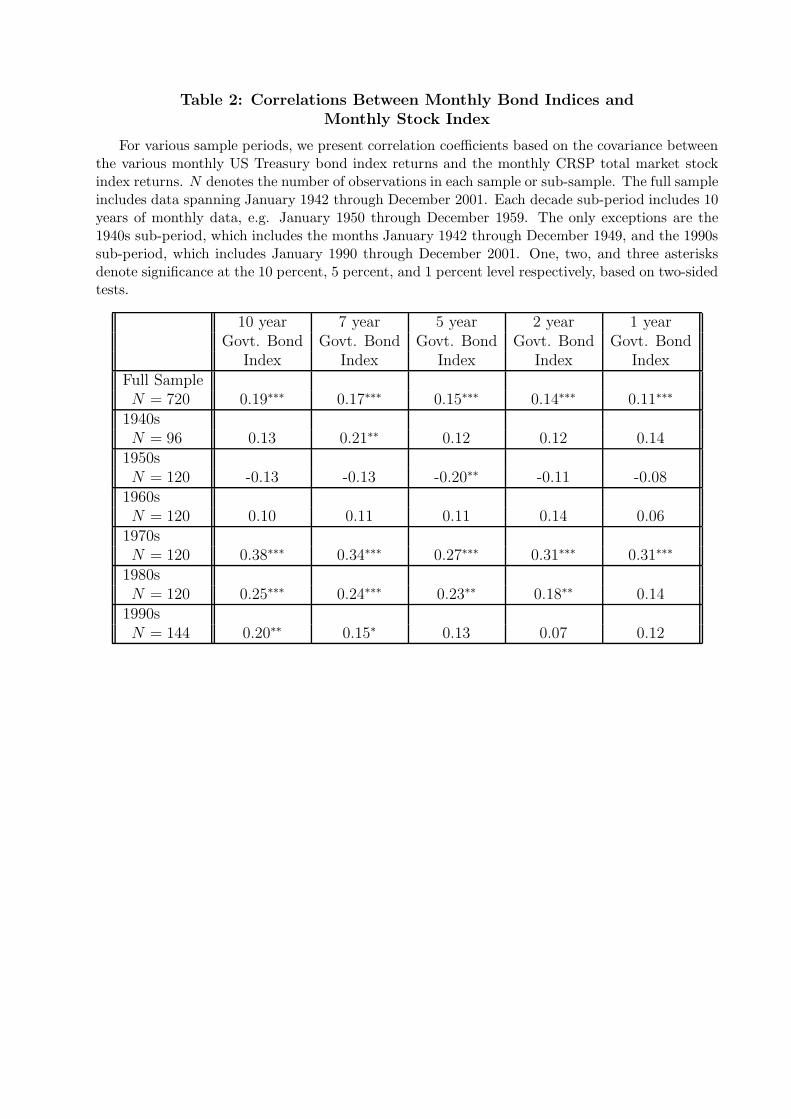
Table 2: Correlations Between Monthly Bond Indices andMonthly Stock Index
For various sample periods, we present correlation coefficients based on the covariance betweenthe various monthly US Treasury bond index returns and the monthly CRSP total market stockindex returns. N denotes the number of observations in each sample or sub-sample. The full sampleincludes data spanning January 1942 through December 2001. Each decade sub-period includes 10years of monthly data, e.g. January 1950 through December 1959. The only exceptions are the1940s sub-period, which includes the months January 1942 through December 1949, and the 1990ssub-period, which includes January 1990 through December 2001. One, two, and three asterisksdenote significance at the 10 percent, 5 percent, and 1 percent level respectively, based on two-sidedtests.
10 year 7 year 5 year 2 year 1 yearGovt. Bond Govt. Bond Govt. Bond Govt. Bond Govt. Bond
Index Index Index Index IndexFull SampleN = 720 0.19∗∗∗ 0.17∗∗∗ 0.15∗∗∗ 0.14∗∗∗ 0.11∗∗∗
1940sN = 96 0.13 0.21∗∗ 0.12 0.12 0.14
1950sN = 120 -0.13 -0.13 -0.20∗∗ -0.11 -0.08
1960sN = 120 0.10 0.11 0.11 0.14 0.06
1970sN = 120 0.38∗∗∗ 0.34∗∗∗ 0.27∗∗∗ 0.31∗∗∗ 0.31∗∗∗
1980sN = 120 0.25∗∗∗ 0.24∗∗∗ 0.23∗∗ 0.18∗∗ 0.14
1990sN = 144 0.20∗∗ 0.15∗ 0.13 0.07 0.12

Table 3: Regression Results forMonthly Government Bond Index Returns
We report coefficient estimates from jointly estimating the following expression for each of themonthly government bond indices in a GMM framework:
ri,t = µi + ρi,1ri,t−1 + µi,SADSADt + µi,FallDFallt + µi,TaxDTax
t + εi,t. (5)
Bond index returns (ri,t, where i indicates the category of bond maturities) are regressed on aconstant (µ), lagged returns, the SAD measure (SADt = Ht−12 during fall and winter, 0 otherwise,where Ht = median monthly number of hours of night), a dummy for months in the fall (DFall
t ),and a tax-loss selling dummy for the month of January (DTax
t ).In Panel A we present parameter estimates, with associated t-statistics below, calculated using
Newey and West (1987) HAC standard errors. At the bottom of Panel A, we present the value ofR2 for each index, as well as Lagrange Multiplier χ2 test statistics for the presence of up to a year,12 lags, of autocorrelation (AR) or ARCH. In Panel B we present Wald χ2 tests, with degrees offreedom in square brackets, for testing the equivalence of the SAD and fall coefficient estimates tozero. Two and three asterisks denote significance at the 5 percent and 1 percent levels respectively,based on two-sided tests.
Panel A: Parameter Estimates, T-tests, and DiagnosticsParameter 10 year 7 year 5 year 2 year 1 yearµ 0.318∗∗∗ 0.356∗∗∗ 0.347∗∗∗ 0.293∗∗∗ 0.239∗∗∗
( 5.761) ( 7.996) ( 9.728) ( 14.016) ( 16.129)ρ1 0.096∗∗∗ 0.118∗∗∗ 0.147∗∗∗ 0.261∗∗∗ 0.408∗∗∗
( 6.537) ( 9.415) ( 12.355) ( 22.702) ( 34.881)µSAD -0.181∗∗ -0.169∗∗∗ -0.158∗∗∗ -0.093∗∗∗ -0.073∗∗∗
( -2.251) ( -2.693) ( -3.122) ( -3.698) ( -4.978)µFall 0.563∗∗∗ 0.541∗∗∗ 0.436∗∗∗ 0.247∗∗∗ 0.175∗∗∗
( 2.947) ( 3.621) ( 3.484) ( 3.929) ( 4.721)µTax 0.684∗∗ 0.417∗∗ 0.496∗∗∗ 0.374∗∗∗ 0.286∗∗∗
( 2.541) ( 2.115) ( 3.061) ( 4.767) ( 6.083)R2 0.0159 0.0221 0.0287 0.0737 0.1692AR(12) 17.21 17.78 21.84∗∗ 59.82∗∗∗ 128.96∗∗∗
ARCH(12) 126.28∗∗∗ 101.86∗∗∗ 92.58∗∗∗ 63.89∗∗∗ 85.46∗∗∗
Panel B: Joint TestTest: χ2 [degrees of freedom]SAD and fall coefficients jointly zero across series 42.4∗∗∗ [10]

Table 4: Average Annual Percentage ReturnDue to SAD and Due to Fall Dummy
for Government Bond Indices
For each of the monthly government bond series (1, 2, 5, 7, and 10 year maturities, dataobtained from CRSP), we report the total average annual percentage return, the average annualpercentage return due to the SAD variable, and the average annual percentage return due to thefall variable. In calculating the average annual return due to SAD for a particular index, we takethe value of the SAD variable for each month, multiply by the index’s SAD variable estimate fromTable 3, average across months, and then adjust the outcome to obtain an annualized percentagereturn. Similarly, in calculating the annual average return due to the fall dummy for a particularindex, we take that index’s fall dummy variable estimate from Table 3, multiply by the value of thefall dummy variable (one during periods in the fall, zero otherwise), average across months, andthen adjust the result to obtain an annualized percentage return. Two and three asterisks denotesignificance at the 5 percent and 1 percent levels respectively, based on two-sided tests. In the caseof the columns for the annualized returns due to the SAD and fall dummy variables, significance isbased on t-tests on the parameter estimates from Table 3. In the case of the unconditional returncolumn, significance is based on t-tests for a mean daily return different from zero.
Average AverageTotal Average Annual Return Annual Return
Monthly Government Annual Due to Due toBond Indices Return (%) SAD Variable (%) Fall Variable (%)10 year 5.59∗∗∗ -1.920∗∗ 1.700∗∗∗
7 year 5.89∗∗∗ -1.800∗∗∗ 1.630∗∗∗
5 year 5.79∗∗∗ -1.680∗∗∗ 1.310∗∗∗
2 year 5.58∗∗∗ -0.990∗∗∗ 0.740∗∗∗
1 year 5.49∗∗∗ -0.780∗∗∗ 0.530∗∗∗

Table 5: Summary Statistics on Daily CRSP Decile Returns
The summary statistics reported in this table are based on beta-sorted CRSP decile returns(Panel A) and volatility-sorted CRSP decile returns (Panel B). The daily data span the periodJuly 3, 1962 through December 31, 2001, for which there are 9942 observations. Decile 1 containsthe 10 percent of firms with the largest beta or return standard deviation while decile 10 containsfirms with the smallest beta or return standard deviation. For each decile return series we presentthe mean percentage return (Mean), standard deviation (Std), minimum (Min), maximum (Max),skewness (Skew) and kurtosis (Kurt).
Panel A: Beta-Sorted DecilesDecile Mean Std Min Max Skew Kurt1 0.092 1.34 -19.83 14.77 -0.234 11.952 0.076 1.10 -17.86 11.82 -0.519 14.523 0.079 0.98 -17.35 10.20 -0.707 16.884 0.079 0.90 -16.74 11.59 -0.755 21.425 0.076 0.82 -14.85 9.96 -0.819 19.926 0.078 0.74 -12.88 7.95 -0.788 16.607 0.079 0.68 -12.52 9.48 -0.869 23.508 0.078 0.60 -11.47 7.35 -1.043 24.279 0.077 0.53 -10.06 7.64 -0.838 27.5810 0.111 0.59 -9.00 8.82 -0.656 24.12
Panel B: Standard-Deviation-Sorted DecilesDecile Mean Std Min Max Skew Kurt1 0.181 1.18 -14.36 15.00 0.309 13.932 0.071 1.06 -15.36 11.96 -0.428 14.863 0.062 0.99 -15.74 12.29 -0.589 17.034 0.066 0.89 -14.42 9.93 -0.743 17.045 0.067 0.81 -13.99 8.90 -0.944 18.656 0.064 0.75 -14.49 8.62 -1.119 21.687 0.061 0.69 -14.82 8.19 -1.268 29.738 0.059 0.62 -14.47 8.34 -1.449 38.949 0.054 0.53 -12.98 8.16 -1.492 49.2110 0.048 0.40 -9.72 5.70 -1.418 46.31

Table 6: Regression Results for Daily CRSP Decile Returns
We report coefficient estimates from jointly estimating, in a GMM framework, the followingregression using as the dependent variable each of the beta-sorted CRSP decile returns (Panel A)and standard-deviation-sorted CRSP decile returns (Panel B).
ri,t = µi + µi,SADSADt + µi,FallDFallt + µi,MonDMon
t + µi,TaxDTaxt + εi,t (6)
For each decile i = 1, · · · , 10, decile returns (ri,t) are regressed on a constant (µ); the SADmeasure (SADt = Ht − 12 during fall and winter, 0 otherwise, where Ht = number of hours ofnight); a dummy for trading days in the fall (DFall
t ); a dummy for trading days following theweekend (DMon
t ); and a dummy for the last trading day of December and the first five tradingdays of January (DTax
t ). Decile 1 contains the 10 percent of firms with the largest beta or returnstandard deviation while decile 10 contains firms with the smallest beta or standard deviation.
We present parameter estimates, with associated t-statistics in parentheses below, calculatedusing Newey and West (1987) HAC standard errors. At the bottom of each table, we present thevalue of R2 for each estimation, as well as Lagrange Multiplier χ2 test statistics for the presenceof up to a month, 20 lags, of autocorrelation (AR) or ARCH. We also present Wald χ2 tests, withtheir degrees of freedom in square brackets and their p-values below in parentheses, for testingthe equivalence of the SAD and fall coefficient estimates to zero (joint test 1), and for testing thejoint equality of the SAD and fall coefficient estimates respectively (joint tests 2 and 3) across thebond return series. Two and three asterisks denote significance at the 5 percent and 1 percent levelrespectively, based on two-sided tests.
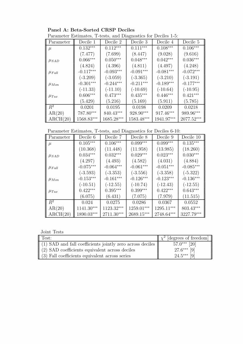
Panel A: Beta-Sorted CRSP DecilesParameter Estimates, T-tests, and Diagnostics for Deciles 1-5:Parameter Decile 1 Decile 2 Decile 3 Decile 4 Decile 5µ 0.132∗∗∗ 0.112∗∗∗ 0.111∗∗∗ 0.108∗∗∗ 0.106∗∗∗
(7.477) (7.699) (8.447) (9.028) (9.616)µSAD 0.066∗∗∗ 0.050∗∗∗ 0.048∗∗∗ 0.042∗∗∗ 0.036∗∗∗
(4.824) (4.396) (4.811) (4.497) (4.248)µFall -0.117∗∗∗ -0.093∗∗∗ -0.091∗∗∗ -0.081∗∗∗ -0.072∗∗∗
(-3.209) (-3.059) (-3.365) (-3.210) (-3.191)µMon -0.301∗∗∗ -0.244∗∗∗ -0.211∗∗∗ -0.189∗∗∗ -0.177∗∗∗
(-11.33) (-11.10) (-10.69) (-10.64) (-10.95)µTax 0.606∗∗∗ 0.473∗∗∗ 0.435∗∗∗ 0.446∗∗∗ 0.421∗∗∗
(5.429) (5.216) (5.169) (5.911) (5.785)R2 0.0201 0.0195 0.0198 0.0209 0.0218AR(20) 787.80∗∗∗ 840.43∗∗∗ 928.90∗∗∗ 917.46∗∗∗ 989.96∗∗∗
ARCH(20) 1568.83∗∗∗ 1685.28∗∗∗ 1583.48∗∗∗ 1941.97∗∗∗ 2077.52∗∗∗
Parameter Estimates, T-tests, and Diagnostics for Deciles 6-10:Parameter Decile 6 Decile 7 Decile 8 Decile 9 Decile 10µ 0.105∗∗∗ 0.106∗∗∗ 0.099∗∗∗ 0.099∗∗∗ 0.135∗∗∗
(10.368) (11.448) (11.958) (13.985) (18.260)µSAD 0.034∗∗∗ 0.032∗∗∗ 0.029∗∗∗ 0.023∗∗∗ 0.030∗∗∗
(4.297) (4.493) (4.582) (4.031) (4.884)µFall -0.075∗∗∗ -0.064∗∗∗ -0.061∗∗∗ -0.051∗∗∗ -0.085∗∗∗
(-3.593) (-3.353) (-3.556) (-3.358) (-5.322)µMon -0.153∗∗∗ -0.161∗∗∗ -0.126∗∗∗ -0.123∗∗∗ -0.136∗∗∗
(-10.51) (-12.55) (-10.74) (-12.43) (-12.55)µTax 0.422∗∗∗ 0.395∗∗∗ 0.399∗∗∗ 0.422∗∗∗ 0.643∗∗∗
(6.075) (6.431) (7.075) (7.979) (11.515)R2 0.024 0.0275 0.0286 0.0367 0.0552AR(20) 1141.30∗∗∗ 1123.32∗∗∗ 1259.01∗∗∗ 1295.11∗∗∗ 803.43∗∗∗
ARCH(20) 1890.03∗∗∗ 2711.30∗∗∗ 2689.15∗∗∗ 2748.64∗∗∗ 3227.79∗∗∗
Joint TestsTest: χ2 [degrees of freedom](1) SAD and fall coefficients jointly zero across deciles 57.0∗∗∗ [20](2) SAD coefficients equivalent across deciles 27.6∗∗∗ [9](3) Fall coefficients equivalent across series 24.5∗∗∗ [9]

Panel B: Standard-Deviation-Sorted CRSP DecilesParameter Estimates, T-tests, and Diagnostics for Deciles 1-5:Parameter Decile 1 Decile 2 Decile 3 Decile 4 Decile 5µ 0.215∗∗∗ 0.122∗∗∗ 0.106∗∗∗ 0.104∗∗∗ 0.098∗∗∗
(14.886) (9.099) (8.360) (9.016) (9.031)µSAD 0.074∗∗∗ 0.051∗∗∗ 0.049∗∗∗ 0.045∗∗∗ 0.042∗∗∗
(5.944) (4.609) (4.776) (4.865) (4.906)µFall -0.207∗∗∗ -0.142∗∗∗ -0.115∗∗∗ -0.104∗∗∗ -0.088∗∗∗
(-6.500) (-4.948) (-4.233) (-4.239) (-3.861)µMon -0.369∗∗∗ -0.309∗∗∗ -0.249∗∗∗ -0.211∗∗∗ -0.175∗∗∗
(-17.16) (-15.20) (-13.09) (-12.18) (-10.99)µTax 1.364∗∗∗ 0.718∗∗∗ 0.454∗∗∗ 0.341∗∗∗ 0.256∗∗∗
(10.052) (7.337) (5.444) (4.438) (3.828)R2 0.0802 0.0411 0.027 0.0228 0.0183AR(20) 1058.98∗∗∗ 939.12∗∗∗ 926.60∗∗∗ 1009.34∗∗∗ 1123.12∗∗∗
ARCH(20) 2051.47∗∗∗ 2117.56∗∗∗ 2465.95∗∗∗ 2335.15∗∗∗ 2292.26∗∗∗
Parameter Estimates, T-tests, and Diagnostics for Deciles 6-10:Parameter Decile 6 Decile 7 Decile 8 Decile 9 Decile 10µ 0.093∗∗∗ 0.085∗∗∗ 0.081∗∗∗ 0.071∗∗∗ 0.059∗∗∗
(9.201) (9.269) (9.669) (10.053) (10.620)µSAD 0.036∗∗∗ 0.030∗∗∗ 0.023∗∗∗ 0.017∗∗∗ 0.009∗∗
(4.535) (4.117) (3.623) (3.073) (2.118)µFall -0.076∗∗∗ -0.059∗∗∗ -0.049∗∗∗ -0.031∗∗ -0.016
(-3.635) (-3.074) (-2.837) (-2.107) (-1.396)µMon -0.147∗∗∗ -0.122∗∗∗ -0.104∗∗∗ -0.087∗∗∗ -0.059∗∗∗
(-9.893) (-8.951) (-8.528) (-8.600) (-7.789)µTax 0.191∗∗∗ 0.163∗∗∗ 0.122∗∗ 0.136∗∗∗ 0.147∗∗∗
(3.092) (2.834) (2.376) (3.032) (4.183)R2 0.0148 0.0121 0.0104 0.0114 0.0126AR(20) 1106.09∗∗∗ 1118.05∗∗∗ 1116.94∗∗∗ 1250.94∗∗∗ 1577.62∗∗∗
ARCH(20) 1811.10∗∗∗ 1498.09∗∗∗ 1635.72∗∗∗ 1682.51∗∗∗ 1208.69∗∗∗
Joint TestsTest: χ2 [degrees of freedom](1) SAD and fall coefficients jointly zero across deciles 81.4∗∗∗ [20](2) SAD coefficients equivalent across deciles 51.0∗∗∗ [9](3) Fall coefficients equivalent across series 57.9∗∗∗ [9]
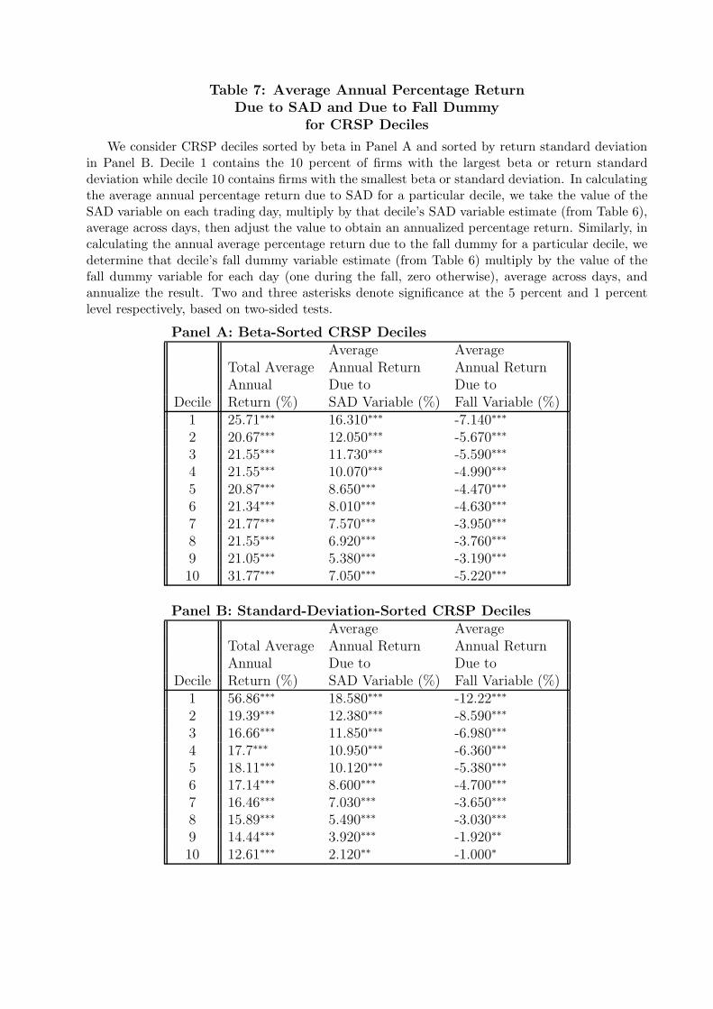
Table 7: Average Annual Percentage ReturnDue to SAD and Due to Fall Dummy
for CRSP Deciles
We consider CRSP deciles sorted by beta in Panel A and sorted by return standard deviationin Panel B. Decile 1 contains the 10 percent of firms with the largest beta or return standarddeviation while decile 10 contains firms with the smallest beta or standard deviation. In calculatingthe average annual percentage return due to SAD for a particular decile, we take the value of theSAD variable on each trading day, multiply by that decile’s SAD variable estimate (from Table 6),average across days, then adjust the value to obtain an annualized percentage return. Similarly, incalculating the annual average percentage return due to the fall dummy for a particular decile, wedetermine that decile’s fall dummy variable estimate (from Table 6) multiply by the value of thefall dummy variable for each day (one during the fall, zero otherwise), average across days, andannualize the result. Two and three asterisks denote significance at the 5 percent and 1 percentlevel respectively, based on two-sided tests.
Panel A: Beta-Sorted CRSP DecilesAverage Average
Total Average Annual Return Annual ReturnAnnual Due to Due to
Decile Return (%) SAD Variable (%) Fall Variable (%)1 25.71∗∗∗ 16.310∗∗∗ -7.140∗∗∗
2 20.67∗∗∗ 12.050∗∗∗ -5.670∗∗∗
3 21.55∗∗∗ 11.730∗∗∗ -5.590∗∗∗
4 21.55∗∗∗ 10.070∗∗∗ -4.990∗∗∗
5 20.87∗∗∗ 8.650∗∗∗ -4.470∗∗∗
6 21.34∗∗∗ 8.010∗∗∗ -4.630∗∗∗
7 21.77∗∗∗ 7.570∗∗∗ -3.950∗∗∗
8 21.55∗∗∗ 6.920∗∗∗ -3.760∗∗∗
9 21.05∗∗∗ 5.380∗∗∗ -3.190∗∗∗
10 31.77∗∗∗ 7.050∗∗∗ -5.220∗∗∗
Panel B: Standard-Deviation-Sorted CRSP DecilesAverage Average
Total Average Annual Return Annual ReturnAnnual Due to Due to
Decile Return (%) SAD Variable (%) Fall Variable (%)1 56.86∗∗∗ 18.580∗∗∗ -12.22∗∗∗
2 19.39∗∗∗ 12.380∗∗∗ -8.590∗∗∗
3 16.66∗∗∗ 11.850∗∗∗ -6.980∗∗∗
4 17.7∗∗∗ 10.950∗∗∗ -6.360∗∗∗
5 18.11∗∗∗ 10.120∗∗∗ -5.380∗∗∗
6 17.14∗∗∗ 8.600∗∗∗ -4.700∗∗∗
7 16.46∗∗∗ 7.030∗∗∗ -3.650∗∗∗
8 15.89∗∗∗ 5.490∗∗∗ -3.030∗∗∗
9 14.44∗∗∗ 3.920∗∗∗ -1.920∗∗
10 12.61∗∗∗ 2.120∗∗ -1.000∗

Table 8: Summary Statistics on Percentage Mutual Fund Flows
We present summary statistics on monthly mutual fund flows for a total of 132 months usingdata provided by CRSP. The CRSP codes for the equity mutual funds we consider are AG, GE,GI, IE, and LG, and the codes for the bond funds we use are BQ, GS, GM, MG. The flows arecomputed as FLOWi,t = TNAi,t−(1+ri,t)TNAi,t−1
TNAi,t−1, where the i index references bond or equity funds,
TNAi,t is the total net asset value of fund i at the end of period t, and ri,t−1 is the return on fundi over period t. For each set of fund flows we present the number of monthly observations (N), themean monthly flow (Mean), standard deviation (Std), minimum (Min), maximum (Max), skewness(Skew) and kurtosis (Kurt). Details on the number of individual funds available in these categorieseach month are as follows: for equity funds the minimum is 436, the maximum is 2800, and themean is 1633; for bond funds the minimum is 450, the maximum is 1238, and the mean is 1010.
Mutual Fund Data SetStart Date - End Date N Mean Std Min Max Skew Kurt
Equity 132 0.972 1.06 -4.54 5.83 -0.081 7.611992-01-31 - 2002-12-31
Bonds 132 0.557 1.44 -3.33 6.47 0.316 1.991992-01-31 - 2002-12-31
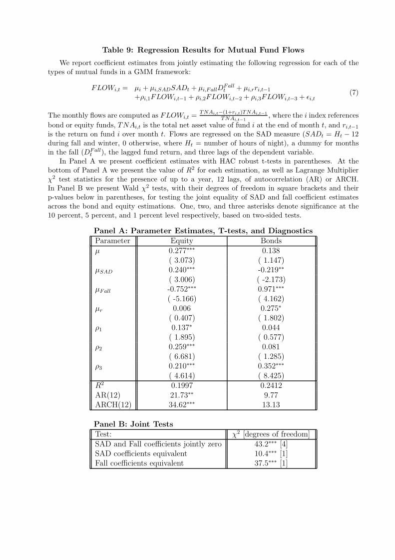
Table 9: Regression Results for Mutual Fund Flows
We report coefficient estimates from jointly estimating the following regression for each of thetypes of mutual funds in a GMM framework:
FLOWi,t = µi + µi,SADSADt + µi,FallDFallt + µi,rri,t−1
+ρi,1FLOWi,t−1 + ρi,2FLOWi,t−2 + ρi,3FLOWi,t−3 + εi,t(7)
The monthly flows are computed as FLOWi,t = TNAi,t−(1+ri,t)TNAi,t−1
TNAi,t−1, where the i index references
bond or equity funds, TNAi,t is the total net asset value of fund i at the end of month t, and ri,t−1
is the return on fund i over month t. Flows are regressed on the SAD measure (SADt = Ht − 12during fall and winter, 0 otherwise, where Ht = number of hours of night), a dummy for monthsin the fall (DFall
t ), the lagged fund return, and three lags of the dependent variable.In Panel A we present coefficient estimates with HAC robust t-tests in parentheses. At the
bottom of Panel A we present the value of R2 for each estimation, as well as Lagrange Multiplierχ2 test statistics for the presence of up to a year, 12 lags, of autocorrelation (AR) or ARCH.In Panel B we present Wald χ2 tests, with their degrees of freedom in square brackets and theirp-values below in parentheses, for testing the joint equality of SAD and fall coefficient estimatesacross the bond and equity estimations. One, two, and three asterisks denote significance at the10 percent, 5 percent, and 1 percent level respectively, based on two-sided tests.
Panel A: Parameter Estimates, T-tests, and DiagnosticsParameter Equity Bondsµ 0.277∗∗∗ 0.138
( 3.073) ( 1.147)µSAD 0.240∗∗∗ -0.219∗∗
( 3.006) ( -2.173)µFall -0.752∗∗∗ 0.971∗∗∗
( -5.166) ( 4.162)µr 0.006 0.275∗
( 0.407) ( 1.802)ρ1 0.137∗ 0.044
( 1.895) ( 0.577)ρ2 0.259∗∗∗ 0.081
( 6.681) ( 1.285)ρ3 0.210∗∗∗ 0.352∗∗∗
( 4.614) ( 8.425)R2 0.1997 0.2412AR(12) 21.73∗∗ 9.77ARCH(12) 34.62∗∗∗ 13.13
Panel B: Joint TestsTest: χ2 [degrees of freedom]SAD and Fall coefficients jointly zero 43.2∗∗∗ [4]SAD coefficients equivalent 10.4∗∗∗ [1]Fall coefficients equivalent 37.5∗∗∗ [1]
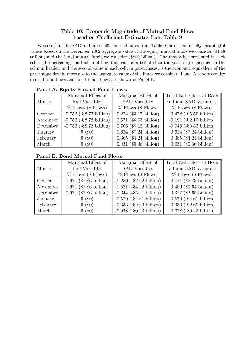
Table 10: Economic Magnitude of Mutual Fund Flowsbased on Coefficient Estimates from Table 9
We translate the SAD and fall coefficient estimates from Table 9 into economically meaningfulvalues based on the December 2002 aggregate value of the equity mutual funds we consider ($1.16trillion) and the bond mutual funds we consider ($809 billion). The first value presented in eachcell is the percentage mutual fund flow that can be attributed to the variable(s) specified in thecolumn header, and the second value in each cell, in parentheses, is the economic equivalent of thepercentage flow in reference to the aggregate value of the funds we consider. Panel A reports equitymutual fund flows and bond funds flows are shown in Panel B.
Panel A: Equity Mutual Fund Flows:Marginal Effect of Marginal Effect of Total Net Effect of Both
Month Fall Variable: SAD Variable: Fall and SAD Variables:% Flows ($ Flows) % Flows ($ Flows) % Flows ($ Flows)
October -0.752 (-$8.72 billion) 0.274 ($3.17 billion) -0.478 (-$5.55 billion)November -0.752 (-$8.72 billion) 0.571 ($6.63 billion) -0.181 (-$2.10 billion)December -0.752 (-$8.72 billion) 0.706 ($8.18 billion) -0.046 (-$0.53 billion)January 0 ($0) 0.624 ($7.24 billion) 0.624 ($7.24 billion)February 0 ($0) 0.365 ($4.24 billion) 0.365 ($4.24 billion)March 0 ($0) 0.031 ($0.36 billion) 0.031 ($0.36 billion)
Panel B: Bond Mutual Fund FlowsMarginal Effect of Marginal Effect of Total Net Effect of Both
Month Fall Variable: SAD Variable: Fall and SAD Variables:% Flows ($ Flows) % Flows ($ Flows) % Flows ($ Flows)
October 0.971 ($7.86 billion) -0.250 (-$2.02 billion) 0.721 ($5.83 billion)November 0.971 ($7.86 billion) -0.521 (-$4.22 billion) 0.450 ($3.64 billion)December 0.971 ($7.86 billion) -0.644 (-$5.21 billion) 0.327 ($2.65 billion)January 0 ($0) -0.570 (-$4.61 billion) -0.570 (-$4.61 billion)February 0 ($0) -0.333 (-$2.69 billion) -0.333 (-$2.69 billion)March 0 ($0) -0.028 (-$0.23 billion) -0.028 (-$0.23 billion)

Figure 1:
We plot average monthly bond returns, expressed on an annualized basis, based on the 1, 2, 5, 7,and 10 year bond indices. The averages are computed on the full range of CRSP data available:January 1941 through December 2001 for the 1, 2, and 5 year series; April 1941 through December2001 for the 5 and 7 year series; and May 1941 to December 2001 for the 10 year series.
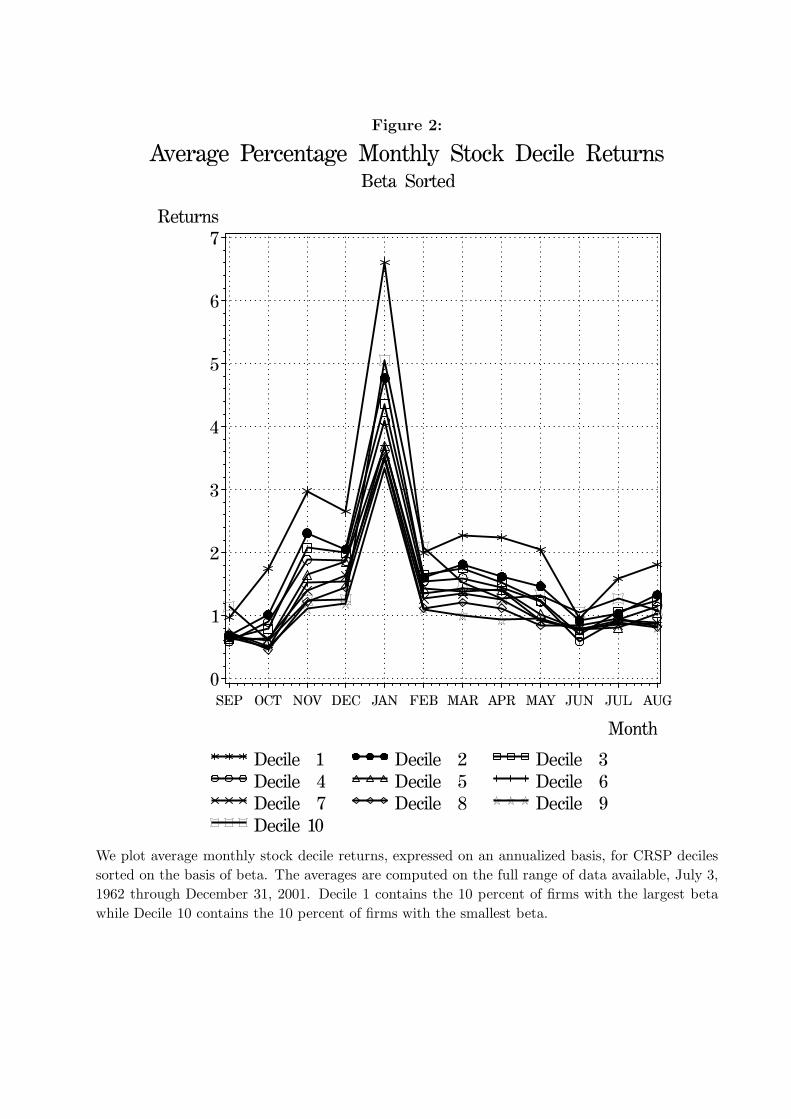
Figure 2:
We plot average monthly stock decile returns, expressed on an annualized basis, for CRSP decilessorted on the basis of beta. The averages are computed on the full range of data available, July 3,1962 through December 31, 2001. Decile 1 contains the 10 percent of firms with the largest betawhile Decile 10 contains the 10 percent of firms with the smallest beta.
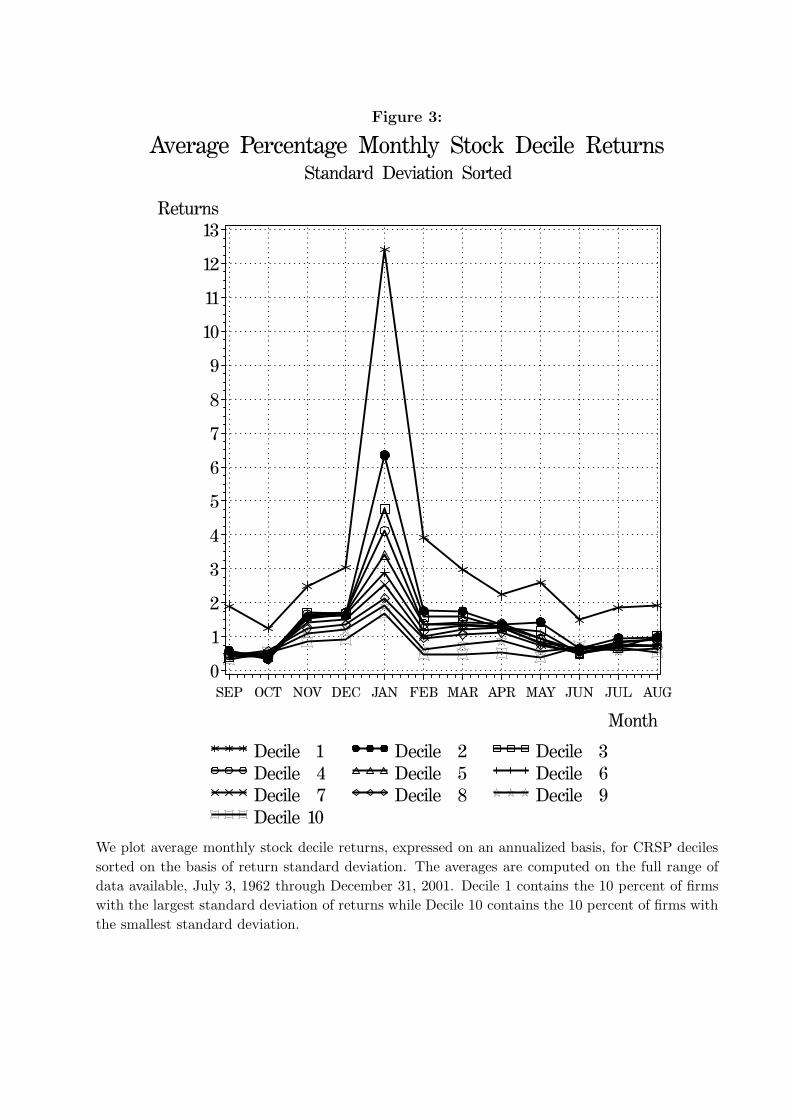
Figure 3:
We plot average monthly stock decile returns, expressed on an annualized basis, for CRSP decilessorted on the basis of return standard deviation. The averages are computed on the full range ofdata available, July 3, 1962 through December 31, 2001. Decile 1 contains the 10 percent of firmswith the largest standard deviation of returns while Decile 10 contains the 10 percent of firms withthe smallest standard deviation.
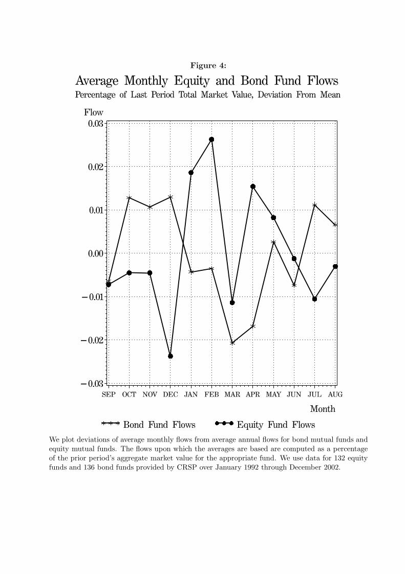
Figure 4:
We plot deviations of average monthly flows from average annual flows for bond mutual funds andequity mutual funds. The flows upon which the averages are based are computed as a percentageof the prior period’s aggregate market value for the appropriate fund. We use data for 132 equityfunds and 136 bond funds provided by CRSP over January 1992 through December 2002.
Top Related