


Languages
Pages
Legal


Remote Sensing of Snow using the
Chinese Fengyun satellites
Lingmei Jiang
State Key Laboratory of Remote Sensing Science, Jointly Sponsored by Beijing Normal University and the Institute of Remote Sensing and Digital
Earth, CAS, China School of Geography, Beijing Normal University, China

Snow monitoring with Chinese
Meteorological Fengyun satellites
1. A brief overview of Fengyun satellites
2. Snow depth estimation with FY-3/MWRI in China
3. Snow cover monitoring in China with multi-
sensor from Fengyun satellites data
4. Some examples of remote sensing of snow with
FY-3 (provided by Dr. Wu Shengli, NSMC)

FY –China’s weather satellites, including polar-
orbiting sun-synchronous orbits and
geosynchronuous orbit meteororolgical satellites
series.

Polar-Orbiting Geostationary
First Generation
Chinese Meteorological Satellites
FY-1A: 09/07/1988
FY-1B: 09/03/1990
FY-1C: 05/10/1999
FY-1D: 05/15/2002
Second Generation
FY-2A: 06/10/1997
FY-2B: 06/25/2000
FY-2C: 10/18/2004
FY-2D: 12/08/2006
FY-2E: 12/23/2008
FY-2F: 1/12/2012
First Generation
Second Generation
FY-3A: 05/27/2008
FY-3B: 11/05/2010
8 more: 2012-2020

Global Multi-orbit mosaic image

The 2nd generation polar-orbing satellites: FY3
series,including 11 sensors. Global, 3-D, all-weather,
Quantitative , muti-channel information of earth surface.

11 Sensors Onboard FY-3
(1) Visible and InfRared Radiometer (VIRR)
(2) MEdium ReSolution Imager (MERSI)
(3) InfRared Atmospheric Sounder (IRAS)
(4) MicroWave Temperature Sounder (MWTS)
(5) MicroWave Humidity Sounder (MWHS)
(6) MicroWave Radiation Imager (MWRI)
(7) Solar Backscatter Ultraviolet Sounder (SBUS)
(8) Total Ozone Mapping Unit (TOU)
(9) Earth Radiation Measurer (ERM)
(10) Solar Irradiation Monitor (SIM)
(11) Space Environment Monitor (SEM)

Instrument Channel Wavelength FOVs Resolution at Nadir
Purpose
VIRR 10 0.43 – 12.5μm 2048 1.1 km Cloud, aerosol, TPW,
vegetation, surface characteristics, surface T ,ice, snow etc.
MERSI 20 0.41 – 12.5 μm 2048/8192 1.1km/250m Ocean color, aerosol, TPW,
cloud, vegetation, surface characteristics, surface T ,ice, snow etc.
MWRI 12 10.65 – 150 GHz 240 15-70km
Rainrate, LWC, TPW, soil moisture, sea ice, SST, ice,
snow, etc.
IRAS 26 0.69 – 15.5 μm 56 17km T, q, total O3
MWTS 4 50 – 57 GHz 15 50-75km T
MWHS 5 150 – 183 GHz 98 15km q, surface characteristics
TOU 6 308 – 361 nm 31 50km Total O3
SBUS 12 250 – 340 nm 240 200km O3 profile
SIM 1 0.2~50μm Solar irradiance
ERM 4 0.2~3.8μm 0.2~50μm
150 2°×2° Earth's total radiation, Earth radiance
Instrument Parameters of FY-3

FY-3 Strategic Plan (2006-2020)
Global
All weather
3 Dimension
Quantitative
Multi-channels
2006FY-2D
2007FY-3A (TEST)
2010FY-2F
2008FY-2E
2009FY-3B (TEST)
2011FY-3AM1 2012FY-3PM1
2012FY-2G 2013FY-4A (TEST)
2013FY-3RM (TEST)
2015FY-4EAST1
2014FY-3AM2
2017FY-3AM3
2015FY-3PM2
2016FY-4WEST1
2017FY-4MS (TEST)
2018FY-3PM3
2016FY-3RM1 2019FY-3RM2
2019
FY-4EAST2
2020
FY-4WEST2
2020
FY-4MS
2008FY-3A
From Zhang Peng
2008FY-3A
2010FY-3B
2011FY-3AM1 2012FY-3PM1
2013FY-3RM
2014FY-3AM2
2015FY-3PM2
2017FY-3AM3
2016FY-3RM1
2018FY-3PM3
2019FY-3RM2
2013FY-4A
2015FY-4EAST1
2016FY-4WEST1
2017FY-4MS
2019FY-4EAST2 2020FY-4WEST2
2020FY-4MS

FY3A Global observation

Snow Importance
•High albedo – energy
balance
•Important water resource
• Frozen water represents
80% of all freshwater on
Earth.
• Snow melt runoff is the
major source of water to
rivers and groundwaters
over middle and high
latitude areas.
•Hazard (e.g. Extreme Snowfall
events in Southern China in 2008 &
2011)
Hydrological cycle overview
Why remote sensing of Snow

Snow: Remote Sensing/Satellite Capabilities
Snow Extent – Areal Coverage
optical (visible/infrared) – FY-2(VISSR)/FY-
3(VIRR,MERSI)
1km to 5 km spatial information
Snow Depth/Snow Water Equivalence
passive microwave – only proven satellite technique
for SWE retrieval
25 km grid, FY-3/MWRI

SMMR SSM/I AMSR-E FY-3B/MWRI AMSR2 1979-1987 1987-present 2002-2011.10 2010.11-present 2012.5.18-present
Passive Microwave Remote Sensing of Snow

What’s the difference between AMSR-E and FY-3/MWRI

Double difference between AMSR-E and MWRI
Yang et al.,(2011)

The brightness temperature difference between AMSR2 and FY3B/MWRI
36.5 GHz

• Approach for AMSR-E SWE product (Kelly et al.,2003) that
incorporates dynamic microwave response behaviour:
SD = FF(SDf) + (1-FF)(SDo)
(A*(18V-36V))
SD = FF * + (1-FF)* [ (A*(10V-36V)) + (B*(10V-18V)) ]cm
(1-FD*0.6)
Forest Non-forest
Medium snow
Non-forest
Deep snow
• Chang et al. (1996) and Foster et al. (1997) utilized the
following algorithms as:
Current approach
SWE = A + B ΔTb / (1-f) [mm]
• GlobSnow product: Data assimilation Bayesian approach
(Pulliainen,2006)
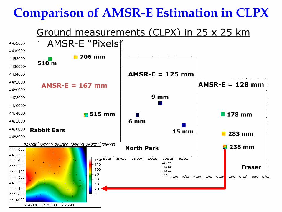
Fraser
283 mm
178 mm
238 mm
AMSR-E = 128 mm
North Park
9 mm
6 mm
15 mm
AMSR-E = 125 mm
Rabbit Ears
706 mm 510 mm
515 mm
AMSR-E = 167 mm
Ground measurements (CLPX) in 25 x 25 km AMSR-E “Pixels”
Comparison of AMSR-E Estimation in CLPX

Problems in SWE Estimation
1) Inhomogeneity: sub-pixel distribution
2)Vertical properties
3) Snow properties

Effects of Snow Grain Size on Brightness Temperature at Different Frequencies
• Depending on grain size, 37GHz has
saturation problem. But not lower
frequencies;
• Snow grain size has great impact on the
sensitivity of ΔTb(18GHz-37GHz) to snow
depth (or SWE);
• ΔTb(18GHz-37GHz) has multi-solutions.
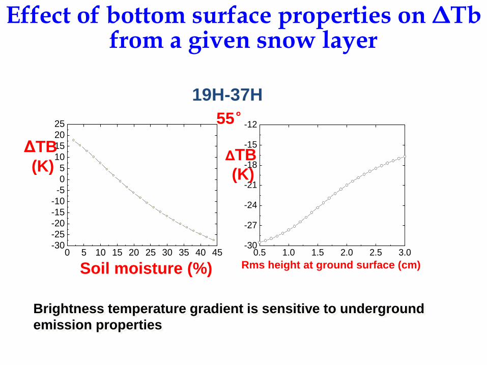
Effect of bottom surface properties on ΔTb from a given snow layer
0 5 10 15 20 25 30 35 40 45-30
-25-20
-15
-10-505
10
1520
25
0.5 1.0 1.5 2.0 2.5 3.0-30
-27
-24
-21
-18
-15
-12
19H-37H
55°
Soil moisture (%) Rms height at ground surface (cm)
ΔTB
(K) ΔTB
(K)
Brightness temperature gradient is sensitive to underground
emission properties

The effect of snow fraction on microwave emissivity

The effect of snow fraction on the brightness temperature difference based on the measured data
23
Snow-removed surface: mixed of compacted
snow/ice, grass, and soil (complex surface
condition)
http://nsidc.org/data/docs/daac/nsid
c0165_clpx_gbmr/index.html Snow fraction: (a)-(d): 75%-0%

Snow experiment- in the Northeast of China
-15
-10
-5
0
5
10
15
20
25
30
0 0.2 0.4 0.6 0.8 1
18v-36v
18h-36h
-15
-10
-5
0
5
10
15
20
25
30
0 0.2 0.4 0.6 0.8 1
18v-36v
18h-36h
Snow Fraction
ΔT
B
Snow Fraction
ΔT
B
Jilin, Changchun ,
2010
Snow-grass view field
Snow-ice mixed pixel
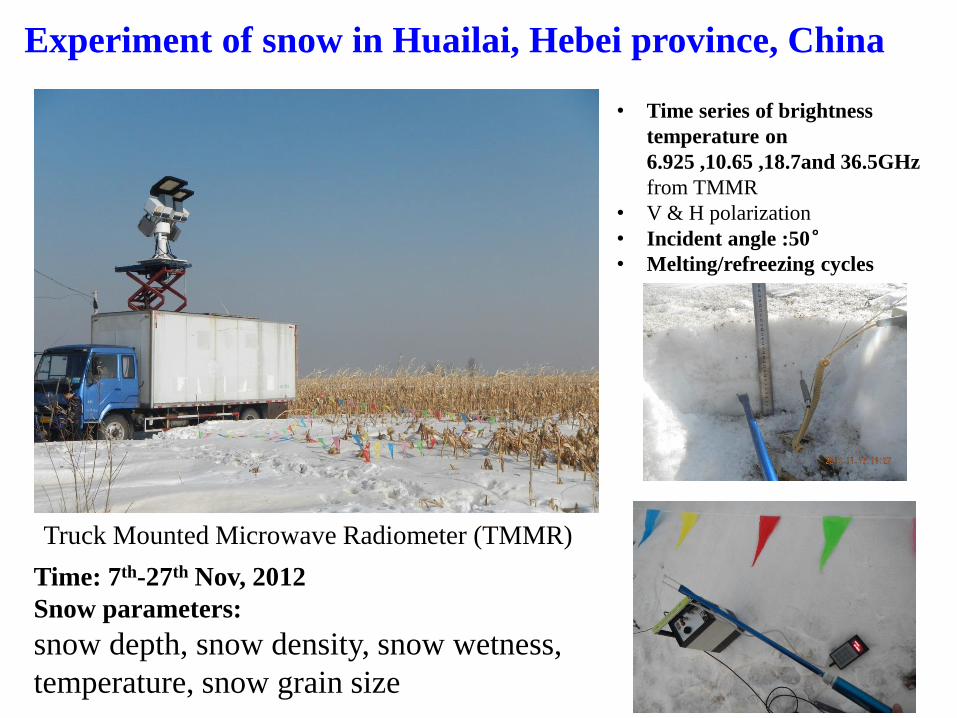
Experiment of snow in Huailai, Hebei province, China
Truck Mounted Microwave Radiometer (TMMR)
Time: 7th-27th Nov, 2012
Snow parameters:
snow depth, snow density, snow wetness,
temperature, snow grain size
• Time series of brightness
temperature on
6.925 ,10.65 ,18.7and 36.5GHz
from TMMR
• V & H polarization
• Incident angle :50°
• Melting/refreezing cycles

Experiment of snow in Baoding, Hebei province, China
• Time series of brightness
temperature on 6.925,
10.65, 18.7 and 36.5GHz
from TMMR
• V & H polarization
• Incident Angle: 0-
70°and 55°
• Machine Made snow
• Melting/refreezing cycles
Time: Feb. 26th – Mar. 3rd , 2011; Feb. 1st – Feb. 16th , 2012
Brightness temperature observations from TMMR
Snow depth measurement Snow grain size in microscope

Experiment of snow in Luancheng, Hebei province, China
2009/11/20 2009/11/14
2009/11/22 • Time: 13th-24th , Nov, 2009
• Time series of brightness
temperature on 10.65, 18.7
and 36.5GHz from TMMR
• V & H polarization
• Incident angle: 55° and 30-
60°
• Wet snow (due to melting)

Theoretical Radiative Transfer model
(DMRT-AIEM-MD model)
• Matrix Doubling method --- multi-scattering between
layer and boundaries
• AIEM (Advanced Integral Equation Model) ---
describing the underground emission signals and the
boundary conditions for the vector radiative transfer
model
• Snowpack properties --- the Mie scattering
assumption (DMRT)

Comparison of DMRT-AIEM-MD with experimental data(Weissfluhjoch, Switzerland , 1996) (1)
入射角
20° 70°
Wiesmann et al., (1996)
Frequency
Polarization
Table1. RMSE of the comparisons of the DMRT-AIEM-MD model
with the experiment data at Weissfluhjoch on Dec. 22, 1995
11 GHz 35 GHz 94 GHz Overall
v-pol 0.015 0.0009 0.015 0.013
h-pol 0.038 0.039 0.015 0.033
Polarization
Frequencies

Comparison of DMRT-AIEM-MD model with experimental data from LSOS at CLPX03 (2)
入射角
20° 70°
Feb. 22
Feb. 19 -25
55°
Hardy, et al., (2003)

Elevation :4120m
Mar. 24, 2008
冰沟地区的车载辐射计((RPG-8CH-DP)
观测
Comparison of DMRT-AIEM-MD model with experimental data from Bingou, Heihe basin (3)

Generated a simulating database with the theoretical emission model(DMRT-AIEM-MD)
The parameterized snow emission model
Paramete
rs
Mini
mum
Maxim
um step Units
Density 150 450 100 Kg m-3
Radius 0.2 1.6 0.2 mm
depth 0.1 2.0 0.1 m
Ground
rms
height
0.5 3.0 0.5 cm
Ground
rms slope 0.05 0.25 0.05 -
Soil
moisture 5 40 5 %
(1 )t v v v svs s
mp p p p p p p p
s
p p
E E Cf L E Cf E
Intercept slope E
The parameterized model Correction factor for multi-scattering
Here, Intercept and slope only depends on snow emission and attenuation

The parameterized emission model
2'v
pCf a b c d e
2 2exp ' ( ) ' ( )svs
pCf A B C D
' / cos( )r
where,a,b,c,d,e; and A, B,C,D are regression coefficients
Correction factor
V
H
DMRT-AIEM-MD model
10.7 GHz 18.7 GHz 36.5 GHz
RMSE: 0.0041 RMSE: 0.0071 RMSE: 0.010
RMSE: 0.0052 RMSE: 0.0087 RMSE: 0.013
Para
meterize
d
mo
del

Characterization of the Frequency Dependence of Underground Surface Emission Signals
The relationships of underground surface emissions with snow cover at
different frequencies simulated by AIEM model at 55°incidence angle
( ) ( , ) ( , ) ( )
( ) ( , ) ( , ) ( )
s s
p p
s s
p p
E X a X Ku b X Ku E Ku
E Ku a Ku Ka b Ku Ka E Ka
H V V/H
X-band
Ka-band
Ku-band
Ku-band
At given snow density, With different snow density, refractive angle varying, at the same incidence angle

Proposed Technique for Removing Underground Surface Emission Signal
)2(
)2()2(*
)1(
)1()1(
fslope
fInterceptfEba
fslope
fInterceptfE t
p
t
p
)(
)()()(
fslope
fInterceptfEfE
t
ps
p
At each frequency
At a given polarization and two frequencies,
( 1) * ( 2)t t
p pE f A B E f
Here, A, B are only related to snow properties.
( 1) ( 2)s s
p pE f a b E f
Assuming known temperatures

Inversion algorithm tested with simulated data from theoretical model
2exp( log( log( )))swe a b A c A d B
1 1
2 2
( ) ( )
( ) ( )
t t
v h
t t
v h
E f E fB
E f E f
Input SWE (m)
RMSE=0.034
Using A and B, we could estimate
SWE by this following regression
equation,
( 1) ( 1)t t
p pA E f B E f
SWE
A B
Here, a, b, c, d are regression coefficients.
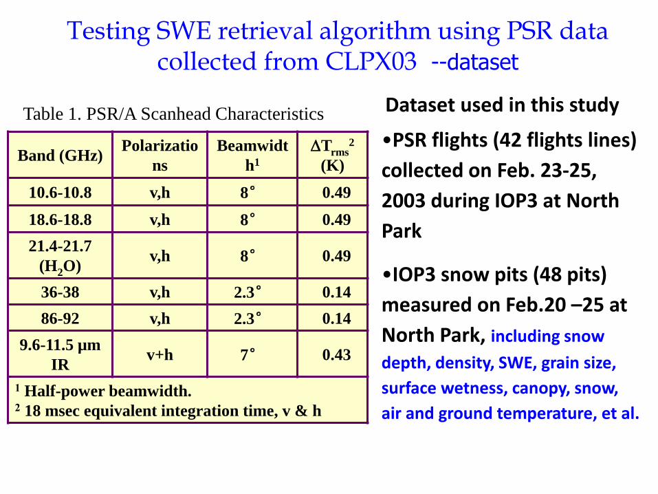
Testing SWE retrieval algorithm using PSR data collected from CLPX03 --dataset
•PSR flights (42 flights lines)
collected on Feb. 23-25,
2003 during IOP3 at North
Park
•IOP3 snow pits (48 pits)
measured on Feb.20 –25 at
North Park, including snow
depth, density, SWE, grain size,
surface wetness, canopy, snow,
air and ground temperature, et al.
Table 1. PSR/A Scanhead Characteristics
Band (GHz) Polarizatio
ns
Beamwidt
h1
Trms2
(K)
10.6-10.8 v,h 8° 0.49
18.6-18.8 v,h 8° 0.49
21.4-21.7
(H2O) v,h 8° 0.49
36-38 v,h 2.3° 0.14
86-92 v,h 2.3° 0.14
9.6-11.5 µm
IR v+h 7° 0.43
1 Half-power beamwidth. 2 18 msec equivalent integration time, v & h
Dataset used in this study

Testing SWE retrieval algorithm using PSR data collected from CLPX2003 --- Comparison
Measured SWE (mm)
New technique
AMSR-E algorithm
1. From the comparison, AMSR-E inversion algorithm overestimated ground measurements of SWE
2. The new technique developed also overestimated SWE, but it showed some improvement on AMSR-E retrieval
3. Assume fully snow covered pixel for PSR in this validation. The effect of mixed-pixel, vegetation and topography on the retrieval algorithm has to be considered in the inversion technique development.
Esti
mat
ed

We evaluated the snow emission theoretical model (DMRT-
AIEM-MD) with three experimental dataset. The comparisons
indicated our model could predict snow emission reasonable
well.
We developed a simple and high accuracy parameterized
emission model based on simulated snow emission database.
A physically based inversion technique is developed in this
study using the snow emission model. Through testing with
PSR data, this new inversion algorithm showed better results
than AMSR-E did, but still needs to be improved for the actual
application.
We could estimate snow properties by cancelling out
underground surface emission signal using their relationship at
different frequencies.
Summary

Validation of AMSR-E SWE in China
RMSE=26.5mm

Comparison between MOD12Q1 and Land use map
LULC (2000)
MOD12Q1数据(2004)
MOD12Q1(2004)
The LULC map (provided by the Data Center for Resources and
Environmental Sciences ) show that grasslands of the Qinghai-Tibet and
Yunnan-Guizhou plateaus are substantially more consistent with
vegetation maps.
Northeast China has the important natural forest areas, especially in the
Daxinganling, Xiaoxinganling, and Changbaishan mountains.

Land cover
Snow depth inversion algorithms Regression (R^2)
Regression RMSE (cm)
Regression samples
Validation samples
Validation RMSE (cm)
Farmland
Sd=-4.235+0.432×d18v36h+1.074× d89v89h
0.417 4.47 2888 448 4.51
Grass Sd=4.320+0.506×d18h36h-0.131×d18v18h +0.183×d10v89h-0.123×d18v89h
0.575 3.57 2894 487 2.84
Bare ground
Sd=3.143+0.532×d36h89h-1.424×d10v89v+1.345×d18v89v-0.238d36v89v
0.589 2.15 177 40 1.98
forest Sd=11.128-0.474×d18h36v-1.441 ×d18v18h+0.678 ×d10v89h-0.649×d36v89h
0.135 5.61 1163 188 6.28
farmlandfarmlandforestforestbarenbarengrassgrass SDfSDfSDfSDfSD
Snow depth retrieval algorithm over
China A linear decomposition technique of mixed pixels was incoporated.

Validation of FY-3/MWRI snow depth (SWE) algorithm
RMSE=5.58cm
Compared with AMSR-E SWE product
Compared with ground station measurements
AMSR-E overestimated in China

Comparison of AMSR-E SWE and FY3B/MWRI SWE in spatial distribution
AMSR-E FY3B/MWRI Jan 14, 2011

Time series snow depth RMSE of AMSR-E and FY-3B/MWRI with ground observation in China
(black line: AMSR-E RMSE; blue line: FY3B-MWRI RMSE; red line: stations averaged snow depth)
Dec. 1, 2010 to Feb. 28, 2011

Retrieval errors spatial distribution
between AMSR-E and FY-3/MWRI
AMSR-E
FY-3/MWRI

Summary (snow depth retrieval)
• The MWRI aboard the FY-3 platform, the first microwave
radiometer on meteorological satellites show the capability to
estimate snow depth in China.
• Through validation with ground observations, FY-3 snow depth
retrieval algorithms performed well for grassland and farmland
surfaces, but underestimated snow depth for forested areas.
• FY-3/MWRI performs better than AMSR-E SWE product in
China, especially over forest-covered area with complex terrain,
such as in Northeast China and North Xinjiang.
• Forest, complex terrain issues are still ongoing in the operational
algorithm.

Snowfall events in
Southern China 2008-1-10~2-10 2011-1-18~1-22; 2011-2-25~3-3
500m spatial resolution
Sub-pixel technique
Shi(2012)
MODIS fractional snow
cover
25km spatial resolution
AMSR-E L3 Products
from NASA
AMSR-E SWE
5km spatial resolution
Northern hemisphere
multi-sensor snow cover
product from NOAA
IMS snow cover
Interactive Multi-sensor Snow
and Ice Mapping System
Input data in IMS: - Polar & Geostationary satellite optical data
- Microwave snow products
- Meteorological observations

• Monitoring Snow cover using Polar-orbit satellites
– NOAA-AVHRR, Aqua&Terra-MODIS, FY3-MERSI…
– Optical-infrared
• High spatial & spectral resolution
• Seriously affected by cloud
– Passive microwave
• Suitable for dry snow in current algorithms
• Coarse resolution, SWE products present over-estimation in
China
• Geostationary satellites
– High temporal resolution
– GOES, MSG, MTSAT-2, FY-2…
– Lower spatial resolution
– Providing in real-time snow information
Remote sensing of snow with multi-sensors
data
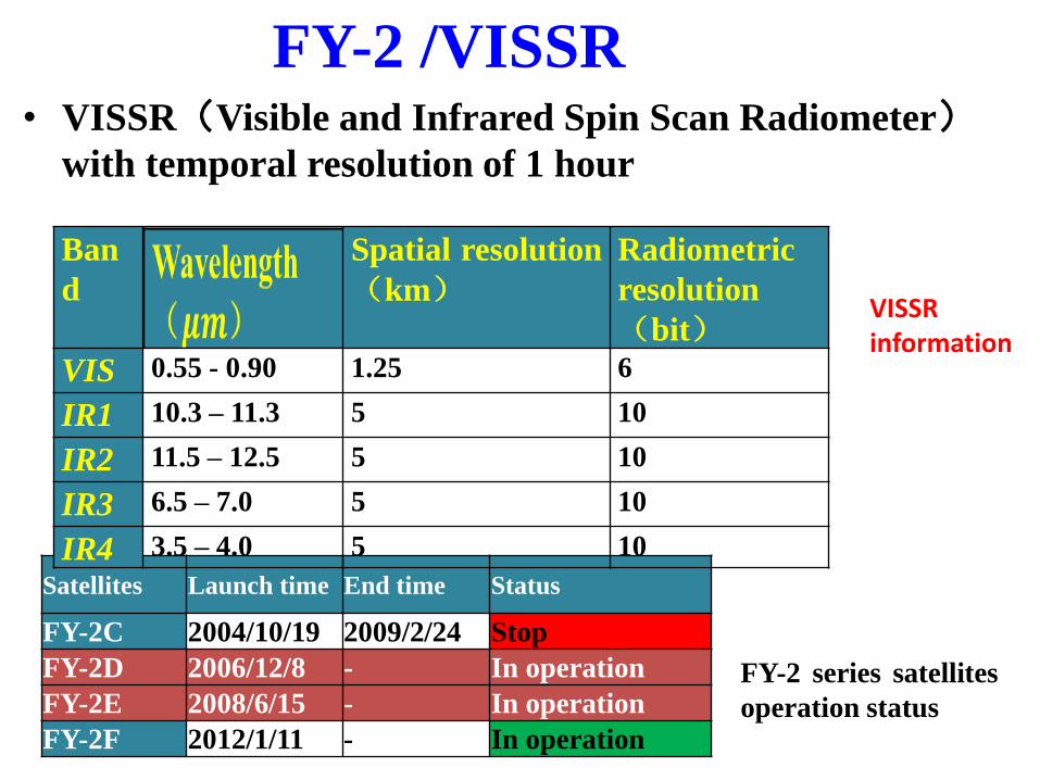
FY-2 /VISSR • VISSR(Visible and Infrared Spin Scan Radiometer)
with temporal resolution of 1 hour
Satellites Launch time End time Status
FY-2C 2004/10/19 2009/2/24 Stop
FY-2D 2006/12/8 - In operation
FY-2E 2008/6/15 - In operation
FY-2F 2012/1/11 - In operation
FY-2 series satellites
operation status
Ban
d
Spatial resolution
(km)
Radiometric
resolution
(bit)
VIS 0.55 - 0.90 1.25 6
IR1 10.3 – 11.3 5 10
IR2 11.5 – 12.5 5 10
IR3 6.5 – 7.0 5 10
IR4 3.5 – 4.0 5 10
VISSR information

Data pre-process
• FY-2D and FY-2E VISSR data are used
– FY-2D located in 86.5°E;FY-2E located in 104.5°E
– Combination of FY-2D and FY-2E: temporal resolution can be
improved to half an hour
• VISSR data resampled to 0.05 degree latitude-longitude
projection
• Angular correction: Raw data/ cos (Solar zenith angle)
FY-2E (After resampled) Jan. 12, 2011 FY-2E visible raw data

Snow cover algorithm • Algorithm for every one hour VISSR data
– Threshold-based decision tree spectral classification
• High reflectance of 0.6 m and low reflectance of 3.9 m
• Brightness temperature difference of IR2 and IR4; IR4 and IR1
• Thresholds setting based on scatterplots and histograms of snow-
covered, snow-free and cloud samples
– Training data were selected based on station observations of year 2010.

Snow cover algorithm
Threshold Classification Rule
number
Snow-free 1
Snow-free 2
Snow-free 3
Snow-free 4
Snow-covered 5
Snow-covered 6
Cloud 7
Cloud 8
Cloud 9
Cloud 10
Cloud 11
Cloud 12
Phase 1 Phase 2

Multi-temporal data in snow cover
mapping • Each temporal snow cover map of FY-2D and FY-2E/ VISSR
– Every one hour VISSR data using snow cover algorithm
– Solar zenith angle should lower than 80 degree
• Combination of multi-temporal snow cover maps daily
– Rules: Snow-covered > Snow-free > Cloud
– Purpose: Obtain the snow cover map with less cloud obscuration
Multi-temporal snow cover maps composited snow cover map
Jan 10,2011

Cloud removing - Spatial filtering – Object:cloud pixels
– Method:Based on the 8 neighboring pixels
– If the 8 pixels are all snow-free, then the cloud pixel reclassified to
snow-free; If the 8 pixels are all snow-covered, then the cloud
pixel reclassified to snow-covered
Spatial and temporal
filtering techniques are
widely used in MODIS
snow cover maps, which
show good performance
in reducing cloud
obscuration
Snow-free pixel
Snow-covered pixel
Cloud pixel

Cloud removing – Temporal filtering – Object:Cloud pixels
– Method:Examine the previous and the next day classification of
the cloud pixel
– If both the previous and the next day are snow-free, the cloud pixel
is reclassified to snow-free; If both the previous and the next day
are snow-covered, the cloud pixel is reclassified to snow-covered
Current Previous day Next day
Processed after
temporal filtering
Snow-free
Snow-covered
Cloud

Cloud removing- Combined with FY-
3B/ MWRI • Cloud still can’t be removed after spatial-temporal filtering
• Combination with passive microwave snow cover can remove the
cloud completely
• FY-3B was launched in November, 2010
• MWRI: Microwave Radiation Imager
• Snow cover algorithm---Grody(1996)
Center Frequencies
(GHz)
Bandwidth (MHz)
Sensitivity (K)
IFOV (km)
10.65 180 0.6 51*85
18.7 200 1.0 30*50
23.8 400 1.0 27*45
36.5 900 1.0 18*30
89.0 2*2300 2.0 9*15

Accuracy assessment
• 699 meteorological stations observations
• Stations observations as true value
• Time:Two winter seasons(Dec. 2010 to Feb. 2011 & Dec. 2011 to
Feb. 2012)
Satellite:
snow-covered
Satellite:
snow-free
Station snow-
covered
a b
Station snow-
free
c d
OA:Overall accuracy of snow cover images
IU:Under-estimation of snow cover images
IO:Over-estimation of snow cover images

Snow cover products for comparison
• NOAA IMS snow cover product
– 4 km spatial resolution,Northern hemisphere
– Widely used for comparison and validation
– Multi-sensor data and products combination
• MODIS snow cover product
– Most widely used snow cover product
– MOD10A1 & MYD10A1 are used
– 500 m spatial resolution
MOD10A1, MYD10A1 and IMS snow cover
products are resampled to 0.05 degree for
comparison with FY2D/E snow cover images

Comparison of FY-2DE and MODIS snow cover
Snow cover map of FY-2DE Snow cover map of MOD10A1+MYD10A1
Cloud coverage
percentage (two
winter seasons):
MODIS_DC:46.75
%
FY_2DE:18.63%

Comparison Fengyun snow maps
with IMS product FY-2DE processed spatial-temporal filtering
FY-3B\MWRI
FY-2DE & FY-3B
IMS
Jan. 10,2011

Overall accuracy under clear-sky
condition
FY_2DE_ST:FY-2DE processed spatial-temporal filtering
FY-3B/MWRI:FY-3B MWRI
FY_2DE_FM:Combination of FY_2DE_ST & FY-3B/MWRI
IMS:NOAA IMS
91.90%
86.18%
91.37%
92.51%
OA:

DEM(m)
Accuracy assessment with DEM
IMS IMS
IMS
FY_2DE_FM FY_2DE_FM
FY_2DE_FM
Overestimated error
Underestimated error
Overall accuracy

Summary (snow cover)
• High temporal resolution of geostationary satellite data
show potential to obtain more information of snow surface.
• Combination of FY-2D/E and FY-3B has showed high
accuracy snow cover products and with less cloud
obscuration, but overestimated in some mountain regions
(e.g. TP). NOAA IMS snow cover product showed much
overestimation is such areas.
• This is still need to be improved, by improving spatial
resolution, fraction snow cover,….

4. Some examples of remote sensing of snow cover with FY-3

Snow cover product of FY-3 and MODIS MODIS/TERRA 20050211
B-6-2-1
VIRR 日雪盖
MOD10C daily snow fraction
水体 0.0 0.1 0.2 0.3 0.4 0.5 0.6 0.7 0.8 0.9 1.0 水体 0.0 0.1 0.2 0.3 0.4 0.5 0.6 0.7 0.8 0.9 1.0
MOD10C daily cloud fraction
FY-3/VIRR

Demonstration products (optical)
FY3A/VIRR

Demonstration products (microwave)

Snow depth monitoring and analysis system
Global swath Brightness temperature map

China swath Brightness temperature map

China daily snow depth map

5-day composite
snow depth map
by FY-3

Thank you for your attention!
Top Related